1

2

3

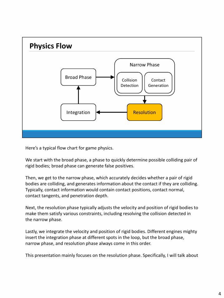
Here’s a typical flow chart for game physics.

We start with the broad phase, a phase to quickly determine possible colliding pair of rigid bodies; broad phase can generate false positives.

Then, we get to the narrow phase, which accurately decides whether a pair of rigid bodies are colliding, and generates information about the contact if they are colliding. Typically, contact information would contain contact positions, contact normal, contact tangents, and penetration depth.

Next, the resolution phase typically adjusts the velocity and position of rigid bodies to make them satisfy various constraints, including resolving the collision detected in the narrow phase.

Lastly, we integrate the velocity and position of rigid bodies. Different engines mighty insert the integration phase at different spots in the loop, but the broad phase, narrow phase, and resolution phase always come in this order.

This presentation mainly focuses on the resolution phase. Specifically, I will talk about

4

a popular way to implement the resolution phase called sequential impulse. This approach is popularized by Erin Catto, author of the famous Box2D physics engine.

4

5

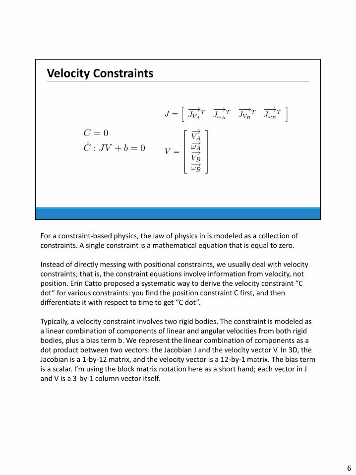
For a constraint-based physics, the law of physics in is modeled as a collection of constraints. A single constraint is a mathematical equation that is equal to zero.

Instead of directly messing with positional constraints, we usually deal with velocity constraints; that is, the constraint equations involve information from velocity, not position. Erin Catto proposed a systematic way to derive the velocity constraint “C dot” for various constraints: you find the position constraint C first, and then differentiate it with respect to time to get “C dot”.

Typically, a velocity constraint involves two rigid bodies. The constraint is modeled as a linear combination of components of linear and angular velocities from both rigid bodies, plus a bias term b. We represent the linear combination of components as a dot product between two vectors: the Jacobian J and the velocity vector V. In 3D, the Jacobian is a 1-by-12 matrix, and the velocity vector is a 12-by-1 matrix. The bias term is a scalar. I’m using the block matrix notation here as a short hand; each vector in J and V is a 3-by-1 column vector itself.

6

Sometimes, we will have an inequality constraint instead of an equality constraint. For instance, “C dot greater than or equal to zero”. Implementation-wise, this is very simple to solve: we just impose the equality constraint “C dot equal to zero” whenever “C dot is greater than or equal to zero”.

7

For a violated velocity constraint, we would like to apply a change to the velocity vector (delta V) to make the constraint satisfied again.

Here, I’m going to ask you to take a leap of faith with me and believe that “delta V” is proportional to “M inverse J t (transpose)”, where M is the mass matrix.

The proportional constant is lambda, also known as the Lagrangian multiplier. If we can find the lambda for a violated constraint, we can apply a fix to the velocity vector and satisfy the constraint again.

8

To find lambda, we need to do some algebra.

V is the original velocity vector, and delta V is the change to the velocity vector; so, V plus delta V is our final velocity vector. The final velocity vector should satisfy the constraint when plugged into the original constraint equation. We substitute “delta V” with “M inverse J t lambda”, and then we can find the symbolic solution for lambda. Lambda is essentially the impulse required to fix a constraint, and its also known as the Lagrangian multiplier.

We sometimes refer to “J M inverse J t” as the “effective mass”.

9

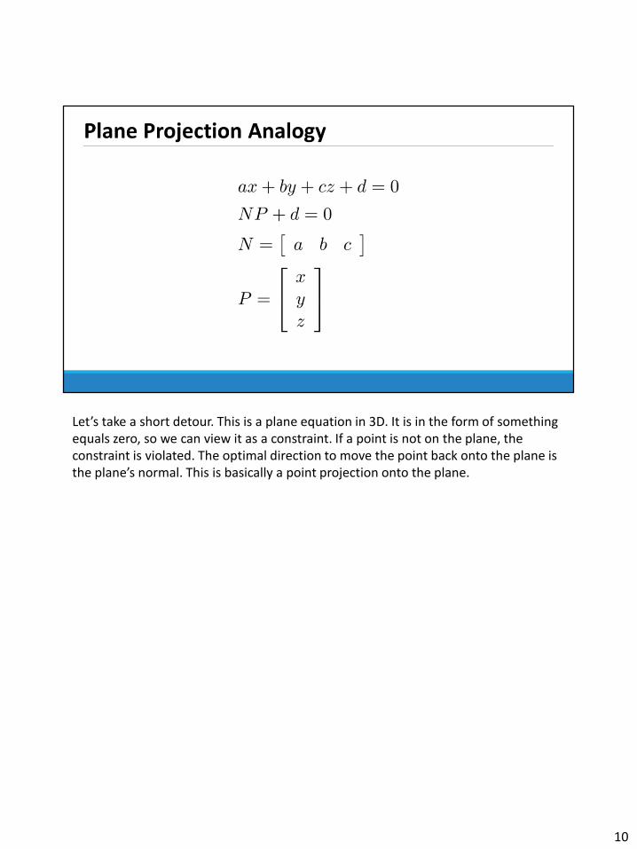
Let’s take a short detour. This is a plane equation in 3D. It is in the form of something equals zero, so we can view it as a constraint. If a point is not on the plane, the constraint is violated. The optimal direction to move the point back onto the plane is the plane’s normal. This is basically a point projection onto the plane.

10

On the left, we see the plane equation, and the change to the point to fix the constraint is proportional to the plane normal. Looks familiar? Here’s its counterpart in velocity constraints. The velocity constraint is basically a 12D plane, and the plane normal is the Jacobian. There is one caveat. We need to take the rigid body’s mass and inertia tensor into account, so we modify the direction of correction by “M inverse”. This is why “delta V” is proportional to “M inverse J t”.

11

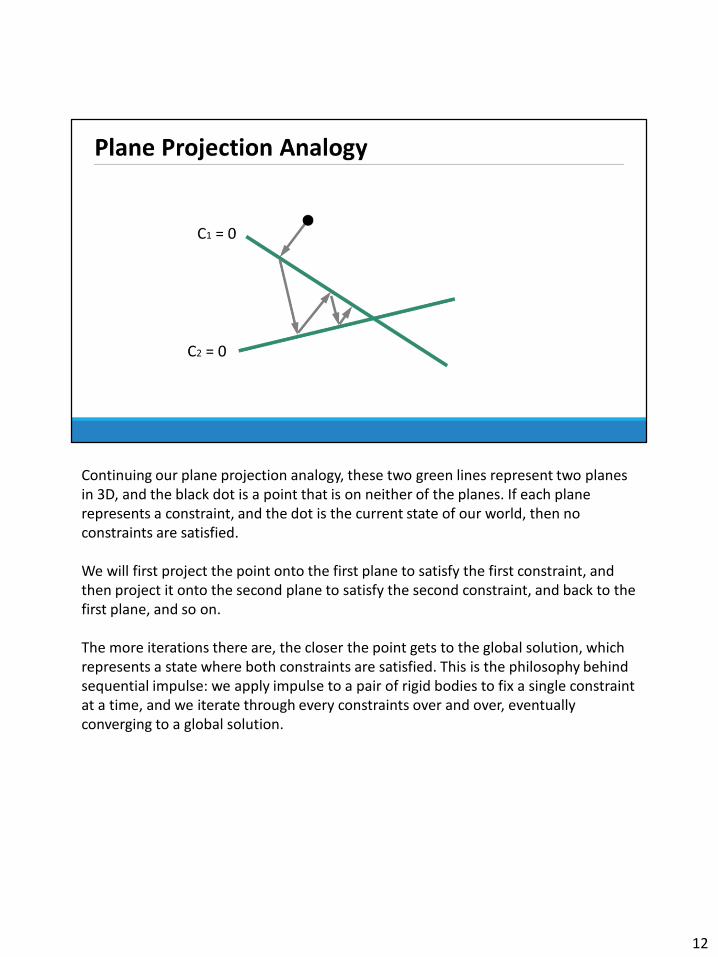
Continuing our plane projection analogy, these two green lines represent two planes in 3D, and the black dot is a point that is on neither of the planes. If each plane represents a constraint, and the dot is the current state of our world, then no constraints are satisfied.

We will first project the point onto the first plane to satisfy the first constraint, and then project it onto the second plane to satisfy the second constraint, and back to the first plane, and so on.

The more iterations there are, the closer the point gets to the global solution, which represents a state where both constraints are satisfied. This is the philosophy behind sequential impulse: we apply impulse to a pair of rigid bodies to fix a single constraint at a time, and we iterate through every constraints over and over, eventually converging to a global solution.

12

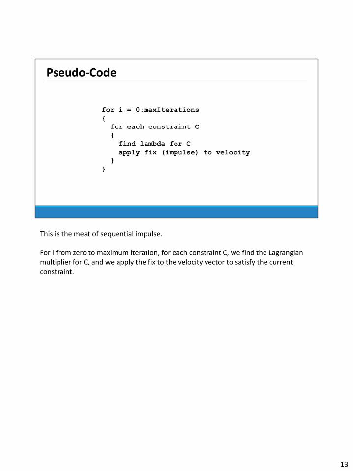
This is the meat of sequential impulse.

For i from zero to maximum iteration, for each constraint C, we find the Lagrangian multiplier for C, and we apply the fix to the velocity vector to satisfy the current constraint.

13

14

Let’s look at a concrete example on how we would derive a velocity constraint. C is a contact constraint, which states that the contact points should be separated along the contact normal. We then expand P into a combination of center of mass and offset vector. Next, we differentiate C to get C dot. By shifting terms around, we can obtain our Jacobian for contact constraints. This Jacobian has a geometric interpretation: the projection of relative velocity between the contact points onto the contact normal should always be zero or separating. By changing the velocity vector to satisfy a contact constraint, the two rigid bodies will have zero relative velocity along the contact normal at the contact points. Note that we don’t have restitution right now.

15

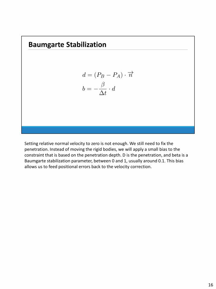
Setting relative normal velocity to zero is not enough. We still need to fix the penetration. Instead of moving the rigid bodies, we will apply a small bias to the constraint that is based on the penetration depth. D is the penetration, and beta is a Baumgarte stabilization parameter, between 0 and 1, usually around 0.1. This bias allows us to feed positional errors back to the velocity correction.

16

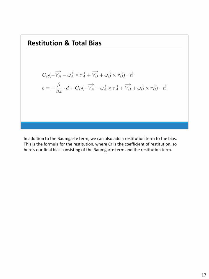
In addition to the Baumgarte term, we can also add a restitution term to the bias. This is the formula for the restitution, where Cr is the coefficient of restitution, so here’s our final bias consisting of the Baumgarte term and the restitution term.

17

Frictions are actually very easy to deal with. Remember that the Jacobian in the contact normal direction has a geometric meaning? It zeroes out the component of relative velocity in the contact normal direction. We can swap out the normal vector with tangent vectors in the Jacobian, and we get two Jacobians that zero out the tangent component of relative velocity.

18

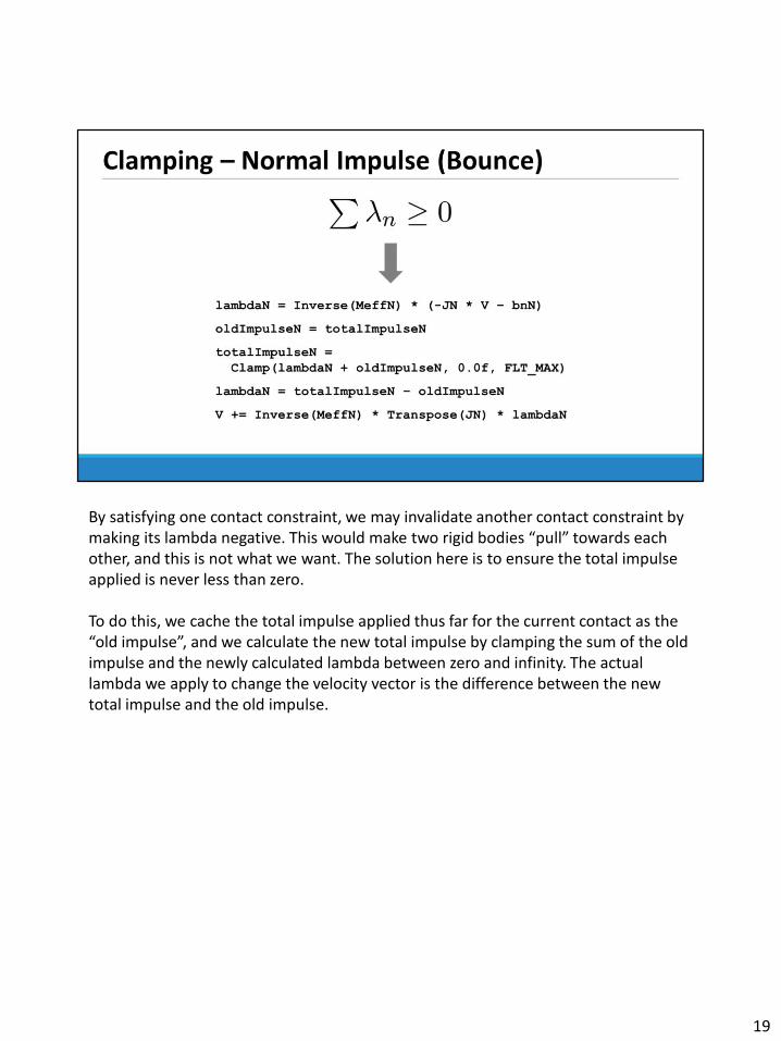
By satisfying one contact constraint, we may invalidate another contact constraint by making its lambda negative. This would make two rigid bodies “pull” towards each other, and this is not what we want. The solution here is to ensure the total impulse applied is never less than zero.

To do this, we cache the total impulse applied thus far for the current contact as the “old impulse”, and we calculate the new total impulse by clamping the sum of the old impulse and the newly calculated lambda between zero and infinity. The actual lambda we apply to change the velocity vector is the difference between the new total impulse and the old impulse.

19

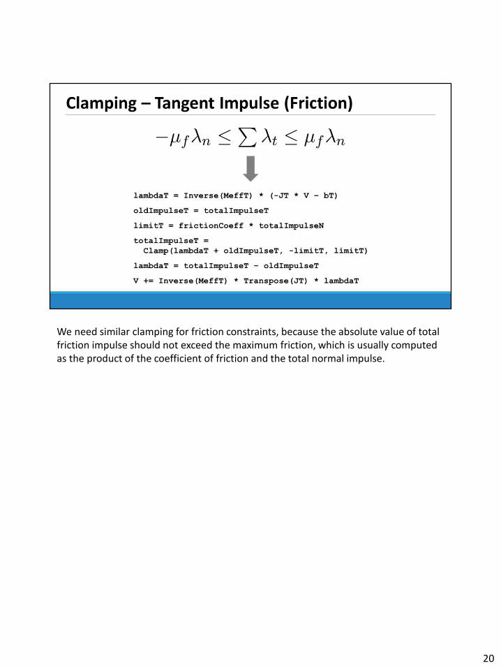
We need similar clamping for friction constraints, because the absolute value of total friction impulse should not exceed the maximum friction, which is usually computed as the product of the coefficient of friction and the total normal impulse.

20

21

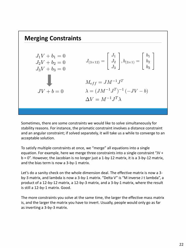
Sometimes, there are some constraints we would like to solve simultaneously for stability reasons. For instance, the prismatic constraint involves a distance constraint and an angular constraint; if solved separately, it will take us a while to converge to an acceptable solution.

To satisfy multiple constraints at once, we “merge” all equations into a single equation. For example, here we merge three constraints into a single constraint “JV + b = 0”. However, the Jacobian is no longer just a 1-by-12 matrix, it is a 3-by-12 matrix, and the bias term is now a 3-by-1 matrix.

Let’s do a sanity check on the whole dimension deal. The effective matrix is now a 3-by-3 matrix, and lambda is now a 3-by-1 matrix. “Delta V” is “M inverse J t lambda”, a product of a 12-by-12 matrix, a 12-by-3 matrix, and a 3-by-1 matrix, where the result is still a 12-by-1 matrix. Good.

The more constraints you solve at the same time, the larger the effective mass matrix is, and the larger the matrix you have to invert. Usually, people would only go as far as inverting a 3-by-3 matrix.

22

23

Before diving into implementing a full-blown physics engine with fancy constraints, I encourage you to do a simple homework first: mouse constraints. It is a very easy constraint to implement, and you don’t need any broad phase or narrow phase, just the resolution phase and integration phase.

The constraint is simple: we want the position difference between an anchor point on a rigid body and the mouse position to be zero.

We differentiate this equation with respect to time, and we get “C dot”. We let the mouse position be considered as a constant, so its derivative is zero. With “C dot”, we can easily write out the Jacobian. It forces the anchor point on the constrained rigid body to have zero relative velocity in world space.

The bias term uses Baumgarte stabilization to correct positional errors.

The effective mass matrix is still using the same formula “J M inverse J t”. Note that this is a multi-constraint with 3 constraints, so the effective mass matrix is a 3-by-3 matrix. During calculation, the “mass of the mouse cursor” should be treated as infinity, since it will not be moved by the constraint at all.

24

NOTE: The DigiPen Distance website is only available to DigiPen personnels only.

25

26