constraint-based motion adaptation paper presents constraint-based motion adaptation, ... we provide...

∗ †

∗

†

Abstract

Keywords:

Constraint-based Motion Adaptation

[email protected]

The Journal of Visualization and Computer Animation

Michael Gleicher Peter LitwinowiczApple Research Laboratories

Apple Computer, Inc.Cupertino, CA 95014, USA

November 2, 1998

current address: Vision Technology Center, Autodesk, Inc., 2465 Latham St. Suite 101,Mountain View, CA 94040,

current address: 1059 Noe St., San Francisco, CA 94114

To appear in .Edited draft from June, 1996Edited draft from May, 1997Edited draft from August 12, 1997Edited draft from September 1, 1997This version October 16, 1997, processed November 2, 1998

1

Today’s computer animators have access to many systems and tech-niques to author high quality motion. Unfortunately, available techniquestypically produce a particular motion for a specific character. In this paper,we present a constraint-based approach to adapt previously created motionsto new situations and characters. We combine constraint methods that com-pute changes to motion to meet specified needs with motion-signal process-ing methods that modify signals yet preserve desired properties of the origi-nal motion. The combination allows the adaptation of motions to meet newgoals while retaining much of the motion’s original quality.

computer animation, motion adaptation, constraint solving, mo-tion displacement and warping.

1 Introduction

Creating high quality motion for animation is a tedious and difficult task. Evenwith advanced computer animation tools, creating motion that is purposeful, ex-pressive and attractive requires considerable effort, typically requiring skilled an-imators or actors and engineers using motion capture equipment. The cost, diffi-culty, and talent required puts motion generation out of the reach of many potentialusers.

Despite its high cost, generated motion is not commonly reusable. More oftenthan not, motion will only be valuable for a particular model and is almost cer-tainly unusable for more than a particular scenario. For instance, the motion ofa woman reaching for a doorknob will be precisely that — the motion will mostprobably be useless for having the character pick up something from the ground,or for a different character, or even for a different doorknob.

Computer animation research has evolved 4 general strategies to the problemof producing motion. The first is to improve the tools used for keyframing; for ex-ample, by adding inverse kinematics to control models. While such methods canmake it much less tedious to produce motion, they are predominantly a tool forhelping skilled animators produce single-use motions. Another strategy uses algo-rithmic or simulation methods to generate motions based on descriptions of goals.While such methods have the promise of generating motions for non-experts byallowing them to simply specify their needs, they are, at present, of limited use.A third approach tracks motion of real world actors or objects. This approach re-quires having real motion to capture and typically requires sophisticated sensorsand processing.

A fourth, more recent, approach to the motion problem attempts to adapt exist-ing motion generated by one of the other methods. Such adaptive methods couldput animation capabilities in the hands of inexperienced animators, allowing theuse of motion created by others in new scenarios and with other characters. It canalso enable “on-the-fly” adaptation of motions, creating motion as needed in aninteractive context.

One promising approach to motion adaptation, presented by Bruderlin andWilliams[8], treats motions as signals and applies some traditional signal process-ing methods to adapt them, while preserving aspects of their character. A variantof one of their most interesting methods, motion-displacement mapping, was si-multaneously introduced as “motion warping” by Witkin and Popovic [46]. Un-fortunately, as initially presented the methods fall short of being able to realizeour goals. In this paper, we present an approach to motion adaptation that extends

2

2 Previous Approaches

the originally published methods to better address their shortcomings.This paper presents constraint-based motion adaptation, an approach that uses

numerical constraint solving techniques to alter motions so that they meet desiredgoals while preserving as much of the original motion as possible. We combineelements of two prior approaches: motion signal processing alters motion in waysthat preserve desired qualities; and constraint-based direct manipulation (a gen-eralization of inverse kinematics) provides a flexible mechanism for specifyinggoals. Together, these provide an approach whereby a user can create new mo-tions that have the character of the original, but meet a set of new requirements.

The basic idea of our approach is to treat motion adaptation as a constrainedoptimization problem: what is the smallest change that can be made to a motionsignal in order to meet a set of specified goals? Like the spacetime constraintmethods of Witkin and Kass [45] and Cohen [9], we solve a constraint problem forthe entire motion. In constrast, most other constraint methods that process eachframe individually. The reward for solving these large numerical problems is amethod that affords flexibility in the types of controls we can provide and the typesof alterations performed on the motions. We can have the best of both worlds:easy to use inverse-kinematic controls with smoothness-preserving motion warps.For example, we can alter a character’s walk by simply specifying new foot plantpositions — the system keeps as much of the character of the original as possibleand can insure that the feet never pass through the floor.

We begin this paper with a brief review of related work on motion for com-puter animation. Discussion of our methods follow, first by describing how someprevious motion adaptation methods can be viewed under a common frameworkand controlled using constraint techniques. Extensions to these methods provideadditional flexibility in the types of control. We discuss a variety of applicableconstraints. Following a discussion of implementation details, we provide a num-ber of examples created with our approach. We conclude with a discussion ofthese results and ideas for future exploration.

The simplest motion creation technique is the manual input of poses (keyframing).Input parameters such as positions, scale, and rotation angles are interpolated togenerate poses between key poses.

Forcing the user to specify values for parameters is often inconvenient, espe-cially for tasks like controlling the position of the hand of an articulated figure.

3

Inverse kinematics methods provide the user control over end-effectors (like thehand) by computing the configuration of the character required to achieve it. Ro-botics texts, such as Craig [10], or Nakamura [31] present methods for solvinginverse kinematic problems, although they do not provide methods that addressthe concerns of computer animation. Methods that better address animation needsinclude those presented by Zhao and Badler [47], or surveyed by Welman [42].Many commercially available animation systems, such as provided by Kinetix,Alias, and SoftImage, include inverse kinematics capabilities.

Inverse kinematics are a specific type of constraint-based method. Constraint-based methods use a solver to compute configurations that meet specified require-ments, typically allowing many constraints to be satisfied simultaneously. Con-straint solving has a long history in computer graphics, dating back to Sutherland’sSketchpad [39]. The utility of solving multiple constraints for positioning figuresin animations was first shown by Badler et al [2]. The usefulness of a more generalclass of constraints was first examined by Witkin et al [44].

Physically-based methods attempt to create realistic motion by simulating thelaws of physics. An early example was Reeves work on particle systems [36].As the field has progressed, better and better simulation methods, such as thosediscussed by Baraff [3], permit more accurate modeling of more complicated ef-fects, such as collision and friction. Physically-based approaches suffer from thedrawback of having to always be “physical.” They also suffer from being hard tocontrol, which has lead many to study how to determine what forces and torquesmust be applied to achieve specified requirements. Methods for this include in-verse dynamics, as presented by Armstrong and Green [1], Wilhelms [43], andIssacs and Cohen [24], and the dynamic constraints presented by Barzel and Barr[5] and Platt [34].

Almost all constraint-based approaches apply constraints to individual instantsin time, either computing configurations that meet specified constraints (e.g. in-verse kinematics) or required forces to apply at the current instant to meet con-straints sometime in the future (inverse dynamics). Spacetime constraints are avery different variety that were first introduced by Witkin and Kass [45] and Brot-man and Netravali [6]. By specifying constraints on the motion like “jump fromhere to there, clearing a hurdle in between” and “don’t waste energy” (quotestaken from [45]), the method uses physical laws to produce the motion from firstprinciples. To find the optimal motions, constraints over the entire motion mustbe considered simultaneously. Placement of a constraint at the end of a motioncan affect the behavior of a character at the beginning.

While Spacetime Constraint methods have produced some exciting results,

4

they have been limited to the creation of simple motions for simple characters.One limitation is the size and complexity of the numerical calculations requiredto solve the optimal control problems (although Liu et al [29] shows methods toimprove the tractability). A potentially more pressing issue is that an optimallyefficient, physically-correct motion is not always most desirable for animation.Other desires have been difficult to describe within the framework. As we willdiscuss in Section 3.6, our work has much similarity to spacetime constraints, yetavoids these restrictions.

An approach related to spacetime constraints attempts to design controllers formodels, rather than their motions. Although some authors, particularly Ngo andMarks [32], also used the term “spacetime constraints” for the controller based ap-proach, we prefer to reserve the term for methods like those presented by Witkinand Kass [45] that use constrained optimization to compute motions. Ngo andMarks [32] and Van Panne and Fiume [40] present methods that compute con-trollers for different characters, but do not necessarily have these characters pro-duce controlled motions. Grzeszczuk and Terzopoulos [20] use methods to designcontrollers for more complex creatures that are more capable of meeting desiredgoals. Sims [38] extends spacetime to design the creature as well as the controller.

For some specific cases, parametric methods have been developed to generatemotions that meet high-level goals. Some of these include motion planning suchas Lee et al [28] and Koga et al [27], human walking and running such as Girardet al [15], Bruderlin et al [7], and Hodgins et al [22], Miller’s snake and wormlocomotion [30], and Reynolds’ flocking [37]. While many of these methodsmeet our desires to produce high-quality, goal-directed motion without the needfor expertise, each of these has very specific, hence limited, utility. Also, thesemethods are useful for generating new motions, not editing existing motions.

The focus of all of the above techniques is the creation of motion, mainlyfrom scratch. Some recent work deals more directly with the problem of alteringexisting motions. Bruderlin and Williams [8] describe how motion editing canbe viewed as a signal processing problem and provides a menagerie of methodsfor manipulating motions. Witkin and Popovic [46] describe a method for addingdisplacements, scaling and blending motions as well. While these methods arequite powerful, they have limitations that may make them hard to apply. In thefollowing discussion, we will review these methods, some of their shortcomings,and show how these limitations can be addressed.

Guenter et al [21] present an approach that uses spacetime constraint meth-ods to generate transitions between motion segments. Like this paper, spacetimemethods are used in conjunction with previously obtained motion, however, un-

5

ip

p( )( )

pp

tp t

keys,

3 Basics

3.1 A Motion Signal

like our approach, they do not change the previous motion, only generate newmotions that provide transitions between existing motions. Because the gener-ated transitions are quite short, they need not consider efficiency, complexity, andspecification issues like those presented this in paper.

Gleicher [17] uses a variant of the methods described in this paper to provideinteractive editing of motions. The method presented places limitations on theproblem that allow for interactive performance. In particular, the interactive edit-ing requires the constraints to be solved initially, allows only a small number ofconstraints to be changed at any time, and uses uniform representations for themotion displacement curves.

In this section, we discuss the basic methods used for our approach. We beginby considering a single motion signal and describe how we combine prior tech-niques for direct manipulation curve editing and motion signal processing. Thenwe discuss controlling multiple signals using our method, using a 2D particle anda 2D human figure as examples. In the next sections we discuss our objectivefunction, describe some useful constraints, and compare our method with otherconstraint-based methods.

Throughout this paper, we use the notion of a graphical model that is to be an-imated. The configuration of this model is determined by a vector of parameters,for example consisting of the positions and joint angles of an articulated figure.We denote this vector as and the individual, scalar parameters as , or simplyas if there is only one. To animate the model, we vary the parameters over time,denoting the function of time that defines the model’s configuration by , or

for a single signal. We will also refer to these signals as motion curves.

We assume that motion for a model consists of signals (a signal being the time-varying data for a single parameter) that are represented by a set of samples thatare potentially sparse. We will call the samples although we use the term todescribe sampled data from motion capture or generated algorithmically, as wellas those manually adjusted using keyframe tools.

To begin, we consider a single parameter of a model. To use a set of sparsesamples as motion, we must interpolate them to have a continuous signal which

6

i i

i

i

i i

i

( ) = ( [])

[]

( ) =

= ( ) = ( [])

3.1.1 Direct Manipulation curve editing

p t interp t , keys ,

keysinterp

interp

p t v,

t v

v p t interp t , keys

interp t

will then be resampled at a target frame rate to produce the animation. Our motionsignal is therefore defined by

where is an array of samples. In this paper we use linear and cubic interpo-lation, although the discussion is independent of how the function works.In fact, could be a curve such as a B-Spline that does not interpolate itskeys.

We now consider the problem of altering a motion curve. Suppose that we knowwhat value we would like the parameter to have at a particular time, e.g. we wouldlike to impose the constraint

where is a value of time and is a valid value for the signal. To alter the motioncurve we must adjust the keys. If the time of the constraint happens to coincidewith a key, making this alteration is easy. Otherwise, we must adjust nearby keysto achieve the desired effect. This has been termed “direct manipulation curveediting” because the methods allow the user to alter a curve directly, not just byits “controls.” The methods, such as have been introduced by Fowler and Bartels[13], Welch and Witkin [41], and Hsu et al [23], solve

(1)

numerically for the values of the keys. For the types of interpolation typicallyused in computer graphics, is evaluated at any given by a linear functionof a small number of keys (1 or 2 for linear interpolation, up to 4 for cubics), andEquation 1 will be easy to solve, except for one small complication: there may bemany possible solutions. Methods must define a way of choosing which of theseis best, typically defining some measure which is optimized. What seems to bemost effective for editing is to choose a solution that minimizes the change fromthe original state. Such an approach is attractive for editing because we prefer toalter curves as little as possible to preserve as much of their original nuances aspossible.

The decision of how we measure change is important. A wide range of choicesis conceivable. At one extreme of the complexity scale are methods which effec-tively minimize the amount of work required to find a solution (such as used by

7

f

2−∈

∈

∑⋃i keys

j constraintsj j

3.1.2 Additive Motion Editing

g keys keys i oldkeys i

keys v interp t , keys

minimize ( ) =1

2( [ ] [ ])

subject to ( ) = = ( [])

Fowler and Bartels [13]). For more control, we might prefer metrics that measureproperties of the curve. Such methods are termed variational methods becausethey minimize quantities that are integrals over the curve. Variational methods areoften approximated by minimizing simple functions of the control points (keys).One simple approach is to minimize the amount the control points move in a least-squares sense. For simplicity, we consider this sum-of-squares objective and wewill return to the question in Section 3.4.

The use of a numerical solver allows multiple constraints to be solved simulta-neously. This is different than solving for each constraint independently becausethe solver can find the best solution that satisfies all the constraints. However,if we specify too many constraints, there might not be any solution. In such acase, we prefer to choose a solution that comes as close as possible (again in aleast-squares sense) to meeting the constraints.

Direct manipulation curve editing with the simple objective gives us a con-strained optimization problem: subject to the curve meeting the constraints, min-imize the amount the keys are moved from their initial configuration, e.g.

(2)

Because this problem has linear constraints and a least-squares objective func-tion, it can be easily solved, for example using a bi-conjugate gradient iterativesolver like the one that appears in Press et al [35].

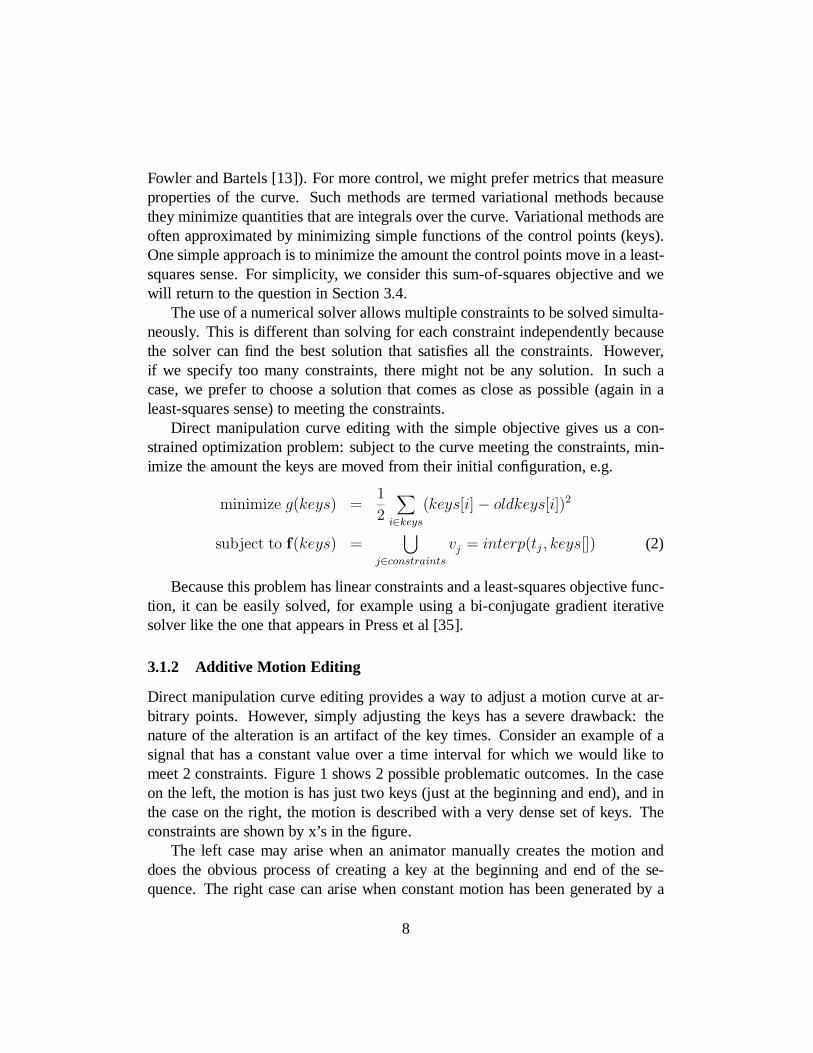
Direct manipulation curve editing provides a way to adjust a motion curve at ar-bitrary points. However, simply adjusting the keys has a severe drawback: thenature of the alteration is an artifact of the key times. Consider an example of asignal that has a constant value over a time interval for which we would like tomeet 2 constraints. Figure 1 shows 2 possible problematic outcomes. In the caseon the left, the motion is has just two keys (just at the beginning and end), and inthe case on the right, the motion is described with a very dense set of keys. Theconstraints are shown by x’s in the figure.

The left case may arise when an animator manually creates the motion anddoes the obvious process of creating a key at the beginning and end of the se-quence. The right case can arise when constant motion has been generated by a

8

A

B

C

D

E

Figure 1:

A

B

Editing a motion Curve.

Two straight line curves are to be adapted to pass through goals (denoted byX). The curve on the left has two keys, the curve on the right has many.

New keys are inserted into the curves so that the new goals are interpolated.

9

( )

( ) = ( []) + ( )

d t

p t interp t, keys d t ,

3.1.3 Additive Editing with Constraints

motion tracking system (providing a key at every frame). Such differences arrisebecause key spacing was determined for some reason other than later adaptation.Because editing the curve, by either inserting new keys or adjusting existing keys,depends on the key spacing, different results occur (Figure 1b and 1c).

Moving or inserting new keys edits the motion to meet new constraints, butoften does not provide the desired control. The actual change that occurs is depen-dent on how the curve was originally constructed, not on the users needs. Ideally,the user should be able to control the scope of the changes.

Motion displacement curves provide a solution to this problem. Rather thanediting the keys of the motion curve, which may be inconveniently placed, wemodify the curve by adding a new curve, to the motion so

and alter the parameters of this new curve instead. This provides freedom tochoose functions which alter the motion in desirable ways that do not depend onthe representation of the original signal.

Motion displacement maps are a successful variety of displacement curve.As introduced by Bruderlin and Williams [8] and Witkin and Popovic [46], themethod uses an interpolating spline for the displacement curve. The keys of thisspline can be placed at convenient locations to specify where changes are to oc-cur. By choosing the key spacing for the displacement curve appropriately, theanimator can have frequency control over the changes made to the motion. Thebottom of Figure 1 shows such a displacement curve, d, that allows us to get thedesired shape for both case A and case B.

Many other motion editing techniques can be viewed as variants of the dis-placement curve approach. For example, motion blending introduced by Bruderlinand Williams [8] and Perlin [33] uses another motion signal as the displacementmap. Common to all these approaches is the editing of a signal by adjusting theparameters of a secondary signal.

So far, we have reviewed two previous approaches to motion editing: constraint-based direct manipulation approaches, that provide freedom in specifying goalsto be met, and motion displacement mapping, that provides control over how mo-tions are affected. We introduce a novel technique that combine these two toprovide the controls of the former with the effects of the latter.

10

1

1

.qq

In the constrained optimization literature, the term “global” sometimes has a different mean-ing, refering to algorithms that guarantee the solution is not a local minimum. We do not use suchan algorithm.

The problem of motion editing with a displacement method involves findingvalues for the parameters of the displacement map. If we have some requirementsfor the resulting signal, this may be easy or difficult depending on the type offunction representing the displacement curve. For a displacement curve that isa spline with keys at the times of the constraints (as in [46]), determining therequired changes is easy. In other cases, it might be more difficult.

We could choose our displacement curve representation based on how easythe curve is to control, but we also must choose it based how the curve affectsthe motion. These can be conflicting goals: we might need a displacement mapcurve with distant keys to prevent adding high frequencies, but also need to placea number of constraints at nearby times, or we might want to choose a curve otherthan an interpolating spline for its smoothness properties. It is our premise thatflexibility in what types of displacement curves we choose is important, and theirdesign must be decoupled from our need for an effective interface.

Fortunately, we can provide convenient controls for any displacement curvesusing the direct manipulation curve techniques of Section 3.1.1. Rather than nec-essarily solving for new key values, we solve for the parameters of the displace-ment curve. As before, our solver provides minimum change solutions on under-determined problems, and least-squares-error solutions solutions for cases wheretoo many constraints have been specified so that no solution can meet them all.This provides a uniform interface to whatever type of displacement curve we de-sired, on the condition that the solver is capable of handling the equations.

The core of our method is to create a curve that is the summation of the originalmotion and displacement curves, specify constraints on these summed curves, andthen solve for the parameters of the displacement curve to achieve the goals. Wepose this as a single constraint problem over the whole motion. It is “global” inthe sense that the solution considers all constraints simultaneously, as opposed toconsidering each frame independently .

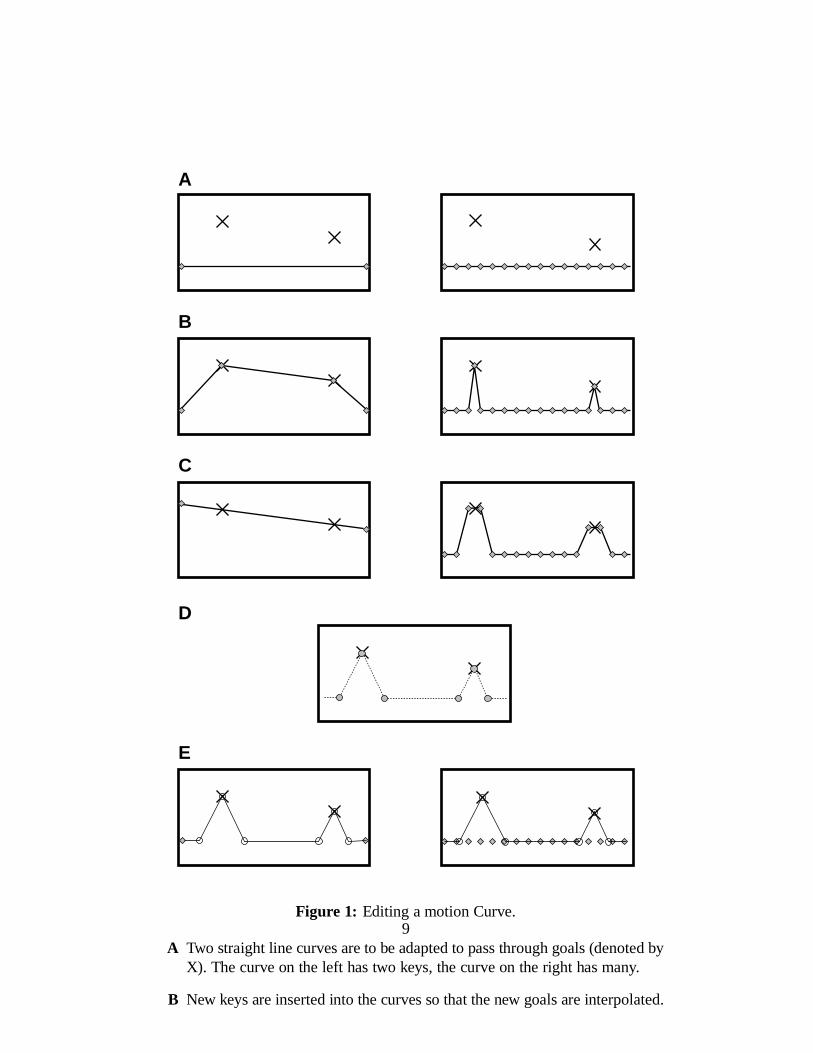
We denote the vector of parameters that are computed by the solver by Forediting a motion displacement curve, would be the parameters of the curve,for example, the concatenation of its control points. To illustrate this, we givethe trivial example shown in Figure 2. Here, we add a signal that is the linearinterpolation of 3 key values to an initial signal, and require that the 1st and lastkey have a zero value, which ensures that the motion connects at the ends. The

11

∗

i

i

q

p v

p

0

4

0 4

0

3.2 A Particle

( )

(4) + 75 =

( ) =

( ( )) =

p t .v ,

p . q v ,

p .

t ,

f t v.

parameter vector for this motion consists of the single value of the middle key.We denote the intitial motion as An example constraint might specify thevalue of the resulting curve at time 4 to be which leads to the constraint

where the .75 factor comes from the fact that frame 4 is 75% of the way betweena zero key and the key whose value is q. This constraint is independent of therepresentation for

Most graphical models have more than one parameter. We consider the simplest,a particle in 2D. To animate the particle, we need 2 motion signals (which we canview as a vector signal). All motion editing approaches in section 3.1 treated thesesignals independently.

With a constraint-based approach, we are able to handle all signals (or all theelements of a vector signal) simultaneously. This lets us place constraints on sig-nals that do not just depend on a single parameter. For example, we might wantour particle to be a specified distance away from a center point at a particular time.This doesn’t necessarily specify the particle’s location, it just places a constrainton it — for the example, the particle might lie anywhere on a circle surroundingthe centerpoint. Specifying the coordinates of the particle, which is all indepen-dent control of its parameters affords, may not be sufficient. For example thedistance constraint does not specify where on the circle the particle lies, the ex-act position may be determined by other things, such as other constraints or thelocation of the particle at other times.

Multi-parameter models require the ability to use a richer variety of constraintson the motion signals. Rather than simply being able to specify

we add the freedom to specify

The set of variables we must solve over, the state vector, is the concatenationof all of the parameters of the displacement curves for each parameter. The ma-chinery of the previous sections requires little alteration, except that the function

12

1Time

5432 9876

Val

ue

1Time

5432 9876

Val

ue

1Time

5432 9876

Val

ue

B)

A)

C)

0p .

Figure 2:

A

B

C

A trivial example of additive editing.

An initial signal,

A displacement curve that linearly interpolates 3 controls, denoted bysquares.

The final curve is the summation of the initial and displacement curves. Thevalue of the key of the displacement curve is computed such that the finalcurve passes through the constraint, denoted by the circle.

13

i

0 1

≥

∈ −

t t

t

t t

p

p

e f p

e f

p p

( ( ))

( [ ]) =

= ( )

3.3 A Character

f

f t v.

f t t t v.

,

t,

t.

is likely to be non-linear, which means we need a solver capable of handlingsuch equations. Another useful extension to the solver is to add the facility forinequality constraints such as

It is also desirable to be able to add constraints that are enforced over an inter-val of time

To solve such constraints in the continuous time domain requires solving varia-tional calculus problems. To approximate these using the machinery presented,we add an individual constraint for each frame in the time interval. For anima-tionsm this approximation is reasonable because the motion is only sampled atdiscrete frame times.

Most interesting animations require models that are more complicated than a par-ticle. For these problems the methods of the previous section still work, but thenumber of input variables and the set of useful constraints (and their complexity)grows.

Consider editing the motion of an articulated figure. The parameters of thisfigure are most likely to include a set of joint angles and a position for the rootof the hierarchy. We prefer not to specify these parameters directly. Instead, weprefer to control quantities of interest, such as the position of a hand. Since thisposition is a function of the model parameters, we can place a constraint on thehand by placing a constraint on the function which calculates the hand position.These constraints are identical to the constraints used with inverse kinematics,the difference being that rather than simply being used to compute the character’spose, the constraints serve to determine the entire motion.

Mathematically, an inverse kinematics constraint specifies

where is the desired position of the end-effector at time is the functionthat computes the position of the end-effector from the characters parameters (e.g.joint angles), and is the parameters for time For inverse kinematics, would

14

1

t 0

0

e f p d q

p d qq

t t, ,

t t, t,t ,

t

= ( ( ) + ( ))

( ) ( )

3.4 Sensitivity Scaling

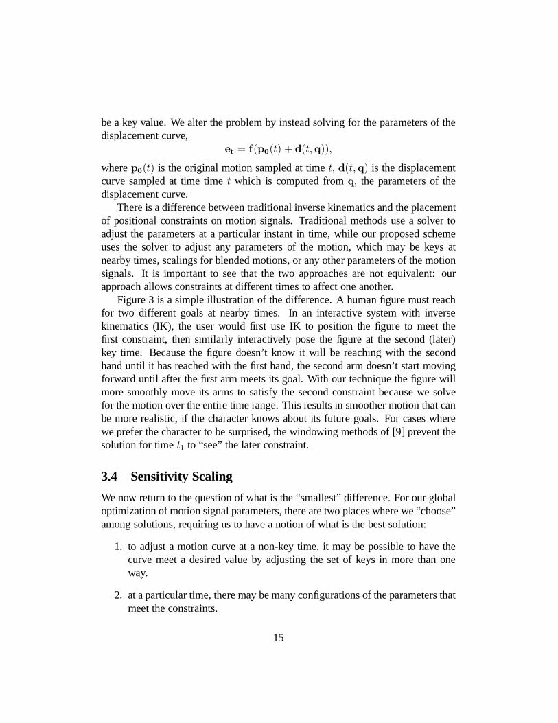
be a key value. We alter the problem by instead solving for the parameters of thedisplacement curve,

where is the original motion sampled at time is the displacementcurve sampled at time time which is computed from the parameters of thedisplacement curve.

There is a difference between traditional inverse kinematics and the placementof positional constraints on motion signals. Traditional methods use a solver toadjust the parameters at a particular instant in time, while our proposed schemeuses the solver to adjust any parameters of the motion, which may be keys atnearby times, scalings for blended motions, or any other parameters of the motionsignals. It is important to see that the two approaches are not equivalent: ourapproach allows constraints at different times to affect one another.

Figure 3 is a simple illustration of the difference. A human figure must reachfor two different goals at nearby times. In an interactive system with inversekinematics (IK), the user would first use IK to position the figure to meet thefirst constraint, then similarly interactively pose the figure at the second (later)key time. Because the figure doesn’t know it will be reaching with the secondhand until it has reached with the first hand, the second arm doesn’t start movingforward until after the first arm meets its goal. With our technique the figure willmore smoothly move its arms to satisfy the second constraint because we solvefor the motion over the entire time range. This results in smoother motion that canbe more realistic, if the character knows about its future goals. For cases wherewe prefer the character to be surprised, the windowing methods of [9] prevent thesolution for time to “see” the later constraint.

We now return to the question of what is the “smallest” difference. For our globaloptimization of motion signal parameters, there are two places where we “choose”among solutions, requiring us to have a notion of what is the best solution:

1. to adjust a motion curve at a non-key time, it may be possible to have thecurve meet a desired value by adjusting the set of keys in more than oneway.

2. at a particular time, there may be many configurations of the parameters thatmeet the constraints.

15

TraditionalInverse

Kinematics

GlobalOptimizationfor 4 evenly-spaced keys

Frame 0 Frame 6 Frame 9 Frame 1

Figure 3: An articulated figure reaches for two points.An articulated figure is instructed to grab the first dot at time 6 and the seconddot at time 9 of a 16 frame animation. Frames 0, 6, 9 and 15 are shown for two

different methods. In the upper sequence, traditional inverse kinematics are usedto position the figure to meet the goals. Because the constraints are solved

indepently, they do not take each other into consideration. In the lower sequence,our method is used with a displacement curve that uses cubic interpolation on 4evenly spaced keys. Notice how the character "plans ahead" by starting to movetowards its later goal (look at the position of the non-grabbing hand in frame 6).

16

2−

·

∑∑

∑∑

i j ij

ij

ijt p

p p

1( [ ][ ] [ ][ ])

=( )

[ ][ ]

( )

[ ][ ]

wkeys i j oldkeys i j ,

w j i.

w∂f t

∂keys i j

∂f t

∂keys i j,

t p

As we mentioned in Section 3.1.1, the simplest approach to constraint-basedcurve editing is to minimize the amount of change in the keys. Such an approachis undesirable because each parameter may affect the resulting animation by adifferent amount. For example,

1. if a signal is created by linearly interpolating between keys at time 0, 5, 10and 100, an adjustment of key 5 will cause a much smaller change to theresulting animation than a similar change at key 10, because changing key5 will affect a much smaller interval of time;

2. an adjustment to the character’s hand angle will make much less of a differ-ence than a similar adjustment to the torso, because changing the torso willaffect a large part of the body (including the hand);

3. an adjustment of equal numerical magnitude in parameters that are mea-sured in different units, for example millimeters and miles, will have wildlydifferent effects. Comparison between units can be especially difficult whenthe two parameters do not measure similar quantities, such as meters and ra-dians.

All of these issues can be addressed by choosing an optimization criterionthat minimizes a measure of how much the resultant animation changes, ratherthan just how much the parameters change. This criterion offers a mechanism fordefining the kinds of effects various manipulations will have. Currently, we usea weighted least squares metric, as described in [16]. Rather than minimizing themagnitude of the parmeter changes (as in Equation 2), we weight the least squares,giving each individual scalar variable a different weight. That is, we minimize

where is a weighting factor for variable of key We pick the weights suchthat each of the variables that we control have the same effect. For example, bycomputing

which computes a weight for each variable that computes the sum (over all timesin the animation and points on the character) of the magnitude of the change

on the animation due to the variable.

17

•

•

•

•

•

•

3.5 A Menagerie of Constraints

3.6 Comparison with other constraint-based methods

The least-squares weighting approximates the objective function that measuresthe difference between the original and resulting animation, measured by the po-sitions of points on the characters. Because of the numerical methods that we willuse in Section 4.1, we would need to create a quadratic approximations to the non-linear objective function. The weights are the diagonal elements of a quadraticapproximation to this objective. The quality of the approximation is unimportant,because it is unclear how useful the real objective would be. We propose otherobjective functions in Section 6, and typically rely on using additional constraintsand well designed motion representations, rather than on the objective funtion, tocontrol our results,

Although we have not experimented extensively with varying optimization objec-tives to control the resulting motion, we have employed a variety of constraintsboth to specify our requirements for the resulting motion, and to guide the solverto motions that we prefer. With our general non-linear solver, many constraintsare possible (see [44] or [16] for some examples of the utility of the generalityof non-linear constraints). Some constraints that we have used in our examplesinclude:

constrain a point to be a particular place at a particular time;

constrain a point to be above the floor;

constrain a point to be at another point’s location at a particular time;

constrain a point to follow another point’s motion path;

constrain two points to have a particular distance (at a particular time orover a range of times);

constrain an angle between two vectors to be within a range of values (goodfor joint limits).

Like many other approaches in computer graphics and animation, we use numeri-cal constraint solving to provide a convenient set of controls. As we mentioned in

18

4.1 Solver

4 Implementation

Section 2, most constraint methods perform solving for individual times, with thenotable exception of spacetime constraint methods.

Our method is a variant of the spacetime motion synthesis approach pioneeredby Witkin and Kass [45] and Cohen [9]. We use a similar set of constraints,and similar implementation techniques. The fundamental difference between theprevious methods and ours is that we do not necessarily generate physical motions,but instead adapt pre-existing motions. For this reason we do not need to includethe constraints that insure physical motion, do not need to pose our problems ascontrol instead of placement, and choose objective functions based on motionsimilarity rather than energy optimality. We believe that this eliminates many ofthe concerns that hinder the spacetime approach: it is simpler to implement (sincewe do not need to derive equations of motion), constraint solving is more tractable,it is applicable across a broader domain (not just physically correct motions), andit is potentially easier to use (picking a motion seems a more reasonable task thandesigning a physical control system).

One issue that we share with the previous spacetime constraint approaches is thatwe must set up large, complex constrained optimization problems. How this isaccomplished is not important to the method — in fact, we would prefer to hide itas much from the user as possible. What is important is that the methods are fast,robust and that the problems can be defined on the fly in response to the user’srequests. We therefore only describe implementation strategies briefly.

Our methods rely on the use of a solver for non-linear constrained optimizationproblems. Good, general methods for such problems are an unsolved problem.Press et al [35] argues that not only does no reliable, general, non-linear solverexist, but that one cannot exist. The difficulty of the general problem has lead toan extensive literature and a wide variety of methods. (we suggest textbooks byFletcher [12] or Gill et al [14], or the general numerical analysis text by Press etal [35] for a practical introduction).

Non-linear constraint solving has been used in many computer graphics appli-cations, such as inverse kinematics. Solvers used this way are applicable to theproblems of our methods with some extensions:

19

+

g

,

•

•

•

≥e e

i i

i i 1

q qMq

f q c

f q c

M qf q

M

q q

minimize ( ) =1

2subject to ( ) =

( )

( )

sequential quadratic programming

active set

a

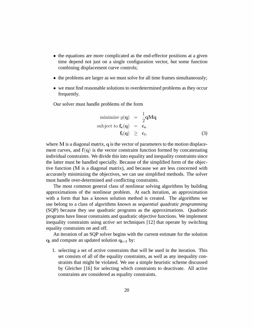
the equations are more complicated as the end-effector positions at a giventime depend not just on a single configuration vector, but some functioncombining displacement curve controls;

the problems are larger as we must solve for all time frames simultaneously;

we must find reasonable solutions to overdetermined problems as they occurfrequently.

Our solver must handle problems of the form

(3)

where is a diagonal matrix, is the vector of parameters to the motion displace-ment curves, and is the vector constraint function formed by concatenatingindividual constraints. We divide this into equality and inequality constraints sincethe latter must be handled specially. Because of the simplified form of the objec-tive function ( is a diagonal matrix), and because we are less concerned withaccurately minimizing the objectives, we can use simplified methods. The solvermust handle over-determined and conflicting constraints.

The most common general class of nonlinear solving algorithms by buildingapproximations of the nonlinear problem. At each iteration, an approximationwith a form that has a known solution method is created. The algorithms weuse belong to a class of algorithms known as(SQP) because they use quadratic programs as the approximations. Quadraticprograms have linear constraints and quadratic objective functions. We implementinequality constraints using techniques [12] that operate by switchingequality constraints on and off.

An iteration of an SQP solver begins with the current estimate for the solutionand compute an updated solution by:

1. selecting a set of ctive constraints that will be used in the iteration. Thisset consists of all of the equality constraints, as well as any inequality con-straints that might be violated. We use a simple heuristic scheme discussedby Gleicher [16] for selecting which constraints to deactivate. All activeconstraints are considered as equality constraints.

20

≈

−

i i

i

i i

i

i i iT

i

i

i

i

∂

∂,

∂ /∂.

,

.

g g

,

κ κ

4.2 Setting up systems

( + ) ( ) +

= ( ) =

( + ) = ( ) + +1

2

+

+

f q ∆ f qf

q∆

f q qJ

J∆ c f q c

c

∆

q ∆ q q M∆ ∆ M∆

q M∆

∆q ∆

q ∆

q

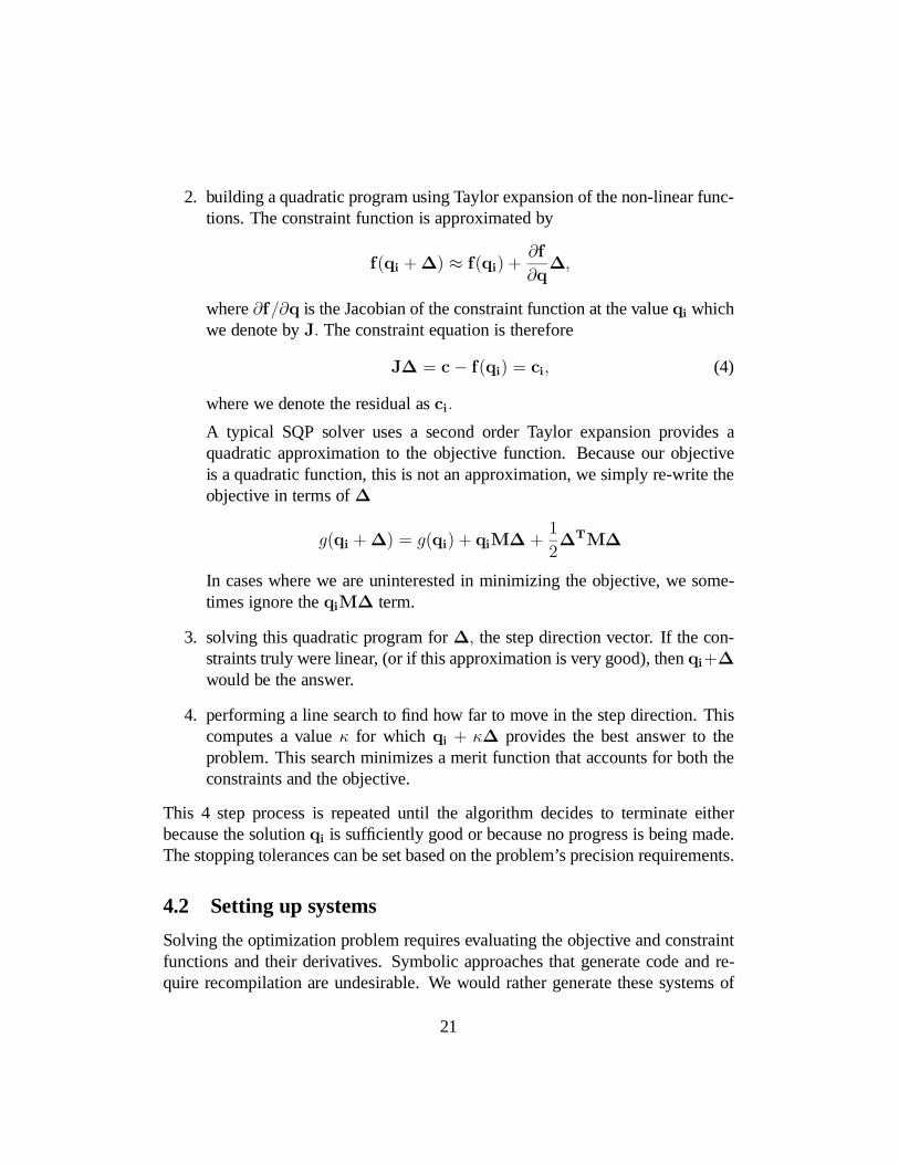
2. building a quadratic program using Taylor expansion of the non-linear func-tions. The constraint function is approximated by

where is the Jacobian of the constraint function at the value whichwe denote by The constraint equation is therefore

(4)

where we denote the residual as

A typical SQP solver uses a second order Taylor expansion provides aquadratic approximation to the objective function. Because our objectiveis a quadratic function, this is not an approximation, we simply re-write theobjective in terms of

In cases where we are uninterested in minimizing the objective, we some-times ignore the term.

3. solving this quadratic program for the step direction vector. If the con-straints truly were linear, (or if this approximation is very good), thenwould be the answer.

4. performing a line search to find how far to move in the step direction. Thiscomputes a value for which provides the best answer to theproblem. This search minimizes a merit function that accounts for both theconstraints and the objective.

This 4 step process is repeated until the algorithm decides to terminate eitherbecause the solution is sufficiently good or because no progress is being made.The stopping tolerances can be set based on the problem’s precision requirements.

Solving the optimization problem requires evaluating the objective and constraintfunctions and their derivatives. Symbolic approaches that generate code and re-quire recompilation are undesirable. We would rather generate these systems of

21

· · ·

h

h

h

h

h 0 1 n

i

t

t,

∂

∂

∂

∂

∂

∂.

∂ /∂ ,

,

x

( ) = ( ( ))

=

( ) = ( ) ( ) ( )

4 4

automatic differentiation

f x e p q

ep

f

q

e

p

p

q

e p

e x M x M x M x h

M h

equations on the fly in response to user interactions. Thus, we use an approachfirst introduced by Witkin and Kass [45] and further developed and encapsulatedby Gleicher and Witkin [18]. This snap-together-math system provides data struc-tures that represent functional elements that are “wired together” with composi-tion. We extend this idea to wire together entire motions, allowing us to buildconstraint problems using primitives such as interpolation of keys and time warpsin addition to more basic mathematical functions.

The constraint and objective functions for the motion adaptation problems canbe large and complicated: they involve the blending of keys, the kinematics ofthe character, and the relation applied to these points. Viewed as a monolithicwhole, these functions are daunting. However, viewed as smaller pieces composedtogether, the task is much more manageable. The derivatives of these composedfunctions can be built by the chain rule. Rather than symbolically performing theprocess, the elements are computed and multiplied together numerically, a processcalled [19]. For example, a constraint of the position ofthe hand of an articulated figure at time might have the form

where is the kinematic function that computes the position of the hand giventhe figure’s parameters, and is the function that computes the parameters at agiven time from the key configuration. The chain rule permits us to compute

Each of the two matrices can be computed independently and multiplied together.We use a general purpose implementation of automatic differentiation [16] [18]designed specifically for the demands of interactive systems, allowing functionsto be defined dynamically and evaluated efficiently.

To compute the Jacobian of the kinematic function we also use amixed symbolic-numeric approach. The kinematics is defined by a chain of matrixmultiplications. We compute the Jacobian by recursively applying the product rulefor differentiation, symbolically computing the derivatives of each transformationbut combining them numerically.

where each is a function that computes a transformation matrix andis the position of the end effector in its local coordinate frame. The Jacobian

22

· · ·+ +

++

+

i

∂

∂

∂

∂

∂

∂

∂.

∂ /∂

g

i 1 i 1 n

i i i 1 ii 1 i

i 1

i

T

i

h M M h

m

x

M h

x

M

xh M

h

x

M x

∆ ∆ M∆

f ∆ J∆ c

M

4.3 Solving the Quadratic Program

+ 1=

= = +

minimize ( ) =1

2subject to ( ) = =

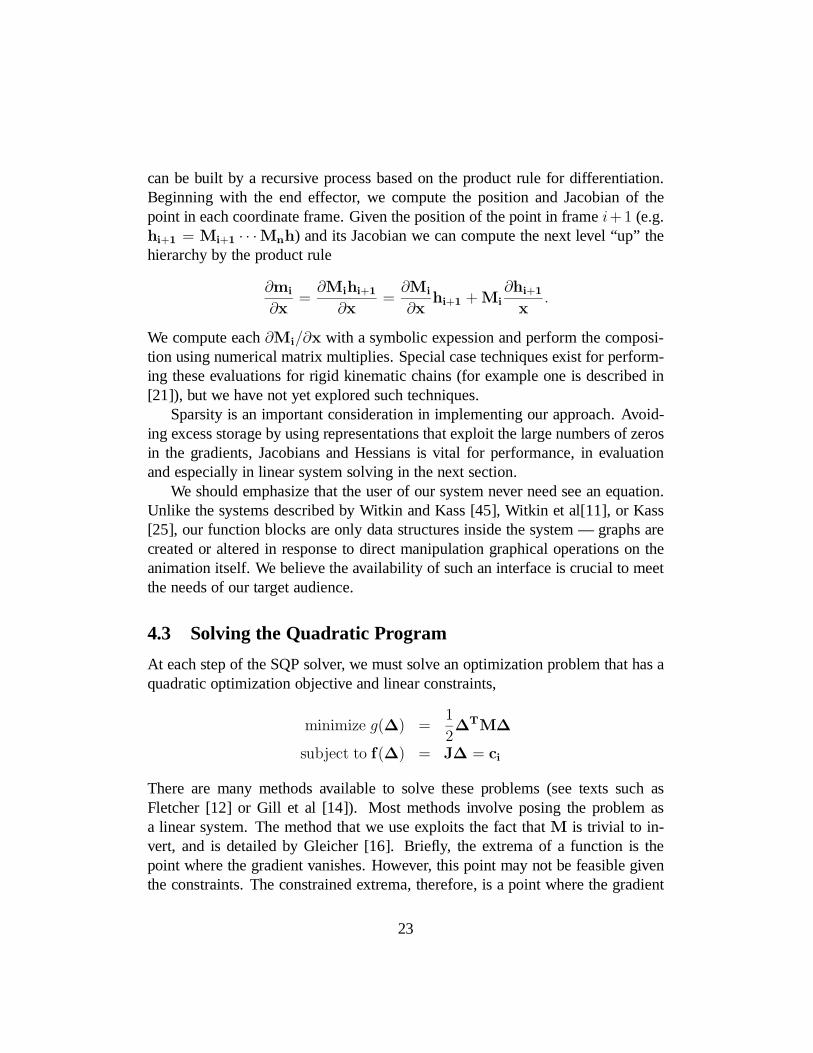
can be built by a recursive process based on the product rule for differentiation.Beginning with the end effector, we compute the position and Jacobian of thepoint in each coordinate frame. Given the position of the point in frame (e.g.

) and its Jacobian we can compute the next level “up” thehierarchy by the product rule

We compute each with a symbolic expession and perform the composi-tion using numerical matrix multiplies. Special case techniques exist for perform-ing these evaluations for rigid kinematic chains (for example one is described in[21]), but we have not yet explored such techniques.

Sparsity is an important consideration in implementing our approach. Avoid-ing excess storage by using representations that exploit the large numbers of zerosin the gradients, Jacobians and Hessians is vital for performance, in evaluationand especially in linear system solving in the next section.

We should emphasize that the user of our system never need see an equation.Unlike the systems described by Witkin and Kass [45], Witkin et al[11], or Kass[25], our function blocks are only data structures inside the system — graphs arecreated or altered in response to direct manipulation graphical operations on theanimation itself. We believe the availability of such an interface is crucial to meetthe needs of our target audience.

At each step of the SQP solver, we must solve an optimization problem that has aquadratic optimization objective and linear constraints,

There are many methods available to solve these problems (see texts such asFletcher [12] or Gill et al [14]). Most methods involve posing the problem asa linear system. The method that we use exploits the fact that is trivial to in-vert, and is detailed by Gleicher [16]. Briefly, the extrema of a function is thepoint where the gradient vanishes. However, this point may not be feasible giventhe constraints. The constrained extrema, therefore, is a point where the gradient

23

·1 2

−

−

−

λ

λ

λ

λ

λ

λ

T

1 T

1 Ti

i

1 Ti

4.4 Line Search

g

,

,

, , ,.

ε ,

ε

e α g α

=

=

=

( + ) =

( ) = ( ) + ( ) ( )

Lagrange Multipliers

M∆ J

∆

∆ M J

JM J c

c G J∆

JM J I c

I

∆∆

x x f x f x

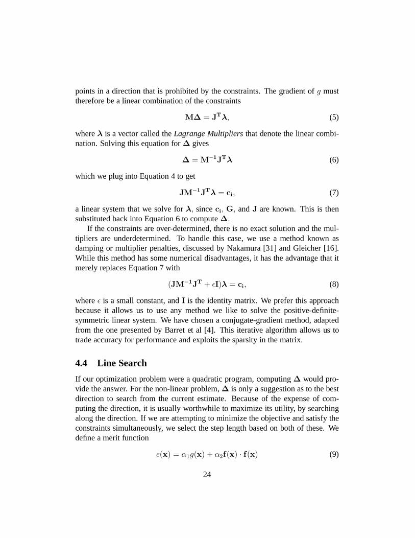
points in a direction that is prohibited by the constraints. The gradient of musttherefore be a linear combination of the constraints

(5)

where is a vector called the that denote the linear combi-nation. Solving this equation for gives

(6)

which we plug into Equation 4 to get

(7)

a linear system that we solve for since and are known. This is thensubstituted back into Equation 6 to compute

If the constraints are over-determined, there is no exact solution and the mul-tipliers are underdetermined. To handle this case, we use a method known asdamping or multiplier penalties, discussed by Nakamura [31] and Gleicher [16].While this method has some numerical disadvantages, it has the advantage that itmerely replaces Equation 7 with

(8)

where is a small constant, and is the identity matrix. We prefer this approachbecause it allows us to use any method we like to solve the positive-definite-symmetric linear system. We have chosen a conjugate-gradient method, adaptedfrom the one presented by Barret et al [4]. This iterative algorithm allows us totrade accuracy for performance and exploits the sparsity in the matrix.

If our optimization problem were a quadratic program, computing would pro-vide the answer. For the non-linear problem, is only a suggestion as to the bestdirection to search from the current estimate. Because of the expense of com-puting the direction, it is usually worthwhile to maximize its utility, by searchingalong the direction. If we are attempting to minimize the objective and satisfy theconstraints simultaneously, we select the step length based on both of these. Wedefine a merit function

(9)

24

+i

1

x ∆α κκκ,

5 Examples

5.1 Jumping

that evaluates the quality of a solution. In cases where we are not concerned withthe objective, we often set to 0. We find a value of the step length thatfor which the new value minimizes the merit function. The line searchprocess tries various values of evaluating the merit function for each. We use avariant of Brent’s method [35] to perform the line search.

There is a tradeoff between spending effort on computing step directions andon making evaluations in the line search. For problems such as ours, some linesearching is useful because evaluations are much less costly than computing newstep directions.

We now consider a number of examples to illustrate our approach. All were cre-ated using our prototype system. In cases where prior approaches are shown forcomparison, these approaches have been implemented in our system. For many ofthe examples, we include solution times on a Power Macintosh 8500. For most ofthe examples, the character being animated is a stick figure with 12 joint angles, aposition for the pelvis, and 12 limb lengths which are not permitted to vary in anyof the presented examples. Unless otherwise noted, we use cubic interpolationand the objective function using sensitivity scaling described in Section 3.4.

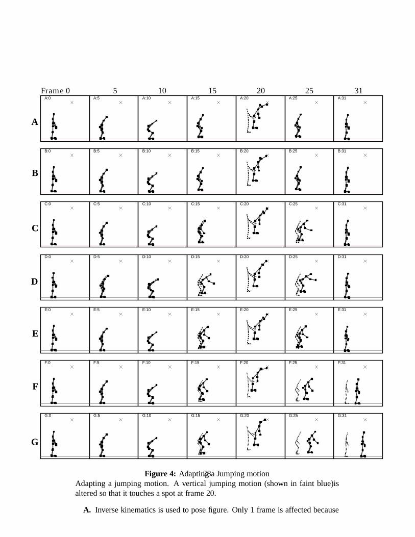
For out first example, we consider altering a jumping motion to meet a desiredgoal. An animator provided us with a motion of a stick figure jumping. We wouldlike to alter this motion such that the character touches a particular point (denotedby the small cross) at a particular time (frame 20 of the 32 frame sequence). Theuser can specify this single constraint of this example interactively. The only otherthing which must be specified is the type of displacement curve. Figure 4 showsresults for a variety of displacement curves, and Figure 5 shows a graph of the Xcoordinate of the pelvis (the root of the hierarchy).

Figure 4a shows an attempt to use traditional inverse kinematic keyframe edit-ing on the sequence (e.g. no displacement curve). Dragging the position of thehand at time 20 is easy, and provides a good result for this frame. However, be-cause the original motion has a key for every frame of the motion, the alterationonly affected one frame, failing to create an acceptable motion.

25

xx

x

x

Figures 4b and 4c show the use of the previous motion displacement technique[46] [8]. The displacement curve has a key at time 20 whose value is computedwith inverse kinematics. Two additional zero valued keys limit the effect of thealteration. In Figure 3b, we simply chose to place the new keys 5 frames from theedited key (so there are two zero keys at times 15 and 25, and the constraint key attime 20). In Figure 3c, we place the keys at the takeoff and landing points of thejump so only the flight of the jump is affected (zero valued keys at times 13 and29). This, in effect, broadened the scope of the change, and introduced unevenkey spacing for the displacement curve.

Figure 4d shows the use of our method on our system’s default displacementcurve with 5 evenly spaced keys over the entire motion. Figure 4e shows a curvewith 4 keys evenly spaced only over the time of the jump.

While the creation of Figure 4d and Figure 4e require the generality of ourmethod, it admittedly provides little advantage in this case. The motions are allsimilar enough that none is definitively best. A subjective poll of some colleaguesdidn’t result in a consistent preference. However, several people complained noneseemed realistic because the character is pulled back to the original position, as ifconnected to the left edge of the frame by a rubber band. We could correct thisproblem by placing a constraint on the final position of the character, although thiswould require us to know the length of the jump. We can also correct this flaw bychoosing a different displacement map.

Figure 4f and Figure 4g show the use of our method with a ”contrived” dis-placement map. We wish to have the character move continuously in the direc-tion throughout its flight. To enforce this, we use a displacement curve for theposition of the pelvis that has only two keys — one at the beginning of the flightand one at the end. We permit only the end key to be altered. If the charactermoves forward while jumping, it must do so continuously across the flight. Withour objective function, altering this last key of the position curve causes more ofa change to the animation than other variables because it effects a larger time in-terval. Due to this, the solver will prefer to change it less than the other variables,resulting in a shortened jump. Manually adjusting the weight on the variable forthe displacement key adjusts the length of the jump (Figure 4g).

Developing the contrived displacement curve of the last paragraph is beyondthe skills of much of our potential audience, but so would manually tweaking themotion to generate a good jump. While it did take effort to devise the curve, itis reusable: we could place different constraints on the jump and solve again. Ineffect, we have created a procedure for creating goal-directed jumping motions.When the effort to devise the displacement map is compared to approaches for

26

5.2 Hand Gestures

5.3 Walking

generating paramterized motion, the approach seems more reasonable.We emphasize that for this example, we merely took an existing motion and

added a single constraint. The only other thing specified was the type of the inter-polating curve used for the displacement. Each variant described can be createdby specifying a different displacement map. Solution times for all were less thana quarter of a second.

To show the advantages of solving the inverse kinematics problems on the dis-placed motion we consider a simple example with two initial motions. We beginwith a stick figure standing still, and a point which moves in a square path (linearinterpolation between the corner points). We would like the character to trace thepath of the point with its hand. In Figure 6a the motion is generated by solvingthe inverse kinematics problem independently for each frame. This motion accu-rately tracks the square, but is not smooth — in fact, it contains “jigglies” wherethe elbow alternates between solutions where the elbow is either straight or bent.In Figure 6b, motion displacement maps [46] are used, placing a displacementkey at the corners of the square and solving the inverse kinematics at these 5 keysto determine their values. This creates a motion that is smooth, but does not ap-proximate the square well. In contrast, Figure 6c shows the use of our methodsapplying a pseudo-variational constraint that ties the figure to the moving point.Because we have chosen a cubic displacement curve with only 5 keys, the figurecannot track the square exactly. However, it gets as close as possible given thelimitations. To better approximate the path, a displacement curve with more keyscan be used.

To solve this problem we placed two constraints: one ties the hand to a givenmotion path, and one keeps the pelvis stationary. Our system then generates apositional constraint for the pelvis and hand at each of the 21 frames. Each po-sitional constraint is 2 scalar constraints, so this results in 2 x 2 x 21 = 84 scalarconstraints.

In this section, we consider adapting a 2D walking motion obtained by rotoscop-ing video of one of the author’s walking. This latter point is significant for com-parison with alternate approaches such as synthesis. Our goal in adapting thismotion is to obtain new motions that maintain as much of this walk as possible:

27

G:0 G:5 G:10 G:15 G:20 G:25 G:31

F:0 F:5 F:10 F:15 F:20 F:25 F:31

E:0 E:5 E:10 E:15 E:20 E:25 E:31

D:0 D:5 D:10 D:15 D:20 D:25 D:31

C:0 C:5 C:10 C:15 C:20 C:25 C:31

B:0 B:5 B:10 B:15 B:20 B:25 B:31

A:0 A:5 A:10 A:15 A:20 A:25 A:31

Frame 0 5 10 15 20 25 31

A

B

C

D

E

F

G

Figure 4:

A.

Adapting a Jumping motionAdapting a jumping motion. A vertical jumping motion (shown in faint blue)isaltered so that it touches a spot at frame 20.

Inverse kinematics is used to pose figure. Only 1 frame is affected because

28

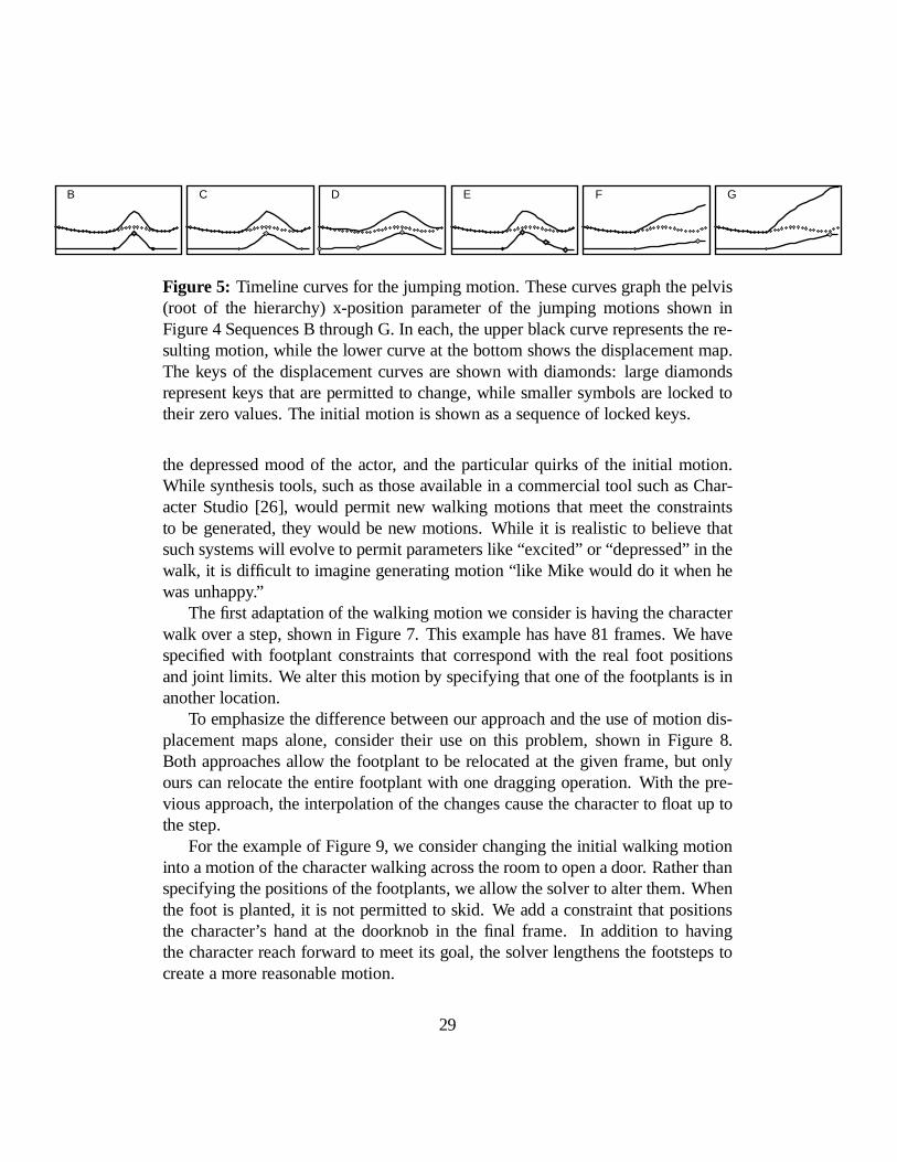
B C D E F G

Figure 5: Timeline curves for the jumping motion. These curves graph the pelvis(root of the hierarchy) x-position parameter of the jumping motions shown inFigure 4 Sequences B through G. In each, the upper black curve represents the re-sulting motion, while the lower curve at the bottom shows the displacement map.The keys of the displacement curves are shown with diamonds: large diamondsrepresent keys that are permitted to change, while smaller symbols are locked totheir zero values. The initial motion is shown as a sequence of locked keys.

the depressed mood of the actor, and the particular quirks of the initial motion.While synthesis tools, such as those available in a commercial tool such as Char-acter Studio [26], would permit new walking motions that meet the constraintsto be generated, they would be new motions. While it is realistic to believe thatsuch systems will evolve to permit parameters like “excited” or “depressed” in thewalk, it is difficult to imagine generating motion “like Mike would do it when hewas unhappy.”

The first adaptation of the walking motion we consider is having the characterwalk over a step, shown in Figure 7. This example has have 81 frames. We havespecified with footplant constraints that correspond with the real foot positionsand joint limits. We alter this motion by specifying that one of the footplants is inanother location.

To emphasize the difference between our approach and the use of motion dis-placement maps alone, consider their use on this problem, shown in Figure 8.Both approaches allow the footplant to be relocated at the given frame, but onlyours can relocate the entire footplant with one dragging operation. With the pre-vious approach, the interpolation of the changes cause the character to float up tothe step.

For the example of Figure 9, we consider changing the initial walking motioninto a motion of the character walking across the room to open a door. Rather thanspecifying the positions of the footplants, we allow the solver to alter them. Whenthe foot is planted, it is not permitted to skid. We add a constraint that positionsthe character’s hand at the doorknob in the final frame. In addition to havingthe character reach forward to meet its goal, the solver lengthens the footsteps tocreate a more reasonable motion.

29

A B C

CBA

a

b

c

( )

( )

( )

Figure 6: An articulated figure’s hand is tied to a moving point that traces asquare point. The dotted line shows the path actually traced by the character’shand, and the lower pictures show the character’s position strobed from time 5to 10. Inverse kinematics applied to each frame individually. Although thecharacter traces the path precisely, the motion is “jiggly.”Note that the arm oscil-lates between being bent and straight. prior motion displacement techniquesare used, with displacement keys set with inverse kinematics at the four corners.This figure uses an interpolating cubic spline with 5 keys. Our method with 5keys for the displacement map and a variational constraint tying the hand to thesquare motion path. The resulting motion is smooth and approximates the square.Because the displacement has limited degrees of freedom, the square cannot betraced perfectly. This figure also uses an interpolating cubic spline with 5 keys. Adisplacement curve with more keys would produce a curve that better traced thepath.

30

Figure 7:

Figure 8 goes here

Figure 8:

A walking motion is shown on the left by “strobing.” The initial walk-ing motion is shown on the left. The character is made to step over an obstacle bychanging the location of the footplant constraint. The arrowed path shows wherethe footplant has been dragged.

The example of Figure 7 is detailed. The left shows the use of ourmethod to relocate the step. Notice that the footplant constraint is maintained asits position is moved. On the right, standard motion displacement mapping tech-niques are applied to adjust the footstep’s position at a frame. The method doespermit the user to reposition the foot and provides a smooth transition, however,because it only considers constraints on one frame, the techniques achieve the editby making the character float into the new place.

31

Figure 9:

5.4 Switching characters

The first 55 frames of the walking motion of Figure 7 are adapted tohave the character reach for a spot in the last frame. In this example, the solver ispermitted to adjust the footplant positions. The dotted figures represent the orig-inal motion, the arrows indicate the single constraint dragging operation. Noticethat positioning the characters hands not only causes him to lean forward but totake larger steps as well.

This example of Figure10 starts with two base motions: short and tall figureswalking. We wish to make the short man walk in the tall man’s footsteps. Theperiod of the footfalls match by design. However, if they didn’t, we could makethem match by using the dynamic time-warping algorithm presented by Bruderlinand Williams [8]. The constraints provided to our method were:

1. tie the x-position of the short figure’s torso to that of the tall figure;

2. make the short figure’s footpaths (specifically, the ankles) follow the tallerfigure’s foot paths;

3. maintain realistic joint angles (the arms, knees, feet and hands can’t bendbackwards);

4. maintain all body parts above the floor.

This example shows how the presented algorithm is used to modify an originalmotion so that end-effectors meet user-supplied goals, while retaining much of theoriginal character of the motion. Figure 10d shows the resulting motion. Figure

32

2

2

5.5 3D Examples

6 Discussion, Conclusions and Future Directions

In fact, the technique has not been demonstrated in the simpler, 2D case.

10e shows a similar example, the only difference being that for our initial motionwe have the short figure running. The footfalls of the tall character are largeenough that it is a stretch for the small character to meet them.

Thus far, we have demonstrated our approach with 2D examples. We note, how-ever, that there is nothing about our approach that precludes the more interest-ing case of 3D character animation. The basic elements of our approach havebeen demonstrated in 3 dimensions, both spacetime constraints [9] and motiondisplacement mapping [8] [46]. The system described in this paper has been ex-tended for 3D character animation [17]. An illustration of this is shown in Figure11, where a 3D motion of a walking character obtained by optical motion captureis altered by repositioning footplant constraints.

The most unique challenges in employing our constraint-based approach tomotion editing to 3D tasks are in the user interface. Specifying and visualizing thechanges to the 3D motions are a difficult task, especially in the constraint-basedapproach where a given frame might be affected by constraints on other frames,and similarly, each constraint may affect a number of frames on the motion. Thereare some potential technical challenges as well, for example, the quaternion repre-sentation typically preferred for 3D rotations does not have the addition operatordefined, therefore their use in a motion-displacement approach is non-trivial.

In this paper, we have presented a constraint-based approach to motion adaptation.With these methods, we can specify a set of goals that a motion needs to meet, andhave a pre-existing motion adapted to meet these needs in a way that preserves theinitial motion. Such methods can empower users without animation skill, allowingthem to create animations by selecting motions from libraries. The methods alsoenable scenarios where motions are created on the fly, without the intervention ofan animator.

In the course of developing our prototype implementation, experimenting withit on a number of examples, and assessing the methods, we have identified a num-ber of issues that might be better addressed:

33

A

B

C

D

E

Figure 10:

A.

B.

C.

D.

E.

Switching characters by constraint-based motion adaptation. Walkingmotions are shown for a tall character and a short character by strobing every 5frames in alternating shades of grey.

The initial walking motion of a tall character.

Initial walking motion of the small character.

Initial running motion for the small character.

Adapting the short character’s walk (B) to meet the footplants of the tallercharacters walk (A).

Adapting the short character’s run (C) to meet the footplants of the tallercharacters walk (A).

34

Figure 11 goes here

Figure 11: Visualizing a spacetime constraint-based motion edit of a walkingmotion. Strobing (with color alternation and transparency to help contend withclutter) and streamers (the thin lines following the feet and hand) are used to con-vey the motion. The striped streamer shows the initial (pre-edit) motion. Yellowsymbols represent constraints.

35

Usability

Objective Functions

Performance

Robustness

— Our approach offers advantages in that it allows the use of conve-nient constraint-based controls, like inverse kinematics. However, it alsorequires a variety of new control types to adjust the motions. To achieve adesired motion, one may need to change the key spacing or function typefor the displacement curve, select an alternate initial motion, or adjust theparameters of the objective function. We selected displacement curve typesempirically — we typically would try one or two of the default choicesand pick the motion we liked best. A good interface which allows definingmore complicated functions or key spacings for the displacement curves isan open question.

We believe that choosing an initial motion is an intuitive control over theresulting motion. As seen in the examples, we can pick initial motions withproperties that we want to see in the final animation.

— The choice of objective function provides a way to con-trol the types of motions the solver will find. To date, our emphasis hasbeen on specifying better motions through increased constraints. How-ever, Witkin and Kass [45] suggest how proper choice of objective functionsmight translate into high level goals. While objective like “as cautiously aspossible” seem out of reach for current methods, basic hints such as mak-ing the solver prefer to keep the knees bent or the figure balanced, could beadded to our system, although may prove difficult to present to users.

Better objective functions can also simplify the problem of choosing rep-resentations for the displacement curves. If the objective is well tuned todesireable motions, for example to prefer smooth displacements, there isless of a need for the displacement function to provide the preferences.

— On simple examples, our prototype is capable of providing real-time, direct manipulation with feedback. The user can drag a single frameand continuously see the changes made to the entire motion. Faster hard-ware and more sophisticated implementation techniques might make suchinteractions possible for more complicated problems.

— Solving general non-linear constrained optimization problems isan intractable problem. Any method we use cannot guarantee solving everyproblem we pose. So far, we have had good results with a relatively sim-ple solver. Better ones are both publicly and commercially available. Weare less concerned, however, with cases where our solver cannot find any

36

References

Acknowledgements

The Visual Computer

Time-dependent constraints and objectives

[1] William Armstrong and Mark Green. The dynamics of articulated rigid bodies forpurposes of animation. , 1:231–240, 1985.

solution, and more concerned with cases where the solver finds a correctsolution that is not the desired motion. Usually, this requires better specifi-cation of the problem, by adding more constraints or providing other hintsto the solver.

— We could add constraints andmetrics that compute functions of the motion, rather than the configura-tions. For example, we might place a limit on the velocities of a point, orprefer that a point follow a smooth path. Such functions would depend ona number of adjacent frames. Requiring that a point follow a physicallyvalid path seems to be a special case of this, which offers the potential ofintegrating our methods with traditional spacetime methods.

In conclusion, we have described a method which extends previous work onmotion editing by combining motion warping with constraint satisfaction, result-ing in a system that provides retention of the original qualities of a motion whilemapping it into a new scene or onto a new character. This technique will empowerthe novice animator, and provide better starting motion for the experienced anima-tor. While not quite yet real-time, we envision a system which will provide “on thefly” animation for interactive scenarios, as well as providing tools for animationauthoring systems.

This research was conducted while the authors were members of the GraphicsResearch Group of Apple Research Laboratories. We thank our manager, GavinMiller, for his support of this project. Sebastian Grassia and Will Welch providedadvice on numerical issues. Mark Halstead provided wavelet B-Spline code. KimTempest animated the walking, running and jumping motions in Figures 4 and 10.The motion capture data used for Figure 11 was provided by BioVision MotionCapture Studios.

37

38

IEEE Computer Graphics and Applications

Computer Graphics Proc. SIGGRAPH

Templates for the solution of linear systems: Building Blocks for Iterative Methods

Computer Graphics

Computer Graphics (SIGGRAPH ’88 Proceedings)

Computer Graphics (SIGGRAPH ’89 Pro-ceedings)

SIGGRAPH 95 Conference Proceedings


Robotics: Mechanics and Control

Proc .Graphics Interface

Practical Methods of Optimization

IEEEComputer Graphics and Applications

Practical Optimization

[2] Norman Badler, Kamran Manoocherhri, and Graham Walters. Articulated figurepositioning by multiple constraints. ,pages 28–38, June 1987.

[3] David Baraff. Coping with friction for non-penetrating rigid body simulation. In( ), volume 25, pages 31–40. ACM, July 1991.

[4] Richard Barrett, Michael Berry, Tony Chan, James Demmel, June Donato, JackDongarra, Victor Eikhout, Roldan Pozo, Charles Romine, and Henk van der Vorst.

.SIAM, 1994.

[5] Ronen Barzel and Alan H. Barr. A modeling system based on dynamic constaints., 22:179–188, 1988. Proceedings SIGGRAPH ’88.

[6] Lynne Shapiro Brotman and Arun N. Netravali. Motion interpolation by optimalcontrol. In John Dill, editor, ,volume 22, pages 309–315, August 1988.

[7] Armin Bruderlin and Thomas W. Calvert. Goal-directed, dynamic animation ofhuman walking. In Jeffrey Lane, editor,

, volume 23, pages 233–242, July 1989.

[8] Armin Bruderlin and Lance Williams. Motion signal processing. In Robert Cook,editor, , Annual Conference Series, pages97–104, August 1995.

[9] Michael F. Cohen. Interactive spacetime control for animation. In Edwin E. Catmull,editor, , volume 26, pages 293–302, July 1992.

[10] John Craig. . Addison-Wesley, 1986.

[11] Kurt Fleischer and Andrew Witkin. A modeling testbed. In ,pages 127–137, 1988.

[12] Roger Fletcher. . John Wiley and Sons, 1987.

[13] Barry Fowler and Richard Bartels. Constraint-based curve manipulation., 13(5):43–49, September 1993.

[14] Phillip Gill, Walter Murray, and Margaret Wright. . Acad-emic Press, New York, NY, 1981.

39

Computer Graphics (SIG-GRAPH ’85 Proceedings)

A Differential Approach to Graphical Interaction

Proceedings of the 1997 Symposium on Interactive 3DGraphics

Proceedings of Graphics Interface ’93

Mathematical Programming: Recent Developments and Applications

SIG-GRAPH 95 Conference Proceedings


SIGGRAPH 95 ConferenceProceedings

Computer Graphics (SIGGRAPH’92 Proceedings)

Computer Graphics

Computer Graphics

[15] Michael Girard and Anthony A. Maciejewski. Computational modeling for the com-puter animation of legged figures. In B. A. Barsky, editor,


[16] Michael Gleicher. . PhD thesis,School of Computer Science, Carnegie Mellon University, 1994.

[17] Michael Gleicher. Motion editing with spacetime constraints. In Michael Cohenand David Zeltzer, editors,

, pages 139–148, apr 1997.

[18] Michael Gleicher and Andrew Witkin. Supporting numerical computations in in-teractive contexts. In Tom Calvert, editor, ,pages 138–145, May 1993.

[19] Andreas Griewank. On automatic differentiation. In M. Iri and K. Tanabe, editors,, pages 83–

108. Kluwer Academic, 1989.

[20] Radek Grzeszczuk and Demetri Terzopoulos. Automated learning of Muscle-Actuated locomotion through control abstraction. In Robert Cook, editor,

, Annual Conference Series, pages 63–70, Au-gust 1995. held in Los Angeles, California, 06-11 August 1995.

[21] Brian Guenter, Charles F. Rose, Bobby Bodenheimer, and Michael F. Cohen. Effi-cient generation of motion transitions using spacetime constraints. In Holly Rush-meier, editor, , Annual Conference Series,pages 147–154, August 1996.

[22] Jessica K. Hodgins, Wayne L. Wooten, David C. Brogan, and James F. O’Brien.Animating human athletics. In Robert Cook, editor,

, Annual Conference Series, pages 71–78. ACM SIGGRAPH, AddisonWesley, August 1995. held in Los Angeles, California, 06-11 August 1995.

[23] William M. Hsu, John F. Hughes, and Henry Kaufman. Direct manipulation of free-form deformations. In Edwin E. Catmull, editor,


[24] Paul Issacs and Michael Cohen. Controlling dynamics simulation with kine-matic constraints, behavior functions and inverse dynamics. ,21(4):215–224, 1987. Proceedings SIGGRAPH ’87.

[25] Michael Kass. CONDOR: constraint-based data flow. , 26:321–330, July 1992. Proceedings SIGGRAPH ’92.

40

Proceedings of SIGGRAPH’94 (Orlando, Florida, July 24–29, 1994)




Advanced Robotics: Redundancy and Optimization


IEEE Transactions onVisualization and Computer Graphics

CGVIP: Graphical Models andImage Processing

NumericalRecipes in C

ACM Trans. Graphics


[26] Kinetix, a divison of Autodesk, Inc. Character studio 1.0. Computer Program, 1996.

[27] Yoshihito Koga, Koichi Kondo, James Kuffner, and Jean-Claude Latombe. Planningmotions with intentions. In Andrew Glassner, editor,

, Computer Graphics Proceedings, An-nual Conference Series, pages 395–408. ACM SIGGRAPH, ACM Press, July 1994.ISBN 0-89791-667-0.

[28] Philip Lee, Susanna Wei, Jianmin Zhao, and Norman I. Badler. Strength guided mo-tion. In Forest Baskett, editor, ,volume 24, pages 253–262, August 1990.

[29] Zicheng Liu, Steven J. Gortler, and Michael F. Cohen. Hierarchical spacetime con-trol. In Andrew Glassner, editor, , AnnualConference Series, pages 35–42, July 1994.

[30] Gavin S. P. Miller. The motion dynamics of snakes and worms. In John Dill, edi-tor, , volume 22, pages 169–178,August 1988.

[31] Yoshiko Nakamura. . Addison-Wesley, 1991.

[32] J. Thomas Ngo and Joe Marks. Spacetime constraints revisited. In James Kajiya,editor, , volume 27, pages 343–350, August 1993.

[33] Ken Perlin. Real time responsive animation with personality., 1(1):5–15, March 1995. ISSN 1077-2626.

[34] John Platt. A generalization of dynamic constraints., 54(6):516–525, November 1992.

[35] William Press, Brian Flannery, Saul Teukolsky, and William Vetterling.. Cambridge University Press, Cambridge, England, 1986.

[36] W. T. Reeves. Particle systems – a technique for modeling a class of fuzzy objects., 2:91–108, April 1983.

[37] Craig W. Reynolds. Flocks, herds, and schools: A distributed behavioral model.In Maureen C. Stone, editor, ,volume 21, pages 25–34, July 1987.

41

Proceedingsof SIGGRAPH ’94 (Orlando, Florida, July 24–29, 1994)

Sketchpad: A Man Machine Graphical Communication System



IEEE Computer Graphics and Applications

Computer Graphics

Com-puter Graphics (SIGGRAPH ’88 Proceedings)

SIG-GRAPH 95 Conference Proceedings

ACM Transactions on Graphics

[38] Karl Sims. Evolving virtual creatures. In Andrew Glassner, editor,, Computer Graphics Pro-

ceedings, Annual Conference Series, pages 15–22. ACM SIGGRAPH, ACM Press,July 1994. ISBN 0-89791-667-0.

[39] Ivan Sutherland. .PhD thesis, Massachusetts Institute of Technology, January 1963.

[40] Michiel van de Panne and Eugene Fiume. Sensor-actuator networks. In James Ka-jiya, editor, , volume 27, pages335–342, August 1993.

[41] William Welch and Andrew Witkin. Variational surface modeling. In Edwin E. Cat-mull, editor, , volume 26, pages157–166, July 1992.

[42] Chris Welman. Inverse kinematics and geometric constraints for articulated figuremanipulation. Master’s thesis, Simon Frasier University, September 1993.

[43] Jane Wilhelms. Using dynamic analysis for realistic animation of articulated bodies., pages 12–27, June 1987.

[44] Andrew Witkin, Kurt Fleischer, and Alan Barr. Energy constraints on parameterizedmodels. , 21(4):225–232, July 1987.

[45] Andrew Witkin and Michael Kass. Spacetime constraints. In John Dill, editor,, volume 22, pages 159–168, August

1988.

[46] Andrew Witkin and Zoran Popovic. Motion warping. In Robert Cook, editor,, Annual Conference Series, pages 105–108,

August 1995.

[47] Jianmin Zhao and Norman Badler. Inverse kinemtics positioning using non-linear programming for highly articulated figures. ,13(4):313–336, Oct 1994.

constraint-based motion adaptation paper presents constraint-based motion adaptation, ... we provide...

Documents