CONSTRAINING THE PHYSICS OF GALAXY FORMATION AND

EVOLUTION USING GALAXY CLUSTERING

By

Douglas F. Watson

Dissertation

Submitted to the Faculty of the

Graduate School of Vanderbilt University

in partial fulfillment of the requirements

for the degree of

DOCTOR OF PHILOSOPHY

in

PHYSICS

May, 2012

Nashville, Tennessee

Approved:

Dr. Andreas A. Berlind

Dr. Kelly Holley-Bockelmann

Dr. Robert J. Scherrer

Dr. Thomas J. Weiler

Dr. David A. Weintraub

Dr. Will E. Johns

DEDICATION

This thesis is dedicated to my mother and father for their unwavering support in all

of my endeavors.

ACKNOWLEDGMENTS

Thank you....

First and foremost, I am thankful for the supervision of Dr. Andreas Berlind.

This thesis would not be possible without your mentorship and guidance. I would

also like to thank the rest of the members of my committee as they have all been

crucial in my development as a scientist.

Patricia, I am forever grateful for your self-sacrifice and loving support.

My brother Drew, for being my role model, inspiration and best friend.

Cameron McBride and Andrew Zentner, I am extremely thankful for all of the

vibrant science discussions and insightful advice throughout my graduate career.

To the 9th floor crew, a Ph.D. is never possible without the support and friendship

of fellow graduate students.

Finally, I would like to thank my mother and father to whom this thesis is dedi-

cated. You have always been a constant source of support and love throughout all of

my pursuits in life. Thank you for being there to walk this path with me.

iii

Table of Contents

DEDICATION . . . . . . . . . . . . . . . . . . . . . . . . . . . . . . . . . . . ii

ACKNOWLEDGMENTS . . . . . . . . . . . . . . . . . . . . . . . . . . . . . iii

LIST OF TABLES . . . . . . . . . . . . . . . . . . . . . . . . . . . . . . . . vii

LIST OF FIGURES . . . . . . . . . . . . . . . . . . . . . . . . . . . . . . . viii

Chapter Page

I. INTRODUCTION . . . . . . . . . . . . . . . . . . . . . . . . . . . . 1

1.1. ΛCDM Cosmology & the Homogeneous Universe . . . . . . 31.2. Dark Matter & The Growth of Structure . . . . . . . . . . . 61.3. Halo Formation & Mergers . . . . . . . . . . . . . . . . . . . 8

1.3.1. The Halo Mass Function . . . . . . . . . . . . . . . 101.3.2. Halo Structure . . . . . . . . . . . . . . . . . . . . 11

1.4. Connecting the Dark and Light Sectors . . . . . . . . . . . . 121.4.1. The Formation of Galaxies . . . . . . . . . . . . . . 131.4.2. Subhalos & Galaxies . . . . . . . . . . . . . . . . . 141.4.3. Spatial Clustering . . . . . . . . . . . . . . . . . . . 161.4.4. Galaxy Surveys . . . . . . . . . . . . . . . . . . . . 191.4.5. Redshift Space Distortions . . . . . . . . . . . . . . 211.4.6. Dark Matter & Galaxies on Extremely Small Scales 24

II. THE GALAXY CORRELATION FUNCTION CONSPIRACY . . . 26

2.1. Introduction . . . . . . . . . . . . . . . . . . . . . . . . . . . 272.2. A Modern Restatement of the Problem in Halo Model Language 32

2.2.1. Halo Model Basics . . . . . . . . . . . . . . . . . . 322.2.2. The Battle of the 1- Halo and 2- Halo Terms . . . . 37

2.3. Overview of Halo Substructure Modeling . . . . . . . . . . . 402.4. Effects of Subhalo Dynamics on the Galaxy Correlation Func-

tion . . . . . . . . . . . . . . . . . . . . . . . . . . . . . . . 442.4.1. Halo Occupation Distribution Statistics . . . . . . . 442.4.2. Constructing the Correlation Function . . . . . . . 50

2.5. Mass and Redshift Dependence of the Correlation Function 542.5.1. Dependence on Mass . . . . . . . . . . . . . . . . . 54

iv

2.5.2. Dependence on Redshift . . . . . . . . . . . . . . . 562.5.3. The Balance Between Accretion and Destruction . . 63

2.6. Achieving a Power-Law Correlation Function . . . . . . . . 662.7. Discussion & Primary Conclusions . . . . . . . . . . . . . . 79

III. CONSTRAINING SATELLITE GALAXY STELLAR MASS LOSSAND PREDICTING INTRAHALO LIGHT . . . . . . . . . . . . . . 86

3.1. Introduction . . . . . . . . . . . . . . . . . . . . . . . . . . . 873.2. Motivation . . . . . . . . . . . . . . . . . . . . . . . . . . . 903.3. The Subhalo Evolution Model . . . . . . . . . . . . . . . . . 943.4. Models for Satellite Galaxy Stellar Mass Loss . . . . . . . . 98

3.4.1. Model 1 . . . . . . . . . . . . . . . . . . . . . . . . 1003.4.2. Model 2 . . . . . . . . . . . . . . . . . . . . . . . . 105

3.5. Constraining Satellite Galaxy Stellar Mass Loss Using GalaxyClustering . . . . . . . . . . . . . . . . . . . . . . . . . . . . 1083.5.1. The Effect of Scatter in the Stellar-to-Halo Mass Re-

lation . . . . . . . . . . . . . . . . . . . . . . . . . 1153.6. Luminosity Dependence of Satellite Galaxy Stellar Mass Loss 1173.7. Predictions for Intrahalo Light at Varying Scales . . . . . . 1203.8. Summary & Discussion . . . . . . . . . . . . . . . . . . . . . 128

IV. MODELING THE VERY SMALL-SCALE CLUSTERING OF LU-MINOUS RED GALAXIES . . . . . . . . . . . . . . . . . . . . . . . 134

4.1. Introduction . . . . . . . . . . . . . . . . . . . . . . . . . . . 1354.2. Data . . . . . . . . . . . . . . . . . . . . . . . . . . . . . . . 1374.3. Method . . . . . . . . . . . . . . . . . . . . . . . . . . . . . 139

4.3.1. The Halo Occupation Distribution . . . . . . . . . . 1394.3.2. The Galaxy Number Density . . . . . . . . . . . . . 1414.3.3. The Galaxy 2-point Correlation Function . . . . . . 1424.3.4. Probing the Parameter Space . . . . . . . . . . . . 144

4.4. Results . . . . . . . . . . . . . . . . . . . . . . . . . . . . . 1454.4.1. Varying P (N |M) . . . . . . . . . . . . . . . . . . . 1454.4.2. Varying the Concentration of Satellite Galaxies . . 1464.4.3. Varying the Density Profile . . . . . . . . . . . . . 148

4.5. Discussion . . . . . . . . . . . . . . . . . . . . . . . . . . . . 152

V. THE EXTREME SMALL SCALES: DO SATELLITE GALAXIESTRACE DARK MATTER? . . . . . . . . . . . . . . . . . . . . . . . 154

5.1. Introduction . . . . . . . . . . . . . . . . . . . . . . . . . . . 1555.2. Data . . . . . . . . . . . . . . . . . . . . . . . . . . . . . . . 157

v

5.3. Review of the Method . . . . . . . . . . . . . . . . . . . . . 1605.3.1. The HOD and the Galaxy 2PCF . . . . . . . . . . 1605.3.2. The PNM and PNMCG Models . . . . . . . . . . . 165

5.4. Results . . . . . . . . . . . . . . . . . . . . . . . . . . . . . 1685.5. Summary & Discussion . . . . . . . . . . . . . . . . . . . . . 181

VI. CONCLUSIONS . . . . . . . . . . . . . . . . . . . . . . . . . . . . . 187

vi

List of Tables

Table Page

V.1. . . . . . . . . . . . . . . . . . . . . . . . . . . . . . . . . . . . . . 162

vii

List of Figures

Figure Page

1.1. The Evolution of Structure Over Cosmic Time . . . . . . . . . . . 8

1.2. The Galaxy Correlation Function . . . . . . . . . . . . . . . . . . . 18

1.3. The Galaxy Distribution in Galaxy Redshift Surveys and Mock Cat-alogs . . . . . . . . . . . . . . . . . . . . . . . . . . . . . . . . . . . 20

1.4. The Correlation Function in Redshift Space . . . . . . . . . . . . . 23

2.1. The Correlation Function of Galaxies vs. Dark Matter . . . . . . . 33

2.2. Effects of Non-linear Dynamics on the HOD and ξ(r) . . . . . . . . 47

2.3. Mass Dependence of ξ(r) . . . . . . . . . . . . . . . . . . . . . . . 55

2.4. Redshift Dependence of ξ(r) . . . . . . . . . . . . . . . . . . . . . . 58

2.5. Departures From a Power Law . . . . . . . . . . . . . . . . . . . . 60

2.6. The Accretion and Destruction Rate of Subhalos . . . . . . . . . . 64

2.7. Exploration of the HOD Parameter Space Yielding a Power-Law ξ(r)as a Function of Number Density and Redshift . . . . . . . . . . . 69

2.8. Exploration of the HOD Parameter Space Yielding a Power-Law ξ(r)as a Function of Mmin,M1,M

∗ and Redshift . . . . . . . . . . . . . 76

3.1. Average Fractional Subhalo Dark Matter Mass Loss as a Functionof Redshift . . . . . . . . . . . . . . . . . . . . . . . . . . . . . . . 97

3.2. Schematic of How Satellite Galaxy Stellar Mass Loss Occurs . . . . 99

3.3. The Stellar-to-Halo Mass Relation . . . . . . . . . . . . . . . . . . 102

3.4. Clustering Predictions for Model 1 . . . . . . . . . . . . . . . . . . 111

3.5. Clustering Predictions for Model 2 . . . . . . . . . . . . . . . . . . 114

3.6. The Effect of Scatter on the SHMR . . . . . . . . . . . . . . . . . . 116

viii

3.7. The Luminosity Dependence of Satellite Galaxy Stellar Mass Loss . 118

3.8. IHL Predictions from the Extreme Cases of Model 1 . . . . . . . . 121

3.9. IHL Predictions of Model 1 and Model 2 . . . . . . . . . . . . . . . 124

4.1. Model Fits to the Projected Correlation Function of LRGs . . . . . 147

4.2. Allowed Density Profiles for LRG Satellite Galaxies . . . . . . . . . 151

5.1. Model Fits to wp(rp) for Luminosity Thresholds Spanning Mr < −18to LRGs . . . . . . . . . . . . . . . . . . . . . . . . . . . . . . . . . 166

5.2. ξ(r) Residuals from an r−2 Power Law from the PNMCG Best-FitModels . . . . . . . . . . . . . . . . . . . . . . . . . . . . . . . . . 170

5.3. The Radial Profile of Satellite Galaxies as a Function of Luminosity 174

5.4. The Slope and Concentration of the Inner Density Profile of SatelliteGalaxies as a Function of Galaxy Luminosity . . . . . . . . . . . . 175

5.5. The γ − fgal Parameter Space as a Function of Luminosity . . . . . 177

5.6. M1/10: A More Physically Useful Definition of Satellite Galaxy Con-centration . . . . . . . . . . . . . . . . . . . . . . . . . . . . . . . . 180

ix

Chapter I

INTRODUCTION

Our Universe has evolved from being nearly homogeneous at a time shortly af-

ter the Big Bang to the present epoch which is permeated with complex structures.

Perturbations in the matter density field of the early Universe, seeded by the en-

hancement of quantum fluctuations during the epoch of inflation, resulted in areas of

slight over-densities of matter which coalesce via gravity. Over time, massive bound

systems emerge in the form of dark matter called dark matter halos. These halos

are natural sites for the baryonic structures we can observe, such as galaxies, galaxy

clusters and superclusters.

While our theoretical picture of how the dark matter density field has evolved over

cosmic time has progressed significantly, our understanding of how galaxies form and

evolve with respect to the dark matter background remains elusive. Our observational

capabilities over the last decade have advanced at an astonishing rate, transforming

the field of observational cosmology into a precision science. Large-scale galaxy sur-

veys have mapped the 3-dimensional distribution of galaxies revealing a rich and

intricate organization. Making the connection between the dark and light sides of the

Universe is a principal goal of astrophysical cosmology and being able to accurately

map galaxies to the “dark sector” of the Universe is a vital bridge between theory

1

and observation.

One of the fundamental tools at the Astronomer’s disposal for propelling our

understanding of galaxy formation is galaxy clustering. Galaxy clustering describes

the spatial distribution of galaxies. Measuring how galaxies cluster has given us a

window into the cosmic evolution of our Universe. It can be used to probe a broad

range of physical phenomena on vast cosmological scales. On scales of individual

galaxy clusters and smaller, on the order of a few Mpc, galaxy clustering probes the

manner in which galaxies interact and merge, and allows us to investigate complex

physical processes (Masjedi et al., 2006; Watson et al., 2010, 2011a). On intermediate

scales, ∼ 0.5 − 50Mpc, galaxy clustering can be used primarily to investigate the

relationship between galaxies and the dark matter density field (Zehavi et al., 2005a).

On the very largest scales, & 100Mpc, clustering can be used to constrain cosmological

parameters (Tegmark et al., 2004; Eisenstein et al., 2005; Percival et al., 2009; Reid

et al., 2009) and to test fundamental properties of the Universe, such as flatness

(Eisenstein et al., 2005) and homogeneity (Hogg et al., 2005).

Using theoretical approaches driven by recent observational results, the scope of

this work is to explore ways to constrain fundamental physics pertaining to galaxy

formation in a cosmological context by using galaxy clustering.

2

1.1 ΛCDM Cosmology & the Homogeneous Universe

There is now an established concordance cosmological model known as ΛCDM. It

is dictated by two components pertaining to the dark sector of the Universe: Cold

Dark Matter (CDM), a yet-to-be-determined, non-relativistic particle which most

likely only interacts with itself and baryonic matter through gravity 1, and dark

energy (Λ); the negative pressure associated with the vacuum of space causing the

accelerated expansion of the Universe.

The fact that the Universe is expanding had been established in the 1920’s, ob-

servationally by Edwin Hubble (Hubble, 1929) and mathematically by Alexander

Friedmann. However, it has been only a little over a decade since the discovery that

the expansion of the Universe is accelerating. If we assume that our Universe is simply

composed of ordinary baryonic matter and radiation, then we would be lead to believe

that gravity would slow this expansion. Astonishingly, observations of distant type

Ia Supernovae (SNe Ia) revealed that the expansion of the Universe was accelerating

(Riess et al., 1998; Perlmutter et al., 1999). In the ΛCDM cosmological model, ∼ 72%

of the energy density of the Universe exists in the form of dark energy, responsible

for the accelerated expansion, yet the precise physical origin of dark energy remains

a mystery. The rest of the mass budget in the Universe is comprised of ∼ 24% dark

matter and ∼ 4% baryonic matter.

1It should be noted that recent studies have shown that some Self-Interacting Dark Matter(SIDM) models, which agree with the gross properties of CDM models, may also able to relieve thetension between the brightest Milky Way satellites and the dense subhalos found in CDM simulations(e.g., Boylan-Kolchin et al., 2011a,b; Vogelsberger et al., 2012)

3

We know the expansion history of the Universe through the field equations spec-

ified by Einstein’s theory of General Relativity. Under the assumption that the Uni-

verse is homogeneous and isotropic on very large scales (Einstein’s so-called Cosmo-

logical Principle), the field equations can be simplified to the Friedmann Equations:

a

a= −

4

3πG(

ρ+3p

c2

)

+Λ

3(1.1)

and

H2 =( a

a

)2

=8πG

3ρ−

kc2

R20a

2+

Λ

3(1.2)

where Λ is the Cosmological Constant, and ρ, p, R0 and k are the mass density,

pressure, present day radius of curvature and the curvature parameter of the Universe,

respectively. Specifically, k = −1, 0,+1 depending on the shape of the Universe. k is

believed to be zero, describing a spatially flat Universe. H is the Hubble parameter,

and represents the expansion of the Universe given by Hubble’s Law, v = H×d, which

says that the recession velocity v of an object is proportional to its proper distance

d, with H(t) = aa. a is the scale factor and is a function of time (it is defined such

that a = 1 today, and it is related to redshift z = a(t0)a(t)

−1). H is typically normalized

to its present day value H0 = H(t0) = 100hkm s−1Mpc−1, where h is a dimensionless

parameter denoting the fact that we do not know H0 to perfect accuracy.

It can be advantageous to consider the expansion of the Universe in terms of

4

densities, thus we simplify Equation 1.2:

a

a= H0

√

Ωm(1 + z)3 + Ωr(1 + z)4 + Ωk(1 + z)2 + ΩΛ (1.3)

with

Ωm =ρm

ρc

, Ωr =ρr

ρc

, ΩΛ =ρΛ

ρc

(1.4)

representing the matter, radiation and dark energy densities, respectively, in units

of the critical density, ρc = 3H2

8πG(Ωk is assumed to be zero). The critical density is

defined as the density required to make the Universe spatially flat. Non-relativistic

matter evolves as ρm ∝ (1 + z)3 (this matter component also considers the baryonic

contribution Ωb along with the more dominant dark matter component). Radiation is

relativistic and wavelengths will be redshifted due to the expansion of the Universe,

making ρr ∝ (1+z)4. ρΛ is assumed to be constant here. The very early Universe was

dominated by radiation, and hence, relativistic species, whose tremendous pressure

stifled the growth of structure. When the age of the Universe was ∼ 100, 000 years,

matter became the dominant component propelling the growth of structure through

the gravitational collapse of matter. However, the Universe was still tremendously hot

and dense, retarding structure growth. It was not until ∼ 300, 000 years after the Big

Bang that the Universe had sufficiently expanded and cooled such that radiation and

matter became decoupled (an epoch known as “recombination”) allowing for further

collapse. Structure formation has been persistent ever since, evolving over ∼ 13Gyr.

5

1.2 Dark Matter & The Growth of Structure

The spatial clustering of galaxies is thought to be directly related to that of dark

matter, since dark matter comprises ∼ 85% of the matter content in the Universe.

Although we do not know the explicit nature of dark matter, we have a solid un-

derstanding of its behavior. We have good reason to believe that it is cold – moves

with velocities much less than the speed of light, dissipationless – does not cool via

radiating photons, and it is collisionless – only interacts through the force of gravity.

If we can model the behavior of dark matter in the Universe, we can make the initial

assumption that the less ubiquitous observable matter (i.e., galaxies) traces the dark

matter. This affords us an excellent starting point to predict galaxy clustering.

The most powerful achievement of the ΛCDM model is its ability to predict the

structures we observe in the Universe. As alluded to previously, fluctuations in the

early Universe plasma resulted in slight areas of over-density of matter. While the

fluctuations in the primordial density field are quantum in nature, they become am-

plified during inflation. Structure formation is “seeded” by exiguous perturbations

in the matter density field that are expanded to cosmological scales due to inflation

and the subsequent Hubble expansion. Dark matter, the dominant form of matter in

the Universe, is believed to have zero pressure, which results in gravitational collapse

ultimately leading to the growth of perturbations.

We can characterize the local matter density fluctuation about the mean density

6

of the Universe, ρ, such that,

δ(−→r ) =ρ(−→r ) − ρ

ρ. (1.5)

δ(−→r ) is expected to have a distribution that is nearly Gaussian (with mean zero).

The fluctuations are not randomly distributed throughout space, rather they are

correlated with each other. This is the foundation for the understanding of the

observed clustering of galaxies, discussed in § 1.4.3.

At early times linear theory provides a good description of the evolution of these

density perturbations. Specifically, perturbations grow through a simple relation,

δ(−→r , t) = δ0(−→r ) × D(t) (1.6)

where δ0(−→r ) is the density at the present epoch and D(t) is the “growth factor”.

Linear theory is a good approximation for structure growth in the regime where

|δ(−→r )| ≪ 1 everywhere. However, after sufficient time has elapsed, perturbations

become non-linear (|δ(−→r )| > 1), and their evolution is substantially more complex.

Since linear theory breaks down for high density regions, analytic formalisms (which

will be discussed in 1.3), or more accurate, dark matter numerical N-body simu-

lations which compute the fully non-linear calculation can be employed. Figure 1.1

shows the evolution of the dark matter density field as a function of time in an N-

body simulation. Each panel is color-coded according to density, with red regions

7

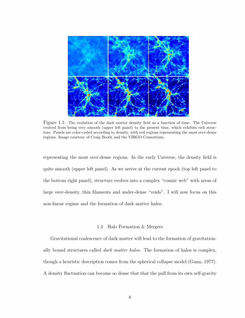
Figure 1.1: The evolution of the dark matter density field as a function of time. The Universeevolved from being very smooth (upper left panel) to the present time, which exhibits rich struc-ture. Panels are color-coded according to density, with red regions representing the most over-denseregions. Image courtesy of Craig Booth and the VIRGO Consortium.

representing the most over-dense regions. In the early Universe, the density field is

quite smooth (upper left panel). As we arrive at the current epoch (top left panel to

the bottom right panel), structure evolves into a complex “cosmic web” with areas of

large over-density, thin filaments and under-dense “voids”. I will now focus on this

non-linear regime and the formation of dark matter halos.

1.3 Halo Formation & Mergers

Gravitational coalescence of dark matter will lead to the formation of gravitation-

ally bound structures called dark matter halos. The formation of halos is complex,

though a heuristic description comes from the spherical collapse model (Gunn, 1977).

A density fluctuation can become so dense that that the pull from its own self-gravity

8

wins out over the expansion of the Universe. If we approximate this small fluctu-

ation as a sphere, then at a “turn around” point where the sphere has reached a

critical radius at which its own self-gravity dominates, then the density fluctuation

will collapse to form a dark matter halo. Ultimately, total collapse will never oc-

cur due to the fact that the kinetic energy associated with collapse is converted into

random particle motions. In this model, when the sphere will collapse to half its

critical radius, the halo will be in virial equilibrium - the kinetic energy K associated

with random motions of the dark matter particles is equal to half the gravitational

potential U of the particles (K = −12U). In essence, this means that virialization oc-

curs when the density contrast between the halo and the background density reaches

some critical value, ∆vir. The spherical collapse model predicts this to occur at

∆vir = 1 + δvir = ρρ∼= 200. ∆vir can be written more generally as a function of time,

∆vir(z) = Ω−1m × [18π2 + 82(Ωm − 1) − 39(Ωm − 1)2] (Bryan & Norman, 1998).

Unfortunately, halo formation is not as simple as the spherical collapse model.

In nature, halos do not always form in isolation, rather they can grow through the

accretion of smaller halos. Since halos are believed to be the natural sites for galaxies

to reside, knowing the merger history of halos is crucial for understanding how galaxies

evolve and assemble.

9

1.3.1 The Halo Mass Function

The Halo Mass Function describes the abundance of halos in the Universe and can

be approximated by an extension of the spherical collapse model. Press & Schechter

(1974) used simple Gaussian random field statistics to derive a halo mass function,

since the assumption is that halos form in the peaks in the Gaussian random density

field of dark matter. The number of halos per unit volume in the mass range M to

M + δM is ( dndM

) × δM , where,

dn

dM(M, t) =

(2

π

)1/2 ρ

M2

δc(t)

σ(M)

∣

∣

∣

d ln σ

d ln M

∣

∣

∣× exp

[

−δ2c (t)

2σ2(M)

]

. (1.7)

σ(M) is the variance of the density field (smoothed on a mass scale M = 4π3ρR3) and

δc(t) is the critical density for a halo to collapse at time t (Eke et al., 1996).

It is important to note that there is a characteristic mass scale, M∗(z), associated

with the halo mass function. M∗(z) is the typical mass scale (at a given redshift) for

a halo to collapse (M∗(z) ≈ 1012M⊙ today). The halo mass function has an intrinsic

shape where the number density of halos at the low-mass end is a decreasing power-

law function ( dndM

∝ M−α, α ≈ 1.8), because the initial power spectrum predicts

that small fluctuations are very abundant. Conversely, very large fluctuations are

rare, hence, large mass halos will be uncommon. As a result, the halo mass function

begins to turn over and exponentially drop off at masses greater than M∗(z). Though

this analytic formalism does not provide an extremely accurate description of results

from dark matter N-body simulations (e.g., Zentner, 2007; Robertson et al., 2009), it

10

is nonetheless a remarkably elegant and useful picture for halo formation.

1.3.2 Halo Structure

Halos are characterized by their large over-densities, which correspond, roughly,

to virialized regions of dark matter. Again, utilizing the spherical collapse model, we

can define a virial radius that is related to this density contrast (∆vir),

Rvir =( 3M

4πρ∆vir

)1/3

(1.8)

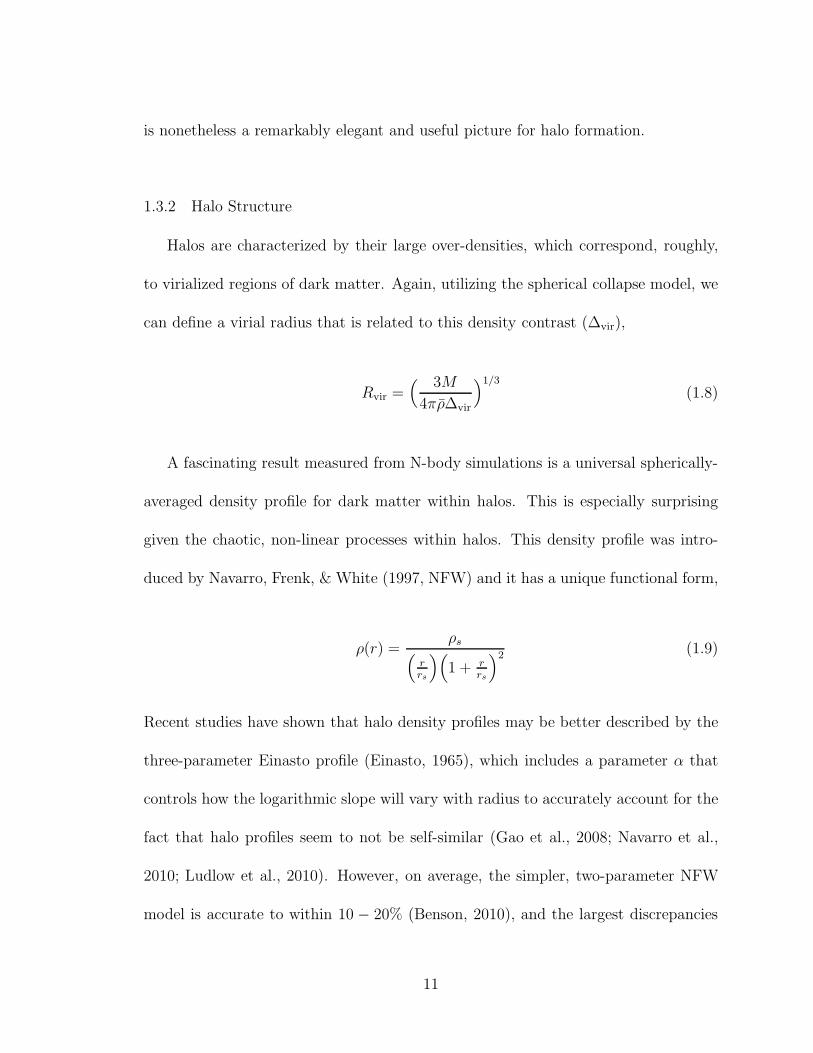
A fascinating result measured from N-body simulations is a universal spherically-

averaged density profile for dark matter within halos. This is especially surprising

given the chaotic, non-linear processes within halos. This density profile was intro-

duced by Navarro, Frenk, & White (1997, NFW) and it has a unique functional form,

ρ(r) =ρs

(

rrs

)(

1 + rrs

)2 (1.9)

Recent studies have shown that halo density profiles may be better described by the

three-parameter Einasto profile (Einasto, 1965), which includes a parameter α that

controls how the logarithmic slope will vary with radius to accurately account for the

fact that halo profiles seem to not be self-similar (Gao et al., 2008; Navarro et al.,

2010; Ludlow et al., 2010). However, on average, the simpler, two-parameter NFW

model is accurate to within 10 − 20% (Benson, 2010), and the largest discrepancies

11

arise very close to halo centers where baryonic physics are expected to affect the dark

matter profile. The NFW profile implies that at small radii the slope of the density

profile (in log space) decreases as r−1, transitions to r−2 at a characteristic scale

radius that weakly depends on halo mass, rs, then drops off as r−3 at large radii. The

ratio of the scale radius to a halo’s virial radius is defined through the concentration

parameter

C =rsRvir

(1.10)

which is a strong reflection of a halo’s assembly history (Wechsler et al., 2002), with

halos that formed earlier being more concentrated (Prada et al., 2011). It has also

been found that more massive halos are less concentrated (e.g., Bullock et al., 2001;

Maccio et al., 2008), though there is large scatter in this C−Mass relation.

1.4 Connecting the Dark and Light Sectors

Dark matter halos set the backdrop for the formation of the luminous structures

that we can observe. Knowing key ingredients of this dark sector, such as halo

formation and merging, the halo mass function, and the internal structure of halos, we

can take on the formidable problem of how galaxies are connected to these virialized

structures they reside in.

Galaxies are the “lighthouses” of the Universe, informing us about the overall

distribution of matter in the Universe. I now turn to an introduction to the complex

nature of how galaxies form and how we can use their spatial clustering to tackle

12

several unsolved problems relating to their formation and evolution, which constitutes

the crux of this work.

1.4.1 The Formation of Galaxies

Dark matter is ∼ 6× more prevalent than the ordinary baryonic that comprises

galaxies. Thus, it is plausible that the distribution of baryons may trace the underly-

ing dark matter density field. Shortly after recombination, as the primordial density

fluctuations began to collapse, so too did the pristine gas that resided in these regions

of over-density. The hot gas in halos cools and condenses as it sinks towards the po-

tential well minimum (White & Rees, 1978; Blumenthal et al., 1986). Therefore, the

density fluctuations that gravitationally attracted dark matter and gas seeded the

formation of halos and galaxies.

The first “proto-galaxies” consisted primarily of neutral hydrogen and, to a lesser

extent, helium. Unlike the formation of halos which is governed by the simple, colli-

sionless, dissipative nature of dark matter, the proto-galactic gas can collide and lose

energy, causing it to collapse. These collisions of clumps of gas induce shock fronts

of extremely high density and the heated gas will then sufficiently cool to become a

nursery for star formation. Continual collapse will cause the gas to settle into a ro-

tating disk. The galactic ecosystem involves the recycling of available gas due to the

life-cycle of stars. Older generations of stars will deposit gas back into the surround-

ing environment, enriching the intergalactic medium resulting in a new generation

13

of stars to be formed. However, this re-processing can not last forever and the gas

reservoir may be quenched. Additionally, energy feedback from supernovae or a mas-

sive central black hole (AGN) can blow out available gas, inhibiting star formation.

Hence, galaxies that formed very early may no longer exhibit signs of star formation

and are typically red (and elliptical in shape due to morphological disruptions as a

result of galaxy mergers) due to the dimming of the stellar populations, while more

recently forming galaxies are typically blue (and disk-shaped).

As discussed in § 1.3, dark matter halos can grow through the accretion of smaller

halos, and this process is naturally extended to galaxies. When a galaxy merges into

a larger halo it will experience intense gravitational processes. For example, the tidal

field of the larger halo can act to shred the galaxy apart. Also, dynamical friction

causes the merged galaxy to spiral towards the halo potential well minimum. Thus,

the larger, central galaxy can grow by cannibalizing smaller galaxies. These ideas

are expounded upon in detail in Chapters II and III. Ultimately, galaxy formation

is extremely complex and requires a complete understanding of gas/stellar dynamics

(collisional processes), star formation, and feedback mechanisms.

1.4.2 Subhalos & Galaxies

When a smaller halo merges into a larger one, it can retain its integrity as a self-

bound, orbiting dark matter entity. These accreted objects are dubbed “subhalos” or

“substructure” (Ghigna et al., 2000; Klypin et al., 1999a; Moore et al., 1999; Diemand

14

et al., 2004; Kravtsov et al., 2004a). When a halo is accreted by a larger halo, thus

becoming a subhalo, the galaxy within it becomes a “satellite” galaxy within a galaxy

group or cluster. Understanding the detailed relationship between (satellite) galaxies

and (sub) halos is a long-standing focus of galaxy formation theory.

In the hierarchical paradigm, these smaller objects, upon merging, become victims

of intense tidal fields within their “parent” or “host” halo. The dark matter mass

associated with a subhalo may be rapidly stripped upon infall. But what happens to

the galaxy residing in the subhalo? Does it change color and/or morphology? How is

the gas component affected? How is star formation altered? Do some, none, or all of

the stars associated with the galaxy become unbound as well? These are challenging

questions to answer and predominantly remain unresolved. In this thesis I look to

shed light on this final question of satellite galaxy stellar mass loss.

Tidal stripping acts on the periphery of the subhalo first, causing dark matter

mass loss. This suggests that the luminous galaxy, residing deep in the potential

well of the subhalo, may be unharmed. However, after enough time has elapsed,

stripping of stars may begin to occur as well. Massive halos are known to have

unbound, diffuse stellar material unassociated with any particular satellite galaxy (or

the central galaxy) of the system. These liberated stars that are ripped from satellite

galaxies are the likely source of “intrahalo light” (IHL: e.g., Gallagher & Ostriker,

1972; Mihos et al., 2005; Gonzalez et al., 2007). In Chapter III, I constrain the

liberation of stars from satellite galaxies by connecting stellar mass loss to subhalo

15

dark matter mass loss using galaxy clustering (which I describe in detail in § 1.4.3)

and IHL observations (this work has been submitted for publication in Watson et al.

2011c).

1.4.3 Spatial Clustering

The principal strategy of this work is to use the spatial clustering of galaxies to

gain insight into fundamental aspects of galaxy formation. To quantify the degree

of clustering, we consider two infinitesimally small spheres centered on two objects,

located at −→r1 and −→r2 in space. If the spheres have volume V1 and V2 respectively, then

the joint probability of finding these two objects at a separation −→r = −→r1 −−→r2 is,

dP12 = n2[1 + ξ(−→r )]dV1dV2 (1.11)

where n is the mean number density of objects in space, and ξ(−→r ) is the two-point

correlation function. The two-point correlation function is the excess probability of

finding a pair of objects at a given separation −→r relative to a random distribution. The

full series of n-point correlation functions will completely describe the distribution of

large-scale structure. However, due to observational limitations, most work exploits

the two-point correlation function (which I will just refer to as the correlation function

throughout the remainder of the Introduction), though powerful new galaxy surveys

(see § 1.4.4) have now made it possible to measure higher moments, such as the the

three-point correlation function (McBride et al., 2011).

16

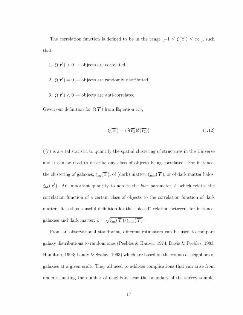
The correlation function is defined to be in the range [−1 ≤ ξ(−→r ) ≤ ∞ ], such

that,

1. ξ(−→r ) > 0 → objects are correlated

2. ξ(−→r ) = 0 → objects are randomly distributed

3. ξ(−→r ) < 0 → objects are anti-correlated

Given our definition for δ(−→r ) from Equation 1.5,

ξ(−→r ) = 〈δ(−→r1)δ(−→r2)〉 (1.12)

ξ(r) is a vital statistic to quantify the spatial clustering of structures in the Universe

and it can be used to describe any class of objects being correlated. For instance,

the clustering of galaxies, ξgg(−→r ), of (dark) matter, ξmm(−→r ), or of dark matter halos,

ξhh(−→r ). An important quantity to note is the bias parameter, b, which relates the

correlation function of a certain class of objects to the correlation function of dark

matter. It is thus a useful definition for the “biased” relation between, for instance,

galaxies and dark matter: b =√

ξgg(−→r )/ξmm(−→r ) .

From an observational standpoint, different estimators can be used to compare

galaxy distributions to random ones (Peebles & Hauser, 1974; Davis & Peebles, 1983;

Hamilton, 1993; Landy & Szalay, 1993) which are based on the counts of neighbors of

galaxies at a given scale. They all need to address complications that can arise from

underestimating the number of neighbors near the boundary of the survey sample.

17

Figure 1.2: The galaxy two-point correlation function of luminous red galaxies (LRGs) from theSloan Digital Sky Survey. An ∼ r−2 power-law slope spans roughly four orders of magnitude inLRG-LRG separation scales. Image (modified) from Masjedi et al. (2006).

One of the more common estimators is from Landy-Szalay (Landy & Szalay, 1993),

ξ =DD − 2DR +RR

RR(1.13)

where DD, DR and RR are the normalized numbers of weighted data-data, data-

random and random-random pairs in each bin of radial separation. Figure 1.2 is

the measured correlation function of luminous red galaxies (massive, bright elliptical

galaxies) from the Sloan Digital Sky Survey (see § 1.4.4). Nature has provided a

rather simple approximate power-law form for galaxies, ξgg(−→r ) = (

−→r

−→r 0

)−γ, where −→r 0

(an intrinsic correlation length that depends on the objects being correlated) and

γ (the slope of the power-law) are fit to a given galaxy sample. Here, γ = 2 over

an enormous range of scales spanning ∼ 4 orders of magnitude. The ξ(r) ∝ r−2

18

power-law form has been known for over four decades, though the physical processes

governing this simple shape was an unsolved problem. As a result of the explosion of

high quality data over the last decade mapping the spatial distribution of galaxies,

I confront this long-standing conundrum from a theoretical standpoint in Chapter II

with the aim of revealing the physics behind the power-law nature of ξgg(−→r ) (the

results of which have been published in Watson et al. 2011b).

1.4.4 Galaxy Surveys

The Center for Astrophysics Redshift Surveys (CfA: Davis et al. 1982, CfA2:

Huchra et al. 1983) were the first surveys to attempt to map the 3-dimensional large-

scale structure of the Universe. The aim was to measure the radial velocities of a

large sample of galaxies in the northern sky. CfA provided us with the first ever

mapping of the local Universe, as well as the first measurements of galaxy clustering

properties. CfA2 was started several years later, and measured the redshifts to nearly

18,000 galaxies. These surveys clearly demonstrated that the galaxy distribution is

far from random. Galaxies were seen to be highly clustered and surrounded by voids.

The Two Degree Field Galaxy Redshift Survey (2dFGRS: Colless et al. 2001)

drastically extended the number of galaxies observed by probing a significantly larger

volume. 2dFGRS used a 4-meter telescope with a two degree field of view, mapping

∼ 2, 000 square degrees. They retrieved spectra of ∼ 250, 000 galaxies. This allowed

for a high precision determination of the large-scale galaxy distribution in the local

19

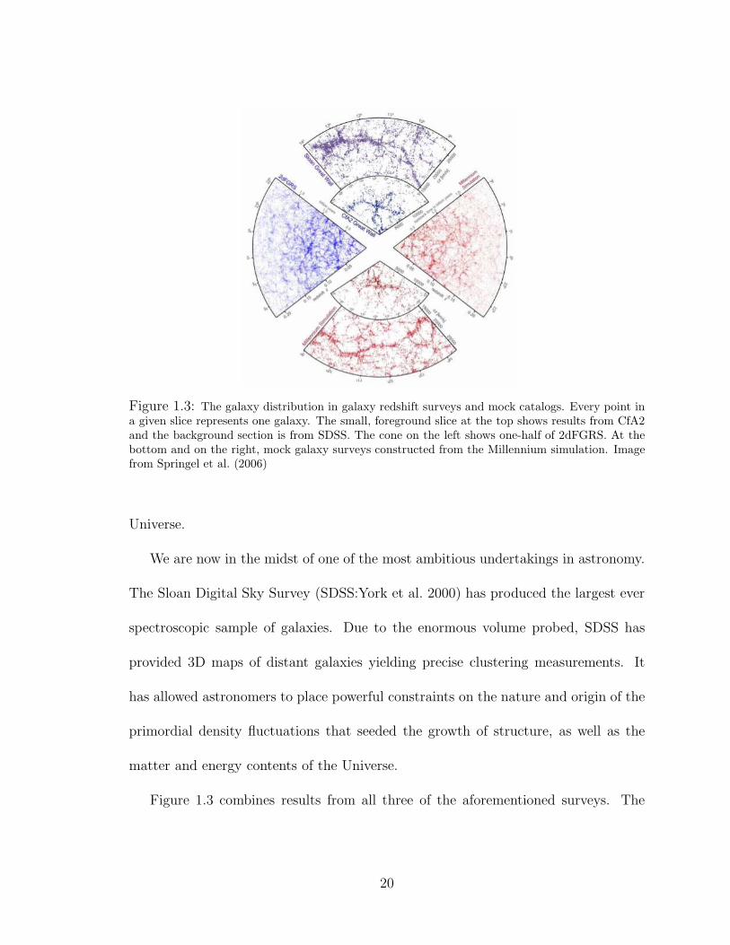
Figure 1.3: The galaxy distribution in galaxy redshift surveys and mock catalogs. Every point ina given slice represents one galaxy. The small, foreground slice at the top shows results from CfA2and the background section is from SDSS. The cone on the left shows one-half of 2dFGRS. At thebottom and on the right, mock galaxy surveys constructed from the Millennium simulation. Imagefrom Springel et al. (2006)

Universe.

We are now in the midst of one of the most ambitious undertakings in astronomy.

The Sloan Digital Sky Survey (SDSS:York et al. 2000) has produced the largest ever

spectroscopic sample of galaxies. Due to the enormous volume probed, SDSS has

provided 3D maps of distant galaxies yielding precise clustering measurements. It

has allowed astronomers to place powerful constraints on the nature and origin of the

primordial density fluctuations that seeded the growth of structure, as well as the

matter and energy contents of the Universe.

Figure 1.3 combines results from all three of the aforementioned surveys. The

20

upper two slices show results from SDSS and CFA2 and the left slice is from 2dFGRS

(each point represents a galaxy). At the bottom and on the right are mock galaxy

surveys constructed using semi-analytic techniques to model the distribution of galax-

ies within the dark matter distribution in the Millennium simulation (Springel et al.,

2005). Rich structure is evident with highly clustered regions of galaxies surrounded

by large under-dense voids.

1.4.5 Redshift Space Distortions

Distance measures are a common thorn in the side of astronomers. Simply having

spectroscopic redshifts of galaxies will not give a true 3-dimensional picture. This is

because an important signature of gravitational instability is that collapsing struc-

tures will generate peculiar velocities. By definition, redshift compares the observed

wavelength to the intrinsic wavelength. How the observed wavelength is shifted can

arise from two separate effects when considering cosmological scales. First, there is

the redshift associated with objects moving with the Hubble flow (as discussed in

§ 1.1). Second, there is the redshift contribution due to the intrinsic line-of-sight

motions of the objects observed (the doppler effect),

zdoppler ≃−→v pec

c(1.14)

where −→v pec is the peculiar (line-of-sight) velocity relative to the Hubble flow (c is the

speed of light). Therefore, redshift as defined for large-scale structure is the product

21

of the cosmological and doppler contributions,

1 + z = (1 + zcosmo)(1 + zdoppler) (1.15)

A measured redshift combines Hubble’s law with the radial component of −→v pec, such

that cz ≃ H0r + −→v pec. If structure forms via gravitational collapse, there should be

coherent infall velocities on large scales where −→v pec can be small compared to the

size of the associated structure. In other words, consider an enormous supercluster

(like the “Sloan Great Wall” Gott et al. 2005) of size R0. If R0 × H > −→v pec then

there is an observed squashing or flattening of structure in redshift-space, known

as the “Kaiser Effect” (Kaiser, 1987). Conversely, in the case of a galaxy cluster,

peculiar velocities associated with the random orbital motions of galaxies are much

larger than R0×H . This produces what is known as the “finger-of-God” effect, where

structures appear highly elongated in redshift space. Since galaxy redshift is not a

“true” distance, we decompose the separation r between galaxies into perpendicular,

rp, and parallel, line-of-sight, π, components to encapsulate these redshift distortions.

Perpendicular separations are true measures of distance, but the radial separations

are distorted by −→v pec. In Figure 1.4, both effects can be clearly seen in the 2-

dimensional correlation function, ξ(rp, π), as measured in the 2dFGRS (Peacock et al.,

2001). Here, rp is denoted as σ and the upper-right quadrant has been mirrored

along both axes to illustrate deviations from circular symmetry. In the absence of

redshift space distortions, the contours would be isotropic. However, for small-scale

22

Figure 1.4: The 2-dimensional correlation function as measured in the 2dF Galaxy Redshift Survey(Peacock et al., 2001). The separation r between galaxies is decomposed into perpendicular, rp, andparallel, π, components. Coherent infall velocities on large scales where peculiar velocities canbe small compared to an associated large structure (such as the “Sloan Great Wall”) produce anobserved “flattening” of structure. Conversely, for smaller regions such as galaxy clusters, peculiarvelocities associated with the random orbital motions of galaxies are much larger than the clusterthey reside in resulting in structures appearing highly elongated in redshift space (flattening andelongation are highlighted by the red arrows). The upper-right quadrant has been mirrored alongboth axes to highlight deviations from circular symmetry. In the absence of redshift space distortions,the contours would be isotropic.

projected separations, the contours are elongated from the finger-of-God effect, while

compression from the Kaiser effect is evident on large scales (as highlighted by the

red arrows).

To compensate for redshift distortions it is common practice to compute the pro-

jected correlation function, wp(rp), by integrating along the line of sight (Davis &

Peebles, 1983; Zehavi et al., 2004):

wp(rp) = 2

∫

∞

0

ξ(rp, π)dπ. (1.16)

For a typical galaxy sample, the line-of-sight component is integrated to πmax ∼

23

50h−1Mpc to incorporate most correlated pairs (e.g., Zehavi et al., 2011).

1.4.6 Dark Matter & Galaxies on Extremely Small Scales

This thesis revolves strongly around modeling of observational measurements of

the projected correlation function of galaxies. The galaxy correlation function on

scales smaller than the virial radii of the largest dark matter halos (r . 1Mpc)

is dictated by the radial distribution of galaxies. Therefore, the measured galaxy

correlation function itself is a powerful tool for shedding light on how galaxies trace

the underlying dark matter within halos since the radial distribution of dark matter

is fairly well pinned down. Chapters II and III involved modeling of the correlation

function on scales ∼ 100kpc − 20Mpc to glean information on galaxy formation

and evolution. But what about on scales much deeper within individual halos, r <

100kpc?

Galaxies, being massive and extended, are subject to dynamical mechanisms such

as dynamical friction and mass loss. These processes become more chaotic towards the

centers of halos where the tidal field is strongest, and should affect large and massive

(and hence, very luminous) objects more than small ones. Therefore, the very small-

scale correlation function can be used to investigate the luminosity dependence of

the radial distribution of satellite galaxies and the degree to which it differs from an

NFW distribution. I take advantage of recent precision measurements of projected

correlation functions from SDSS to perform such a study and this is addressed in

24

Chapters IV and V (the results have been published in Watson et al. 2010, 2011a).

25

Chapter II

THE GALAXY CORRELATION FUNCTION CONSPIRACY

Abstract

We model the evolution of galaxy clustering through cosmic time to investigate the

nature of the power-law shape of ξ(r), the galaxy two-point correlation function.

While ξ(r) on large scales is set by primordial fluctuations, departures from a power

law are governed by galaxy pair counts on small scales, subject to non-linear dynamics.

We assume that galaxies reside within dark matter halos and subhalos. Therefore,

the shape of the correlation function on small scales depends on the amount of halo

substructure. We use a semi-analytic substructure evolution model to study subhalo

populations within host halos. We find that tidal mass loss and, to a lesser extent,

dynamical friction dramatically deplete the number of subhalos within larger host

halos over time, resulting in a ∼ 90% reduction by z = 0 compared to the number of

distinct mergers that occur during the assembly of a host halo. We show that these

non-linear processes resulting in this depletion are essential for achieving a power-law

ξ(r). We investigate how the shape of ξ(r) depends on subhalo mass (or luminosity)

and redshift. We find that ξ(r) breaks from a power law at high masses, implying that

only galaxies of luminosities . L∗ should exhibit power-law clustering. Moreover, we

demonstrate that ξ(r) evolves from being far from a power law at high redshift, toward

26

a near power-law shape at z = 0. We argue that ξ(r) will once again evolve away from

a power law in the future. This is in large part caused by the evolving competition

between the accretion and destruction rates of subhalos over time, which happen to

strike just the right balance at z ≈ 0. We then investigate the conditions required

for ξ(r) to be a power law in a general context. We use the halo model along with

simple parametrizations of the halo occupation distribution (HOD) to probe galaxy

occupation at various masses and redshifts. We show that key ingredients determining

the shape of ξ(r) are the fraction of galaxies that are satellites, the relative difference

in mass between the halos of isolated galaxies and halos that contain a single satellite

on average, and the rareness of halos that host galaxies. These pieces are intertwined

and we find no simple, universal rule for which a power-law ξ(r) will occur. However,

we do show that the physics responsible for setting the galaxy content of halos do not

care about the conditions needed to achieve a power law ξ(r) and these conditions are

met only in a narrow mass and redshift range. We conclude that the power-law nature

of ξ(r) for L∗ and fainter galaxy samples at low redshift is a cosmic coincidence.

2.1 Introduction

The two-point correlation function of galaxies was measured four decades ago

and found to be consistent with a ξ(r) ∝ r−2 power law (Totsuji & Kihara, 1969;

Peebles, 1973; Hauser & Peebles, 1973; Peebles & Hauser, 1974; Peebles, 1974). Since

that time, successively larger galaxy redshift surveys (e.g., Huchra et al., 1983; da

27

Costa et al., 1988; Santiago et al., 1995; Shectman et al., 1996; Saunders et al., 2000;

Colless et al., 2001; York et al., 2000) have mapped the distribution of galaxies with

ever increasing precision and confirmed correlation functions consistent with power

laws over a large range of scales (e.g., de Lapparent et al., 1988; Marzke et al., 1995;

Hermit et al., 1996; Tucker et al., 1997; Jing et al., 1998, 2002; Norberg et al., 2002;

Zehavi et al., 2002). The scales on which a single power-law description is valid span a

range from large regions exhibiting mild density fluctuations (r & 10 Mpc), to smaller

regions with large density fluctuations experiencing rapid non-linear evolution (r ∼

1−10 Mpc), to collapsed and virialized galaxy groups and clusters (r . 1 Mpc). It has

long been noted that the lack of any feature delineating the transitions among these

scales is surprising (e.g., Peebles, 1974; Gott & Turner, 1979; Hamilton & Tegmark,

2002; Masjedi et al., 2006; Li & White, 2010). This is especially true given that

the matter correlation function in the now well-established concordance cosmological

model differs significantly from a power law. In this paper, we return to this long-

standing problem and address the origin of a power-law galaxy correlation function

in the context of our modern paradigm for the growth of cosmic structure.

This conundrum can be refined within the contemporary framework in which

galaxies live within virialized halos of dark matter (White & Rees, 1978; Blumenthal

et al., 1984). In such a model, galaxy clustering statistics can be modeled as a

combination of dark matter halo properties and a halo occupation distribution (HOD)

that specifies how galaxies occupy their host halos (e.g., Peacock & Smith, 2000;

28

Scoccimarro et al., 2001; Berlind & Weinberg, 2002; Cooray & Sheth, 2002). In this

halo model approach, the galaxy correlation function is a sum of two terms: On small

scales, pairs of galaxies reside in the same host dark matter halo (the “one-halo”

term), whereas on large scales, the individual galaxies of a pair reside in distinct

halos (the “two-halo” term). These two terms depend on the HOD in different ways,

requiring delicate tuning in order to spawn an unbroken power law (e.g., Berlind &

Weinberg, 2002). Consequently, a feature in ξ(r) at scales corresponding to the radii

of the typical, virialized halos that host luminous galaxies is expected.

In a dramatic success for the halo model, Zehavi et al. (2004) first detected a

statistically-significant departure from a power law due to the high precision mea-

surements of the Sloan Digital Sky Survey, and demonstrated that the halo model

provides an acceptable fit to the data. Zehavi et al. (2005b) confirmed this result,

adding that power-law departures grow stronger with galaxy luminosity (see also

Blake et al., 2008; Ross et al., 2010). ξ(r) has since been shown to deviate from a

power law at high redshifts (Ouchi et al., 2005; Lee et al., 2006; Coil et al., 2006;

Wake et al., 2011). Nevertheless, it remains a fact that deviations from a power law

at low redshifts are small and the galaxy correlation function is roughly a power law

over an enormous range of galaxy-galaxy separations. Deviations have been revealed

only through ambitious observational efforts.

Halos are known to be replete with self-bound structures, dubbed “subhalos”

(Ghigna et al., 1998; Klypin et al., 1999b; Moore et al., 1999), and both halos and

29

subhalos are thought to be the natural sites of galaxy formation. Subhalos were

isolated halos in their own right, hosting distinct galaxies before merging into a larger

group or cluster halo1. Remarkably, the clustering of host halos along with their

associated subhalos is very similar to that of observed galaxies (Kravtsov & Klypin,

1999; Colın et al., 1999; Kravtsov et al., 2004a), suggesting a simple correspondence

of galaxies with host halos and subhalos. This was clearly demonstrated by Conroy

et al. (2006) who compared the correlation functions of hosts and subhalos to that of

galaxies over a broad range of luminosities and redshifts (z ∼ 0−4), finding excellent

agreement. These results indicate that an understanding of the physics governing the

subhalo populations within host halos may provide insight into the physics of galaxy

clustering and the near power-law form of the galaxy two-point correlation function.

In this paper, we examine the causes of the observed power-law correlation func-

tion by studying the mergers, survival, and/or destruction of dark matter subhalos.

Our focus in this paper is on the gross features of the galaxy two-point function

and not on detailed comparisons to specific data sets. We explore more sophisti-

cated galaxy-halo assignments and statistical comparisons with data in a forthcoming

follow-up study (Watson et al. in prep.).

We argue that the nearly power-law, low-redshift galaxy correlation function is

a coincidence. The correlation function of common L . L∗ galaxies evolves from

1Satellites or subhalos are used throughout the paper to refer to self-bound entities lying withinthe virial radius of a larger halo. Those that do not lie within a larger system are designated ascentrals, host halos or simply hosts.

30

relatively strong small-scale clustering at early times, through a power-law at the

present epoch, and most likely toward relatively weak small-scale clustering in the fu-

ture. The origin of the present-day power law, in turn, relies on the tuning of several

disconnected ingredients, at least three of which are: the normalization of primordial

density fluctuations determined by early Universe physics; a halo mass scale for effi-

cient galaxy formation determined largely by atomic physics, stellar physics, and the

physics of compact objects; and relative abundances of baryonic matter, dark matter,

and dark energy in the Universe.

Our paper is organized as follows. In § 2.2 we review the halo model and restate

the problem in terms of this framework. In § 2.3 we give an overview of our primary

modeling technique. In § 2.4 we investigate the individual roles of merging, dynamical

friction, and mass loss in shaping the halo occupation statistics of subhalos, as well

as the resulting halo correlation function. In § 2.5 we show how ξ(r) depends on

host halo mass and redshift. In § 2.6 we explore a standard parametrization of the

HOD to see what is required to get a power-law ξ(r), and we predict the masses and

redshifts at which a power-law ξ(r) can be constructed. In § 2.7 we give a summary of

our results and our primary conclusions. Throughout this paper, we work within the

standard, vacuum-dominated, cold dark matter (ΛCDM) cosmological model with

Ωm = 0.3, ΩΛ = 0.7, Ωb = 0.04, h0 = 0.7, σ8 = 0.9, and ns = 1.0. These values

differ slightly form the WMAP best-fit values, however this has little effect on our

general results and was chosen in order to compare to previous work that used similar

31

cosmological models.

2.2 A Modern Restatement of the Problem in Halo Model Language

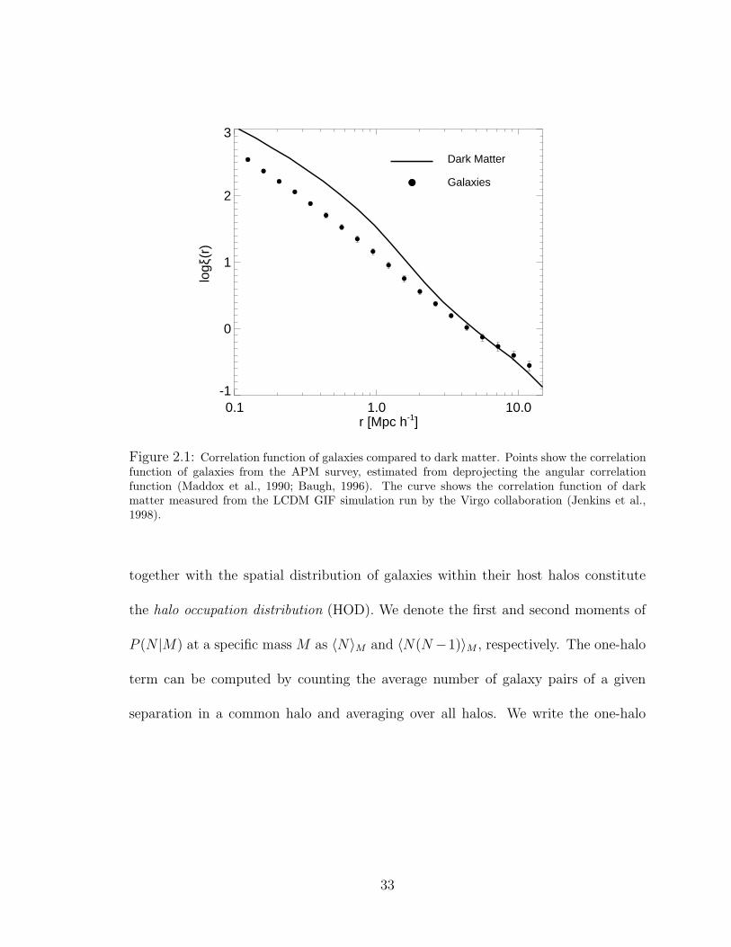
Though the observed galaxy correlation function is nearly a power law, the matter

correlation function predicted by the concordance cosmological model is not. This is

evident in Figure 2.1. On scales corresponding to collapsed objects, the dark matter

correlation function exceeds the values that would be obtained by extrapolating the

larger-scale power law to small scales. However, galaxies are biased with respect

to dark matter in such a way as to counteract this excess. We can examine this

discrepancy in terms of the halo model. If the reader is familiar with the halo model

formalism, he or she may wish to skip to § 2.2.2

2.2.1 Halo Model Basics

Assuming that all galaxies live within virialized dark matter halos, the galaxies

comprising any pair can come either from within the same halo (the one-halo term) or

from two separate halos (the two-halo term). The correlation function is then given

as the sum of these two terms

ξ(r) = ξ(r)1halo + ξ(r)2halo + 1, (2.1)

(e.g., Cooray & Sheth 2002; for this particular form of the equation see Zheng 2004).

The probability distribution P (N |M) that a halo of mass M contains N galaxies

32

0.1 1.0 10.0r [Mpc h-1]

-1

0

1

2

3

log ξ

(r)

Dark Matter

Galaxies

Figure 2.1: Correlation function of galaxies compared to dark matter. Points show the correlationfunction of galaxies from the APM survey, estimated from deprojecting the angular correlationfunction (Maddox et al., 1990; Baugh, 1996). The curve shows the correlation function of darkmatter measured from the LCDM GIF simulation run by the Virgo collaboration (Jenkins et al.,1998).

together with the spatial distribution of galaxies within their host halos constitute

the halo occupation distribution (HOD). We denote the first and second moments of

P (N |M) at a specific mass M as 〈N〉M and 〈N(N−1)〉M , respectively. The one-halo

term can be computed by counting the average number of galaxy pairs of a given

separation in a common halo and averaging over all halos. We write the one-halo

33

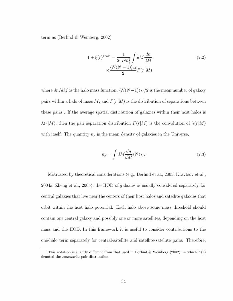
term as (Berlind & Weinberg, 2002)

1 + ξ(r)1halo =1

2πr2n2g

∫

dMdn

dM(2.2)

×〈N(N − 1)〉M

2F (r|M)

where dn/dM is the halo mass function, 〈N(N−1)〉M/2 is the mean number of galaxy

pairs within a halo of mass M , and F (r|M) is the distribution of separations between

these pairs1. If the average spatial distribution of galaxies within their host halos is

λ(r|M), then the pair separation distribution F (r|M) is the convolution of λ(r|M)

with itself. The quantity ng is the mean density of galaxies in the Universe,

ng =

∫

dMdn

dM〈N〉M . (2.3)

Motivated by theoretical considerations (e.g., Berlind et al., 2003; Kravtsov et al.,

2004a; Zheng et al., 2005), the HOD of galaxies is usually considered separately for

central galaxies that live near the centers of their host halos and satellite galaxies that

orbit within the host halo potential. Each halo above some mass threshold should

contain one central galaxy and possibly one or more satellites, depending on the host

mass and the HOD. In this framework it is useful to consider contributions to the

one-halo term separately for central-satellite and satellite-satellite pairs. Therefore,

1This notation is slightly different from that used in Berlind & Weinberg (2002), in which F (r)denoted the cumulative pair distribution.

34

we rewrite the one-halo term as (Berlind & Weinberg, 2002)

1 + ξ(r)1halo =1

2πr2n2g

∫

dMdn

dM(2.4)

×[

〈NcenNsat〉MFcs(r|M) +〈Nsat(Nsat − 1)〉M

2Fss(r|M)

]

,

where 〈NcenNsat〉M and 〈Nsat(Nsat − 1)〉M/2 are the mean number of central-satellite

and satellite-satellite pairs in hosts of massM , and Fcs(r|M) and Fss(r|M) are the pair

separation distributions of central-satellite and satellite-satellite pairs, respectively.

If the central galaxies always reside very close to the center of the host halo and

the average distribution of satellite positions within the host halo is λs(r|M), then

Fcs = λs(r|M) and Fss(r|M) is the convolution of λs(r|M) with itself. In practical

cases there is at most one central galaxy and satellites are only present in halos with

a central, so that 〈NcenNsat〉M = 〈Nsat〉M . The total fraction of galaxies that are

satellites in a sample is then

fsat = n−1g

∫

dMdn

dM〈Nsat〉M

=

∫

dM dndM

〈Nsat〉M∫

dM dndM

(〈Ncen〉M + 〈Nsat〉M). (2.5)

The satellite fraction, fsat, will prove an important quantity in determining the shape

of the galaxy correlation function.

On scales significantly larger than individual halos, the two-halo term dominates

the clustering strength. It is most simply written in Fourier space as (Cooray & Sheth

35

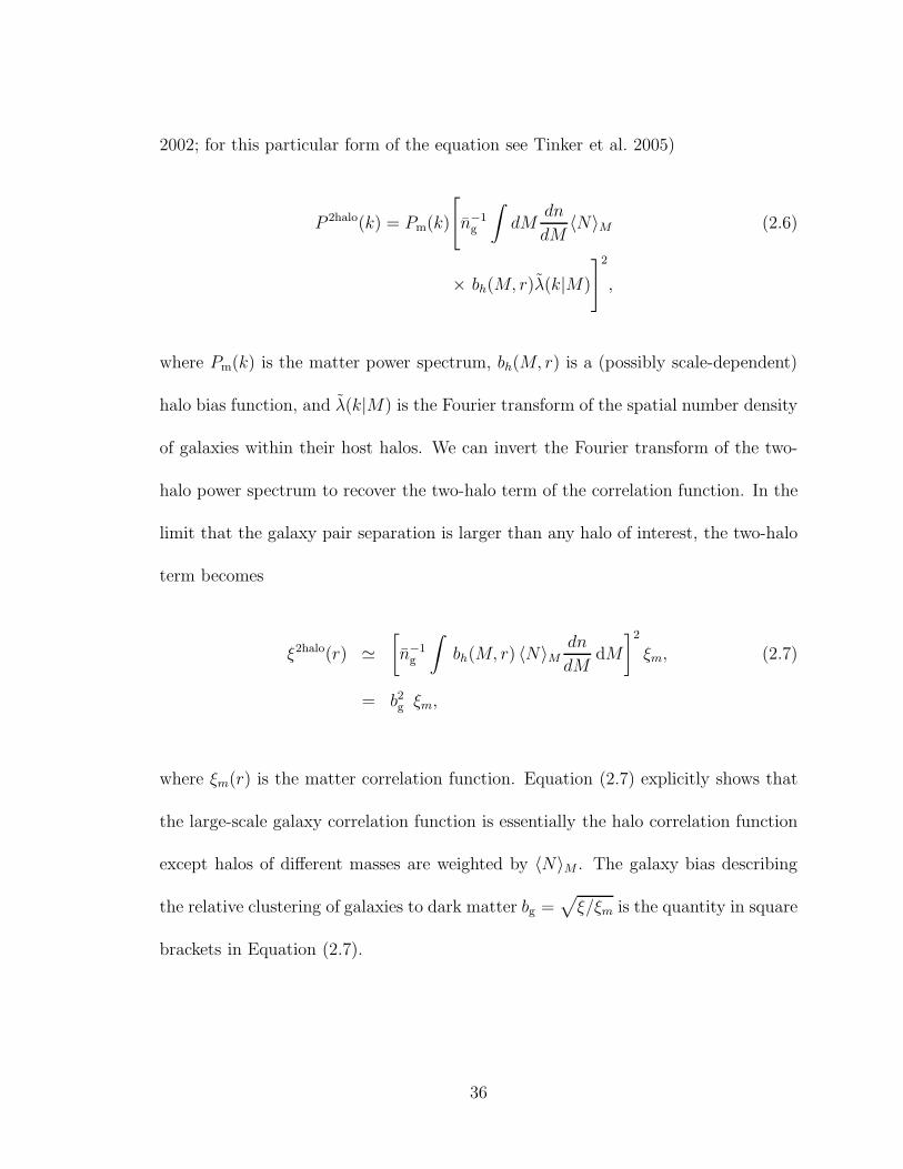
2002; for this particular form of the equation see Tinker et al. 2005)

P 2halo(k) = Pm(k)

[

n−1g

∫

dMdn

dM〈N〉M (2.6)

× bh(M, r)λ(k|M)

]2

,

where Pm(k) is the matter power spectrum, bh(M, r) is a (possibly scale-dependent)

halo bias function, and λ(k|M) is the Fourier transform of the spatial number density

of galaxies within their host halos. We can invert the Fourier transform of the two-

halo power spectrum to recover the two-halo term of the correlation function. In the

limit that the galaxy pair separation is larger than any halo of interest, the two-halo

term becomes

ξ2halo(r) ≃

[

n−1g

∫

bh(M, r) 〈N〉Mdn

dMdM

]2

ξm, (2.7)

= b2g ξm,

where ξm(r) is the matter correlation function. Equation (2.7) explicitly shows that

the large-scale galaxy correlation function is essentially the halo correlation function

except halos of different masses are weighted by 〈N〉M . The galaxy bias describing

the relative clustering of galaxies to dark matter bg =√

ξ/ξm is the quantity in square

brackets in Equation (2.7).

36

2.2.2 The Battle of the 1- Halo and 2- Halo Terms

Berlind & Weinberg (2002) showed that maintaining a power-law correlation func-

tion requires a careful balance between the one-halo and two-halo terms and is thus

quite difficult to achieve. This is because the one-halo term generally changes by a

larger amount than the two-halo term in response to changes to the HOD. A close

examination of Equations (2.3), (2.4), (2.6) and (2.7) reveals why this is the case.

Consider first the two-halo term as it is the simplest. On large scales, the two-halo

term is just a weighted average of the clustering of host halos. For simplicity, assume

(albeit incorrectly) the halo bias to be a constant function of halo mass. Increasing

〈N〉M increases both the number of two-halo pairs at a given separation (the square

of the integral in Eqs. [2.6] and [2.7]) and the number of random pairs n2g/2, by the

same amount. The reason the two-halo term is at all sensitive to the HOD is that the

bias of halos does depend on mass and so changing the relative number of galaxies

in high-mass vs. low-mass halos changes the weight in the average of the halo bias

in Equation (2.7). For example, assigning a large number of satellite galaxies to

high-mass halos increases ξ2halo(r) by weighting highly-biased, high-mass halos more

heavily. The possible range in the amplitude of the two-halo term is limited by the

variation of the halo bias function bh(M), within the mass range relevant to galaxies,

1011 . M/M⊙ . 1015. At low masses, the halo bias is bh ∼ 0.65 while, in the cluster

regime (M ∼ 1014h−1M⊙), it grows to values of bh ∼ 2 (Tinker et al., 2005). Bias

continues to grow with mass, but more massive halos are rare and do not contribute

37

much to the weighted average because dn/dM is minuscule. The two-halo term scales

like the square of the average bias bg in Equation (2.7), so the possible dynamic range

ξ2halo can display is, at most, a factor of ∼ 9 and is usually significantly smaller.

Simply put, the two-halo term depends weakly on the HOD because on large scales

it is not possible to make galaxies significantly more or less clustered than the host

halos they occupy.

On small scales, the one-halo term dominates and the situation is different. The

number of galaxy pairs within an individual halo scales with 〈N(N − 1)〉M while

the number of random pairs scales with n2g, or 〈N〉2M . It is instructive to break the

HOD into central and satellite galaxies. In the regime where there is one central

galaxy per halo, the mean number of central-satellite pairs is 〈NcenNsat〉M = 〈Nsat〉M ,

whereas the mean number of satellite-satellite pairs is 〈Nsat(Nsat−1)〉M/2. Assuming

a Poisson distribution for the number of satellite galaxies (Kravtsov et al., 2004a),

〈Nsat(Nsat − 1)〉M = 〈Nsat〉2M . The mean number of random pairs scales like (1 +

〈Nsat〉)2M . In the limit 〈Nsat〉M ≫ 1, the number of satellite-satellite pairs dominates

the number of central-satellite pairs, but in this limit both the number of one-halo

pairs and the square of the mean galaxy number density scale as 〈Nsat〉2M so the one-

halo term saturates to a maximum value and is insensitive to the number of satellite

galaxies per halo.

In most practical cases, the fraction of satellite galaxies in an observational sam-

ple is fsat . 0.25, so samples tend to be dominated by halos with satellite galaxy

38

populations in the opposite limit, 〈Nsat〉M ≪ 1. This is due to the fact that very

massive host halos are rare, so halos with 〈Nsat〉M > 1 are rare. With 〈Nsat〉M ≪ 1,

the central-satellite term dominates and the number of such pairs scales as 〈Nsat〉M

while the mean number density ng is approximately constant. Examination of Equa-

tions (2.4) and (2.5) reveals that in this regime ξ1halo scales in proportion to the

fraction of satellite galaxies and in inverse proportion to the number of host halos.

Host halo mass is largely fixed by requiring the galaxies in any sample to have an

appropriate average number density (this is why rare galaxies exhibit strong small-

scale clustering). Therefore, the one-halo term describing any given sample varies

approximately linearly with 〈Nsat〉M until 〈Nsat〉 > 1, at which point it saturates. It

is interesting that nearly all the sensitivity of the correlation function to the HOD

comes from central-satellite galaxy pairs in host halos where satellite galaxies are

uncommon!

In this work, we aim to understand the origin of the nearly power-law galaxy

correlation function. The relevant question is why is it that the number of galaxies

(or satellite galaxies to be more specific) per halo is set just so that the one-halo and

two-halo terms in the galaxy correlation function match smoothly, leaving only small

deviations from a single power law over several orders of magnitude in scale? We con-

front this problem by studying the properties and evolution of subhalo populations.

We now turn to some of the details of our modeling methods.

39

2.3 Overview of Halo Substructure Modeling

Our approach is to study the evolution of subhalos within virialized host halos

as a method to understand satellite galaxies and, in turn, the evolution of galaxy

clustering. We focus our attention on the relative strengths of small-scale and large-

scale clustering. We study subhalo populations using the approximate semi-analytic

model of Zentner et al. (2005, hereafter Z05). In this section, we briefly review the

fundamental aspects of the model that are of immediate relevance and we refer the

reader to Z05 for details and validation. The subhalo model is based on Zentner &

Bullock (2003) and is similar to the independent models of Taylor & Babul (2004,

2005a,b) and Penarrubia & Benson (2005), while sharing many features with other

approximate treatments of halo substructure (Oguri & Lee, 2004; van den Bosch et al.,

2005; Faltenbacher & Mathews, 2005; Purcell et al., 2007; Giocoli et al., 2008, 2009).

Semi-analytic models are an approximation to the calculations of large N -body

simulations, yet such models offer many advantages: (1) semi-analytic calculations are

computationally inexpensive; (2) they have no inherent resolution limits; (3) they en-

able the statistical study of subhalos within very large numbers of host halos; (4) they

allow the growth and mass-loss histories of particular subhalos to be tracked without

significant post-processing and analysis; (5) they make studies of model parame-

ter space tractable; and (6) semi-analytic models facilitate parsing complex physical

phenomena so that the relative importance of different physical effects may be un-

derstood. Our goal is to quantify the relative importance of merging, which increases

40

subhalo abundances, and dynamical friction and mass loss, which decrease subhalo

abundances. We also aim to explore predictions for subhalo populations and galaxy

correlation functions from high redshift to several Hubble times in the future. Z05

extensively tested the model we use in this paper and showed that the model produces

subhalo mass functions, occupation statistics, and radial distributions within hosts

that are in good agreement with a number of high-resolution N -body simulations (see

the recent comparison in Koushiappas et al., 2010, as well).

The analytic model proceeds in several steps. For a host halo of a given mass

M , observed at a given redshift z, we generate a halo merger tree using the mass-

conserving implementation of the excursion set formalism (Bond et al., 1991; Lacey

& Cole, 1993, 1994) developed by Somerville & Kolatt (1999, see Zentner 2007 for a

review). This yields a complete history of the masses and redshifts of all halos that

merged to form the final, target halo of mass M at redshift z. The host halo is the

largest halo at each point in the merger tree. We model the density distributions of

all halos as Navarro et al. (1997, hereafter NFW) profiles with concentrations deter-

mined by their merger histories according to Wechsler et al. (2002). At the time of

each merger, we assign the subhalo initial orbital parameters drawn from distribu-

tions measured in N-body simulations (Z05, see Benson 2005 for similar formalisms).

We then integrate each subhalo orbit within the host halo gravitational field, tak-

ing into account dynamical friction and mass loss. We estimate dynamical friction

with an updated form of the Chandrasekhar (1943) approximation (Hashimoto et al.,

41

2003; Zentner & Bullock, 2003), account for internal heating so that scaling rela-

tions describing the internal structures of subhalos are obeyed (Hayashi et al., 2003;

Kazantzidis et al., 2004; Kravtsov et al., 2004b), and allow for loss of material beyond

the tidal radius on a timescale comparable to the local dynamical time. The details

of each ingredient are given in Z05.

The correlation function of halos and subhalos and their associated galaxies is

sensitive to the abundance of subhalos that survive both possible mergers with the

central, host galaxy due to dynamical friction as well as mass loss and thus remain as

distinct objects in orbit within their host halos with their galaxies intact. Therefore,

it is necessary to specify conditions under which the galaxy within a subhalo may be

“destroyed” and removed from our samples. In this work, we consider the clustering

of mass-threshold samples of halos and subhalos as a proxy for luminosity-threshold

samples of galaxies, so significant mass loss will lead to a galaxy that is either de-

stroyed or dropped out of our sample. We assume such a scaling between halo mass

and galaxy luminosity solely for the sake of simplicity. Our primary points are quali-

tative in nature, but we note that this is similar to other schemes that have described

data successfully (e.g., Kravtsov & Klypin, 1999; Colın et al., 1999; Kravtsov et al.,

2004a; Tasitsiomi et al., 2004; Conroy et al., 2006) and our calculations with similar,

but more sophisticated assignments do not alter any of our basic results or conclusions.

In rare cases, subhalos may survive close encounters with the center of their host halo

potentials. We remove all subhalos that have orbital apocenters rapo < 5 kpc. This

42

choice is physically motivated because the galaxies within such subhalos would likely

have merged with the central galaxy, or at least be observationally indistinguishable

from the central galaxy. This choice is relatively conservative in that galaxies on

larger orbits would also likely be influenced and it only affects the results of calcula-

tions in which tidal mass loss is not permitted (see below). The net result of evolving

orbits for each subhalo in the merger tree is a catalog of all surviving subhalos in the

final host halo at the time of observation. In some cases, a halo that merges into a

larger host contains subhalos of its own. These subs-of-subs are only abundant inside

very large host masses and are present in our model.

One of our aims is to study the individual roles of halo merging, dynamical friction,

and mass loss on the clustering of halos. Therefore, we compute subhalo populations

in four different sets of circumstances:

No Effects - a “bare-bones” model that does not allow satellite galaxies to be mod-

ified by dynamical friction or mass loss. In this case, any infalling subhalo re-

mains intact, and we assume that this subhalo harbors a galaxy that will survive

forever. This is tantamount to assuming that galaxies form in all sufficiently-

large peaks in the primordial density field and survive until today.

Fric. Only - a model that only considers the effects of halo merging and dynamical

friction. Subhalos never lose mass and can only be destroyed by sinking to the

very centers of their hosts.

Strip. Only - a model that only considers halo merging and mass loss and assumes

43

no dynamical friction or central merging. Subhalos can lose mass and drop out

of a mass threshold sample, but they cannot lose orbital energy and sink to the

center of the host potential.

Full - our full model treating halo merging, dynamical friction, and mass loss. This is

the model that was developed in Z05 and validated against N -body simulations.

We run our models for host masses2 in the range from log(Mhost/h−1M⊙) = 11.0 to

15.0 in steps of ∆(logMhost) = 0.1. For each of these masses, we run 1000 statistical

model realizations representing different realizations of the local density field and

different halo merger histories. In this way, we sample the statistical properties of

subhalo populations over the entire range of host halo masses relevant to galaxy-

galaxy correlations. We repeat this process for host masses at z = 0 as well as two

past redshifts, z = 3 and z = 1, and two future redshifts, z = −0.6, and z = −0.9.

2.4 Effects of Subhalo Dynamics on the Galaxy Correlation Function

2.4.1 Halo Occupation Distribution Statistics

The galaxy correlation function may be considered primarily a function of the

galaxy HOD (e.g., Berlind & Weinberg, 2002). The prevailing cosmological model is

now stringently constrained and may be considered fixed for our purposes. Moreover,

theoretical predictions of the abundances, clustering, and structures of host dark

2We note that we use the “virial” definition of a halo in which a halo is defined as a sphericalregion of mean density equal to ∆vir times the mean background density. For our cosmologicalmodel, ∆vir = 337 at z = 0 and approaches 178 at high z.

44

matter halos in the concordance cosmology are now well established. Consequently,

we focus on the properties of the HOD and the manner in which the HOD determines

galaxy clustering.

We expect that each host halo of sufficient size contains one dominant, central

galaxy associated with the host itself, as well as additional satellite galaxies that are

associated with relatively large subhalos. Thus, the HOD of galaxies should resemble

the HOD of all halos (hosts plus their subhalos), and such a model is bolstered by

significant empirical support (Kravtsov & Klypin, 1999; Colın et al., 1999; Kravtsov

et al., 2004a; Tasitsiomi et al., 2004; Conroy et al., 2006). As a result, we concentrate

on the insight that can be gleaned about the development of the HOD of all halos,

paying particular attention to the separate effects of halo mergers, dynamical friction,

and mass loss.

The left column of Figure 2.2 shows the mean occupation number of host halos

and subhalos as a function of host halo mass 〈N〉M , at z = 0. The three panels give

results for halo samples defined by different mass thresholds. In the interest of sim-

plicity, we assume that all host halos and surviving subhalos with masses M ≥Mmin

harbor an observable galaxy. This assignment is simpler than those supported by de-

tailed comparisons to data, which typically assume that all host halos and surviving

subhalos with masses M ≥Mmin (or some maximum circular velocity) at the epoch of

accretion harbor an observable galaxy. We proceed in this manner because the sub-

tleties discussed in the aforementioned literature do not influence our primary points

45

and may serve to obscure them. This is primarily because any mass threshold chosen

at the epoch of accretion will have a second “destruction” threshold due to the finite

resolution of a given N-body simulation. This can alter clustering measurements, and

since the aim of this paper is to present the qualitative trends responsible for the

low-redshift correlation function, we use the simpler final mass approximation. We

have confirmed that using mass at accretion with our model reproduces the same

general results. In a forthcoming paper we consider more sophisticated models to

compare with data. In the top, middle, and bottom panels we show samples with

log(Mmin/h−1M⊙) = 11.4, 11.7, and 12.3, respectively. These particular mass thresh-

olds result in average galaxy number densities (see Eq. [2.3]) equal to those in observed

SDSS samples with r-band luminosity thresholds of Mr < −18.5, −19.5, and − 20.5

(Zehavi et al., 2005b). The four curves in each panel represent the four model modes

described in § 2.3, and we calculate each curve from the mean of the 1000 model

realizations.

First, the black dot-dashed curves represent the No Effects model. As explained

in § 2.3, this model assumes that any halo that merges into a larger host system (and

becomes a subhalo of that system) is thereafter unaltered by dynamical effects in the

host halo environment. Physically, this corresponds to the simple (and observationally

untenable) assumption that each subhalo above Mmin brings with it an observable

galaxy upon merging into the host and that this galaxy is not destroyed or dimmed

by dynamical evolution within the host halo. In effect, each local peak of sufficient

46

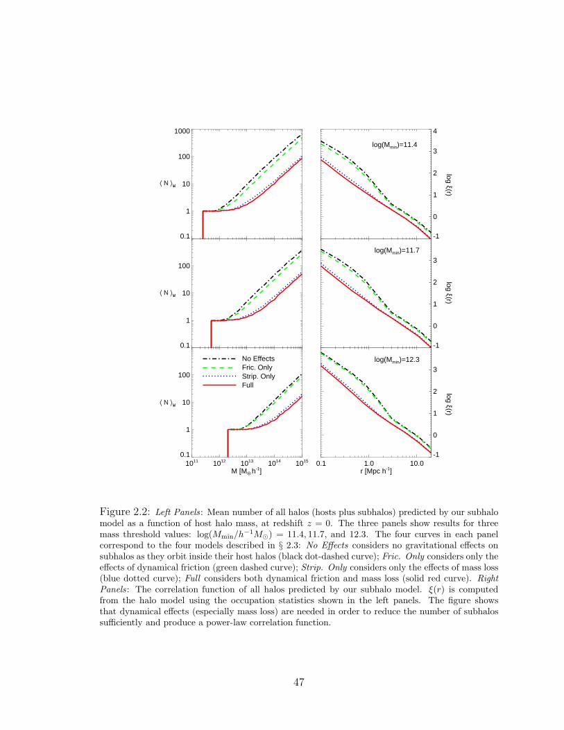
0.1

1

10

100

1000

-1

0

1

2

3

4

log ξ(r)

log(Mmin)=11.4

0.1

1

10

100

-1

0

1

2

3

log ξ(r)

log(Mmin)=11.7

1011 1012 1013 1014 1015

M [MO • h-1]

0.1

1

10

100

No EffectsFric. OnlyStrip. OnlyFull

0.1 1.0 10.0r [Mpc h-1]

log ξ(r)

-1

0

1

2

3log(Mmin)=12.3

Figure 2.2: Left Panels : Mean number of all halos (hosts plus subhalos) predicted by our subhalomodel as a function of host halo mass, at redshift z = 0. The three panels show results for threemass threshold values: log(Mmin/h

−1M⊙) = 11.4, 11.7, and 12.3. The four curves in each panelcorrespond to the four models described in § 2.3: No Effects considers no gravitational effects onsubhalos as they orbit inside their host halos (black dot-dashed curve); Fric. Only considers only theeffects of dynamical friction (green dashed curve); Strip. Only considers only the effects of mass loss(blue dotted curve); Full considers both dynamical friction and mass loss (solid red curve). Right

Panels : The correlation function of all halos predicted by our subhalo model. ξ(r) is computedfrom the halo model using the occupation statistics shown in the left panels. The figure showsthat dynamical effects (especially mass loss) are needed in order to reduce the number of subhalossufficiently and produce a power-law correlation function.

47

mass in the smoothed density distribution forms a galaxy and the galaxy can not be

destroyed. Of course, we expect the mean halo occupation in this model to be high

for all host masses as compared to the other models.

Next, we turn to the curves depicting the individual effects of dynamical friction

(Fric. Only, green dashed curves) and mass loss (Strip. Only, blue dotted curves).

These dynamical mechanisms can destroy subhalos, but they cannot affect the host

halo or central galaxy. This is why all the curves converge to the value 〈N〉M = 1 at

low host masses. As a convenient shorthand, we refer to any subhalo that fell into its

host system with a mass Msub ≥Mmin, but then merged with the central host galaxy

or lost sufficient mass to fall below this threshold, as destroyed. This does not mean

that the subhalo has become unbound, but merely that it has either merged or no

longer has a bound mass above some minimum mass threshold.

Dynamical friction acting alone destroys subhalos by causing them to sink to the

centers of their hosts and “merge” with it. This mechanism alone causes a 20-35%

decrease in the mean number of surviving satellites for all host masses as compared

to the No Effects model. The fractional decrease in subhalos depends only weakly

on host mass, but a comparison of the different mass threshold panels shows a mod-

est dependence on subhalo mass, with smaller mass subhalos being depleted more.

These trends are counter-intuitive because the dynamical friction force is an increas-

ing function of Msub/Mhost, the mass ratio between the subhalo and its host (Binney &

Tremaine, 2008). One might expect the depletion of subhalos to be larger for smaller

48

host masses at fixed subhalo mass or for larger subhalo masses at fixed host mass.

Our results differ from this expected behavior for two reasons. First and foremost,

low-mass-ratio mergers tend to occur at higher redshifts than high-mass-ratio merg-

ers. At higher redshifts, host halos are significantly smaller than they are at present,

so high-redshift mergers probe only the dense interiors of contemporary host halos

and evolve approximately according to the subhalo-host mass ratio at the redshift

of the merger. These early-merging subhalos also have a longer period of time dur-

ing which to evolve. Second, our models include subhalos-of-subhalos. As we move

to larger host masses at fixed subhalo mass or smaller subhalo masses at fixed host

mass, more subhalos are subs-of-subs that have much higher mass ratios with their

immediate hosts. These effects result in the trends we see in Figure 2.2.

Mass loss is significantly more effective at “erasing” subhalos than dynamical

friction. Mass loss processes can effectively “destroy” subhalos because many lose

sufficient mass to fall below the threshold of a sample. This mechanism typically

drives an 80-85% decrease in the number of objects above a given mass threshold

compared to the No Effects model. Again, the fractional decrease in subhalos is

nearly independent of host mass, but it shows a slight dependence on subhalo mass,

with smaller mass subhalos being destroyed more efficiently.

Finally, the Full model (red, solid curves) includes the effects of both subhalo

mass loss and orbital decay by dynamical friction. These processes do not simply

sum together. As a subhalo sinks deeper into its host potential well due to dynamical

49

friction, it experiences a stronger tidal field and is thus more efficiently stripped

of its mass. Conversely, less massive subhalos are less susceptible to orbital decay

via dynamical friction. A comparison of the Full model to the Strip. Only model

shows that including dynamical friction causes an additional ∼ 15% depletion of

substructure. Mass loss is by far the dominant cause of subhalo destruction. Overall,

Figure 2.2 shows that dynamical effects reduce the number of subhalos by ∼ 90%

compared to the number of distinct mergers that occur during the formation of a

host halo.

2.4.2 Constructing the Correlation Function

We use the halo model outlined in § 2.2 to compute the correlation function

predicted by our subhalo model. Specifically, we use the Jenkins et al. (2001) mass

function and we follow Tinker et al. (2005) in using the Smith et al. (2003) formula for

the non-linear matter power spectrum and the Tinker et al. (2005) scale-dependent

halo bias relative to the non-linear power spectrum. We derive HOD statistics from

our subhalo models as exemplified by the previous section, and we compute the pair

separation distributions by assuming that the radial distributions of satellites follows

an NFW profile for simplicity. In actuality, the subhalo distributions in both our

models and N -body simulations are slightly shallower than NFW (see Z05 for model

and simulation results). We adopt the NFW profile for analytical convenience as

deviations from NFW are small and only influence correlation functions notably on

50

scales significantly smaller than r ∼ 100h−1kpc (e.g., Z05; also see Watson et al. 2010

for a demonstration of this point regarding satellite galaxies).

The right column of Figure 2.2 shows the host+subhalo correlation functions

computed in this manner from the HODs predicted by our subhalo model. In the No

Effects case, where no subhalos are destroyed, ξ(r) is very different from a power law,

having a one-halo term that is too large relative to the two-halo term so that a distinct

feature is present in ξ(r) on scales r ∼ 2 Mpc. In fact, comparing this to Figure 2.1,

we see that it is very similar to the dark matter correlation function. This is perhaps

not surprising because subhalos in this model behave as massive test particles that

cannot be altered. As dynamical effects are included and substructure is consequently

depleted, ξ(r) drops on all scales. Recall that only subhalos (hosting satellite galaxies)

can be destroyed and the number of host galaxies remains unaltered. The fraction of

all objects that are satellites therefore decreases. As we discussed in § 2.2, for a fixed

population of central galaxies, the one-halo term drops in approximate proportion to

the number of satellite galaxies. So as the number of satellites declines, so does the

number of pairs within halos relative to the total number of pairs and the one-halo

term declines.

Large-scale clustering is less sensitive to changes in the satellite galaxy population.

The two-halo term drops because subhalos tend to populate more massive hosts (as

in the left column of Figure 2.2), so the average host halo mass of a sample decreases

as subhalos are depleted. The large-scale clustering strength of halos increases with

51

halo mass, so this depletion results in weaker large-scale clustering. The variability

of the two-halo term is relatively mild because the halo bias is not a rapidly-varying

function of halo mass near M ∼Mmin (Tinker et al., 2005).

With enough depletion of substructure, the one- and two-halo terms align and

result in a nearly power-law shape. This is exactly what happens in Figure 2.2. In

our Full subhalo model the correlation function is roughly a power law. To obtain

a nearly power-law galaxy correlation function, it is necessary that a majority of

early galaxies and proto-galaxies that merge to form a massive system at low redshift

be destroyed through either central mergers or mass loss. Our results suggest that

mass loss is mainly responsible for this depletion, while dynamical friction and central

galaxy mergers play a comparably small, supporting role. Incidentally, this picture

implies that infalling satellite galaxies lose significant stellar mass so that they provide

an important source of the diffuse intracluster light observed in galaxy groups and

clusters and this picture is consistent with observations (Purcell et al., 2007, 2008).

Comparing our correlation function results for the three different mass thresholds, we

note that ξ(r) is closer to a power law for lower-mass samples. We revisit this point

in the next section.

We now return to the mean occupation statistics shown in the left panels of Fig-

ure 2.2. The so-called “plateau” region of the HOD is the flat region at 〈N〉M = 1,

where host halos are more massive than Mmin, but not yet massive enough to host

52

subhalos above our mass threshold 3. As substructure is depleted, the prominence of

this plateau increases. The “length” of the plateau in the HOD can be expressed as

the ratio between the mass of a halo that hosts a single satellite on average, M1, to

the minimum mass required to host a central galaxy, Mmin. Zehavi et al. (2005b) fit

an HOD model to the measured correlation function of SDSS galaxies and found that

a ratio M1/Mmin ∼ 23 is consistent with clustering data, nearly independent of galaxy

luminosity. In other words, a consistent picture is one in which the entire HOD shifts

to higher masses in a self-similar manner, with M1/Mmin fixed, in order to accom-

modate higher-luminosity samples. Remarkably, Kravtsov et al. (2004a) studied this

for subhalos in a high-resolution N -body simulation and found that M1/Mmin ∼ 20,

regardless of Mmin as well. Meanwhile, Tinker et al. (2005) fit a slightly more complex

HOD model to the SDSS data and found that M1/Mmin ∼ 25 for galaxy samples with

luminosities less than L∗, but decreases to M1/Mmin . 5 to accommodate the highest-

luminosity samples (absolute r-band magnitudes Mr ≤ −21). The new analysis by

Zehavi et al. (2011) also finds this trend with M1/Mmin ∼ 17 for Mr ≥ −20.5 and

much lower values for higher luminosity galaxies. For the purpose of comparison, the

Full subhalo model shown in Figure 2.2 predicts M1/Mmin ∼ 40 for the low-mass sam-

ples of log(Mmin/h−1M⊙) = 11.4 and log(Mmin/h

−1M⊙) = 11.7, and M1/Mmin ∼ 30

for the higher-mass sample of log(Mmin/h−1M⊙) = 12.3.

3Roughly speaking, the most massive subhalo within any host is a few percent of the mass ofthe host halo (e.g., Z05). This is the case with, for example, the Large Magellanic Cloud within thehalo of the Milky Way (Busha et al., 2010).

53

These results suggest that getting the length of the HOD plateau right may be

a key ingredient needed to establish a power-law correlation function and this has

been part of the interpretation in the literature. The importance of M1/Mmin stems

from the fact that most one-halo pairs reside in halos with average satellite numbers

〈Ns〉M . 1, so modeling the HOD at relatively low satellite occupation numbers is

critical (see Conroy et al., 2006). We investigate this further in § 2.6.

2.5 Mass and Redshift Dependence of the Correlation Function

2.5.1 Dependence on Mass

While dynamical processes act in a manner to deplete substructure and push ξ(r)

toward a power law at all mass thresholds, it is evident that deviations from a power

law are stronger with increasing host mass. Figure 2.3 shows the correlation functions

predicted by our Full subhalo model for four different mass thresholds, ranging from

log(Mmin/h−1M⊙) = 13.5, corresponding to bright galaxies such as Luminous Red

Galaxies (LRGs), down to log(Mmin/h−1M⊙) = 10.5, corresponding to dwarf galaxies.

While the correlation function of the “dwarf” sample is a near power law, that of the

“LRG” sample exhibits strong departures from power-law behavior. This trend has

been detected with SDSS galaxies by Zehavi et al. (2005b) who found evidence that a

power-law model provides a better fit to low-luminosity galaxies than high-luminosity

galaxies. Halo and subhalo clustering exhibits the same trend. More massive halos

contain slightly more of their bound masses in substructure relative to less massive

54

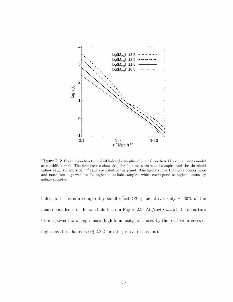
0.1 1.0 10.0r [ Mpc h-1 ]

-1

0

1

2

3

4

log

ξ(r)

log(Mmin)=13.5log(Mmin)=12.5log(Mmin)=11.5log(Mmin)=10.5

Figure 2.3: Correlation function of all halos (hosts plus subhalos) predicted by our subhalo modelat redshift z = 0. The four curves show ξ(r) for four mass threshold samples and the thresholdvalues Mmin (in units of h−1M⊙) are listed in the panel. The figure shows that ξ(r) breaks moreand more from a power law for higher mass halo samples, which correspond to higher luminositygalaxy samples.

halos, but this is a comparably small effect (Z05) and drives only ∼ 30% of the

mass-dependence of the one-halo term in Figure 2.3. At fixed redshift, the departure

from a power-law at high mass (high luminosity) is caused by the relative rareness of

high-mass host halos (see § 2.2.2 for interpretive discussion).

55

2.5.2 Dependence on Redshift

Substructure abundances vary with time. Infall of new subhalos acts as a “source”

of halo substructure. The rate of mergers of halos into larger systems is a function of

redshift that typically peaks at redshifts z ∼ 1− 3 in the halo mass range of interest

and declines thereafter (Z05; Zentner 2007). Once a subhalo merges into a larger host

halo, dynamical friction shrinks its orbit and the subhalo loses mass. Given enough

time, the subhalo will eventually lose enough mass to fall below Mmin or merge with

the central galaxy and lose its identity. The balance between the halo merger rate and

the rates of destructive processes (which occur on a halo dynamical time) determine

the redshift dependence of halo substructure.

Figure 2.4 shows the redshift evolution of the mean halo occupation number and

resulting correlation functions. The layout of Figure 2.4 is similar to that of Fig-

ure 2.2, with 〈N〉M shown in the left panels, ξ(r) shown in the right panels. However,

in Figure 2.4 all results are for the Full subhalo model, and the various lines denote

quantities evaluated at different redshifts, z = 3, 1, 0, −0.6, −0.9 (where nega-

tive redshifts correspond to future epochs). Moreover, in each panel the correlation

functions are scaled by a power law to better highlight departures from a power-law

shape.

The left-hand panels of Figure 2.4 show that the average number of subhalos

within hosts of a given mass starts out high at early times and begins to decrease

after z = 3, as merger rates decline. By the present epoch (z = 0), the number of

56

subhalos has dropped by ∼ 25−30% relative to what it was at z = 3. One Hubble time

into the future (z = −0.6), the abundance of substructure has dropped by ∼ 60%.

This is because the rate of merging as a source for new subhalos declines rapidly. This

decrease in the merger rate is dictated in large part by the quenching of structure

growth by the cosmological constant (Carroll et al., 1992), but also because most halos

of interest are below the typical collapsing mass, which approaches M∗ ≃ 1014 h−1M⊙

in the future (Zentner, 2007). Meanwhile, destructive processes continue to operate

on orbiting halo substructure for several additional dynamical times. Three Hubble

times into the future (z = −0.9) the average halo occupation has dropped by ∼ 90%.

As with our previous results, the fractional decrease in subhalo abundance appears to

be roughly independent of host mass, meaning that the slope of the HOD in the high-

〈N〉M limit is not significantly altered by evolution. The amplitude of 〈N〉M declines

considerably, resulting in increasing M1/Mmin, or a “lengthening” of the HOD plateau

with time. This behavior is strikingly similar to that seen in Figure 2.2 in the sense

that turning on dynamical effects at a fixed redshift has a qualitatively similar impact

as evolving forward in time, and the effects on the correlation function are similar.

Turning to the right panels, ξ(r) is shown at each redshift scaled by an r−1.7 power

law in order to emphasize features in the correlation function. Starting at z = 3 (long

dashed curves), ξ(r) is very far from a power-law, with a slope that is much steeper

on small scales. At z = 1 (short dashed curves) the break from a power law is less

pronounced, but it is still significant. These results are qualitatively consistent with

57

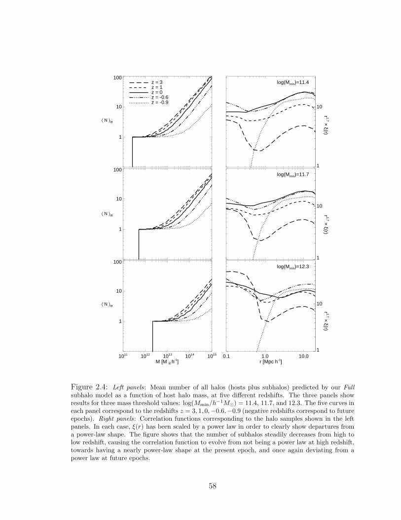
1

10

100z = 3z = 1z = 0z = -0.6z = -0.9

1

10

r 1.7 × ξ(r)log(Mmin)=11.4

1

10

100

1

10

r 1.7 × ξ(r)

log(Mmin)=11.7

1011 1012 1013 1014 1015

M [M O • h-1]

1

10

100

0.1 1.0 10.0r [Mpc h-1]

1

10

r 1.7 × ξ(r)

log(Mmin)=12.3

Figure 2.4: Left panels : Mean number of all halos (hosts plus subhalos) predicted by our Full

subhalo model as a function of host halo mass, at five different redshifts. The three panels showresults for three mass threshold values: log(Mmin/h

−1M⊙) = 11.4, 11.7, and 12.3. The five curves ineach panel correspond to the redshifts z = 3, 1, 0,−0.6,−0.9 (negative redshifts correspond to futureepochs). Right panels : Correlation functions corresponding to the halo samples shown in the leftpanels. In each case, ξ(r) has been scaled by a power law in order to clearly show departures froma power-law shape. The figure shows that the number of subhalos steadily decreases from high tolow redshift, causing the correlation function to evolve from not being a power law at high redshift,towards having a nearly power-law shape at the present epoch, and once again deviating from apower law at future epochs.

58

clustering measurements at high redshifts (Coil et al., 2006; Ouchi et al., 2005; Lee

et al., 2006). At z = 0 (solid curves), the correlation function is approximately a

power law, though there is still a mild, discernible feature at the transition scale

between the one- and two-halo terms. In the future, ξ(r) once again breaks from a

power law. At z = −0.6 (dot-dashed curves), departures from a power-law shape

are about as strong as they were at z = 1. Three Hubble times into the future,

at z = −0.9 (dotted curves), the departures from a power law are significant and

represent a dramatic reduction in the relative contribution of the one-halo term.

Figure 2.5 focuses on the log(Mmin/h−1M⊙) = 12.3 threshold sample and shows

the correlation function at four different redshifts, while also showing the one-halo

and two-halo terms explicitly. Figure 2.5 clearly demonstrates how a delicate balance

is needed between the two terms in order for ξ(r) to achieve a power-law shape. The

two-halo term exhibits modest variations from panel to panel, with a range of about a

factor of ∼ 3. The decreased large-scale clustering at z & 0 is due to the linear growth

of perturbations with time, but this is always kept modest because the increasing bias

of halos of fixed mass with redshift (see Zentner, 2007) compensates for large-scale

structure growth. At z < 0, the slight decrease in two-halo clustering is due to the

decay of halo bias once halo growth slows (Fry, 1996).

The variation in the one-halo term is significantly larger, as our earlier discussions

suggest, and changes by a factor of ∼ 45 − 150 (depending on scale), equivalent to

∼ 15 − 50 times the variation in the two-halo term. At high redshift, the relative

59

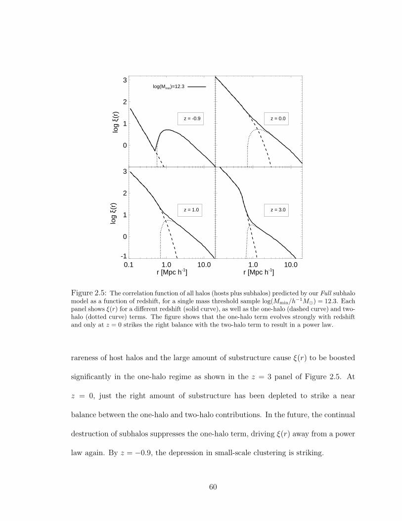
0

1

2

3

log

ξ(r)

log(Mmin)=12.3

z = -0.9

z = 0.0

0.1 1.0 10.0r [Mpc h-1]

-1

0

1

2

3

log

ξ(r)

z = 1.0

1.0 10.0r [Mpc h-1]

z = 3.0

Figure 2.5: The correlation function of all halos (hosts plus subhalos) predicted by our Full subhalomodel as a function of redshift, for a single mass threshold sample log(Mmin/h

−1M⊙) = 12.3. Eachpanel shows ξ(r) for a different redshift (solid curve), as well as the one-halo (dashed curve) and two-halo (dotted curve) terms. The figure shows that the one-halo term evolves strongly with redshiftand only at z = 0 strikes the right balance with the two-halo term to result in a power law.

rareness of host halos and the large amount of substructure cause ξ(r) to be boosted

significantly in the one-halo regime as shown in the z = 3 panel of Figure 2.5. At

z = 0, just the right amount of substructure has been depleted to strike a near

balance between the one-halo and two-halo contributions. In the future, the continual

destruction of subhalos suppresses the one-halo term, driving ξ(r) away from a power

law again. By z = −0.9, the depression in small-scale clustering is striking.

60

Some of the evolution of ξ(r) on small-scales comes from the fact that halos large

enough to host luminous galaxies become increasingly rare as redshift increases. The

characteristic collapsing mass is a rapidly decreasing function of redshift and is only

M∗ ≈ 109 h−1M⊙ at z = 3. In the relevant regime, the strength of the one-halo term

grows in approximate proportion to the number of satellite galaxies and in inverse

proportion to the number of host halos of appropriate size (see § 2.2), so the relative

paucity of host halos at high redshift also drives strong one-halo clustering because

Fig. 2.5 describes samples of fixed absolute mass threshold. However, it is subhalo

abundance that has the larger influence on the redshift dependence of clustering. We

have computed the correlations of Figure 2.5 using samples in which Mmin varies with

redshift so as to maintain a constant number density of halos. These samples are less

subject to the gross evolution of the halo mass function. We find all of the same

qualitative results for this case, though the two-halo term varies by a factor of ∼ 4,

while the variation in the one-halo term is limited to a factor of ∼ 12 − 80 (again,

depending on scale), resulting in a variation in the one-halo term that is ∼ 3−20 times

larger than that of the two-halo term. Moreover, we have re-computed correlation

functions using a combination of the predicted low-redshift HODs alongside the high-

redshift mass functions in order to isolate the contribution due to the mass function

and HOD evolution. The majority the redshift dependence of ξ(r) on small scales

is due to the evolution of subhalo abundance. To maintain a power-law correlation

function at high-redshift would require fewer subhalos per host than at z = 0 in order

61

to compensate for the relative rareness of host halos at high-redshift. In fact, hosts

at high redshift have a larger number of subhalos of any given mass so these effects

reinforce one another, leading to a strong deviation from a power-law ξ(r) at high

redshift.

We have already described the reasons that the one-halo and two-halo terms be-

have so differently under changes in the HOD. To reiterate, on large scales, ξ(r) is

essentially a weighted average of the clustering of host halos, where 〈N〉M provides

the weighting (see the integral in Eqs. [2.6] and [2.7], note that λ(k,M) ≈ 1 for

k < 1/Rvir). The possible variability in ξ(r) on large scales is limited because it is

always bound by the limited variation in the clustering of host halos. As we discussed

in § 2.2, the difference in the large-scale bias of the largest relative to the smallest

halos is at most a factor of ∼ 3 (e.g., Tinker et al. 2005). Significant variations in

large-scale clustering require dramatic variations in the HOD at high mass, which

are not expected on theoretical grounds and are not mandated by data. However,

on scales smaller than the size of individual host halos, ξ(r) can vary dramatically

depending on the HOD. For example, in the extreme case of only one object per host

halo, there will be zero pairs within halos and the one-halo term will vanish. For large

numbers of satellites, the one-halo term will be significantly larger than a power-law

extrapolation of the two-halo term to small scales.

The sensitivity of the one-halo term to the HOD, coupled with the relative insen-

sitivity of the two-halo term, means that achieving a power-law correlation function

62

requires fine-tuning in the number of satellite galaxies per halo. The satellite galaxy

abundance naturally evolves with redshift, so ξ(r) can only be a power law during

those epochs when substructure has evolved to join the one-halo term to the two-halo

term. Of course, it may be possible for features in the host halo mass function or

bias relations to conspire to compensate for substructure evolution, but such features

would somehow need to be coordinated with low-redshift structure growth. A different

way to state this is that the halo mass function and halo bias depend on the statistics

of the linear density field, and do not “know” about the non-linear galaxy formation

and gravitational processes that occur within halos. It would be quite strange if their

evolution were somehow connected with the evolution of satellite galaxies in virialized

hosts. It seems to be a coincidence that the epoch of near power-law clustering of

typical galaxies lies near z = 0.

2.5.3 The Balance Between Accretion and Destruction

We have just seen how the depletion of substructure over time leads to evolution

in the correlation function such that it becomes a power law at the present epoch.

However, what drives substructure depletion? We expect that most subhalos will lose

significant amounts of mass or merge with the central galaxy given sufficient time.

However, this will be compensated to some degree by the infall of new subhalos. If

the rate at which satellites are accreted is greater than the rate at which they are

destroyed, then the net amount of substructure will grow with time. The evolution in

63

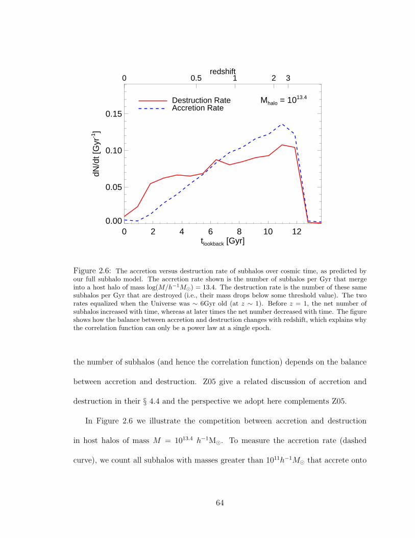
0 2 4 6 8 10 12tlookback [Gyr]

0.00

0.05

0.10

0.15

dN/d

t [G

yr-1]

0 0.5 1 2 3redshift

Destruction RateAccretion Rate

Mhalo = 1013.4

Figure 2.6: The accretion versus destruction rate of subhalos over cosmic time, as predicted byour full subhalo model. The accretion rate shown is the number of subhalos per Gyr that mergeinto a host halo of mass log(M/h−1M⊙) = 13.4. The destruction rate is the number of these samesubhalos per Gyr that are destroyed (i.e., their mass drops below some threshold value). The tworates equalized when the Universe was ∼ 6Gyr old (at z ∼ 1). Before z = 1, the net number ofsubhalos increased with time, whereas at later times the net number decreased with time. The figureshows how the balance between accretion and destruction changes with redshift, which explains whythe correlation function can only be a power law at a single epoch.

the number of subhalos (and hence the correlation function) depends on the balance

between accretion and destruction. Z05 give a related discussion of accretion and

destruction in their § 4.4 and the perspective we adopt here complements Z05.

In Figure 2.6 we illustrate the competition between accretion and destruction

in host halos of mass M = 1013.4 h−1M⊙. To measure the accretion rate (dashed

curve), we count all subhalos with masses greater than 1011h−1M⊙ that accrete onto

64

these hosts in finite time intervals. For the destruction rate (solid curve), we count the

number of these same subhalos that drop below 1011h−1M⊙ during the time intervals.

The accretion rate minus the destruction rate will then give us the net rate of change

in the number of subhalos per unit time.

Figure 2.6 shows that the accretion rate quickly grew and reached a peak at

z ∼ 2 − 3. Since this peak, the accretion rate has been steadily declining and is

close to zero at the present epoch. The decline in merger rates is partly due to the

shape of the power spectrum (see Lacey & Cole, 1993; Somerville & Kolatt, 1999;

Zentner, 2007), but the driving force for the recent fast decline in the merger rate of

halos is the reduced rate of structure growth caused by accelerated cosmic expansion.

The destruction rate also peaked at z ∼ 2 − 3 and lags the accretion rate because

most destruction happens over a period of several dynamical times. Figure 2.6 clearly

shows that the accretion rate has been dropping faster than the destruction rate since

their peaks, with accretion and destruction roughly balancing just below z ∼ 1 (see

also Stewart et al., 2009). This means that the number of subhalos in hosts that

grow to a mass of M = 1013.4 h−1M⊙ by z = 0 increased until z ≈ 1 and has been

declining ever since, despite the fact that the virial masses of these halos have been

growing. The general trend toward reduced substructure at low redshift explains the

behavior exhibited in Figure 2.4. The correlation function is close to a power law at

the present epoch because the balance between accretion and destruction over time

has led to the requisite abundance of substructure today.

65

2.6 Achieving a Power-Law Correlation Function

We now step back from making predictions using our specific subhalo model and

undertake a general exploration of the properties of the HOD that yield nearly power-

law correlation functions at different masses and redshifts. The HOD characterizes the

number and spatial distribution of galaxies within dark matter halos. It is typically

specified with a handful of parameters that are constrained using galaxy clustering

measurements (e.g., Magliocchetti & Porciani, 2003; Zehavi et al., 2005b; Tinker

et al., 2005; Zheng et al., 2007). We choose an HOD model that is motivated by

theoretical predictions from hydrodynamic simulations, semi-analytic models, and

high-resolution N-body simulations (Berlind et al., 2003; Kravtsov et al., 2004a; Zheng

et al., 2005). According to this model, halos above some threshold mass contain a

single “central” galaxy plus a number of “satellite” galaxies. The number of satellites

in any given halo is drawn from a Poisson distribution whose mean is a power-law

function of host halo mass. The central galaxy is placed at the center of the host halo,

while the satellites are spatially distributed according to an NFW density profile.

Specifically, we adopt an HOD parametrization that is similar to the one used by

Tinker et al. (2005). This is a simple, yet powerful model in which the number of

central galaxies is modeled as a step function,

Ncen =

1 if M ≥ Mmin

0 if M < Mmin

, (2.8)

66

while the mean number of satellites follows a power-law with an exponential cutoff

at low mass,

〈Nsat〉M =

(

M

M1

)α

exp

(

−M0

M

)

. (2.9)

The parameters in the model are as follows.

1. Mmin is the minimum host halo mass to contain a central galaxy.

2. M0 is the host halo mass below which satellite galaxies are exponentially sup-

pressed.

3. M1 is the host halo mass to contain, on average, one satellite galaxy.

4. α is the index of the power-law relation between the mean number of satellite

galaxies and halo mass.

Previous studies have shown that the power-law index α ≈ 1 for subhalos and

simulated galaxies (Kravtsov et al., 2004a; Zheng et al., 2005; Zentner et al., 2005),

as well as observed galaxies dimmer than L∗ (Zehavi et al., 2005b), leading Tinker

et al. (2005) to set α = 1 throughout their analysis. However, we allow α to vary

because the correlation function is sensitive to it and, although it may be near unity

when modeling observed data, it may need to deviate from unity to yield a power-law

correlation function at high redshifts. On the other hand, ξ(r) is not sensitive to M0,

consequently we fix its value by adopting the Conroy et al. (2006) M0 −M1 relation,

log(M0/h−1M⊙) = 0.76 log(M1/h

−1M⊙) + 2.3. (2.10)

67

The result is an HOD model with only three free parameters: Mmin, M1, and α.

The two-halo term of ξ(r) depends on the mean occupation 〈N〉M = 〈Ncen +

Nsat〉M , which is equal to 1+ 〈Nsat〉M for M > Mmin. The one-halo term also requires

the second moment of the occupation distribution 〈Nsat(Nsat−1)〉M , so characterizing

the mean occupation is not sufficient. We assume that the number of satellites follows

a Poisson distribution, for which 〈Nsat(Nsat − 1)〉M ≡ 〈Nsat〉2M . Our Full model devi-

ates mildly from a pure Poisson distribution (see Fig. 7 of Z05, and recent simulations

of Boylan-Kolchin et al., 2010, that find similar deviations from a Poisson distribu-

tion), but the effect of this deviation on ξ(r) is minor (Fig. 16 of Z05). We also note

that there are any number of possible parametrizations for 〈Nsat〉M to choose from

besides the one adopted here. We have found that mildly different parametrizations

that exhibit the same basic features and are consistent with contemporary data (e.g.,

the one used by Zehavi et al. 2005b) yield similar conclusions.

We consider the HOD parameter space that yields a power-law correlation func-

tion for three galaxy samples of fixed number density ng, at three different redshifts

z = 0, 1, 3. Fixing number density is a way to compare similar samples at different

redshifts because the high-redshift sample is more likely to represent the progeni-

tors of the low-redshift sample than it would in the case of mass threshold samples.

We choose number densities equal to ng = 0.02, 0.01, and 0.003 h3Mpc−3, which

correspond to three z ≃ 0, volume-limited, r-band threshold samples in the SDSS:

Mr < −18.5, −19.5, and −20.5 (Zehavi et al., 2005b).

68

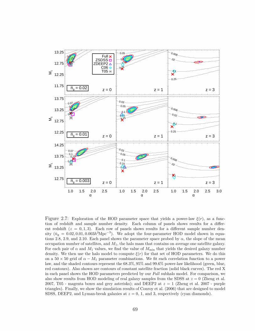
11.75

12.25

12.75

13.25M

1

0.1

0.15

0.25

ng = 0.02

FullZSDSS

ZDEEP2C06T05

z = 0

0.05

0.1

0.15

0.25

z = 1

z = 3

0.008

.02

0.1

0.25

α

12.25

12.75

13.25

13.75

M1

z = 0

0.07

0.10.15

0.25

ng = 0.01

0.03

0.05

0.1

0.150.25

z = 1

α

z = 3

0.008

0.02

0.1

0.25

1.0 1.5 2.0 2.5 α

12.75

13.25

13.75

14.25

M1

z = 0

0.070.10.15

0.25

ng = 0.003

1.0 1.5 2.0 2.5 α

0.030.05

0.10.150.25

z = 1

1.0 1.5 2.0 2.5 3.0α

0.008.02

0.1

z = 3

Figure 2.7: Exploration of the HOD parameter space that yields a power-law ξ(r), as a func-tion of redshift and sample number density. Each column of panels shows results for a differ-ent redshift (z = 0, 1, 3). Each row of panels shows results for a different sample number den-sity (ng = 0.02, 0.01, 0.003h3Mpc−3). We adopt the four-parameter HOD model shown in equa-tions 2.8, 2.9, and 2.10. Each panel shows the parameter space probed by α, the slope of the meanoccupation number of satellites, and M1, the halo mass that contains on average one satellite galaxy.For each pair of α and M1 values, we find the value of Mmin that yields the desired galaxy numberdensity. We then use the halo model to compute ξ(r) for that set of HOD parameters. We do thison a 50 × 50 grid of α −M1 parameter combinations. We fit each correlation function to a powerlaw, and the shaded contours represent the 68.3%, 95% and 99.6% power-law likelihood (green, blue,red contours). Also shown are contours of constant satellite fraction (solid black curves). The red Xin each panel shows the HOD parameters predicted by our Full subhalo model. For comparison, wealso show results from HOD modeling of real galaxy samples from the SDSS at z = 0 (Zheng et al.2007, T05 - magenta boxes and grey asterisks); and DEEP2 at z = 1 (Zheng et al. 2007 - purpletriangles). Finally, we show the simulation results of Conroy et al. (2006) that are designed to modelSDSS, DEEP2, and Lyman-break galaxies at z = 0, 1, and 3, respectively (cyan diamonds).

69

For a given number density and redshift combination (e.g., ng = 0.02 h3Mpc−3 at

z = 1), we create a 50× 50 grid of M1 − α parameter combinations. For each pair of

M1 and α on this grid, we use Equation (2.3) to find the value of Mmin that is needed

to enforce the desired number density. In this manner, the 2,500 HOD models on the

grid represent galaxy samples with the same number densities, but different HODs.

We then compute the first and second moments of the mean galaxy occupation using

equations (2.8) and (2.9), and use the halo model described in § 2.2 to construct

ξ(r). We assign 10% errors on all scales to ξ(r), as such errors are roughly consistent

with jackknife re-sampling errors in current clustering measurements (Zehavi et al.,

2005b), and we fit a power-law function to all 2,500 correlation functions. We perform

our fits using a Markov Chain Monte Carlo (MCMC) analysis in which we vary the

slope and correlation length of the fitted power-law. We then find the minimum χ2

value for a power-law fit to ξ(r) for any given M1 −α combination. This allows us to

approximate the HOD parameter space in which ξ(r) is consistent with a power law

at a level similar to contemporary observations. For two free parameters, the 68.3%

(1σ), 95% (2σ), and 99.6% (3σ) likelihood regions correspond to values of reduced

χ2 ≤ 1.15, 1.61, and 2.06, respectively.

Figure 2.7 shows the contours generated from the aforementioned procedure. Each

row in the figure represents a different ng value and each column corresponds to a

different redshift. The “satellite fraction” (fsat, the fraction of all galaxies that are

satellites, see Eq. [2.5]) is relevant to the shape of the galaxy two-point correla-

70

tion function. Therefore, over-plotted in each panel are curves of constant fsat (the

labeled, solid, black curves). To compare these results with measurements from ob-

served galaxies, in each panel we also show best-fit M1 and α values from published

halo model fits to measurements of ξ(r) using galaxy samples with the same number

densities at the same redshifts. Squares and triangles represent the best-fit parame-

ter values from Zheng et al. (2007) who fit SDSS (z = 0) and DEEP2 (z = 1) data

(ZSDSS, ZDEEP2) and asterisks represent the best-fit Tinker et al. (2005) values for

SDSS data (T05). Diamonds represent the Conroy et al. (2006) values for SDSS,

DEEP2, and the z = 3 Subaru data of Lyman-break galaxies (C06).

The best-fit parameter combinations should be regarded as best-fit “regions”,

because there are errors associated with the derived parameters (e.g., the Zheng et al.

(2007) SDSS α and M1 errors at each luminosity are of order 10%). We note that

Tinker et al. (2005) considered several possible values of σ8, but we show their results

for σ8 = 0.9 to be consistent with the cosmological model used in the other studies.

Finally, in each panel we show the HOD parameters predicted by our Full subhalo

model (marked by an “X”) for samples with mass thresholds that yield the desired

number density. The Full model gives 〈Nsat〉M and we fit this with Equation (2.9) to

obtain best-fit values of M1 and α.

Several interesting conclusions can be drawn from this figure.

1. The region of HOD parameter space that yields a power-law ξ(r) drifts to

lower values of both M1 and α with increasing number density. These trends

71

increase the satellite fraction as number density increases to compensate for the

relative reduction in the one-halo term compared to the two-halo term induced

by moving to a lower-mass, more abundant halo sample.

2. The values of α that result in the best power laws drift higher with increasing

redshift in an effort to boost the two-halo term by placing galaxies in massive,

highly-biased halos. In general, it is difficult to arrange a power law at z ≥ 3

for these three number densities.

3. As might be expected from our previous discussions, there is a relatively narrow

range of fsat for the best-fit power-law space at each redshift. At z = 0, the

space that is consistent with a power-law with 10% errors on the data lie near

fsat ∼ 0.1 − 0.15. The direct fits to observational data lie near fsat = 0.2 − 0.3.

At z = 1, the power-law region is shifted to fsat ∼ 0.05 − 0.1, while at z = 3

the power-law region is even lower, fsat ∼ 0.01 − 0.02. Note that the power-

law regions are not precisely aligned along constant-fsat contours, particularly

at low redshift and low number density, indicating that other factors, such as

host halo abundances and the physical sizes of host halos, contribute to the

power-law nature of ξ(r). However, at high redshift and low number density,

the power-law regions become more nearly co-linear with contours of constant

fsat over a range of α values.

72

4. The SDSS (z ∼ 0) best-fit points lie near the power-law contours, but not within

these likelihood regions. This is not surprising as the SDSS measurement is more

precise over a wide range of scales than the ∼ 10% errors we have assumed and

the observed ξ(r) is now known to exhibit very small, but statistically-significant

deviations from a power law (Zehavi et al., 2004).

5. As predicted from Figure 2.3, the fits to observational data lie further from

the power-law regions as we move to lower ng (higher luminosity) samples. At

fixed redshift, this is driven largely because the host halos of these galaxies

become increasingly rare. However, it is worth noting that the growth of the

one-halo term with increasing Mmin is reinforced by an increase in satellite

abundance at fixed scaled mass Msub/Mhost as Mhost increases, accounting for ∼

30% of the rise. This increase satellite abundance withMhost arises because more

massive host halos assemble more recently, leaving less time for the evolution

of substructure and less satellite destruction (Z05). The relative time available

for satellite evolution is an important part of determining the power-law nature

of the correlation function.

6. The fits to observational data lie near the power-law regions at z = 0, but grow

more distinctly separated with increasing redshift. This evolution is driven by

satellite fractions at high-z that are too large to be consistent with power-law

clustering. This supports our basic picture that satellite destruction over cosmic

time is needed to achieve a power law ξ(r), and that the observed low-luminosity,

73

low-redshift ξ(r) is a coincidence.

7. The HOD values predicted by our Full subhalo model are similar to all of

the observed data fits at all redshifts. This is a remarkable result considering

our model treats only subhalos and not galaxies explicitly. We explore more

complicated associations of galaxies and subhalos in a follow-up study.

8. Our subhalos, as well as all observational data, reveal values of α ≃ 1 for all

redshifts, in accord with previous theoretical results (Kravtsov et al., 2004a;

Zheng et al., 2005; Zentner et al., 2005; Conroy et al., 2006). Moreover, at

each redshift, they have fixed satellite fractions, independent of ng. At z = 0,

z = 1, and z = 3, our model and the observational data cluster near fsat ≈ 0.25,

fsat ≈ 0.2, and fsat ≈ 0.1, respectively. We note that the lower satellite fractions

at high redshift are not due to HOD evolution. Figure 2.4 shows that 〈Nsat〉

is higher at high z. Instead, satellite fractions are lower at high z because all

relevant host halos have Mhost > M∗ and lie on the exponentially-decreasing

portion of the halo mass function, so the relative number of M1-mass host

halos to Mmin-mass halos decreases with redshift. Nevertheless, these satellite

fractions at high redshift are too high to support a power-law galaxy correlation

function.

9. Figure 2.7 implies that the physical mechanisms that dictate the HOD of galax-

ies operate to maintain α and fsat approximately fixed and not to achieve a

74

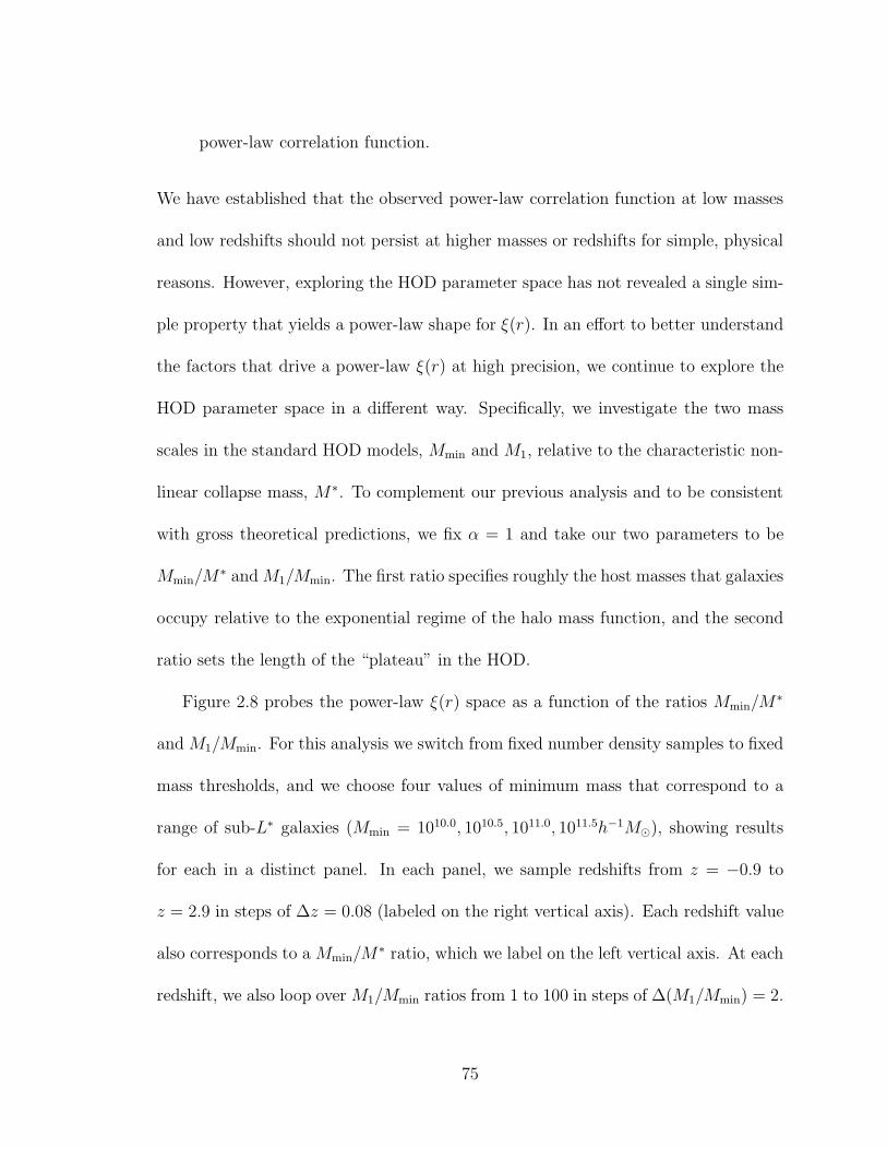
power-law correlation function.

We have established that the observed power-law correlation function at low masses

and low redshifts should not persist at higher masses or redshifts for simple, physical

reasons. However, exploring the HOD parameter space has not revealed a single sim-

ple property that yields a power-law shape for ξ(r). In an effort to better understand

the factors that drive a power-law ξ(r) at high precision, we continue to explore the

HOD parameter space in a different way. Specifically, we investigate the two mass

scales in the standard HOD models, Mmin and M1, relative to the characteristic non-

linear collapse mass, M∗. To complement our previous analysis and to be consistent

with gross theoretical predictions, we fix α = 1 and take our two parameters to be

Mmin/M∗ andM1/Mmin. The first ratio specifies roughly the host masses that galaxies

occupy relative to the exponential regime of the halo mass function, and the second

ratio sets the length of the “plateau” in the HOD.

Figure 2.8 probes the power-law ξ(r) space as a function of the ratios Mmin/M∗

and M1/Mmin. For this analysis we switch from fixed number density samples to fixed

mass thresholds, and we choose four values of minimum mass that correspond to a

range of sub-L∗ galaxies (Mmin = 1010.0, 1010.5, 1011.0, 1011.5h−1M⊙), showing results

for each in a distinct panel. In each panel, we sample redshifts from z = −0.9 to

z = 2.9 in steps of ∆z = 0.08 (labeled on the right vertical axis). Each redshift value

also corresponds to a Mmin/M∗ ratio, which we label on the left vertical axis. At each

redshift, we also loop over M1/Mmin ratios from 1 to 100 in steps of ∆(M1/Mmin) = 2.

75

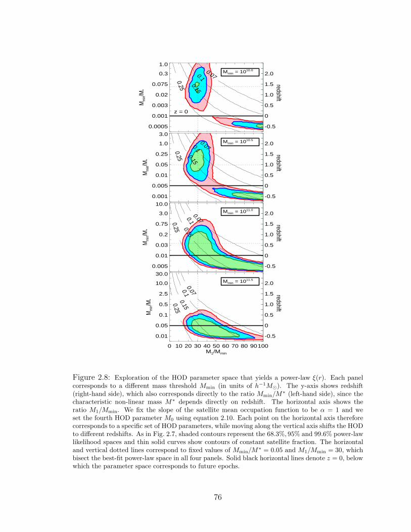
M1/Mmin

0.0005

0.001

0.003

0.02

0.075

0.3

1.0

Mm

in/M

*

z = 0

-0.5 0 0.5 1.0 1.5 2.0

redshift

0.070.1

0.15

0.25

Mmin = 1010.0

M1/Mmin

0.001

0.005

0.01

0.05

0.25

1.0

3.0

Mm

in/M

*

-0.5 0 0.5 1.0 1.5 2.0

redshift0.070.1

0.15

0.25

Mmin = 1010.5

M1/Mmin

0.005

0.01

0.03

0.2

0.75

3.0

10.0

Mm

in/M

*

-0.5 0 0.5 1.0 1.5 2.0

redshift

0.070.10.15

0.25

Mmin = 1011.0

0 10 20 30 40 50 60 70 80 90100M1/Mmin

0.01

0.05

0.1

0.5

2.5

10.0

30.0

Mm

in/M

*

-0.5 0 0.5 1.0 1.5 2.0

redshift

0.070.10.150.25

Mmin = 1011.5

Figure 2.8: Exploration of the HOD parameter space that yields a power-law ξ(r). Each panelcorresponds to a different mass threshold Mmin (in units of h−1M⊙). The y-axis shows redshift(right-hand side), which also corresponds directly to the ratio Mmin/M

∗ (left-hand side), since thecharacteristic non-linear mass M∗ depends directly on redshift. The horizontal axis shows theratio M1/Mmin. We fix the slope of the satellite mean occupation function to be α = 1 and weset the fourth HOD parameter M0 using equation 2.10. Each point on the horizontal axis thereforecorresponds to a specific set of HOD parameters, while moving along the vertical axis shifts the HODto different redshifts. As in Fig. 2.7, shaded contours represent the 68.3%, 95% and 99.6% power-lawlikelihood spaces and thin solid curves show contours of constant satellite fraction. The horizontaland vertical dotted lines correspond to fixed values of Mmin/M

∗ = 0.05 and M1/Mmin = 30, whichbisect the best-fit power-law space in all four panels. Solid black horizontal lines denote z = 0, belowwhich the parameter space corresponds to future epochs.

76

For every pair of Mmin/M∗ and M1/Mmin values, we compute ξ(r) using the halo

model and fit a power-law function in the same fashion as described previously. As

before, we show the 68.3%, 95% and 99.6% likelihood regions of ξ(r) consistent with

a power law (green, blue, and red contours, respectively). Also, as before, we show

contours of constant satellite fraction, fsat (solid black curves). The thick horizontal

lines at z = 0 are meant to emphasize that the parameter space lying below these

lines corresponds to future epochs.

We have repeated this analysis for higher mass thresholds (values of Mmin =

1012.0, 1012.5, 1013.0, 1013.5h−1M⊙). However, we do not show those results because

we found no parameter combinations within the 99.6% power-law likelihood space.

Figure 2.7 showed that the power-law parameter space drifted to higher values of α

for lower number density (and hence higher mass) samples in an effort to drive up the

two-halo term to meet the enhanced one-halo term. Therefore, it is not surprising

that we do not find this space when we restrict the slope to be α = 1.

Many interesting results can be drawn from Figure 2.8. Again, we itemize them

for the sake of clarity.

1. In order for ξ(r) to have a shape consistent with a power-law assuming ∼ 10%

measurement errors, it appears necessary for the “plateau” in the HOD to be

sufficiently long. At all masses and redshifts, M1/Mmin needs to be at least

∼ 20, otherwise the large satellite fraction drives a one-halo term that is too

large relative to the two-halo term. Moreover, for past epochs, z > 0, the

77

maximum plateau length is M1/Mmin . 40. Higher values of M1/Mmin yield

a one-halo term that is too weak. In fact, M1/Mmin ∼ 30 seems to be the

preferred value to yield a nearly power-law correlation function at all masses

so long as z > 0. This value is denoted by the vertical dotted lines in all the

panels.

2. For z ≥ 0, a near power-law ξ(r) seems to require a restricted range ofMmin/M∗.

Interestingly, the value Mmin/M∗ ∼ 0.05 can yield a power-law correlation func-

tion at all masses for appropriate choices of redshift. This value is denoted

by the horizontal dotted lines in all the panels. This restriction on Mmin/M∗

means that higher redshift samples (when M∗ is significantly smaller than to-

day) can only exhibit power-law behavior if the relevant host halos are signifi-

cantly smaller. This possibility becomes irrelevant in a practical sense because

star formation is inefficient in small halos (M ≪ 1011h−1M⊙, e.g., Conroy &

Wechsler, 2009; Behroozi et al., 2010; Guo et al., 2010)), so they cannot host

galaxies that are easily observable at high redshift. Figure 2.8 shows that the

lowest-mass samples that we consider (top two panels) have a nearly power-law

ξ(r) at 1 . z . 2, whereas the highest-mass samples have a nearly power-law

ξ(r) only at low redshift.

3. At sufficiently high redshift, near power-law clustering is no longer achievable at

any mass threshold corresponding to relatively bright galaxies. Our results gen-

erally indicate that power-law clustering at high redshift can only be achieved

78

if galaxies at high redshift occupy halos in a markedly different and more com-

plicated manner than their low-z counterparts.

4. For future epochs these broad results no longer hold. A broader range of

M1/Mmin values can be made approximately consistent with a power law at

low values of Mmin/M∗, or low/negative redshifts. For the lowest Mmin samples

the power-law likelihood space is clearly bimodal, with possible ways to achieve

a power law both at high redshifts and at low/future redshifts.

5. At all masses and redshifts we find that the power-law likelihood parameter

space has satellite fractions in the range fsat ∼ 0.1 − 0.25, with the fsat = 0.15

contour slicing through all of the 1σ regions. fsat is naturally strongly dependent

on both M1/Mmin and Mmin/M∗. Increasing the length of the HOD plateau at

fixed Mmin and redshift makes fsat decrease, as does boosting Mmin/M∗ while

keeping Mmin and the plateau fixed. If we keep both ratios fixed (i.e., both the

HOD shape and its position relative to the mass function) then the satellite

fraction is also approximately fixed, regardless of Mmin.

2.7 Discussion & Primary Conclusions

It has been recognized for decades that the two-point correlation function has a

simple, power-law form with ξ(r) ∼ r−2. Observational determinations of galaxy two-

point clustering spanning more than thirty years all yielded results consistent with a

single power law extending from linear and quasi-linear length scales (r & 30 h−1Mpc)

79

to deeply non-linear scales (r . 0.1 h−1Mpc). In this paper, we cast the problem in

the contemporary setting in which galaxies form in halos and subhalos of dark matter

and set out to understand the physical processes that drive this surprisingly simple

result. Our primary conclusion is that the nearly power-law correlation function of

relatively common, L∗ and sub-L∗ Galaxies at z ∼ 0 is a coincidence and does not

reflect any general principle of structure formation or galaxy evolution. So how did

we arrive at this conclusion?

First, the efficiency of galaxy formation is dependent upon halo mass and it has

been determined both theoretically and empirically that there is a halo mass scale

below which galaxy formation is inefficient, roughly Mgal ∼ 1010.5 h−1M⊙ (Conroy &

Wechsler, 2009; Behroozi et al., 2010; Guo et al., 2010). A number of things can set

this scale including atomic and molecular physics and feedback from supernovae and

active galactic nuclei (for a recent review article see ?). This mass scale is Mgal < M∗,

so L∗ and sub-L∗ galaxies are common. Had Mgal been greater than or similar to M∗,

most bright galaxies would lie in comparably rare halos and be rare themselves. In

such a case, one-halo clustering would be too strong to be compatible with a power

law. M∗ is not determined by galaxy formation physics but is set by the completely

unrelated processes that establish the amplitude of cosmological density fluctuations,

presumably primordial inflation.

Second, power-law clustering requires that some of the galaxies formed within

relatively large subhalos are destroyed. Destruction is due primarily to mass loss,

80

and, to a lesser extent, merging with the central galaxy as a result of dynamical

friction. Without this destruction, satellite fractions would be too high and small-

scale clustering too strong compared with large-scale clustering. In a forthcoming

paper, we perform more sophisticated modeling to make the connection between

subhalo mass loss and stellar mass loss in order to make predictions for the amount of

intracluster light. Large-scale clustering is principally set by large-scale matter density

fluctuations and is insensitive to the details of galaxy formation within halos, while

the strength of small scale clustering grows in proportion to the fraction of galaxies

that are satellites and in inverse proportion to the number density of the galaxies

of interest. As it turns out, precisely the right amount of subhalo destruction has

occurred by redshift z ∼ 0 in a concordance cosmology to produce a single, unbroken,

power-law ξ(r).

Evolution of the satellite fraction is set by a competition between halo mergers,

which increase fsat, and destruction by dynamical processes, which occur on a dy-

namical timescale and reduce fsat. At high redshifts, mergers occur more rapidly than

destruction for halos with masses & Mgal. The low-redshift merger rate declines in

part due to the fact that Mgal < M∗ at z . 1. Halos with masses below M∗ become

relatively more likely to merge with a larger object than to acquire new substructure

compared to counterparts with masses greater than M∗ (see Zentner, 2007). More

importantly, the rate of halo mergers is quenched at z . 1 as dark energy begins to

suppress further cosmological structure growth. As merger rates decline, satellites are

81

depleted with time. Therefore, at z ∼ 0, the correlation function is nearly a power

law because the competition between the accretion and destruction rates has struck

just the right balance to yield the appropriate value of fsat.

The merger and destruction rates will once again become unbalanced in the future

as halo merging is stifled by dark energy and existing satellite galaxies are slowly

destroyed over many dynamical times through complex interactions in their host

environments. We show that this will result in small-scale clustering that will be

significantly too weak to be consistent with a power law.

Largely as a consequence of the merger/destruction competition, ξ(r) evolves

through cosmic time, achieving a power law only near z ∼ 0 for L ∼ L∗ and dimmer

galaxies. The processes of galaxy formation, the amplitude of cosmological density

fluctuations, the abundance of dark matter, and the nature of the dark energy are

thought to be completely distinct and determined by unrelated physics. So the power-

law ξ(r) at z ∼ 0 is a coincidental conspiracy.

In establishing these broad conclusions, we have performed an exhaustive investi-

gation of the ingredients of the galaxy correlation function, which has revealed many

interesting, more detailed conclusions. These can be summarized as follows.

1. We find that satellite halo mass loss is the principle dynamical process respon-

sible for depleting sufficient substructure so as to nearly align the one- and

two-halo terms to yield a power-law correlation function at low redshift. Dy-

namical friction plays a smaller supporting role, accounting for an additional

82

∼ 15% of subhalo destruction.

2. The shape of the correlation function is strongly mass dependent. For instance,

at low redshift deviations from a power law ξ(r) grow with increasing host halo

mass. This drives stronger deviations from a power law for higher luminosity

galaxy samples. The best power-law fits derived from our model are for galaxies

residing in halos that are common enough to correspond to ∼ L∗ and dimmer

galaxies, in agreement with observations.

3. The correlation function is highly redshift-dependent. The sensitivity of the

one-halo term to the HOD, coupled with the relative insensitivity of the two-

halo term, implies that achieving a power-law requires fine-tuning the number

of satellite galaxies per halo. The satellite galaxy abundance evolves with red-

shift, driven by the evolving balance between accretion and destruction, with

an enhanced amount of substructure at high redshift. Therefore, the correlation

function can only achieve a power law during those epochs when substructure

has evolved to align the one- and two-halo terms. The correlation function is

boosted on small scales at high z, the one- and two-halo terms join at z = 0 to

form a power-law, then the power law is once again broken in future epochs.

4. For three chosen number densities corresponding to low-redshift, ∼ L∗ and

dimmer galaxies, we probed the most likely power-law space as a function of

redshift for a parametrized HOD. We find that there is a relatively narrow

83

range of satellite fractions for ξ(r) to be consistent with a single power law

(assuming ∼ 10% measurement errors) at any given redshift. At all redshifts

and masses, power-law correlation functions have satellite fractions in the range

fsat ∼ 0.1 − 0.25. It is difficult to achieve a power-law correlation function at

z & 3 for any number density.

5. We find that to achieve a power law ξ(r) at high mass or redshift, the slope α of

the satellite galaxy occupation function must be significantly steeper than unity

(for instance, greater than 2 at z = 3). This would imply that the mapping of

galaxies to halos is much more complicated than we think, since the number

of galaxies would have to be very different than the number of subhalos of

a particular size. Instead, it appears that the processes that govern galaxy

formation do not care about the conditions needed to achieve a power law ξ(r).

6. The ratioM1/Mmin (the “plateau” of the HOD) is a key ingredient for predicting

the shape of ξ(r). The prominence of the plateau is a measure of substructure

abundance. Along with M1/Mmin, it is also necessary to characterize the ratio

Mmin/M∗, which specifies what halo masses galaxies occupy relative to the

halo mass function. By maintaining the combination of M1/Mmin ∼ 30 and

Mmin/M∗ ∼ 0.05 we can achieve a near power law for redshifts in the range

0−1.5 and the appropriate mass threshold at each redshift (the mass threshold

isMmin ∼M∗/20, withM∗ set by the redshift). At higher redshifts this criterion

is met for galaxies that are most likely too dim to be observed. For example,

84

achieving the requisite Mmin ∼ M∗/20 at z = 2 corresponds to a halo mass of

Mmin ∼ 109 h−1M⊙ in which star formation is inefficient.

This work has allowed us to formulate a general picture of the nature of the

galaxy two-point correlation function. Halo abundances and subhalo populations

evolve with time. At high redshifts, halos large enough to harbor galaxies are rare

and subhalos are abundant within these hosts. With time, host halos that harbor

galaxies generally become more common (though the specifics of this evolution can

be subtle) and subhalos within these hosts become relatively less abundant. All

the while, large-scale matter correlations grow, but the clustering bias of large halos

evolves to largely compensate for this large-scale growth of structure. These effects,

considered either individually or in tandem, change the HOD and the shape of ξ(r).

As a result, the correlation function evolves through an epoch where it is close to a

power law and this epoch happens to be near z ∼ 0. From our broad discussion and

detailed conclusions, it is clear that a nearly power-law correlation function requires a

conspiracy between otherwise unrelated processes such as the early Universe physics

that established the initial conditions for low redshift structure, the detailed physical

processes that determine galaxy and star formation efficiency, and the growth rate of

cosmic structure set largely by the abundances of dark matter and dark energy. The

low-redshift power-law galaxy two-point function is thus a mere cosmic coincidence.

85

Chapter III

CONSTRAINING SATELLITE GALAXY STELLAR MASS LOSS ANDPREDICTING INTRAHALO LIGHT

Abstract

We introduce a new technique that uses galaxy clustering to constrain how satel-

lite galaxies lose stellar mass and contribute to the diffuse “intrahalo light” (IHL).

We implement two models that relate satellite galaxy stellar mass loss to the detailed

knowledge of subhalo dark matter mass loss. Model 1 assumes that the fractional

stellar mass loss of a galaxy, from the time of merging into a larger halo until the

final redshift, is proportional to the fractional amount of dark matter mass loss of the

subhalo it lives in. Model 2 accounts for a delay in the time that stellar mass is lost

due to the fact that the galaxy resides deep in the potential well of the subhalo and

the subhalo may experience dark matter mass loss for some time before the galaxy is

affected. We use these models to predict the stellar masses of a population of galaxies

and we use abundance matching to predict the clustering of several r-band luminosity

threshold samples from the Sloan Digital Sky Survey. Abundance matching assum-

ing no stellar mass loss (akin to abundance matching at the time of subhalo infall)

over-estimates the correlation function on small scales (. 1Mpc), while allowing too

much stellar mass loss leads to an under-estimate of small-scale clustering. For each

luminosity threshold sample, we are thus able to constrain the amount of stellar mass

86

loss required to match the observed clustering. We find that satellite galaxy stellar

mass loss is strongly luminosity dependent, with less luminous satellite galaxies expe-

riencing substantially more efficient stellar mass loss than luminous satellites. With

constrained stellar mass loss models, we can infer the amount of stellar mass that

is deposited into the IHL. We find that both of our model predictions for the mean

amount of IHL as a function of halo mass are consistent with current observational

measurements. However, our two models predict a different amount of scatter in the

IHL from halo to halo, with Model 2 being favored by observations. This demon-

strates that a comparison to IHL measurements provides independent verification of

our stellar mass loss models, as well as additional constraining power.

3.1 Introduction

In Chapter II, we aimed to qualitatively understand the physics governing the

power-law shape of the correlation function based on the detailed knowledge of sub-

halo evolution and dynamics. Here, we extend that theoretical framework to investi-

gate another puzzling aspect of galaxy formation.

To review, in the concordance ΛCDM cosmology, galaxies, galaxy groups, and

galaxy clusters form hierarchically. High-density regions condense and virialize, form-

ing bound structures known as halos. Halos grow through the continual accretion of

smaller objects. These accreted objects may survive within the virialized region of the

primary halo as smaller, self-bound, orbiting dark matter clumps dubbed “subhalos”

87

or “substructure” (Ghigna et al., 2000; Klypin et al., 1999a; Diemand et al., 2004;

Kravtsov et al., 2004a). Halos of sufficient mass are the natural sites of galaxy for-

mation, with baryons cooling and condensing towards potential well minima (White

& Rees, 1978; Blumenthal et al., 1986). When a halo is accreted by a larger halo,

thus becoming a subhalo, the galaxy within it becomes a “satellite” galaxy within a

group or cluster. Understanding the detailed relationship between (satellite) galaxies

and (sub) halos is a long-standing focus of galaxy formation theory.

In the hierarchical paradigm, these smaller objects, upon merging, become victims

of intense tidal fields and interactions within the larger systems in which they reside.

The dark matter mass associated with a subhalo may be rapidly stripped upon infall.

This stripping acts on the periphery of the subhalo first, suggesting that the luminous

galaxy, residing in the center of the subhalo, may be relatively unharmed. After

enough time has elapsed, stripping of stars may begin to occur as well. These liberated

stars that are ripped from galaxies are the likely source of “intrahalo light” (IHL:

e.g., Gallagher & Ostriker, 1972; Merritt, 1983; Byrd & Valtonen, 1990; Gnedin,

2003; Murante et al., 2004; Lin & Mohr, 2004; Willman et al., 2004; Sommer-Larsen,

2006; Conroy et al., 2007; Purcell et al., 2007, 2008; Rudick et al., 2009, 2011). This

has been studied in great detail at the scale of individual galaxies (Morrison, 1993;

Sackett et al., 1994; Wetterer & McGraw, 1996; Morrison et al., 1997; Weil et al.,

1997; Chiba & Beers, 2000; Ivezic et al., 2000; Lequeux et al., 1998; Abe et al., 1999;

Morrison et al., 2000; Yanny et al., 2000; Siegel et al., 2002; Irwin et al., 2005; Zibetti

88

& Ferguson, 2004; Guhathakurta et al., 2005; Chapman et al., 2006; Kalirai et al.,

2006; McConnachie et al., 2006; Hood et al., 2007; Bailin et al., 2011), galaxy groups

(Feldmeier et al., 2001; Castro-Rodrıguez et al., 2003; White et al., 2003; Da Rocha

& Mendes de Oliveira, 2005; Aguerri et al., 2006; Feldmeier, 2006; Da Rocha et al.,

2008), and galaxy clusters (where it is known as the intra-cluster light, or ICL, e.g.,

Gallagher & Ostriker, 1972; Merritt, 1983; Melnick et al., 1977; Thuan & Kormendy,

1977; Byrd & Valtonen, 1990; Uson et al., 1991; Bernstein et al., 1995; Calcaneo-

Roldan et al., 2000; Gnedin, 2003; Murante et al., 2004; Lin & Mohr, 2004; Willman

et al., 2004; Mihos et al., 2005; Zibetti et al., 2005; Krick et al., 2006; Sommer-Larsen,

2006; Conroy et al., 2007; Seigar et al., 2007; Gonzalez et al., 2007; Pierini et al., 2008;

Rudick et al., 2009, 2011; Toledo et al., 2011).

In this paper, we seek to understand the liberation of stars from satellite galaxies

by connecting stellar mass loss1 to subhalo dark matter mass loss using galaxy clus-

tering and intrahalo light observations. We employ the model for halo substructure

introduced in Zentner et al. (2005, hereafter Z05) in order to constrain this relation-

ship. We compare our model predictions to observations of the IHL over a large range

of host halo mass scales. The aim of this paper (Paper I) is to introduce our modeling

framework and its predictive power. In a forthcoming paper (Paper II) we will extend

our analysis to high redshift in order to study the assembly of the IHL across cosmic

time.

1By “stellar mass loss”, we refer to stars being stripped from a galaxy and not gas lost from starsvia winds.

89

The paper is laid out as follows. In § 3.2 we discuss the motivation for this study.

In § 3.3 we review the Z05 model for cold dark matter (CDM) substructure. In § 3.4

we describe our models that connect stellar mass loss to dark matter mass loss and in

§ 3.5 we demonstrate how we constrain these models using galaxy clustering. In § 3.6

we show the luminosity dependence of satellite galaxy stellar mass loss. In § 3.7 we

use our models to make IHL predictions, and compare to observations at low redshift.

Finally, in § 3.8 we give a summary of our results and discuss directions for future

work.

3.2 Motivation

A simple, yet remarkably powerful technique for connecting dark matter halo

mass to either stellar mass or luminosity has emerged in recent years. By assum-

ing a monotonic relation between halo mass (or maximum circular velocity Vmax =

max[√

GM(< r)/r]) and luminosity L (or stellar mass) one can “abundance match”

to make the correspondence between dark matter (sub)halos and an observable galaxy

property (e.g., Kravtsov et al., 2004a; Vale & Ostriker, 2004; Tasitsiomi et al., 2004;

Vale & Ostriker, 2006; Conroy et al., 2006; Conroy & Wechsler, 2009; Moster et al.,

2010; Behroozi et al., 2010; Guo et al., 2010; Simha et al., 2010). For example, this

can be done by matching the observed number density of galaxies, ng, above some

90

luminosity to the number density of halos and subhalos, nh, above a certain Vmax,

ng(> L) = nh(> Vmax). (3.1)

This yields an implicit relationship between L and Vmax that preserves the observed

luminosity function of galaxies.

Conroy et al. (2006) used this method to assign luminosities to halos and sub-

halos in a cosmological N-body simulation at several redshifts. They predicted the

luminosity-dependent clustering of galaxies and found that the two-point correlation

function (2PCF) of halos and subhalos matched that of galaxies for a wide range of

luminosities and redshifts. The authors made the physically-motivated choice that

Vmax should be the maximum circular velocity of subhalos at the time of accretion,

V accmax, instead of at the time of observation (see also Nagai & Kravtsov, 2005; Vale &

Ostriker, 2006; Berrier et al., 2006).

The reasoning behind this choice is as follows. Upon merging into a larger host,

the Vmax of a subhalo will decrease due to mass loss (Hayashi et al., 2003; Kravtsov

et al., 2004a). Dark matter on the periphery of the subhalo will be lost first, because

it is less bound to the subhalo. On the other hand, the stellar mass of the satellite

galaxy is concentrated at the center of the subhalo and thus more tightly bound.

Tidal stripping can significantly alter the surrounding subhalo, but possibly leave the

galaxy largely unperturbed for some period of time (in numerical tests, Purcell et al.

2011 found that Milky Way satellites lose ∼ 90% of their dark matter before stars are

91

stripped away). Consequently, while Vmax of the subhalo decreases, the stellar mass

of the galaxy may remain unchanged for long periods of time. It follows that galaxy

observables such as luminosity or stellar mass should correlate with V accmax instead of

the final Vmax (Nagai & Kravtsov, 2005). Conroy et al. (2006) lent empirical support

to this picture by showing that the choice of V accmax was essential in order to achieve

agreement with the observed clustering of galaxies.

It is well known that galaxy groups and clusters are replete with diffuse stellar

material. This material is widely thought to be the remains of disrupted satellites

(see § 5.1). However, the choice to associate galaxy luminosity with Vmax at the time

of satellite accretion is tantamount to assuming that no stars become unbound from

satellite galaxies. In this case, why can using V accmax accurately reproduce the observed

clustering?

There is a crucial subtlety to simply using V accmax for abundance matching. When

matching galaxy and subhalo number densities with the L−Vmax relation by choosing

V accmax, there is an inherent second threshold in the final Vmax of subhalos. This is a

threshold below which objects are “operationally removed from consideration” due

to the limited resolution of the simulation that is used to perform the calculation. In

the study of Conroy et al. (2006), this threshold was ∼ 80km s−1 – the completeness

limit of halos in their simulation. Therefore, an accreted subhalo will be artificially

destroyed if it becomes sufficiently small such that its structure is not well resolved

within the simulation. These so-called “orphans” are neglected and they unwittingly

92

act to model the stripping of stars. The galaxies that would have been associated

with these halos, had they not become unresolved, are effectively removed from the

final galaxy sample, just as if they were disrupted. This elimination of subhalos

directly affects the 2PCF, which is very sensitive to subhalo abundance (see Watson

et al., 2011b). Including these orphans should result in a boost of the small-scale

correlation function, implying that pure abundance matching using V accmax may not

accurately reproduce the observed clustering on small scales (see Kitzbichler & White,

2008; Moster et al., 2010; Wetzel & White, 2010). In fact, we have performed a

test in which we selected a V accmax > 210km s−1 (corresponding to ∼ L∗ galaxies and

brighter) threshold with two, secondary final Vmax thresholds, Vmax > 20km s−1 and

Vmax > 80km s−1, to mimic this resolution limit effect. Increasing this threshold from

20 to 80km s−1 resulted in a ∼ 20% decrease in the 2PCF2 at scales less than 1Mpc.

We speculate that below this resolution limit is where much of the stripped stellar

material may originate.

The above discussions bring us to the motivation of this work. Including stellar

mass loss in the abundance matching technique is necessary to describe the observed

clustering of galaxies in a manner that does not include implicit selections. Observed

galaxy clustering therefore has the potential to constrain the typical amount of stellar

mass loss from a subhalo. In this work, we develop models that relate satellite galaxy

stellar mass loss to subhalo dark matter mass loss. We use these models, together

2We explain the tools we use to calculate correlation functions in § 3.5.

93

with the abundance matching technique, to predict the observed 2PCF (see § 3.4

and § 3.5 for details). Comparing to measurements allows us to constrain our stellar

mass loss models. This requires a detailed understanding of the evolution of subhalos

within hosts. We use the Z05 analytic model for halo substructure, which is not

subject to any intrinsic resolution effects. The model is capable of tracking surviving

subhalos down to Vmax ≪ 80 km s−1, so predictions are not affected by the “orphan”

population of galaxies. Our models yield stellar mass loss histories from satellite

galaxies, so we can make predictions for the amount of intrahalo light at varying scales

and compare to observations. This provides an independent check of our stellar mass

loss constraints. This modeling can also be done at varying redshifts in order to study

the evolution of stellar mass loss and the assembly of IHL over time. Ultimately, this

investigation could enable a single model to track the stellar-to-halo mass relation

as a function of time such that abundance matching at multiple redshifts would be

unnecessary.

3.3 The Subhalo Evolution Model

We construct models in which the stellar mass loss of a satellite galaxy is linked

to the dark matter mass loss of its subhalo. Consequently, we require a detailed un-

derstanding of the evolution of subhalos within hosts. For this we use the Z05 model,

which is based on Zentner & Bullock (2003) and is similar to the independent mod-

els of Taylor & Babul (2004, 2005a,b) and Penarrubia & Benson (2005), and shares

94

many features with other approximate treatments of subhalo populations (Oguri &

Lee, 2004; van den Bosch et al., 2005; Faltenbacher & Mathews, 2005; Purcell et al.,

2007; Giocoli et al., 2008, 2009; Gan et al., 2010). The Z05 model produces subhalo

mass functions, occupation statistics, and radial distributions within hosts that are

in good agreement with a number of high-resolution N -body simulations (Z05, and

the recent comparison in Koushiappas et al., 2010).

The analytic model proceeds as follows. For a host halo at a given redshift z, and

mass M , we generate a halo merger tree using the mass-conserving implementation of

the excursion set formalism (Bond et al. 1991; Lacey & Cole 1993, 1994; see Zentner

2007 for a review) developed by Somerville & Kolatt (1999). This provides the entire

history of all halos that merged to form the final, host halo. We assign all halos

Navarro et al. (1997, hereafter NFW) density profiles with concentrations determined

by their merger histories according to Wechsler et al. (2002). When a halo merges

into a larger halo, it becomes a subhalo and is assigned initial orbital parameters

drawn from distributions measured in N-body simulations (Z05; also see Benson 2005

for similar formalisms). We then integrate each subhalo orbit within the gravitational

field of the host, subjecting the subhalos to orbital decay via dynamical friction and

mass loss through tides and interactions. We estimate dynamical friction with an

updated form of the Chandrasekhar (1943) approximation (Hashimoto et al., 2003;

Zentner & Bullock, 2003), and allow for dark matter mass loss beyond the tidal

radius on a timescale comparable to the local dynamical time. Finally, we account

95

for internal heating so that scaling relations describing the internal structures of

subhalos are obeyed (Hayashi et al., 2003; Kazantzidis et al., 2004; Kravtsov et al.,

2004b). We refer the reader to Z05 for specific details of these ingredients.

The lack of a resolution limit in the Z05 model allows us to track subhalos re-

gardless of how much mass they have lost. Therefore, we do not lose subhalos due

to mass loss. However, we do consider a subhalo to be effectively “destroyed” if its

orbital apocenter sinks to less than rapo < 5 kpc distance from the center of its host

halo. This choice is physically motivated because the galaxy within such a subhalo

would likely have merged with the central galaxy, or at least be observationally indis-

tinguishable from it. This criterion thus models the cannibalism of satellite galaxies

by central galaxies. We show in § 3.7 that inclusion of these cannibalized subhalos

in our predictions for intrahalo light is negligible, so this criterion actually has little

effect on our modeling results. In practice, subhalos lose the vast majority of their

mass prior to achieving such small pericenters, so this cut serves only to terminate

the integration of that particular orbit. In the end, we amass catalogs of all surviving

subhalos in the final host halo at the time of “observation” and we know exactly how

much dark matter has been lost from each subhalo. A halo that merges into a larger

host may contain subhalos of its own. These “subs-of-subs” of sufficiently high mass

to host an observable galaxy are only abundant inside very large host masses. They

are present in our model, but rare.

To properly sample the distribution of halos in the universe, we compute subhalo

96

13.0 14.0 15.0 log(Mhost)[MO •

h-1]

0.2

0.4

0.6

0.8

1.0

f DM

loss

log(Msubacc )[M

O • h-1] = 10-11

13.0 14.0 15.0 log(Mhost)[MO •

h-1]

log(Msubacc )[M

O • h-1] = 11-12

zacc = 1.75 - 2.0zacc = 1.0 - 1.25zacc = 0.25 - 0.5

13.0 14.0 15.0 log(Mhost)[MO •

h-1]

log(Msubacc )[M

O • h-1] = 12-13

Figure 3.1: The average fraction of dark matter lost from subhalos, fDM loss = (Mdmacc−M

dmfin )/Mdm

acc ,as a function of host halo mass for three bins of subhalo accretion epoch zacc (shown by the threepoint types), and three bins of subhalo mass (at accretion; shown by the three panels), according tothe Z05 semi-analytic model. Each point represents an average over all subhalos in a given bin ofaccretion epoch and subhalo mass, from 500 model realizations of a specific host mass, and errorbarsshow the 1σ scatter. The points representing different accretion epoch bins are slightly staggeredfor clarity. Accretion time is the dominant factor that determines fDM loss, with subhalos that havemerged earlier having more time to be stripped of their dark matter.

populations for a grid of host halo masses in the range 11 ≤ log(M/h−1M⊙) ≤ 15

(in steps of 0.1). To account for statistical variation among halos and subhalos, we

perform 500 statistical realizations of the subhalo population at each host mass. The

result is 500 host halos along with their subhalos at each of 41 distinct masses, giving

a total of 20,500 distinct subhalo populations. The model predicts the amount of

dark matter lost from each subhalo as it orbits in the tidal field of its host halo.

Figure 3.1 shows the fraction of subhalo mass lost as a function of host halo mass, in

bins of accretion epoch zacc, and subhalo mass (at accretion). This fraction is defined

as fDM loss = (Mdmacc −Mdm

fin )/Mdmacc , where Mdm

acc is the subhalo mass at accretion and

Mdmfin is the final subhalo mass. Each panel of the figure represents a bin of subhalo

97

mass and the three sets of points in each panel represent bins of accretion epoch:

zacc = 0.25−0.5 (green circles), zacc = 1.0−1.25 (redX symbols), and zacc = 1.75−2.0

(blue diamonds). Each point thus represents an average over all subhalos in a bin of

accretion epoch and subhalo mass, from the 500 model realizations of a specific host

halo mass, and errorbars show the 1σ scatter. It is clear that accretion time is crucial

towards determining fDM loss, with subhalos that have merged earlier having more

time to be stripped of their dark matter. Moreover, the scatter in fDM loss shrinks

for earlier accretion times. At fixed accretion epoch, the average value of fDM loss is

remarkably constant. However, there is a slight increase as we move to lower host

halo mass at fixed subhalo mass, or as we move to higher subhalo mass at fixed host

mass. This is a result of dynamical friction playing a stronger role for subhalos that

are considerable in size compared to their host halos. The larger a subhalo relative to

its host, the more rapidly its orbit will decay and it will sink within the host potential.

The tidal field of the host is stronger towards the host center, and this induces more

dark matter mass loss.

3.4 Models for Satellite Galaxy Stellar Mass Loss

We now present the models we use to describe satellite galaxy stellar mass loss.

The exact way in which stars are stripped from the subhalo they inhabit is likely

quite complicated. However, we can make some simple, physically-motivated approx-

imations aimed at capturing the gross, relevant behavior. In this sense, we pursue

98

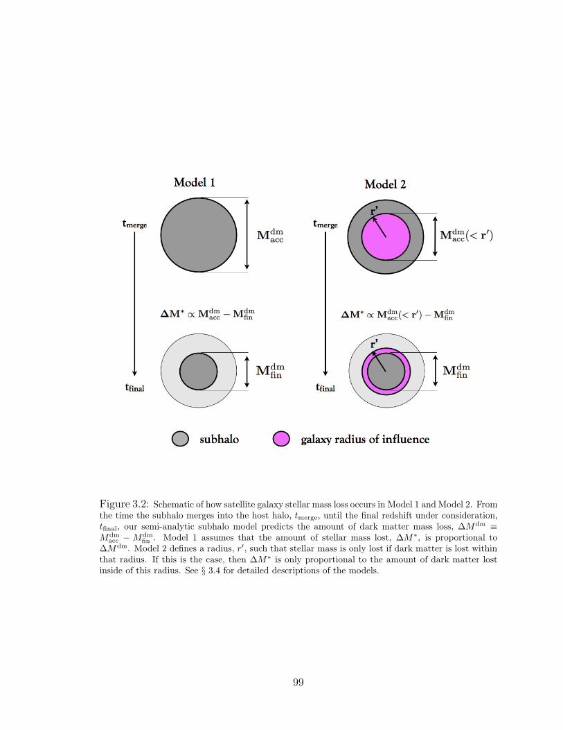
Figure 3.2: Schematic of how satellite galaxy stellar mass loss occurs in Model 1 and Model 2. Fromthe time the subhalo merges into the host halo, tmerge, until the final redshift under consideration,tfinal, our semi-analytic subhalo model predicts the amount of dark matter mass loss, ∆Mdm ≡Mdm

acc − Mdmfin . Model 1 assumes that the amount of stellar mass lost, ∆M∗, is proportional to

∆Mdm. Model 2 defines a radius, r′, such that stellar mass is only lost if dark matter is lost withinthat radius. If this is the case, then ∆M∗ is only proportional to the amount of dark matter lostinside of this radius. See § 3.4 for detailed descriptions of the models.

99

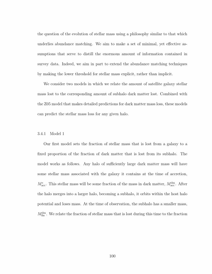
the question of the evolution of stellar mass using a philosophy similar to that which

underlies abundance matching. We aim to make a set of minimal, yet effective as-

sumptions that serve to distill the enormous amount of information contained in

survey data. Indeed, we aim in part to extend the abundance matching techniques

by making the lower threshold for stellar mass explicit, rather than implicit.

We consider two models in which we relate the amount of satellite galaxy stellar

mass lost to the corresponding amount of subhalo dark matter lost. Combined with

the Z05 model that makes detailed predictions for dark matter mass loss, these models

can predict the stellar mass loss for any given halo.

3.4.1 Model 1

Our first model sets the fraction of stellar mass that is lost from a galaxy to a

fixed proportion of the fraction of dark matter that is lost from its subhalo. The

model works as follows. Any halo of sufficiently large dark matter mass will have

some stellar mass associated with the galaxy it contains at the time of accretion,

M∗

acc. This stellar mass will be some fraction of the mass in dark matter, Mdmacc . After

the halo merges into a larger halo, becoming a subhalo, it orbits within the host halo

potential and loses mass. At the time of observation, the subhalo has a smaller mass,

Mdmfin . We relate the fraction of stellar mass that is lost during this time to the fraction

100

of dark matter mass that is lost through a single parameter ǫ,

∆M∗

M∗= ǫ

∆Mdm

Mdm, (3.2)

M∗

acc −M∗

fin

M∗acc

= ǫMdm

acc −Mdmfin

Mdmacc

, (3.3)

which can be re-written as,

M∗

fin = M∗

acc

[

1 − ǫ×(Mdm

acc −Mdmfin

Mdmacc

)

]

(3.4)

The left-hand side of Figure 3.2 is a cartoon schematic of how stellar mass loss

occurs in Model 1. From the time the subhalo merges into the host halo, tmerge, until

the final redshift under consideration, tfinal, the Z05 model (see § 3.3 for model details)

predicts the amount of subhalo dark matter mass loss ∆Mdm with the stellar mass

loss ∆M∗ being related to the dark matter mass loss via ǫ. Therefore, we are left

with a simple parametric equation governed by a single free parameter. For example,

if ǫ = 0.5, then a subhalo that loses 50% of its dark matter will lose 25% of its stellar

mass. As we mentioned above, stellar mass loss should be less efficient than dark

matter mass loss, so we should generally expect ǫ < 1.

In order to compute the final stellar mass of a galaxy via Eqn. 3.4, we need to know

the stellar mass of a satellite galaxy as a function of the subhalo mass at the time of

accretion. The stellar mass of a galaxy depends on many physical processes, including

mergers, gas cooling, star formation, feedback from supernovae, feedback from active

101

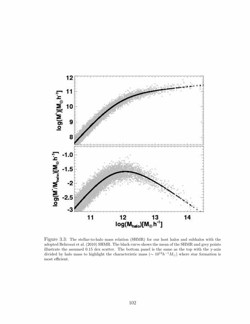
Figure 3.3: The stellar-to-halo mass relation (SHMR) for our host halos and subhalos with theadopted Behroozi et al. (2010) SHMR. The black curve shows the mean of the SHMR and grey pointsillustrate the assumed 0.15 dex scatter. The bottom panel is the same as the top with the y-axisdivided by halo mass to highlight the characteristic mass (∼ 1012h−1M⊙) where star formation ismost efficient.

102

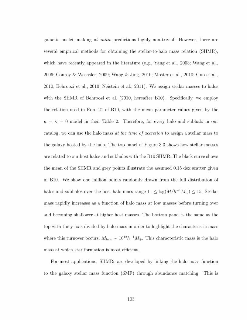
galactic nuclei, making ab initio predictions highly non-trivial. However, there are

several empirical methods for obtaining the stellar-to-halo mass relation (SHMR),

which have recently appeared in the literature (e.g., Yang et al., 2003; Wang et al.,

2006; Conroy & Wechsler, 2009; Wang & Jing, 2010; Moster et al., 2010; Guo et al.,

2010; Behroozi et al., 2010; Neistein et al., 2011). We assign stellar masses to halos

with the SHMR of Behroozi et al. (2010, hereafter B10). Specifically, we employ

the relation used in Eqn. 21 of B10, with the mean parameter values given by the

µ = κ = 0 model in their Table 2. Therefore, for every halo and subhalo in our

catalog, we can use the halo mass at the time of accretion to assign a stellar mass to

the galaxy hosted by the halo. The top panel of Figure 3.3 shows how stellar masses

are related to our host halos and subhalos with the B10 SHMR. The black curve shows

the mean of the SHMR and grey points illustrate the assumed 0.15 dex scatter given

in B10. We show one million points randomly drawn from the full distribution of

halos and subhalos over the host halo mass range 11 ≤ log(M/h−1M⊙) ≤ 15. Stellar

mass rapidly increases as a function of halo mass at low masses before turning over

and becoming shallower at higher host masses. The bottom panel is the same as the

top with the y-axis divided by halo mass in order to highlight the characteristic mass

where this turnover occurs, Mhalo ∼ 1012h−1M⊙. This characteristic mass is the halo

mass at which star formation is most efficient.

For most applications, SHMRs are developed by linking the halo mass function

to the galaxy stellar mass function (SMF) through abundance matching. This is

103

typically done using the subhalo mass at accretion which, by definition, presumes

that no stellar stripping occurs. However, even if stellar stripping occurs (i.e., if ǫ

is non-zero) we can still use a SHMR relation that assigns stellar mass at the time

the subhalo merges, due to the fact that the SMF is strongly dominated by central

galaxies. We emphasize that while there are many SHMRs in the literature, we are

not very sensitive to the particular choice of SHMR. As we will discuss in § 3.5, we

assign stellar masses to halos and subhalos and then rank them in stellar mass in order

to find the stellar mass cut-off (M∗

fin) that matches the observed number density of a

given galaxy luminosity threshold sample. Therefore, two SHMRs that yield the same

rank order for the halos and subhalos will be indistinguishable from each other, even

though the values of M∗

fin will be different (as well as the mass-to-light ratios). All

published SHMRs are monotonically increasing functions, so this behavior is general.

On the other hand, the scatter in the SHMR is important, as this will change the

rank order. We use the B10 scatter of 0.15 dex throughout our analysis, though we

test the effect of changing the scatter on our results in § 3.5.1. We also note that

we do not consider the fact that the stellar mass of a galaxy may actually increase

for some time after merging and becoming a satellite, as it has been recently shown

that star formation in active satellites may continue for several Gyr (see Wetzel et al.,

2011). Such detailed modeling is beyond the scope and intention of this work.

In summary, we take the following steps in Model 1 for assigning final stellar

masses to an ensemble of halos.

104

1. We use the Z05 model for subhalo evolution to obtain a list of halos and subhalos

for a range of host halo masses, and we determine the fractional amount of dark

matter mass lost from each subhalo.

2. We use the B10 stellar-to-halo mass relation to assign stellar masses to host

halos and subhalos at the time of accretion.

3. For every subhalo, we compute a final stellar mass by relating the fractional

amount of stellar mass lost to the fractional amount of dark matter mass lost

through the single free parameter ǫ, as described in Eqn. 3.4.

3.4.2 Model 2

Model 1 operates under the basic assumption that the fractional amount of satel-

lite galaxy stellar mass loss is proportional to subhalo dark matter loss through the

free parameter ǫ. This means that even a small amount of dark matter stripping will

be accompanied by some stellar stripping. However, as we argued in § 3.2, a sub-

halo may lose a considerable amount of dark matter before its galaxy is significantly

disturbed. For example, subhalos in high-resolution simulations lose a significant frac-

tion of mass at their outskirts rapidly upon merging into a larger system, while their

interiors remain unaltered by this mass loss (e.g., Diemand et al., 2007). Accordingly,

we consider an alternative model that incorporates a delay between the initial loss of

dark matter mass and stellar mass loss.

Our second model states that stellar mass will only be lost if a sufficient amount of

105

dark matter is lost first. The model works as follows. We first define an approximate

radius of influence that a galaxy has within its subhalo, corresponding to the region

within which the gravity due to the stellar component is comparable to that from

dark matter. To estimate this radius, we first assign a stellar mass to each subhalo at

the time of accretion, M∗

acc, using the B10 formalism. Next we assume, for simplicity,

that this is a point mass and we do not consider the total amount of “cold baryons”

or assume a galaxy profile. To find the radius of influence, rinfl, of the stellar mass

associated with the galaxy, we calculate where the dark matter mass enclosed within

the subhalo is equal to M∗

acc. We thus integrate the NFW mass profile,

Mdmacc (< rinfl) = 4πρ0r

3s

[

ln

(

1 +rinfl

rs

)

−rinfl/rs

1 + rinfl/rs

]

, (3.5)

where ρ0 and rs are the NFW parameters, and solve for rinfl by setting Mdmacc (< rinfl) =

M∗

acc.

The radius rinfl gives the rough scale within which mass must be lost before sig-

nificant stellar mass is lost; however, we allow for flexibility in this final prescription

for stellar mass loss. We assume that a galaxy will start losing stellar mass once dark

matter is stripped from inside a radius that scales linearly with rinfl. We define a

new radius, r′ = ψ × rinfl, where ψ is a free parameter of order unity. If the subhalo

loses so much dark matter that its final mass is less than Mdmacc (< r′), we allow stellar

stripping to occur. Furthermore, we assume that the fraction of stellar mass lost is

equal to the fraction of dark matter lost after the bound mass of the subhalo crosses

106

below this threshold. The final stellar mass of the galaxy is thus

M∗

fin = M∗

acc

[

1 − max

0,

(

Mdmacc (< r′) −Mdm

fin

Mdmacc (< r′)

)]

, (3.6)

which is analogous to Eqn. 3.4.

The right-hand side of Figure 3.2 illustrates how Model 2 works. After accretion,

if the subhalo shrinks enough due to mass loss such that its mass at the final redshift

of interest is less than Mdmacc (< r′), then stellar mass will be lost (∆M∗) in proportion

to the additional amount of dark matter lost. However, if mass loss does not reduce

the subhalo mass to less than Mdmacc (< r′), no stellar mass is lost. Model 2 incorporates

a delay between the stripping of the outer layers of dark matter and the stripping of

the stellar material residing in the depths of the subhalo potential well. The single

free parameter of Model 2, ψ, allows us to vary the amount of lag. As was the case

for ǫ = 0 in Model 1, setting ψ = 0 in Model 2 leads to zero stellar mass loss in all

subhalos.

In summary, we take the following steps in Model 2 for assigning final stellar

masses to an ensemble of halos.

1. We obtain a population of halos and assign stellar masses at the time of accretion

as described in the first two steps of the Model 1 summary.

2. For each subhalo, we calculate rinfl using Eqn. 3.5. We then scale this radius

using the free parameter ψ, to get r′ = ψ × rinfl.

107

3. We calculate the dark matter mass at accretion that is enclosed by r′, Mdmacc (<

r′). If insufficient dark matter loss has occurred, such that the final subhalo

mass is greater than this, then we assume that no stellar mass loss has taken

place. Otherwise, we estimate a final stellar mass using Eqn. 3.6.

3.5 Constraining Satellite Galaxy Stellar Mass Loss Using Galaxy Clustering

We now turn to constraints on the relationship between stellar mass and halo

mass imposed by the clustering of galaxies. Our two stellar mass loss models specify

the final stellar mass in any halo or subhalo, given a value for the parameter ǫ (for

Model 1) or ψ (for Model 2). With stellar masses assigned to all halos and subhalos,

we can predict a halo occupation distribution (HOD: e.g., Peacock & Smith, 2000;

Scoccimarro et al., 2001; Berlind & Weinberg, 2002; Cooray & Sheth, 2002) for any

given stellar mass threshold. In particular, we compute the mean number of galaxies

as a function of host halo mass, 〈N〉M. We calculate the mean over the 500 host halo

realizations at each host mass. We use this function to compute the number density

of galaxies by weighting the host halo abundances by 〈N〉M and integrating over all

halo masses,

ng =

∫

∞

0

dMdn

dM〈N〉M . (3.7)

We adopt the Warren et al. (2006) halo mass function, dn/dM , in this calculation,

though our results are not sensitive to the specific choice of mass function. In this

way, we find the stellar mass threshold that yields a galaxy number density equal to

108

that of the observed sample with which we aim to compare.

We compare our model predictions to four of the Sloan Digital Sky Survey (SDSS:

York et al., 2000) luminosity threshold galaxy samples measured by Zehavi et al.

(2011). Specifically, we consider volume-limited samples with r-band absolute mag-

nitude thresholds of Mr ≤ −18, −19, −20, and −21 (number densities for these

samples are listed in Table 2 of Zehavi et al. 2011). We do not consider the fact that

the observed relationship between stellar mass and luminosity is not one-to-one (i.e.,

galaxies of a fixed luminosity can have different stellar masses which, for instance, is

manifested as scatter in the Tully-Fisher relation – Bell & de Jong 2001). However,

including this scatter should be similar to increasing the scatter in the B10 relation

between dark matter mass and M∗

acc, which has a very small effect, as we show in

§ 3.5.1.

Once we have determined the appropriate stellar mass threshold, we use the re-

sulting HOD to calculate the predicted clustering of the model. We place galaxies

within the host halos in a N-body simulation to measure the 2PCF. We use a single

realization of the “Consuelo” simulation (with a box size of 420h−1Mpc and 14003

particles), which is part of the LasDamas suite of simulations (McBride et al., in

prep.). The cosmology assumed in our semi-analytic subhalo model is set to match

that of the LasDamas simulations3 and is similar to the recent WMAP7 values (Ko-

3Throughout the paper, we work within the standard, vacuum-dominated, cold dark matter(ΛCDM) cosmological model with Ωm = 0.25, ΩΛ = 0.75, Ωb = 0.04, h0 = 0.7, σ8 = 0.8, andns = 1.0.

109

matsu et al., 2011). We use the spherical over-density (SO) halo finder “Rockstar”

(Behroozi et al., 2011) to identify halos. We use an SO halo finder because the SO

algorithm mimics the assumptions made in our semi-analytic model. Both the Z05

model and the halo finder define virial masses based on the virial threshold definition

of Bryan & Norman (1998). We note, however, that our results are not sensitive to the

choice of halo finder. We have repeated our analysis using a Friends-of-Friends halo

finder and derived similar results. We populate host halos with galaxies according to

our 〈N〉M model predictions.

In order to compare to data, we convert our real-space correlation functions, ξ(r),

to projected correlation functions, wp(rp), by integrating along lines of sight (Davis &

Peebles, 1983; Zehavi et al., 2004):

wp(rp) = 2

∫ ymax

0

ξ(√

r2p + y2

)

dy. (3.8)

For each luminosity threshold, we integrate out to the same ymax as Zehavi et al.

(2011, listed as πmax in their Table 2). We predict wp(rp) for the four luminosity

samples, given any value of ǫ from Model 1 or ψ from Model 2. In order to constrain

our stellar mass loss models, we run a grid of ǫ and ψ values in steps of ∆ǫ = 0.1 and

∆ψ = 0.05. For each parameter value and each luminosity threshold, we compute

χ2 by comparing our model prediction to the Zehavi et al. (2011) measurement of

wp(rp), using only diagonal errors (not the full covariance matrices).

Figure 3.4 shows clustering results for Model 1 compared to measurements from

110

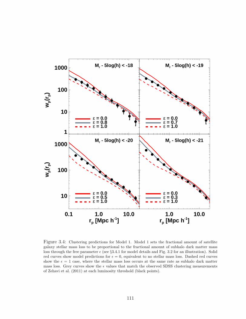
1

10

100

1000

wp(r

p)

ε = 1.0ε = 0.8ε = 0.0

Mr - 5log(h) < -18

Mr - 5log(h) < -19

ε = 1.0ε = 0.7ε = 0.0

0.1 1.0 10.0rp [Mpc h-1]

10

100

1000

wp(r

p)

Mr - 5log(h) < -20

ε = 1.0ε = 0.5ε = 0.0

1.0 10.0rp [Mpc h-1]

Mr - 5log(h) < -21

ε = 1.0ε = 0.3ε = 0.0

Figure 3.4: Clustering predictions for Model 1. Model 1 sets the fractional amount of satellitegalaxy stellar mass loss to be proportional to the fractional amount of subhalo dark matter massloss through the free parameter ǫ (see §3.4.1 for model details and Fig. 3.2 for an illustration). Solidred curves show model predictions for ǫ = 0, equivalent to no stellar mass loss. Dashed red curvesshow the ǫ = 1 case, where the stellar mass loss occurs at the same rate as subhalo dark mattermass loss. Grey curves show the ǫ values that match the observed SDSS clustering measurementsof Zehavi et al. (2011) at each luminosity threshold (black points).

111

Zehavi et al. (2011) for our four SDSS luminosity threshold samples: Mr < −18,−19,−20 and −

21. To reiterate, Model 1 assumes that the fractional amount of satellite galaxy stellar

mass loss is proportional to the fractional amount of subhalo dark matter mass loss

with proportionality constant ǫ. Adopting ǫ = 0 specifies no stellar mass loss and is

equivalent to using Vmax at the epoch of accretion for abundance matching. On the

other hand, adopting ǫ = 1 means that stellar mass is lost at the same rate as dark

matter. For each luminosity sample, we show the ǫ = 0 and 1 cases as red solid and

dashed lines, respectively.

At each luminosity, ǫ = 0 predicts small-scale clustering that is stronger than the

data indicate and this gets to the essence of using clustering to constrain stellar mass

loss. This over-prediction can be attributed to the fact that no stellar mass loss has

occurred for satellite galaxies, resulting in too many satellites with high stellar masses.

This leads to enhanced clustering on small scales (e.g. Watson et al., 2011b). To be

consistent with the data, some stellar mass loss needs to occur. However, the ǫ = 1

result demonstrates that too much stellar mass loss leads to weaker clustering than

the data require. The grey curves in Figure 3.4 correspond to intermediate amounts

of stellar mass loss and represent the ǫ with the lowest χ2 values.4 Despite the fact

that Model 1 paints a simplified picture of how stars are stripped from the galaxies

they reside in, we show that it is very effective at matching the observed clustering.

4We note that none of our model predictions match the large-scale clustering for the Mr < −18sample. This may be attributed to the finite volume of the sample, as discussed in § 3.2 of Zehaviet al. (2011).

112

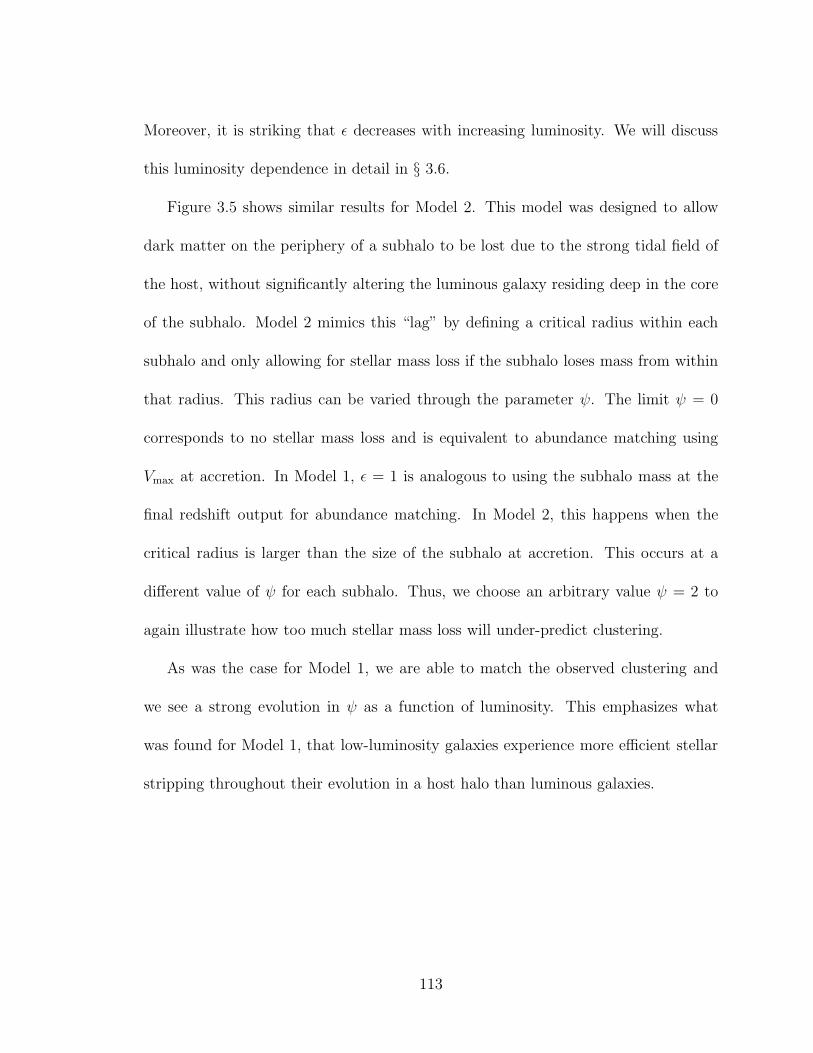
Moreover, it is striking that ǫ decreases with increasing luminosity. We will discuss

this luminosity dependence in detail in § 3.6.

Figure 3.5 shows similar results for Model 2. This model was designed to allow

dark matter on the periphery of a subhalo to be lost due to the strong tidal field of

the host, without significantly altering the luminous galaxy residing deep in the core

of the subhalo. Model 2 mimics this “lag” by defining a critical radius within each

subhalo and only allowing for stellar mass loss if the subhalo loses mass from within

that radius. This radius can be varied through the parameter ψ. The limit ψ = 0

corresponds to no stellar mass loss and is equivalent to abundance matching using

Vmax at accretion. In Model 1, ǫ = 1 is analogous to using the subhalo mass at the

final redshift output for abundance matching. In Model 2, this happens when the

critical radius is larger than the size of the subhalo at accretion. This occurs at a

different value of ψ for each subhalo. Thus, we choose an arbitrary value ψ = 2 to

again illustrate how too much stellar mass loss will under-predict clustering.

As was the case for Model 1, we are able to match the observed clustering and

we see a strong evolution in ψ as a function of luminosity. This emphasizes what

was found for Model 1, that low-luminosity galaxies experience more efficient stellar

stripping throughout their evolution in a host halo than luminous galaxies.

113

1

10

100

1000

wp(r

p)

ψ = 2.0ψ = 0.95ψ = 0.0

Mr - 5log(h) < -18

Mr - 5log(h) < -19 Mr - 5log(h) < -19

ψ = 2.0ψ = 0.7ψ = 0.0

0.1 1.0 10.0rp [Mpc h-1]

10

100

1000

wp(r

p)

Mr - 5log(h) < -20

ψ = 2.0ψ = 0.4ψ = 0.0

1.0 10.0rp [Mpc h-1]

Mr - 5log(h) < -21

ψ = 2.0ψ = 0.35ψ = 0.0

Figure 3.5: Clustering results for Model 2. Model 2 defines a radius of influence, rinfl, for a galaxywithin a subhalo. If a subhalo loses sufficient dark matter mass such that it starts to lose massinside of rinfl, then stellar mass is lost at a rate proportional to the subsequent subhalo mass loss.The free parameter ψ allows rinfl to grow or shrink, thus a larger value of ψ means that more stellarmass loss will occur on average for satellite galaxies. Solid red curves show model predictions forψ = 0, equivalent to no stellar mass loss, thus the same as ǫ = 0 for Model 1. Dashed red curvesshow the predictions for ψ = 2, an arbitrary value chosen to represent how too much stellar massloss will under-predict wp(rp). Grey curves show the ψ values that match the observed clusteringfor the same luminosity threshold samples as in Fig. 3.4.

114

3.5.1 The Effect of Scatter in the Stellar-to-Halo Mass Relation

Observations indicate that halos of a given mass can host galaxies with a range of

luminosities and stellar masses (e.g., van den Bosch et al., 2007; Zheng et al., 2007;

Yang et al., 2008; More et al., 2009). For this reason, it is overly restrictive to assume

a one-to-one relation between halo mass and stellar mass, whereas a relationship

with some intrinsic scatter is more appropriate. This is especially true for abundance

matching because the presence of scatter changes the rank order of galaxies. We

rank our halos and subhalos by stellar mass, so the rank order will be affected by

the assumed amount of scatter. Scatter is typically accounted for by assuming a

distribution of stellar mass at fixed halo mass, with the mean value of stellar mass

given by a particular SHMR. For example, the B10 scatter that we adopt in this

paper is a log-normal distribution with a dispersion σ = 0.15. We implement this

scatter by randomly drawing from this distribution when we assign stellar masses to

halos and subhalos at the time of accretion. The results shown in Figures 3.4 and 3.5

include this scatter.

We repeat our analysis with different dispersions in order to test the sensitivity

of our results to uncertainty of the scatter in the SHMR. Figure 3.6 Shows the effect

of changing the SHMR dispersion for one of the models that matches the clustering

of Mr < −21 galaxies: Model 1 with ǫ = 0.3. This sample is the most sensitive to

scatter because the slope of the SHMR is shallowest for luminous galaxies and thus

a given amount of scatter in stellar mass at fixed halo mass translates into a large

115

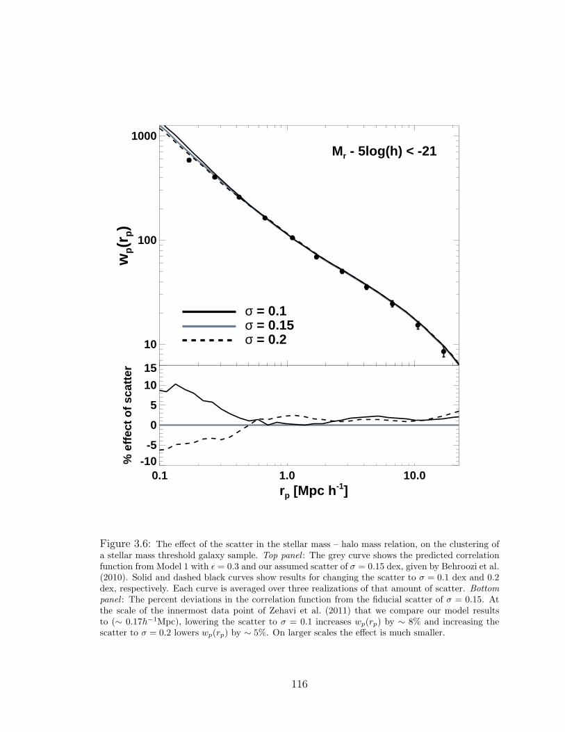
10

100

1000w

p(r

p)

rp [Mpc h-1]

σ = 0.2σ = 0.15σ = 0.1

Mr - 5log(h) < -21

0.1 1.0 10.0-10-5

0

5

10

15

% e

ffec

t o

f sc

atte

r

Figure 3.6: The effect of the scatter in the stellar mass – halo mass relation, on the clustering ofa stellar mass threshold galaxy sample. Top panel : The grey curve shows the predicted correlationfunction from Model 1 with ǫ = 0.3 and our assumed scatter of σ = 0.15 dex, given by Behroozi et al.(2010). Solid and dashed black curves show results for changing the scatter to σ = 0.1 dex and 0.2dex, respectively. Each curve is averaged over three realizations of that amount of scatter. Bottom

panel : The percent deviations in the correlation function from the fiducial scatter of σ = 0.15. Atthe scale of the innermost data point of Zehavi et al. (2011) that we compare our model resultsto (∼ 0.17h−1Mpc), lowering the scatter to σ = 0.1 increases wp(rp) by ∼ 8% and increasing thescatter to σ = 0.2 lowers wp(rp) by ∼ 5%. On larger scales the effect is much smaller.

116

scatter in halo mass at a fixed stellar mass threshold (see Fig. 3.3). The top panel of

Figure 3.6 shows the correlation function for three SHMR dispersions: σ = 0.1, 0.15,

and 0.2. The bottom panel depicts percent deviations from the fiducial scatter of

σ = 0.15. This range is conservative, as it is larger than the errors in scatter quoted

in B10 (especially at the low end). The figure demonstrates that changing the scatter

has a small effect on wp(rp), in the sense that more scatter generally leads to a lower

amplitude of clustering on small scales. Over the range of data points from the Zehavi

et al. (2011) data that we model, there is a maximum ∼ 8% and ∼ 5% shift in wp(rp)

for the σ = 0.1 and σ = 0.2 cases, respectively. This is not a large effect and does

not result in a significant change to the best-fit values of ǫ or ψ. Uncertainties in the

scatter of the SHMR do not significantly alter our results or our primary conclusions.

3.6 Luminosity Dependence of Satellite Galaxy Stellar Mass Loss

Figures 3.4 & 3.5 indicate that the best-fit values of both ǫ and ψ vary with

luminosity. We highlight these trends in Figure 3.7. The left-hand panel summarizes

results from Model 1, and demonstrates that the best-fit value of ǫ drops from ǫ = 0.8

for Mr < −18 galaxies to ǫ = 0.3 for Mr < −21 galaxies. There is a strong luminosity

dependence associated with satellite galaxy stellar mass loss, such that relatively low-

luminosity satellite galaxies lose more stellar material per unit of dark matter than

more luminous satellite galaxies. The right-hand panel of Figure 3.7 summarizes

results from Model 2, which show a consistent trend. The best-fit value of ψ drops

117

Model 1

-18 -19 -20 -21Mr

0.0

0.2

0.4

0.6

0.8

1.0

ε

Model 2

-18 -19 -20 -21Mr

0.0

0.2

0.4

0.6

0.8

1.0

ψ

Figure 3.7: The luminosity dependence of satellite galaxy stellar mass loss. Left panel : The best-fit Model 1 parameter ǫ as a function of absolute r-band magnitude. The decreasing trend of ǫ withincreasing luminosity means that low-luminosity satellite galaxies experience greater stellar mass lossrelative to subhalo dark matter mass loss than luminous galaxies. Right panel : The best-fit Model 2parameter ψ as a function of absolute r-band magnitude. The decreasing trend of ψ with increasingluminosity means that low-luminosity satellite galaxies have a greater radius of influence (causingmore stellar mass loss) than luminous galaxies. In other words, the same qualitative luminositytrend is seen in both models.

from ψ = 0.95 for Mr < −18 galaxies to ψ = 0.35 for Mr < −21 galaxies. Lower

values of ψ indicate less stellar mass loss for a given amount of dark matter mass loss.

The two models we explore absorb a significant number of subtle effects into simple

assumptions. Model 1 and Model 2 differ substantially in detail, yet both analyses

indicate that the luminosity dependence of galaxy clustering can be explained if low-

luminosity satellite galaxies lose stars more efficiently than luminous galaxies.

What does this result mean? Presumably it means that the stars within luminous

galaxies are more tightly bound – relative to their surrounding dark matter – than

the stars in less luminous galaxies. This could be due to luminous galaxies having

more compact stellar density profiles. In fact, it may be that this result can be ex-

118

plained by the well-known correlation between galaxy luminosity and morphology,

whereby luminous galaxies are more likely to be ellipticals than low-luminosity galax-

ies. For example, Blanton et al. (2003) showed that the mean Sercic index of galaxies

roughly doubles from Mr = −18 to Mr = −21 (looking at their Fig. 9 and con-

verting i-band to r-band magnitudes). We must, of course, keep in mind that these

morphology-luminosity correlations apply to all galaxies, of which satellites are only

a small portion. It may be that these correlations would vanish in samples containing

only satellite galaxies.

An ancillary consideration is the relative size of galaxies compared to the typical

(sub)halos they occupy. For instance, using a sample of 140,000 SDSS galaxies, Shen

et al. (2003) showed the size distribution (half-light radii) of early- and late-type

galaxies as a function of r-band luminosity and stellar mass. Examining their Figs. 2

& 3, the half-light radius R increases roughly by a factor of ∼ 3 from Mr < −19.25

to −22.25 for late-type galaxies, and by a factor of ∼ 5 for early types. However,

if we consider the typical halo masses that host these galaxies (see Mmin values for

Mr < −19 and −22 from Table 3 of Zehavi et al. 2011), they correspond to virial

radii of ∼ 125h−1kpc and ∼ 750h−1kpc, respectively, a factor of 6. In other words, at

a very approximate level, larger (more luminous) galaxies are slightly deeper within

their host halo potential wells than smaller (less luminous) galaxies, and are relatively

less susceptible to stellar stripping.

The luminosity trend that we have found demonstrates the power of our modeling

119

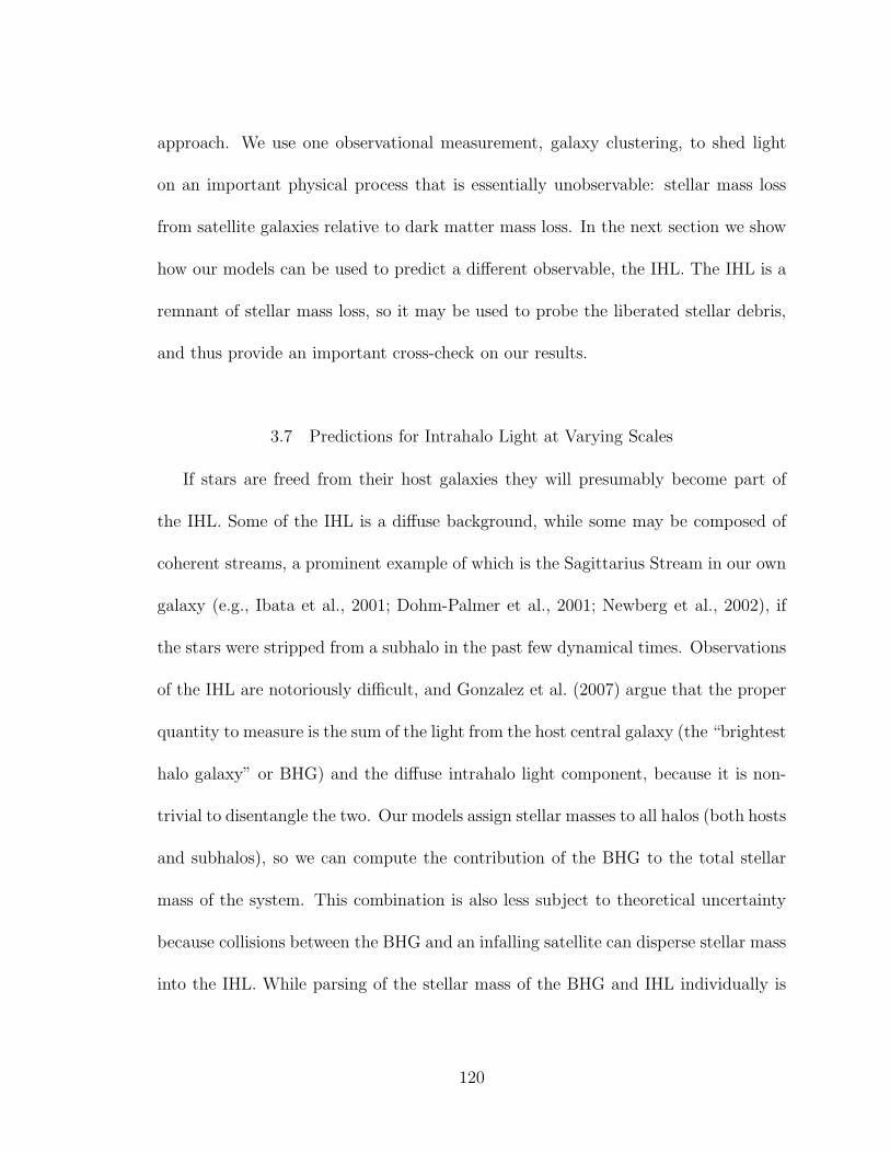
approach. We use one observational measurement, galaxy clustering, to shed light

on an important physical process that is essentially unobservable: stellar mass loss

from satellite galaxies relative to dark matter mass loss. In the next section we show

how our models can be used to predict a different observable, the IHL. The IHL is a

remnant of stellar mass loss, so it may be used to probe the liberated stellar debris,

and thus provide an important cross-check on our results.

3.7 Predictions for Intrahalo Light at Varying Scales

If stars are freed from their host galaxies they will presumably become part of

the IHL. Some of the IHL is a diffuse background, while some may be composed of

coherent streams, a prominent example of which is the Sagittarius Stream in our own

galaxy (e.g., Ibata et al., 2001; Dohm-Palmer et al., 2001; Newberg et al., 2002), if

the stars were stripped from a subhalo in the past few dynamical times. Observations

of the IHL are notoriously difficult, and Gonzalez et al. (2007) argue that the proper

quantity to measure is the sum of the light from the host central galaxy (the “brightest

halo galaxy” or BHG) and the diffuse intrahalo light component, because it is non-

trivial to disentangle the two. Our models assign stellar masses to all halos (both hosts

and subhalos), so we can compute the contribution of the BHG to the total stellar

mass of the system. This combination is also less subject to theoretical uncertainty

because collisions between the BHG and an infalling satellite can disperse stellar mass

into the IHL. While parsing of the stellar mass of the BHG and IHL individually is

120

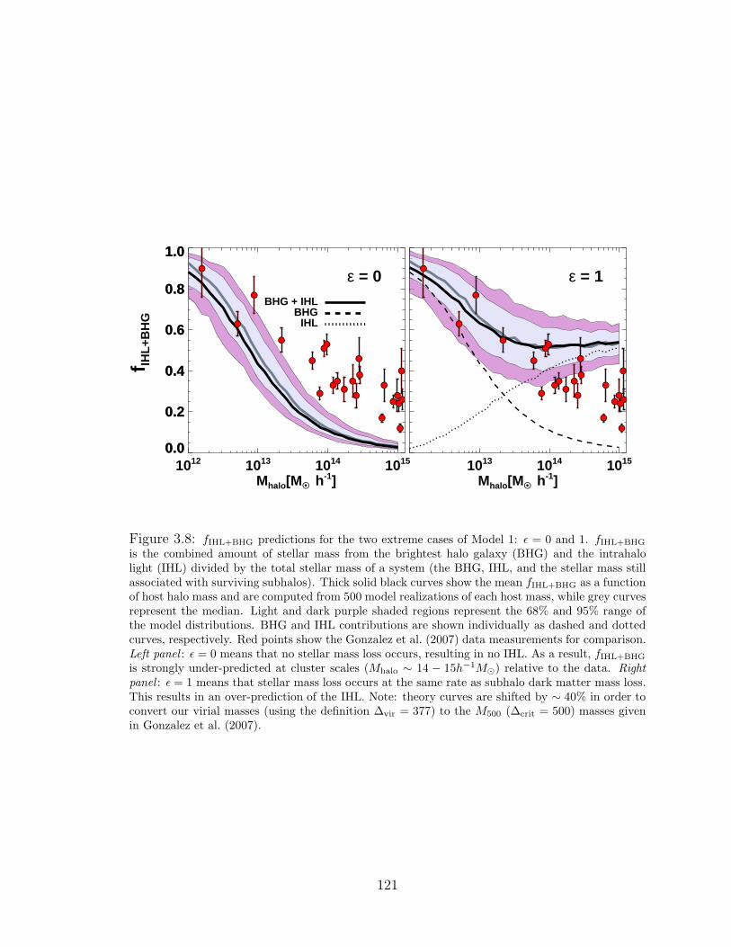
1012 1013 1014 1015

Mhalo[MO • h-1]

0.0

0.2

0.4

0.6

0.8

1.0

f IHL

+BH

G

ε = 0BHG + IHL

BHGIHL

0.0

0.2

0.4

0.6

0.8

1.0

1013 1014 1015

Mhalo[MO • h-1]

ε = 1

Figure 3.8: fIHL+BHG predictions for the two extreme cases of Model 1: ǫ = 0 and 1. fIHL+BHG

is the combined amount of stellar mass from the brightest halo galaxy (BHG) and the intrahalolight (IHL) divided by the total stellar mass of a system (the BHG, IHL, and the stellar mass stillassociated with surviving subhalos). Thick solid black curves show the mean fIHL+BHG as a functionof host halo mass and are computed from 500 model realizations of each host mass, while grey curvesrepresent the median. Light and dark purple shaded regions represent the 68% and 95% range ofthe model distributions. BHG and IHL contributions are shown individually as dashed and dottedcurves, respectively. Red points show the Gonzalez et al. (2007) data measurements for comparison.Left panel : ǫ = 0 means that no stellar mass loss occurs, resulting in no IHL. As a result, fIHL+BHG

is strongly under-predicted at cluster scales (Mhalo ∼ 14 − 15h−1M⊙) relative to the data. Right

panel : ǫ = 1 means that stellar mass loss occurs at the same rate as subhalo dark matter mass loss.This results in an over-prediction of the IHL. Note: theory curves are shifted by ∼ 40% in order toconvert our virial masses (using the definition ∆vir = 377) to the M500 (∆crit = 500) masses givenin Gonzalez et al. (2007).

121

sensitive to the fraction of stellar mass ejected in such collisions, the sum is robust to

uncertainties in this process.

We start by investigating the predictions for the ǫ = 0 and ǫ = 1 cases from

Model 1. These extremes were shown in § 3.5 to over- and under-predict the observed

clustering, respectively, for each luminosity threshold. In Figure 3.8, we show the

fraction of the total stellar mass of a system (including stellar mass in satellite galax-

ies), that is contained within both the IHL and the BHG, fIHL+BHG, as a function

of host halo mass, Mhalo. The thick solid black curves in Figure 3.8 show the mean

value of fIHL+BHG obtained from our 500 realizations of host halos, and grey curves

represent the median. The inner and outer shaded regions represent the 68% and 95%

ranges of the model distributions. The mean individual BHG and IHL contributions

are shown distinctly as dashed and dotted curves, respectively. The fIHL+BHG data

from Gonzalez et al. (2007) are shown as red circles with errorbars, and are the same

in both panels.

For ǫ = 0 there is no stellar mass loss, and thus no contribution to the total stellar

mass of the system from the IHL. The stellar mass of the BHG alone provides a decent

description of the data for halo masses below group mass scales, Mhalo . 1013 h−1M⊙.

While less massive systems have been observed to have some detectable IHL (see

§ 5.1), it is mainly large group- and cluster-size objects that are known to have

significant IHL components. It is therefore not surprising that the ǫ = 0 model

underestimates fIHL+BHG on these scales.

122

At the other extreme, the ǫ = 1 model assumes that stellar mass is lost with the

same efficiency as dark matter. We argued in § 3.4 that this over-estimates stellar

mass loss, so it is not surprising that choosing ǫ = 1 leads to an overestimate of

fIHL+BHG for systems greater than large groups (Mhalo & 1013.5 h−1M⊙). At lower

masses, typical infalling satellites have halo masses below Mdmacc . 1011 h−1M⊙ and

bring with them only a small amount of stellar mass (B10). This is the regime of the

SHMR where stellar mass rapidly decreases with decreasing halo mass (see Fig. 3.3).

Data are not yet precise enough to be sensitive to the stellar mass carried into the

systems by such small, infalling subhalos. Consequently, fIHL+BHG ≈ fBHG and can

be adequately described in low-mass systems at both the ǫ = 1 and ǫ = 0 extremes.

We note that in our model predictions for the IHL, we only consider the stellar

mass stripped from satellite galaxies that have stellar masses equivalent to Mr < −18

galaxies and brighter. We ignore stellar mass loss from less luminous (less massive)

satellites in the fIHL+BHG calculation. However, the stellar mass locked up in these

lower mass “uncounted” subhalos only amounts to ∼ 3% of the total stellar mass

within a given host halo, so neglecting them has a negligible effect on our fIHL+BHG

model predictions. We also note that in Figure 3.8 we have shifted the data points

to higher masses by ∼ 40% in order to convert the M500 (∆crit = 500) masses given

in Gonzalez et al. (2007) to our virial masses (using the definition ∆vir = 377). We

assumed an NFW profile to perform this conversion.

Having shown that these two extreme cases are not able to describe the data

123

1012 1013 1014 1015

Mhalo[MO • h-1]

0.0

0.2

0.4

0.6

0.8

1.0

f IHL

+BH

G

Model 1

BHG + IHLBHG

IHL

0.0

0.2

0.4

0.6

0.8

1.0

1013 1014 1015

Mhalo[MO • h-1]

Model 2

Figure 3.9: fIHL+BHG predictions for our best-fit Model 1 (left panel) and Model 2 (right panel).We compute each subhalo’s contribution to the IHL according to its initial stellar mass by using theappropriate best-fit values of ǫ or ψ. For example, a subhalo with a stellar mass that correspondsto a galaxy of absolute r-band magnitude equal to -18.5 loses stellar mass according to ǫ = 0.8(in Model 1), whereas a subhalo with a stellar mass corresponding to Mr = −20.5 loses stellarmass according to ǫ = 0.5. Shaded regions, curves, and points are as in Fig. 3.8. Our stellarmass loss models predict that the mean IHL fraction in halos increases from a few percent atthe scale of individual galaxies (Mhalo ∼ 1012h−1M⊙) to ∼ 20 − 25% at cluster scales (Mhalo ∼1014 − 1015h−1M⊙). Both models succeed in matching the mean trend observed by Gonzalez et al.(2007). However, Model 1 seems to under-predict the scatter in fIHL+BHG, whereas Model 2 predictsa scatter that is more consistent with the data measurements. We thus find that this more physically-motivated model for satellite galaxy stellar mass loss is favored over Model 1.

124

accurately, we turn to the predictions of our models. To make fIHL+BHG predictions

at a given host halo mass scale we need to assign each (sub)halo an ǫ value for Model 1

and a ψ value for Model 2. Let us examine just the Model 1 case for simplicity. When

we found the best-fit value of ǫ for each luminosity threshold sample in § 3.5, we also

determined a final stellar mass threshold for the sample through abundance matching.

For example, the Mr < −20 sample was found to correspond to halos and subhalos

with final stellar masses greater than some value M∗

fin,20, where final stellar masses

are predicted using ǫ = 0.5. The Mr < −21 sample corresponds to stellar masses

greater than M∗

fin,21, where final stellar masses are predicted using ǫ = 0.3, and so on.

We assign each subhalo a value of ǫ using these stellar mass thresholds. For example,

if a subhalo has a stellar mass at accretion that falls between M∗

fin,20 and M∗

fin,21, we

assign it ǫ = 0.5. If, instead, it has a mass between M∗

fin,19 and M∗

fin,20, we assign

it ǫ = 0.7. It is awkward to use the stellar mass at accretion to assign subhalos to

ranges in M∗

fin, but we cannot estimate final stellar masses without having a value of

ǫ in the first place, so we are stuck with this approximate method. We follow the

same process for Model 2 by choosing the appropriate ψ values. We emphasize that

these ǫ and ψ values are not “tuned” to agree with the fIHL+BHG observations, rather

are genuine predictions that result from parameter values found from matching to

clustering data.

Figure 3.9 shows the Model 1 (left panel) and Model 2 (right panel) fIHL+BHG

predictions, as well as the individual IHL and BHG contributions. While fIHL+BHG

125

rapidly decreases with increasing host halo mass, the contribution to fIHL+BHG from

the IHL increases. This supports a picture in which galaxy-mass halos have very few

luminous satellite galaxies and little IHL, so the stellar masses of these systems are

dominated by the BHGs. Galaxy size halos accrete the majority of their mass from

small subhalos that have very high mass-to-light ratios (Purcell et al., 2007). There-

fore, shredded satellites deposit very little stellar mass into the IHL. The number of

large satellites increases with host halo mass. The larger and more common subhalos

within larger host halos may form stars more efficiently (have lower mass-to-light ra-

tios) and provide a source for developing significant IHL. Both models find that host

masses of Mhost/h−1M⊙ = 1012, 1013, 1014, and 1015, contain mean IHL fractions of

fIHL ∼ 2%, 10%, 20%, and 25%, respectively. This is in good agreement with several

previous studies, as we discuss in § 3.8. The IHL thus provides an independent check

of our stellar mass loss results.

Figure 3.9 contains a comparison between our model predictions and the Gonzalez

et al. (2007) data. Both models predict mean fIHL+BHG fractions that are consistent

with the observations.5 Interestingly, we find that the scatter predicted by Model 1

is substantially smaller than it is for Model 2 and it appears to be inconsistent with

the scatter found by Gonzalez et al. (2007). On the other hand, Model 2 is more

successful in reproducing the observed scatter in fIHL+BHG. To quantify this, we

5We note that this discussion assumes that the Gonzalez et al. (2007) data are accurate, whereasthey may be systematically overestimated due to an assumed constant mass-to-light ratio (Leauthaudet al., 2011).

126

calculate the probability that the scatter in the Gonzalez et al. (2007) data points

could result from the model distributions. We do this as follows. First, we restrict

the comparison to the high mass regime (the last 8 data points) because we wish to

investigate the scatter at fixed mass (if we include lower mass points, the measured

scatter will be affected by the mean trend of fIHL+BHG vs. mass). We next create

a model data set by choosing a single model realization of a host halo (out of the

500) for each Gonzalez et al. (2007) data point, at the appropriate halo masses. This

leads to 8 model values of fIHL+BHG. We then add a Gaussian random error to these

values, using the corresponding Gonzalez et al. (2007) errorbars. To fully sample

the distribution of data sets that could arise from our models, we repeat this process

10,000 times. Finally, we measure the weighted standard deviation of fIHL+BHG values

for the observed data, as well as each of the 10,000 model data sets. We find that

in Model 1, only 0.8% of the model data sets have a scatter that exceeds that of the

Gonzalez et al. (2007) data, whereas in Model 2, 25% of the model data sets have a

larger scatter.

This statistical test indicates that Model 1 should be rejected (at the 2.7σ level)

in favor of Model 2, an indication that is not entirely surprising given that Model 2

accounts for delayed stellar mass loss that is to be expected on physical grounds.

Model 1 assumes that stellar mass loss is simply proportional to subhalo mass loss,

so the scatter predicted by this model must be primarily caused by the scatter in the

total amount of dark matter mass loss, with a secondary amount of scatter coming

127

from the stellar to halo mass relation. On the other hand, Model 2 allows for greater

variation in the amount of stellar mass loss. For example, let us suppose two subhalos

start with the same mass at accretion and lose the same amount of dark matter. Now

let us suppose one contains 10% more stellar mass at accretion due to the scatter in

the SHMR. According to Model 1, both galaxies will lose the same fraction of their

stellar mass and so the one galaxy will inject 10% more stars into the IHL. According

to Model 2, however, the actual fraction of stars lost depends on stellar mass through

the galaxy’s radius of influence. The more massive galaxy will lose a higher fraction

of its stellar mass, thus causing a larger than 10% discrepancy in the total stellar

mass lost between the two galaxies.

3.8 Summary & Discussion

While galaxy formation is complex, we have shown in this paper that an un-

derstanding of the fates of satellite galaxies provides key insight into the galaxy

formation puzzle. Satellite galaxies live extremely tumultuous lives. Their spatial

clustering can shed light on how they lose stellar mass and contribute to building the

IHL over a large range of host halo mass scales. Part of our motivation for using

galaxy clustering to constrain stellar mass loss stems from possible shortcomings in

the commonly-employed abundance matching technique (e.g., Wetzel & White, 2010;

Yang et al., 2011, Reddick et al., in prep.), which suggest natural generalizations with

the gross form of the particular models we study. The standard method of abundance

128

matching involves mapping galaxies to halos by assuming a relationship between halo

(and subhalo) mass (or circular velocity) and a galaxy property (luminosity or stellar

mass) at a particular time. A galaxy luminosity assignment according to halo mass

at the time the halo was first accreted onto a larger system provides a very useful

description of known galaxy clustering properties (e.g., Conroy et al., 2006). How-

ever, this type of assignment implies that no stellar mass loss will occur. This is

contrary to many aspects of galaxy, group, and cluster evolution, including the pre-

vailing paradigm in which the IHL is produced by stellar mass liberated from infalling

galaxies by interactions in the group environment (e.g., Conroy et al., 2007; Purcell

et al., 2007). Abundance matching is also sensitive to the resolution of the cosmo-

logical simulation on which it is implemented. Subhalos are artificially destroyed by

falling below the numerical resolution limit and immediately removed from the galaxy

population irrespective of their circular velocities at their accretion times. This can

lead to differing predictions for the small-scale clustering of galaxies of a particular

luminosity among simulations with a fixed mapping of halo size onto luminosity.

These considerations persuaded us to explore simple models that associate stellar

masses to subhalo masses and constrain satellite galaxy stellar mass loss by match-

ing to clustering data. We implemented two distinct models. Model 1 related the

fractional amount of stellar mass loss to that of the subhalo dark matter mass loss

from the time of accretion until the final redshift through a single free parameter ǫ.

Model 2 was introduced to mimic a “lag” in stellar mass loss wherein the satellite

129

galaxy at the core of the subhalo experiences no stellar mass loss until the subhalo

has been stripped of sufficient dark matter on its periphery. Stellar mass loss in this

model only occurs once dark matter has been lost interior to a radius of influence

of the satellite galaxy. We introduced the free parameter ψ that dictated how the

radius of influence could expand or shrink allowing for more or less stellar mass loss.

We calculated the values of ǫ and ψ that matched the observed clustering of SDSS

galaxies over a large range of luminosity threshold samples. Matching to the observed

clustering at each luminosity threshold directly informs us of the amount of stellar

mass lost from satellite galaxies and, thus, will comprise the IHL.

This procedure enables predictions for the amount of IHL or IHL+BHG compared

to the total stellar mass of a host system of a given mass (fIHL and fIHL+BHG, respec-

tively). Observationally, it has been established that the amount of diffuse material

is nearly negligible at the scale of individual galaxies (e.g., Sackett et al., 1994; Mor-

rison et al., 1997; Weil et al., 1997; Lequeux et al., 1998; Abe et al., 1999; Zibetti &

Ferguson, 2004; Bailin et al., 2011). For example, M33, which is ∼ 1011 M⊙, has been

estimated to have an fIHL ≤ 1% (McConnachie et al., 2006; Hood et al., 2007). Our

own Milky Way is thought to have an fIHL ∼ 1% (e.g., Morrison, 1993; Wetterer &

McGraw, 1996; Chiba & Beers, 2000; Ivezic et al., 2000; Morrison et al., 2000; Yanny

et al., 2000; Siegel et al., 2002) or ∼ 2% when including the stars from the Sagittarius

stream (Law et al., 2005). Our analog M31 has an fIHL ∼ 2− 5% (Irwin et al., 2005;

Guhathakurta et al., 2005; Chapman et al., 2006; Kalirai et al., 2006). Recently, Bailin

130

et al. (2011) showed that NGC 235, which is of comparable luminosity to the Milky

Way and M31, has fIHL ∼ 6%. On group scales, ∼ 1013 − 1014 M⊙, measured fIHL

percentages tend to be higher than on galaxy scales, though there can be considerable

variation from group to group (e.g., fIHL on the order of a few percent: Feldmeier

et al. 2001; Castro-Rodrıguez et al. 2003; Feldmeier 2006, fIHL ∼ 5− 30%: Da Rocha

& Mendes de Oliveira 2005; Aguerri et al. 2006; Da Rocha et al. 2008, and as high

as fIHL ∼ 45%: White et al. 2003; McGee & Balogh 2010). For clusters scales, IHL

fractions are typically much higher. There is still substantial scatter, but fIHL values

range from ∼ 10− 40% (Melnick et al., 1977; Thuan & Kormendy, 1977; Uson et al.,

1991; Bernstein et al., 1995; Calcaneo-Roldan et al., 2000; Lin & Mohr, 2004; Mihos

et al., 2005; Zibetti et al., 2005; Krick et al., 2006; Seigar et al., 2007). As discussed

in §3.7, Gonzalez et al. (2007) posit that the relevant quantity is fIHL+BHG, because

it can be difficult to disentangle the stellar mass associated with central galaxy from

the diffuse IHL component. It has been found that fIHL+BHG ∼ 30% on average on

cluster scales (Zibetti et al., 2005; Gonzalez et al., 2007; Pierini et al., 2008; Toledo

et al., 2011).

Our modeling of satellite galaxy stellar mass loss has yielded the following principal

results and conclusions.

• Abundance matching with ǫ = 0 and ψ = 0 (“traditional” abundance matching,

akin to using the subhalo mass at the time of infall) over-predicts the correlation

function on small scales (. 1Mpc) for each luminosity threshold sample.

131

• For each luminosity threshold, we found both the ǫ and ψ value that predicted

a correlation function that matched the data. We found that ǫ and ψ were

decreasing functions of luminosity. This means that low-luminosity satellite

galaxies are more efficiently stripped of stellar material than luminous satellites.

• Our predictions for fIHL from both Model 1 and Model 2 are in good agreement

with observational studies over an enormous range of host halo mass scales.

For host masses of 1012 (individual galaxy scale), 1013 − 1014 (group to small

cluster scales), and 1014 − 1015 (cluster scales), we find mean IHL fractions of

a few percent, 10 − 20%, and 20 − 25%, respectively. These are in accord with

previous observational studies, though there is substantial scatter in the fIHL

measurements in the literature.

• The more physically-motivated Model 2 is consistent with the fIHL+BHG mea-

surements of Gonzalez et al. (2007) from small group scales all the way through

cluster mass systems. The scatter in the Model 2 results is comparable to the

scatter observed in the data. On the contrary, the scatter among fIHL+BHG

values predicted by Model 1 is insufficient to describe the scatter among the

observed systems. This suggests that Model 1, in which stellar mass loss occurs

in proportion to dark matter mass loss, can be rejected by current data.

We have shown that galaxy clustering can be used as a powerful tool to understand

how satellite galaxies lose stellar mass. We have found the interesting result that low-

luminosity galaxies lose more stellar mass relative to subhalo dark matter mass loss

132

than luminous galaxies. Moreover, we were able to predict current IHL observations

and thus further constrain our stellar mass loss models. These results show that our

modeling framework can mitigate potential problems associated with the conventional

abundance matching approach. Also, our approach is generalizable. It allows for the

flexibility to make more detailed predictions within this framework (for instance,

examining the photometric properties of the IHL as compared to galaxies).

In Paper II, we will take advantage of clustering measurements at high redshifts,

allowing us to study the evolution of satellite galaxy stellar mass loss as a function of

time. This will enable us to make predictions for the build-up of the IHL over cosmic

time. A possible extension of this program is to also explore stellar mass-selected

threshold samples directly rather than the luminosity threshold samples we have

used in this paper. This is a natural choice for refining this class of studies because

dynamical models most directly treat stellar mass loss. A further useful avenue to

pursue as a result of this work will be to connect detailed theoretical models of stellar

mass loss in individual galaxies more directly to the statistical models of stellar mass

loss that can be explored with large-scale survey data, such as we have done. Models

of stellar mass loss that are consistent with survey data must also be representative of

detailed dynamical models of stellar mass loss. It will be very interesting to develop

a set of simple, yet powerful models for the build-up and dispersal of the stellar mass

in satellite galaxies that simultaneously describe the evolution of galaxy clustering

and intrahalo light over cosmic time.

133

Chapter IV

MODELING THE VERY SMALL-SCALE CLUSTERING OF LUMINOUS REDGALAXIES

Abstract

We model the small-scale clustering of luminous red galaxies (LRGs; Masjedi et al.

2006) in the Sloan Digital Sky Survey (SDSS). Specifically, we use the halo occupation

distribution (HOD) formalism to model the projected two-point correlation function

of LRGs on scales well within the sizes of their host halos (0.016h−1Mpc ≤ r ≤

0.42h−1Mpc). We start by varying P (N |M), the probability distribution that a dark

matter halo of mass M contains N LRGs, and assuming that the radial distribution

of satellite LRGs within halos traces the NFW dark matter density profile. We find

that varying P (N |M) alone is not sufficient to match the small-scale data. We next

allow the concentration of satellite LRG galaxies to differ from that of dark matter

and find that this is also not sufficient. Finally, we relax the assumption of an NFW

profile and allow the inner slope of the density profile to vary. We find that this model

provides a good fit to the data and the resulting value of the slope is −2.17 ± 0.12.

The radial density profile of satellite LRGs within halos is thus not compatible with

that of the underlying dark matter, but rather is closer to an isothermal distribution.

134

4.1 Introduction

In Chapter II, we studied the physical processes responsible for the ∼ r−2 power-

law nature of the galaxy correlation function. In Chapter III, we constrained satellite

galaxy stellar mass loss and made predictions for both galaxy clustering and intra-

halo light observations. Both of these investigations considered were constrained by

clustering measurements from small to intermediate scales (∼ 100kpc to ∼ 20Mpc).

But what about on scales much deeper within individual halos, r < 100kpc, where

chaotic, non-linear processes are presumably strongest? These processes most cer-

tainly have an effect on the way galaxies cluster, and will give rise to features in the

correlation function ξ(r) on very small scales.

The Sloan Digital Sky Survey (York et al., 2000) has produced the largest ever

spectroscopic sample of luminous red galaxies (LRGs). The clustering of these galax-

ies has been considered in great detail on both intermediate (Zehavi et al., 2005a) and

very large scales (Eisenstein et al., 2005). However, it is especially difficult to mea-

sure the correlation function on small scales due to “fiber collision” incompleteness,

and deblending issues. Masjedi et al. (2006, hereinafter M06) were able to overcome

these observational impasses. They corrected for fiber collisions by cross-correlating

the spectroscopic sample with the imaging sample and testing the results against

mock data sets. They addressed deblending errors by introducing artificial galaxies

of known magnitudes into the data and studying how they are recovered by the SDSS

software. These adjustments allowed them to properly measure ξ(r) down to a sep-

135

aration of r ∼ 15h−1kpc. The clustering on these scales has also been measured for

lower luminosity galaxies (Wang et al., 2006; Li & White, 2009), though these studies

did not include deblending corrections, which M06 showed can be significant.

In this paper, we model this recently measured very small-scale LRG clustering.

On intermediate scales (0.3−40h−1Mpc), Zehavi et al. (2005a) measured the two-point

correlation function for 35,000 LRGs. Zheng et al. (2009) modeled this data using

the halo occupation distribution (HOD; see, e.g., Peacock & Smith 2000; Scoccimarro

et al. 2001; Berlind & Weinberg 2002; Cooray & Sheth 2002) framework and found

a nice fit. However, the extrapolation of their best-fit model to smaller separations

does not agree with the M06 small-scale data: it predicts a correlation function that

is too low (see M06, Fig. 4). Our motivation is to model these innermost data points

(0.016−0.42h−1 Mpc) to see if we can find a model that works. The paper is laid out

as follows. In § 5.2, we review the M06 measurement. In § 5.3, we discuss our method

for modeling the small-scale correlation function. In § 5.4, we discuss our results in

a sequential format: in § 4.4.1, we use four free parameters from the probability

distribution, P (N |M); in § 4.4.2, we introduce the concentration of satellite LRGs

as a new free parameter; in § 4.4.3, we allow the inner slope of the density profile of

satellite LRGs to vary. Finally, in § 5.5, we discuss the implications of our results.

136

4.2 Data

M06 measured the small-scale (0.016− 8h−1Mpc) projected two-point correlation

function for a volume-limited sample of 24,520 luminous red galaxies in the SDSS.

The luminosity range of LRGs in the sample was −23.2 < Mg < −21.2 and the

redshift range was 0.16 < z < 0.36. Measuring the correlation function on such small

scales is non-trivial, and requires overcoming two main observational hurdles: fiber

collisions and deblending.

The SDSS spectroscopic sample is incomplete due to the physical size of the fiber-

optic cables used to take spectra of targeted galaxies. If two galaxies are closer than

55 arcsec on the sky, they cannot both get measured spectra. These “fiber collisions”

thus result in a minimum possible pair separation of 55 arcsec. Fiber collision in-

completeness is reduced by the SDSS tiling method, which overlaps the spectroscopic

plates to achieve continuous sky coverage. However, this still results in ∼ 7% of

targeted galaxies without measured redshifts. Naturally, this incompleteness affects

galaxy clustering measurements most severely at very small scales. To get around this

problem, M06 cross-correlated the spectroscopic LRG sample with the entire sample

of LRG targets in the SDSS imaging. For every LRG from the spectroscopic sample,

nearby LRG targets (whether or not they have an observed spectrum) were consid-

ered to be at the same redshift as the spectroscopically observed LRG. This allowed

M06 to assign absolute magnitudes to the LRG targets and thus decide if they made

it into the volume-limited sample. M06 then statistically removed the contribution

137

of galaxies that were not at the same redshift, but were considered to be by the al-

gorithm, by constructing random samples with the same redshift distribution as the

spectroscopic sample, and cross-correlating them with the LRG imaging sample. M06

tested this procedure on mock galaxy catalogs and found that it successfully recovers

the LRG auto-correlation function.

The SDSS photometry of LRG galaxies is biased in cases where pairs of LRGs

are separated by tens of kpc or less. These galaxies have a region of overlap, and the

light contained in this region needs to be properly distributed between the LRG pair.

This process is called deblending. Since the LRG sample is defined by luminosity

cuts (−23.2 < Mg < −21.2), any systematic errors in deblending will lead to incor-

rect measurements of the correlation function. M06 tested the deblending method

by introducing artificial, overlapping galaxies of assigned magnitudes into the SDSS

imaging. They then deblended the images using the SDSS imaging pipeline PHOTO

(Lupton et al., 2001), and discovered that too much light was being systematically

allocated to the fainter galaxy of the pair. In many cases, this pushed the fainter

galaxy above the luminosity cut and into the LRG sample, whereas it should have

stayed out. This photometric bias thus led to a boost in the correlation function on

small scales. M06 corrected their correlation function for deblending errors using the

results of their tests with artificial data.

After applying these corrections and deprojecting wp(rp), M06 found that the

LRG correlation function on small scales is a continuation of the ξ(r) ∝ r−2 power

138

law found previously for larger scales (Zehavi et al., 2005a). Only their smallest scale

data point (∼ 10h−1kpc) shows a downturn, which presumably occurs because at

such a small scale, it is no longer possible to distinguish two merging LRGs from

each other. In this paper, we use M06’s measurements of the projected correlation

function wp(rp) from 16 to 420h−1kpc, which consist of eight data points. Restricting

ourselves to this range guarantees that we are safely within the 1-halo regime (i.e.,

all LRG pairs are coming from within the same halos). We use the full covariance

matrix for this data, which M06 estimated using jackknife resampling.

We incorporate the measured number density of galaxies as an additional con-

straint in our modeling. The number density of LRGs with Mg < −21.2 is ng =

9.73 × 10−5h3Mpc−3 (Zheng et al., 2009) and this provides us with a ninth data

point. We estimate an error for this number density using 50 jackknife samples on

the sky and obtain σng= 1.46 × 10−6h3Mpc−3.

4.3 Method

4.3.1 The Halo Occupation Distribution

The HOD framework characterizes the bias between galaxies (of any class) and

mass and is completely defined by (1) the probability distribution P (N |M) that a

virialized dark matter halo of mass M will host N galaxies, (2) the relative spatial

distribution of the galaxies and dark matter within their host halo, and (3) the relative

velocity distribution between the galaxies and dark matter within the halo (?). We

139

may neglect (3) in this study due to the fact that wp(rp) is velocity independent.

The first moment of P (N |M) is the mean number of galaxies as a function of halo

mass 〈N〉M , and we parametrize it as a sum of a central and a satellite component

(Kravtsov et al., 2004b; Tinker, 2007; Zheng et al., 2009). We assume that there is a

minimum halo mass cut-off (hereinafter referred to as Mmin) below which a halo will

always be empty and above which a halo will always contain at least a single central

galaxy. We next assume that the mean number of satellite galaxies is a power-law

function of mass with a low-mass exponential cutoff at M0. The power-law slope is

α and the normalization is M1, which represents the mass where halos contain, on

average, a single satellite galaxy. Specifically, the average number of galaxies as a

function of mass is 〈N〉M = 1 + 〈Nsat〉M , where

〈Nsat〉M = exp[−M0/(Mhalo −Mmin)] × (Mhalo/M1)α. (4.1)

The correlation function ξ(r) depends on the second moment of P (N |M) and

so specifying 〈N〉M is not sufficient. We assume that the actual number of satellite

galaxies in a halo of mass M follows a Poisson distribution of mean 〈Nsat〉. Therefore,

the second moment is 〈Nsat(Nsat − 1)〉M = 〈Nsat〉2M . Our choice of a Poisson distribu-

tion is motivated by theoretical results (Kravtsov et al., 2004b; Zheng et al., 2005).

We note, however, that our results will not be very sensitive to the specific form of the

satellite galaxy distribution because of the high mass regime that we are considering

in this study. LRGs live in halos of mass greater than the non-linear mass M∗ (Zheng

140

et al., 2009), which means that they are on the exponentially declining part of the

halo mass function. As a result, most of our LRG pairs will be central-satellite pairs

in halos of mass ∼M1, rather than satellite-satellite pairs in higher mass halos.

In addition to P (N |M), we must also characterize the spatial distribution of

galaxies within halos. We naturally assume that the central galaxy sits at the center

of its halo. As for satellite galaxies, we assume at first that they trace the density

distribution of dark matter within their halo, but we eventually relax that assumption,

as we describe in § 5.4. We assume that halos have dark matter density profiles that

are described by the NFW relation ρ(r) ∝ (r/rs)−1(1 + r/rs)

−2 (Navarro et al.,

1997). The NFW scale radius rs controls where the profile transitions from r−1 in

the inner parts to r−3 in the outer parts, but we parametrize it instead through the

concentration parameter, which is defined as the ratio of a halo’s virial radius to its

scale radius (c ≡ Rvir/rs). Finally, we adopt the concentration - mass relation given by

Zheng et al. (2007) for the modification of Bullock et al. (2001): c = c0(1+z)

×(Mhalo

M∗

)−β,

where c0 = 11, M∗ is the non-linear mass at the median redshift (M∗ = 1.2 ×

1012h−1M⊙, z = 0.286) of the sample for our choice of cosmology, and β = .13.

4.3.2 The Galaxy Number Density

We can calculate the galaxy number density for a given HOD by integrating over

halo mass and weighting the abundance of halos by the mean occupation of galaxies

141

〈N〉M :

ng =

∫

∞

Mmin

dMdn

dM〈N〉M , (4.2)

where dn/dM is the differential halo mass function. We adopt the Warren et al.

(2006) halo mass function with the following cosmological model: Ωm = 0.25,ΩΛ =

0.75,Ωb = 0.04, h0 = 0.7, σ8 = 0.8, ns = 1.0.

4.3.3 The Galaxy 2-point Correlation Function

In the halo model, the galaxy two-point correlation function is given as the sum

of the “1-halo” and “2-halo” terms (Zheng, 2004),

ξgg(r) = ξ1halogg + ξ2halo

gg + 1. (4.3)

The 2-halo term is the contribution of galaxy pairs found in separate dark matter

halos. Therefore, at scales smaller than the virial diameter of the smallest halos

considered, the 1-halo term completely dominates the correlation function. Zheng

et al. (2009) found that the minimum halo mass for LRGs is Mmin∼= 1013.7M⊙, which

corresponds to virial radii of 0.8 − 0.9h−1Mpc. Therefore, it is sufficient to only

consider the 1-halo term when modeling ξ(r) for our small-scale data.

The 1-halo term of the two-point correlation function can be written as an integral

over halo mass, where at each mass we add the contribution of central-satellite and

142

satellite-satellite pairs:

1 + ξ1halogg (r) =

1

2πr2n2g

∫

∞

Mmin

dMdn

dM(4.4)

×[

〈Nsat〉MFcs(r) +〈Nsat(Nsat − 1)〉M

2Fss(r)

]

,

where Fcs(r) and Fss(r) are the pair separation distributions of central-satellite and

satellite-satellite pairs, respectively. The pair distribution for central-satellite pairs is

essentially the same as the density profile of satellite galaxies, whereas the satellite-

satellite pair distribution is equivalent to a convolution of the density profile with

itself. We use the Sheth et al. (2001) calculation for the convolution of a truncated

NFW profile with itself. As we discussed in § 4.3.1, central-satellite pairs will domi-

nate the LRG correlation function due to the large halo masses involved. Therefore,

the shape of the small-scale LRG correlation function should be very close to the

shape of the satellite galaxy density profile.

M06 measured the projected correlation function, so we must transform our theo-

retical ξ(r) into wp(rp) by integrating along the line of sight (Davis & Peebles, 1983;

Zehavi et al., 2004):

wp(rp) = 2

∫

∞

0

ξ(√

r2p + y2

)

dy. (4.5)

Since we need to integrate ξ(r) to large radii in order to get wp(rp), we cannot

completely ignore the 2-halo term. However, ξ(r) is a rapidly declining function of r

and so wp(rp) at the small scales we are considering is not sensitive to variations in

143

the 2-halo term. For this reason, we use the best-fit 2-halo term from Zheng et al.

(2009) instead of calculating it explicitly each time we vary our HOD parameters.

We tested this by shifting the amplitude of the 2-halo term by 20% in each direction

and we found that wp(rp) is not appreciably affected.

4.3.4 Probing the Parameter Space

Now that we have measurements of ng and wp(rp), as well as a mechanism to

predict these quantities from a given set of HOD parameters (e.g., Mmin, M0, M1,

α), we can probe the parameter space and find the region that gives a good fit to

the data. We use a Markov Chain Monte Carlo (MCMC) method for this purpose.

Specifically, we adopt the Metropolis-Hastings algorithm, which works as follows. The

free parameters are given initial values and χ2 is computed for this starting point in

parameter space. Steps are then chosen for the parameters and χ2 is computed

for this new location. The new location is added to the chain if χ2new < χ2

old or

n < exp[−(χ2new − χ2

old)/2], where n is a random number between 0 and 1. If these

conditions are not met, then the old location is repeated in the chain. This process

then repeats until the chain has converged. We test for convergence by starting

three chains with different initial parameter values and checking whether their final

parameter distribution functions are in agreement. We assume uniform priors for all

parameters and do not impose restrictions on their ranges.

Once a given chain has converged, we can plot the histogram of parameter values

144

in the chain. The most likely value for each parameter is given by the mean of

its distribution, and the associated errors are given by the extrema of the middle

68.3% of the distribution. The best-fit parameters correspond to the combination of

parameter values for which χ2 is a minimum. For more details on MCMC techniques,

see Dunkley et al. (2005).

4.4 Results

4.4.1 Varying P (N |M)

As discussed in § 5.1, the Zheng et al. (2009) fit to the intermediate-scale LRG

correlation function does not match the M06 data points when extrapolated inwards.

We first investigate whether we can achieve a good fit to these new M06 small-scale

data points while only varying the P (N |M) part of the HOD. We vary the following

parameters (also defined in § 4.3.1):

1. Mmin - the minimum halo mass to contain a central galaxy.

2. M0 - the minimum halo mass to contain satellite galaxies.

3. M1 - the halo mass to contain, on average, one satellite galaxy.

4. α - the slope of the power-law relation between the mean number of satellite

galaxies and halo mass.

We refer to this model as PNM. Our MCMC rapidly converges and we find a best-fit

model with a reduced χ2 of 6.06 (χ2 of 30.3 with 5 degrees of freedom). The dotted

145

green curves in Figure 4.1 show this best fit. It is clear that the model provides a poor

fit to the data, as it deviates downward from a power law on small scales. We therefore

find that by varying the P (N |M) free parameters alone we are unable to reproduce the

innermost M06 data points. We have essentially reproduced the discrepancy between

the very small-scale M06 data and the Zheng et al. (2009) modeling, and thus shown

that including the small-scale points in the fit does not repair the discrepancy.

4.4.2 Varying the Concentration of Satellite Galaxies

Since we cannot reproduce the small-scale LRG clustering by varying the P (N |M)

distribution, we naturally set our sights next on the radial distribution of LRG satel-

lites within their dark matter halos. As described in § 4.3.1, we have assumed that

these galaxies trace the dark matter halo density distribution, which is in turn de-

scribed by an NFW density profile. The simplest change we can make is to allow

galaxies to have a different NFW concentration than the halos they occupy. We thus

introduce a new free parameter fgal that relates the satellite galaxy concentration cgal

to that of the dark matter halo c:

cgal = fgal × c. (4.6)

In the previous 4 parameter PNM model we found that M0 was very poorly con-

strained. In order to keep the same number of free parameters, we fix M0 to Mmin,

setting the exponential cut-off for satellite galaxies to occur at Mmin. Therefore, we

146

103

104

105

wp(r

p)

PNMPNMCPNMG

PNMCG

0.01 0.10 1.00r [h-1Mpc]

100

300

500

wp(r

p)*

r p

Figure 4.1: Model fits to the projected correlation function of LRGs. Points show the Masjediet al. (2006) wp(rp) measurements along with their jackknife errors. The four curves show thebest-fit models for four sets of free parameters. The PNM model (dotted green curve) uses 4 freeparameters that describe the probability distribution P (N |M) - Mmin, M0, M1, and α. The PNMCmodel (dashed blue curve) replaces M0 with fgal, which is the concentration of the density profileof LRG satellites relative to dark matter. The PNMG model (dashed-dotted red curve) replaces thiswith the inner slope of the density profile γ. The PNMCG model (solid black curve) is the same asthe PNMG model with the concentration of satellite LRGs fgal added as a fifth free parameter. Thetop panel shows wp(rp), and the bottom panel shows the residuals from an r−1

p power law.

147

now vary the following 4 free parameters: Mmin, M1, α, and fgal. We refer to this

model as PNMC.

We find a best-fit model with a reduced χ2 of 2.52 (χ2 of 12.6 with 5 degrees

of freedom). The dashed blue curves in Figure 4.1 show this best fit. The PNMC

model clearly does better than the PNM model in explaining the small-scale LRG

clustering; however, it still provides a poor fit. We find that fgal values of ∼ 5−10 are

preferred, showing that LRGs are more concentrated than the dark matter for this

PNMC model. This makes sense because increasing cgal means that we are adding

more satellite galaxies towards the center of halos. This forces the scale radius inwards

and boosts the amplitude of the inner part of ξ(r). However, while simply moving

more galaxies towards the center may aid in fitting the very inner most 2-3 data

points, this can result in a poorer fit to the outermost data points. In other words,

varying cgal can shift wp(rp) in the rp direction, but it cannot alter its shape, which

is fundamentally not a power law in the case of an NFW satellite profile (see dashed

blue curve in bottom panel of Fig. 4.1).

4.4.3 Varying the Density Profile

Adopting an NFW form for the density profile of satellite LRGs is not capable

of reproducing the small-scale correlation function, no matter what concentration

we use. We therefore relax the NFW assumption by allowing the inner slope of the

profile to vary. Recall that the NFW profile has a logarithmic slope d ln ρ/d ln r of

148

-1 at scales much less than the scale radius rs, and -3 at scales much larger than rs.

We assume a new density profile for satellite LRG galaxies that is similar to NFW,

except that the inner slope is no longer fixed to -1, but is a new free parameter −γ:

ρ(r) =ρs

(

rrs

)γ(

1 + rrs

)3−γ . (4.7)

This reduces to NFW for γ = 1. A model of this form has been used by papers that

study the inner slope of the dark matter density profile (e.g., Fukushige et al. 2004;

Reed et al. 2005).

In order to use this new profile in our modeling, we need to compute the pair

distributions Fcs(r) and Fss(r), as described in § 4.3.3. While Fcs(r) is the profile itself,

Fss(r) is the convolution of the profile with itself and quite non-trivial to calculate

analytically for arbitrary values of γ and concentration. We therefore calculate Fss(r)

in a numerical fashion. We make a dense grid of γ and concentration values, and at

each grid point we create an artificial spherical halo by putting down 30k particles that

satisfy the radial profile for that grid point. We then measure the pair distribution by

counting all the particle pairs in our constructed halo. Once we have a table of Fss(r)

functions on our grid, we can estimate Fss(r) for any values of γ and concentration

by interpolating in the grid.

As before, we wish to keep the same number of free parameters in order to more

fairly compare different models. We thus keep M0 fixed to Mmin and we keep fgal

fixed to unity. Therefore, we now vary the following 4 free parameters: Mmin, M1, α,

149

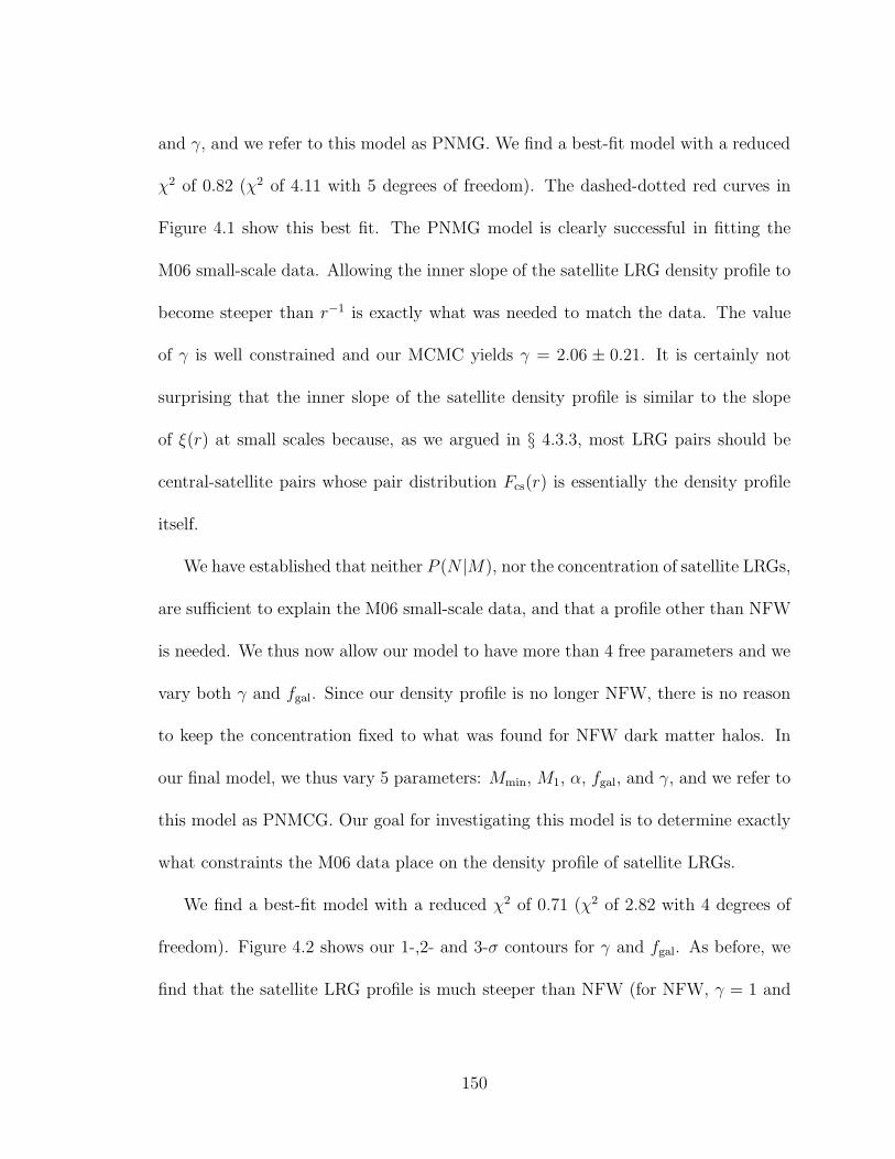
and γ, and we refer to this model as PNMG. We find a best-fit model with a reduced

χ2 of 0.82 (χ2 of 4.11 with 5 degrees of freedom). The dashed-dotted red curves in

Figure 4.1 show this best fit. The PNMG model is clearly successful in fitting the

M06 small-scale data. Allowing the inner slope of the satellite LRG density profile to

become steeper than r−1 is exactly what was needed to match the data. The value

of γ is well constrained and our MCMC yields γ = 2.06 ± 0.21. It is certainly not

surprising that the inner slope of the satellite density profile is similar to the slope

of ξ(r) at small scales because, as we argued in § 4.3.3, most LRG pairs should be

central-satellite pairs whose pair distribution Fcs(r) is essentially the density profile

itself.

We have established that neither P (N |M), nor the concentration of satellite LRGs,

are sufficient to explain the M06 small-scale data, and that a profile other than NFW

is needed. We thus now allow our model to have more than 4 free parameters and we

vary both γ and fgal. Since our density profile is no longer NFW, there is no reason

to keep the concentration fixed to what was found for NFW dark matter halos. In

our final model, we thus vary 5 parameters: Mmin, M1, α, fgal, and γ, and we refer to

this model as PNMCG. Our goal for investigating this model is to determine exactly

what constraints the M06 data place on the density profile of satellite LRGs.

We find a best-fit model with a reduced χ2 of 0.71 (χ2 of 2.82 with 4 degrees of

freedom). Figure 4.2 shows our 1-,2- and 3-σ contours for γ and fgal. As before, we

find that the satellite LRG profile is much steeper than NFW (for NFW, γ = 1 and

150

0.0 0.5 1.0 1.5

1.0

1.5

2.0

γ

fgal0.0 0.5 1.0 1.5

1.0

1.5

2.0

γ

fgal

NFW

SIS

Figure 4.2: Allowed density profiles for LRG satellite galaxies within their dark matter halos.Shaded regions show the 1-σ (red), 2-σ (blue) and 3-σ (green) allowed regions for γ and fgal for thePNMCG model. Filled circles mark the locations of the NFW profile (γ = 1, fgal = 1) and theSingular Isothermal Sphere (SIS) profile (γ = 2, fgal → 0).

fgal = 1), with γ = −2.17± 0.12. As we argued in § 4.3.1, most of the LRG satellites

reside in halos of mass close to M1. At our best-fit value for M1 (1014.62h−1M⊙), the

dark matter concentration fitting formula from § 4.3.1 gives a halo concentration of

c = 4.25. Applying our 1-σ range for fgal implies that cgal ∼ 0.1− 4.1. Concentration

values of unity or less mean that the scale radius rs is larger than the virial radius,

which essentially means that the density profile retains its inner slope most of the

way out. In other words, our fit shows that the density profile for LRG satellites is

consistent with a simple isothermal profile.

151

4.5 Discussion

Our results show that the distribution of satellite LRGs within dark matter halos

requires a steeper inner density profile than NFW, which suggests that these galaxies

are poor tracers of the dark matter distribution at these scales. The density profile

of dark matter halos in the ΛCDM model has been measured extensively using high

resolution N-body simulations, and recent inner profile measurements seem to confirm

the NFW ∼ r−1 predictions (Navarro et al., 2010) – with some slight deviations found

in separate work (Diemand et al., 2004; Fukushige et al., 2004; Reed et al., 2005; Del

Popolo & Kroupa, 2009). However, NFW does not consider baryons, which can af-

fect the dark matter density profile at small scales. The interaction between baryons

and dark matter is addressed by the adiabatic contraction model that describes the

gravitational effect of baryons on dark matter as the gas condenses and sinks to the

center of the dark matter potential well. The gravitational influence of the baryons

draws the dark matter in, and this can steepen the density profile (Gnedin et al.,

2004; Romano-Dıaz et al., 2008; Weinberg et al., 2008; Sommer-Larsen & Limousin,

2009). Although it has been shown that the inner profile can significantly steepen

(Gustafsson et al., 2006), the majority of results show only a moderate steepening.

This has also been observationally confirmed using galaxy-galaxy lensing by Mandel-

baum et al. (2006) who find that the mass density profile of LRG clusters is consistent

with NFW. LRG satellites therefore have a steeper density profile than dark matter

even with the effects of baryons taken into consideration.

152

It is not necessarily surprising that LRGs are poor tracers of the dark matter

density distribution within halos. LRGs presumably live in subhalos, which can

certainly have a different distribution than their host halos. Nagai & Kravtsov (2005)

found that subhalos actually have a shallower profile than dark matter at larger scales,

but this has not been studied for the massive halos and small scales we consider here.

It is difficult to model this regime because simulations must have, both a very large

volume that contains many cluster-sized halos, and high mass and spatial resolution

to resolve scales of ∼ 10h−1kpc. In fact, on these very small scales, it is likely

that dark matter subhalos have already been disrupted by tidal forces, while the

LRGs, being smaller and denser, have survived. So pure dark matter simulations

may be insufficient to predict these LRG results. However, semi-analytic models

that include galaxies and can have arbitrarily high resolution should be able to make

these predictions (see Kitzbichler & White 2008 for semi-analytic modeling of the

very-small scale clustering of lower luminosity galaxies).

In any case, our results have implications for the modeling of LRG clustering

because a standard NFW profile cannot describe the spatial distribution of LRGs

on scales . 0.03h−1Mpc. It would be interesting to see if lower luminosity galaxies

exhibit the same behavior or if this is simply a feature for LRGs. It would also be

interesting to see if LRGs maintain their steep density profile at high redshift.

153

Chapter V

THE EXTREME SMALL SCALES: DO SATELLITE GALAXIES TRACE DARKMATTER?

Abstract

We investigate the radial distribution of galaxies within their host dark mat-

ter halos as measured in the Sloan Digital Sky Survey by modeling their small-

scale clustering. Specifically, we model the Jiang et al. (2011) measurements of

the galaxy two-point correlation function down to very small projected separations

(10 ≤ r ≤ 400h−1kpc), in a wide range of luminosity threshold samples (absolute

r-band magnitudes of −18 up to −23). We use a halo occupation distribution (HOD)

framework with free parameters that specify both the number and spatial distribu-

tion of galaxies within their host dark matter halos. We assume one galaxy resides

in the halo center and additional galaxies are considered satellites that follow a ra-

dial density profile similar to the dark matter Navarro-Frenk-White (NFW) profile,

except that the concentration and inner slope are allowed to vary. We find that in

low luminosity samples (Mr < −19.5 and lower), satellite galaxies have radial profiles

that are consistent with NFW. Mr < −20 and brighter satellite galaxies have radial

profiles with significantly steeper inner slopes than NFW (we find inner logarithmic

slopes ranging from −1.6 to −2.1, as opposed to −1 for NFW). We define a useful

metric of concentration, M1/10, which is the fraction of satellite galaxies (or mass)

154

that are enclosed within one tenth of the virial radius of a halo. We find that M1/10

for low luminosity satellite galaxies agrees with NFW, whereas for luminous galaxies

it is 2.5 − 4 times higher, demonstrating that these galaxies are substantially more

centrally concentrated within their dark matter halos than the dark matter itself.

Our results therefore suggest that the processes that govern the spatial distribution

of galaxies, once they have merged into larger halos, must be luminosity dependent,

such that luminous galaxies become poor tracers of the underlying dark matter.

5.1 Introduction

Determining the relationship between the spatial distributions of galaxies and

dark matter remains one of the central problems of theoretical and observational

cosmology. We saw in Chapter IV that the radial distribution of galaxies within their

host dark matter halos dictates the correlation function on scales smaller than the

virial radii of the largest dark matter halos (. 1h−1Mpc). Therefore, the measured

galaxy correlation function itself is a powerful tool for shedding light on how galaxies

trace the underlying dark matter within halos.

The halo occupation distribution (HOD) framework has been established as a

robust method for modeling galaxy clustering by simply characterizing the biased

relationship between galaxies and mass (see, e.g., Peacock & Smith 2000; Scoccimarro

et al. 2001; Berlind & Weinberg 2002; Cooray & Sheth 2002; Zheng et al. 2005).

The HOD describes this relation by specifying the probability distribution P (N |M)

155

that a halo of mass M contains N galaxies, along with a prescription for the spatial

distribution of galaxies within halos. For this latter component, it is typically assumed

that a single ’central’ galaxy lives at the center of each halo, with additional ’satellite’

galaxies tracing the dominant dark matter component. This assumption has been

used successfully to model galaxy clustering on scales larger than r ∼ 100h−1kpc

(e.g., Zehavi et al., 2004, 2005b, 2011; Zheng et al., 2007, 2009). However, Watson

et al. (2010) showed that this assumption does not work to explain the smaller-scale

clustering of luminous red galaxies (LRGs) in the Sloan Digital Sky Survey (SDSS;

York et al. 2000). In order to achieve a good fit to the clustering of LRGs on scales

smaller than ∼ 100h−1kpc (measured by Masjedi et al., 2006), they found that the

radial profile of satellite LRGs must have a much steeper inner slope compared to

the Navarro-Frenk-White (NFW; Navarro et al. 1997) dark matter profile. Watson

et al. (2010) concluded that the distribution of satellite LRGs within halos is better

described by an isothermal distribution (see Chapter IV for details).

Recently, Jiang et al. (2011) measured the projected two-point correlation function

wp(rp) for several luminosity samples from the SDSS, extending the measurements

done by Zehavi et al. (2011) on intermediate scales (∼ 0.1 − 40h−1Mpc) down to

extremely small galaxy-galaxy separations (0.01−7h−1Mpc). Our motivation for this

paper is to model the innermost data points (0.01 − 0.4h−1Mpc) in the same vein as

Watson et al. (2010, hereafter W10) to see if there is a luminosity dependence of the

156

radial profile of satellite galaxies 1.

The paper is laid out as follows. In §5.2, we review the Jiang et al. (2011, hereafter

J11) measurements. In §5.3, we discuss our modeling method in the following manner:

in §5.3.1 we provide an overview of the general technique used to model the small-

scale correlation function; in §5.3.2 we revisit the W10 four-parameter PNM model

that allows the the probability distribution P (N |M) to vary, and the five-parameter

PNMCG model that also allows the radial distribution of galaxies within halos to vary.

We present our results in §5.4. Finally, we summarize and discuss the implications

of our results in §5.5. Throughout the paper, we assume a ΛCDM cosmology with

Ωm = 0.25,ΩΛ = 0.75,Ωb = 0.04, h0 = 0.7, σ8 = 0.8, ns = 1.0.

5.2 Data

J11 measured the projected two-point correlation function down to very small

scales (0.01 < r < 7h−1Mpc) for a large range of volume-limited galaxy luminosity

threshold samples. Galaxy number densities and median redshifts for each sample can

be found in Table V.1. These samples are constructed from the NYU VAGC (Blanton

et al., 2005) V7.2 data (Abazajian et al., 2009) which contains 8.6× 105 SDSS Main

Sample galaxies (Strauss et al., 2002). Spectra for each luminosity threshold sample

are cross-correlated with the full imaging sample to compute wp(rp) (details of the

method can be seen below). The full imaging sample consists of ∼ 108 galaxies drawn

1Chapter IV is based on W10, thus any reference to W10 in this chapter can be found in Chap-ter IV

157

from the SDSS imaging catalog.

Measuring wp(rp) on very small scales is a non-trivial task. The SDSS spectro-

scopic sample suffers from incompleteness due to the physical size of the fiber-optic

cables, which impede the ability to take spectra of two galaxies closer than 55′′ on

the sky. These “fiber collisions” thus result in a minimum pair separation of 55′′.

This effect is partially mitigated by the tiling method (Blanton et al., 2003), which

overlaps spectroscopic plates in order to yield full sky coverage. In plate overlap re-

gions, galaxy pairs closer than 55′′ can be recovered. However, this still leaves ∼ 9%

of galaxies without measured redshifts (J11) and this can strongly affect clustering

measurements on very small scales. Following the approach described in Masjedi

et al. (2006, 2008), J11 used a cross-correlation technique between the imaging and

spectroscopic samples to correct for fiber collisions and obtain unbiased wp(rp) mea-

surements down to the 10h−1kpc scale. Details of the method can be found in §5.3

of J11.

A second potential problem that affects very small scales is that galaxies may be

overlapping and the light within this region needs to be properly distributed between

the two galaxies. This is known as “deblending”. M06 found a systematic error in the

SDSS pipeline wherein too much light was allocated to the dimmer of the two galax-

ies. As a result, a galaxy that may have been too dim to make the LRG brightness cut

could now be included in the sample. This increased the number of small-scale pairs

and boosted the correlation function on very small scales. M06 quantified this effect

158

and corrected their measurements accordingly. Since the physical sizes of galaxies

decrease rapidly with decreasing luminosity, this photometric deblending error di-

minishes in lower luminosity samples. For this reason, J11 ignored this effect in the

luminosity samples they considered (Mr < −18 through −21). Nevertheless, we esti-

mate the maximum effect of deblending by applying the M06 LRG correction to the

Mr < −21 sample and repeating our analysis. We find that our results do not change

qualitatively.

We restrict ourselves to modeling the J11 data points from ∼ 10 − 400h−1kpc.

These can be seen in Figure 5.1, which shows wp(rp) scaled by an r−1p power law,

with each panel corresponding to a distinct luminosity threshold. The bottom right

panel of Figure 5.1 shows the LRG data points measured by M06 and modeled by

W10. Along with these 9 data points used in our modeling, we also incorporate the

measured number density for each luminosity sample (see Table V.1), providing a

tenth data point. We use the full covariance matrices from the 9 J11 wp(rp) data

points for each sample, which were estimated using jackknife resampling of 50 regions

on the sky. The same jackknife samples were used to estimate the error on each

calculated number density.

159

5.3 Review of the Method

5.3.1 The HOD and the Galaxy 2PCF

Here we briefly review the method used in W10, which is based on the halo

occupation distribution (HOD) formalism. The HOD fully characterizes the number,

velocity and spatial distribution of galaxies within dark matter halos. The probability

distribution that a virialized dark matter halo of mass M will host N galaxies is

designated as P (N |M). 〈N〉M is the first moment of P (N |M), and is the mean

number of galaxies as a function of halo mass. Motivated by theory (e.g., Berlind

et al., 2003; Kravtsov et al., 2004a; Zheng et al., 2005), we consider central galaxies

that live at the center of their host halo and satellite galaxies that orbit within the

host potential as separate terms. We thus write the first moment of the HOD as

〈N〉M = 1 + 〈Nsat〉M . Furthermore, we assume that there is some minimum halo

mass, Mmin, below which a halo will contain no galaxies and above which there will

always be at least one central galaxy. For the satellite component, we adopt the

parametric form, 〈Nsat〉M = exp[−M0/(Mhalo − Mmin)] × (Mhalo/M1)α, where the

satellite galaxies obey a power-law function of slope α with an exponential cut-off at

the low mass end at M0. M1 is the characteristic mass scale where a halo will contain,

on average, one central and one satellite galaxy.

To calculate the mean number of satellite galaxy pairs 〈Nsat(Nsat −1)〉,the second

moment of the satellite P (N |M), we assume that the number of satellite galaxies

in a halo of mass M follows a Poisson distribution of mean 〈Nsat〉M . This sort of

160

HOD parameterization is widely used to model galaxy clustering data (Zehavi et al.,

2005a,b, 2011; Tinker et al., 2005; Conroy et al., 2006; Zheng et al., 2007, 2009;

Watson et al., 2011b).

Our fiducial model for characterizing the spatial distribution of galaxies within

their host halos places one galaxy at the center and assuming that the satellites trace

the underlying dark matter density distribution. The dark matter density profiles are

described by the NFW relation ρ(r) ∝ (c rRvir

)−1(1 + c rRvir

)−2 (Navarro et al., 1997),

where c is the concentration parameter, c ≡ Rvir/rs, and rs is the characteristic scale

radius. We use the virial definition of a halo to calculate the virial radius of host

halos, such that Rvir = ((3M)/(4π∆virρ))1/3, where ∆vir is the mean halo overdensity

(∆vir = 200), and ρ is the mean density of the universe. The concentration - mass

relation is given by Zheng et al. (2007) for the modification of Bullock et al. (2001):

c = c0(1+z)

× (Mhalo

M∗

)−β, where c0 = 11, M∗ is the non-linear collapse mass at the

median redshift of the sample for our choice of cosmology (M∗ is redshift dependent

and is thus uniquely defined for each luminosity sample and is given in Table V.1)

and β = 0.13.

The mean number density of galaxies can be calculated for a given HOD by

weighting the abundance of halos by 〈N〉M and integrating over all halo mass (see

Eq.[2] of W10). We adopt the Warren et al. (2006) halo mass function, dn/dM , in

all of our calculations, but our results are not sensitive to the specific choice of mass

function.

161

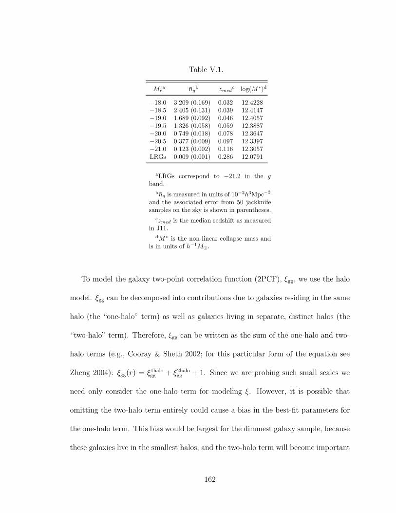
Table V.1.

Mra ng

b zmedc log(M∗)d

−18.0 3.209 (0.169) 0.032 12.4228−18.5 2.405 (0.131) 0.039 12.4147−19.0 1.689 (0.092) 0.046 12.4057−19.5 1.326 (0.058) 0.059 12.3887−20.0 0.749 (0.018) 0.078 12.3647−20.5 0.377 (0.009) 0.097 12.3397−21.0 0.123 (0.002) 0.116 12.3057LRGs 0.009 (0.001) 0.286 12.0791

aLRGs correspond to −21.2 in the gband.

bng is measured in units of 10−2h3Mpc−3

and the associated error from 50 jackknifesamples on the sky is shown in parentheses.

czmed is the median redshift as measuredin J11.

dM∗ is the non-linear collapse mass andis in units of h−1M⊙.

To model the galaxy two-point correlation function (2PCF), ξgg, we use the halo

model. ξgg can be decomposed into contributions due to galaxies residing in the same

halo (the “one-halo” term) as well as galaxies living in separate, distinct halos (the

“two-halo” term). Therefore, ξgg can be written as the sum of the one-halo and two-

halo terms (e.g., Cooray & Sheth 2002; for this particular form of the equation see

Zheng 2004): ξgg(r) = ξ1halogg + ξ2halo

gg + 1. Since we are probing such small scales we

need only consider the one-halo term for modeling ξ. However, it is possible that

omitting the two-halo term entirely could cause a bias in the best-fit parameters for

the one-halo term. This bias would be largest for the dimmest galaxy sample, because

these galaxies live in the smallest halos, and the two-halo term will become important

162

at small scales. However, even for these galaxies the effect is limited. For instance,

while it is true that isolated −18 galaxies will reside in halos with radii much smaller

than 0.4h−1Mpc, the relevant halo size is set by M1. Furthermore, this is a threshold

sample, so although the −18 sample will be dominated by galaxies of that brightness,

there will still be much brighter galaxies that live in larger halos that influence M1.

As seen in the upper-left panel of Fig. 5.3, 〈M1〉 for the −18 sample is 1012.77. This

corresponds to a virial radius of order 0.4h−1Mpc. To carefully test the influence of

the two-halo term, we have have measured where the 1- and 2-halo terms cross for

the −18 sample. This occurs at roughly 1h−1Mpc, so the influence of the 2-halo term

at 0.4h−1Mpc has a small effect on wp(rp). We find that the amplitude of the 2-halo

term is ∼ 7% of the one-halo term at 0.4h−1Mpc for the −18 sample. Nevertheless,

we do approximately account for the effect of the 2-halo term on our modeling, and

we discuss these assumptions in detail below.

The one-halo term depends on the second moment of P (N |M), as well as the pair

separation distributions of central-satellite and satellite-satellite pairs (see Eq.[4] of

W10 for the particular form). The pair separation distribution for central-satellite

pairs is essentially the same as the density profile of satellite galaxies. The satellite-

satellite pair distribution is the convolution of the density profile with itself and, as

in W10, we use the Sheth et al. (2001) calculation for the convolution of a truncated

NFW profile with itself. Therefore, we can start to see the link between the shape of

ξ(r) and the shape of the satellite profile on small scales. This is discussed in detail

163

in §5.4.

For each luminosity threshold, J11 measured the projected correlation function,

so we convert our theoretical real-space correlation function ξ(r) to wp(rp) (Eq.[5] of

W10). At each luminosity threshold, we integrate up to the πmax value given in Zehavi

et al. (2011), which ranges from 40−60h−1Mpc. The method of J11 results in a πmax

that is effectively larger than our choice. However, the difference is insignificant at

the small scales we model. Integrating out to large scales means that the two-halo

term cannot be entirely ignored. Since calculating the two-halo term correctly is fairly

complex and its contribution to wp(rp) is minimal at the scales of the data points that

we model, we use a simple approximation instead. We use a two-halo term whose

shape is the same as Zehavi et al. (2011), but whose amplitude can change with

HOD parameters. Thus, for a given set of HOD parameters, we first calculate the

large-scale bias of galaxies, bg,

bg = n−1g

∫

∞

Mmin

dMdn

dMbh(M)〈N〉M , (5.1)

where bh(M) is the large-scale bias of halos from Tinker et al. (2008). The two-halo

term has a simple relation to the matter-matter correlation function on large scales:

ξ2halogg = b2gξmm. Thus, the relative two-halo terms of two different galaxy samples

really only depends on the ratio of the bias of each sample. We consider the best-

fit two-halo term from Zehavi et al. (2011) for each luminosity and append a newly

164

defined two-halo term to our model one-halo term,

ξ2halogg =

( bgb ′g

)2

ξ2halo ′

gg , (5.2)

where primes designate the Zehavi et al. (2011) values. In effect, we allow the am-

plitude of the 2-halo term to vary with HOD parameters, but we keep its shape

fixed. The error introduced by this approximation is completely negligible as we have

checked that even a shift as large as 20% in the amplitude of the two-halo term has

no appreciable effect on wp(rp) at the maximum pair separation that we consider

(0.4h−1Mpc) for any of the luminosity threshold samples. This test also emphasizes

our insensitivity to the difference between our choice of integrating out to the πmax

given by Zehavi et al. (2011) and the technique used by J11.

5.3.2 The PNM and PNMCG Models

W10 considered 4 distinct models for modeling the small-scale wp(rp) of LRGs.

In this paper we need only consider two of the models, defined as:

• PNM - in this model the only free parameters are those associated with the

P (N |M) distribution as described in §5.3.1 - Mmin,M0,M1, and α. While these

parameters are free to take on any value, the spatial distribution of satellite

galaxies within halos is fixed to an NFW dark matter density profile. Since

there are 10 data points (9 from the J11 wp(rp) measurements along with the

165

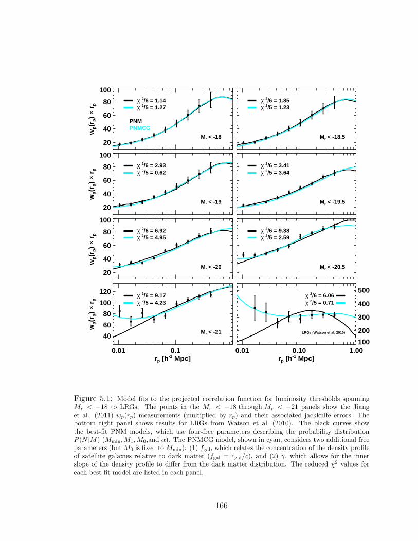
20

40

60

80

100w

p(r

p)

× r p

χ 2/6 = 1.14χ 2/5 = 1.27

PNMCGPNM

Mr < -18

χ 2/6 = 1.85χ 2/5 = 1.23

Mr < -18.5

20

40

60

80

100

wp(r

p)

× r p

χ 2/6 = 2.93χ 2/5 = 0.62

Mr < -19

χ 2/6 = 3.41χ 2/5 = 3.64

Mr < -19.5

20

40

60

80

100

wp(r

p)

× r p

χ 2/6 = 6.92χ 2/5 = 4.95

Mr < -20

χ 2/6 = 9.38χ 2/5 = 2.59

Mr < -20.5

0.01 0.1 rp [h

-1 Mpc]

40

60

80

100

120

wp(r

p)

× r p

χ 2/6 = 9.17χ 2/5 = 4.23

Mr < -21

0.01 0.10 1.00rp [h

-1 Mpc]

100

200

300

400

500χ 2/6 = 6.06χ 2/5 = 0.71

LRGs (Watson et al. 2010)

Figure 5.1: Model fits to the projected correlation function for luminosity thresholds spanningMr < −18 to LRGs. The points in the Mr < −18 through Mr < −21 panels show the Jianget al. (2011) wp(rp) measurements (multiplied by rp) and their associated jackknife errors. Thebottom right panel shows results for LRGs from Watson et al. (2010). The black curves showthe best-fit PNM models, which use four-free parameters describing the probability distributionP (N |M) (Mmin,M1,M0,and α). The PNMCG model, shown in cyan, considers two additional freeparameters (but M0 is fixed to Mmin): (1) fgal, which relates the concentration of the density profileof satellite galaxies relative to dark matter (fgal = cgal/c), and (2) γ, which allows for the innerslope of the density profile to differ from the dark matter distribution. The reduced χ2 values foreach best-fit model are listed in each panel.

166

measured number density for each luminosity sample) and 4 free parameters,

the PNM model has 6 degrees of freedom.

• PNMCG - this model allows for the same free parameters as the PNM model,

with the exception of M0. M0 was unconstrained in our initial MCMC runs (this

was also the case in W10), thus we fixed M0 to Mmin throughout our analysis.

The PNMCG model also considers a parametrized density profile for satellite

galaxies. As in W10, we allow both the concentration and the inner slope of the

density profile to be free. The satellite galaxy concentration can differ from the

dark matter concentration (defined in §5.3.1) through the free parameter fgal,

cgal = fgal × c. (5.3)

The inner slope of the density profile is no longer fixed to -1, as is the case for

an NFW profile, but rather is specified by the free parameter γ. As in W10, we

adopt the following density profile for satellite galaxies

ρ(r) =ρs

(cgalr

Rvir

)γ(1 + cgalr

Rvir

)3−γ. (5.4)

For an NFW profile γ = 1, however, the PNMCG model allows γ to take on

any value from 0 − 4. This model considers the same number of data points as

the PNM model, but now there are 5 free parameters (Mmin,M1, α, fgal and γ)

resulting in 5 degrees of freedom.

167

As detailed in §3.4 of W10, we use a Markov Chain Monte Carlo (MCMC) method

to probe the parameter space for a given set of parameters (see Dunkley et al. 2005

for details on MCMC techniques). When a chain has converged, we can find the most

likely value for each parameter by calculating the mean of its distribution. Errors

for each parameter are given by the extrema of the middle 68.3% of the distribution.

Best-fit parameters are found by the combination of parameter values for which χ2 is

a minimum.

5.4 Results

J11 measured wp(rp) to very small scales over a large range in luminosity thresh-

olds. Their measurements nicely overlap those of Zehavi et al. (2011) on intermediate

scales (∼ 0.2−7h−1Mpc, see Fig. 14 in J11), and extend down to very small scales with

the innermost data point for each sample at ∼ 10h−1kpc. As discussed in §5.3.2, for

each luminosity threshold sample, we model wp(rp) with, (1) the PNM model, which

only varies parameters that determine the number of galaxies in a given halo, but

forces the satellite galaxies to have an NFW spatial distribution within their halo,

and (2) the PNMCG model, which also allows the spatial distribution of satellite

galaxies to vary within halos.

Figure 1 shows our modeling results for each luminosity sample. wp(rp) has been

scaled by an r−1p power law to more clearly highlight any discrepancies between the

PNM and PNMCG models. Each panel shows the SDSS data points as well as the

168

best-fit model for the PNM (black curve) and PNMCG (cyan curve) cases. It is clear

from the figure that as we go to higher luminosities, the PNMCG model provides a

significantly better fit to the data. We find that the P (N |M) parameter distributions

are nearly the same for the two models, differing by, at most, ∼ 3σ. Therefore, the

improved fits for the PNMCG model principally arise from the freedom to vary the

density profile of satellite galaxies. Varying the density profile is thus necessary to

find a better fit to the data as we go to higher luminosities.

We note that the reduced χ2 values (listed in each panel) are in many cases quite

high, even in the PNMCG case. This could mean that the PNMCG model contains

incorrect assumptions or does not have enough freedom. On the other hand, it could

mean that the J11 jackknife errors are underestimated. To check the impact of the

error estimates on our modeling, we re-estimated errors for the Mr < −20 sample

using mock galaxy catalogs from the LasDamas project (McBride et al. in prep.).

We used 160 catalogs 1 and measured the dispersion of wp(rp) between the catalogs,

using the same binning method as J11. We then applied the fractional error (with

respect to the mean of all mock measurements) to the data (non-mock) measurement

to estimate the absolute errors and full covariance. Finally, using our new mock

based error estimates, we re-ran the MCMC chains for the PNMCG model. We then

compared the best-fit parameter values for the two fits and found that the parameters

did not change significantly. By this, we mean the difference in χ2 between the two

1North-only SDSS footprint from the LasDamas ”gamma” data release.

169

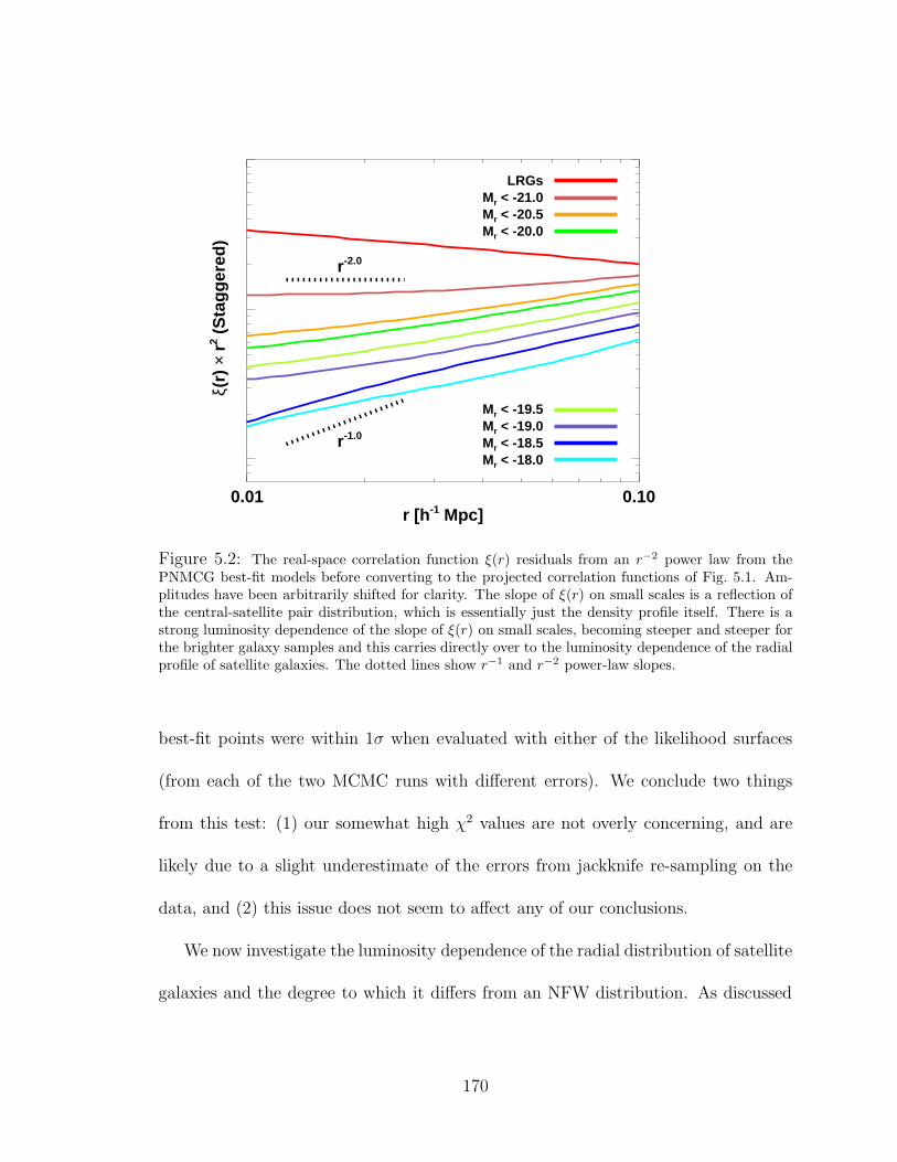
0.01 0.10r [h-1 Mpc]

ξ(r)

× r

2 (S

tag

ger

ed)

r-2.0

r-1.0

LRGsMr < -21.0Mr < -20.5Mr < -20.0

Mr < -18.0Mr < -18.5Mr < -19.0Mr < -19.5

Figure 5.2: The real-space correlation function ξ(r) residuals from an r−2 power law from thePNMCG best-fit models before converting to the projected correlation functions of Fig. 5.1. Am-plitudes have been arbitrarily shifted for clarity. The slope of ξ(r) on small scales is a reflection ofthe central-satellite pair distribution, which is essentially just the density profile itself. There is astrong luminosity dependence of the slope of ξ(r) on small scales, becoming steeper and steeper forthe brighter galaxy samples and this carries directly over to the luminosity dependence of the radialprofile of satellite galaxies. The dotted lines show r−1 and r−2 power-law slopes.

best-fit points were within 1σ when evaluated with either of the likelihood surfaces

(from each of the two MCMC runs with different errors). We conclude two things

from this test: (1) our somewhat high χ2 values are not overly concerning, and are

likely due to a slight underestimate of the errors from jackknife re-sampling on the

data, and (2) this issue does not seem to affect any of our conclusions.

We now investigate the luminosity dependence of the radial distribution of satellite

galaxies and the degree to which it differs from an NFW distribution. As discussed

170

in §5.3.1, when constructing the real-space correlation function in the halo model,

the one-halo term considers contributions from central-satellite and satellite-satellite

pairs. The central-satellite contribution, which is essentially just the density profile

itself (see Eq. 4 of W10), is steeper than the satellite-satellite pair contribution and

thus dominates the correlation function on the very small scales that we are consid-

ering (e.g., Figure 4. of Zheng et al., 2009). Therefore, the luminosity dependence of

the slope of ξ(r) on small scales can give a direct indication of the luminosity depen-

dence of the radial profile of satellite galaxies (though the slope of ξ(r) will be less

steep than the slope of the radial density profile due to the dampening effect of the

satellite-satellite term). Figure 5.2 shows the residuals from an r−2 power law from

the PNMCG best-fit models before converting to the projected correlation functions

shown in Figure 5.1. The amplitudes of the curves have been arbitrarily staggered

simply to make the plot more clear. The dotted lines highlight the cases of r−1 and

r−2 power laws. The slope of ξ(r) is clearly a strong function of luminosity, being

close to -1 for low luminosity galaxies and going more and more towards -2 for the

Mr < −21 sample and even steeper for LRGs. The W10 result for the steepness of

the slope of ξ(r) for LRGs on small scales was also found by Almeida et al. (2008).

Using the Bower et al. (2006) semi-analytic model applied to the Millenium simula-

tion (Springel et al., 2005), they found that the LRG real-space correlation function

follows an ∼ r−2.07 power law shape down to the ∼ 10h−1kpc scale.

We next wish to directly investigate the radial profiles of satellite galaxies that

171

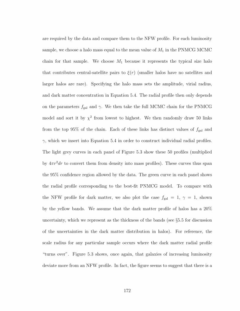
are required by the data and compare them to the NFW profile. For each luminosity

sample, we choose a halo mass equal to the mean value of M1 in the PNMCG MCMC

chain for that sample. We choose M1 because it represents the typical size halo

that contributes central-satellite pairs to ξ(r) (smaller halos have no satellites and

larger halos are rare). Specifying the halo mass sets the amplitude, virial radius,

and dark matter concentration in Equation 5.4. The radial profile then only depends

on the parameters fgal and γ. We then take the full MCMC chain for the PNMCG

model and sort it by χ2 from lowest to highest. We then randomly draw 50 links

from the top 95% of the chain. Each of these links has distinct values of fgal and

γ, which we insert into Equation 5.4 in order to construct individual radial profiles.

The light grey curves in each panel of Figure 5.3 show these 50 profiles (multiplied

by 4πr2dr to convert them from density into mass profiles). These curves thus span

the 95% confidence region allowed by the data. The green curve in each panel shows

the radial profile corresponding to the best-fit PNMCG model. To compare with

the NFW profile for dark matter, we also plot the case fgal = 1, γ = 1, shown

by the yellow bands. We assume that the dark matter profile of halos has a 20%

uncertainty, which we represent as the thickness of the bands (see §5.5 for discussion

of the uncertainties in the dark matter distribution in halos). For reference, the

scale radius for any particular sample occurs where the dark matter radial profile

“turns over”. Figure 5.3 shows, once again, that galaxies of increasing luminosity

deviate more from an NFW profile. In fact, the figure seems to suggest that there is a

172

transition point, somewhere between an absolute r-band magnitude of -19.5 and -20,

where the radial profile of satellite galaxies goes from being consistent with NFW to

completely inconsistent. For the highest luminosity samples, the profiles approach a

power-law shape.

Figure 5.4 shows the luminosity dependence of the inner slope and concentration of

satellite galaxies as found by the PNMCG model. The dark blue and light blue bands

in each panel represent the middle 95% and 68.3% of the MCMC chains after first

sorting in γ (top panel) and sorting in fgal (bottom panel). The filled red squares show

the mean of the respective parameters in the MCMC chain for each luminosity sample

and filled green squares show the best-fit values. The solid black line highlights the

NFW dark matter inner slope of the density profile which corresponds to γ = fgal = 1

and the dotted lines represent the possible 20% ambiguity of an assumed NFW inner

slope and concentration. The Mr < −18,−18.5,−19 and − 19.5 samples have large

spreads in γ and fgal values, as there are many parameter combinations that can

yield a similar goodness-of-fit to the data. For Mr < −20 and brighter galaxies, both

γ and fgal have tighter distributions and deviate from NFW. Figure 5.4 shows that

there is a strong luminosity dependence of the satellite galaxy profile, i.e. γ is an

increasing function of luminosity, and fgal is a decreasing one. However, notice the

unique coupling of fgal and γ for the −20.5 case, where fgal seems to deviate from the

aforementioned trend. γ for −20.5 satellite galaxies also strays from the trend, but

it is still significantly larger than NFW, and still lies within 1σ of the Mr < −20 and

173

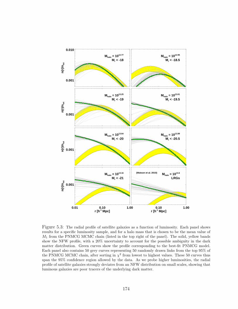
0.001

0.010

n(r

)/n

tot

Mhalo = 1012.77

Mr < -18

Mhalo = 1012.95

Mr < -18.5

0.001

n(r

)/n

tot

Mhalo = 1013.25

Mr < -19

Mhalo = 1013.61

Mr < -19.5

0.001n(r

)/n

tot

Mhalo = 1013.64

Mr < -20

Mhalo = 1013.89

Mr < -20.5

0.01 0.10 1.00r [h-1 Mpc]

0.001

n(r

)/n

tot

Mhalo = 1014.16

Mr < -21

0.10 1.00r [h-1 Mpc]

Mhalo = 1014.6

LRGs

(Watson et al. 2010)

Figure 5.3: The radial profile of satellite galaxies as a function of luminosity. Each panel showsresults for a specific luminosity sample, and for a halo mass that is chosen to be the mean value ofM1 from the PNMCG MCMC chain (listed in the top right of the panel). The solid, yellow bandsshow the NFW profile, with a 20% uncertainty to account for the possible ambiguity in the darkmatter distribution. Green curves show the profile corresponding to the best-fit PNMCG model.Each panel also contains 50 grey curves representing 50 randomly drawn links from the top 95% ofthe PNMCG MCMC chain, after sorting in χ2 from lowest to highest values. These 50 curves thusspan the 95% confidence region allowed by the data. As we probe higher luminosities, the radialprofile of satellite galaxies strongly deviates from an NFW distribution on small scales, showing thatluminous galaxies are poor tracers of the underlying dark matter.

174

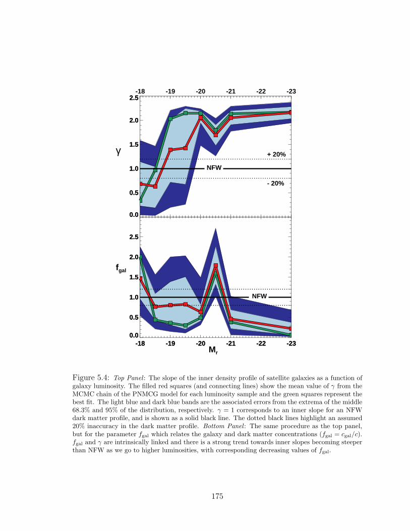
0.0

0.5

1.0

1.5

2.0

2.5

γNFW

+ 20%

- 20%

-18 -19 -20 -21 -22 -23

0.0

0.5

1.0

1.5

2.0

2.5

-18 -19 -20 -21 -22 -230.0

0.5

1.0

1.5

2.0

2.5

fgal

Mr

NFW

-18 -19 -20 -21 -22 -230.0

0.5

1.0

1.5

2.0

2.5

Figure 5.4: Top Panel : The slope of the inner density profile of satellite galaxies as a function ofgalaxy luminosity. The filled red squares (and connecting lines) show the mean value of γ from theMCMC chain of the PNMCG model for each luminosity sample and the green squares represent thebest fit. The light blue and dark blue bands are the associated errors from the extrema of the middle68.3% and 95% of the distribution, respectively. γ = 1 corresponds to an inner slope for an NFWdark matter profile, and is shown as a solid black line. The dotted black lines highlight an assumed20% inaccuracy in the dark matter profile. Bottom Panel : The same procedure as the top panel,but for the parameter fgal which relates the galaxy and dark matter concentrations (fgal = cgal/c).fgal and γ are intrinsically linked and there is a strong trend towards inner slopes becoming steeperthan NFW as we go to higher luminosities, with corresponding decreasing values of fgal.

175

Mr < −21 values (fgal is within 2σ). However, the reason for this outlier is unclear,

though it may be due to the fact that wp(rp) has a strong feature at roughly the scale

radius of the typical host halo (see the Mr < −20.5 panel of Fig. 5.1). This may cause

a unique interplay between fgal and γ, resulting in a mild departure from the trends.

For Mr < −20 and brighter galaxies, the mean value of γ ranges between 1.6 - 2.1,

significantly steeper than NFW. This range of γ values persists all the way down to

Mr < −19 when considering the best-fit values. As mentioned in §5.2, M06 found a

systematic error in the manner that light in the overlapping region of LRG pairs was

being allocated in the SDSS pipeline. This caused a slight boost in the small-scale

correlation function and was corrected for by M06. This effect is expected to rapidly

diminish for lower luminosity samples, because the intrinsic sizes of galaxies will be

smaller. However, we apply the same LRG correction to the J11 Mr < −21 sample

to model the maximum effect that this could have. While we expect 〈γ〉 to decrease

as a result of the innermost data points being scaled to lower wp(rp) values, we still

find that 〈γ〉 ∼ 1.6. Thus, even after assuming a drastic over-correction, γ is still

strongly discrepant from NFW.

Figure 5.4 showed the luminosity trends for γ and fgal by sorting the MCMC

chains separately for each parameter. However, γ and fgal are intrinsically coupled

to one another so it is important to investigate the joint γ − fgal parameter space.

Figure 5.5 Shows the γ − fgal parameter space at each luminosity, with the dark

blue and light blue regions defined as the top 95% and 68.3% of the MCMC chain,

176

0.0

0.5

1.0

1.5

2.0

2.5

γ

NFWSIS Mr < -18

Mr < -18.5

0.0

0.5

1.0

1.5

2.0

2.5

γ

Mr < -19

Mr < -19.5

0.0

0.5

1.0

1.5

2.0

2.5

γ

Mr < -20

Mr < -20.5

0.0 0.5 1.0 1.5 2.0 0.0

0.5

1.0

1.5

2.0

2.5

γ

fgal

Mr < -21

0.0 0.5 1.0 1.5 2.0 2.5

fgal

LRGs

Figure 5.5: The γ− fgal parameter space as a function of luminosity, highlighting the relationshipbetween the inner slope and concentration of the density profile of satellite galaxies relative to darkmatter. For each panel, the dark blue and light blue regions are defined as the top 95% and 68.3% ofthe MCMC chain for a given luminosity sample after sorting in χ2. There are two points of referencedesignated as filled circles - the γ = 1, fgal = 1 combination that represents an NFW distribution,and the γ = 2, fgal → 0 combination that represents a singular isothermal sphere distribution (SIS).Red squares show the mean values of γ and fgal from our MCMC runs and green squares show thevalues for the best-fit model. The data for Mr < −20 and brighter galaxies strongly rule out theNFW model and are in good agreement with an SIS distribution for Mr < −21 and LRGs.

177

after sorting in χ2. There are two points of reference designated as filled circles:

the γ = 1, fgal = 1 combination for an NFW distribution and a γ = 2, fgal → 0

combination representing a singular isothermal sphere (SIS) distribution. Red squares

represent the mean values of γ and fgal from our MCMC runs and green squares show

the best-fit combination. As expected, the Mr < −18 through −19.5 exhibit a broad

range in γ−fgal combinations, with the NFW combination lying within the top 68.3%

region (with the exception of the -18.5 sample). The γ−fgal regions clearly drift away

from NFW for Mr < −20 and greater luminosities and are well described by an SIS

distribution for both the −21 and LRG samples. Figure 5.5 shows that the inner slope

and concentration parameters are strongly degenerate with each other, particularly

at low luminosities. This can be caused by having the scale radius (the radius within

the halo where the slope transitions from −γ to -3) too close to the innermost data

point. When this happens, the data cannot accurately constrain the inner slope, and

only constrains γ and fgal through their degenerate contribution to the amplitude of

the density profile. A simple calculation of the scale radius using the virial definition

of a halo (see §5.3.1) gives rs ∼ 10h−1kpc for the Mr < −18 sample (adopting a halo

mass equal to the mean value of M1), which is precisely at the scale of the innermost

data point of wp(rp). This leads to the large spread in γ − fgal combinations. Of

course, as we go to brighter samples, the scale radii increase, and the parameters are

better constrained.

For each luminosity, as the inner profile steepens, fgal decreases (with the slight

178

deviation for the Mr < −20.5 case). The decrease in concentration does not neces-

sarily imply that the concentration of satellites is low in the traditional sense - i.e.,

that there are fewer galaxies at small radii - but rather that the radial profiles simply

evolve toward a more power-law form. For example, as fgal → 0 in the case of LRGs,

this does not mean that the LRG satellites are less concentrated than the underlying

dark matter. As fgal → 0, the scale radius is pushed far outside the virial radius,

resulting in a pure power-law distribution of slope −γ. Since the value of fgal can be

misleading when thinking about the concentration of satellite galaxies, we consider an

alternative definition of “concentration” that is more physically useful: the fraction

of satellite galaxies (or mass) that are enclosed within a tenth of the virial radius Rvir.

We call this quantity M1/10 and compute it by integrating any radial profile out to

one-tenth the virial radius of the host halo and dividing by the total mass out to Rvir

M1/10 =M(r < 0.1Rvir)

M(r < Rvir). (5.5)

Figure 5.6 (top panel) shows M1/10 as a function of luminosity. For each luminosity

sample, we assume a halo mass equal to the mean value of M1 from the MCMC chain,

and we calculateM1/10 for every link in the chain using each link’s values for γ and fgal.

We then find the mean of the distribution of M1/10 values (denoted by the red squares

and connecting lines). Errors for M1/10 are given by the extrema of the middle 68.3%

of the distribution after sorting byM1/10. The black filled circles show M1/10 for a dark

matter NFW profile. The dark matter concentration drops with luminosity because

179

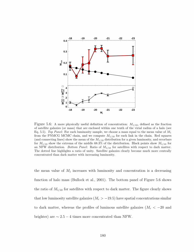
0.1

0.2

0.3

0.4

M1/

10

-18 -19 -20 -21 -22 -23

-18 -19 -20 -21 -22 -23Mr

0

1

2

3

4

⟨M1/

10S

ats ⟩

/ ⟨M

1/10

NF

W

⟩

Figure 5.6: A more physically useful definition of concentration: M1/10, defined as the fractionof satellite galaxies (or mass) that are enclosed within one tenth of the virial radius of a halo (seeEq. 5.5). Top Panel : For each luminosity sample, we choose a mass equal to the mean value of M1

from the PNMCG MCMC chain, and we compute M1/10 for each link in the chain. Red squares(and connecting lines) show the mean of the M1/10 distribution for a given luminosity, and errorbarsfor M1/10 show the extrema of the middle 68.3% of the distribution. Black points show M1/10 foran NFW distribution. Bottom Panel : Ratio of M1/10 for satellites with respect to dark matter.The dotted line highlights a ratio of unity. Satellite galaxies clearly become much more centrallyconcentrated than dark matter with increasing luminosity.

the mean value of M1 increases with luminosity and concentration is a decreasing

function of halo mass (Bullock et al., 2001). The bottom panel of Figure 5.6 shows

the ratio of M1/10 for satellites with respect to dark matter. The figure clearly shows

that low luminosity satellite galaxies (Mr > −19.5) have spatial concentrations similar

to dark matter, whereas the profiles of luminous satellite galaxies (Mr < −20 and

brighter) are ∼ 2.5 − 4 times more concentrated than NFW.

180

5.5 Summary & Discussion

Do satellite galaxies trace the underlying dark matter distribution? Our modeling

of the small-scale wp(rp) over an enormous range in galaxy luminosity thresholds,

from SDSS Main galaxies to LRGs (Mr < −18 through . −23), has revealed a

strong luminosity dependence of the radial distribution of satellite galaxies. We have

found that for the low luminosity samples (lower than Mr < −20), there is a wide

range of satellite galaxy concentrations (equal to fgal times the NFW dark matter

concentration) and inner density profile slopes, −γ, that are consistent with the data.

This lack of constraining power is due to a strong degeneracy between fgal and γ,

which, in turn, is possibly due to the fact that the smallest scale data point in wp(rp)

is roughly around the scale radius for halos hosting galaxies of this size. Nevertheless,

low luminosity satellite galaxies have radial distributions that are generally consistent

with the NFW dark matter distribution. When we move to higher luminosity galaxies

(Mr < −20 and brighter samples) however, satellite profiles change dramatically,

with the most striking feature being that γ jumps to much higher values. Our results

show that for Mr < −20 and brighter galaxies, γ ranges from ∼ 1.6 − 2.1, highly

discrepant from NFW, even after assuming a 20% inaccuracy in the dark matter

profile. Luminous satellite galaxies are thus poor tracers of the underlying dark

matter within halos on the small scales that we probe. Since the effects of fgal and

γ on the radial profile are intertwined, we have calculated a more physically useful

quantity M1/10, which gives the fractional amount of mass enclosed within one-tenth

181

of the virial radius. We find that M1/10 is a strong function of luminosity, being

consistent with NFW for low luminosity galaxies and being ∼ 2.5 − 4 times more

concentrated than NFW for galaxies brighter than Mr < −20.

Several other studies have also investigated the radial distribution of galaxies

within halos. When considering faint satellites around ∼ L∗ galaxies, no consensus

emerges. Chen (2009) found the satellite distribution to be consistent with NFW.

More et al. (2009) found a cored satellite profile best described by a γ = 0, fgal = 0.5

combination, inconsistent with NFW. Carlberg et al. (2009) found that the radial

profiles of dwarf satellites around nearby galaxies are much more concentrated than

NFW, rendering all of these studies in disaccord. Furthermore, the discrepancies

persist when considering a broader range of galaxy systems. Nierenberg et al. (2011)

recently studied the radial profile of satellites around massive, early-type galaxies

at intermediate redshifts. Assuming a power-law profile model, they find that the

satellites have an isothermal distribution of slope -1. Guo et al. (2012) considered

SDSS satellite galaxies around host central galaxies of a wide luminosity range and,

in general, satellite number density profiles were shown to be consistent with NFW.

The NFW dark matter concentration was found to decrease with increasing satellite

galaxy luminosity, independent of the host galaxy luminosity (except for the brightest

centrals). They also detected a slightly steeper profile for fainter satellites. These

varying results imply that uncovering the spatial distribution of satellite galaxies is

a difficult problem. In the end, we have found that there is a strong luminosity

182

dependence of the radial distribution of satellite galaxies, wherein ∼ L∗ and brighter

satellites within group and cluster sized halos have a substantially steeper radial profile

than dark matter on scales smaller than ∼ 100h−1kpc. We emphasize that while the

scales involved in all of these studies are similar to ours, galaxy sample selection is

different in each case, making it difficult to directly compare their results with ours.

Our results have shown that luminous galaxies are poor tracers of NFW. We now

address the possibility that NFW is a poor model for the underlying dark matter

distribution. In the established ΛCDM concordance cosmology, recent studies invok-

ing high resolution N-body simulations have shown that the mass profiles of ΛCDM

halos slightly, but systematically, deviate from NFW, becoming shallower at smaller

radii (Stadel et al., 2009; Del Popolo, 2010). In fact, they may be better described by

Einasto profiles, which include a parameter α that controls how the logarithmic slope

will vary with radius to accurately account for the fact that halo profiles seem to not

be self-similar (Gao et al., 2008; Navarro et al., 2010; Ludlow et al., 2010). These

studies find, on average, γ < 1 (Graham et al., 2006; Navarro et al., 2010). However,

on average, the simpler, two-parameter NFW model, which has a characteristic r−1

inner slope, is accurate to within 10 − 20% (Benson, 2010). Moreover, Mandelbaum

et al. (2008) fit galaxy cluster weak lensing profiles on small scales and found that

NFW and Einasto profiles gave the same result to within several percent. Therefore,

for simplicity, and to be consistent with previous modeling of LRGs by Watson et al.

(2010), we assumed an NFW distribution throughout our modeling analysis. We con-

183

clude from the aforementioned studies that NFW is not a poor model for the dark

matter distribution in collisionless simulations and, to the extent that it is, the true

profile is even more discrepant from our results for luminous satellite galaxies.

Of course, by assuming a pure dark matter profile established from high resolu-

tion N-body simulations, the effects that baryons can have on dark matter are not

considered. Adiabatic Contraction (AC) (Blumenthal et al., 1986; Ryden & Gunn,

1987; Gnedin et al., 2004) may cause a steepening of the inner slope of the dark

matter density profile as the gas condenses and sinks to to the center of the dark

matter potential well (Diemand et al., 2004; Fukushige et al., 2004; Reed et al., 2005;

Del Popolo & Kroupa, 2009). However, the majority of results indicate that the

steepening is insubstantial or can vary widely from halo to halo (e.g., Tissera et al.,

2010). In fact, while AC may cause a steepening of the inner profile, over time, major

and minor mergers can cause the dark matter profile to become shallower. (El-Zant

et al., 2001; Romano-Dıaz et al., 2008, 2009; Johansson et al., 2009). Observational

confirmations of AC are notoriously difficult. In the case of galaxy clusters, X-ray

analysis by Zappacosta et al. (2006) showed that processes during halo formation (e.g.

gravitational heating from merger events) counteract AC and the mass profiles were

still well described by NFW. Mandelbaum et al. (2006) used galaxy-galaxy lensing to

show that the mass density profile of LRG clusters is consistent with NFW. Recently,

Schulz et al. (2010) studied the profiles of a large sample of SDSS ellipticals and found

that their dynamical mass measurements suggest that the measured excess mass on

184

small scales may be consistent with the AC hypothesis. However, for bright galax-

ies, our results are still not reconcilable with current AC models.We thus conclude

that luminous satellite galaxies are indeed poor tracers of the underlying dark matter

distribution, even accounting for the effects of baryons on the dark matter.

It is perhaps not surprising that galaxies do not behave like test particles as

they orbit within a dark matter potential well. Being massive and extended, they

are subject to dynamical mechanisms that would not affect test particles, namely

dynamical friction and mass loss due to the tidal field of their host halo. In fact, these

mechanisms should affect large and massive objects more than small ones, which could

explain the luminosity trend that we observe. Satellite galaxies are thought to reside

within subhalos, so it makes more sense to compare the radial distribution of galaxies

to that of subhalos, rather than just dark matter. While subhalos tend to have a

less concentrated radial distribution than dark matter (?Ghigna et al., 2000; Gao

et al., 2004; De Lucia et al., 2004; Nagai & Kravtsov, 2005), the subhalo distribution

has yet to be extended down to the extreme small scales that we have probed. High

resolution N-body simulations are just now becoming available that allow for subhalos

to be distinguished at the 10h−1kpc separation level (e.g., Klypin et al., 2011) for all

of the luminosity samples that we have studied. Of course, subhalos may not be

perfect tracers of galaxies, but it will be interesting to see whether the distribution

of subhalos as a function of mass follows the same trend that we have uncovered for

satellite galaxies as a function of luminosity. If the primary cause of this trend is

185

dynamical in nature (e.g., dynamical friction), it should also show up with subhalos.

Either way, such a comparison will yield insight into the relation between subhalos

and galaxies on very small scales, as well as the complicated non-linear processes

occurring towards the centers of host halos, crucial for galaxy formation theory.

186

Chapter VI

CONCLUSIONS

The last decade has transformed the field of cosmology into a precision science.

We now know to great accuracy that the matter content of the Universe consists

of approximately 85% in the form of the mysterious dark matter and the remaining

15% in the form of ordinary, baryonic matter. Much of this baryonic matter is

locked up in galaxies, and understanding the spatial distribution, or “clustering”, of

galaxies as they relate to the more ubiquitous dark matter is one of the principal

goals of galaxy formation theory. With the large influx of high quality data, there

is now an established concordance cosmological model known as ΛCDM. This model

has successfully passed a gauntlet of tests on large scales, but studying the small

scales (. 1Mpc) is non-trivial and has received much attention. The physics on

these scales is complicated, since many different processes are at work (e.g., gas

physics, stellar astrophysics, orbital dynamics). While galaxy formation is complex,

an understanding of the fate of satellite galaxies (galaxies that orbit around a brighter

galaxy) can provide key pieces to the galaxy formation puzzle. This thesis has been

primarily focused on studying the tumultuous lives of satellite galaxies. Specifically,

I used their spatial clustering on small scales to reveal important insights into galaxy

formation theory.

187

In Chapter II I explored the power-law nature of the galaxy correlation function.

The galaxy correlation function was measured four decades ago and found to be con-

sistent with an r−2 power law (Totsuji & Kihara, 1969). I revisited this long-standing

problem and addressed the nature of the observed, low-redshift, power-law galaxy

correlation function. I modeled the evolution of galaxy clustering through cosmic

time to investigate the nature of the power-law shape of the galaxy correlation func-

tion, ξ(r). ξ(r) on large scales is set by primordial fluctuations, but departures from

a power law are governed by galaxy pair counts on small scales, which are subject to

non-linear dynamics. Galaxies reside within their own host dark matter halo, like the

Milky Way, and satellite galaxies live in microcosms of host halos known as subhalos.

Therefore, the shape of the correlation function on small scales depends on the amount

of surviving subhalos. I used the semi-analytic model of Zentner et al. (2005) to study

subhalo populations within host halos. I demonstrated that non-linear processes re-

sulting in the depletion of subhalos (and hence, galaxies) are essential for achieving

a power-law ξ(r). I also investigated how the shape of ξ(r) depends on subhalo mass

(or luminosity) and redshift. ξ(r) breaks from a power law at high masses, implying

that only galaxies of luminosities of L∗ (roughly Milky Way luminosity) and dimmer

should exhibit power-law clustering. Moreover, I demonstrated that ξ(r) evolves from

being far from a power law at high redshift, toward a near power-law shape at z = 0.

I then argued that ξ(r) will once again evolve away from a power law in the future, in

large part caused by the evolving competition between the accretion and destruction

188

rates of subhalos over time. These rates happen to strike just the right balance at

z ≈ 0. In the end, I demonstrated that the physics responsible for setting the galaxy

content of halos do not care about the conditions needed to achieve a power law ξ(r)

and these conditions are met only in a narrow mass and redshift range. I concluded

that the power-law nature of ξ(r) for L∗ and fainter galaxy samples at low redshift is

a cosmic coincidence.

The spatial clustering of galaxies also provides insight into how satellite galaxies

lose stellar mass. Since satellite galaxies reside within subhalos, it begs the question,

Is there a relationship between the mass loss of the stellar material of satellite galaxies

and the dark matter mass loss of subhalos? A detailed understanding of this relation

can lead to predictions for the amount of diffuse “intrahalo light” (IHL, light from

stars associated with the halo, but not with any particular galaxy of the system) at

the scale of an individual galaxy, galaxy group, and galaxy cluster systems.

In Chapter III, I introduced physically-motivated models to understand how the

stellar mass loss of satellite galaxies was related to the dark matter mass loss of

subhalos. In Chapter II showed how dark matter mass loss will directly affect the

survival of subhalos, and hence, the shape of the correlation function. Therefore, by

exploring models that relate stellar mass loss to subhalo dark matter mass loss, we

can uncover how much stellar mass loss is required such that our model correlation

function prediction matches observations of galaxy clustering. I compared our model

predictions to the projected correlation function, wp(rp), as a function of luminosity

189

as measured by Zehavi et al. (2011). Through this technique I was able to quantify

the rate of stellar mass loss for a large range of luminosity threshold samples. I found

the interesting result that this rate is a decreasing function of increasing luminosity.

Thus, smaller satellite galaxies experience more stellar mass loss relative to subhalo

dark matter mass loss than bright satellites.

Since our model directly predicts the amount of satellite galaxy stellar mass loss,

this allowed us to make predictions for the amount of IHL for a large range of host halo

mass systems. Our model demonstrated that the IHL contribution to galaxy group-

sized system is very small (∼ few percent of the total stellar mass of the system), and

becomes the dominant component of the total stellar mass for cluster-sized systems.

Baryonic matter is sub-dominant to dark matter, so is it the case that satellite

galaxies trace the spatial distribution of dark matter on small scales? In Chapter IV

and Chapter V I demonstrated how galaxy clustering can be utilized to investigate

whether or not this is the case.

Modeling the spatial distribution of satellite galaxies requires probing down to

scales well within the radii of typical host dark matter halos. This necessitates preci-

sion measurements of the correlation function at very small galaxy pair separations.

This was recently done using data from the Sloan Digital Sky Survey (York et al.,

2000) by our collaborators Jiang et al. (2011) for dim to moderately bright galaxy

samples, and in earlier work by Masjedi et al. (2006) for very bright galaxies. I mod-

eled the correlation function for the bright galaxies in Chapter IV and for the dim to

190

intermediate luminosity samples in Chapter V. Typically, modeling galaxy clustering

on intermediate scales (∼ 0.1 < r < 10 Mpc) involves varying parameters associated

with a functional form for how many galaxies should occupy a halo of a given mass,

and then assuming that the satellite galaxies have the same radial distribution as the

underlying dark matter (e.g., Zehavi et al., 2011). However, I showed that simply

varying the occupation number of halos was insufficient to match the data as brighter

and brighter satellite galaxies were considered. I took the additional step of allowing

for flexibility of the satellite galaxy density profile. While the inner slope of the dark

matter density profile has an approximate universal r−1 logarithmic slope, I set the

inner slope of satellite galaxies as r−γ, where γ was a free parameter. The striking

result I found was that for satellite galaxies dimmer than an absolute r-band magni-

tude of −20 the radial profile of satellite galaxies is well described by the dark matter

distribution. However, brighter satellite galaxies have radial profiles with significantly

steeper inner slopes than r−1. I found inner logarithmic slopes ranging from -1.6 to

-2.1. Our results suggest that the processes that govern the spatial distribution of

galaxies, once they have merged into larger halos, must be luminosity dependent,

such that luminous galaxies become poor tracers of the underlying dark matter.

Galaxy formation/evolution is extremely complex, and the aim of this work was

to shed light on fundamental physical processes by means of the spatial clustering of

galaxies. Many open questions remain, yet as galaxy surveys only continue to improve,

we will rapidly approach a more comprehensive understanding of how galaxies form

191

and evolve.

192

References

Abazajian, K. N., J. K. Adelman-McCarthy, M. A. Agueros, S. S. Allam, C. AllendePrieto, D. An, K. S. J. Anderson, S. F. Anderson, J. Annis, N. A. Bahcall, &et al., 2009: The Seventh Data Release of the Sloan Digital Sky Survey. ApJS,182, 543–558.

Abe, F., I. A. Bond, B. S. Carter, R. J. Dodd, M. Fujimoto, J. B. Hearnshaw,M. Honda, J. Jugaku, S. Kabe, P. M. Kilmartin, B. S. Koribalski, M. Kobayashi,K. Masuda, Y. Matsubara, M. Miyamoto, Y. Muraki, T. Nakamura, G. R. Nankiv-ell, S. Noda, G. S. Pennycook, L. Z. Pipe, N. J. Rattenbury, M. Reid, N. J. Rum-sey, T. Saito, H. Sato, S. Sato, M. Sekiguchi, D. J. Sullivan, T. Sumi, Y. Watase,T. Yanagisawa, P. C. M. Yock, & M. Yoshizawa, 1999: Observation of the Halo ofthe Edge-On Galaxy IC 5249. AJ, 118, 261–272.

Aguerri, J. A. L., N. Castro-Rodrıguez, N. Napolitano, M. Arnaboldi, & O. Gerhard,2006: Diffuse light in Hickson compact groups: the dynamically young system HCG44. A&A, 457, 771–778.

Almeida, C., C. M. Baugh, D. A. Wake, C. G. Lacey, A. J. Benson, R. G. Bower,& K. Pimbblet, 2008: Luminous red galaxies in hierarchical cosmologies. MNRAS,386, 2145–2160.

Bailin, J., E. F. Bell, S. N. Chappell, D. J. Radburn-Smith, & R. S. de Jong, 2011:The Resolved Stellar Halo of NGC 253. ApJ, 736, 24–+.

Baugh, C. M., 1996: The real-space correlation function measured from the APMGalaxy Survey. MNRAS, 280, 267–275.

Behroozi, P. S., C. Conroy, & R. H. Wechsler, 2010: A Comprehensive Analysis ofUncertainties Affecting the Stellar Mass-Halo Mass Relation for 0 < z < 4. ApJ,717, 379–403.

Behroozi, P. S., R. H. Wechsler, & H.-Y. Wu, 2011: The Rockstar Phase-SpaceTemporal Halo Finder and the Velocity Offsets of Cluster Cores. ArXiv e-prints.

Bell, E. F. & R. S. de Jong, 2001: Stellar Mass-to-Light Ratios and the Tully-FisherRelation. ApJ, 550, 212–229.

Benson, A. J., 2005: Orbital parameters of infalling dark matter substructures. MN-RAS, 358, 551–562.

—, 2010: Galaxy formation theory. Phys. Rep., 495, 33–86.

193

Berlind, A. A. & D. H. Weinberg, 2002: The Halo Occupation Distribution: Towardan Empirical Determination of the Relation between Galaxies and Mass. ApJ, 575,587–616.

Berlind, A. A., D. H. Weinberg, A. J. Benson, C. M. Baugh, S. Cole, R. Dave,C. S. Frenk, A. Jenkins, N. Katz, & C. G. Lacey, 2003: The Halo OccupationDistribution and the Physics of Galaxy Formation. ApJ, 593, 1–25.

Bernstein, G. M., R. C. Nichol, J. A. Tyson, M. P. Ulmer, & D. Wittman, 1995: TheLuminosity Function of the Coma Cluster Core for −25 < M/R < −9.4. AJ, 110,1507–+.

Berrier, J. C., J. S. Bullock, E. J. Barton, H. D. Guenther, A. R. Zentner, & R. H.Wechsler, 2006: Close Galaxy Counts as a Probe of Hierarchical Structure Forma-tion. ApJ, 652, 56–70.

Binney, J. & S. Tremaine, 2008: Galactic Dynamics: Second Edition. PrincetonUniversity Press.

Blake, C., A. Collister, & O. Lahav, 2008: Halo-model signatures from 380000 SloanDigital Sky Survey luminous red galaxies with photometric redshifts. MNRAS, 385,1257–1269.

Blanton, M. R., D. W. Hogg, N. A. Bahcall, I. K. Baldry, J. Brinkmann, I. Csabai,D. Eisenstein, M. Fukugita, J. E. Gunn, Z. Ivezic, D. Q. Lamb, R. H. Lupton,J. Loveday, J. A. Munn, R. C. Nichol, S. Okamura, D. J. Schlegel, K. Shimasaku,M. A. Strauss, M. S. Vogeley, & D. H. Weinberg, 2003: The Broadband OpticalProperties of Galaxies with Redshifts 0.02 < z < 0.22. ApJ, 594, 186–207.

Blanton, M. R., D. J. Schlegel, M. A. Strauss, J. Brinkmann, D. Finkbeiner,M. Fukugita, J. E. Gunn, D. W. Hogg, Z. Ivezic, G. R. Knapp, R. H. Lupton,J. A. Munn, D. P. Schneider, M. Tegmark, & I. Zehavi, 2005: New York UniversityValue-Added Galaxy Catalog: A Galaxy Catalog Based on New Public Surveys.AJ, 129, 2562–2578.

Blumenthal, G. R., S. M. Faber, R. Flores, & J. R. Primack, 1986: Contraction ofdark matter galactic halos due to baryonic infall. ApJ, 301, 27–34.

Blumenthal, G. R., S. M. Faber, J. R. Primack, & M. J. Rees, 1984: Formation ofgalaxies and large-scale structure with cold dark matter. Nature, 311, 517–525.

Bond, J. R., S. Cole, G. Efstathiou, & N. Kaiser, 1991: Excursion set mass functionsfor hierarchical Gaussian fluctuations. ApJ, 379, 440–460.

Bower, R. G., A. J. Benson, R. Malbon, J. C. Helly, C. S. Frenk, C. M. Baugh, S. Cole,& C. G. Lacey, 2006: Breaking the hierarchy of galaxy formation. MNRAS, 370,645–655.

194

Boylan-Kolchin, M., J. S. Bullock, & M. Kaplinghat, 2011a: The Milky Way’s brightsatellites as an apparent failure of LCDM. ArXiv e-prints.

—, 2011b: Too big to fail? The puzzling darkness of massive Milky Way subhaloes.MNRAS, 415, L40–L44.

Boylan-Kolchin, M., V. Springel, S. D. M. White, & A. Jenkins, 2010: There’s noplace like home? Statistics of Milky Way-mass dark matter haloes. MNRAS, 406,896–912.

Bryan, G. L. & M. L. Norman, 1998: Statistical Properties of X-Ray Clusters: Ana-lytic and Numerical Comparisons. ApJ, 495, 80.

Bullock, J. S., T. S. Kolatt, Y. Sigad, R. S. Somerville, A. V. Kravtsov, A. A. Klypin,J. R. Primack, & A. Dekel, 2001: Profiles of dark haloes: evolution, scatter andenvironment. MNRAS, 321, 559–575.

Busha, M. T., R. H. Wechsler, P. S. Behroozi, B. F. Gerke, A. A. Klypin, & J. R. Pri-mack, 2010: Statistics of Satellite Galaxies Around Milky Way-Like Hosts. ArXiv

e-prints.

Byrd, G. & M. Valtonen, 1990: Tidal generation of active spirals and S0 galaxies byrich clusters. ApJ, 350, 89–94.

Calcaneo-Roldan, C., B. Moore, J. Bland-Hawthorn, D. Malin, & E. M. Sadler, 2000:Galaxy destruction and diffuse light in clusters. MNRAS, 314, 324–333.

Carlberg, R. G., M. Sullivan, & D. Le Borgne, 2009: Dwarf Galaxy Clustering andMissing Satellites. ApJ, 694, 1131–1138.

Carroll, S. M., W. H. Press, & E. L. Turner, 1992: The cosmological constant.ARA&A, 30, 499–542.

Castro-Rodrıguez, N., J. A. L. Aguerri, M. Arnaboldi, O. Gerhard, K. C. Freeman,N. R. Napolitano, & M. Capaccioli, 2003: Narrow band survey for intragrouplight in the Leo HI cloud. Constraints on the galaxy background contamination inimaging surveys for intracluster planetary nebulae. A&A, 405, 803–812.

Chandrasekhar, S., 1943: Dynamical Friction. I. General Considerations: the Coeffi-cient of Dynamical Friction. ApJ, 97, 255–+.

Chapman, S. C., R. Ibata, G. F. Lewis, A. M. N. Ferguson, M. Irwin, A. McConnachie,& N. Tanvir, 2006: A Kinematically Selected, Metal-poor Stellar Halo in the Out-skirts of M31. ApJ, 653, 255–266.

Chen, J., 2009: The galaxy cross-correlation function as a probe of the spatial distri-bution of galactic satellites. A&A, 494, 867–877.

195

Chiba, M. & T. C. Beers, 2000: Kinematics of Metal-poor Stars in the Galaxy. III.Formation of the Stellar Halo and Thick Disk as Revealed from a Large Sample ofNonkinematically Selected Stars. AJ, 119, 2843–2865.

Coil, A. L., J. A. Newman, M. C. Cooper, M. Davis, S. M. Faber, D. C. Koo, &C. N. A. Willmer, 2006: The DEEP2 Galaxy Redshift Survey: Clustering of Galax-ies as a Function of Luminosity at z = 1. ApJ, 644, 671–677.

Colın, P., A. A. Klypin, A. V. Kravtsov, & A. M. Khokhlov, 1999: Evolution of Biasin Different Cosmological Models. ApJ, 523, 32–53.

Colless, M., G. Dalton, S. Maddox, W. Sutherland, P. Norberg, S. Cole, J. Bland-Hawthorn, T. Bridges, R. Cannon, C. Collins, W. Couch, N. Cross, K. Deeley,R. De Propris, S. P. Driver, G. Efstathiou, R. S. Ellis, C. S. Frenk, K. Glazebrook,C. Jackson, O. Lahav, I. Lewis, S. Lumsden, D. Madgwick, J. A. Peacock, B. A.Peterson, I. Price, M. Seaborne, & K. Taylor, 2001: The 2dF Galaxy RedshiftSurvey: spectra and redshifts. MNRAS, 328, 1039–1063.

Conroy, C. & R. H. Wechsler, 2009: Connecting Galaxies, Halos, and Star FormationRates Across Cosmic Time. ApJ, 696, 620–635.

Conroy, C., R. H. Wechsler, & A. V. Kravtsov, 2006: Modeling Luminosity-dependentGalaxy Clustering through Cosmic Time. ApJ, 647, 201–214.

—, 2007: The Hierarchical Build-Up of Massive Galaxies and the Intracluster Lightsince z = 1. ApJ, 668, 826–838.

Cooray, A. & R. Sheth, 2002: Halo models of large scale structure. Phys. Rep., 372,1–129.

da Costa, L. N., P. S. Pellegrini, W. L. W. Sargent, J. Tonry, M. Davis, A. Meiksin,D. W. Latham, J. W. Menzies, & I. A. Coulson, 1988: The Southern Sky RedshiftSurvey. ApJ, 327, 544–560.

Da Rocha, C. & C. Mendes de Oliveira, 2005: Intragroup diffuse light in compactgroups of galaxies: HCG 79, 88 and 95. MNRAS, 364, 1069–1081.

Da Rocha, C., B. L. Ziegler, & C. Mendes de Oliveira, 2008: Intragroup diffuse lightin compact groups of galaxies - II. HCG 15, 35 and 51. MNRAS, 388, 1433–1443.

Davis, M., J. Huchra, D. W. Latham, & J. Tonry, 1982: A survey of galaxy redshifts.II - The large scale space distribution. ApJ, 253, 423–445.

Davis, M. & P. J. E. Peebles, 1983: A survey of galaxy redshifts. V - The two-pointposition and velocity correlations. ApJ, 267, 465–482.

196

de Lapparent, V., M. J. Geller, & J. P. Huchra, 1988: The mean density and two-pointcorrelation function for the CfA redshift survey slices. ApJ, 332, 44–56.

De Lucia, G., G. Kauffmann, V. Springel, S. D. M. White, B. Lanzoni, F. Stoehr,G. Tormen, & N. Yoshida, 2004: Substructures in cold dark matter haloes. MNRAS,348, 333–344.

Del Popolo, A., 2010: On the universality of density profiles. MNRAS, 408, 1808–1817.

Del Popolo, A. & P. Kroupa, 2009: Density profiles of dark matter haloes on galacticand cluster scales. A&A, 502, 733–747.

Diemand, J., M. Kuhlen, & P. Madau, 2007: Formation and Evolution of GalaxyDark Matter Halos and Their Substructure. ApJ, 667, 859–877.

Diemand, J., B. Moore, & J. Stadel, 2004: Convergence and scatter of cluster densityprofiles. MNRAS, 353, 624–632.

Dohm-Palmer, R. C., A. Helmi, H. Morrison, M. Mateo, E. W. Olszewski, P. Harding,K. C. Freeman, J. Norris, & S. A. Shectman, 2001: Mapping the Galactic Halo. V.Sagittarius Dwarf Spheroidal Tidal Debris 60deg from the Main Body. ApJ, 555,L37–L40.

Dunkley, J., M. Bucher, P. G. Ferreira, K. Moodley, & C. Skordis, 2005: Fast and re-liable Markov chain Monte Carlo technique for cosmological parameter estimation.MNRAS, 356, 925–936.

Einasto, J., 1965: Influence of the atmospheric and instrumental dispersion on thebrightness distribution in a galaxy. Trudy Inst. Astrofiz. Alma-Ata 51, 87 .

Eisenstein, D. J., I. Zehavi, D. W. Hogg, R. Scoccimarro, M. R. Blanton, R. C. Nichol,R. Scranton, H.-J. Seo, M. Tegmark, Z. Zheng, S. F. Anderson, J. Annis, N. Bah-call, J. Brinkmann, S. Burles, F. J. Castander, A. Connolly, I. Csabai, M. Doi,M. Fukugita, J. A. Frieman, K. Glazebrook, J. E. Gunn, J. S. Hendry, G. Hen-nessy, Z. Ivezic, S. Kent, G. R. Knapp, H. Lin, Y.-S. Loh, R. H. Lupton, B. Margon,T. A. McKay, A. Meiksin, J. A. Munn, A. Pope, M. W. Richmond, D. Schlegel,D. P. Schneider, K. Shimasaku, C. Stoughton, M. A. Strauss, M. SubbaRao, A. S.Szalay, I. Szapudi, D. L. Tucker, B. Yanny, & D. G. York, 2005: Detection of theBaryon Acoustic Peak in the Large-Scale Correlation Function of SDSS LuminousRed Galaxies. ApJ, 633, 560–574.

Eke, V. R., S. Cole, & C. S. Frenk, 1996: Cluster evolution as a diagnostic for Omega.MNRAS, 282, 263–280.

197

El-Zant, A., I. Shlosman, & Y. Hoffman, 2001: Dark Halos: The Flattening of theDensity Cusp by Dynamical Friction. ApJ, 560, 636–643.

Faltenbacher, A. & W. G. Mathews, 2005: On the dynamics of the satellite galaxiesin NGC 5044. MNRAS, 362, 498–504.

Feldmeier, J. J., 2006: Intracluster Planetary Nebulae. In M. J. Barlow &R. H. Mendez, ed., Planetary Nebulae in our Galaxy and Beyond , vol. 234 of IAU

Symposium, pp. 33–40.

Feldmeier, J. J., P. R. Durrell, R. Ciardullo, & G. H. Jacoby, 2001: A Search forIntra-group Planetary Nebulae in the M 81 Group. ArXiv Astrophysics e-prints.

Fry, J. N., 1996: The Evolution of Bias. ApJ, 461, L65+.

Fukushige, T., A. Kawai, & J. Makino, 2004: Structure of Dark Matter Halos fromHierarchical Clustering. III. Shallowing of the Inner Cusp. ApJ, 606, 625–634.

Gallagher, J. S., III & J. P. Ostriker, 1972: A Note on Mass Loss during Collisionsbetween Galaxies a nd the Formation of Giant Systems. AJ, 77, 288–+.

Gan, J., X. Kang, F. C. van den Bosch, & J. Hou, 2010: An improved model for thedynamical evolution of dark matter subhaloes. MNRAS, 408, 2201–2212.

Gao, L., G. De Lucia, S. D. M. White, & A. Jenkins, 2004: Galaxies and subhaloesin ΛCDM galaxy clusters. MNRAS, 352, L1–L5.

Gao, L., J. F. Navarro, S. Cole, C. S. Frenk, S. D. M. White, V. Springel, A. Jenkins,& A. F. Neto, 2008: The redshift dependence of the structure of massive Λ colddark matter haloes. MNRAS, 387, 536–544.

Ghigna, S., B. Moore, F. Governato, G. Lake, T. Quinn, & J. Stadel, 1998: Darkmatter haloes within clusters. MNRAS, 300, 146–162.

—, 2000: Density Profiles and Substructure of Dark Matter Halos: Converging Re-sults at Ultra-High Numerical Resolution. ApJ, 544, 616–628.

Giocoli, C., L. Pieri, G. Tormen, & J. Moreno, 2009: A merger tree with microsolarmass resolution: application to γ-ray emission from subhalo population. MNRAS,395, 1620–1630.

Giocoli, C., G. Tormen, & F. C. van den Bosch, 2008: The population of dark mattersubhaloes: mass functions and average mass-loss rates. MNRAS, 386, 2135–2144.

Gnedin, O. Y., 2003: Dynamical Evolution of Galaxies in Clusters. ApJ, 589, 752–769.

198

Gnedin, O. Y., A. V. Kravtsov, A. A. Klypin, & D. Nagai, 2004: Response of DarkMatter Halos to Condensation of Baryons: Cosmological Simulations and ImprovedAdiabatic Contraction Model. ApJ, 616, 16–26.

Gonzalez, A. H., D. Zaritsky, & A. I. Zabludoff, 2007: A Census of Baryons in GalaxyClusters and Groups. ApJ, 666, 147–155.

Gott, J. R., III, M. Juric, D. Schlegel, F. Hoyle, M. Vogeley, M. Tegmark, N. Bahcall,& J. Brinkmann, 2005: A Map of the Universe. ApJ, 624, 463–484.

Gott, J. R., III & E. L. Turner, 1979: An extension of the galaxy covariance functionto small scales. ApJ, 232, L79–L81.

Graham, A. W., D. Merritt, B. Moore, J. Diemand, & B. Terzic, 2006: EmpiricalModels for Dark Matter Halos. II. Inner Profile Slopes, Dynamical Profiles, andρ/σ3. AJ, 132, 2701–2710.

Guhathakurta, P., J. C. Ostheimer, K. M. Gilbert, R. M. Rich, S. R. Majewski, J. S.Kalirai, D. B. Reitzel, & R. J. Patterson, 2005: Discovery of an extended halo ofmetal-poor stars in the Andromeda spiral galaxy. ArXiv Astrophysics e-prints.

Gunn, J. E., 1977: Massive galactic halos. I - Formation and evolution. ApJ, 218,592–598.

Guo, Q., S. Cole, V. Eke, & C. Frenk, 2012: Satellite Galaxy Number Density Profilesin the Sloan Digital Sky Survey. ArXiv e-prints.

Guo, Q., S. White, C. Li, & M. Boylan-Kolchin, 2010: How do galaxies populate darkmatter haloes? MNRAS, 404, 1111–1120.

Gustafsson, M., M. Fairbairn, & J. Sommer-Larsen, 2006: Baryonic pinching of galac-tic dark matter halos. Phys. Rev. D, 74(12), 123522–+.

Hamilton, A. J. S., 1993: Toward Better Ways to Measure the Galaxy CorrelationFunction. ApJ, 417, 19–+.

Hamilton, A. J. S. & M. Tegmark, 2002: The real-space power spectrum of the PSCzsurvey from 0.01 to 300hMpc−1. MNRAS, 330, 506–530.

Hashimoto, Y., Y. Funato, & J. Makino, 2003: To Circularize or Not To Circularize?-Orbital Evolution of Satellite Galaxies. ApJ, 582, 196–201.

Hauser, M. G. & P. J. E. Peebles, 1973: Statistical Analysis of Catalogs of Extra-galactic Objects. 11. the Abell Catalog of Rich Clusters. ApJ, 185, 757–786.

Hayashi, E., J. F. Navarro, J. E. Taylor, J. Stadel, & T. Quinn, 2003: The StructuralEvolution of Substructure. ApJ, 584, 541–558.

199

Hermit, S., B. X. Santiago, O. Lahav, M. A. Strauss, M. Davis, A. Dressler, & J. P.Huchra, 1996: The two-point correlation function and morphological segregationin the Optical Redshift Survey. MNRAS, 283, 709–720.

Hogg, D. W., D. J. Eisenstein, M. R. Blanton, N. A. Bahcall, J. Brinkmann, J. E.Gunn, & D. P. Schneider, 2005: Cosmic Homogeneity Demonstrated with LuminousRed Galaxies. ApJ, 624, 54–58.

Hood, M., T. Smecker-Hane, M. Teig, A. M. N. Ferguson, & M. J. Irwin, 2007: Kine-matics of the Stellar Populations of M33. In A. Vallenari, R. Tantalo, L. Portinari,& A. Moretti, ed., From Stars to Galaxies: Building the Pieces to Build Up the

Universe, vol. 374 of Astronomical Society of the Pacific Conference Series, pp.281–+.

Hubble, E., 1929: A Relation between Distance and Radial Velocity among Extra-Galactic Nebulae. Proceedings of the National Academy of Science, 15, 168–173.

Huchra, J., M. Davis, D. Latham, & J. Tonry, 1983: A survey of galaxy redshifts. IV- The data. ApJS, 52, 89–119.

Ibata, R., M. Irwin, G. F. Lewis, & A. Stolte, 2001: Galactic Halo Substructure in theSloan Digital Sky Survey: The Ancient Tidal Stream from the Sagittarius DwarfGalaxy. ApJ, 547, L133–L136.

Irwin, M. J., A. M. N. Ferguson, R. A. Ibata, G. F. Lewis, & N. R. Tanvir, 2005: AMinor-Axis Surface Brightness Profile for M31. ApJ, 628, L105–L108.

Ivezic, Z., J. Goldston, K. Finlator, G. R. Knapp, B. Yanny, T. A. McKay, S. Amrose,K. Krisciunas, B. Willman, S. Anderson, C. Schaber, D. Erb, C. Logan, C. Stubbs,B. Chen, E. Neilsen, A. Uomoto, J. R. Pier, X. Fan, J. E. Gunn, R. H. Lupton,C. M. Rockosi, D. Schlegel, M. A. Strauss, J. Annis, J. Brinkmann, I. Csabai,M. Doi, M. Fukugita, G. S. Hennessy, R. B. Hindsley, B. Margon, J. A. Munn,H. J. Newberg, D. P. Schneider, J. A. Smith, G. P. Szokoly, A. R. Thakar, M. S.Vogeley, P. Waddell, N. Yasuda, & D. G. York, 2000: Candidate RR Lyrae StarsFound in Sloan Digital Sky Survey Commissioning Data. AJ, 120, 963–977.

Jenkins, A., C. S. Frenk, F. R. Pearce, P. A. Thomas, J. M. Colberg, S. D. M. White,H. M. P. Couchman, J. A. Peacock, G. Efstathiou, & A. H. Nelson, 1998: Evolutionof Structure in Cold Dark Matter Universes. ApJ, 499, 20–+.

Jenkins, A., C. S. Frenk, S. D. M. White, J. M. Colberg, S. Cole, A. E. Evrard,H. M. P. Couchman, & N. Yoshida, 2001: The mass function of dark matter haloes.MNRAS, 321, 372–384.

Jiang, T., D. W. Hogg, & M. R. Blanton, 2011: Galaxy growth by merging in thenearby universe. ArXiv e-prints.

200

Jing, Y. P., G. Borner, & Y. Suto, 2002: Spatial Correlation Functions and the Pair-wise Peculiar Velocity Dispersion of Galaxies in the Point Source Catalog RedshiftSurvey: Implications for the Galaxy Biasing in Cold Dark Matter Models. ApJ,564, 15–22.

Jing, Y. P., H. J. Mo, & G. Boerner, 1998: Spatial Correlation Function and Pair-wise Velocity Dispersion of Galaxies: Cold Dark Matter Models versus the LasCampanas Survey. ApJ, 494, 1–+.

Johansson, P. H., T. Naab, & J. P. Ostriker, 2009: Gravitational Heating Helps MakeMassive Galaxies Red and Dead. ApJ, 697, L38–L43.

Kaiser, N., 1987: Clustering in real space and in redshift space. MNRAS, 227, 1–21.

Kalirai, J. S., K. M. Gilbert, P. Guhathakurta, S. R. Majewski, J. C. Ostheimer,R. M. Rich, M. C. Cooper, D. B. Reitzel, & R. J. Patterson, 2006: The Metal-poorHalo of the Andromeda Spiral Galaxy (M31)1,. ApJ, 648, 389–404.

Kazantzidis, S., L. Mayer, C. Mastropietro, J. Diemand, J. Stadel, & B. Moore, 2004:Density Profiles of Cold Dark Matter Substructure: Implications for the Missing-Satellites Problem. ApJ, 608, 663–679.

Kitzbichler, M. G. & S. D. M. White, 2008: A calibration of the relation betweenthe abundance of close galaxy pairs and the rate of galaxy mergers. MNRAS, 391,1489–1498.

Klypin, A., S. Gottlober, A. V. Kravtsov, & A. M. Khokhlov, 1999a: Galaxies inN-Body Simulations: Overcoming the Overmerging Problem. ApJ, 516, 530–551.

Klypin, A., A. V. Kravtsov, O. Valenzuela, & F. Prada, 1999b: Where Are theMissing Galactic Satellites? ApJ, 522, 82–92.

Klypin, A. A., S. Trujillo-Gomez, & J. Primack, 2011: Dark Matter Halos in theStandard Cosmological Model: Results from the Bolshoi Simulation. ApJ, 740,102.

Komatsu, E., K. M. Smith, J. Dunkley, C. L. Bennett, B. Gold, G. Hinshaw,N. Jarosik, D. Larson, M. R. Nolta, L. Page, D. N. Spergel, M. Halpern, R. S.Hill, A. Kogut, M. Limon, S. S. Meyer, N. Odegard, G. S. Tucker, J. L. Weiland,E. Wollack, & E. L. Wright, 2011: Seven-year Wilkinson Microwave AnisotropyProbe (WMAP) Observations: Cosmological Interpretation. ApJS, 192, 18.

Koushiappas, S. M., A. R. Zentner, & A. V. Kravtsov, 2010: The distribution ofannihilation luminosities in dark matter substructure. ArXiv e-prints.

201

Kravtsov, A. V., A. A. Berlind, R. H. Wechsler, A. A. Klypin, S. Gottlober, B. All-good, & J. R. Primack, 2004a: The Dark Side of the Halo Occupation Distribution.ApJ, 609, 35–49.

Kravtsov, A. V., O. Y. Gnedin, & A. A. Klypin, 2004b: The Tumultuous Lives ofGalactic Dwarfs and the Missing Satellites Problem. ApJ, 609, 482–497.

Kravtsov, A. V. & A. A. Klypin, 1999: The Origin and Evolution of Halo Bias inLinear and Nonlinear Regimes. ApJ, 520, 437–453.

Krick, J. E., R. A. Bernstein, & K. A. Pimbblet, 2006: Diffuse Optical Light inGalaxy Clusters. I. Abell 3888. AJ, 131, 168–184.

Lacey, C. & S. Cole, 1993: Merger rates in hierarchical models of galaxy formation.MNRAS, 262, 627–649.

—, 1994: Merger Rates in Hierarchical Models of Galaxy Formation - Part Two -Comparison with N-Body Simulations. MNRAS, 271, 676–+.

Landy, S. D. & A. S. Szalay, 1993: Bias and variance of angular correlation functions.ApJ, 412, 64–71.

Law, D. R., K. V. Johnston, & S. R. Majewski, 2005: A Two Micron All-Sky SurveyView of the Sagittarius Dwarf Galaxy. IV. Modeling the Sagittarius Tidal Tails.ApJ, 619, 807–823.

Leauthaud, A., M. R. George, P. S. Behroozi, K. Bundy, J. Tinker, R. H. Wechsler,C. Conroy, A. Finoguenov, & M. Tanaka, 2011: The integrated stellar content ofdark matter halos. ArXiv e-prints.

Lee, K., M. Giavalisco, O. Y. Gnedin, R. S. Somerville, H. C. Ferguson, M. Dickinson,& M. Ouchi, 2006: The Large-Scale and Small-Scale Clustering of Lyman BreakGalaxies at 3.5 <= z <= 5.5 from the GOODS Survey. ApJ, 642, 63–80.

Lequeux, J., F. Combes, M. Dantel-Fort, J. Cuillandre, B. Fort, & Y. Mellier, 1998:NGC 5907 revisited: a stellar halo formed by cannibalism? A&A, 334, L9–L12.

Li, C. & S. D. M. White, 2009: Autocorrelations of stellar light and mass in thelow-redshift Universe. ArXiv e-prints.

—, 2010: Autocorrelations of stellar light and mass in the low-redshift Universe.MNRAS, 407, 515–519.

Lin, Y. & J. J. Mohr, 2004: K-band Properties of Galaxy Clusters and Groups:Brightest Cluster Galaxies and Intracluster Light. ApJ, 617, 879–895.

202

Ludlow, A. D., J. F. Navarro, V. Springel, M. Vogelsberger, J. Wang, S. D. M. White,A. Jenkins, & C. S. Frenk, 2010: Secondary infall and the pseudo-phase-spacedensity profiles of cold dark matter haloes. MNRAS, 406, 137–146.

Lupton, R., J. E. Gunn, Z. Ivezic, G. R. Knapp, & S. Kent, 2001: The SDSS ImagingPipelines. In Harnden, F. R., Jr., F. A. Primini, & H. E. Payne, eds., Astronomical

Data Analysis Software and Systems X , vol. 238 of Astronomical Society of the

Pacific Conference Series, pp. 269–+.

Maccio, A. V., A. A. Dutton, & F. C. van den Bosch, 2008: Concentration, spin andshape of dark matter haloes as a function of the cosmological model: WMAP1,WMAP3 and WMAP5 results. MNRAS, 391, 1940–1954.

Maddox, S. J., G. Efstathiou, W. J. Sutherland, & J. Loveday, 1990: The APMgalaxy survey. I - APM measurements and star-galaxy separation. MNRAS, 243,692–712.

Magliocchetti, M. & C. Porciani, 2003: The halo distribution of 2dF galaxies. MN-RAS, 346, 186–198.

Mandelbaum, R., U. Seljak, R. J. Cool, M. Blanton, C. M. Hirata, & J. Brinkmann,2006: Density profiles of galaxy groups and clusters from SDSS galaxy-galaxy weaklensing. MNRAS, 372, 758–776.

Mandelbaum, R., U. Seljak, & C. M. Hirata, 2008: A halo mass – concentrationrelation from weak lensing. J. Cosmology Astroparticle Phys., 8, 6–+.

Marzke, R. O., M. J. Geller, L. N. da Costa, & J. P. Huchra, 1995: Pairwise Velocitiesof Galaxies in the CfA and SSRS2 Redshift Surveys. AJ, 110, 477–+.

Masjedi, M., D. W. Hogg, & M. R. Blanton, 2008: The Growth of Luminous RedGalaxies by Merging. ApJ, 679, 260–268.

Masjedi, M., D. W. Hogg, R. J. Cool, D. J. Eisenstein, M. R. Blanton, I. Zehavi,A. A. Berlind, E. F. Bell, D. P. Schneider, M. S. Warren, & J. Brinkmann, 2006:Very Small Scale Clustering and Merger Rate of Luminous Red Galaxies. ApJ, 644,54–60.

McBride, C. K., A. J. Connolly, J. P. Gardner, R. Scranton, R. Scoccimarro, A. A.Berlind, F. Marın, & D. P. Schneider, 2011: Three-point Correlation Functions ofSDSS Galaxies: Constraining Galaxy-mass Bias. ApJ, 739, 85.

McConnachie, A. W., S. C. Chapman, R. A. Ibata, A. M. N. Ferguson, M. J. Irwin,G. F. Lewis, N. R. Tanvir, & N. Martin, 2006: The Stellar Halo and Outer Disk ofM33. ApJ, 647, L25–L28.

203

McGee, S. L. & M. L. Balogh, 2010: Constraints on intragroup stellar mass fromhostless Type Ia supernovae. MNRAS, 403, L79–L83.

Melnick, J., J. Hoessel, & S. D. M. White, 1977: Photoelectric surface photometry ofthe Coma cluster. MNRAS, 180, 207–218.

Merritt, D., 1983: Relaxation and tidal stripping in rich clusters of galaxies. I. Evo-lution of the mass distribution. ApJ, 264, 24–48.

Mihos, J. C., P. Harding, J. Feldmeier, & H. Morrison, 2005: Diffuse Light in theVirgo Cluster. ApJ, 631, L41–L44.

Moore, B., S. Ghigna, F. Governato, G. Lake, T. Quinn, J. Stadel, & P. Tozzi, 1999:Dark Matter Substructure within Galactic Halos. ApJ, 524, L19–L22.

More, S., F. C. van den Bosch, M. Cacciato, H. J. Mo, X. Yang, & R. Li, 2009:Satellite kinematics - II. The halo mass-luminosity relation of central galaxies inSDSS. MNRAS, 392, 801–816.

Morrison, H. L., 1993: The local density of halo giants. AJ, 106, 578–590.

Morrison, H. L., M. Mateo, E. W. Olszewski, P. Harding, R. C. Dohm-Palmer, K. C.Freeman, J. E. Norris, & M. Morita, 2000: Mapping the Galactic Halo. I. The“Spaghetti” Survey. AJ, 119, 2254–2273.

Morrison, H. L., E. D. Miller, P. Harding, D. R. Stinebring, & T. A. Boroson, 1997:Stellar Populations in Edge-On Galaxies From Deep CCD Surface Photometry.II.One-Dimensional FITS of NGC 891. AJ, 113, 2061–2074.

Moster, B. P., R. S. Somerville, C. Maulbetsch, F. C. van den Bosch, A. V. Maccio,T. Naab, & L. Oser, 2010: Constraints on the Relationship between Stellar Massand Halo Mass at Low and High Redshift. ApJ, 710, 903–923.

Murante, G., M. Arnaboldi, O. Gerhard, S. Borgani, L. M. Cheng, A. Diaferio,K. Dolag, L. Moscardini, G. Tormen, L. Tornatore, & P. Tozzi, 2004: The Dif-fuse Light in Simulations of Galaxy Clusters. ApJ, 607, L83–L86.

Nagai, D. & A. V. Kravtsov, 2005: The Radial Distribution of Galaxies in Λ ColdDark Matter Clusters. ApJ, 618, 557–568.

Navarro, J. F., C. S. Frenk, & S. D. M. White, 1997: A Universal Density Profilefrom Hierarchical Clustering. ApJ, 490, 493–+.

Navarro, J. F., A. Ludlow, V. Springel, J. Wang, M. Vogelsberger, S. D. M. White,A. Jenkins, C. S. Frenk, & A. Helmi, 2010: The diversity and similarity of simulatedcold dark matter haloes. MNRAS, 402, 21–34.

204

Neistein, E., C. Li, S. Khochfar, S. M. Weinmann, F. Shankar, & M. Boylan-Kolchin,2011: A tale of two populations: the stellar mass of central and satellite galaxies.ArXiv e-prints.

Newberg, H. J., B. Yanny, C. Rockosi, E. K. Grebel, H.-W. Rix, J. Brinkmann,I. Csabai, G. Hennessy, R. B. Hindsley, R. Ibata, Z. Ivezic, D. Lamb, E. T. Nash,M. Odenkirchen, H. A. Rave, D. P. Schneider, J. A. Smith, A. Stolte, & D. G.York, 2002: The Ghost of Sagittarius and Lumps in the Halo of the Milky Way.ApJ, 569, 245–274.

Nierenberg, A. M., M. W. Auger, T. Treu, P. J. Marshall, & C. D. Fassnacht, 2011:Luminous Satellites of Early-type Galaxies. I. Spatial Distribution. ApJ, 731, 44–+.

Norberg, P., C. M. Baugh, E. Hawkins, S. Maddox, D. Madgwick, O. Lahav, S. Cole,C. S. Frenk, I. Baldry, J. Bland-Hawthorn, T. Bridges, R. Cannon, M. Colless,C. Collins, W. Couch, G. Dalton, R. De Propris, S. P. Driver, G. Efstathiou, R. S.Ellis, K. Glazebrook, C. Jackson, I. Lewis, S. Lumsden, J. A. Peacock, B. A.Peterson, W. Sutherland, & K. Taylor, 2002: The 2dF Galaxy Redshift Survey:the dependence of galaxy clustering on luminosity and spectral type. MNRAS,332, 827–838.

Oguri, M. & J. Lee, 2004: A realistic model for spatial and mass distributions of darkhalo substructures: An analytic approach. MNRAS, 355, 120–128.

Ouchi, M., T. Hamana, K. Shimasaku, T. Yamada, M. Akiyama, N. Kashikawa,M. Yoshida, K. Aoki, M. Iye, T. Saito, T. Sasaki, C. Simpson, & M. Yoshida,2005: Definitive Identification of the Transition between Small- and Large-ScaleClustering for Lyman Break Galaxies. ApJ, 635, L117–L120.

Penarrubia, J. & A. J. Benson, 2005: Effects of dynamical evolution on the distribu-tion of substructures. MNRAS, 364, 977–989.

Peacock, J. A., S. Cole, P. Norberg, C. M. Baugh, J. Bland-Hawthorn, T. Bridges,R. D. Cannon, M. Colless, C. Collins, W. Couch, G. Dalton, K. Deeley, R. De Pro-pris, S. P. Driver, G. Efstathiou, R. S. Ellis, C. S. Frenk, K. Glazebrook, C. Jackson,O. Lahav, I. Lewis, S. Lumsden, S. Maddox, W. J. Percival, B. A. Peterson, I. Price,W. Sutherland, & K. Taylor, 2001: A measurement of the cosmological mass den-sity from clustering in the 2dF Galaxy Redshift Survey. Nature, 410, 169–173.

Peacock, J. A. & R. E. Smith, 2000: Halo occupation numbers and galaxy bias.MNRAS, 318, 1144–1156.

Peebles, P. J. E., 1973: Statistical Analysis of Catalogs of Extragalactic Objects. I.Theory. ApJ, 185, 413–440.

205

—, 1974: The Nature of the Distribution of Galaxies. A&A, 32, 197–+.

Peebles, P. J. E. & M. G. Hauser, 1974: Statistical Analysis of Catalogs of Extra-galactic Objects. III. The Shane-Wirtanen and Zwicky Catalogs. ApJS, 28, 19–+.

Percival, W. J., B. A. Reid, D. J. Eisenstein, N. A. Bahcall, T. Budavari, M. Fukugita,J. E. Gunn, Z. Ivezic, G. R. Knapp, R. G. Kron, J. Loveday, R. H. Lupton, T. A.McKay, A. Meiksin, R. C. Nichol, A. C. Pope, D. J. Schlegel, D. P. Schneider, D. N.Spergel, C. Stoughton, M. A. Strauss, A. S. Szalay, M. Tegmark, D. H. Weinberg,D. G. York, & I. Zehavi, 2009: Baryon Acoustic Oscillations in the Sloan DigitalSky Survey Data Release 7 Galaxy Sample. ArXiv e-prints.

Perlmutter, S., G. Aldering, P. Nugent, G. Goldhaber, & R. Knop, 1999: Physical andStandard Candle Properties of Type Ia Supernovae from a Large, Homogeneous,Nearby Sample. In NOAO Proposal ID #1999A-0116 , pp. 116–+.

Pierini, D., S. Zibetti, F. Braglia, H. Bohringer, A. Finoguenov, P. D. Lynam, &Y. Zhang, 2008: Diffuse stellar emission in X-ray luminous galaxy clusters at z˜ 0.3. I. Is the diffuse optical light boosted and rejuvenated in merging clusters?A&A, 483, 727–739.

Prada, F., A. A. Klypin, A. J. Cuesta, J. E. Betancort-Rijo, & J. Primack, 2011:Halo concentrations in the standard LCDM cosmology. ArXiv e-prints.

Press, W. H. & P. Schechter, 1974: Formation of Galaxies and Clusters of Galaxiesby Self-Similar Gravitational Condensation. ApJ, 187, 425–438.

Purcell, C. W., J. S. Bullock, E. J. Tollerud, M. Rocha, & S. Chakrabarti, 2011: TheSagittarius impact as an architect of spirality and outer rings in the Milky Way.Nature, 477, 301–303.

Purcell, C. W., J. S. Bullock, & A. R. Zentner, 2007: Shredded Galaxies as the Sourceof Diffuse Intrahalo Light on Varying Scales. ApJ, 666, 20–33.

—, 2008: The metallicity of diffuse intrahalo light. MNRAS, 391, 550–558.

Reed, D., F. Governato, L. Verde, J. Gardner, T. Quinn, J. Stadel, D. Merritt, &G. Lake, 2005: Evolution of the density profiles of dark matter haloes. MNRAS,357, 82–96.

Reid, B. A., W. J. Percival, D. J. Eisenstein, L. Verde, D. N. Spergel, R. A. Skibba,N. A. Bahcall, T. Budavari, M. Fukugita, J. R. Gott, J. E. Gunn, Z. Ivezic, G. R.Knapp, R. G. Kron, R. H. Lupton, T. A. McKay, A. Meiksin, R. C. Nichol, A. C.Pope, D. J. Schlegel, D. P. Schneider, M. A. Strauss, C. Stoughton, A. S. Szalay,M. Tegmark, D. H. Weinberg, D. G. York, & I. Zehavi, 2009: Cosmological Con-straints from the Clustering of the Sloan Digital Sky Survey DR7 Luminous RedGalaxies. ArXiv e-prints.

206

Riess, A. G., A. V. Filippenko, P. Challis, A. Clocchiatti, A. Diercks, P. M. Garnavich,R. L. Gilliland, C. J. Hogan, S. Jha, R. P. Kirshner, B. Leibundgut, M. M. Phillips,D. Reiss, B. P. Schmidt, R. A. Schommer, R. C. Smith, J. Spyromilio, C. Stubbs,N. B. Suntzeff, & J. Tonry, 1998: Observational Evidence from Supernovae for anAccelerating Universe and a Cosmological Constant. AJ, 116, 1009–1038.

Robertson, B. E., A. V. Kravtsov, J. Tinker, & A. R. Zentner, 2009: Collapse Barriersand Halo Abundance: Testing the Excursion Set Ansatz. ApJ, 696, 636–652.

Romano-Dıaz, E., I. Shlosman, C. Heller, & Y. Hoffman, 2009: Dissecting GalaxyFormation. I. Comparison Between Pure Dark Matter and Baryonic Models. ApJ,702, 1250–1267.

Romano-Dıaz, E., I. Shlosman, Y. Hoffman, & C. Heller, 2008: Erasing Dark MatterCusps in Cosmological Galactic Halos with Baryons. ApJ, 685, L105–L108.

Ross, A. J., W. J. Percival, & R. J. Brunner, 2010: Evolution of the clustering ofphotometrically selected SDSS galaxies. MNRAS, 407, 420–434.

Rudick, C. S., J. C. Mihos, L. H. Frey, & C. K. McBride, 2009: Tidal Streams ofIntracluster Light. ApJ, 699, 1518–1529.

Rudick, C. S., J. C. Mihos, & C. K. McBride, 2011: The Quantity of IntraclusterLight: Comparing Theoretical and Observational Measurement Techniques usingSimulated Clusters. ApJ, 732, 48–+.

Ryden, B. S. & J. E. Gunn, 1987: Galaxy formation by gravitational collapse. ApJ,318, 15–31.

Sackett, P. D., H. L. Morrisoni, P. Harding, & T. A. Boroson, 1994: A faint luminoushalo that may trace the dark matter around spiral galaxy NGC5907. Nature, 370,441–443.

Santiago, B. X., M. A. Strauss, O. Lahav, M. Davis, A. Dressler, & J. P. Huchra,1995: The Optical Redshift Survey: Sample Selection and the Galaxy Distribution.ApJ, 446, 457–+.

Saunders, W., W. J. Sutherland, S. J. Maddox, O. Keeble, S. J. Oliver, M. Rowan-Robinson, R. G. McMahon, G. P. Efstathiou, H. Tadros, S. D. M. White, C. S.Frenk, A. Carraminana, & M. R. S. Hawkins, 2000: The PSCz catalogue. MNRAS,317, 55–63.

Schulz, A. E., R. Mandelbaum, & N. Padmanabhan, 2010: Testing adiabatic contrac-tion with Sloan Digital Sky Survey elliptical galaxies. MNRAS, 408, 1463–1475.

207

Scoccimarro, R., R. K. Sheth, L. Hui, & B. Jain, 2001: How Many Galaxies Fit in aHalo? Constraints on Galaxy Formation Efficiency from Spatial Clustering. ApJ,546, 20–34.

Seigar, M. S., A. W. Graham, & H. Jerjen, 2007: Intracluster light and the extendedstellar envelopes of cD galaxies: an analytical description. MNRAS, 378, 1575–1588.

Shectman, S. A., S. D. Landy, A. Oemler, D. L. Tucker, H. Lin, R. P. Kirshner, &P. L. Schechter, 1996: The Las Campanas Redshift Survey. ApJ, 470, 172–+.

Shen, S., H. J. Mo, S. D. M. White, M. R. Blanton, G. Kauffmann, W. Voges,J. Brinkmann, & I. Csabai, 2003: The size distribution of galaxies in the SloanDigital Sky Survey. MNRAS, 343, 978–994.

Sheth, R. K., A. Diaferio, L. Hui, & R. Scoccimarro, 2001: On the streaming motionsof haloes and galaxies. MNRAS, 326, 463–472.

Siegel, M. H., S. R. Majewski, I. N. Reid, & I. B. Thompson, 2002: Star CountsRedivivus. IV. Density Laws through Photometric Parallaxes. ApJ, 578, 151–175.

Simha, V., D. Weinberg, R. Dave, M. Fardal, N. Katz, & B. D. Oppenheimer, 2010:Testing Subhalo Abundance Matching in Cosmological Smoothed Particle Hydro-dynamics Simulations. ArXiv e-prints.

Smith, R. E., J. A. Peacock, A. Jenkins, S. D. M. White, C. S. Frenk, F. R. Pearce,P. A. Thomas, G. Efstathiou, & H. M. P. Couchman, 2003: Stable clustering, thehalo model and non-linear cosmological power spectra. MNRAS, 341, 1311–1332.

Somerville, R. S. & T. S. Kolatt, 1999: How to plant a merger tree. MNRAS, 305,1–14.

Sommer-Larsen, J., 2006: Properties of intra-group stars and galaxies in galaxygroups: ‘normal’ versus ‘fossil’ groups. MNRAS, 369, 958–968.

Sommer-Larsen, J. & M. Limousin, 2009: Moderate Steepening of Galaxy ClusterDark Matter Profiles by Baryonic Pinching. ArXiv e-prints.

Springel, V., C. S. Frenk, & S. D. M. White, 2006: The large-scale structure of theUniverse. Nature, 440, 1137–1144.

Springel, V., S. D. M. White, A. Jenkins, C. S. Frenk, N. Yoshida, L. Gao, J. Navarro,R. Thacker, D. Croton, J. Helly, J. A. Peacock, S. Cole, P. Thomas, H. Couchman,A. Evrard, J. Colberg, & F. Pearce, 2005: Simulations of the formation, evolutionand clustering of galaxies and quasars. Nature, 435, 629–636.

208

Stadel, J., D. Potter, B. Moore, J. Diemand, P. Madau, M. Zemp, M. Kuhlen, &V. Quilis, 2009: Quantifying the heart of darkness with GHALO - a multibillionparticle simulation of a galactic halo. MNRAS, 398, L21–L25.

Stewart, K. R., J. S. Bullock, E. J. Barton, & R. H. Wechsler, 2009: Galaxy Merg-ers and Dark Matter Halo Mergers in ΛCDM: Mass, Redshift, and Mass-RatioDependence. ApJ, 702, 1005–1015.

Strauss, M. A., D. H. Weinberg, R. H. Lupton, V. K. Narayanan, J. Annis,M. Bernardi, M. Blanton, S. Burles, A. J. Connolly, J. Dalcanton, M. Doi, D. Eisen-stein, J. A. Frieman, M. Fukugita, J. E. Gunn, Z. Ivezic, S. Kent, R. S. J. Kim,G. R. Knapp, R. G. Kron, J. A. Munn, H. J. Newberg, R. C. Nichol, S. Okamura,T. R. Quinn, M. W. Richmond, D. J. Schlegel, K. Shimasaku, M. SubbaRao, A. S.Szalay, D. Vanden Berk, M. S. Vogeley, B. Yanny, N. Yasuda, D. G. York, & I. Ze-havi, 2002: Spectroscopic Target Selection in the Sloan Digital Sky Survey: TheMain Galaxy Sample. AJ, 124, 1810–1824.

Tasitsiomi, A., A. V. Kravtsov, R. H. Wechsler, & J. R. Primack, 2004: ModelingGalaxy-Mass Correlations in Dissipationless Simulations. ApJ, 614, 533–546.

Taylor, J. E. & A. Babul, 2004: The evolution of substructure in galaxy, group andcluster haloes - I. Basic dynamics. MNRAS, 348, 811–830.

—, 2005a: The evolution of substructure in galaxy, group and cluster haloes - II.Global properties. MNRAS, 364, 515–534.

—, 2005b: The evolution of substructure in galaxy, group and cluster haloes - III.Comparison with simulations. MNRAS, 364, 535–551.

Tegmark, M., M. A. Strauss, M. R. Blanton, K. Abazajian, S. Dodelson, H. Sandvik,X. Wang, D. H. Weinberg, I. Zehavi, N. A. Bahcall, F. Hoyle, D. Schlegel, R. Scoc-cimarro, M. S. Vogeley, A. Berlind, T. Budavari, A. Connolly, D. J. Eisenstein,D. Finkbeiner, J. A. Frieman, J. E. Gunn, L. Hui, B. Jain, D. Johnston, S. Kent,H. Lin, R. Nakajima, R. C. Nichol, J. P. Ostriker, A. Pope, R. Scranton, U. Seljak,R. K. Sheth, A. Stebbins, A. S. Szalay, I. Szapudi, Y. Xu, J. Annis, J. Brinkmann,S. Burles, F. J. Castander, I. Csabai, J. Loveday, M. Doi, M. Fukugita, B. Gillespie,G. Hennessy, D. W. Hogg, Z. Ivezic, G. R. Knapp, D. Q. Lamb, B. C. Lee, R. H.Lupton, T. A. McKay, P. Kunszt, J. A. Munn, L. O’Connell, J. Peoples, J. R.Pier, M. Richmond, C. Rockosi, D. P. Schneider, C. Stoughton, D. L. Tucker, D. E.vanden Berk, B. Yanny, & D. G. York, 2004: Cosmological parameters from SDSSand WMAP. Phys. Rev. D, 69(10), 103501–+.

Thuan, T. X. & J. Kormendy, 1977: Photographic measurements of the diffuse lightin the Coma cluster. PASP, 89, 466–473.

209

Tinker, J., A. V. Kravtsov, A. Klypin, K. Abazajian, M. Warren, G. Yepes,S. Gottlober, & D. E. Holz, 2008: Toward a Halo Mass Function for PrecisionCosmology: The Limits of Universality. ApJ, 688, 709–728.

Tinker, J. L., 2007: Redshift-space distortions with the halo occupation distribution- II. Analytic model. MNRAS, 374, 477–492.

Tinker, J. L., D. H. Weinberg, Z. Zheng, & I. Zehavi, 2005: On the Mass-to-LightRatio of Large-Scale Structure. ApJ, 631, 41–58.

Tissera, P. B., S. D. M. White, S. Pedrosa, & C. Scannapieco, 2010: Dark matterresponse to galaxy formation. MNRAS, 406, 922–935.

Toledo, I., J. Melnick, F. Selman, H. Quintana, E. Giraud, & P. Zelaya, 2011: Diffuseintracluster light at intermediate redshifts: intracluster light observations in anX-ray cluster at z= 0.29. MNRAS, 414, 602–614.

Totsuji, H. & T. Kihara, 1969: The Correlation Function for the Distribution ofGalaxies. PASJ, 21, 221–+.

Tucker, D. L., A. Oemler, Jr., R. P. Kirshner, H. Lin, S. A. Shectman, S. D. Landy,P. L. Schechter, V. Muller, S. Gottlober, & J. Einasto, 1997: The Las CampanasRedshift Survey galaxy-galaxy autocorrelation function. MNRAS, 285, L5–L9.

Uson, J. M., S. P. Boughn, & J. R. Kuhn, 1991: Diffuse light in dense clusters ofgalaxies. I - R-band observations of Abell 2029. ApJ, 369, 46–53.

Vale, A. & J. P. Ostriker, 2004: Linking halo mass to galaxy luminosity. MNRAS,353, 189–200.

—, 2006: The non-parametric model for linking galaxy luminosity with halo/subhalomass. MNRAS, 371, 1173–1187.

van den Bosch, F. C., G. Tormen, & C. Giocoli, 2005: The mass function and averagemass-loss rate of dark matter subhaloes. MNRAS, 359, 1029–1040.

van den Bosch, F. C., X. Yang, H. J. Mo, S. M. Weinmann, A. V. Maccio, S. More,M. Cacciato, R. Skibba, & X. Kang, 2007: Towards a concordant model of halooccupation statistics. MNRAS, 376, 841–860.

Vogelsberger, M., J. Zavala, & A. Loeb, 2012: Subhaloes in Self-Interacting GalacticDark Matter Haloes. ArXiv e-prints.

Wake, D. A., K. E. Whitaker, I. Labbe, P. G. van Dokkum, M. Franx, R. Quadri,G. Brammer, M. Kriek, B. F. Lundgren, D. Marchesini, & A. Muzzin, 2011: GalaxyClustering in the NEWFIRM Medium Band Survey: The Relationship BetweenStellar Mass and Dark Matter Halo Mass at 1 < z < 2. ApJ, 728, 46–+.

210

Wang, L. & Y. P. Jing, 2010: Modelling galaxy stellar mass evolution from z ˜ 0.8 totoday. MNRAS, 402, 1796–1806.

Wang, L., C. Li, G. Kauffmann, & G. De Lucia, 2006: Modelling galaxy clusteringin a high-resolution simulation of structure formation. MNRAS, 371, 537–547.

Warren, M. S., K. Abazajian, D. E. Holz, & L. Teodoro, 2006: Precision Determina-tion of the Mass Function of Dark Matter Halos. ApJ, 646, 881–885.

Watson, D. F., A. A. Berlind, C. K. McBride, D. W. Hogg, & T. Jiang, 2011a: TheExtreme Small Scales: Do Satellite Galaxies Trace Dark Matter? Submitted to

ApJ .

Watson, D. F., A. A. Berlind, C. K. McBride, & M. Masjedi, 2010: Modeling theVery Small Scale Clustering of Luminous Red Galaxies. ApJ, 709, 115–119.

Watson, D. F., A. A. Berlind, & A. R. Zentner, 2011b: A Cosmic Coincidence: ThePower-law Galaxy Correlation Function. ApJ, 738, 22–+.

—, 2011c: Constraining Satellite Galaxy Stellar Mass Loss and Predicting IntrahloLight I: Theoretical Framework and Luminosity Dependence. Submitted to ApJ .

Wechsler, R. H., J. S. Bullock, J. R. Primack, A. V. Kravtsov, & A. Dekel, 2002:Concentrations of Dark Halos from Their Assembly Histories. ApJ, 568, 52–70.

Weil, M. L., J. Bland-Hawthorn, & D. F. Malin, 1997: Diffuse Stellar Light at 100Kiloparsec Scales in M87. ApJ, 490, 664–+.

Weinberg, D. H., S. Colombi, R. Dave, & N. Katz, 2008: Baryon Dynamics, DarkMatter Substructure, and Galaxies. ApJ, 678, 6–21.

Wetterer, C. J. & J. T. McGraw, 1996: RR Lyrae Variable Star Distribution in theGalactic Halo. AJ, 112, 1046–+.

Wetzel, A. R., J. L. Tinker, & C. Conroy, 2011: Galaxy evolution in groups andclusters: star formation rates, red sequence fractions, and the persistent bimodality.ArXiv e-prints.

Wetzel, A. R. & M. White, 2010: What determines satellite galaxy disruption? MN-RAS, 403, 1072–1088.

White, P. M., G. Bothun, M. A. Guerrero, M. J. West, & W. A. Barkhouse, 2003:Extraordinary Diffuse Light in Hickson Compact Group 90. ApJ, 585, 739–749.

White, S. D. M. & M. J. Rees, 1978: Core condensation in heavy halos - A two-stagetheory for galaxy formation and clustering. MNRAS, 183, 341–358.

211

Willman, B., F. Governato, J. Wadsley, & T. Quinn, 2004: The origin and propertiesof intracluster stars in a rich cluster. MNRAS, 355, 159–168.

Yang, X., H. J. Mo, & F. C. van den Bosch, 2003: Constraining galaxy formationand cosmology with the conditional luminosity function of galaxies. MNRAS, 339,1057–1080.

—, 2008: Galaxy Groups in the SDSS DR4. II. Halo Occupation Statistics. ApJ, 676,248–261.

Yang, X., H. J. Mo, F. C. van den Bosch, Y. Zhang, & J. Han, 2011: Evolution of theGalaxy - Dark Matter Connection and the Assembly of Galaxies in Dark MatterHalos. ArXiv e-prints.

Yanny, B., H. J. Newberg, S. Kent, S. A. Laurent-Muehleisen, J. R. Pier, G. T.Richards, C. Stoughton, J. E. Anderson, Jr., J. Annis, J. Brinkmann, B. Chen,I. Csabai, M. Doi, M. Fukugita, G. S. Hennessy, Z. Ivezic, G. R. Knapp, R. Lupton,J. A. Munn, T. Nash, C. M. Rockosi, D. P. Schneider, J. A. Smith, & D. G. York,2000: Identification of A-colored Stars and Structure in the Halo of the Milky Wayfrom Sloan Digital Sky Survey Commissioning Data. ApJ, 540, 825–841.

York, D. G. et al., 2000: The Sloan Digital Sky Survey: Technical Summary. AJ,120, 1579–1587.

Zappacosta, L., D. A. Buote, F. Gastaldello, P. J. Humphrey, J. Bullock, F. Brighenti,& W. Mathews, 2006: The Absence of Adiabatic Contraction of the Radial DarkMatter Profile in the Galaxy Cluster A2589. ApJ, 650, 777–790.

Zehavi, I., D. J. Eisenstein, R. C. Nichol, M. R. Blanton, D. W. Hogg, J. Brinkmann,J. Loveday, A. Meiksin, D. P. Schneider, & M. Tegmark, 2005a: The Intermediate-Scale Clustering of Luminous Red Galaxies. ApJ, 621, 22–31.

Zehavi, I., D. H. Weinberg, Z. Zheng, A. A. Berlind, J. A. Frieman, R. Scoccimarro,R. K. Sheth, M. R. Blanton, M. Tegmark, H. J. Mo, N. A. Bahcall, J. Brinkmann,S. Burles, I. Csabai, M. Fukugita, J. E. Gunn, D. Q. Lamb, J. Loveday, R. H. Lup-ton, A. Meiksin, J. A. Munn, R. C. Nichol, D. Schlegel, D. P. Schneider, M. Sub-baRao, A. S. Szalay, A. Uomoto, & D. G. York, 2004: On Departures from a PowerLaw in the Galaxy Correlation Function. ApJ, 608, 16–24.

Zehavi, I., Z. Zheng, D. H. Weinberg, M. R. Blanton, N. A. Bahcall, A. A. Berlind,J. Brinkmann, J. A. Frieman, J. E. Gunn, R. H. Lupton, R. C. Nichol, W. J.Percival, D. P. Schneider, R. A. Skibba, M. A. Strauss, M. Tegmark, & D. G. York,2011: Galaxy Clustering in the Completed SDSS Redshift Survey: The Dependenceon Color and Luminosity. ApJ, 736, 59.

212

Zehavi, I., Z. Zheng, D. H. Weinberg, J. A. Frieman, A. A. Berlind, M. R. Blan-ton, R. Scoccimarro, R. K. Sheth, M. A. Strauss, I. Kayo, Y. Suto, M. Fukugita,O. Nakamura, N. A. Bahcall, J. Brinkmann, J. E. Gunn, G. S. Hennessy, Z. Ivezic,G. R. Knapp, J. Loveday, A. Meiksin, D. J. Schlegel, D. P. Schneider, I. Szapudi,M. Tegmark, M. S. Vogeley, & D. G. York, 2005b: The Luminosity and ColorDependence of the Galaxy Correlation Function. ApJ, 630, 1–27.

Zehavi, I. et al., 2002: Galaxy Clustering in Early Sloan Digital Sky Survey RedshiftData. ApJ, 571, 172–190.

Zentner, A. R., 2007: The Excursion Set Theory of Halo Mass Functions, Halo Clus-tering, and Halo Growth. International Journal of Modern Physics D , 16, 763–815.

Zentner, A. R., A. A. Berlind, J. S. Bullock, A. V. Kravtsov, & R. H. Wechsler, 2005:The Physics of Galaxy Clustering. I. A Model for Subhalo Populations. ApJ, 624,505–525.

Zentner, A. R. & J. S. Bullock, 2003: Halo Substructure and the Power Spectrum.ApJ, 598, 49–72.

Zheng, Z., 2004: Interpreting the Observed Clustering of Red Galaxies at z ˜ 3. ApJ,610, 61–68.

Zheng, Z., A. A. Berlind, D. H. Weinberg, A. J. Benson, C. M. Baugh, S. Cole,R. Dave, C. S. Frenk, N. Katz, & C. G. Lacey, 2005: Theoretical Models of theHalo Occupation Distribution: Separating Central and Satellite Galaxies. ApJ,633, 791–809.

Zheng, Z., A. L. Coil, & I. Zehavi, 2007: Galaxy Evolution from Halo OccupationDistribution Modeling of DEEP2 and SDSS Galaxy Clustering. ApJ, 667, 760–779.

Zheng, Z., I. Zehavi, D. J. Eisenstein, D. H. Weinberg, & Y. P. Jing, 2009: HaloOccupation Distribution Modeling of Clustering of Luminous Red Galaxies. ApJ,707, 554–572.

Zibetti, S. & A. M. N. Ferguson, 2004: A faint red stellar halo around an edge-ondisc galaxy in the Hubble Ultra Deep Field. MNRAS, 352, L6–L10.

Zibetti, S., S. D. M. White, D. P. Schneider, & J. Brinkmann, 2005: Intergalacticstars in z˜ 0.25 galaxy clusters: systematic properties from stacking of Sloan DigitalSky Survey imaging data. MNRAS, 358, 949–967.

213