consistency in distributed systems - · pdf fileconsistency in distributed systems sebastian...

Consistency in Distributed Systems

Sebastian Burckhardt(B)

Microsoft Research, Redmond, [email protected]

http://research.microsoft.com/people/sburckha/

Abstract. Data replication is a common technique for programmingdistributed systems, and is often important to achieve performance orreliability goals. Unfortunately, the replication of data can compromiseits consistency, and thereby break programs that are unaware. In par-ticular, in weakly consistent systems, programmers must assume someresponsibility to properly deal with queries that return stale data, andto avoid state corruption under conflicting updates. The fundamentaltension between performance (favoring weak consistency) and correct-ness (favoring strong consistency) is a recurring theme when designingconcurrent and distributed systems, and is both practically relevant andof theoretical interest.

In this course, we investigate how to understand and formalize consis-tency guarantees, and how we can determine if a system implementationis correct with respect to such specifications. We start by examiningconsensus, a classic problem in distributed systems, and then proceed tostudy various specifications and implementations of eventually consistentsystems.

As more and more developers write programs that execute on a virtualizedcloud infrastructure, they find themselves confronted with the subtleties thathave long been the hallmark of distributed systems research. Devising messageprotocols, reading and writing weakly consistent shared data, and handling fail-ures are notoriously challenging, and are gaining relevance for a new generationof developers.

With this in mind, I devised this course to provide a mix of techniques andresults that may prove either interesting, or useful, or both. In the first half,I am presenting well-known results and techniques from the area of distributedsystems research, including:

– A beautiful, classic result: the impossibility of implementing consensus in thepresence of silent crashes on an asynchronous system [7] (Sect. 2.5).

– An algorithm that shows how impossibility is relative, by “achieving theimpossible” for all practical purposes: the PAXOS protocol [11] (Sect. 2.6).

– The machinery needed to present these topics: labeled transitions systems andasynchronous protocols (Sect. 2).

In the second half, I focus on the main topic, which are consistency modelsfor shared data. This part includes:c© Springer International Publishing Switzerland 2015B. Meyer and M. Nordio (Eds.): LASER 2013-2014, LNCS 8987, pp. 84–120, 2015.DOI: 10.1007/978-3-319-28406-4 4

Consistency in Distributed Systems 85

– A formalization of strong consistency (sequential consistency, linearizability)and a proof of the CAP theorem [1,8] (Sect. 3).

– A general examination and formalization of various models for eventual consis-tency, which decomposes sequential consistency and introduces the arbitrationand visibility relations in its place (Sect. 4.1).

– Several example architectures for implementing various versions of sequentialor eventual consistency (Sect. 4.2).

These lecture notes are not meant to serve as a transcript. Rather, their pur-pose is to complement the slides [2] used in the lectures by providing the tech-nical depth and precision that is difficult to achieve in a lecture. Although thematerial is technically self-contained, I highly recommend that readers study theslides alongside these lecture notes, because the slides provide additional moti-vation and contain many more examples and visualizations (such as diagramsor animations) that bring the material to life.

Update: Since giving the original lectures at the LASER summer school, I haveexpanded and revised much of the material presented in Sects. 3 and 4. The resultis now available as a short textbook [3] that provides a thorough introductionto commonly used consistency models and protocols.

1 Preliminaries

We introduce some basic mathematical notations for sets, sequences, and rela-tions. We assume standard set notations for set. Note that we write A ⊆ B todenote ∀a ∈ A : a ∈ B. In particular, the notation A ⊆ B does neither implynor rule out either A = B or A �= B. We let N be the set of all natural numbers(starting with number 1), and N0 = N ∪ {0}. The power set P(A) is the set ofall subsets of A.

Sequences. Given a set A, we let A∗ be the set of finite sequences (or “words”) ofelements of A, including the empty sequence which is denoted ε. We let A+ ⊆ A∗

be the set of nonempty sequences of elements of A. Thus, A∗ = A+ ∪ {ε}. Fortwo sequences u, v ∈ A∗, we write u · v to denote the concatenation (which isalso in A∗). If f : A → B is a function, and w ∈ A∗ is a sequence, then welet f(w) ∈ B∗ be the sequence obtained by applying f to each element of w.Sometimes we write Aω for the set of ω-infinite sequences of elements of A.

Multisets. A finite multiset m over some base set A is defined to be a functionm : A → N0 such that m(a) = 0 for almost all a (= all but finitely many). Theidea is that we represent the multiset as the function that defines how manytimes each element of A is in the set. We let M(A) denote the set of all finitemultisets over A. When convenient, we interpret an element a as the singletonmultiset containing a. We use the following notations for typical operations onmultisets (using a mix of symbols taken from set notations and vector notations),∅ for the empty multiset (= the constant 0 function λa.0), m + m′ for multisetunion (meaning λa.m(a)+m′(a)), m ≤ m′ for multiset inclusion (meaning ∀a ∈A : m(a) ≤ m′(a)), a ∈ m for multiset membership (meaning m(a) ≥ 1), andm − m′ for multiset difference (meaning λa.max(0,m(a) − m′(a))).

86 S. Burckhardt

Relations. A binary relation r over A is a subset r ⊆ A × A. For a, b ∈ A,we use the notation a

r−→ b to denote (a, b) ∈ r, and the notation r(a) to denote{b ∈ A | a

r−→ b}. We generalize the latter to sets in the usual way, i.e. for A′ ⊆ A,r(A′) = {b ∈ A | ∃a ∈ A′ : a

r−→ b}. We use the notation r−1 to denote the inverse

relation, i.e. (a r−1

−−→ b) ⇔ (b r−→ a). Therefore, r−1(b) = {a ∈ A | ar−→ b}

(we use this notation frequently). Given two binary relations r, r′ over A, we

define the composition r; r′ = {(a, c) | ∃b ∈ A : ar−→ b

r′−→ c}. We let idA bethe identity relation over A, i.e. (a idA−−→ b) ⇔ (a = b). For n ∈ N0, We let An

be the n-ary composition A;A . . . ;A, with A0 = idA. We let A+ =⋃

n≥1 An

and A∗ =⋃

n≥0 An. For some subset A′ ⊆ A, and a binary relation r over A,we let r|A′ be the binary relation over A′ obtained by restricting r, meaningr|A′ = r ∩ (A′ × A′).

Orders. A binary relation r over A is a partial order if for all a, b, c ∈ A:

– It is irreflexive: a � r−→ a– It is transitive: (a r−→ b) ∧ (b r−→ c) ⇒ (a r−→ c)

Note that partial orders are acyclic (if there were a cycle, transitivity wouldimply a → a for some a, contradicting irreflexivity). We often visualize partialorders as directed acyclic graphs. Moreover, in such drawings, we usually omittransitively implied edges, to avoid overloading the picture.

A partial order does not necessarily order all elements. In fact, that is pre-cisely what distinguishes it from a total order: a partial order r over A is a totalorder if for all a, b ∈ A such that a �= b, either a

r−→ b or br−→ a. All total orders

are also partial orders.Many authors define partial orders to be reflexive rather than irreflexive. We

chose to define them as irreflexive, to keep them more similar to total orders, andto keep the definition more consistent with our favorite visualization, directedacyclic graphs, whose vertices never have self-loops.

This choice is only superficial and not a deep distinction: consider the familiarnotations < and ≤. Conceptually, they represent the same ordering relation, butone of them is reflexive, the other one is irreflexive. In fact, if r is a total orpartial order, we sometimes write a <r b to represent a

r−→ b, and a ≤r b torepresent (a r−→ b) ∨ (a = b).

A total order can be used to sort a set. For some finite set A′ ⊆ A and atotal order r over A, we let A′.sort(r) ∈ A∗ be the sequence obtained by sortingthe elements of A′ in ascending <r-order.

2 Models and Machines

To reason about protocols and consistency, we need terminology and notationthat helps us to abstract from details. In particular, we need models for machines,and ways to characterize their behavior by stating and then proving or refutingtheir properties.


2.1 Labeled Transition Systems

Labeled transitions systems provide a useful formalization and terminology thatapplies to a wide range of machines.

Definition 1. A labeled transition system is a tuple L = (Cnf, Ini,Act,→)where

– Cnf is a set of system configurations, or system states.– Ini ⊆ Cnf is a set of initial states. These represent valid starting configurations

of the system.– Act is a set of action labels.– → ⊂ (Cnf × Act × Cnf) is a ternary transition relation. We write x

a−→ y todenote (x, a, y) ∈→.

When using an LTS to model a system, a configuration represents a globalsnapshot of the state of every component of the system. Actions are abstractionsthat can model a number of activities, such as sending or receiving of messages,interacting with a user, doing some internal processing, or combinations thereof.Labeled transition systems are often visualized using labeled graphs, with ver-tices representing the states and labeled edges representing the actions.

We say an action a ∈ Act is enabled in state s ∈ Cnf if there exists a s′ ∈ Cnfsuch that s

a−→ s′. More than one action can be enabled in a state, and ingeneral, an action can lead to more than one successor state. We say an actiona is deterministic if that is never the case, that is, if for all s ∈ Cnf, there is atmost one s′ ∈ S such that s

a−→ s′.Defining an LTS to represent a concurrent system helps us to reason precisely

about its executions and their correctness. An execution fragment E is a (finiteor infinite) alternating sequence of states and actions:

s0a1−→ s1

a2−→ s2a3−→ . . .

and an execution is an execution fragment that starts in an initial state. Weformalize these definitions as follows.

Definition 2. Given some LTS L = (Cnf, Ini,Act,→), an execution frag-ment for L is a tuple E = (len, cnf, act) where

len ∈ (N0 ∪ ∞) (the length)cnf : {0 . . . len} → Cnf (the configurations)act : {1 . . . len} → Act (the actions)

such that for all 1 ≤ i ≤ len, we have cnf(i − 1)act(i)−−−→ cnf(i). An execution is

an execution fragment E satisfying E.cnf(0) ∈ Ini.

We define pre(E) = E.cnf(0) and post(E) = E.cnf(E.len) (we writepost(E) = ⊥ if E.len = ∞). Two execution fragments E1, E2 can be con-catenated to form another execution fragment E1 · E2 if E1.len �= ∞ andpost(E1) = pre(E2).

88 S. Burckhardt

We say a configuration c ∈ Cnf is reachable from a configuration c′ ∈ Cnf ifthere exists an execution fragment E such that c′ = pre(E) and c = post(E).We say a configuration c ∈ Cnf is reachable if it is reachable from an initialconfiguration.

Reasoning about executions usually involves reasoning about events. Anevent is an occurrence of an action (the same action can occur several timesin an execution, each being a separate event). Technically, we define the eventsof an execution fragment E to be the set of numbers Evt(E) = {1, 2, . . . , E.len}.Then, for events e, e′ ∈ Evt(E), e < e′ means e occurs before e′ in the execution,and E.act(e) is the action of event e.

Given an execution fragment E of an LTS L, we let trc(E) ∈ (L.Act∗∪L.Actω)be the (finite of infinite) sequence of actions in E, called the trace of E. If allactions of L are deterministic, then E is completely determined by E.pre andE.trc. For that reason, traces are sometimes called schedules.

In our proofs, we often need to take an existing execution, and modify itslightly by reordering certain actions. Given a configuration c and a deterministicaction a, we write post(c, a) to be the uniquely determined c′ satisfying c

a−→ c′,or ⊥ if it is not possible (because a is not enabled in c). Similarly, we writepost(c, w), for an action sequence w ∈ A∗, to denote the state reached from c byperforming the actions in w, or ⊥ if not possible. In the remainder of this text,all of our LTS are constructed in such a way that all actions are deterministic.

Working with deterministic actions can have practical advantages. For test-ing and debugging protocols, we often need to analyze or reproduce failuresbased on partial information about the execution, such as a trace log. If the logcontains the sequence of actions in the order they happened, and if the actionsare deterministic, it means that the log contains sufficient information to fullyreproduce the execution.

2.2 Asynchronous Message Protocols

An LTS can express many different kinds of concurrent systems, but we caremostly about message passing protocols in this context. Therefore, we specializethe general LTS definition above to define such systems. Throughout this text,we assume that Pid is a set of process identifiers (possibly infinite, to modeldynamic creation). Furthermore, we assume that there is a total order definedon the process identifiers Pid. For example, Pid = N.

Definition 3. A protocol definition is a tuple

Φ = (Pst,Msg,Act, ini, ori, dst, pid, cnd, rcv, snd, upd)

where

– Pst is a set of process states, with a function

ini : Pid → P(Pst) (initial states)


– Msg is a set of messages, with properties

ori : Msg → Pid (the origin)dst : Msg → Pid (the destination)

– Act is a set of actions, with properties

pid : Act → Pid (the process)cnd : Act → P(Pst) (the condition or guard)rcv : Act → ⊥ ∪ Msg (received message, if any)snd : Act × Pst → M(Msg) (sent messages)upd : Act × Pst → Pst (process state update)

– the message received by an action targets the same process:

∀a ∈ Act : (rcv(a) �= ⊥) ⇒ (dst(rcv(a)) = pid(a)).

– only finitely many actions apply at a time:

∀s ∈ Pst : ∀m ∈ (⊥ ∪ Msg) : |{a ∈ Act | (cnd(a) ∈ s) ∧ (rcv(a) = m)}| < ∞.

We call actions a that receive no message (i.e. rcv(a) = ⊥) spontaneous. Forconvenience, given a protocol definition Φ, we write Φ.Pst, Φ.Msg, etc. to denoteits components.

Definition 4. Given a protocol definition Φ as above, we construct a corre-sponding labeled transition system LΦ = (CnfΦ, IniΦ,ActΦ,→Φ) as follows:

– Configurations: CnfΦ = (Pid → Φ.Pst)×M(Φ.Msg). The meaning is that eachconfiguration is a pair (P,M) with P being a function that maps each processidentifier to the current state of that process, and M being a multiset thatrepresents messages that are currently “in flight”. For a configuration c, wewrite c.P and c.M to denote its components.

– Actions: ActΦ = Φ.Act.– Initial states: IniΦ = {(P, ∅) | ∀p ∈ Pid : P (p) ∈ Φ.ini(p)}– Transition Relation: define →Φ such that (P,M) a−→Φ (P ′,M ′) iff all of the

following conditions hold:1. the guard is satisfied: P (Φ.pid(a)) ∈ Φ.cnd(a)2. the received message (if any) is removed: either Φ.rcv(a) = ⊥ and M ′ =

M , or Φ.rcv(a) ∈ M and M ′ = M − Φ.rcv(a)3. the sent messages are added to the message pool: M ′ = M + Φ.snd(a)4. the local state is updated, all other states remain the same:

∀p ∈ Pid : P ′(p) ={

Φ.upd(a, P (p)) if p = Φ.pid(a)P (p) otherwise

When reasoning about an execution E of LΦ, we define the following nota-tional shortcut: Ep,i = E.cnf(i).P (p).

90 S. Burckhardt

process state| preference : {0, 1}; // initially one of {0, 1}| decision : {⊥, 0, 1}; // initially ⊥messages| Proposal(p : Pid, b : {0, 1}) //sent from p to l| Announcement(q : Pid, b : {0, 1}) //sent from l to q

action propose(p : Pid) at p| sends Proposal(p, preference)

action announce(p : Pid, b : {0, 1}) at l| receives Proposal(p, b)| condition decision = ⊥| sends ∑

q∈Pid Announcement(q, b)

| updates decision ← b

action learn(q : Pid, b : {0, 1}) at q| receives Announcement(p, b)| updates decision ← b

Fig. 1. Example strawman protocol for a leader-based consensus, with a fixed leaderl ∈ Pid.

Example. Consider a simple protocol where the processes try to reach consensuson a single bit. We assume that the initial state of each process contains the bitvalue it is going to propose. We can implement a simple leader-based protocolto reach consensus by fixing some leader process l ∈ Pid. The idea is based ona “race to the leader”, which works in three stages: (1) each process sends amessage containing the bit value it is proposing to the leader, (2) the leader,upon receiving any message, announces this value to all other processes, and(3) upon receiving the announced message, each recipient decides on that value.

We show how to write pseudocode for this protocol in Fig. 1. Our notationis somewhere between pseudocode and formulae (see Fig. 1). It defines all thecomponents of Φ listed in Definition 3 in several sections with the followingmeanings:

– In the process state section, we define the set PstΦ and the initial statefunction iniΦ. The process state is expressed as a product of several namedtyped variables, and we show the initial value of each variable in the commentat the end of each line.

– In the messages section, we define the set Msg and the functions ori and dst.Each message has a name and several named typed parameters. We show howthe functions ori and dst (which determine the origin and destination of eachmessage) are defined in the comment at the end of each line.

– The remaining sections define the actions, with one section per action. Theentries have the following meaning:

• The first line of each action section defines the action label, which is aname together with named typed parameters. All action labels togetherconstitute the set Act. The comment at the end of the line defines the pidfunction, which determines the process to which this action belongs.


• The receives section defines the rcv function. If there is a receives linepresent, it defines the message that is received by this action, and if thereis no receives line, it specifies that this action is spontaneous.

• The sends section defines the snd function. It specifies the message, orthe multiset of messages, to be sent by this action. We use the multisetnotations as described in Sect. 1, in particular, the sum symbol is usedto describe a collection of messages. We omit this section if no messagesare sent.

• The condition section defines the cnd function, representing a conditionthat is necessary for this action to be performed. It describes a predicateover the local process state (i.e. over the variables defined in the processstate section). We omit this section if the action is unconditional.

• The updates section defines the upd function, by specifying how toupdate the local process state. We omit this section if the process state isnot changed.

One could conceivably formalize these definitions and produce a practicallyusable programming language for protocols; in fact, this has already been donefor the programming language used by the Murφ tool [6], an explicit-state modelchecker that is suitable for model checking protocols defined in this style, andwhich inspired our pseudocode formalization.

Consider the consensus protocol shown in Fig. 1. Is this a good protocol? Notreally. It’s not all that bad: we shall see that it is actually a correct consensusin the absence of failures, and it works even if there are crash failures as longas only non-leader processes fail. However, it is susceptible to leader failures.Also, it has some oddities: participants can keep sending inordinate numbers ofpropose messages. The decision value is written twice on the leader. Perhapsworst: the protocol is more complicated than necessary. The leader could justsend its own proposal immediately to everyone.

2.3 Consensus Protocols

What makes a protocol a consensus protocol? Somehow, we start out with abit on each participant describing its preference. When the protocol is done,everyone should agree on some bit value that was one of the proposed values.And, there should be progress eventually, i.e. the protocol should terminate witha decision.

We now formalize what we mean by a consensus protocol, by adding functionsto formalize the notions of initial preference and of decisions.

Definition 5. A consensus protocol is a tuple

(Pst,Msg,Act, ini, ori, dst, pid, cnd, rcv, snd, upd, pref, dec)

such that

– (Pst, . . . , upd) is a protocol.

92 S. Burckhardt

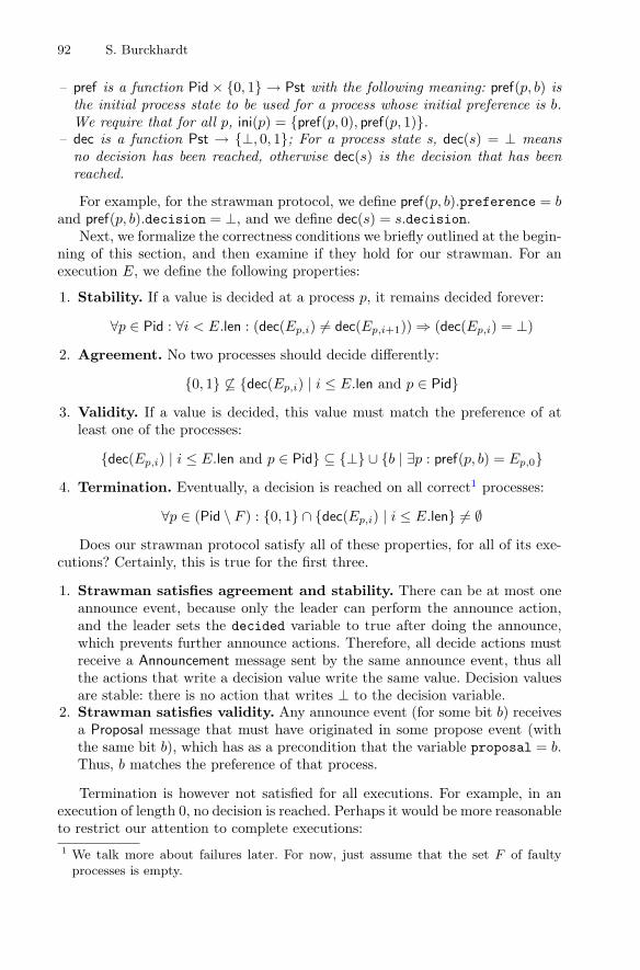
– pref is a function Pid × {0, 1} → Pst with the following meaning: pref(p, b) isthe initial process state to be used for a process whose initial preference is b.We require that for all p, ini(p) = {pref(p, 0), pref(p, 1)}.

– dec is a function Pst → {⊥, 0, 1}; For a process state s, dec(s) = ⊥ meansno decision has been reached, otherwise dec(s) is the decision that has beenreached.

For example, for the strawman protocol, we define pref(p, b).preference = band pref(p, b).decision = ⊥, and we define dec(s) = s.decision.

Next, we formalize the correctness conditions we briefly outlined at the begin-ning of this section, and then examine if they hold for our strawman. For anexecution E, we define the following properties:

1. Stability. If a value is decided at a process p, it remains decided forever:

∀p ∈ Pid : ∀i < E.len : (dec(Ep,i) �= dec(Ep,i+1)) ⇒ (dec(Ep,i) = ⊥)

2. Agreement. No two processes should decide differently:

{0, 1} �⊆ {dec(Ep,i) | i ≤ E.len and p ∈ Pid}3. Validity. If a value is decided, this value must match the preference of at

least one of the processes:

{dec(Ep,i) | i ≤ E.len and p ∈ Pid} ⊆ {⊥} ∪ {b | ∃p : pref(p, b) = Ep,0}4. Termination. Eventually, a decision is reached on all correct1 processes:

∀p ∈ (Pid \ F ) : {0, 1} ∩ {dec(Ep,i) | i ≤ E.len} �= ∅Does our strawman protocol satisfy all of these properties, for all of its exe-

cutions? Certainly, this is true for the first three.

1. Strawman satisfies agreement and stability. There can be at most oneannounce event, because only the leader can perform the announce action,and the leader sets the decided variable to true after doing the announce,which prevents further announce actions. Therefore, all decide actions mustreceive a Announcement message sent by the same announce event, thus allthe actions that write a decision value write the same value. Decision valuesare stable: there is no action that writes ⊥ to the decision variable.

2. Strawman satisfies validity. Any announce event (for some bit b) receivesa Proposal message that must have originated in some propose event (withthe same bit b), which has as a precondition that the variable proposal = b.Thus, b matches the preference of that process.

Termination is however not satisfied for all executions. For example, in anexecution of length 0, no decision is reached. Perhaps it would be more reasonableto restrict our attention to complete executions:1 We talk more about failures later. For now, just assume that the set F of faultyprocesses is empty.


Definition 6. An execution fragment E is complete if it is either infinite orterminated, i.e. if either E.len = ∞, or if no actions are enabled in E.post.

Does the strawman satisfy termination on all complete executions? Theanswer is again no. For example, consider an initial configuration where thepreference of process p is 0. Then we can have an infinite execution

propose(p, 0) propose(p, 0) propose(p, 0) propose(p, 0) . . .

Clearly, no progress is made and an unbounded number of messages is sent.No decision is reached.

Still, it appears that this criticism is not fair! It is hard to imagine howany protocol can achieve termination unless the transport layer and the processscheduler cooperate. Clearly, if the system simply does not deliver messages, ornever executes actions even though they are enabled, nothing good can happen.We need fairness: some assumptions about the “minimal level of service” wemay expect.

Informally, what we want to require is that messages are eventually deliveredunless they become undeliverable, and that spontaneous actions are eventuallyperformed unless they become disabled. We say an action a ∈ Act receives mes-sage m ∈ Msg if rcv(a) = m. We say m ∈ Msg is receivable in a configuration sif there exists an action a that is enabled and that receives m.

Definition 7. A message m is neglected by an execution E if it is receivablein infinitely many configurations, but received by only finitely many actions. Aspontaneous action a is neglected by an execution E, if it is enabled in infinitelymany configurations, but performed only finitely many times.

Definition 8. An execution E of some protocol Φ is fair if it does not neglectany messages or spontaneous actions.

Definition 9. A consensus protocol is a correct consensus protocol if allfair complete executions satisfy stability, agreement, validity, and termination.

Strawman is Correct. We already discussed agreement and validity. Termi-nation is also satisfied for fair executions, for the following reasons. Because thepropose action is always enabled for all p, it must happen at least once (in fact, itwill happen infinitely many times for all p). After it happens just once, announceis now enabled, and remains enabled forever if announce does not happen. Thusannounce must happen (otherwise fairness is violated). But now, for each q,decide is enabled, and thus must happen eventually.

Fair Schedulers. The definition of fairness is purposefully quite general; itdoes not describe how exactly a scheduler is guaranteeing fairness. However, itis useful to consider how to construct a scheduler that guarantees fairness. Oneway to do so is to schedule an action that has maximal seniority, in the sensethat it is executing a spontaneous action or receiving a message that has beenwaiting (i.e. been enabled/receivable but not executed/received) the longest:

94 S. Burckhardt

Definition 10. Let Φ be a protocol, let E be a finite execution of LΦ, and leta ∈ ActΦ be an action that is enabled in post(E). Then, we define the seniorityof a to be the maximal number k such that either (1) some message m in rcv(a)is receivable in E.cnf(E.len−k) but has not been received by any action E.act(j)where E.(E.len−k) < j ≤ E.len, or (2) a is a spontaneous action that is enabledin E.cnf(E.len−k) but is not equal to any E.act(j) where (E.len−k) < j ≤ E.len.

Lemma 1. If a scheduler always picks the most senior enabled action, the result-ing schedule is fair.

Proof. Assume to the contrary that there exists an execution that is not fair,that is, neglects a message or spontaneous action.

First, consider that a message m is neglected. This means that the messageis receivable infinitely often, but received only finitely many times. Considerthe first configuration where it is receivable after the last time it is received, sayE.cnf(k). Since m is receivable in infinitely many configurations {E.cnf(k′) | k′ >k} but never received, there must be infinitely many configurations {E.cnf(k′) |k′ > k} where some enabled action is more senior than the one that receives m(otherwise the scheduler would pick that one). However, an action can only bemore senior than the one that receives m if it is either receiving some messagethat has been waiting (i.e. has been receivable without being received) at least aslong as m, or a spontaneous action that has been waiting (i.e. has been enabledwithout being performed) at least as long as m. But there can only be finitelymany such messages or spontaneous actions, since there are only finitely manyconfigurations {E.cnf(j) | j ≤ k}, and each such configuration has only finitelymany receivable messages and enabled spontaneous actions, by the last conditionin Definition 3; thus we have a contradiction.

Now, consider that a spontaneous action is neglected. We get a contradictionby the same reasoning. ��

Independence. The notion of independence of actions and schedules is alsooften useful. We can define independence for general labeled transition systemsas follows:

Definition 11. Let L = (S, I,Act,→) be a LTS. Two actions a, a′ ∈ L arecalled independent if for all configurations c ∈ Cnf in which both a and a′ areenabled, the following conditions are true:

– They do not disable each other: a is enabled in post(c, a′) and a′ is enabled inpost(c, a).

– Their effect commutes: post(c, a · a′) = post(c, a′ · a).

For protocols, actions performed by different nodes are independent. This isbecause executing an action for process p can only remove messages destinedfor p from the message pool, it can thus not disable any actions on any otherprocess. Actions by different processes always commute, because their effect onthe local state targets local states by different processes, and their effects on themessage pool commute.


We call two schedules s, s′ ∈ Act∗ independent if for all a ∈ s and a′ ∈ s′,a and a′ are independent. Note that if two schedules s, s′ are independent andpossible in some configuration c, then post(c, s · s′) = post(c, s′ · s). Visually, thiscan be seen by doing a typical tiling argument.

2.4 Failures

As we probably all know from experience, failures are common in distributedsystems. Failures can originate in the transport layer (a logical abstraction ofthe network, including switches, links, proxies, etc.) or the nodes (computersrunning the protocol software). Sometimes, the distinction is not that clear (forexample, messages that are waiting in buffers are conceptually in the transportlayer, but are subject to loss if the node fails).

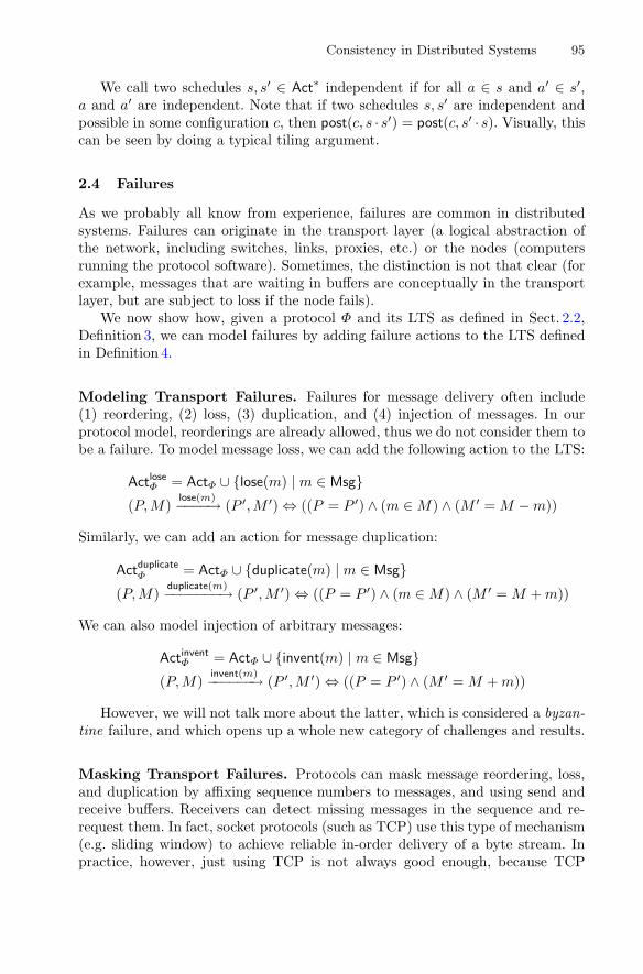
We now show how, given a protocol Φ and its LTS as defined in Sect. 2.2,Definition 3, we can model failures by adding failure actions to the LTS definedin Definition 4.

Modeling Transport Failures. Failures for message delivery often include(1) reordering, (2) loss, (3) duplication, and (4) injection of messages. In ourprotocol model, reorderings are already allowed, thus we do not consider them tobe a failure. To model message loss, we can add the following action to the LTS:

ActloseΦ = ActΦ ∪ {lose(m) | m ∈ Msg}(P,M)

lose(m)−−−−→ (P ′,M ′) ⇔ ((P = P ′) ∧ (m ∈ M) ∧ (M ′ = M − m))

Similarly, we can add an action for message duplication:

ActduplicateΦ = ActΦ ∪ {duplicate(m) | m ∈ Msg}(P,M)

duplicate(m)−−−−−−−→ (P ′,M ′) ⇔ ((P = P ′) ∧ (m ∈ M) ∧ (M ′ = M + m))

We can also model injection of arbitrary messages:

ActinventΦ = ActΦ ∪ {invent(m) | m ∈ Msg}(P,M)

invent(m)−−−−−−→ (P ′,M ′) ⇔ ((P = P ′) ∧ (M ′ = M + m))

However, we will not talk more about the latter, which is considered a byzan-tine failure, and which opens up a whole new category of challenges and results.

Masking Transport Failures. Protocols can mask message reordering, loss,and duplication by affixing sequence numbers to messages, and using send andreceive buffers. Receivers can detect missing messages in the sequence and re-request them. In fact, socket protocols (such as TCP) use this type of mechanism(e.g. sliding window) to achieve reliable in-order delivery of a byte stream. Inpractice, however, just using TCP is not always good enough, because TCP

96 S. Burckhardt

connections can themselves fail. Often, resilience against transport failures needsto be built into the protocol in some form.

A common trick to tolerate message duplication in services is to design theservice calls to be idempotent, meaning that executing a message twice has thesame effect as executing it just once. For example, setting the value of someparameter twice is harmless. Properly written REST protocols use the verbPUT to mark such requests as idempotent, allowing browsers and proxies toduplicate them.

Modeling Node Failures. Typical node failures considered by protocol design-ers are crash failures (a process permanently stops at some point), and crash-recovery failures (a process stops at some point, then recovers later). Sometimes,byzantine failures are also considered, where faulty nodes exhibit arbitrarybehavior, but we are skipping that topic. Typical terminology is to call a processcorrect if it does never experience a crash failure, and if it encounters only finitelymany crash-recovery failures. We let F ⊂ Pid be the subset of faulty processes,i.e. processes that may be incorrect (it is acceptable for processes in F to beactually correct in any given execution).

In a crash failure, the process state is permanently lost, and the process nevertakes another action. In a crash-recovery failure, the process can recover someor all of its state from some form of durable storage (if it cannot, there is littlereason for a process to continue under the same identity). The part of the statethat is lost in crashes is called “soft state”. Often, message buffers are soft state,thus it is possible that messages are lost or duplicated if the crash occurredduring a transition that receives or sends messages.

In asynchronous systems, it is often important to distinguish between silentcrashes and noisy crashes. Silent crashes mean that other processes have no wayto distinguish between a slow response and a crashed process, which can be areal problem as we shall see below. Noisy crashes mean that other processescan use failure detectors to get information about whether a crash occurred.In some situations (e.g. inside a data center), it is often quite feasible to buildfailure detectors, in particular approximate failure detectors, and they can bevery helpful for designing protocols. However, in other situations failure detectionis impossible. For example, if a server loses contact to a JavaScript app runningin somebody’s browser, it does not know if this was a temporary connectionfailure and the app will reconnect at some future time, or if the user has closedthe browser and will never return.

In the following, we consider only silent crash failures. To model them, we usea modified definition of fairness: we allow executions to be ‘unfair’ if this unfair-ness is consistent with processes crashing, in the sense that crashed processesperform no more actions and receive no more messages after they crash.

Definition 12. An execution E of LΦ for some Φ is a complete F -fairexecution if there exists a partial function fails : F → ⊥ ∪ {0 . . . E.len} suchthat


– Crashed processes take no steps after they crash: If fails(p) �= ⊥ for some p,then pid(E.act(j)) �= p for all j > fails(p).

– E is complete: either E.len = ∞, or for all actions a that are enabled inpost(E), fails(pid(a)) �= ⊥.

– E is fair for correct processes: it does not neglect any spontaneous actions aexcept if fails(pid(a)) �= ⊥, and it does not neglect any messages m except iffails(dst(m)) �= ⊥.

2.5 Asynchronous Consensus Under Silent Crash Failuresis Impossible

We now show the famous impossibility result for asynchronous consensus pro-tocols under just 1 silent crash failure, following the same proof structure as inFischer, Lynch and Paterson [7]. Their proof assumes a limited form of protocolwhere for each process, there is exactly one receive action per message, exactlyone spontaneous action, and the actions do not have conditions. We first provethe theorem under the same limitation, and then show how to generalize it tothe more general protocols defined above.

Definition 13. A simple consensus protocol is a consensus protocol

(Pst,Msg,Act, ini, ori, dst, pid, cnd, rcv, snd, upd, pref, dec)

such that the only actions are:

Act = {receive(p,m) | p ∈ Pid,m ∈ Msg} ∪ {run(p) | p ∈ Pid},

and such that:

rcv(receive(p,m)) = m rcv(run(p)) = ⊥ pid(receive(p,m)) = pid(run(p)) = p

and where the actions have no guard:

cnd(receive(p,m)) = cnd(run(p)) = Pst.

Theorem 1. Let Φ be a simple consensus protocol and let Pid contain at leasttwo processes. Then, Φ is not correct in the presence of silent crash failures:in particular, its labeled transition system LΦ = (CnfΦ, IniΦ,ActΦ,→Φ) has acomplete F -fair execution that violates either validity, agreement, stability, ortermination, and where |F | = 1.

Proof. Assume to the contrary that all F -fair executions with |F | ≤ 1 satisfyvalidity, agreement, stability, and termination. We then prove (using a sequenceof lemmas) that a contradiction results.

The key to the proof is the idea of examining the valence of system configu-ration, meaning how many different decisions are possible when starting in thatconfiguration. For a system configuration c ∈ CnfΦ, we define V (c) ⊆ CnfΦ tobe the set of decisions reachable from c:

V (c) = {dec(c′.P (p)) | c′ reachable from c and p ∈ Pid} \ {⊥}

98 S. Burckhardt

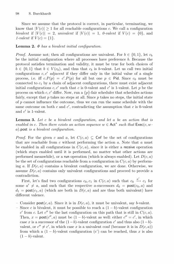
Since we assume that the protocol is correct, in particular, terminating, weknow that |V (c)| ≥ 1 for all reachable configurations c. We call a configurationbivalent if |V (c)| = 2, univalent if |V (c)| = 1, 0-valent if V (c) = {0}, and1-valent if V (c) = {1}.

Lemma 2. Φ has a bivalent initial configuration.

Proof. Assume not; then all configurations are univalent. For b ∈ {0, 1}, let cb

be the initial configuration where all processes have preference b. Because theprotocol satisfies termination and validity, it must be true for both choices ofb ∈ {0, 1} that b ∈ V (cb), and thus that cb is b-valent. Let us call two initialconfigurations c, c′ adjacent if they differ only in the initial value of a singleprocess, i.e. iff c.P (p) = c′.P (p) for all but one p ∈ Pid. Since c0 must beconnected to c1 by a chain of adjacent configurations, there must exist adjacentinitial configurations c, c′ such that c is 0-valent and c′ is 1-valent. Let p be theprocess on which c, c′ differ. Now, run a {p}-fair scheduler that schedules actionsfairly, except that p takes no steps at all. Since p takes no steps, the initial stateof p cannot influence the outcome, thus we can run the same schedule with thesame outcome on both c and c′, contradicting the assumption that c is 0-valentand c′ is 1-valent.

Lemma 3. Let c be a bivalent configuration, and let a be an action that isenabled in c. Then there exists an action sequence w ∈ Act∗ such that Exec(c, w ·a).post is a bivalent configuration.

Proof. For the given c and a, let C(c, a) ⊆ Cnf be the set of configurationsthat are reachable from c without performing the action a. Note that a mustbe enabled in all configurations in C(c, a), since it is either a receive operation(which stays enabled until it is performed, no matter what other actions areperformed meanwhile), or a run operation (which is always enabled). Let D(c, a)be the set of configurations reachable from a configuration in C(c, a) by perform-ing a. If D(c, a) contains a bivalent configuration, we are done. Otherwise, weassume D(c, a) contains only univalent configurations and proceed to provide acontradiction.

First, let’s find two configurations c0, c1 in C(c, a) such that c0a′−→ c1 for

some a′ �= a, and such that the respective a-successors d0 = post(c0, a) andd1 = post(c1, a) (which are both in D(c, a) and are thus both univalent) havedifferent valence.

– Consider post(c, a). Since it is in D(c, a), it must be univalent, say b-valent.– Since c is bivalent, it must be possible to reach a (1 − b)-valent configuration

c′ from c. Let c′′ be the last configuration on this path that is still in C(c, a).Then, x = post(c′′, a) must be (1 − b)-valent as well: either c′′ = c′, in whichcase x is a successor of the (1−b)-valent configuration c′ and thus also (1−b)-valent, or c′′ �= c′, in which case x is a univalent conf (because it is in D(c, a))from which a (1 − b)-valent configuration (c’) can be reached, thus x is also(1 − b)-valent.


– Since we have a path from c to c′′ entirely within C(c, a), and where post(c, a)has different valence than post(c′′, a), there must exist c0, c1 as claimed.

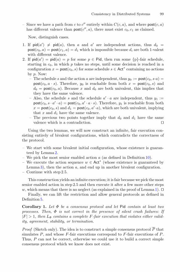
Now, distinguish cases.

1. If pid(a′) �= pid(a), then a and a′ are independent actions, thus d0 =post(c0, a) = post(c1, a) = d1 which is impossible because di are both 1-valentwith different valence.

2. If pid(a′) = pid(a) = p for some p ∈ Pid, then run some {p}-fair schedule,starting in c0, in which p takes no steps, until some decision is reached in aconfiguration x = post(c0, s) for some schedule s ∈ Act∗ containing no actionsby p. Now:– The schedule s and the action a are independent, thus y0 := post(c0, s·a) =

post(c0, a · s). Therefore, y0 is reachable from both x = post(c0, s) andd0 = post(c0, a). Because x and d0 are both univalent, this implies thatthey have the same valence.

– Also, the schedule s and the schedule a′ · a are independent, thus y1 :=post(c0, s · a′ · a) = post(c0, a′ · a · s). Therefore, y1 is reachable from bothx = post(c0, s) and d1 = post(c0, a′ ·a), which are both univalent, implyingthat x and d1 have the same valence.

– The previous two points together imply that d0 and d1 have the samevalence which is a contradiction. ��

Using the two lemmas, we will now construct an infinite, fair execution con-sisting entirely of bivalent configurations, which contradicts the correctness ofthe protocol.

– We start with some bivalent initial configuration, whose existence is guaran-teed by Lemma 2.

– We pick the most senior enabled action a (as defined in Definition 10).– We execute the action sequence w ∈ Act∗ (whose existence is guaranteed by

Lemma 3), then the action a, and end up in another bivalent configuration.– Continue with step 2.5.

This construction yields an infinite execution; it is fair because we pick the mostsenior enabled action in step 2.5 and then execute it after a few more other stepsw, which means that there is no neglect (as explained in the proof of Lemma 1). ��

Finally, we can lift the restriction and allow general protocols as defined inDefinition 5.

Corollary 1. Let Φ be a consensus protocol and let Pid contain at least twoprocesses. Then, Φ is not correct in the presence of silent crash failures: If|F | > 1, then LΦ contains a complete F -fair execution that violates either valid-ity, agreement, stability, or termination.

Proof (Sketch only). The idea is to construct a simple consensus protocol P thatsimulates P , and whose F -fair executions correspond to F -fair executions of P .Thus, P can not be correct, otherwise we could use it to build a correct simpleconsensus protocol which we know does not exist.

100 S. Burckhardt

The messages are the same (Msg = Msg). The local state Pst stores (1) theprocess state Pst, (2) an “inbox”, i.e. a multiset representing messages that areavailable, and (3) a step counter recording how many times this process has takena step, and (4) a data structure recording the timestamps (i.e. step counts) formessages in Msg and spontaneous actions in Act, used to calculate the seniorityof actions as defined in Definition 10. On receive(p,m), the received message issimply added to the inbox. On run(p), we look for the most senior action, andexecute it.

The key requirement is that for every fair execution E of P we find a cor-responding fair execution E of P . Consider a message m: if it does not getneglected in E, it must be received, meaning that it reaches the inbox; andbecause run(dst(m)) does not get neglected in E, it executes infinitely manytimes. Because the scheduler that is simulated by run is fair, as shown byLemma 1, the simulated execution is fair as well. ��

Ways Around Impossibility. Impossibility results are often called negativeresults, but in fact, they usually help us to discover new ways in which to changeour approach or our definitions, in order to succeed. There are many ways towork around the impossibility result we just proved:

– The result applies only to asynchronous systems. We can solve consensus insynchronous systems, e.g. if we have some bounds on message delays.

– The result assumes that crashes are silent. We can solve consensus if we havefailure detectors (for an extensive list of various consensus algorithms, see [5]).

– The result assumes an adversarial scheduler: this means that our proof con-structs an extremely contrived schedule to prove nontermination.

The last item is perhaps the most interesting. In the next section, we showan asynchronous protocol for consensus that can be tuned to terminate quiteefficiently in practice.

2.6 The PAXOS Protocol

We now have a closer look at the PAXOS protocol for asynchronous consensusby Leslie Lamport [11]. It is a standard mechanism to provide fault tolerancein distributed systems, and variations of the classic protocol are used in manypractical systems, e.g. in the Chubby lock service [4] or in Zookeeper [9].

The basic idea is to perform a leader-based consensus: a leader p performs avoting round (whose goal is to reach consensus on a bit) by sending a proposalfor a consensus value to all participants, and if p gets a majority to agree withthe proposal, p informs all participant about the winning value. Voting roundscan fail for various reasons, but a leader can always start a new round, whichcan still succeed (i.e. the protocol never gets stuck with no chance of success).

The trick is to (1) design the protocol to satisfy agreement, validity, andstability even if there are many competing leaders, and (2) make it unlikely


types| Round = (N0 × Pid) using lexicographic order| Vote = (Round × {0, 1}) using lexicographic order

process state| state : {N, Q, P} initially N (leader)| inbox : P(Msg) initially ∅ (leader)| lasttried : N0 initially 0 (leader)| quorum : P(Pida) initially ∅ (leader)| lastpromise : Round initially (0, pid) (acceptor)| lastvote : Vote initially ((0, pid), bpid) for bpid ∈ {0, 1} (acceptor)| decision : {⊥, 0, 1} initially ⊥ (learner)

messages| Inquiry(n : N, p : Pidl, q : Pida) //sent from leader p to acceptor q| LastVote(n : N, p : Pidl, q : Pida, v : Vote) //sent from acceptor q to leader p| Proposal(n : N, p : Pidl, q : Pida, b : {0, 1}) //sent from leader p to acceptor q| Vote(n : N, p : Pidl, q : Pida, b : {0, 1}) //sent from acceptor q to leader p| Winner(p : Pidl, q : Pidr, b : {0, 1}) //sent from leader p to learner q

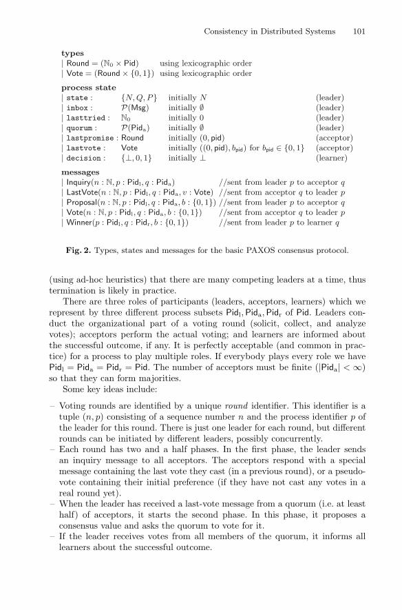
Fig. 2. Types, states and messages for the basic PAXOS consensus protocol.

(using ad-hoc heuristics) that there are many competing leaders at a time, thustermination is likely in practice.

There are three roles of participants (leaders, acceptors, learners) which werepresent by three different process subsets Pidl,Pida,Pidr of Pid. Leaders con-duct the organizational part of a voting round (solicit, collect, and analyzevotes); acceptors perform the actual voting; and learners are informed aboutthe successful outcome, if any. It is perfectly acceptable (and common in prac-tice) for a process to play multiple roles. If everybody plays every role we havePidl = Pida = Pidr = Pid. The number of acceptors must be finite (|Pida| < ∞)so that they can form majorities.

Some key ideas include:

– Voting rounds are identified by a unique round identifier. This identifier is atuple (n, p) consisting of a sequence number n and the process identifier p ofthe leader for this round. There is just one leader for each round, but differentrounds can be initiated by different leaders, possibly concurrently.

– Each round has two and a half phases. In the first phase, the leader sendsan inquiry message to all acceptors. The acceptors respond with a specialmessage containing the last vote they cast (in a previous round), or a pseudo-vote containing their initial preference (if they have not cast any votes in areal round yet).

– When the leader has received a last-vote message from a quorum (i.e. at leasthalf) of acceptors, it starts the second phase. In this phase, it proposes aconsensus value and asks the quorum to vote for it.

– If the leader receives votes from all members of the quorum, it informs alllearners about the successful outcome.

102 S. Burckhardt

action answer(n : N, p : Pidl, q : Pida, v : Vote) at q (acceptor)| receives Inquiry(n, p, q)| condition (lastpromise < (n, p)) ∧ (lastvote = v)| sends LastVote(n, p, q, v)| updates lastpromise ← (n, p)

action accept(n : N, p : Pidl, q : Pida, b : {0, 1}) at q (acceptor)| receives Proposal(n, p, b)| condition lastpromise = (n, p)| sends Vote(n, p, q, b)| updates lastvote ← ((n, p), b)

action learn(q : Pidr, b : {0, 1}) at q (learner)| receives Winner(p, q, b)| updates decision ← b

Fig. 3. The acceptor actions and the one learner actions for the basic PAXOS consensusprotocol.

action inquire(n : N, p : Pidl) at p (leader)| condition (state = N) ∧ (n = lasttried+ 1)| sends ∑

q∈PidaInquiry(n, p, q)

| updates state ← Q; lasttried ← n

action propose(n : N, p : Pidl, b : {0, 1}, Q : P(Pida), lv : Q → Vote) at p (leader)| condition inbox ≥ ∑

q∈Q LastVote(n, p, q, lv(q))| condition (state = Q) ∧ (lasttried = n) ∧ (|Q| > |Pida|/2)| condition max{lv(q) | q ∈ Q} = ( , b)| sends ∑

q∈Q Proposal(n, p, q, b)

| updates state ← P ; quorum ← Q; inbox ← ∅action announce(n : N, p : Pidl, b : {0, 1}, Q : P(Pida)) at p (leader)| condition inbox ≥ ∑

q∈Q Vote(n, p, q, b)

| condition (state = P ) ∧ (lasttried = n) ∧ (quorum = Q)| sends ∑

q∈PidrWinner(p, q, b)

| updates state ← N ; inbox ← ∅action receive(m : Msg) at dst(m) (leader)| receives m| updates inbox ← inbox+ m

action abandon(n : N, p : Pidl) at p (leader)| condition (lasttried = n) ∧ (state ∈ {P, V })| updates state ← N ; inbox ← ∅

Fig. 4. The leader actions for the basic PAXOS consensus protocol.

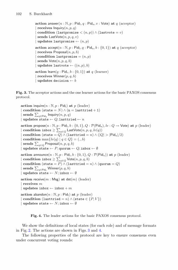
We show the definitions of local states (for each role) and of message formatsin Fig. 2. The actions are shown in Figs. 3 and 4.

The following properties of the protocol are key to ensure consensus evenunder concurrent voting rounds:


– Rounds are totally ordered (lexicographically based on the order, then theprocess id). Participants are no longer allowed to participate in a lower roundonce they are participating in a higher round.

– When transitioning from the first phase (gather last vote messages) to thesecond phase (send out proposal messages), the leader chooses the consensusvalue belonging to the highest vote among all the last-vote messages. Thisensures that if a prior round was actually successful (i.e. it garnered a majorityof votes), the new round uses the same bit value.

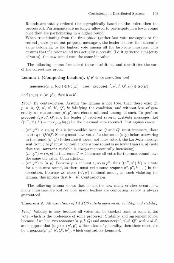
The following lemma formalized these intuititons, and constitutes the coreof the correctness proof.

Lemma 4 (Competing Leaders). If E is an execution and

announce(n, p, b,Q) ∈ trc(E) and propose(n′, p′, b′, Q′, lv) ∈ trc(E),

and (n, p) < (n′, p′), then b = b′.

Proof. By contradiction. Assume the lemma is not true, then there exist E,p, n, b, Q, p′, n′, b′, Q′, lv falsifying the condition, and without loss of gen-erality we can assume (n′, p′) are chosen minimal among all such. To performpropose(n′, p′, b′, Q′, lv), the leader p′ received several LastVote messages; Let((n′′, p′′), b′) = maxq∈Q lv(q) be the maximal vote received. Distinguish cases:

– (n′′, p′′) < (n, p) this is impossible: because Q and Q′ must intersect, thereexists q ∈ Q∩Q′. Since q must have voted for the round (n, p) before answeringin the round (n′, p′) (otherwise it would not have voted), the LastVote messagesent from q to p′ must contain a vote whose round is no lower than (n, p) (notethat the lastvote variable is always monotonically increasing).

– (n′′, p′′) = (n, p) in that case, b′ = b because all votes for the same round havethe same bit value. Contradiction.

– (n′′, p′′) > (n, p). Because p is at least 1, so is p′′, thus ((n′′, p′′), b′) is a votefor a non-zero round, so there must exist some propose(n′′, p′′, b′, , ) in theexecution. Because we chose (n′, p′) minimal among all such violating thelemma, this implies that b = b′. Contradiction.

The following lemma shows that no matter how many crashes occur, howmany messages are lost, or how many leaders are competing, safety is alwaysguaranteed.

Theorem 2. All executions of PAXOS satisfy agreement, validity, and stability.

Proof. Validity is easy because all votes can be tracked back to some initialvote, which is the preference of some processor. Stability and agreement followbecause if we had two announce(n, p, b,Q) and announce(n′, p′, b′, Q′) with b �= b′,and suppose that (n, p) < (n′, p′) without loss of generality, then there must alsobe a propose(n′, p′, b′, Q′, lv ′), which contradicts Lemma 4.

104 S. Burckhardt

Of course, termination is not possible for arbitrary fair schedules in the pres-ence of failures because of Theorem 1. However, the following property holds: suc-cess always remains possible as long as there remains some non-crashed leader,some non-crashed learner, and at least �|Pida/2|� non-crashed acceptors. Thereason is that:

– A leader cannot get stuck in any state: if it is waiting for something (suchas the receipt of some message), and that something is not happening (forexample, due to a crash), the leader can perform the spontaneous actionabandon to return to a neutral state, from which it can start a new, higherround.

– If a leader p starts a new round (n, p) that is larger than any previousrounds, and if no other leaders are starting even higher rounds, and if atleast �|Pida/2|� acceptors remain, and if there are no more crashes, then theround succeeds.

The PAXOS algorithm shown, and the correctness proof, are both based onthe original paper by Lamport [11]. Since then, there have been many morepapers on the subject, and many alternative (e.g. disk-based) and optimized(e.g. for solving continuous consecutive consensus problems) versions of PAXOSexist.

3 Strong Consistency and CAP

In this section we examine how to understand the consistency of shared data. Weexplore the cost of strong consistency (in terms of reliability or performance). Wedevelop abstractions that help system implementors to articulate the consistencyguarantees they are providing to programmers.

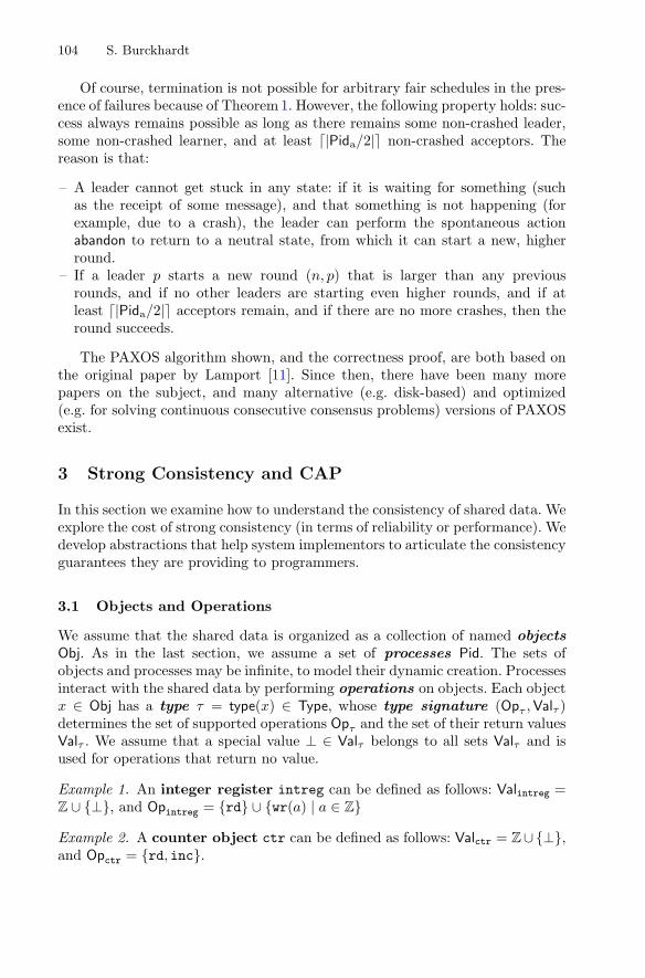
3.1 Objects and Operations

We assume that the shared data is organized as a collection of named objectsObj. As in the last section, we assume a set of processes Pid. The sets ofobjects and processes may be infinite, to model their dynamic creation. Processesinteract with the shared data by performing operations on objects. Each objectx ∈ Obj has a type τ = type(x) ∈ Type, whose type signature (Opτ ,Valτ )determines the set of supported operations Opτ and the set of their return valuesValτ . We assume that a special value ⊥ ∈ Valτ belongs to all sets Valτ and isused for operations that return no value.

Example 1. An integer register intreg can be defined as follows: Valintreg =Z ∪ {⊥}, and Opintreg = {rd} ∪ {wr(a) | a ∈ Z}Example 2. A counter object ctr can be defined as follows: Valctr = Z∪{⊥},and Opctr = {rd, inc}.


Sequential Semantics. The type of an object, as defined above, does notactually describe the semantics of the operation, only their syntax. We formallyspecify the sequential semantics of a data type τ by a function

Sτ : Opτ × Op∗τ → Valτ ,

which, given an operation and sequence of prior operations, specifies the expectedreturn value. For a register, read operations return the value of the last precedingwrite, or zero if there is no prior write. For a counter, read operations return thenumber of preceding increments. Thus, for any sequence of operations ξ:

Sintreg(rd, ξ) = a, if wr(0) ξ = ξ1 wr(a) ξ2 andξ2does not contain wr operations;

Sctr(rd, ξ) = (the number of inc operations in ξ);

Our definition of the sequential semantics uses sequences of prior operations(representing all earlier updates), rather than the current state of an object,to define the behavior of reads. This choice is useful: for many implementa-tions, there are multiple versions of the state, and these versions are often bestunderstood as the result of using various update sequences (such as logs), sub-sequences, or segments.

Moreover, for objects such as the integer register, only the last update mat-ters, since it overwrites completely all information in the object. For the counter,however, all updates matter. Similarly, if considering objects that have multiplefields and support partial updates, e.g. updates that modify individual fields, itis not enough to look at the last update to determine the current state of theobject.

In general, operations may both read and modify the state. Operations thatreturn no value are called update-only operations. Similarly, we call an operationo of a type τ read-only if it has no side effect, i.e. if for all o′ ∈ Opτ and u, v ∈ Op∗

τ ,we have Sτ (o′, u · o · v) = Sτ (o′, u · v).

What is an Object? There is often some ambiguity to the question of whatwe should consider to be an object. For example, consider a cloud table storageAPI that provides tables that store records (consisting of several fields that havevalues) indexed by keys. Then:

– We can consider each record to be an object, named by the combination of thetable name and the key, and supporting operations for reading and writingfields or removing the object.

– We can consider the whole table to be an object, named by the table name.Operations specify the key (and the field, if accessing individual fields).

– We can consider each field to be an object, named by the combination of thetable name, the key, and the field name. This approach seems most consistentwith the types shown above (integer registers, counters).

– We can consider the entire storage to be a single object, and have operationsto target a specific (table, key, field) combination.

106 S. Burckhardt

We propose the following definition, or perhaps we should say guideline:

– An object is the largest unit of data that can be written atomically withoutusing transactions.

– A transactional domain is the largest unit of data that can be written atomi-cally by using transactions.

Traditional databases follow a philosophy without objects (nothing can bewritten outside of a transaction) and large transactional domains (the entiredatabase), which requires strong transaction support. Cloud storage and webprogramming rely more commonly on moderately to large sized objects, andtransactional domains that do not contain all data (transaction support is typ-ically nonexistent, or at best limited). The reason is that the latter approachis easier to guarantee as a scalable service. Unfortunately, it is also harder toprogram.

3.2 Strong Consistency

Intuitively, programmers expect operations on shared data to be linearizable.Informally, this means that when they call into some API to read or write ashared value, they expect a behavior that is consistent with (i.e. observationallyundistinguishable from):

– a single copy of the shared data being maintained somewhere.– the read or write operations being applied to that copy somewhere in between

the call and the return.

Unfortunately, guaranteeing these conditions can be a performance and relia-bility problem, if communication between processes is expensive and/or unavail-able. Many systems thus relax the consistency. A good test to see whether asystem is indeed linearizable (in fact, sequentially consistent) is shown in Fig. 5.On an linearizable or sequentially consistent system, when running programsA and B (one time each), there is at most one winner. Why? Informally, itis because under sequential consistency, all operations are organized into someglobal sequence. In this case, it means that the two writes must happen in someorder — we don’t know which one, but the system will decide on one or theother, which implies that either A or B (or both) do not win:

– If the system decides that A’s write to x happens before B’s write to y, thenit must also happen before B’s read from x, thus the value read must be 1, soB does not win.

– If the system decides that B’s write to y happens before A’s write to x, thenit must also happen before A’s read from y, thus the value read must be 1, soA does not win.

This reasoning seems still a bit informal - talking about ‘happens before’without a solid foundation can get quite confusing. In order to give a more rig-orous reasoning, we first need a precise definition of what sequential consistencyand linearizability mean.


Program (A)

| x.wr(1); //a1

| if (y.rd = 0) //a2

| | print “A wins”;

Program (B)

| y.wr(1); //b1| if (x.rd = 0) //b2| | print “B wins”;

Fig. 5. The Dekker Litmus test, using two integer registers x, y (which are initially 0).If we run these two concurrently on a sequentially consistent or linearizable system,there is at most one winner.

Abstract Executions. To specify consistency models, we use abstract execu-tions. The basic idea is very simple:

1. A consistency model is formalized as a set of abstract executions, whichare mathematical structures (visualized using graphs) consisting of opera-tion events (vertices) and relations (edges), subject to conditions. Abstractexecutions capture “the essence” of an execution (that is, what operationsoccurred, and how those operations are related), without including low-leveldetails (such as exactly what messages were sent when and where).

2. We describe what it means for a concrete execution of a system to correspondto an abstract execution.

3. We say that a system is correct if all of its concrete executions correspondto some abstract execution of the consistency model.

The advantage of this approach is that we can separately (1) determinewhether programs are correct for a given consistency model, without needingto know details about the system architecture, and (2) determine whether a sys-tem correctly implements some consistency model, without knowing anythingabout the program that is running on it. Consistency models can be thought ofas a contract between the programmer and the system implementor.

For sequential consistency, we define abstract executions in two steps. First,we define operation graphs.

Definition 14. An operation graph is a tuple (Evt, pid, obj, op, rval, po) where

– Evt is a set of events.– pid : Evt → Pid describes the process on which the event happened.– po ⊆ Evt×Evt is a partial order (called process order) that describes the order

in which events happened on each process. We require that po is a union oftotal orders for each process, that is, there exist for each p ∈ Pid a total orderpop ⊆ (pid−1(p) × pid−1(p)) such that po is their union: po =

⋃p∈Pid pop.

– obj, op, rval are event attributes (i.e. functions Evt) describing the details ofthe operation: each event e ∈ Evt represents an operation op(e) ∈ Optype(obj(e))on an object obj(e) ∈ Obj, which returns the value rval(e) ∈ Valtype(obj(e)).

Operation graphs capture the relevant interactions between the system andthe client program. However, they do not explain the underlying reasons. Look-ing just at the operation graph, it can be difficult to determine the order in

108 S. Burckhardt

which the system processed operations. Abstract executions contain this addi-tional information: in the case of sequential consistency, a total order over alloperations:

Definition 15. Define the set ASC of sequentially consistent abstract executionsto consist of all tuples(Evt, pid, obj, op, rval, po, to), where

– (Evt, . . . , po) is an operation graph.– to ⊆ Evt × Evt is a total order.– to is consistent with process order: po ⊆ to.– The return value of each operation matches the sequential specification Sτ (as

defined in Sect. 3.1), applied to the sequence of to-prior operations:

∀e ∈ Evt : rval(e) = Stype(obj(e))(op(e), (to−1(e) ∩ obj−1(obj(e))).sort(to))

In pictures, we usually draw abstract executions by (1) creating a vertex foreach event, and aligning events into columns corresponding to process identifiers,and (2) adding arrows to represent to ordering edges.

We can now define sequential consistency; note that we purposefully omita precise definition of what a concrete execution is, but simply assume thatit contains operation events that can be meaningfully related to the abstractexecution.

Definition 16. A concrete execution of some system is sequentially consistentif there exists an abstract sequentially consistent execution, with correspondingoperation events, process order, and attributes.

Dekker Explanation. We can now explain why under sequential consistency,there can never be two winners in the Dekker litmus test (Fig. 5). Suppose therewere two winners. This would mean that in the corresponding abstract execu-tion, there are four events {a1, a2, b1, b2} (meaning that pid(a1) = pid(a2) = a,pid(b1) = pid(b2) = b, obj(a1) = obj(b2) = x, obj(b1) = obj(a2) = y,op(a1) = op(b1) = wr(1), op(a2) = op(b2) = rd, rval(a2) = rval(b2) = 0, andpo = {(a1, a2), (b1, b2)}).

Now we can argue that there is no way to construct to without creating acycle and thus a contradiction:

– Because rval(a2) = 0, it cannot be the case that b1to−→ a2 (because that would

imply a return value of 1). Therefore, because to is a total order, a2to−→ b1.

– Because rval(b2) = 0, it cannot be the case that a1to−→ b2 (because that would

imply a return value of 1). Therefore, because to is a total order, b2to−→ a1.

– Because po ⊆ to, a1to−→ a2 and b1

to−→ b2.

Linearizability. Sometimes, systems use a slightly stronger consistency modelthan sequential consistency, called linearizability. The difference is that for lin-earizability, we additionally require that the order to must not contradict theorder of operation calls and operation returns in the concrete execution.


Definition 17. A concrete execution of some system is linearizable if thereexists a corresponding abstract sequentially consistent execution, such that forany two operations e, e′ ∈ Evt in the abstract execution satisfying e

to−→ e′, it isnot the case that return(e′) < call(e) in the concrete execution.

Note that any linearizable concrete execution is also sequentially consistent.The converse is not true in general; we will show an example in the next section.

There is an alternative popular interpretation of linearizability that roughlygoes as follows: The abstract execution must be consistent with a placementof commit events of operations, which are placed somewhere in between calland return. The two definitions are equivalent: (1) if the order matches commitevents, then it cannot violate the condition above, and (2) if the condition aboveis not violated, we can find a commit event placement.

3.3 CAP Theorem

The CAP theorem explores tradeoffs between Consistency, Availability, andPartition tolerance, and concludes that, while it is possible to provide any twoof these properties, it is impossible to provide all three. It was conjectured byBrewer [1] and proved by Gilbert and Lynch [8]. Our proof here follows thesame simple reasoning as the one by Gilbert and Lynch, but we use sequentialconsistency instead of linearizability.

We use the following meaning of the three terms. Consistency means sequen-tial consistency as defined above. Availability means that all operations onobjects eventually complete. Partition Tolerance means that the system keepsoperating even if the network becomes permanently partitioned, i.e. if there existsa subset of isolated processes Iso ⊆ Pid such that the processes in Iso and theprocesses in Pid \ Iso cannot communicate in any way.

Theorem 3 (CAP). No system with at least two processes can provide sequen-tial consistency, availability, and partition tolerance.

Proof. Assume such a system exists. Consider two processes a, b ∈ Pid and apermanent network partition Iso = {a} that isolates process a. We run threeindependent experiments, called A, B, and AB. In experiment A, process a runsthe program (A) shown in Fig. 5, while process b does nothing. In experiment B,process b runs the program (B) shown in Fig. 5, while process a does nothing.In experiment AB, both processes run the respective program. Then:

– In experiment A, availability and partition tolerance imply that the codeexecutes to completion. Consistency means that process a prints “A wins”(because there is only one process accessing the data, the semantics is equiv-alent to standard sequential semantics).

– There is no way for process a to distinguish between experiments A and AB,thus it must print “A wins” in experiment AB as well.

– For the symmetric reason, process b must print “B wins” in experiment AB.

110 S. Burckhardt

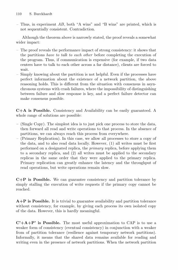
– Thus, in experiment AB, both “A wins” and “B wins” are printed, which isnot sequentially consistent. Contradiction.

Although the theorem above is narrowly stated, the proof reveals a somewhatwider impact:

– The proof reveals the performance impact of strong consistency: it shows thatthe partitions have to talk to each other before completing the execution ofthe program. Thus, if communication is expensive (for example, if two datacenters have to talk to each other across a far distance), clients are forced towait.

– Simply knowing about the partition is not helpful. Even if the processes haveperfect information about the existence of a network partition, the abovereasoning holds. This is different from the situation with consensus in asyn-chronous systems with crash failures, where the impossibility of distinguishingbetween failure and slow response is key, and a perfect failure detector canmake consensus possible.

C+A is Possible. Consistency and Availability can be easily guaranteed. Awhole range of solutions are possible:

– (Single Copy). The simplest idea is to just pick one process to store the data,then forward all read and write operations to that process. In the absence ofpartitions, we can always reach this process from everywhere.

– (Primary Replication). In this case, we allow all processes to store a copy ofthe data, and to also read data locally. However, (1) all writes must be firstperformed on a designated replica, the primary replica, before applying themto a secondary replica, and (2) all writes must be applied to the secondaryreplicas in the same order that they were applied to the primary replica.Primary replication can greatly enhance the latency and the throughput ofread operations, but write operations remain slow.

C+P is Possible. We can guarantee consistency and partition tolerance bysimply stalling the execution of write requests if the primary copy cannot bereached.

A+P is Possible. It is trivial to guarantee availability and partition tolerancewithout consistency, for example, by giving each process its own isolated copyof the data. However, this is hardly meaningful.

C’+A+P’ is Possible. The most useful approximation to CAP is to use aweaker form of consistency (eventual consistency) in conjunction with a weakerfrom of partition tolerance (resilience against temporary network partitions).Informally, it means that the shared data remains available for reading andwriting even in the presence of network partitions. When the network partition


heals, processes reconcile conflicting updates that happened during the networkpartition, and converge to a common state. Understanding specifications andimplementations of eventual consistency is the main topic for the remainder ofthis course.

4 Eventual Consistency Models and Mechanisms

Weakening the consistency guarantees can improve performance and availability,but it can also create problems for unaware programmers. Understanding exactlywhat can go wrong, and how to write programs that are resilient, remains animportant challenge. One of the key difficulties is that there are many subtlevariations of consistency models, and myriads of architectures and optimizationsthat all have slightly different effects. We study this problem by approaching itfrom two sides:

– In Sect. 4.1, we show how to generalize sequentially consistent abstract exe-cutions to eventually consistent abstract executions, and show how to expressvarious guarantees (causality, consistent prefix, read my writes, monotonicreads) and combinations of guarantees.

– In Sect. 4.2, we take a closer look at a few selected architectures that imple-ment some form of consistency, and show how to specify their behavior usingabstract executions.

4.1 Eventual Consistency Models

The following simple definition of quiescent consistency is often used to describeeventually consistent systems:

if clients stop issuing update requests, then the replicas will eventuallyreach a consistent state.

However, quiescent consistency is very weak. For example, it (1) does notspecify what happens if clients never stop issuing updates, which is commonin reactive systems such as services, and (2) does not in any way restrict theintermediate values. Few programs will work correctly under quiescent consis-tency, and most architectures provide much stronger guarantees. Thus, we needa better way to define eventual consistency models.

To devise a better model for eventual consistency, we start by deconstructingour definition of sequential consistency (Definition 15). In that definition, we usea total order to to figure out what value an operation e on some object x = obj(e)should return:

∀e ∈ Evt : rval(e) = Stype(x)(op(e), (to−1(e) ∩ obj−1(x)).sort(to)) (1)

The key observation is that the total order to is playing two independentroles:

112 S. Burckhardt

1. It is used to determine what prior operations are visible to e. In (1), this isthe part to−1(e), which returns the set of all operations e′ such that e′ to−→ e.

2. It is used to arbitrate between conflicting operations. In (1), this is the partsort(to): it ensures that everyone is using the same order to sort conflictingoperations (e.g. multiple writes to the same location).

Definition 18. Given a type τ , we say two operations o1, o2 ∈ Opτ are write-conflicting if there exists an operation o ∈ Opτ and operation sequences u,w ∈Op∗

τ such that Sτ (o, u · o1 · o2 ·w) �= Sτ (o, u · o2 · o1 ·w). Given an operation graph(Evt, . . . , obj, op, . . . ), we say that two events e1, e2 ∈ Evt are write-conflicting(written as wconflict(e1, e2)) if (1) obj(e1) = obj(e2), and (2) op(e1) and op(e2)are write-conflicting.

We now define eventually consistent abstract executions, similar to(Definition 15), but using two separate relations; a visibility relation is usedto determine what operations are visible, and an arbitration order is used todetermine how to order conflicting operations.

Definition 19. Define the set AEC of eventually consistent abstractexecutions to consist of all tuples (Evt, pid, obj, op, rval, po, vis, ar), where

1. (Evt, . . . , po) is an operation graph.2. The visibility relation vis ⊆ Evt × Evt is an acyclic, irreflexive relation.3. Operations become eventually visible: for all e ∈ Evt, e

vis−→ e′ for almost alle′ ∈ Evt (i.e. all but finitely many).

4. The arbitration order ar ⊆ Evt × Evt is a partial order.5. The arbitration order orders all conflicting operations that are visible to

another operation: for all e1, e2, e ∈ Evt:

((e1vis−→ e) ∧ (e2

vis−→ e) ∧ wconflict(e1, e2)) ⇒ ((e1ar−→ e2) ∨ (e2

ar−→ e1))

6. There are no causal cycles: po ∪ vis is acyclic.7. The return value of each operation matches the sequential specification Sτ

applied to visible operations in arbitration order:

∀e ∈ Evt : rval(e) = Stype(obj(e))(op(e), (vis−1(e) ∩ obj−1(obj(e))).sort(ar))

Note how the return value is determined in condition 7: first, it determinesthe set of visible events on the same object vis−1(e) ∩ obj−1(obj(e)), then itsorts this set into a sequence using ar, and then applies the sequential semantics.Although the sorting is not quite deterministic (since ar is not necessarily a totalorder), the value of the whole expression is deterministic because condition 5ensures that ar determines at least the order of write-conflicting operations.

For an abstract eventually consistent execution A, we define the happens-before order hbA, sometimes also called the causal order, to be the partial orderhbA = (A.po ∪ A.vis)+ (note that we rely on the acyclicity guaranteed by con-dition 6). The happens-before order tracks potential causal dependency chains:


if two operations are issued by the same process (apo−→ b), or if the first operation

is visible to the second (a vis−→ b), the second may causally depend on the first.How do these concepts map into practical implementations? Consider a typ-

ical implementation where each process maintains a replica of the shared state.Updates performed on a replica are broadcast to other replicas in some way.Visibility and arbitration are often determined in one of the following ways:

– Arbitration is typically determined either by (1) some timestamp, or (2) theorder in which updates are processed on some primary replica.

– Visibility is typically determined by two factors, (1) the timing of when aprocess learns about an update (a process learns about a local update imme-diately, and about a remote update when it receives a message), and (2) thetime at which a process chooses to make that update visible to subsequentqueries (which could be as soon as it learns about it, or delayed, for exampleuntil an update is confirmed by the primary replica).

Eventual consistency is much stronger than quiescent consistency, but stillquite weak. Most of the time, systems guarantee additional properties. In par-ticular, the following guarantees are common. We start with a table giving theformal definition, and explain them below. These guarantees are not mutuallyexclusive; quite to the contrary, most systems provide a combination.

Guarantee Condition

Sequential consistency| vis = ar

Read my writes po ⊆ vis

Consistent prefix ar is total, and ∀e : ∃e′ : vis−1(e) = ar−1(e′)

Monotonic reads (vis; po) ⊆ vis

Causal visibility hb ⊆ vis

Causal arbitration hb ⊆ ar

Sequential Consistency. We already defined this in the last section. Formally,sequential consistency means that arbitration and visibility are one and thesame.

Read My Writes. If the same process performs two operations, it may expectthat the first operation is visible to the second. For example, if we incrementand then read a counter on the same process, read-my-writes guarantees thatthe read does not return zero.

Consistent Prefix. Sometimes it is acceptable to read a stale value, as long asthat value appears as a past value of some timeline of values that everyoneagrees on. Consistent prefix means just that: (1) a timeline is maintained(ar is a total order), and (2) the visible updates for any event e match someprefix of ar.

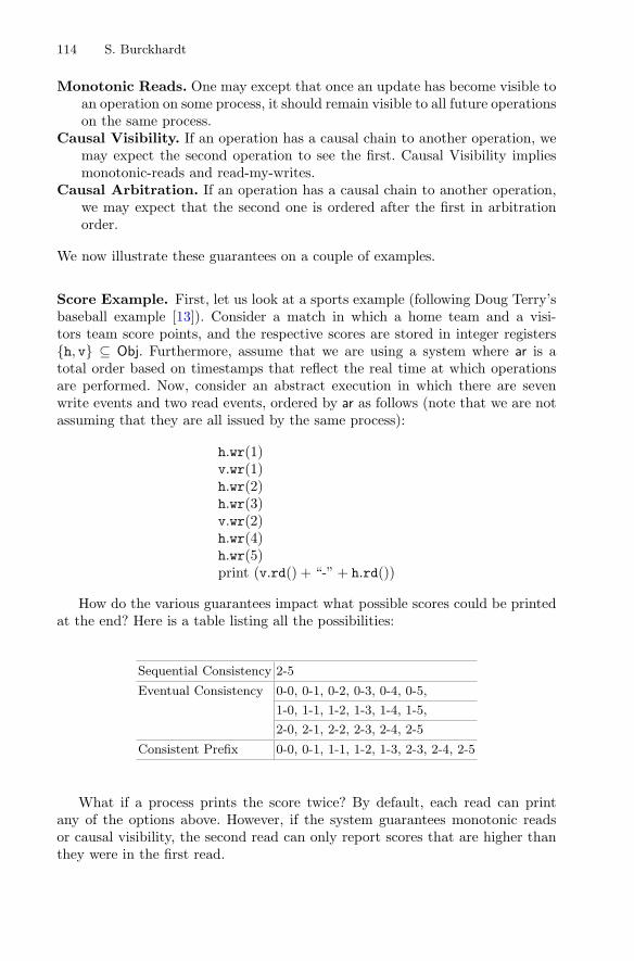
114 S. Burckhardt

Monotonic Reads. One may except that once an update has become visible toan operation on some process, it should remain visible to all future operationson the same process.

Causal Visibility. If an operation has a causal chain to another operation, wemay expect the second operation to see the first. Causal Visibility impliesmonotonic-reads and read-my-writes.

Causal Arbitration. If an operation has a causal chain to another operation,we may expect that the second one is ordered after the first in arbitrationorder.

We now illustrate these guarantees on a couple of examples.

Score Example. First, let us look at a sports example (following Doug Terry’sbaseball example [13]). Consider a match in which a home team and a visi-tors team score points, and the respective scores are stored in integer registers{h, v} ⊆ Obj. Furthermore, assume that we are using a system where ar is atotal order based on timestamps that reflect the real time at which operationsare performed. Now, consider an abstract execution in which there are sevenwrite events and two read events, ordered by ar as follows (note that we are notassuming that they are all issued by the same process):

h.wr(1)v.wr(1)h.wr(2)h.wr(3)v.wr(2)h.wr(4)h.wr(5)print (v.rd() + “-” + h.rd())

How do the various guarantees impact what possible scores could be printedat the end? Here is a table listing all the possibilities:

Sequential Consistency 2-5

Eventual Consistency 0-0, 0-1, 0-2, 0-3, 0-4, 0-5,

1-0, 1-1, 1-2, 1-3, 1-4, 1-5,

2-0, 2-1, 2-2, 2-3, 2-4, 2-5

Consistent Prefix 0-0, 0-1, 1-1, 1-2, 1-3, 2-3, 2-4, 2-5

What if a process prints the score twice? By default, each read can printany of the options above. However, if the system guarantees monotonic readsor causal visibility, the second read can only report scores that are higher thanthey were in the first read.


Causality Example. Not all systems guarantee causal arbitration or causalvisibility. This can lead to odd behaviors. For example, consider a chat applica-tion where participants {Alice,Bob,Carol} ⊆ Pid append to a list (the “wall”),or read the list. Alice asks a question, and Bob sees it and answers it. Finally,Carol looks at the chat and sees Bob’s answer. But what about Alice’s question?

Alice Bob Carol

e1: wall.append(“Anyone?”) e2: print wall.rd e4: print wall.rd

e3: wall.append(“Bob here.”)

Since Bob saw Alice’s question, we know e1vis−→ e2, and since Carol saw Bob’s

answer, we know e3vis−→ e4. However:

– If the system does not guarantee causal visibility, then it is possible thate1 � vis−→ e4. Thus, Carol does not see Alice’s question, even though she sawBob’s answer. However, if the system does guarantee causal visibility, thene1

vis−→ e2po−→ e3

vis−→ e4 implies e1hb−→ e4 which implies e1

vis−→ e4.– If the system does not guarantee causal arbitration, then it is possible that

Carol sees both appends ({e1, e3} ⊆ vis−1(e4)), but that they appear in thewrong order (e3

ar−→ e1). However, if the system does guarantee causal arbi-tration, then e1

vis−→ e2po−→ e3

vis−→ e4 implies e1hb−→ e4 which implies e1

ar−→ e4.

Causal visibility is easily violated in systems that do not use primary repli-cation, but broadcast updates directly. However, even in such systems, causalvisibility guarantees are possible and sensible, as shown in the COPS paper andalgorithm, titled “Don’t settle for eventual” [12].

Causal arbitration can easily be violated if arbitration is based on physicaltimestamps (i.e. timestamps provided by physical clocks on the various devices),and if those clocks exhibit skew. Often, systems use logical clocks (such asLamport clocks) which are by construction consistent with the happens-beforerelation, thus avoiding this problem.

4.2 Eventual Consistency Mechanisms

We now discuss four protocols Φa, Φb, Φc, Φt that provide various levels of con-sistency, as shown in the table below:

Eventually Consistent Protocol Φt. First, we look at the protocol with theweakest guarantees, which is quite simple (Fig. 6). Each process keeps a set knownof known updates. When performing an update, this update is added to the localset, and also broadcast to all other processes; when they receive the update,they add it to their set. All updates are timestamped, using Lamport’s schemebased on logical clocks [10]. When computing the return value of an operation,

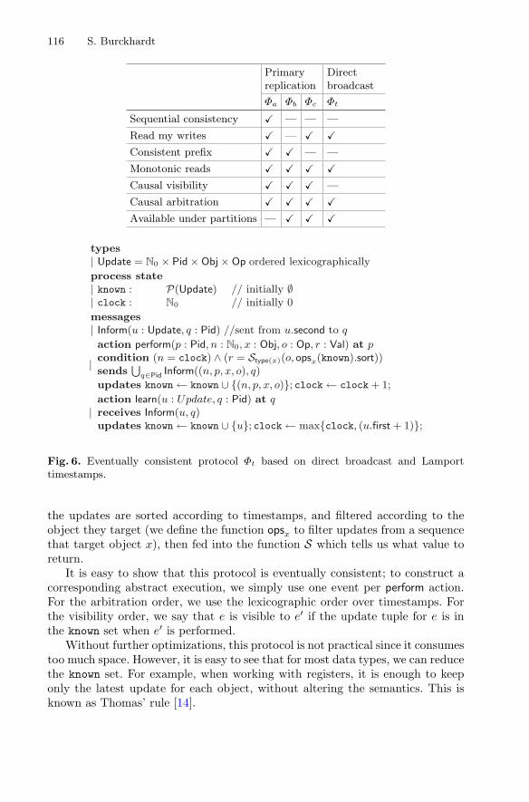
116 S. Burckhardt

Primaryreplication

Directbroadcast

Φa Φb Φc Φt

Sequential consistency � — — —

Read my writes � — � �Consistent prefix � � — —

Monotonic reads � � � �Causal visibility � � � —

Causal arbitration � � � �Available under partitions — � � �

types| Update = N0 × Pid × Obj × Op ordered lexicographically

process state| known : P(Update) // initially ∅| clock : N0 // initially 0

messages| Inform(u : Update, q : Pid) //sent from u.second to q

|action perform(p : Pid, n : N0, x : Obj, o : Op, r : Val) at pcondition (n = clock) ∧ (r = Stype(x)(o, opsx(known).sort))sends

⋃q∈Pid Inform((n, p, x, o), q)

updates known ← known ∪ {(n, p, x, o)}; clock ← clock+ 1;

|action learn(u : Update, q : Pid) at qreceives Inform(u, q)updates known ← known ∪ {u}; clock ← max{clock, (u.first+ 1)};

Fig. 6. Eventually consistent protocol Φt based on direct broadcast and Lamporttimestamps.

the updates are sorted according to timestamps, and filtered according to theobject they target (we define the function opsx to filter updates from a sequencethat target object x), then fed into the function S which tells us what value toreturn.

It is easy to show that this protocol is eventually consistent; to construct acorresponding abstract execution, we simply use one event per perform action.For the arbitration order, we use the lexicographic order over timestamps. Forthe visibility order, we say that e is visible to e′ if the update tuple for e is inthe known set when e′ is performed.

Without further optimizations, this protocol is not practical since it consumestoo much space. However, it is easy to see that for most data types, we can reducethe known set. For example, when working with registers, it is enough to keeponly the latest update for each object, without altering the semantics. This isknown as Thomas’ rule [14].


types| Update = Pidsec × Obj × Op × N0

process state| busy : (⊥ ∪ Update) initially ⊥ (secondary)| localcount : N0 initially 0 (secondary)| confirmed : Update∗ initially ε (secondary)

messages| Update(u : Update) //sent from secondary u.first to primary p| Inform(u : Update, q′ : Pidsec) //sent from primary p to secondary q′

action read(q : Pidsec, x : Obj, o : Op, r : Val) at q (secondary)| condition (busy = ⊥) ∧ (o is a read-only operation)| condition r = Stype(x)(o, opsx(confirmed))

action update(q : Pidsec, x : Obj, o : Op, l : N0) at q (secondary)| condition (busy = ⊥) ∧ (o is a update-only operation) ∧ (l = localcount)| sends Update(q, x, o, l)| updates busy ← (q, x, o, l); localcount ← localcount+ 1;

action perform(u : Update) at p (primary)| receives Update(u)| sends ⋃

q′∈Pid Inform(u, q′)

action learn(u : Update, q′ : Pidsec) at q′ (secondary)| receives in-order Inform(u)| updates confirmed ← confirmed · u| updates if busy = uthenbusy ← ⊥

Fig. 7. Sequentially consistent protocol Φa based on primary replication, supportinglocal reads on secondaries, for some primary process p ∈ Pid and secondary processesPidsec ⊆ Pid.

Sequentially Consistent Protocol Φa. Figure 7 shows a protocol basedon primary replication. Operations are performed at the secondary replicas,with identifiers Pidsec ⊆ Pid. Each secondary replica stores a sequence confirmedof updates it received from the primary replica, using in-order delivery. Read-only operations are performed locally on secondary replicas, by consulting theupdates stored in confirmed. Other operations issued on secondary replicasare broken down into beginoperation and endoperation. beginoperation sends theupdate to the primary. Nothing else can happen on the secondary, until thissame update is confirmed by the primary.

Executions are sequentially consistent. To obtain an abstract execution,define the events to be the actions read and perform, and define → to be thetotal order that we obtain by (1) taking the total order in which the performevents appear in the execution, and (2) inserting read into this chain anywhereafter the last update confirmed before the local read, and before the next updateconfirmed after the local read.

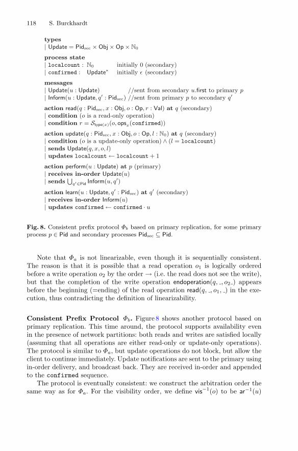
118 S. Burckhardt


process state| localcount : N0 initially 0 (secondary)| confirmed : Update∗ initially ε (secondary)


action read(q : Pidsec, x : Obj, o : Op, r : Val) at q (secondary)| condition (o is a read-only operation)| condition r = Stype(x)(o, opsx(confirmed))

action update(q : Pidsec, x : Obj, o : Op, l : N0) at q (secondary)| condition (o is a update-only operation) ∧ (l = localcount)| sends Update(q, x, o, l)| updates localcount ← localcount+ 1

action perform(u : Update) at p (primary)| receives in-order Update(u)| sends ⋃


action learn(u : Update, q′ : Pidsec) at q′ (secondary)| receives in-order Inform(u)| updates confirmed ← confirmed · u

Fig. 8. Consistent prefix protocol Φb based on primary replication, for some primaryprocess p ∈ Pid and secondary processes Pidsec ⊆ Pid.

Note that Φa is not linearizable, even though it is sequentially consistent.The reason is that it is possible that a read operation o1 is logically orderedbefore a write operation o2 by the order → (i.e. the read does not see the write),but that the completion of the write operation endoperation(q, , o2 ) appearsbefore the beginning (=ending) of the read operation read(q, , o1, ) in the exe-cution, thus contradicting the definition of linearizability.

Consistent Prefix Protocol Φb. Figure 8 shows another protocol based onprimary replication. This time around, the protocol supports availability evenin the presence of network partitions: both reads and writes are satisfied locally(assuming that all operations are either read-only or update-only operations).The protocol is similar to Φa, but update operations do not block, but allow theclient to continue immediately. Update notifications are sent to the primary usingin-order delivery, and broadcast back. They are received in-order and appendedto the confirmed sequence.

The protocol is eventually consistent: we construct the arbitration order thesame way as for Φa. For the visibility order, we define vis−1(o) to be ar−1(u)



process state| localcount : N0 initially 0 (secondary)| pending : Update∗ initially ε (secondary)| confirmed : Update∗ initially ε (secondary)


|action read(q : Pidsec, x : Obj, o : Op, r : Val) at q (secondary)| condition (o is a read-only operation)| condition r = Stype(x)(o, opsx(confirmed) · opsx(pending))

|action update(q : Pidsec, x : Obj, o : Op, l : N0) at q (secondary)| condition (o is a update-only operation) ∧ (l = localcount)| sends Update(q, x, o, l)| updates localcount ← localcount+ 1; pending ← pending · (q, x, u, l)

|action perform(u : Update) at p (primary)| receives in-order Update(u)| sends ⋃


|action learn(u : Update, q′ : Pidsec) at q′ (secondary)| receives in-order Inform(u)| updates confirmed ← confirmed · u; if q = q′ then pending ← pending.remove(u)

Fig. 9. Read-my-writes protocol Φc based on primary replication, for some primaryprocess p ∈ Pid and secondary processes Pidsec ⊆ Pid.

where u is the last operation in confirmed at the time o is performed. Thus, theprotocol satisfies consistent prefix.

Read-My-Writes Protocol Φc. Figure 9 shows yet another protocol based onprimary replication. This time, we want to support read-my-writes, so we locallystore a sequence pending of operations that have been sent to the primary, butnot confirmed yet. When performing reads or writes locally, we use not only theupdates in confirmed, but also append the updates in pending.

References

1. Brewer, E.A.: Towards robust distributed systems (abstract). In: PODC 2000(2000)

2. Burckhardt, S.: Consistency in distributed systems. LASER Summer School SlideDecks (2013). http://sdrv.ms/1dWFsBQ

3. Burckhardt, S.: Principles of eventual consistency. Found. Trends Program. Lang.1(1–2), 1–150 (2014)

4. Burrowsm, M.: The Chubby lock service for loosely-coupled distributed systems.In: Operating Systems Design and Implementation, pp. 335–350 (2006)

http://sdrv.ms/1dWFsBQ

120 S. Burckhardt

5. Cachin, C., Guerraoui, R., Rodrigues, L.: Introduction to Reliable and SecureDistributed Programming, 2nd edn. Springer, Heidelberg (2011)

6. Dill, D.L.: The murphi verification system. In: Computer Aided Verification, pp.390–393 (1996)

7. Fischer, M.J., Lynch, N.A., Paterson, M.S.: Impossibility of distributed consensuswith one faulty process. J. ACM 32, 374–382 (1982)

8. Gilbert, S., Lynch, N.: Brewer’s conjecture and the feasibility of consistent, avail-able, partition-tolerant web services. SIGACT News 33(2), 51–59 (2002)

9. Hunt, P., Konar, M., Junqueira, F.P., Reed, B.: Zookeeper: wait-free coordina-tion for internet-scale systems. In: Proceedings of the 2010 USENIX Conferenceon USENIX Annual Technical Conference, USENIXATC 2010, p. 11. USENIXAssociation, Berkeley (2010)

10. Lamport, L.: Time, clocks, and the ordering of events in a distributed system.Commun. ACM 21(7), 558–565 (1978)

11. Lamport, L.: The part-time parliament. ACM Trans. Comput. Syst. 16, 133–169(1998)

12. Lloyd, W., Freedman, M.J., Kaminsky, M., Andersen, D.G.: Don’t settle foreven-tual: scalable causal consistency for wide-area storage with COPS. In: SOSP 2011(2011)

13. Terry, D.: Replicated Data Consistency Explained Through Baseball (2011)14. Thomas, R.H., Beranek, B.: A majority consensus approach to concurrency control

for multiple copy databases. ACM Trans. Database Syst. 4, 180–209 (1979)

consistency in distributed systems - · pdf fileconsistency in distributed systems sebastian...

Documents