energies

Article

Schedule Optimization in a Smart MicrogridConsidering Demand Response Constraints

Julian Garcia-Guarin 1 , David Alvarez 1 , Arturo Bretas 2 and Sergio Rivera 1,2,*1 Electrical and Electronics Engineering Department, Engineering Faculty, Universidad Nacional de Colombia,

Bogotá 111321, Colombia; pjgarciag@unal.edu.co (J.G.-G.); dlalvareza@unal.edu.co (D.A.)2 Engineering Faculty, University of Florida, Gainesville, FL 32611, USA; arturo@ece.ufl.edu* Correspondence: srriverar@unal.edu.co; Tel.: +57-1-320-463-2806

Received: 23 July 2020; Accepted: 1 September 2020; Published: 3 September 2020�����������������

Abstract: Smart microgrids (SMGs) may face energy rationing due to unavailability of energyresources. Demand response (DR) in SMGs is useful not only in emergencies, since load cuts might beplanned with a reduction in consumption but also in normal operation. SMG energy resources includestorage systems, dispatchable units, and resources with uncertainty, such as residential demand,renewable generation, electric vehicle traffic, and electricity markets. An aggregator can optimize thescheduling of these resources, however, load demand can completely curtail until being neglected toincrease the profits. The DR function (DRF) is developed as a constraint of minimum size to supplythe demand and contributes solving of the 0-1 knapsack problem (KP), which involves a combinatorialoptimization. The 0-1 KP stores limited energy capacity and is successful in disconnecting loads.Both constraints, the 0-1 KP and DRF, are compared in the ranking index, load reduction percentage,and execution time. Both functions turn out to be very similar according to the performance of theseindicators, unlike the ranking index, in which the DRF has better performance. The DRF reduces to25% the minimum demand to avoid non-optimal situations, such as non-supplying the demand andhas potential benefits, such as the elimination of finite combinations and easy implementation.

Keywords: load shedding; optimization of energy demand supply; smart microgrid scheduling;0-1 knapsack problem

1. Introduction

User participation has become of great value in smart grids management. Cooperation amongusers allows decision-making more flexibility, through the use of demand response (DR). Customers canbe included in DR programs either by changing their habits or by implementing load control [1].DR can be analyzed from two approaches: the first considers the power quality that is affected bydisturbances, such as harmonics, inter-harmonics, phase unbalance, phase jump, and temperatureeffects due to overloads [2,3]. The second encompasses demand benefits for reducing operating costs,improving aggregator profits, and mitigating market power [3,4]. This research falls under the secondgroup, which saves energy through demand management [5].

Demand management can consider demand forecasts, load curtailment, and combinatorialoptimization with DR [6,7]. This type of combinatorial optimization problem has several applications forload shedding [8]. Heuristic techniques have been applied to solve this problem with non-deterministicpolynomial times, also called NP-hard problems [8,9]. This type of problem can arise as a subproblemor a constraint [5,8,9]. The solution was presented as a combination of a series of user decisions [5,8,9].In microgrids, load shedding was modeled through the 0-1 knapsack problem (KP), which is classifiedas an NP-hard problem [8]. In using this technique, the possibilities and solution times are exponentiallyincreased with 2N [8]. The 0-1 KP problem was solved with heuristic algorithms and Lagrangian

Energies 2020, 13, 4567; doi:10.3390/en13174567 www.mdpi.com/journal/energies

Energies 2020, 13, 4567 2 of 18

multipliers. For example, Cuckoo Search and Tabu Search are heuristic algorithms that are appliedefficiently by solving multidimensional 0-1 KP [8,10]. In addition, the method of Lagrangian multipliersis implemented with integer programming. Results show that execution time is polynomial and issimilar to other findings [11].

Load restoration has been addressed with 0-1 KP in microgrids. Consumer supply is an importantprocedure after the smart microgrid (SMG) is out of service [12,13]. For example, failures and blackoutscan deteriorate customer satisfaction and restoration of power supply is essential [12,13]. DR programsshare the objectives of ensuring user welfare and supplying essential loads [14]. Energy must besupplied at low cost and supplying critical loads [12,13]. The energy supply is optimized throughheuristic techniques [12,13]. Consequently, DR programs are supported by load restoration programs,in both cases the aim is to ensure the energy supply of a group of users.

Optimization techniques with heuristics have been widely studied [15]. SMGs comprise interactingelements such as residential loads with DR programs, distributed electric vehicles (EVs), energy storagesystems (ESSs), generation with renewable energies, and dispatchable units [13,14]. SMGs may alsobe subject to sources of uncertainty that further complicate operation, such as residential demand,renewable generation, traffic of EVs, and electricity markets [13,15]. For example, a comparativeanalysis is performed between various algorithms for a SMG model [9,16]. The variable neighborhoodsearch-differential evolutionary particle swarm optimization (VNS-DEEPSO) algorithm turned outto be better than the chaotic evolutionary particle swarm optimization (PSO), differential evolution(DE) with stochastic selection, enhanced velocity differential evolutionary PSO, firefly, improvedchaotic DEEPSO, improved DE, PSO with global best perturbation, and unified PSO algorithms [16].Research on these algorithms suggests implementing constraints for DR [17–19].

1.1. Motivation of This Paper

Operational costs optimization with heuristics alleviates renewable energy disadvantages such asintermittency and fluctuations that can be addressed with the management of ESSs. Heuristics withprobabilistic analysis provide robust solutions to the uncertainty of renewables [20]. In addition,the energy supply is considered as an additional objective under criteria of frequency, duration,and magnitude [4,20]. For example, the reduction of operational costs and energy supply are consideredin multi-objective optimization problems, this approach presents as a drawback of multiple optimalsolutions on the Pareto front [4,20]. However, in the traditional approach the problem is addressedconsidering 0-1 KP restrictions, however the polynomial execution times make it difficult to analyzereal microgrids [14]. Solving problems involving polynomial execution times, robust solutions in SMGswith uncertainty, and addressing multiple criteria in a single objective function motivates the findingsof this research.

1.2. Contribution of This Paper

This article presents an implementation of 0-1 KP constraints for DR. In addition, the DR function(DRF) is developed as a contribution of this research that solves the 0-1 KP, which indeed involvescombinatorial optimization. Both techniques, DRF and 0-1 KP, are evaluated in a SMG modelconsidering an aggregator that seeks social welfare and supplies essential loads. The aggregatorschedules resources with or without uncertainty. The uncertainty resources are EVs trips, renewablegeneration, loads with DR, and energy market prices [21]. The resources without uncertainty aredistributed generators (DGs) and ESSs. Additionally, this article makes the following contributions:

(1) The implementation of 0-1 KP in a SMG model. 0-1 KP is formulated in two levels. In the firstlevel the demand is grouped, and in the second level the demand is discretized into hour blocks.The refinement of the blocks depends on the computing capacity. Results are measured in termsof the ranking index (RI), load reduction percentage, and execution time. The RI is calculated asthe sum of the average profits and their standard deviation.

Energies 2020, 13, 4567 3 of 18

(2) DRF is developed to solve the 0-1 KP. DRF is compared with 0-1 KP in terms of the RI, load reductionpercentage, and execution time. The outstanding outcomes of DRF are similar to those of the0-1 KP. However, DRF stands out for the following characteristics. DRF works with continuedvariables, so DRF has no problem of refinement. In addition, DRF needs no additional executiontime for preloading combinations, since the polynomial time in 0-1 KP and its function are easierto implement than 0-1 KP.

The article presents the following structure: Section 2 summarizes the state of the art, Section 3presents the SMG model, Section 4 formulates 0-1 KP and DRF, Section 5 contains the results,and Section 6 presents the main conclusions of the research.

2. State of the Art

Table 1 shows the SMG models with energy resources that are subject to 0–1 KP and DRFrestrictions [18–26]. These models are listed from 1 to 9 and are described in the following. The SMGmodel 1 considers a maximum generation capacity at 0-1 KP and is solved by using binary variables.The SMG model 1 also considers the maximization of the benefits of SMG [14]. The 0-1 KP solutionis successful. However, this model has the problem of polynomial times. Since the SMG model 1represents a simple microgrid, it lacks elements such as load with DR, market prices, EVs, and ESSs.Therefore, the implementation of the SMG model 1 is feasible in didactic and short-range scenarios ofactual SMGs [14].

The SMG model 2 gathers elements such as DGs, photovoltaic (PV) generation, external suppliers,load with DR, market prices, EVs, and ESSs [13,17,27,28]. The SMG model 2 also has sourcesof uncertainty such as residential demand, renewable generation, traffic of EVs, and electricitymarkets [13,17,27]. The model is based on the operation of a residential microgrid [16]. However,the residential customer demand is unattended after the optimization process, that is, the load demandis close to zero. In demand management, this is an unwanted solution [12,16]. The SMG model 2is improved with a battery swapping station for EVs and sets a DRF as a constraint [22]. However,DRF is a target rather than a constraint in [4]. Therefore, the new implementation of the DRF lacksa previous study for the implementation with loads with DR.

Table 1. Review of microgrids energy resources with 0-1 knapsack problem (KP) and demand responsefunction (DRF).

No. Gen ESS DR EVs 0-1 KP DRF Uncertainty Sources

1 Yes No Yes No Yes No Not reported [14]2 Yes Yes Yes Yes No Yes EVs, renewable resources, electricity markets, and loads with DR [22]3 No No Yes No No No Electricity markets and loads with DR [23]4 Yes Yes No No No No Renewable resources and loads [24]5 Yes Yes Yes No No No Renewable resources, loads, and market prices [25]6 Yes Yes No Yes No No Renewable resources, loads, and EVs [26]7 Yes Yes Yes No No No Renewable resources, loads, and market prices [27]8 Yes Yes No No No No Not reported [29]9 Yes No No No No No Not reported [30,31]

10 Yes Yes Yes Yes Yes Yes EVs, renewable resources, electricity markets, and loads with DR(this model is implemented in this research)

The residential power system model 3 aims to improve the economic benefits [23]. This modelconsiders the use of smart meters in SMGs [1] as well as load uncertainty and price volatility in realtime [23]. This model has no restrictions in optimization, which ensures a good state of the demand,such as 0-1 KP and DRF [23]. The analysis does not consider EVs and ESSs [23]. The power systemmodel 4 takes into account the predictive forecast but not load shedding [24]. In addition, batteriesand generation with combined heat and power and renewable are considered to increase profits [24].This model includes neither DR programs nor EVs [24].

The model 5 of distributed resources supplies the demand side with renewable energy [25] andaims to reduce CO2 emissions and energy costs. The technique restricts the energy demand supplying

Energies 2020, 13, 4567 4 of 18

and is similar to 0-1 KP, but in this case seven probability scenarios are studied. These seven scenariosare obtained by using a scenario reduction technique. This model is strictly limited to plausiblescenarios in uncertain environments; therefore, it can find plausible but not optimal solutions [25].

The smart grid model 6 comprises EVs, ESSs, and renewable generation. This model aims toreduce operating costs and lower CO2 emissions from thermal power plants [26]. This model predictsthe load; however, it warns of deviations from the actual load. The model includes no implementationof load with DR [26]. The small-scale model 7 of smart grid aims to maximize the profits in the gridand considers a system with DGs, renewable energies, and ESSs [27]. In this model, the loads arerepresented by an agent that controls the electric power and exchanges information with other agentsin the network [27]. The major drawback of this formulation is that the model lacks load demandmanagement strategies and is difficult to reproduce. Nevertheless, it provides viable results despitehaving no load restrictions.

The microgrid model 8 reduces operation costs while the dispatchable generation units and thestorage of energy are scheduled. Errors for forecasting demand in the operation are recommended tobe studied in future works. The microgrid model 8 highlights operations to optimize costs, such asload curtailment and load shifting [29]. Power network models in 9 analyze generation costs, powerlosses, emissions, and validate an evolutionary hybrid algorithm. This research has demonstrated theinterest of the scientific community in validating optimization algorithms with multiple tests. However,the study neglects sources of uncertainty, ESSs, VEs, loads with response to demand, and penaltiesfor not supplying the demand [32]. Table 2 summarizes the limitations presented in the review ofthis section.

The SMG model 10 is implemented in this research and overcomes some drawbacks describedin previous literature. First, this model addresses residential loads with DR programs, EVs, ESSs, DGs,and renewable resources. An aggregator aims to increase profits and can negotiate the buy/sell energyin electricity markets. The microgrid considers uncertainty conditions that are more challenging in theoperation, such as renewable generation forecasts, trip planning with EVs, market price volatility,and load forecast.

Table 2. Limitations of the review of microgrids with 0-1 KP and DRF.

No. Limitations of the Review of Microgrids Energy Resources with 0-1 KP and DRF.

1 The model 1 lacks elements such as load with DR, market prices, EVs, and ESSs [14].

2 The residential customer demand is unattended after the optimization process. In demand management, this is anunwanted solution [22].

3 The model 3 has no restrictions in optimization, which ensures a good state of the demand, such as 0-1 KP and DRF [23].4 The model 4 does not include either DR programs or EVs [24].

5 The model 5 is strictly limited to plausible scenarios in uncertain environments; therefore, it can find feasible but notoptimal solutions [25].

6 The model 6 includes no implementation of load with DR [26].

7 The major drawback of this formulation is that the model 7 lacks load demand management strategies and is difficult toreproduce [27].

8 Errors for forecasting demand in the operation are recommended to be studied in future works [29].9 The study neglects sources of uncertainty, ESSs, VEs, loads with DR, and penalties for not supplying the demand [31].

10 Model 10 overcomes the above limitations.

The SMG model 10 overcomes the weaknesses mentioned in previous models, such as ensuringthat the demand is met, integrating DR programs, generating a feasible SMG model for optimization,and creating a reproducible method. This model includes 0-1 KP and DRF to optimize the loads withDR. The 0-1 KP implementation consists of discretizing the load for its optimization and guaranteeingthat the demand is satisfied. DRF is a constraint in the objective function to ensure welfare of thedemand. This model is the most complete according to the literature review shown in Table 1 thatincludes sources of uncertainty, elements of the SMG, and 0-1 KP and DRF demand restrictions.

Various heuristic algorithms have been studied to solve SMG models. The resulting VNS-DEEPSOalgorithm has the highest performance of the algorithms mentioned above according to [12,16].The mechanisms implemented in this heuristic are described below.

Energies 2020, 13, 4567 5 of 18

2.1. VNS-DEEPSO Algorithm

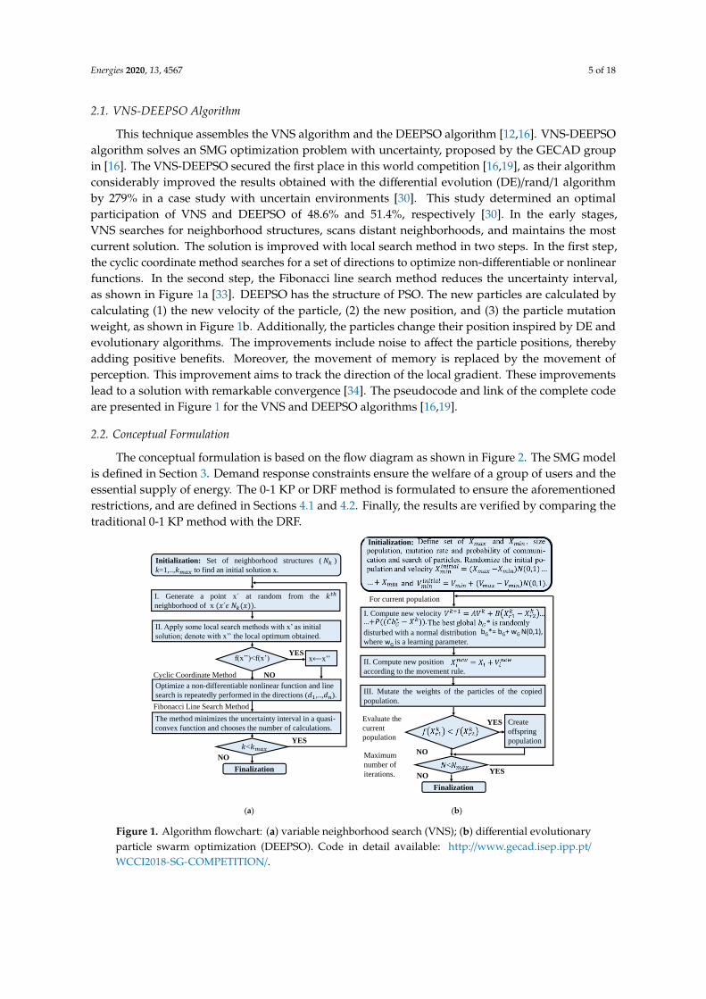
This technique assembles the VNS algorithm and the DEEPSO algorithm [12,16]. VNS-DEEPSOalgorithm solves an SMG optimization problem with uncertainty, proposed by the GECAD groupin [16]. The VNS-DEEPSO secured the first place in this world competition [16,19], as their algorithmconsiderably improved the results obtained with the differential evolution (DE)/rand/1 algorithmby 279% in a case study with uncertain environments [30]. This study determined an optimalparticipation of VNS and DEEPSO of 48.6% and 51.4%, respectively [30]. In the early stages,VNS searches for neighborhood structures, scans distant neighborhoods, and maintains the mostcurrent solution. The solution is improved with local search method in two steps. In the first step,the cyclic coordinate method searches for a set of directions to optimize non-differentiable or nonlinearfunctions. In the second step, the Fibonacci line search method reduces the uncertainty interval,as shown in Figure 1a [33]. DEEPSO has the structure of PSO. The new particles are calculated bycalculating (1) the new velocity of the particle, (2) the new position, and (3) the particle mutationweight, as shown in Figure 1b. Additionally, the particles change their position inspired by DE andevolutionary algorithms. The improvements include noise to affect the particle positions, therebyadding positive benefits. Moreover, the movement of memory is replaced by the movement ofperception. This improvement aims to track the direction of the local gradient. These improvementslead to a solution with remarkable convergence [34]. The pseudocode and link of the complete codeare presented in Figure 1 for the VNS and DEEPSO algorithms [16,19].

2.2. Conceptual Formulation

The conceptual formulation is based on the flow diagram as shown in Figure 2. The SMG modelis defined in Section 3. Demand response constraints ensure the welfare of a group of users and theessential supply of energy. The 0-1 KP or DRF method is formulated to ensure the aforementionedrestrictions, and are defined in Sections 4.1 and 4.2. Finally, the results are verified by comparing thetraditional 0-1 KP method with the DRF.

Energies 2020, 13, x FOR PEER REVIEW 6 of 19

(a) (b)

Figure 1. Algorithm flowchart: (a) variable neighborhood search (VNS); (b) differential evolutionary

particle swarm optimization (DEEPSO). Code in detail available:

http://www.gecad.isep.ipp.pt/WCCI2018-SG-COMPETITION/.

Figure 2. Conceptual formulation of a smart microgrid (SMG) with DR constraints.

3. Smart Microgrid Model

The aggregator aims to improve the SMG profits in the day-ahead operation (𝐷𝑎𝑦 + 1) [30]. Day-

ahead scheduling of residential microgrid is considered an optimization problem [21]; this microgrid

located in Portugal includes EVs, residential loads, and an energy storage system, as shown in Figure

3 [35]. A SMG scheduling problem contains 17 aggregated PV generators (17 agg.) in a group of PV

generation [36]. This SMG model contains different types of variables, such as binary, continuous,

and discrete, by using mixed integer programming [16,21]. The aggregator reduces the operational

costs (OCs) and maximizes the incomes (In), as shown in Equation (1) [21].

Initialization: Set of neighborhood structures ( )

k=1,.., to find an initial solution x.

I. Generate a point x at random from the

neighborhood of x .

II. Apply some local search methods with x’ as initial

solution; denote with x’’ the local optimum obtained.

f(x’’)<f(x’) x⟵x’’YES

Optimize a non-differentiable nonlinear function and line

search is repeatedly performed in the directions ( ,.., ).

Cyclic Coordinate Method NO

The method minimizes the uncertainty interval in a quasi-

convex function and chooses the number of calculations.

Fibonacci Line Search Method

<YES

NO

Finalization

I. Compute new velocity

For current population

disturbed with a normal distribution

where wG is a learning parameter.

bG*= bG+ wG N(0,1),

II. Compute new position

according to the movement rule.

III. Mutate the weights of the particles of the copied

population.

Evaluate the

current

population

YES

NO

Create

offspring

population

YESNO

Finalization

Maximum

number of

iterations.

Initialization:

Equation (14)

Fitness Constraintfunction of demand

response

3. Fitness function of smart microgrid model

Loads with demand response

4.1 0-1 knapsack problem 4.2. Constraints of demand response

Optimization with the algorithm VNS-DEEPSO

4.1.1 Demand grouping

4.1.2 Demand discretization

5. Verification of results

Contributions of this research

Figure 1. Algorithm flowchart: (a) variable neighborhood search (VNS); (b) differential evolutionaryparticle swarm optimization (DEEPSO). Code in detail available: http://www.gecad.isep.ipp.pt/WCCI2018-SG-COMPETITION/.

Energies 2020, 13, 4567 6 of 18

Energies 2020, 13, x FOR PEER REVIEW 6 of 19

(a) (b)

Figure 1. Algorithm flowchart: (a) variable neighborhood search (VNS); (b) differential evolutionary

particle swarm optimization (DEEPSO). Code in detail available:

http://www.gecad.isep.ipp.pt/WCCI2018-SG-COMPETITION/.

Figure 2. Conceptual formulation of a smart microgrid (SMG) with DR constraints.

3. Smart Microgrid Model

The aggregator aims to improve the SMG profits in the day-ahead operation (𝐷𝑎𝑦 + 1) [30]. Day-

ahead scheduling of residential microgrid is considered an optimization problem [21]; this microgrid

located in Portugal includes EVs, residential loads, and an energy storage system, as shown in Figure

3 [35]. A SMG scheduling problem contains 17 aggregated PV generators (17 agg.) in a group of PV

generation [36]. This SMG model contains different types of variables, such as binary, continuous,

and discrete, by using mixed integer programming [16,21]. The aggregator reduces the operational

costs (OCs) and maximizes the incomes (In), as shown in Equation (1) [21].

Initialization: Set of neighborhood structures ( )

k=1,.., to find an initial solution x.

I. Generate a point x at random from the

neighborhood of x .

II. Apply some local search methods with x’ as initial

solution; denote with x’’ the local optimum obtained.

f(x’’)<f(x’) x⟵x’’YES

Optimize a non-differentiable nonlinear function and line

search is repeatedly performed in the directions ( ,.., ).

Cyclic Coordinate Method NO

The method minimizes the uncertainty interval in a quasi-

convex function and chooses the number of calculations.

Fibonacci Line Search Method

<YES

NO

Finalization

I. Compute new velocity

For current population

disturbed with a normal distribution

where wG is a learning parameter.

bG*= bG+ wG N(0,1),

II. Compute new position

according to the movement rule.

III. Mutate the weights of the particles of the copied

population.

Evaluate the

current

population

YES

NO

Create

offspring

population

YESNO

Finalization

Maximum

number of

iterations.

Initialization:

Equation (14)

Fitness Constraintfunction of demand

response

3. Fitness function of smart microgrid model

Loads with demand response

4.1 0-1 knapsack problem 4.2. Constraints of demand response

Optimization with the algorithm VNS-DEEPSO

4.1.1 Demand grouping

4.1.2 Demand discretization

5. Verification of results

Contributions of this research

Figure 2. Conceptual formulation of a smart microgrid (SMG) with DR constraints.

3. Smart Microgrid Model

The aggregator aims to improve the SMG profits in the day-ahead operation (Day + 1) [30].Day-ahead scheduling of residential microgrid is considered an optimization problem [21];this microgrid located in Portugal includes EVs, residential loads, and an energy storage system,as shown in Figure 3 [35]. A SMG scheduling problem contains 17 aggregated PV generators (17 agg.)in a group of PV generation [36]. This SMG model contains different types of variables, such as binary,continuous, and discrete, by using mixed integer programming [16,21]. The aggregator reduces theoperational costs (OCs) and maximizes the incomes (In), as shown in Equation (1) [21].

Minimize Z = OCDay+1Total − InDay+1

Total (1)Energies 2020, 13, x FOR PEER REVIEW 7 of 19

Figure 3. Residential 25-bus SMG in a 400 V system [35].

𝑀𝑖𝑛𝑖𝑚𝑖𝑧𝑒 𝑍 = 𝑂𝐶𝑇𝑜𝑡𝑎𝑙𝐷𝑎𝑦+1

− 𝐼𝑛𝑇𝑜𝑡𝑎𝑙𝐷𝑎𝑦+1 (1)

The OCs are associated to DGs, ESSs, external supplier (𝑒𝑥𝑡), EVs, PV generation, negative

(𝑖𝑚𝑏−) and positive (𝑖𝑚𝑏+) imbalance by exceeding the generation and shortage of energy, and

curtailable loads with residential DR (𝑐𝑢𝑟𝑡) , as shown in Equation (2) [13,17]. The OCs have a

scenarios distribution probability π (s) and predict the forecast error through Monte Carlo

simulations [21]. These simulations are based on historical data [16]. The scenarios are reduced with

the Soares technique, which is based on statistical metrics. Scenarios are reduced from 5000 to 100

feasible for PV generation, load, and market prices [37]. An EVs simulation tool is employed to

generate the travel route forecast [38]. Table 3 shows the specifications of the microgrid.

Table 3. Specifications of SMG [16].

SMG Energy Resources Capacity (kW) Prices (m.u./kW) Units

DGs 10–100 0.07–0.11 5

External supplier 0–150 0.074–0.16 1

Charge/discharge of ESSs 0–16.6 0.03 2

Charge/discharge of EVs 0–111 0.06 34

Loads with DR 4.06–8.95 0.0375 90

Wholesale/local market 0–100/10 0.021–0.039 1

Forecast (kW)

PV generation 0–106.81 - 1 (17 agg.)

Load 35.82–83.39 - 90

𝑂𝐶𝑇𝑜𝑡𝑎𝑙𝐷𝑎𝑦+1

=

∑∑𝑃𝐷𝐺(𝑖,𝑡) ∙ 𝐶𝐷𝐺(𝑖,𝑡)

𝑁𝐷𝐺

𝑖=1

𝑇

𝑡=1

+∑∑𝑃𝑒𝑥𝑡(𝑖,𝑡) ∙ 𝐶𝑒𝑥𝑡(𝑖,𝑡)

𝑁𝑘

𝑘=1

𝑇

𝑡=1

+⋯

∑∑

(

∑ 𝑃𝑃𝑉(𝑗,𝑡,𝑠) ∙ 𝐶𝑃𝑉(𝑗,𝑡,𝑠)

𝑁𝑃𝑉−𝐷𝐺

𝑗=1

+∑𝑃𝐸𝑆𝑆−(𝑒,𝑡,𝑠) ∙ 𝐶𝐸𝑆𝑆−(𝑒,𝑡,𝑠)

𝑁𝑒

𝑒=1

…

…+∑𝑃𝐸𝑉−(𝑣,𝑡,𝑠) ∙ 𝐶𝐸𝑉−(𝑣,𝑡)

𝑁𝑣

𝑣=1

+∑𝑃𝑐𝑢𝑟𝑡(𝑙,𝑡,𝑠) ∙ 𝐶𝑐𝑢𝑟𝑡(𝑙,𝑡,𝑠)

𝑁𝐿

𝑙=1

…

∑𝑃𝑖𝑚𝑏−(𝑚,𝑡,𝑠) ∙ 𝐶𝑖𝑚𝑏− (𝑚,𝑡,𝑠)

𝑁𝐿

𝑙=1

+∑𝑃𝑖𝑚𝑏+(𝑚,𝑡,𝑠) ∙ 𝐶𝑖𝑚𝑏+ (𝑚,𝑡,𝑠)

𝑁𝐷𝐺

𝑖=1 )

𝑇

𝑡=1

𝑁𝑠

𝑠=1

∙ 𝜋(𝑠)

(2)

The aggregator increases the incomes by selling and buying energy in the wholesale and local

markets, as shown in Equation (3).

Bus 1 MV Network 1Bus 2

Bus 10

Load 3

Bus 3

Load 4

Load 5

Load 6

Load 7

Load 8

Load 10

Load 9

Bus 4

Loads 74-82

Loads 65-73

Loads 47-65

Loads 56-64

Bus 9

Bus 8

Bus 24

Bus 25

Bus 23

Bus 22

Loads 29-37

Loads 38-46

Loads 20-28

Loads 11-19

Bus 7

Bus 6

Bus 20

Bus 21

Bus 18

Bus 19

Loads 1-2

Bus 5

Bus 11

Bus 12

Bus 13

Bus 14

Bus 15

Bus 16

Bus 17

Residential loads; Electric vehicles; Energy storage systems; Photovoltaic generation

3

2

4

2 5

4

3

3

Figure 3. Residential 25-bus SMG in a 400 V system [35].

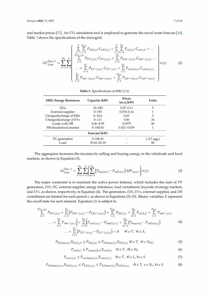
The OCs are associated to DGs, ESSs, external supplier (ext), EVs, PV generation, negative (imb−)and positive (imb+) imbalance by exceeding the generation and shortage of energy, and curtailableloads with residential DR (curt), as shown in Equation (2) [13,17]. The OCs have a scenarios distributionprobability π (s) and predict the forecast error through Monte Carlo simulations [21]. These simulationsare based on historical data [16]. The scenarios are reduced with the Soares technique, which isbased on statistical metrics. Scenarios are reduced from 5000 to 100 feasible for PV generation, load,

Energies 2020, 13, 4567 7 of 18

and market prices [37]. An EVs simulation tool is employed to generate the travel route forecast [38].Table 3 shows the specifications of the microgrid.

OCDay+1Total =

NS∑s=1

T∑t=1

T∑t=1

NDG∑i=1

PDG(i,t)·CDG(i,t) +T∑

t=1

Nk∑k=1

Pext(i,t)·Cext(i,t) + . . .

NPV−DG∑j=1

PPV( j,t,s)·CPV( j,t,s) +Ne∑

e=1PESS−(e,t,s)·CESS−(e,t,s) . . .

. . .+Nv∑

v=1PEV−(v,t,s)·CEV−(v,t) +

NL∑l=1

Pcurt(l,t,s)·Ccurt(l,t,s)...

NL∑l=1

Pimb−(m,t,s)·Cimb−(m,t,s) +NDG∑i=1

Pimb+(m,t,s)·Cimb+(m,t,s)

·π(s) (2)

Table 3. Specifications of SMG [16].

SMG Energy Resources Capacity (kW) Prices(m.u./kW) Units

DGs 10–100 0.07–0.11 5External supplier 0–150 0.074–0.16 1

Charge/discharge of ESSs 0–16.6 0.03 2Charge/discharge of EVs 0–111 0.06 34

Loads with DR 4.06–8.95 0.0375 90Wholesale/local market 0–100/10 0.021–0.039 1

Forecast (kW)

PV generation 0–106.81 - 1 (17 agg.)Load 35.82–83.39 - 90

The aggregator increases the incomes by selling and buying energy in the wholesale and localmarkets, as shown in Equation (3).

InDay+1Total =

NS∑s′=1

T∑t=1

Nm∑m=1

(Pbuy(m,t) − Psell(m,t)

)·MP(m,t,s)

·π(s) (3)

The major constraint is to maintain the active power balance, which includes the sum of PVgeneration, ESS, DG, external supplier, energy imbalance, load curtailment, buy/sale of energy markets,and EVs, as shown, respectively, in Equation (4). The generation, ESS, EVs, external supplier, and DRcurtailment are limited for each period t, as shown in Equations (5)–(9). Binary variables X representthe on/off state for each element. Equation (1) is subject to:

NPV−DG∑j=1

PPV( j,t,s) +Ne∑

e=1

(PESS−(e,t,s) − PESS+(e,t,s)

)+

NDG∑i=1

PDG(i,s) +NK∑k=1

Pext(k,t) +NDG∑i=1

Pimb+(i,t,s)

. . .+NL∑l=1

Pimb−(l,t,s)

)+

NL∑l=1

(Pcurt(l,t,s) − Pload(l,t,s)) +

Nm∑m=1

(Pbuy(m,t) − Psell(m,t,s)

). . .+

Nv∑v=1

(PEV−(v,t,s) − PEV+(v,t,s)

)= 0 ∀t ε T, ∀s ε S,

(4)

PDGmin(i,t)XDG(i,t) ≤ PDG(i,t) ≤ PDGmax(i,t)XDG(i,t) ∀t ε T, ∀i ε NDG (5)

Pext(k,t) ≤ Pextmax(k,t)Xext(k,t) ∀t ε T, ∀k ε Nk (6)

Pcur(l,t,s) ≤ Pcurtmax(l,t,s)Xcurt(l,t,s) ∀t ε T, ∀l ε L,∀s ε S (7)

PESSmin(e,t,s)XESS(e,t,s) ≤ PESS(e,t,s) ≤ PESSmax(i,t)XESS(e,t,s) ∀t ε T, e ε Ne,∀s ε S (8)

Energies 2020, 13, 4567 8 of 18

PEVmin(v,t,s)XEV(v,t,s) ≤ PEV(v,t,s) ≤ PEVmax(v,t,s)XEV(v,t,s) ∀t ε T,∀v ε Nv,∀s ε S (9)

e, i, v , k, l ε Z ∀e ε Ne, ∀i ε NDG,∀v ε Nv, ∀k ε Nk,∀l ε L

The maximum number of evaluations of the objective function in Equation (1) is limited to 50,000,as shown in Equation (10). This is calculated by multiplying the number of populations, scenarios,and iterations in Equation (10) [16].

NFEs = NP ∗Ns ∗Niteration. (10)

The RI is calculated with the average of the sum of the mean and the standard deviation dividedinto the number of runs (Nruns) of the objective function [13].

RI =1

Nruns

Nruns∑i=1

(µ(Z) + σ(Z)) (11)

4. Formulation of the 0-1 KP and the DRF

Sections 4.1 and 4.2 present the formulation of 0-1 KP and DRF. Table 4 summarizes theimplementation of the 0-1 KP and DRF formulations that can be carried out using the simulationgeneral framework in the Matlab R2019b program. The minimum demand is scheduled either usingthe step 2a or 2b of Table 4.

Table 4. Simulation general framework.

No. Step Source

1 Download the case study VNS-DEEPSO Data 1 [19]2a Replace 0-1 KP demand groups in search space limits Section 4.12b Add DRF in fitness function of VNS2.m and DEEPSO_RE.m Section 4.2

3 Analysis of results using Send2Organizer.mat, benchmark_Fitness.txt,benchmark_Summary.txt, and benchmark_Time.txt Section 3

1 http://www.gecad.isep.ipp.pt/WCCI2018-SG-COMPETITION/ data from GECAD group.

4.1. Formulation of 0-1 Knapsack Problem 0-1 KP

SMGs are vulnerable to energy shortages; therefore, it is essential to address the problem of poweroutages to increase their reliability. 0-1 KP is widely used to solve this problem based on combinatorialoptimization. The loads of customer are discretized [3]. 0-1 KP is represented by the evaluation ofan objective function that is subject to a constraint. Equation (1) is subject to Equation (12).

Ns∑s=1

T∑t=1

NL∑l=1

Pcurt(l,t,s)·Ccurt(l,t,s)·yn·π(s) ≥

max(

Ns∑s=1

T∑t=1

NL∑l=1

Pcurt(l,t,s)·Ccurt(l,t,s)·π(s)

4

) (12)

∀t ∈ T, ∀l ∈ L, ∀s ∈ S yn ∈ {0, 1} (n ∈ {1, 2, . . . , N})

The problem in Equation (1) is extended by adding a constraint called 0-1 KP. The same analogy fora knapsack applies to Equation (12). The knapsack has a fixed capacity to carry products. The capacityof the knapsack is 25% of the maximum demand which is fixed at the convenience of the microgrid,and the products that fill the knapsack are stochastic scenarios, time periods, and loads. In otherwords, a good state of the demand is ensured, given that the reduction of the demand varies from 25%to 100% of the maximum demand. The off and on state is represented by the variable yn as 0 and 1.The number of discrete variables is represented by N. The problem is addressed in two stages for better

Energies 2020, 13, 4567 9 of 18

compression and is explained in the following subsections. First, the demand is grouped according tosimilar patterns and, second, the demand is disaggregated into discrete variables.

4.1.1. Demand Grouping

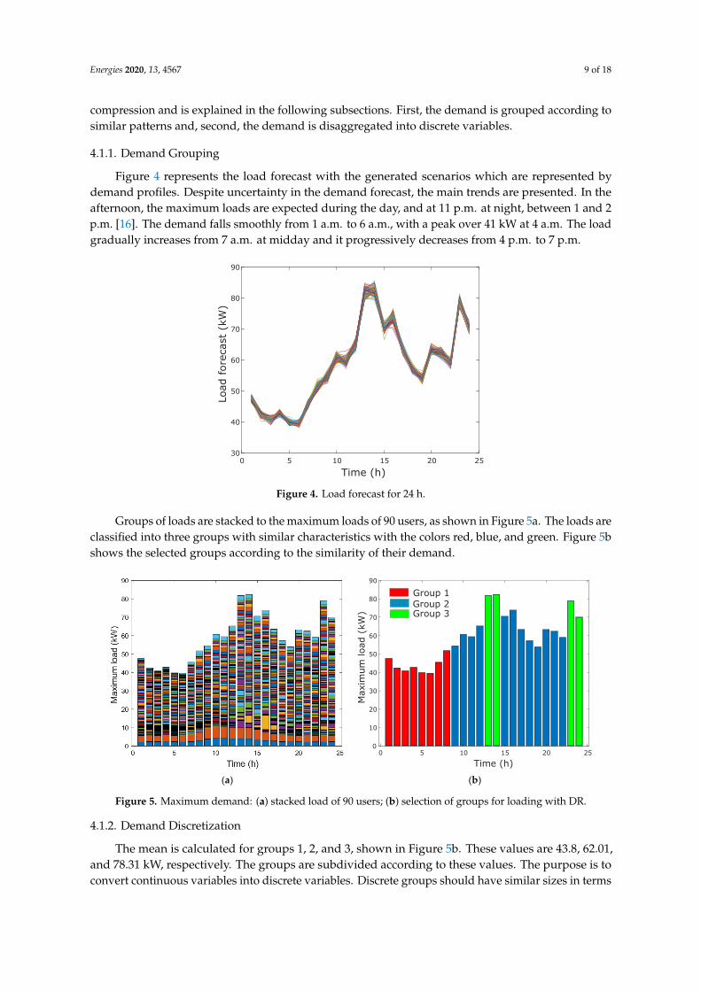
Figure 4 represents the load forecast with the generated scenarios which are represented bydemand profiles. Despite uncertainty in the demand forecast, the main trends are presented. In theafternoon, the maximum loads are expected during the day, and at 11 p.m. at night, between 1 and 2p.m. [16]. The demand falls smoothly from 1 a.m. to 6 a.m., with a peak over 41 kW at 4 a.m. The loadgradually increases from 7 a.m. at midday and it progressively decreases from 4 p.m. to 7 p.m.

Energies 2020, 13, x FOR PEER REVIEW 9 of 19

3 Analysis of results using Send2Organizer.mat, benchmark_Fitness.txt,

benchmark_Summary.txt, and benchmark_Time.txt Section 3

1 http://www.gecad.isep.ipp.pt/WCCI2018-SG-COMPETITION/ data from GECAD group.

4.1. Formulation of 0-1 Knapsack Problem 0-1 KP

SMGs are vulnerable to energy shortages; therefore, it is essential to address the problem of

power outages to increase their reliability. 0-1 KP is widely used to solve this problem based on

combinatorial optimization. The loads of customer are discretized [3]. 0-1 KP is represented by the

evaluation of an objective function that is subject to a constraint. Equation (1) is subject to Equation

(12).

∑∑∑𝑃𝑐𝑢𝑟𝑡(𝑙,𝑡,𝑠) ∙ 𝐶𝑐𝑢𝑟𝑡(𝑙,𝑡,𝑠)

𝑁𝐿

𝑙=1

𝑇

𝑡=1

𝑁𝑠

𝑠=1

∙ 𝑦𝑛 ∙ 𝜋(𝑠)

≥ 𝑚𝑎𝑥 (∑∑∑𝑃𝑐𝑢𝑟𝑡(𝑙,𝑡,𝑠) ∙ 𝐶𝑐𝑢𝑟𝑡(𝑙,𝑡,𝑠)

𝑁𝐿

𝑙=1

𝑇

𝑡=1

𝑁𝑠

𝑠=1

∙𝜋(𝑠)

4)

(12)

∀𝑡 ∈ 𝑇, ∀𝑙 ∈ 𝐿, ∀𝑠 ∈ 𝑆 𝑦𝑛 ∈ {0,1} (𝑛 ∈ {1,2, … , 𝑁})

The problem in Equation (1) is extended by adding a constraint called 0-1 KP. The same analogy

for a knapsack applies to Equation (12). The knapsack has a fixed capacity to carry products. The

capacity of the knapsack is 25% of the maximum demand which is fixed at the convenience of the

microgrid, and the products that fill the knapsack are stochastic scenarios, time periods, and loads.

In other words, a good state of the demand is ensured, given that the reduction of the demand varies

from 25% to 100% of the maximum demand. The off and on state is represented by the variable 𝑦𝑛

as 0 and 1. The number of discrete variables is represented by N. The problem is addressed in two

stages for better compression and is explained in the following subsections. First, the demand is

grouped according to similar patterns and, second, the demand is disaggregated into discrete

variables.

4.1.1. Demand Grouping

Figure 4 represents the load forecast with the generated scenarios which are represented by

demand profiles. Despite uncertainty in the demand forecast, the main trends are presented. In the

afternoon, the maximum loads are expected during the day, and at 11 p.m. at night, between 1 and 2

p.m. [16]. The demand falls smoothly from 1 a.m. to 6 a.m., with a peak over 41 kW at 4 a.m. The load

gradually increases from 7 a.m. at midday and it progressively decreases from 4 p.m. to 7 p.m.

Figure 4. Load forecast for 24 h. Figure 4. Load forecast for 24 h.

Groups of loads are stacked to the maximum loads of 90 users, as shown in Figure 5a. The loads areclassified into three groups with similar characteristics with the colors red, blue, and green. Figure 5bshows the selected groups according to the similarity of their demand.

Energies 2020, 13, x FOR PEER REVIEW 10 of 19

Groups of loads are stacked to the maximum loads of 90 users, as shown in Figure 5a. The loads

are classified into three groups with similar characteristics with the colors red, blue, and green. Figure

5b shows the selected groups according to the similarity of their demand.

(a) (b)

Figure 5. Maximum demand: (a) stacked load of 90 users; (b) selection of groups for loading with DR.

4.1.2. Demand Discretization

The mean is calculated for groups 1, 2, and 3, shown in Figure 5b. These values are 43.8, 62.01,

and 78.31 kW, respectively. The groups are subdivided according to these values. The purpose is to

convert continuous variables into discrete variables. Discrete groups should have similar sizes in

terms of means. Under this condition, groups 1, 2, and 3 are subdivided into 2, 3, and 4, respectively.

Then, 68 discrete variables are obtained for a 24-h period, as shown in Figure 6.

Figure 6. Load forecast for 24 h in the SMG.

In the next step, the number of combinations is calculated for a load of 25% which is selected for

demand convenience. The calculation is represented with 𝑁𝑑 = 68 and 𝑛𝑑 = 17, using Equation (13).

The variables comprise an array of binary variables of 68 × 409.29 quintillion. In the Matlab R2019b

program, the maximum variable size is exceeded, so it does not work with this matrix size. The

computer processor is Core i5-7200—12 GB RAM. The next combination is generated by taking 𝑁𝑑 =

34 and 𝑛𝑑 = 9 with a matrix around 34 × 1715 million variables and by using Equation (13). The

maximum variable size is exceeded again. The next combination is 𝑁𝑑 = 17 and 𝑛𝑑 = 5 that results

in 17 × 127,858. With this matrix size, optimization is feasible.

∑(𝑁𝑑!

(𝑁𝑑 − 𝑛𝑑))

𝑁𝑑

𝑛𝑑

= 𝑁𝐶 (13)

The 24-h period is discretized into 17 loads, as shown in Figure 7. One of the concerns of this

problem is polynomial nondeterministic time, better known as the N-P hard problem. The

polynomial increase is evident [8]. The initial formulation with 68 discrete charges requires a matrix

of the order of quintillion. The half of the discrete loads (34) requires a matrix of millions of discrete

variables. The half of the discrete loads (17) requires an array of thousands of discrete variables. In

other words, the main concern in this type of combinatorial problem is the polynomial calculation

time. In 0-1 KP, additional computation times are avoided by preloading a binary matrix of 17 ×

Hours

Loading block 1 2 3 4 5 6 7 8 9 10 11 12 13 14 15 16 17 18 19 20 21 22 23 24 25 26 27 28 29 30 31 32 33 34 35 36

9 101 2 3 4 5 6 7 8 13 1411 12

Hours

Loading block 37 38 39 40 41 42 43 44 45 46 47 48 49 50 51 52 53 54 55 56 57 58 59 60 58 59 60 58 59 60 61 62 63 64 65 66 67 68

18 19 2015 16 17 18 17 21 22 23 24

Figure 5. Maximum demand: (a) stacked load of 90 users; (b) selection of groups for loading with DR.

4.1.2. Demand Discretization

The mean is calculated for groups 1, 2, and 3, shown in Figure 5b. These values are 43.8, 62.01,and 78.31 kW, respectively. The groups are subdivided according to these values. The purpose is toconvert continuous variables into discrete variables. Discrete groups should have similar sizes in terms

Energies 2020, 13, 4567 10 of 18

of means. Under this condition, groups 1, 2, and 3 are subdivided into 2, 3, and 4, respectively. Then,68 discrete variables are obtained for a 24-h period, as shown in Figure 6.

Energies 2020, 13, x FOR PEER REVIEW 10 of 19

Groups of loads are stacked to the maximum loads of 90 users, as shown in Figure 5a. The loads

are classified into three groups with similar characteristics with the colors red, blue, and green. Figure

5b shows the selected groups according to the similarity of their demand.

(a) (b)

Figure 5. Maximum demand: (a) stacked load of 90 users; (b) selection of groups for loading with DR.

4.1.2. Demand Discretization

The mean is calculated for groups 1, 2, and 3, shown in Figure 5b. These values are 43.8, 62.01,

and 78.31 kW, respectively. The groups are subdivided according to these values. The purpose is to

convert continuous variables into discrete variables. Discrete groups should have similar sizes in

terms of means. Under this condition, groups 1, 2, and 3 are subdivided into 2, 3, and 4, respectively.

Then, 68 discrete variables are obtained for a 24-h period, as shown in Figure 6.

Figure 6. Load forecast for 24 h in the SMG.

In the next step, the number of combinations is calculated for a load of 25% which is selected for

demand convenience. The calculation is represented with 𝑁𝑑 = 68 and 𝑛𝑑 = 17, using Equation (13).

The variables comprise an array of binary variables of 68 × 409.29 quintillion. In the Matlab R2019b

program, the maximum variable size is exceeded, so it does not work with this matrix size. The

computer processor is Core i5-7200—12 GB RAM. The next combination is generated by taking 𝑁𝑑 =

34 and 𝑛𝑑 = 9 with a matrix around 34 × 1715 million variables and by using Equation (13). The

maximum variable size is exceeded again. The next combination is 𝑁𝑑 = 17 and 𝑛𝑑 = 5 that results

in 17 × 127,858. With this matrix size, optimization is feasible.

∑(𝑁𝑑!

(𝑁𝑑 − 𝑛𝑑))

𝑁𝑑

𝑛𝑑

= 𝑁𝐶 (13)

The 24-h period is discretized into 17 loads, as shown in Figure 7. One of the concerns of this

problem is polynomial nondeterministic time, better known as the N-P hard problem. The

polynomial increase is evident [8]. The initial formulation with 68 discrete charges requires a matrix

of the order of quintillion. The half of the discrete loads (34) requires a matrix of millions of discrete

variables. The half of the discrete loads (17) requires an array of thousands of discrete variables. In

other words, the main concern in this type of combinatorial problem is the polynomial calculation

time. In 0-1 KP, additional computation times are avoided by preloading a binary matrix of 17 ×

Hours

Loading block 1 2 3 4 5 6 7 8 9 10 11 12 13 14 15 16 17 18 19 20 21 22 23 24 25 26 27 28 29 30 31 32 33 34 35 36

9 101 2 3 4 5 6 7 8 13 1411 12

Hours

Loading block 37 38 39 40 41 42 43 44 45 46 47 48 49 50 51 52 53 54 55 56 57 58 59 60 58 59 60 58 59 60 61 62 63 64 65 66 67 68

18 19 2015 16 17 18 17 21 22 23 24

Figure 6. Load forecast for 24 h in the SMG.

In the next step, the number of combinations is calculated for a load of 25% which is selected fordemand convenience. The calculation is represented with Nd = 68 and nd = 17, using Equation (13).The variables comprise an array of binary variables of 68 × 409.29 quintillion. In the Matlab R2019bprogram, the maximum variable size is exceeded, so it does not work with this matrix size. The computerprocessor is Core i5-7200—12 GB RAM. The next combination is generated by taking Nd = 34 andnd = 9 with a matrix around 34 × 1715 million variables and by using Equation (13). The maximumvariable size is exceeded again. The next combination is Nd = 17 and nd = 5 that results in 17 × 127,858.With this matrix size, optimization is feasible.

Nd∑nd

(Nd!

(Nd − nd)

)= NC (13)

The 24-h period is discretized into 17 loads, as shown in Figure 7. One of the concerns of thisproblem is polynomial nondeterministic time, better known as the N-P hard problem. The polynomialincrease is evident [8]. The initial formulation with 68 discrete charges requires a matrix of the orderof quintillion. The half of the discrete loads (34) requires a matrix of millions of discrete variables.The half of the discrete loads (17) requires an array of thousands of discrete variables. In other words,the main concern in this type of combinatorial problem is the polynomial calculation time. In 0-1KP, additional computation times are avoided by preloading a binary matrix of 17 × 127,858 with allpossible solutions. This matrix is represented by the symbol yn, as shown in Equation (12).

Energies 2020, 13, x FOR PEER REVIEW 11 of 19

127,858 with all possible solutions. This matrix is represented by the symbol 𝑦𝑛, as shown in Equation

(12).

Figure 7. Discretization in 17 loads in the SMG.

4.2. Formulation of Demand Response Function (DRF)

DRF is formulated based on the analogy of actual SMGs. In other words, if a group of users runs

out of energy, then, the aggregator will receive a financial penalty. This penalty is received in the

objective function, as shown in Equation (14).

𝑀𝑖𝑛𝑖𝑚𝑖𝑧𝑒 (𝑍 + 𝐽) (14)

where 𝑍 represents the objective function and 𝐽 represents the penalty. This ensures the welfare of

the demand. The objective function is detailed in Equation (1); the penalization is given in monetary

units (m.u.). The penalization is represented in Equation (15).

𝐽 ≤ 1 − 𝑒

−10∗∑ ∑ ∑ 𝑃𝑐𝑢𝑟𝑡(𝑙,𝑡,𝑠)∙𝐶𝑐𝑢𝑟𝑡(𝑙,𝑡,𝑠)

𝑁𝐿𝑙=1

𝑇𝑡=1

𝑁𝑠𝑠=1 ∙𝜋(𝑠)

𝑚𝑎𝑥(∑ ∑ ∑ 𝑃𝑐𝑢𝑟𝑡(𝑙,𝑡,𝑠)∙𝐶𝑐𝑢𝑟𝑡(𝑙,𝑡,𝑠)𝑁𝐿𝑙=1

𝑇𝑡=1

𝑁𝑠𝑠=1 ∙𝜋(𝑠))

∀𝑡 𝜖 𝑇, ∀𝑠 𝜖 𝑆 (15)

This formulation is motivated by the transfer function in the first order systems [39] and yields

results like those presented in Figure 8 [39]. The system output is represented by J and the

stabilization time (T’) is represented by the maximum load. It is worth noting that the load is fixed

by taking fractions of maximum load. In the early phase, there is a steep slope. Next, the slope

gradually falls and finishes with the fixed value of the load, represented in blue; this means that it is

equivalent to the capacity in 0-1 KP.

Figure 8. Exponential response curve for the first order system [40].

5. Results and Discussion

VNS-DEEPSO was selected based on the review of heuristic optimization algorithms [15,16,19].

This algorithm was proposed to solve 0-1 KP and DRF. In fact, the profits were optimized for the

SMG model in Equation (1). This case study was optimized for 100 scenarios and 50,000 evaluations

of objective function, as shown in Equation (10) [36]. Figure 9 summarizes the load curtailment with

DR in percentage. The two methodologies are labeled as (Figure 9a) 0-1 KP and (Figure 9b) DRF. The

blue area represents the percentage of load curtailment and the orange area represents the percentage

of load shedding. The sum of the orange and blue area must be 100%, which represents the demand

Hours 1 2 3 4 5 6 7 8 13 14 23 24

Loading block 8 9 16 1713 14 15

19 20 21 22

7

15 16 17 18

10 11 12

11 1210

5 61 2 3 4

9

Figure 7. Discretization in 17 loads in the SMG.

4.2. Formulation of Demand Response Function (DRF)

DRF is formulated based on the analogy of actual SMGs. In other words, if a group of users runsout of energy, then, the aggregator will receive a financial penalty. This penalty is received in theobjective function, as shown in Equation (14).

Minimize (Z + J) (14)

where Z represents the objective function and J represents the penalty. This ensures the welfare of thedemand. The objective function is detailed in Equation (1); the penalization is given in monetary units(m.u.). The penalization is represented in Equation (15).

J ≤ 1− e−

10∗∑Ns

s=1∑T

t=1∑NL

l=1Pcurt(l,t,s) ·Ccurt(l,t,s) ·π(s)

max(∑Ns

s=1∑T

t=1∑NL

l=1Pcurt(l,t,s) ·Ccurt(l,t,s) ·π(s)) ∀t ε T, ∀s ε S (15)

This formulation is motivated by the transfer function in the first order systems [39] and yieldsresults like those presented in Figure 8 [39]. The system output is represented by J and the stabilizationtime (T’) is represented by the maximum load. It is worth noting that the load is fixed by taking

Energies 2020, 13, 4567 11 of 18

fractions of maximum load. In the early phase, there is a steep slope. Next, the slope gradually fallsand finishes with the fixed value of the load, represented in blue; this means that it is equivalent to thecapacity in 0-1 KP.

Energies 2020, 13, x FOR PEER REVIEW 11 of 19

127,858 with all possible solutions. This matrix is represented by the symbol 𝑦𝑛, as shown in Equation

(12).

Figure 7. Discretization in 17 loads in the SMG.

4.2. Formulation of Demand Response Function (DRF)

DRF is formulated based on the analogy of actual SMGs. In other words, if a group of users runs

out of energy, then, the aggregator will receive a financial penalty. This penalty is received in the

objective function, as shown in Equation (14).

𝑀𝑖𝑛𝑖𝑚𝑖𝑧𝑒 (𝑍 + 𝐽) (14)

where 𝑍 represents the objective function and 𝐽 represents the penalty. This ensures the welfare of

the demand. The objective function is detailed in Equation (1); the penalization is given in monetary

units (m.u.). The penalization is represented in Equation (15).

𝐽 ≤ 1 − 𝑒

−10∗∑ ∑ ∑ 𝑃𝑐𝑢𝑟𝑡(𝑙,𝑡,𝑠)∙𝐶𝑐𝑢𝑟𝑡(𝑙,𝑡,𝑠)

𝑁𝐿𝑙=1

𝑇𝑡=1

𝑁𝑠𝑠=1 ∙𝜋(𝑠)

𝑚𝑎𝑥(∑ ∑ ∑ 𝑃𝑐𝑢𝑟𝑡(𝑙,𝑡,𝑠)∙𝐶𝑐𝑢𝑟𝑡(𝑙,𝑡,𝑠)𝑁𝐿𝑙=1

𝑇𝑡=1

𝑁𝑠𝑠=1 ∙𝜋(𝑠))

∀𝑡 𝜖 𝑇, ∀𝑠 𝜖 𝑆 (15)

This formulation is motivated by the transfer function in the first order systems [39] and yields

results like those presented in Figure 8 [39]. The system output is represented by J and the

stabilization time (T’) is represented by the maximum load. It is worth noting that the load is fixed

by taking fractions of maximum load. In the early phase, there is a steep slope. Next, the slope

gradually falls and finishes with the fixed value of the load, represented in blue; this means that it is

equivalent to the capacity in 0-1 KP.

Figure 8. Exponential response curve for the first order system [40].

5. Results and Discussion

VNS-DEEPSO was selected based on the review of heuristic optimization algorithms [15,16,19].

This algorithm was proposed to solve 0-1 KP and DRF. In fact, the profits were optimized for the

SMG model in Equation (1). This case study was optimized for 100 scenarios and 50,000 evaluations

of objective function, as shown in Equation (10) [36]. Figure 9 summarizes the load curtailment with

DR in percentage. The two methodologies are labeled as (Figure 9a) 0-1 KP and (Figure 9b) DRF. The

blue area represents the percentage of load curtailment and the orange area represents the percentage

of load shedding. The sum of the orange and blue area must be 100%, which represents the demand

Hours 1 2 3 4 5 6 7 8 13 14 23 24

Loading block 8 9 16 1713 14 15

19 20 21 22

7

15 16 17 18

10 11 12

11 1210

5 61 2 3 4

9

Figure 8. Exponential response curve for the first order system [40].

5. Results and Discussion

VNS-DEEPSO was selected based on the review of heuristic optimization algorithms [15,16,19].This algorithm was proposed to solve 0-1 KP and DRF. In fact, the profits were optimized for the SMGmodel in Equation (1). This case study was optimized for 100 scenarios and 50,000 evaluations ofobjective function, as shown in Equation (10) [36]. Figure 9 summarizes the load curtailment with DRin percentage. The two methodologies are labeled as (Figure 9a) 0-1 KP and (Figure 9b) DRF. The bluearea represents the percentage of load curtailment and the orange area represents the percentage ofload shedding. The sum of the orange and blue area must be 100%, which represents the demandforecast for 90 residential loads. The load reduction with 0-1 KP drops from 20% to 5%, from 1 to 9 a.m.The load curtailment fluctuates between 5% and 18.33%, from 10 a.m., at 3 p.m., and in the remaininghours of the day, the load disconnection increases from 5% to 95% with slight fluctuations, as shownin Figure 9a. The DRF solution reaches a peak of 66.87% load reduction during the first 4 h and theremainder of the day the load shedding is almost constant between 21.67% and 22.12%, as shownin Figure 9b.

Energies 2020, 13, x FOR PEER REVIEW 12 of 19

forecast for 90 residential loads. The load reduction with 0-1 KP drops from 20% to 5%, from 1 to 9

a.m. The load curtailment fluctuates between 5% and 18.33%, from 10 a.m., at 3 p.m., and in the

remaining hours of the day, the load disconnection increases from 5% to 95% with slight fluctuations,

as shown in Figure 9a. The DRF solution reaches a peak of 66.87% load reduction during the first 4 h

and the remainder of the day the load shedding is almost constant between 21.67% and 22.12%, as

shown in Figure 9b.

(a) (b)

Figure 9. Load profile with DR: (a) 0-1 knapsack problem; (b) demand response function.

Figure 10 shows DR for all consumers. The solution with 0-1 KP and DRF are labelled with (a)

and (b), respectively. The load profile of 0-1 KP reveals the following patterns. The load with

modestly decreases from around 10 to 3 kW in the period between 1 a.m. and 9 a.m. A mild plateau

takes place around 10 kW between 10 and 12 p.m. Load demand is substantially eliminated at 1 p.m.

Between 2 and 3 p.m., there is a slight increase in the load, which does not last long and gradually

increases to a peak of around 68 kW. The profile using the DRF presents the following trends, as

shown in Figure 10b. The major consumptions occur between 1 a.m. and 3 a.m. Demand consumption

increases smoothly from 7 to 18 kW between 4 a.m. and 1 p.m. Three decreasing slopes are repeated

for the periods between 4 p.m. and 7 p.m., between 8 a.m. and 10 p.m., and between 11 p.m. and 12

a.m. Finally, the 0-1 KP solution has sharper peaks compared to DRF. To sum up, 0-1 KP disconnects

the load without following a clear pattern, whereas in DRF the loads are disconnected from 4 a.m.

until the end of the day. DRF gently follows the trends of the demand forecast and suggests a

substantive use of the microgrid between 1 and 3 a.m. DRF is presumed to follow a smooth trend

with the use of continuous variables, unlike 0-1 KP with discrete variables.

(a) (b)

Figure 10. Demand response for all customers: (a) 0-1 knapsack problem; (b) demand response

function.

Figure 9. Load profile with DR: (a) 0-1 knapsack problem; (b) demand response function.

Energies 2020, 13, 4567 12 of 18

Figure 10 shows DR for all consumers. The solution with 0-1 KP and DRF are labelled with (a)and (b), respectively. The load profile of 0-1 KP reveals the following patterns. The load with modestlydecreases from around 10 to 3 kW in the period between 1 a.m. and 9 a.m. A mild plateau takes placearound 10 kW between 10 and 12 p.m. Load demand is substantially eliminated at 1 p.m. Between 2and 3 p.m., there is a slight increase in the load, which does not last long and gradually increases to apeak of around 68 kW. The profile using the DRF presents the following trends, as shown in Figure 10b.The major consumptions occur between 1 a.m. and 3 a.m. Demand consumption increases smoothlyfrom 7 to 18 kW between 4 a.m. and 1 p.m. Three decreasing slopes are repeated for the periodsbetween 4 p.m. and 7 p.m., between 8 a.m. and 10 p.m., and between 11 p.m. and 12 a.m. Finally,the 0-1 KP solution has sharper peaks compared to DRF. To sum up, 0-1 KP disconnects the loadwithout following a clear pattern, whereas in DRF the loads are disconnected from 4 a.m. until the endof the day. DRF gently follows the trends of the demand forecast and suggests a substantive use of themicrogrid between 1 and 3 a.m. DRF is presumed to follow a smooth trend with the use of continuousvariables, unlike 0-1 KP with discrete variables.

Energies 2020, 13, x FOR PEER REVIEW 12 of 19

forecast for 90 residential loads. The load reduction with 0-1 KP drops from 20% to 5%, from 1 to 9

a.m. The load curtailment fluctuates between 5% and 18.33%, from 10 a.m., at 3 p.m., and in the

remaining hours of the day, the load disconnection increases from 5% to 95% with slight fluctuations,

as shown in Figure 9a. The DRF solution reaches a peak of 66.87% load reduction during the first 4 h

and the remainder of the day the load shedding is almost constant between 21.67% and 22.12%, as

shown in Figure 9b.

(a) (b)

Figure 9. Load profile with DR: (a) 0-1 knapsack problem; (b) demand response function.

Figure 10 shows DR for all consumers. The solution with 0-1 KP and DRF are labelled with (a)

and (b), respectively. The load profile of 0-1 KP reveals the following patterns. The load with

modestly decreases from around 10 to 3 kW in the period between 1 a.m. and 9 a.m. A mild plateau

takes place around 10 kW between 10 and 12 p.m. Load demand is substantially eliminated at 1 p.m.

Between 2 and 3 p.m., there is a slight increase in the load, which does not last long and gradually

increases to a peak of around 68 kW. The profile using the DRF presents the following trends, as

shown in Figure 10b. The major consumptions occur between 1 a.m. and 3 a.m. Demand consumption

increases smoothly from 7 to 18 kW between 4 a.m. and 1 p.m. Three decreasing slopes are repeated

for the periods between 4 p.m. and 7 p.m., between 8 a.m. and 10 p.m., and between 11 p.m. and 12

a.m. Finally, the 0-1 KP solution has sharper peaks compared to DRF. To sum up, 0-1 KP disconnects

the load without following a clear pattern, whereas in DRF the loads are disconnected from 4 a.m.

until the end of the day. DRF gently follows the trends of the demand forecast and suggests a

substantive use of the microgrid between 1 and 3 a.m. DRF is presumed to follow a smooth trend

with the use of continuous variables, unlike 0-1 KP with discrete variables.

(a) (b)

Figure 10. Demand response for all customers: (a) 0-1 knapsack problem; (b) demand response

function.

Figure 10. Demand response for all customers: (a) 0-1 knapsack problem; (b) demand response function.

Figure 11a shows the RI for 20 runs with 1-0 KP, variability in the solutions, and unfavorablebenefits in runs 6, 7, 17, and 18. In contrast, DRF keeps the RI fairly stable. In addition, the averageRI is better for DRF with 32.8 m.u. than for 0-1 KP with 38.5 m.u. with an average improvement of5.7 m.u. in the 20 runs. Figure 11b shows reduction percentage of load shedding with DR. 0-1 KP hasthree runs with sharp peaks in runs 3, 6, and 18, and a slight spike in run 17. The remaining runs arestable. In addition, DRF has an outstanding peak in run 16. The remaining runs yield consistent values.The average percentage of DR shedding is 31%, 2% for 0-1 KP, and 25% for DRF.

Figure 12a shows the execution time. 0-1 KP has favorable execution times, as a result ofpreloading files with binary combinations. Slight peaks in the running times occur in runs 11, 15,and 18. DRF shows uniform stability in the solution, except for run 6. In general, the execution timesare very close for both methods. Figure 12b shows the generation divided into DGs and PV generation.DGs have reduced participation with 0-1 KP, whereas DGs with DRF actively participate with smoothfluctuations around 130 kW during the day. The PV generation has a higher participation than in theDGs with 0-1 KP. The opposite case happens with DRF. In addition, the PV generation with DRF injectsmore power into the SMG than 0-1 KP. The crunch point generation is presented for 1 and 4 p.m.

Energies 2020, 13, 4567 13 of 18

Energies 2020, 13, x FOR PEER REVIEW 13 of 19

Figure 11a shows the RI for 20 runs with 1-0 KP, variability in the solutions, and unfavorable

benefits in runs 6, 7, 17, and 18. In contrast, DRF keeps the RI fairly stable. In addition, the average

RI is better for DRF with 32.8 m.u. than for 0-1 KP with 38.5 m.u. with an average improvement of

5.7 m.u. in the 20 runs. Figure 11b shows reduction percentage of load shedding with DR. 0-1 KP has

three runs with sharp peaks in runs 3, 6, and 18, and a slight spike in run 17. The remaining runs are

stable. In addition, DRF has an outstanding peak in run 16. The remaining runs yield consistent

values. The average percentage of DR shedding is 31%, 2% for 0-1 KP, and 25% for DRF.

(a) (b)

Figure 11. Analysis of performance for 20 runs: (a) ranking index; (b) reduction percentage of load

shedding.

Figure 12a shows the execution time. 0-1 KP has favorable execution times, as a result of

preloading files with binary combinations. Slight peaks in the running times occur in runs 11, 15, and

18. DRF shows uniform stability in the solution, except for run 6. In general, the execution times are

very close for both methods. Figure 12b shows the generation divided into DGs and PV generation.

DGs have reduced participation with 0-1 KP, whereas DGs with DRF actively participate with smooth

fluctuations around 130 kW during the day. The PV generation has a higher participation than in the

DGs with 0-1 KP. The opposite case happens with DRF. In addition, the PV generation with DRF

injects more power into the SMG than 0-1 KP. The crunch point generation is presented for 1 and 4

p.m.

(a) (b)

Figure 12. Results with the 0-1 KP and the DRF. (a) Execution time for 20 runs; (b) power exchanged

by the electric vehicles (EVs) and the energy storage systems (ESSs).

Ranking index

Napsack

Function

Run

Run

Run

Run

Run

Run

Run

RunRun

Run

Run

Run

Run

Run

RunRun

Run

Run

Run

Run

Reduction percentageof load shedding

with DR

Napsack

Function

Run

Run

Run

Run

Run

Run

Run

RunRun

Run

Run

Run

Run

Run

RunRun

Run

Run

Run

Run

Execution time.

Napsack

Function Run

Run

Run

Run

Run

Run

Run

RunRun

Run

Run

Run

Run

Run

RunRun

Run

Run

Run

Run

Figure 11. Analysis of performance for 20 runs: (a) ranking index; (b) reduction percentage ofload shedding.

Energies 2020, 13, x FOR PEER REVIEW 13 of 19

Figure 11a shows the RI for 20 runs with 1-0 KP, variability in the solutions, and unfavorable

benefits in runs 6, 7, 17, and 18. In contrast, DRF keeps the RI fairly stable. In addition, the average

RI is better for DRF with 32.8 m.u. than for 0-1 KP with 38.5 m.u. with an average improvement of

5.7 m.u. in the 20 runs. Figure 11b shows reduction percentage of load shedding with DR. 0-1 KP has

three runs with sharp peaks in runs 3, 6, and 18, and a slight spike in run 17. The remaining runs are

stable. In addition, DRF has an outstanding peak in run 16. The remaining runs yield consistent

values. The average percentage of DR shedding is 31%, 2% for 0-1 KP, and 25% for DRF.

(a) (b)

Figure 11. Analysis of performance for 20 runs: (a) ranking index; (b) reduction percentage of load

shedding.

Figure 12a shows the execution time. 0-1 KP has favorable execution times, as a result of

preloading files with binary combinations. Slight peaks in the running times occur in runs 11, 15, and

18. DRF shows uniform stability in the solution, except for run 6. In general, the execution times are

very close for both methods. Figure 12b shows the generation divided into DGs and PV generation.

DGs have reduced participation with 0-1 KP, whereas DGs with DRF actively participate with smooth

fluctuations around 130 kW during the day. The PV generation has a higher participation than in the

DGs with 0-1 KP. The opposite case happens with DRF. In addition, the PV generation with DRF

injects more power into the SMG than 0-1 KP. The crunch point generation is presented for 1 and 4

p.m.

(a) (b)

Figure 12. Results with the 0-1 KP and the DRF. (a) Execution time for 20 runs; (b) power exchanged

by the electric vehicles (EVs) and the energy storage systems (ESSs).

Ranking index

Napsack

Function

Run

Run

Run

Run

Run

Run

Run

RunRun

Run

Run

Run

Run

Run

RunRun

Run

Run

Run

Run

Reduction percentageof load shedding

with DR

Napsack

Function

Run

Run

Run

Run

Run

Run

Run

RunRun

Run

Run

Run

Run

Run

RunRun

Run

Run

Run

Run

Execution time.

Napsack

Function Run

Run

Run

Run

Run

Run

Run

RunRun

Run

Run

Run

Run

Run

RunRun

Run

Run

Run

Run

Figure 12. Results with the 0-1 KP and the DRF. (a) Execution time for 20 runs; (b) power exchanged bythe electric vehicles (EVs) and the energy storage systems (ESSs).

Energy is transferred to the grid with ESSs and EVs, as shown in Figure 13a. The ESSs withDRF consume more energy during the first 3 h, then decrease to a smooth consumption of roughly 7kW, whereas the peak power supply of ESSs with 0-1 KP occur at 3 a.m. and power consumption atmidday. EVs have low participation with 0-1 KP and their participation is further reduced with DRF.Transfers in electricity markets are represented by a wholesale market and a local market, as shownin Figure 13b. In general terms, 0-1 KP solution has broad support from the electricity markets withnotable fluctuations. In contrast, DRF is more moderate in the use of markets and maintains smoothenergy consumption.

Discussion of This Paper

The optimal solution to reduce operating costs is to disconnect the largest number of users.This means that the aggregator reduces network costs by disconnecting as many loads as possible.However, essential and critical loads cannot be disconnected, therefore, this methodology turns out tobe non-viable. On the one hand, the DRF maintains the supply of energy penalizing the non-supplyof essential loads. In other words, the penalty has an objective opposite to the objective function.This penalty is similar to the criteria for formulating multi-objective optimization problems. On the

Energies 2020, 13, 4567 14 of 18

other hand, 0-1 KP does not penalize the objective function, however, it has the disadvantage thatit must calculate the complete number of feasible solutions, this calculation can be obtained fromthe combination of feasible solutions, however, because the execution time grows in polynomialway obtaining optimal solutions in acceptable times is an NP-hard problem. This means that as thediscretization of variables increases, the simulation times grow significantly. The 0-1 KP limitationsrefer to the high simulation times of NP-hard problems. 0-1 KP can be approached with two methods.The first method consists of calculating the combination that would combine in the optimizationproblem, however, the simulation times are increased in a polynomial way. The second method isimplemented in this research and consists of preloading the feasible solutions, the polynomial timesare eliminated as evidenced in the results of this research, however, the computer’s RAM memory canbe saturated as revealed in Section 4.1. The DRF has the limitation that its scope must be tested in otherstudies, for example, by changing economic parameters over time and calculating the stabilizationtime for different percentages of load shedding. However, the percentage of energy supply is satisfiedsatisfactorily for the optimization problem addressed in this study.

Energies 2020, 13, x FOR PEER REVIEW 14 of 19

Energy is transferred to the grid with ESSs and EVs, as shown in Figure 13a. The ESSs with DRF

consume more energy during the first 3 h, then decrease to a smooth consumption of roughly 7 kW,

whereas the peak power supply of ESSs with 0-1 KP occur at 3 a.m. and power consumption at

midday. EVs have low participation with 0-1 KP and their participation is further reduced with DRF.

Transfers in electricity markets are represented by a wholesale market and a local market, as shown

in Figure 13b. In general terms, 0-1 KP solution has broad support from the electricity markets with

notable fluctuations. In contrast, DRF is more moderate in the use of markets and maintains smooth

energy consumption.

(a) (b)

Figure 13. Power exchanged with 0-1 KP and DRF. (a) EVs and ESSs scheduling for day-ahead; (b)

electricity markets scheduling for day-ahead.

Discussion of This Paper

The optimal solution to reduce operating costs is to disconnect the largest number of users. This

means that the aggregator reduces network costs by disconnecting as many loads as possible.

However, essential and critical loads cannot be disconnected, therefore, this methodology turns out

to be non-viable. On the one hand, the DRF maintains the supply of energy penalizing the non-supply

of essential loads. In other words, the penalty has an objective opposite to the objective function. This

penalty is similar to the criteria for formulating multi-objective optimization problems. On the other

hand, 0-1 KP does not penalize the objective function, however, it has the disadvantage that it must

calculate the complete number of feasible solutions, this calculation can be obtained from the

combination of feasible solutions, however, because the execution time grows in polynomial way

obtaining optimal solutions in acceptable times is an NP-hard problem. This means that as the

discretization of variables increases, the simulation times grow significantly. The 0-1 KP limitations

refer to the high simulation times of NP-hard problems. 0-1 KP can be approached with two methods.

The first method consists of calculating the combination that would combine in the optimization

problem, however, the simulation times are increased in a polynomial way. The second method is

implemented in this research and consists of preloading the feasible solutions, the polynomial times

are eliminated as evidenced in the results of this research, however, the computer’s RAM memory

can be saturated as revealed in Section 4.1. The DRF has the limitation that its scope must be tested

in other studies, for example, by changing economic parameters over time and calculating the

stabilization time for different percentages of load shedding. However, the percentage of energy

supply is satisfied satisfactorily for the optimization problem addressed in this study.

6. Conclusions

Demand management has benefits for SMGs that include load curtailment and shedding.

Optimal participation relieves critical congestion periods. These participation strategies are carried

Figure 13. Power exchanged with 0-1 KP and DRF. (a) EVs and ESSs scheduling for day-ahead;(b) electricity markets scheduling for day-ahead.

6. Conclusions

Demand management has benefits for SMGs that include load curtailment and shedding.Optimal participation relieves critical congestion periods. These participation strategies are carriedout in a SMG model. The aggregator can manage SMG with a suitable optimization tool, called theVNS-DEEPSO algorithm for loads with DR. This paper proposes to ensure the power supply with the0-1 KP and DRF method. The 0-1 KP method addresses all feasible solutions in the solution space.Feasible solutions include supplying essential loads. The DRF method penalizes not supplying power.According to the results obtained, 0-1 KP and DRF aim to ensure a minimum supply of energy demand.The classical 0-1 KP method yields outstanding results in terms of load curtailment and shedding.Furthermore, 0-1 KP maintains a reduction with fluctuations around 31.2% in stochastic scenarios.The alternative constraint with DRF is compared with 0-1 KP and their results are allowable with 25%load curtailment. Therefore, the restrictions are satisfied satisfactorily for the investigated case study.

DRF has the following advantages regarding 0-1 KP. (1) DRF requires no discretization of variables.In fact, DRF works with continuous variables that yield more accurate outcomes. (2) DRF requires nopreload of a file with the combinatorial solution. In other words, 0-1 KP does not make it possibleto refine the load blocks at the user’s will. Refinement of load blocks depends on the capacity of thecomputer. (3) DRF needs no additional execution time. This polynomial time appears when 0-1 KPgenerates the combinatorial sequence. (4) DRF has the best RI. (5) DRF is easier to implement than

Energies 2020, 13, 4567 15 of 18

0-1 KP. Finally, some trends are identified for suboptimal planning of DGs, PV generation, EVs, ESSs,and electricity markets.

In future research, the 0-1 KP can be explored in optimization problems whose loads can begrouped and the loads can be represented by discrete variables. Additionally, for future applications,DRF can be further explored for optimization problems without adding loads. That is, the loads areanalyzed individually, and a penalty ensures the power supply. In the future, the DRF should beanalyzed with other percentages of load reduction and in real SMGs that host residential loads.

Author Contributions: The present work brings together projects of the Universidad Nacional de Colombia andUniversity of Florida with J.G.-G., D.A., S.R., and A.B.; J.G.-G. is supported by Colciencias called 785 for nationaldoctorates. This research was carried out under the supervision, analysis, and preparation of D.A., S.R., and A.B.,the preparation of the original draft and formulation was undertaken by J.G.-G.; the review and editing wereundertaken by, D.A., S.R., and A.B.; funding acquisition by S.R. and A.B.; finally, project administration wascarried out by S.R. All authors have read and agreed to the published version of the manuscript.

Funding: This research received no external funding.

Conflicts of Interest: The authors declare no conflict of interest.

Nomenclature

Indexi DG unitsj PV unitsk External supplierse ESSsv EVsl Loadsm Marketss Scenariost PeriodsSubscriptDG Distribution generationPV PhotovoltaicP PopulationsK External supplierse ESSsv EVsL Loadsm Marketss Scenariosext External supplied (kW)ESS- Discharge ESS (kW)EV- Discharge EV (kW)ESS+ Charge ESS (kW)EV+ Charge EV (kW)curt Reduction of load (kW)Imb- Non-supplied for load (kW)Imb+ Exceeded of DG unit (kW)buy Buy from the market (kW)sell Sell to the market (kW)min Minimummax MaximumVariables with Greek lettersπ(s) Probability of scenario sµ(Z) Mean of fitness functionσ(Z) Deviation standard of fitness function

Energies 2020, 13, 4567 16 of 18

ParametersC CostT PeriodsPload Forecasted loadMP Electricity market price (m.u./kWh)N NumberVariablesP PowerNC Number of combinationsNd Number of discrete variablesnd Fraction defined as rounding (Nd/4)J Constraint of DRX Binary variableyn Binary variableZ Fitness functionAcronymsDEEPSO Differential evolutionary PSODE Differential evolutionDG Distributed generatorDR Demand responseDRF DR functionESS Energy storage systemsEV Electric vehiclesIn IncomeKP Knapsack problemm.u. Monetary unitsNFE Number of evaluated functionsPSO Particle swarm optimizationPV PhotovoltaicRI Ranking indexOC Operational costSMG Smart microgridVNS Variable neighborhood search

References

1. Garcia-Guarin, J.; Rivera, S.; Rodriguez, H. Smart grid review: Reality in Colombia and expectations. J. Phys.Conf. Ser. 2019, 1257, 012011. [CrossRef]

2. Dickerson, W.; Goldstein, A.; Kirkham, H.; Martin, K.; Roscoe, A.; De Vries, R.; Wright, P. Smart gridmeasurement uncertainty: Definitional and influence quantity considerations. In Proceedings of the 20181st International Colloquium on Smart Grid Metrology, SmaGriMet 2018, Split, Croatia, 24–27 April 2018;pp. 1–5.

3. Choi, S.; Park, S.; Kim, H.M. The application of the 0-1 knapsack problem to the load-sheddingproblem in microgrid operation. In Communications in Computer and Information Science (CCIS); Springer:Berlin/Heidelberg, Germany, 2011; Volume 256, pp. 227–234.

4. Garcia-Guarin, J.; Rivera, S.; Trigos, L. Multiobjective optimization of smart grids considering market power.J. Phys. Conf. Ser. 2019, 1409, 012006. [CrossRef]

5. Pavas Martinez, F.A.; Gonzalez Vivas, O.A.; Sanchez Rosas, Y.S. Cuantificación del ahorro de energíaeléctrica en clientes residenciales mediante acciones de gestión de demanda. Rev. UIS Ing. 2017, 16, 217–226.[CrossRef]

6. Cruz, L.M.; Alvarez, D.L.; Al-Sumaiti, A.S.; Rivera, S. Load Curtailment Optimization Using the PSOAlgorithm for Enhancing the Reliability of Distribution Networks. Energies 2020, 13, 3236. [CrossRef]

7. Garcia, J.; Alvarez, D.; Rivera, S. Ensemble Based Optimization for Electric Demand Forecast: GeneticProgramming and Heuristic Algorithms. Rev. Int. Métodos Numér. Cálc. Diseño Ing. 2020, 1, 1–13. [CrossRef]

Energies 2020, 13, 4567 17 of 18

8. Sapre, M.S.; Patel, H.; Vaishnani, K.; Thaker, R.; Shastri, A.S. Solution to small size 0–1 knapsack problemusing cohort intelligence with educated approach. In Studies in Computational Intelligence; Springer:Berlin/Heidelberg, Germany, 2019; Volume 828, pp. 137–149.

9. Garcia-Guarin, J.; Duran-Pinzón, M.; Paez-Arango, J.; Rivera, S. Energy planning for aquaponics productionconsidering intraday markets. Arch. Electr. Eng. 2020, 69, 89–100. [CrossRef]

10. Azad, M.A.K.; Rocha, A.M.A.C.; Fernandes, E.M.G.P. A simplified binary artificial fish swarm algorithm for0-1 quadratic knapsack problems. J. Comput. Appl. Math. 2014, 259, 897–904. [CrossRef]

11. Layeb, A. A hybrid quantum inspired harmony search algorithm for 0-1 optimization problems. J. Comput.Appl. Math. 2013, 253, 14–25. [CrossRef]

12. Xu, Y.; Liu, W. Novel multiagent based load restoration algorithm for microgrids. IEEE Trans. Smart Grid2011, 2, 140–149. [CrossRef]

13. Carvalho, J.P.P.; Shafie-Khah, M.; Osorio, G.; Rokrok, E.; Catalao, J.P.S. Multi-agent system for renewablebased microgrid restoration. In Proceedings of the 2018 International Conference on Smart Energy Systemsand Technologies (SEST 2018), Sevilla, Spain, 10–12 September 2018; pp. 1–6.

14. Cheng, Y.; Zhang, C. Configuration and operation combined optimization for EV battery swapping stationconsidering PV consumption bundling. Prot. Control Mod. Power Syst. 2017, 2, 26. [CrossRef]

15. Garcia-Guarin, J.; Rodriguez, D.; Alvarez, D.; Rivera, S.; Cortes, C.; Guzman, A.; Bretas, A.; Aguero, J.R.;Bretas, N. Smart microgrids operation considering a variable neighborhood search: The differentialevolutionary particle swarm optimization algorithm. Energies 2019, 12, 3149. [CrossRef]

16. Lezama, F.; Soares, J.; Vale, Z.; Rueda, J.; Wagner, M. CEC/GECCO 2019 Competition EvolutionaryComputation in Uncertain Environments: A Smart Grid Application, Rio de Janeiro, Brasil, July,2018. Available online: https://www.gecad.isep.ipp.pt/ERM2019-Competition/files/CEC_GECCO_2019_Guidelines_CISG.pdf (accessed on 13 July 2020).

17. Molina Sanchez, F.S.; Pérez Sichacá, S.J.; Rivera Rodriguez, S.R. Formulación de Funciones de Costo deIncertidumbre en Pequeñas Centrales Hidroeléctricas dentro de una Microgrid. Ing. USBMed 2017, 8, 29–36.[CrossRef]

18. Sanchez, A.; Romero, A.; Rattá, G.; Rivera, S. Smart charging of PEVs to reduce the power transformer lossof life. In Proceedings of the 2017 IEEE PES Innovative Smart Grid Technologies Conference—Latin America,ISGT Latin America 2017, Quito, Ecuador, 20–22 September 2017; Volume 2017, pp. 1–6.

19. García-Guarín, P.J.; Cantor-López, J.; Cortés-Guerrero, C.; Guzmán-Pardo, M.A.; Rivera, S. Implementacióndel algoritmo VNS-DEEPSO para el despacho de energía en redes distribuidas inteligentes. INGE CUC 2019,15, 142–154. [CrossRef]

20. Narimani, M.R.; Azizivahed, A.; Naderi, E. An Efficient Scenario-based Stochastic Energy Managementof Distribution Networks with Distributed Generation, PV Module, and Energy Storage. arXiv 2019,arXiv:1910.07109.

21. Lezama, F.; Soares, J.; Faia, R.; Pinto, T.; Vale, Z. A New Hybrid-Adaptive Differential Evolution for a SmartGrid Application under Uncertainty. In Proceedings of the 2018 IEEE Congress on Evolutionary Computation,CEC 2018, Rio de Janeiro, Brazil, 8–13 July 2018; pp. 1–8.

22. Garcia-Guarin, J.; Infante, W.; Ma, J.; Alvarez, D.; Rivera, S. Optimal Scheduling of Smart MicrogridsConsidering Electric Vehicle Battery Swapping Stations. Int. J. Electr. Comput. Eng. 2020, 10, 5093–5107.

23. Chen, J.; Yang, B.; Guan, X. Optimal demand response scheduling with Stackelberg game approach underload uncertainty for smart grid. In Proceedings of the 2012 IEEE Third International Conference on SmartGrid Communications, SmartGridComm 2012, Tainan, Taiwan, 5–8 November 2012; Volume 1, pp. 546–551.[CrossRef]

24. Matthiss, B.; Momenifarahaniy, A.; Ohnmeissz, K.; Felderx, M. Influence of Demand and GenerationUncertainty on the Operational Efficiency of Smart Grids. In Proceedings of the 7th InternationalIEEE Conference on Renewable Energy Research and Applications (ICRERA 2018), Paris, France,14–17 October 2018; pp. 751–756.

25. Di Somma, M.; Graditi, G.; Heydarian-Forushani, E.; Shafie-khah, M.; Siano, P. Stochastic optimalscheduling of distributed energy resources with renewables considering economic and environmentalaspects. Renew. Energy 2018, 116, 272–287. [CrossRef]

26. Saber, A.Y.; Venayagamoorthy, G.K. Resource scheduling under uncertainty in a smart grid with renewablesand plug-in vehicles. IEEE Syst. J. 2012, 6, 103–109. [CrossRef]

Energies 2020, 13, 4567 18 of 18

27. Radhakrishnan, B.M.; Srinivasan, D.; Mehta, R. Fuzzy-Based Multi-Agent System for Distributed EnergyManagement in Smart Grids. Int. J. Uncertain. Fuzziness Knowl. Based Syst. 2016, 24, 781–803. [CrossRef]

28. Parhizi, S.; Khodaei, A.; Shahidehpour, M. Market-based versus price-based microgrid optimal scheduling.IEEE Trans. Smart Grid 2018, 9, 615–623. [CrossRef]

29. Farzan, F.; Jafari, M.; Masiello, R.; Lu, Y. Toward optimal day-ahead scheduling and operation control ofmicrogrids under uncertainty. IEEE Trans. Smart Grid 2015, 6, 499–507. [CrossRef]

30. Garcia Guarin, J.; Lezama, F.; Soares, J.; Rivera, S. Operation scheduling of smart grids considering stochasticuncertainty modelling. Far East J. Math. Sci. 2019, 1, 77–98. [CrossRef]

31. Naderi, E.; Azizivahed, A.; Narimani, H.; Fathi, M.; Narimani, M.R. A comprehensive study of practicaleconomic dispatch problems by a new hybrid evolutionary algorithm. Appl. Soft Comput. J. 2017, 61,1186–1206. [CrossRef]

32. Fossati, J.P. Revisión bibliográfica sobre micro redes inteligentes. Lit. Rev. Microgrids 2011, 9, 13–20.33. De Vargas Fortes, E.; Macedo, L.H.; de Araujo, P.B.; Romero, R. A VNS algorithm for the design of

supplementary damping controllers for small-signal stability analysis. Int. J. Electr. Power Energy Syst. 2018,94, 41–56. [CrossRef]

34. Miranda, V.; Alves, R. Differential Evolutionary Particle Swarm Optimization (DEEPSO): A successfulhybrid. In Proceedings of the 1st BRICS Countries Congress on Computational Intelligence (BRICS-CCI2013), Ipojuca, Brazil, 8–11 September 2013; pp. 368–374.

35. Soares, J.; Silva, M.; Canizes, B.; Vale, Z. MicroGrid der control including EVs in a residential area.In Proceedings of the 2015 IEEE Eindhoven PowerTech (PowerTech 2015), Eindhoven, The Netherlands,29 June–2 July 2015; Institute of Electrical and Electronics Engineers Inc.: New York, NY, USA, 2015.

36. Lezama, F.; Sucar, L.E.; de Cote, E.M.; Soares, J.; Vale, Z. Differential evolution strategies for large-scaleenergy resource management in smart grids. In Proceedings of the Genetic and Evolutionary ComputationConference Companionc, Berlin, Germany, 15–17 July 2017; pp. 1279–1286. [CrossRef]

37. Soares, J.; Canizes, B.; Ghazvini, M.A.F.; Vale, Z.; Venayagamoorthy, G.K. Two-Stage Stochastic Model UsingBenders’ Decomposition for Large-Scale Energy Resource Management in Smart Grids. IEEE Trans. Ind. Appl.2017, 53, 5905–5914. [CrossRef]

38. Soares, J.; Canizes, B.; Lobo, C.; Vale, Z.; Morais, H. Electric vehicle scenario simulator tool for smart gridoperators. Energies 2012, 5, 1881–1899. [CrossRef]

39. Trigos, A.; Garcia-Guarin, J.; Blanco, E. Design of a PID control for a prototype of an automated GMAWwelding bench. J. Phys. Conf. Ser. 2019, 1257, 1–9. [CrossRef]

40. Ogata, K. Modern Control Engineering; Prentice Hall: New York, NY, USA, 2002.

© 2020 by the authors. Licensee MDPI, Basel, Switzerland. This article is an open accessarticle distributed under the terms and conditions of the Creative Commons Attribution(CC BY) license (http://creativecommons.org/licenses/by/4.0/).