Uncertainty Propagation ofCorrelated Quaternion andEuclidean States Using theGauss-Bingham Density

JACOB E. DARLINGKYLE J. DEMARS

A new probability density function, called the Gauss-Bingham

density, is proposed and studied in the context of uncertainty prop-

agation. The Gauss-Bingham density quantifies the correlation be-

tween a quaternion and Euclidean states on the cylindrical manifold

on which these states naturally exist. The Gauss-Bingham density,

including its canonical form, is developed. In order to approximate

the temporal evolution of the uncertainty, an unscented transform

for the Gauss-Bingham density is first developed. The sigma points

are then transformed according to given (potentially) nonlinear sys-

tem dynamics, and the maximum weighted log-likelihood parame-

ters of the Gauss-Bingham density are recovered. Uncertainty prop-

agation using the Gauss-Bingham density does not rely on a small

angle assumption to project the uncertainty in the quaternion into

a three parameter representation as does the predictor of the mul-

tiplicative extended Kalman filter, so its accuracy does not suffer

when propagating large attitude uncertainties. Two simulations are

presented to show the process and efficacy of uncertainty propa-

gation using the Gauss-Bingham density and to compare it to the

multiplicative extended Kalman filter.

Manuscript received March 23, 2016; released for publication March

29, 2016.

Refereeing of this contribution was handled by Igor Gilitschenski.

Authors’ addresses: Department of Mechanical and Aerospace Engi-

neering, Missouri University of Science and Technology, Rolla, MO,

65409 USA. (E-mail: fjed7w2,demarskg@mst.edu).

1557-6418/16/$17.00 c° 2016 JAIF

I. INTRODUCTION

Consider the planar translation and rotation of a

body, which are quantified by Cartesian position co-

ordinates and heading angle, respectively. The position

of the body is typically assumed Gaussian-distributed

since it is not bounded to a given interval; however, the

heading angle cannot be assumed Gaussian-distributed

since it is required to be in the interval [¡¼,¼) andthe support of the Gaussian density is infinite. A cir-

cular density, such as the wrapped normal density or

von Mises density, which are defined on the interval

[¡¼,¼), can be used to quantify the heading angle. Theposition and heading angle of the body are correlated in

general, but they are properly quantified by two differ-

ent densities; they must, therefore, be quantified under

a common state density in order to properly represent

their correlation.

Estimation approaches have been developed when

the state consists of only a von Mises- or wrappednormal-distributed circular variable [1], [2]. The pre-

dictor step of these approaches, which propagates the

state uncertainty in time, calculates or approximates the

temporal evolution of the von Mises or wrapped normal

density; however, they do not extend to a state with botha circular variable and other Euclidean (additive and un-

bounded) variables. Mardia and Sutton first proposed a

state density to quantify a circular and Euclidean vari-

able in which the state density is constructed as the

product of a von Mises density and a Gaussian density

conditioned on the von Mises-distributed variable [3].

The Gauss von Mises density is constructed in a similar

manner to quantify a state with both a circular variable

and other Euclidean variables as the product of a mul-

tivariate Gaussian density and von Mises density con-

ditioned on the multivariate Gaussian-distributed vari-

able [4].

A single circular variable can be used to quantify the

heading angle, or one-dimensional attitude, of a body.

Now consider the case when the three-dimensional at-

titude and other Euclidean states (such as position, ve-

locity, angular velocity, etc.) of a body are quantified

by an attitude quaternion and Cartesian coordinates, re-

spectively. The attitude quaternion exists on the unit hy-

persphere and is antipodally symmetric; that is, oppos-

ing quaternions represent the same attitude. The attitude

quaternion is a globally nonsingular attitude represen-

tation, and thus, it is a popular choice to represent the

three-dimensional attitude of a body [5]—[7].

The Bingham density can be used to quantify the

uncertainty of an attitude quaternion on the unit hyper-

sphere [8], [9]. The Bingham density is a zero-mean

Gaussian density conditioned on the unit hypersphere

and is antipodally symmetric, so it is a proper proba-

bilistic representation of the attitude quaternion because

antipodal quaternions represent the same physical atti-

tude and, therefore, must be equiprobable. Estimation

approaches have been developed for a state that consists

186 JOURNAL OF ADVANCES IN INFORMATION FUSION VOL. 11, NO. 2 DECEMBER 2016

only of an attitude quaternion [10]—[12]. In particular,

[12] leverages an unscented transform to propagate the

uncertainty of the Bingham-distributed attitude quater-

nion when the system dynamics are nonlinear. These

approaches, however, do not quantify the correlation be-

tween the Bingham-distributed attitude quaternion and

other Euclidean variables.

A state density that is similar to the Bingham den-

sity has been proposed to quantify the dual quaternion

representing the pose (position and attitude) of a body

[13]; however, this density does not extend to arbitrarily

high dimensions to include the velocity, angular veloc-

ity, and other Euclidean states since it is constructed

using a dual quaternion. The partially wrapped normal

density has recently been proposed, which wraps m co-

ordinates of an n-dimensional Gaussian density in order

to quantify the correlation between m angular and n¡mEuclidean states [14]. This density applies to arbitrarily

high m and n, so it can potentially be used to represent

the uncertainty of a rotation sequence representing the

three-dimensional attitude and other Euclidean states of

a body. Because the temporal evolution of a rotation

sequence is potentially singular [5]—[7], the temporal

evolution of this uncertainty representation will be po-

tentially singular as well.

In order to avoid this potential singularity, this work

proposes a new state density, called the Gauss-Bingham

density, which can be used to represent the uncertainty

of an attitude quaternion and other Euclidean states of

a body. The Gauss-Bingham density, which is born as

the product of a Gaussian density and a Bingham den-

sity that is conditioned on the Gaussian-distributed ran-

dom variable, quantifies the correlation between an an-

tipodally symmetric s-dimensional unit vector and an

r-dimensional vector of Euclidean states on their natu-

ral manifold, the unit hypercylinder. To approximate the

temporal evolution of the Gauss-Bingham density given

(potentially) nonlinear system dynamics, an unscented

transformation [15]—[17] is developed for the Gauss-

Bingham density. The sigma points generated by the

unscented transform are transformed according to the

nonlinear system dynamics, and the maximum weighted

log-likelihood parameters of the Gauss-Bingham den-

sity are recovered from the sigma points. Uncertainty

propagation using the Gauss-Bingham density is devel-

oped for arbitrary dimensions r and s, and s can then be

specialized to s= 1 or s= 3 to represent the one- and

three-dimensional attitude quaternion, respectively.

In order to present the uncertainty propagation of a

Gauss-Bingham-distributed state vector, first a review

of the attitude representations used is presented in Sec-

tion II. A review of the Gaussian and Bingham densities

is then presented in Section III. The Gauss-Bingham

density, including the correlation structure between the

Gaussian and conditional Bingham densities, is devel-

oped in Section IV. Uncertainty propagation of a Gauss-

Bingham-distributed state vector is presented in Sec-

tion V, which includes the unscented transform and

maximumweighted log-likelihood parameter estimation

for the Gauss-Bingham density. Two simulations of un-

certainty propagation using the Gauss-Bingham density

are presented in Section VI. The first simulation prop-

agates the uncertainty of the one-dimensional attitude

quaternion and angular velocity of a body undergoing

torque-free motion where the Gauss-Bingham density

can easily be visualized in order to provide an intu-

itive example of this uncertainty propagation method.

The second simulation propagates the uncertainty of

the three-dimensional relative position, relative veloc-

ity, attitude quaternion, and angular velocity of a chase

spacecraft with respect to a target spacecraft. A Monte

Carlo approach and the predictor of the multiplicative

extended Kalman filter are also simulated in order to

evaluate the efficacy of uncertainty propagation using

the Gauss-Bingham density and to compare it to more

conventional methods.

II. ATTITUDE REPRESENTATIONS, KINEMATICS, ANDDYNAMICS

Many different representations can be used to pa-

rameterize the attitude of a body. The following sub-

sections provide a brief overview of the attitude rep-

resentations, quaternion kinematics, and angular veloc-

ity dynamics used in the subsequent sections; [5]—[7]

provide a comprehensive overview of these topics. The

attitude matrix, which is a nine-parameter attitude repre-

sentation, is used to fundamentally quantify the attitude

of a body. In practice, the attitude matrix is difficult to

quantify directly since it possesses six constraints, so a

three or four parameter attitude representation is typi-

cally used to parameterize the attitude matrix in order to

overcome this difficulty. Three parameter attitude rep-

resentations provide a one-to-one representation; how-

ever, they are potentially singular. To avoid this singu-

larity, a four parameter attitude representation, which

is globally nonsingular, is typically used. Four parame-

ter attitude representations are constrained in some way,

since three parameters are sufficient to define attitude.

Four parameter attitude representations also provide a

two-to-one representation of attitude; that is, two sets

of the same four parameter representation quantify the

same physical attitude.

A. Attitude Matrix

The attitude of a body is fundamentally quantified

by the attitude matrix, A. The attitude matrix is defined

as the orientation matrix that rotates the expression of

a vector in the “I” coordinate-frame to its expression

in the “B” coordinate-frame. This orientation matrix is

denoted by TBI and is defined according to

xB = TBI xI ¢=AxI ,

where xI and xB denote the physical vector x 2 R3expressed in the I and B frames, respectively, and Rn

UNCERTAINTY PROPAGATION OF CORRELATED QUATERNION AND EUCLIDEAN STATES 187

represents n-dimensional Euclidean space. Typically,

the I frame is taken to be an inertially-fixed frame and

the B frame is taken to be a body-fixed frame of interest,

but it is not required that the I frame be inertially fixed

for these attitude representations to be valid.

Orientation matrices exist in the n-dimensional spe-

cial orthogonal group, which is given by SO(n)¢=fT 2

Rn£n : TTT= I= TTT,detT= 1g, where det ¢ representsthe determinant operator. Because orientation matrices

are in SO(n), they satisfy the following properties:

TBI = TBCT

CI and TIB = [T

BI ]¡1 = [TBI ]

T: (1)

These properties allow the rotation matrix relating a ref-

erence frame to the body frame, and thus quantifying the

attitude error between these frames, to be expressed as

±A¢=TBR = T

BI T

IR = T

BI [T

RI ]T = AA

T, (2)

where the “R” coordinate frame represents the refer-

ence frame and A represents the attitude matrix of the

reference frame. As the attitude error approaches zero,

A! A and ±A! I, where I represents the identity ma-

trix of appropriate dimension.

B. Axis-Angle

An intuitive four parameter representation of a rota-

tion in three dimensions is the axis-angle representation.

Euler’s theorem states that any rotation in three dimen-

sions can be accomplished by a single rotation. The axis

of this rotation is known as the Euler axis and is quanti-

fied by the unit vector e. Define the corresponding angle

of rotation about the Euler axis to be μ 2 [¡¼,¼). Theaxis-angle representation of this rotation is then given

by the parameter set fe,μg. If the sign of both the Euleraxis and the rotation angle are changed, the rotation de-fined by the axis-angle representation is unaffected and

the two-to-one representation of attitude using the axis-

angle representation is apparent. The attitude matrix is

given in terms of the Euler axis and rotation angle about

the Euler axis by

A= I¡ sinμ[e£] + (1¡ cosμ)[e£]2, (3)

where [a£] represents the skew-symmetric cross prod-uct matrix of the arbitrary vector a 2 R3 and [e£]2 ¢=[e£][e£].C. Rotation Vector

A three parameter representation of a rotation in

three dimensions is born as the product of the Euler

axis and the rotation angle about the Euler axis as

μ = μe: (4)

This attitude parameterization is known as the rotation

vector. The rotation vector is a one-to-one represen-

tation of attitude, which is apparent since fe,μg andf¡e,¡μg, which quantify the same rotation, result in

the same rotation vector. The rotation vector is sin-

gular due to the potential discontinuity that can occur

when propagating the rotation vector. The norm of the

rotation vector is constrained to be no greater than ¼

since μ 2 [¡¼,¼). During propagation, if the magnitudeof the rotation vector is equal to ¼ and has a positive

temporal derivative, then the rotation vector must in-

stantaneously change sign since fe,§¼g and f¡e,§¼grepresent equivalent rotations.

The axis-angle representation can be found from the

rotation vector according to

e=μ

kμk and μ = kμk: (5)

It is apparent from (5) that the Euler axis is undefined if

the rotation angle is zero. This is not an issue, however,

since this corresponds to a rotation angle of zero and

A= I in this case. The attitude matrix in terms of the

rotation vector is given by substituting (3) into (5) to

give the attitude matrix as

A= I¡ sinkμk·μ

kμk£¸+(1¡ coskμk)

·μ

kμk£¸2: (6)

D. Attitude Quaternion

The attitude quaternion is a four parameter attitude

representation and is defined by

q=

·q

q

¸2 S3,

where q¢=[qx qy qz]

T and q are the vector and scalar

parts of the quaternion, respectively, and Ss ¢=fz 2 Rs+1 :zTz= 1g represents the s-dimensional unit hypersphere.Two important quaternion operations are multiplication

and inversion, which are given for unit quaternions by

q− r=·rq+ qr¡ q£ rqr¡ q ¢ r

¸and q

¡1=

·¡qq

¸,

where q− r represents the quaternion product of q andr and q

¡1represents the inverse of q. The quaternion

multiplication is defined in this way such that succes-

sive rotations can be represented by multiplying quater-

nions in the same order as rotation matrices. Quaternion

multiplication is not commutative, i.e. q− r 6= r− q ingeneral.

The attitude quaternion is the most widely used atti-

tude representation because it is not singular and quater-

nion multiplication and inversion are used to represent

sequential and opposite rotations. Equivalent properties

as those given for orientation matrices in (1) can be

expressed using quaternions according to

qBI = q

BC − qCI and q

IB = [q

BI ]¡1:

The identity quaternion is defined as p¢=[0T 1]T and is

the quaternion representing zero rotation, such that

q= q− p= p− q and p= q− q¡1 = q¡1− q:

188 JOURNAL OF ADVANCES IN INFORMATION FUSION VOL. 11, NO. 2 DECEMBER 2016

Using these relationships, the attitude error given in (2)

can be expressed using quaternions according to

±q= q− ˆq¡1,where ±q is the quaternion representation of ±A andˆq is the reference quaternion. As the attitude error

approaches zero, q! ˆq and ±q! p.

The attitude quaternion is related to the axis-angle

attitude representation and rotation vector according to

q=

264esinμ

2

cosμ

2

375=264

μ

kμk sinkμk2

coskμk2

375 : (7)

The unit-norm constraint imposed on the attitude quater-

nion is apparent in (7) due to trigonometric identities.

It is also apparent in (7) that the attitude quaternion

is a two-to-one and antipodal attitude parameterization

since fe,μg and f¡e,¡μg, and therefore q and ¡q, rep-resent equivalent rotations. Equation (7) is solved for

the axis-angle attitude representation given the attitude

quaternion according to

μ = 2acosq and e= (1¡ q2)¡1=2q:After finding the axis-angle attitude representation, (4)

can be used to find the equivalent rotation vector attitude

representation according to

μ =2acosq

(1¡ q2)1=2 q: (8)

E. Quaternion Kinematics and Attitude Dynamics

If q is used to represent the equivalent rotation as the

attitude matrix, A, the temporal evolution of the attitude

quaternion is given by

_q=1

2

·!

0

¸− q, (9)

where ! is angular velocity of the B frame with respectto the I frame expressed in the B frame. This is a

kinematic relationship defining the temporal evolution

of the attitude quaternion given the angular velocity of

the body and is the rotational equivalent of the kinematic

relationship between translational position and velocity.

If I is taken to be an inertial frame, the temporal

evolution of the angular velocity for a rigid body is

given byJB _! = ¿B ¡!£ JB!, (10)

where JB is the inertia tensor of the body and ¿B is theexternal torque acting on the body, both expressed in the

B frame. This is the dynamic relationship relating the

temporal evolution of the angular velocity to the inertia

tensor of the body and the net external torque acting on

the body. This relationship is the rotational analog to the

dynamic relationship relating the temporal evolution of

the translational velocity to the mass and net external

force acting on the body.

III. PROBABILITY DENSITY FUNCTIONS

Before constructing the Gauss-Bingham density, the

Gaussian and Bingham densities, which are used to con-

struct the Gauss-Bingham density, are first presented in

this section. Furthermore, some of their useful proper-

ties, including the applicability of probabilistically rep-

resenting the attitude quaternion with the Bingham den-

sity, are presented.

A. Gaussian Density

The Gaussian density is given for a random vector

x 2 Rr bypg(x;m,P)

= j2¼Pj¡1=2 expf¡ 12(x¡m)TP¡1(x¡m)g, (11)

where m 2Rr is the mean and P= PT > 0 2Rr£r is thecovariance of the Gaussian density.

B. Canonical Gaussian Density

The standard normal density, which is denoted as the

canonical Gaussian density for consistent nomenclature

with the canonical form of other densities, is introduced

by substituting the transformation

x= Sz+m where P= SST (12)

into (11), which yields the canonical Gaussian den-

sity as

pg(z) = pg(z;0,I) = (2¼)¡r=2 expf¡ 1

2zTzg,

where the tilde notation is used to denote the canonical

form of the density.

C. Bingham Density

The Bingham density is an antipodally symmetric

density on the unit hypersphere that is a zero-mean

Gaussian density conditioned on the unit hypersphere.

Because antipodal attitude quaternions (q and ¡q) rep-resent the same attitude, the Bingham density rigorously

quantifies the uncertainty in the quaternion representa-

tion of attitude without ambiguity between q and ¡q.The Bingham density is defined for a random unit vec-

tor q 2 Ss and is given by [8], [9]pb(q;M,Z) = F

¡1(Z)expfqTMZMTqg, (13)

where M 2 SO(s+1) is the orientation matrix describ-ing the orientation of the density on the unit hyper-

sphere, Z 2 R(s+1)£(s+1) is a diagonal matrix of con-centration parameters with nondecreasing diagonal ele-

ments Z1 · ¢¢ ¢ · Zs · Zs+1¢=0, and F(Z) is the normal-

ization constant that ensures that pb(q;M,Z) is a valid

probability density function. The Bingham density pos-

sesses the property that pb(q;M,Z) = pb(q;M,Z+ cI) for

all c 2R; thus, Zs+1 can be defined to be zero with anappropriate choice of c for a given Bingham density

without any change to the characteristics of the density.

UNCERTAINTY PROPAGATION OF CORRELATED QUATERNION AND EUCLIDEAN STATES 189

An abuse of notation is used for q because it is used

to represent both a generic antipodally symmetric unit

vector of arbitrary dimension s as well as the attitude

quaternion; when q 2 S1 or q 2 S3, q is a valid attitudequaternion representing the one- and three-dimensional

orientation of a body, respectively. Whether q represents

a generic antipodally symmetric unit vector or the atti-

tude quaternion is clear in the surrounding context.

The parameters of Z control how tightly clustered

the Bingham density is around its mean direction, while

the orientation matrix, M, specifies the mean direction

itself. The normalization constant of the Bingham den-

sity is given by the hypergeometric function of a matrix

argument according to

F(Z) =

ZSsexpfqTZqgdSs

= jSsj1F1μ1

2;s+1

2;Z

¶, (14)

where jSsj represents the area of the unit hypersphereSs and ¢F¢(¢; ¢; ¢) represents the hypergeometric functionof a matrix argument. The normalization constant is in-

dependent of the orientation matrix, which is intuitive

since the orientation matrix simply changes the orienta-

tion of the density on the unit hypershpere. Many meth-

ods exist for calculating the normalization constant, in-

cluding series expansions [18], saddle point approxima-

tions [19], [20], the holonomic gradient method [21],

and interpolation of precomputed tabulated values [22].

In this work, the integral in (14) is numerically inte-

grated directly in order to obtain the normalizing con-

stant of the Bingham density.

Parallels between the parameters of the well-known

and well-understood Gaussian density and the parame-

ters of the Bingham density can be drawn in order to

better understand the Bingham density. The Bingham

density is a directional density; that is, it probabilis-

tically quantifies the direction of a unit vector in Ss.The orientation matrix, M, is similar to the mean of

the Gaussian density, m, in that it specifies the mean

direction of the Bingham density, while m specifies the

mean location of the Gaussian density. The matrix ofconcentration parameters of the Bingham density, Z, is

similar to the covariance matrix of the Gaussian density,

P, in that it specifies how tightly clustered the Bingham

density is about its mean direction. Making the elements

of Zmore negative leads to a more tightly clustered den-

sity about the mean direction for the Bingham density

similarly to how decreasing P leads to a more tightly

clustered density about the mean for the Gaussian den-

sity. It is important to note that Z is not the covariance of

the Bingham density; however, they are directly related,

as discussed in Section III-E.

Representing the uncertainty of an attitude quater-

nion using the Bingham density has three key advan-

tages as compared to other methods of attitude uncer-

tainty representation:

Fig. 1. Bingham densities on S1 forM= I and varying values ofZ1. (a) Z1 =¡50. (b) Z1 =¡10. (c) Z1 =¡2. (d) Z1 = 0.

– The Bingham density is antipodally symmetric; thus,

antipodal quaternions q and ¡q (which represent thesame physical attitude) are equiprobable,

– the Bingham density quantifies the uncertainty of

the attitude quaternion q on its natural manifold S3

instead of projecting the attitude uncertainty into

a local tangent space, which can potentially incur

approximation errors, and

– the Bingham density possesses a simple represen-

tation of a uniformly distributed attitude quaternion

on this manifold when the Z matrix is null.

In order to visualize how the Bingham density repre-

sents the distribution of an attitude quaternion, the Bing-

ham density is illustrated in S1 and S2, where straightfor-ward visualizations exist. The Bingham density is first

shown for one-dimensional attitude uncertainty quan-

tification, where the axis of rotation is defined to be the

z-axis. In this case, the attitude quaternion simplifies

to

q=

266640

0

qz

q

37775=26664

0

0

sin(μ=2)

cos(μ=2)

37775 2 S1, (15)

where μ is the magnitude of the rotation about the z-axis.

Fig. 1 shows the Bingham-distributed one-dimensional

attitude quaternion for the identity orientation matrix

and different values of Z1. Observation of Fig. 1 shows

that the Bingham density is antipodally symmetric; that

is, q and ¡q are equiprobable. Further observation high-lights that as Z1 becomes more negative, the uncertainty

in the attitude quaternion decreases. Similarly, as Z1 ap-

proaches zero, the uncertainty in the attitude quaternion

increases until Z1 = 0, in which case the attitude quater-

nion is uniformly-distributed.

190 JOURNAL OF ADVANCES IN INFORMATION FUSION VOL. 11, NO. 2 DECEMBER 2016

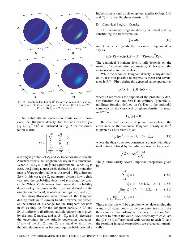
Fig. 2. Bingham densities on S2 for varying values of Z1 and Z2.(a) Z1 =¡100, Z2 = 0. (b) Z1 =¡100, Z2 =¡10. (c) Z1 =¡25,

Z2 = 0. (d) Z1 =¡25, Z2 =¡10.

No valid attitude quaternion exists on S2; how-ever, the Bingham density for the unit vector q=

[x1 x2 x3]T 2 S2 is illustrated in Fig. 2 for the orien-

tation matrix

M=

266664p2

2

p2

20

0 0 1p2

2¡p2

20

377775and varying values of Z1 and Z2 to demonstrate how the

Z matrix affects the Bingham density in this dimension.

When Z1 = Z2 = 0, all q are equiprobable. When Z2 is

zero, the q along a great circle defined by the orientation

matrixM are equiprobable, as observed in Figs. 2(a) and

2(c). In this case, the Z1 parameter dictates how tightly

clustered the probability density of q is along the great

circle. When Z2 decreases from zero, the probability

density of q increases in the direction defined by the

orientation matrixM, as observed in Figs. 2(b) and 2(d).

No straightforward visualization of the Bingham

density exists in S3. Similar trends, however, are presentas the entries of Z change for the Bingham densities

in S3 as they do for the Bingham density in S1 andS2. A uniformly distributed attitude quaternion is givenby the null Z matrix, and as Z1, Z2, and Z3 decrease,

the uncertainty in the attitude quaternion decreases.

If any of the Z1, Z2, and Z3 are equal to zero, then

the attitude quaternion becomes equiprobable around a

higher-dimensional circle or sphere, similar to Figs. 2(a)

and 2(c) for the Bingham density in S2.

D. Canonical Bingham Density

The canonical Bingham density is introduced by

substituting the transformation

q=Mp (16)

into (13), which yields the canonical Bingham den-

sity as

pb(p;Z) = pb(p;I,Z) = F¡1(Z)expfpTZpg:

The canonical Bingham density still depends on the

matrix of concentration parameters, Z; however, the

elements of p are uncorrelated.

While the canonical Bingham density is only defined

on Ss, it is still possible to express its mean and covari-ance in Rs+1. First, define the expected value operator as

Epff(x)g=Z−

f(x)p(x)dx,

where − represents the support of the probability den-

sity function p(x) and f(x) is an arbitrary (potentially)

nonlinear function defined on −. Due to the antipodalsymmetry of the canonical Bingham density, its mean

in Rs+1 isEpbfpg= 0:

Because the elements of p are uncorrelated, the

covariance of the canonical Bingham density in Rs+1is given by (2.9) from [8] as

EpbfppTg= diag[f1 f2 ¢ ¢ ¢fs+1], (17)

where the diagv operator constructs a matrix with diag-

onal entries defined by the arbitrary row vector v and

fi¢=F¡1(Z)

@F(Z)

@Zi:

The fi terms satisfy several important properties, given

by

s+1Xi=1

fi = 1 (18a)

fi > 0, i= 1,2, : : : ,s+1 (18b)

limZi!¡1

fi = 0+, i= 1,2, : : : ,s (18c)

limZ1,Z2,:::,Zs!¡1

fs+1 = 1¡: (18d)

These properties will be exploited when determining the

weights of sigma points of the unscented transform for

the canonical Gauss-Bingham density in Section V-B.

In order to obtain the @F(Z)=@Zi necessary to calculate

the fi, (14) is differentiated with respect to each Zi, and

the resulting integral expressions are evaluated numeri-

cally.

UNCERTAINTY PROPAGATION OF CORRELATED QUATERNION AND EUCLIDEAN STATES 191

E. Mean and Covariance of the Bingham Density

Like the canonical Bingham density, the mean of the

Bingham density is given in Rs+1 as

Epbfqg= 0due to antipodal symmetry. The covariance of the Bing-

ham density in Rs+1 is defined by EpbfqqTg. In order to

calculate this expected value, its argument is first pre-

and post-multiplied by MMT = I, such that the covari-

ance can be expressed as

EpbfqqTg= EpbfMMTqq

TMMTg: (19)

Introducing the transformation of variables defined in

(16) and noting that M is deterministic, (19) can be

expressed as

EpbfqqTg=MEpbfpp

TgMT: (20)

EpbfppTg is simply the covariance of the canonical

Bingham density, which is defined by (17). Substituting

(17) into (20) yields the covariance of the Bingham

density in Rs+1 as

EpbfqqTg=Mdiag[f1 f2 ¢ ¢ ¢fs+1]MT,

which is seen to be a similarity transformation of the

covariance of the canonical Bingham density according

to the orientation matrix of the Bingham density.

IV. GAUSS-BINGHAM DENSITY

The Gauss-Bingham density quantifies a state vec-

tor composed of a Gaussian-distributed vector, x 2 Rr,and a Bingham-distributed unit vector, q 2 Ss, on itsnatural manifold defined by Rr£Ss. Before construct-ing the Gauss-Bingham density, first consider the mo-

tivating example of manipulating two jointly Gaussian-

distributed random vectors given by x and y into the

product of the density of x and the density of y condi-

tioned on x. The joint density of [xT yT]T is Gaussian

and is given by

pg

÷x

y

¸;

·mx

my

¸,

"Px Pxy

PTxy Py

#!,

where m and P represent the mean and covariance of

their subscripted vector(s), respectively. The density of

y conditioned on x is Gaussian-distributed and is given

by [23]

pg(y j x;myjx(x),Pyjx)= pg(y j x;my +PTxyP¡1x (x¡mx),Py ¡PTxyP¡1x Pxy),

where myjx(x) and Pyjx are the mean and covariance,respectively, of y conditioned on x. It is interesting to

note the functional dependence of myjx on x. From the

definition of conditional probability, it follows that the

joint density of x and y can be expressed as

pg

÷x

y

¸;

·mx

my

¸,

"Px Pxy

PTxy Py

#!= pg(x;mx,Px)

£pg(y j x;my +PTxyP¡1x (x¡mx),Py ¡PTxyP¡1x Pxy): (21)

The conditional mean and covariance of p(y j x) are notrestricted to be

myjx(x) =my +PTxyP

¡1x (x¡mx) (22a)

Pyjx = Py ¡PTxyP¡1x Pxy (22b)

for the definition of conditional probability to be valid;

however, (22) must hold for the result to be Gaussian-

distributed.

The left- and right-hand sides of (21) express the

joint Gaussian density of [xT yT]T in two different

forms. In the case where the vectors x and y are jointly

Gaussian-distributed, as they are in this example, little

if anything is gained by manipulating the left-hand side

of (21) into the ride-hand side of (21); however, in the

case when one or both of the jointly distributed vectors

are not Gaussian-distributed, correlation between the

vectors can be introduced in a similar fashion to (21) by

utilizing the definition of conditional probability. This

allows the density of two jointly distributed random

vectors, x1 and x2, to be written as the product of the

density of x1 and the density of x2 conditioned on x1; i.e.

p(x1,x2) = p(x1)p(x2 j x1):Using the definition of conditional probability, the

Gauss-Bingham density is constructed as the product of

a Gaussian density and a Bingham density conditioned

on the Gaussian-distributed random variable as

pgb(x;m,P,M(z),Z)¢=pg(x;m,P)pb(q;M(z),Z), (23)

where x= [xT qT]T. The Bingham density is condi-

tioned on the Gaussian-distributed random variable xthrough the orientation matrix M(z) using the transfor-mation of variables that defines the canonical Gaussian

density, which is given by (12). The orientation matrix

is expressed using z (the random variable correspondingto the canonical Gaussian density) instead of x for bet-ter numerical stability since z is nondimensional. Thefunctional dependence of the orientation matrix on z isdiscussed in Section IV-A.

The Gauss-Bingham density possesses the following

favorable properties for probabilistically quantifying the

attitude quaternion (when s= 1 or s= 3) and other

Euclidean states:

– The Gauss-Bingham density is antipodally symmet-

ric in the attitude quaternion; thus, antipodal quater-

nions q and ¡q (which represent the same physicalattitude) are equiprobable,

192 JOURNAL OF ADVANCES IN INFORMATION FUSION VOL. 11, NO. 2 DECEMBER 2016

Fig. 3. Gauss-Bingham densities on R1 £S1 for a linear andquadratic correlation structure. (a) Linear correlation. (b) Quadratic

correlation. (c) Marginalized quaternion. (d) Marginalized

quaternion.

– the Gauss-Bingham density quantifies the uncer-

tainty of Euclidean states and the attitude quaternion

on their natural manifold Rr£Ss, and– the Gauss-Bingham density possesses a simple rep-

resentation of an equiprobable attitude quaternion

for a given angular velocity when the Z matrix is

null.

In order to illustrate these properties, consider an

application of the Gauss-Bingham density to quantify

the uncertainty of the one-dimensional attitude quater-

nion and angular velocity of a body undergoing rota-

tion about the z-axis. In this case, the state vector is

defined as

x=

·! 2R1q 2 S1

¸2 R1£S1, (24)

where ! is the angular velocity about the z-axis and q

is the one-dimensional attitude quaternion of the body,

which is defined by (15). No correlation structure for

the orientation matrix, M(z), has yet been defined. Be-fore formally defining this correlation structure, first

consider two types of correlation, which are introduced

into a set of parameters used to specify M(z): linearand quadratic. Figs. 3(a) and 3(b) show examples of

the Gauss-Bingham density (with Z1 6= 0) for the lin-ear and quadratic correlation structures, respectively.

The marginalized attitude quaternion for the linear and

quadratic correlation structures are shown in Figs. 3(c)

and 3(d), respectively. It can be observed in these figures

that the probability of the antipodal attitude quaternions

is equal for any given angular velocity, which is a de-

sirable property as these quaternions represent the same

physical attitude.

When Z= 0, the marginalized attitude quaternionis equiprobable regardless of the correlation structure

Fig. 4. Gauss-Bingham density on R1£S1 for Z1 = 0.(a) Gauss-Bingham density. (b) Marginalized quaternion.

used. This is illustrated in Figs. 4(a) and 4(b), which

show the Gauss-Bingham density in R1£S1 and themarginal density of the attitude quaternion when Z1 = 0.

This property of the Gauss-Bingham density is ad-

vantageous for representing the attitude quaternion as

equiprobable when no prior attitude information is

available.

A. Correlation Structure

In order to define the correlation structure for the

orientation matrix M(z), it is important to note thatM(z) 2 SO(s+1) 8z 2 Rr. In order to ensure that thiscondition is met, the correlation structure is introduced

into a minimum set of parameters necessary to spec-

ify the orientation matrix, denoted by Á(z), such thatthe orientation matrix is given by M(Á(z)). A minimum

parameter set, which is comprised of s(s+1)=2¢=nÁ

parameters, is necessary to define the orientation ma-

trix; therefore Á(z) 2Rs(s+1)=2 [24], [25]. The methodfor constructing the orientation matrix from the set of

minimum parameters depends on s and the parameter set

chosen. Methods for constructing the orientation matrix

for dimensions s= 1,2,3 are presented in this section.

1) s= 1: First consider the Gauss-Bingham density

specialized to s= 1. Only one parameter is necessary to

specify the orientation matrix in this dimension since

nÁ = 1. This parameter is chosen to be the magnitude

of the rotation about the known axis of rotation, which

is given by μ(z), such that Á(z) = μ(z). The orientationmatrix is then defined by

M(Á(z)) =M(μ(z)) =·cosμ(z) sinμ(z)

¡sinμ(z) cosμ(z)

¸:

The angle of rotation, μ(z), is defined on the interval[¡¼,¼) for all z. Since M(μ(z)) =M(μ(z) +2¼k) for allk 2 Z, where Z is the set of integers, μ(z) can be boundedto the interval [¡¼,¼) for all z by adding the appropriatemultiple of 2¼.

2) s= 2: Now consider the Gauss-Bingham density

specialized to s= 2. Three parameters are necessary to

specify the orientation matrix in this dimension. These

parameters are chosen to be the rotation vector, such

UNCERTAINTY PROPAGATION OF CORRELATED QUATERNION AND EUCLIDEAN STATES 193

that Á(z) = μ(z). The orientation matrix is then givenby (6) as

M(Á(z)) =M(μ(z)) = I¡ sinkμ(z)k·μ(z)kμ(z)k£

¸

+(1¡ coskμ(z)k)·μ(z)kμ(z)k£

¸2:

If kμ(z)k= 0, M(z) = I, since the angle of rotation iszero. The norm of the rotation vector, kμ(z)k, is de-fined on the interval [¡¼,¼) for all z. Since M(μ(z)) =M(μ(z) +2¼kμ(z)=kμ(z)k) for all k 2 Z, kμ(z)k can bebounded to the interval [¡¼,¼) for all z by adding theappropriate multiple of 2¼μ(z)=kμ(z)k.3) s= 3: Finally, consider the Gauss-Bingham den-

sity specialized to s= 3. Six parameters are necessary to

specify the orientation matrix in this dimension. These

parameters are chosen to be two rotation vectors repre-

senting a left- and right-isoclonic rotation [26]. Let these

rotation vectors be denoted by μL(z) and μR(z), respec-tively, such that Á(z) = [μTL (z) μ

TR(z)]

T. The orientation

matrix is then defined using left- and right-isoclonic ro-

tations according to

M(Á(z)) =Mμ·

μL(z)

μR(z)

¸¶= L(q(μL(z)))R(q(μR(z))),

where

L(q) =

26664q ¡qx ¡qy ¡qzqx q ¡qz qy

qy qz q ¡qxqz ¡qy qx q

37775

R(q) =

26664q ¡qx ¡qy ¡qzqx q qz ¡qyqy ¡qz q qx

qz qy ¡qx q

37775 ,and q(μL(z)) and q(μR(z)) are defined by (7). The normof each of these rotation vectors, kμL(z)k and kμR(z)k,is defined on the interval [¡¼,¼) for all z. Since

M

μ·μL(z)

μR(z)

¸¶=M

μ·μL(z) +2¼kLμL(z)=kμL(z)kμR(z)+2¼kRμR(z)=kμR(z)k

¸¶for all kL,kR 2 Z, kμL(z)k and kμR(z)k can be boundedto the interval [¡¼,¼) for all z by adding the appropriatemultiple of 2¼μL(z)=kμL(z)k and 2¼μR(z)=kμR(z)k toμL(z) and μR(z), respectively.Now that the functional dependence of the orien-

tation matrix, M(Á(z)), on the minimal set of param-eters, Á(z), has been defined for s= 1,2,3, the func-tional dependence of Á(z) on z needs to be defined.Two choices for this functional dependence are consid-

ered: linear and quadratic. It is noted that the quadratic

form of this functional dependence is not used after it is

presented; however, it is a valid form of this functional

dependence and is presented to show the flexibility of

the Gauss-Bingham density.

First, consider the quadratic dependence of Á(z) onz, which is defined by

Á(z) = Á0 +¯z

+[zT¡1z zT¡2z ¢ ¢ ¢zT¡nÁz]T, (25)

where Á0 2RnÁ , ¯ 2 RnÁ£r and ¡i 2 fRr£r : ¡i = ¡Ti g,i= 1, : : : ,nÁ quantify the zeroth-, first-, and second-order

correlation, respectively, of z on Á(z). The choice ofimplementing z instead of x in the correlation structureresults in nondimensional coefficients ¯ and ¡i, whichis preferred for numerical stability. Noting that the

orientation matrix M(z) is now explicitly defined by

z, Á0, ¯, ¡1, : : : ,¡nÁ and that z is explicitly defined byx, m, and P, the orientation matrix using the quadraticcorrelation structure is parameterized as

M(z) =M(x;m,P,Á0,¯,¡1, : : : ,¡nÁ),

and the Gauss-Bingham density is given by the special-

ization of (23) as

pgb(x;m,P,Á0,¯,¡1, : : : ,¡nÁ ,Z) =

pg(x;m,P)pb(q;M(x;m,P,Á0,¯,¡1, : : : ,¡nÁ),Z):

The number of parameters necessary to quantify the

quadratic correlation between z and Á(z) is 12nÁ(2+2r+

r(r+1)), which increases quadratically with r. For one-

dimensional attitude (R1£S1), three-dimensional atti-tude (R3£S3), and dynamic pose (R9£S3) quantifica-tion, 3, 60, and 330 unique parameters are needed to

quantify the quadratic relationship between Á(z) and z.Now, consider the linear correlation structure for

Á(z), which is given by a simplification of (25) as

Á(z) = Á0 +¯z:

Using the linear correlation structure, the orientation

matrix is parameterized as

M(z) =M(x;m,P,Á0,¯),

and the Gauss-Bingham density is given by the special-

ization of (23) as

pgb(x;m,P,Á0,¯,Z)

= pg(x;m,P)pb(q;M(x;m,P,Á0,¯,Z):

The number of parameters necessary to quantify the lin-

ear correlation between z and Á(z) is nÁ(1+ r), whichincreases linearly with r. For one-dimensional attitude,

three-dimensional attitude, and dynamic pose quantifi-

cation, 2, 24, and 60 unique parameters are needed to

quantify the linear relationship between Á(z) and z. Be-cause the number of parameters necessary to quantify

the linear correlation between z and Á(z) increases lin-early (as opposed to quadratically) with r, it is used in

the remainder of this work.

194 JOURNAL OF ADVANCES IN INFORMATION FUSION VOL. 11, NO. 2 DECEMBER 2016

B. Canonical Gauss-Bingham Density

The canonical Gauss-Bingham density is introduced

by substituting the transformations

x= Sz+m and q=M(z)p (26)

into (23), which yields the canonical Gauss-Bingham

density aspgb(z;Z) = pg(z)pb(p;Z),

where z= [zT pT]T. The elements of z are uncorrelatedand zero mean, such that the covariance of z is defined

by I and (17) and is given by

EpgbfzzTg= diag[1 ¢ ¢ ¢1 f1 ¢ ¢ ¢fs+1]: (27)

V. UNCERTAINTY PROPAGATION

In order to propagate the uncertainty of a given

Gauss-Bingham-distributed state vector, an unscented

transform is used and the weighted maximum log-

likelihood parameters of the Gauss-Bingham density are

found. The unscented transform generates a set of deter-

ministically chosen sigma points that represent the given

Gauss-Bingham density. Each sigma point is then trans-

formed according to known (potentially) nonlinear sys-

tem dynamics. The weighted maximum log-likelihood

parameters of the propagated Gauss-Bingham density

are then recovered from the transformed sigma points.

A. System Dynamics

Assume that discrete-time nonlinear system dynam-

ics are given byxk = f(xk¡1), (28)

where x= [xT qT]T, and define the state vector withthe antipodal attitude quaternion as x= [xT ¡ qT]T. Be-cause q quantifies an antipodally equivalent attitude rep-

resentation in which q and ¡q represent the same phys-ical attitude, the antipodal symmetry of q must be pre-

served by the system dynamics; that is, if

xk = f(xk¡1) and xk = f(xk¡1), (29)

then the quaternion elements of xk and xk remain an-

tipodal. Equation (29) defines an important property of

the system dynamics, f. This property states that the

system dynamics preserve the antipodal symmetry of

the quaternion, which is exploited to reduce the amount

of computation necessary to propagate the sigma points

representing the Gauss-Bingham density.

B. Unscented Transform

In order to select a set of weights and locations

for the sigma points of the unscented transform for the

canonical Gauss-Bingham density, the zeroth, first, and

second moments between the canonical Gauss-Bingham

density and the sigma points are matched in Rr£Rs+1.The moments will be matched in Rr£Rs+1; however,the sigma points will be parameterized such that they

remain on the manifold Rr£Ss. After finding sigma

points for the canonical Gauss-Bingham density, (26)

is then used to convert the locations of the sigma points

from the canonical Gauss-Bingham to the given Gauss-

Bingham density.

In order to reduce the number of sigma points, only

one of each pair of antipodal sigma points is considered

and propagated since the system dynamics preserve the

antipodal symmetry of the sigma points as shown by

(29). To illustrate this concept, consider the following

example antipodal sigma points in R1£S1 at tk¡1, Xk¡1and Xk¡1, that are antipodal in q and given by

Xk¡1 =·3

1p2

¡1p2

¸Tand

Xk¡1 =·3

¡1p2

1p2

¸T:

These sigma points are propagated by some (poten-

tially) nonlinear function, f, that satisfies the property

given by (29). Assume that this propagation transforms

the sigma points to

Xk = [4 0 1]T and Xk = [4 0 ¡ 1]T,which are still antipodal in q; thus, the computational

expense can be lowered by considering only Xk¡1. Xk¡1is transformed according to f to obtainXk, and antipodalsymmetry can be used to obtain Xk, if desired.In order to generate the sigma points for the Gauss-

Bingham density, motivation is drawn from the 2n+1

unscented transform. The 2n+1 unscented transform

for the canonical Gaussian density places two sigma

points at equal but opposite deviations from zero for

each of the n= r canonical Gaussian states. A central

sigma point is then placed at the origin. When generat-

ing sigma points for the canonical Gauss-Bingham den-

sity, which considers only one of each pair of antipodal

points in the attitude quaternion, a similar approach to

that of the 2n+1 unscented transform for the canonical

Gaussian density is used.

In order to generate the sigma points for the canon-

ical Gauss-Bingham density, first a set of sigma points

that quantify deviations from the origin in each state

of z are introduced as §± while p is held constant asthe identity quaternion. The locations of these 2r sigma

points are given by

Z (1),(2) = [

2Rrz }| {§± 0 ¢ ¢ ¢0

2Ssz }| {0 ¢ ¢ ¢0 1]T

Z (3),(4) = [0 § ± ¢ ¢ ¢0 0 ¢ ¢ ¢0 1]T

...

Z(2r¡1),(2r) = [0 ¢ ¢ ¢0 § ± 0 ¢ ¢ ¢0 1]T,

with corresponding weights given by

w(1),(2) = w(3),(4) = ¢ ¢ ¢= w(2r¡1),(2r) = wg4r,

UNCERTAINTY PROPAGATION OF CORRELATED QUATERNION AND EUCLIDEAN STATES 195

where Z (i),(j) and w(i),(j) represent the locations and

weights of the ith and jth sigma points, respectively,

representing the canonical Gauss-Bingham density and

wg is a parameter used to specify the weights of these

sigma points. The braces are used to denote the portions

of Z which are the Euclidean and quaternion states,

respectively.

Next, angular deviations are introduced into the

quaternion state as §®` for `= 1,2, : : : ,s while z is heldconstant at zero in order to guarantee that the perturbed

attitude quaternion remains on the unit hypersphere.

These 2s sigma points are given by

Z(2r+1),(2r+2) = [

2Rrz }| {0 ¢ ¢ ¢0

2Ssz }| {§S®1 0 ¢ ¢ ¢0 C®1 ]

T

Z(2r+3),(2r+4) = [0 ¢ ¢ ¢0 0 § S®2 ¢ ¢ ¢0 C®2 ]T

...

Z(2r+2s¡1),(2r+2s) = [0 ¢ ¢ ¢0 0 ¢ ¢ ¢0 § S®s C®s]T,

with corresponding weights given by

w(2r+1),(2r+2) =wb14

w(2r+3),(2r+4) =wb24

...

w(2r+2s¡1),(2r+2s) =wbs4,

where wb` , for `= 1,2, : : : ,s, are parameters used to

specify the weights of these sigma points and S® and

C® represent the sine and cosine of ®, respectively.

Finally, a central sigma point is placed at z= 0and in the “zero” direction of p, which is the identity

quaternion. This single sigma point is given by

Z (N) = [

2Rrz }| {0 ¢ ¢ ¢0

2Ssz }| {0 ¢ ¢ ¢0 1]T,

with corresponding weight given by

w(N) =wc2,

where wc is a parameter used to specify the weight of

this sigma point and N = 2r+2s+1 is the total number

of sigma points.

In order to find the parameters ±, ®`, wc, wg, and

wb` , where `= 1,2, : : : ,s, which fully define the weights

and locations of the sigma points for the canonical

Gauss-Bingham density, the zeroth, first, and second

moments between the sigma points and the canonical

Gauss-Bingham density are matched. The zeroth and

first moments of the canonical Gauss-Bingham are 1

and 0, respectively. The second moment of the canonicalGauss-Bingham density is given by (27). While only

one of each antipodal pair of sigma points is stored

and propagated, it is important to note that both of the

antipodal sigma points, which are equally weighted, are

considered when calculating the moments of the sigma

points. After accounting for the antipodal symmetry

of each of the sigma points, the first moment of the

sigma points is zero for any choice of the parameters.

Matching the zeroth and second moments of the sigma

points with the canonical Gauss-Bingham density yields

sX`=1

wb` +wc+wg = 1 (30a)

±2wg

r= 1 (30b)

wb` sin2®` = f , `= 1,2, : : : ,s (30c)

sX`=1

wb` cos2®`+wc+wg = fs+1, (30d)

where (30a) stems from the zeroth moment and (30b)—

(30d) stem from the second moment. Summing (30c)

for `= 1,2, : : : ,s and (30d) while noting the properties

in (18) yields (30a); thus, (30d) is redundant and may

be neglected. Solving (30b) and (30c) for ± and ®` gives

the locations of the sigma points as a function of their

weights as

± =

sr

wgand ®` = asin

sf

wb`, (31)

where `= 1,2, : : : ,s. Now, the weights must be selected

for the sigma points. In order for (31) to have real

solutions, wb` must be greater than or equal to f for

all `= 1,2, : : : ,s. In order to ensure that this condition

is met, a somewhat nonintuitive choice for the weights

of the sigma points for the canonical Gauss-Bingham

density is chosen that parallels the choice of weights of

the sigma points for the Bingham density presented in

[12]. Noting the properties given in (18), the weights

of the sigma points representing the Gauss-Bingham

density which satisfy (30a) are chosen as

wb` = f +(1¡¸¡·)fs+1s, `= 1,2, : : : ,s (32a)

wc = ¸fs+1 (32b)

wg = ·fs+1, (32c)

where ¸ and · are positive tuning parameters such that

¸+· < 1. While choosing the weights according to (32)

is nonintuitive, this choice of weights satisfies (30a) and

provides real locations for the sigma points. ¸ and · are

chosen such that the weights of all the sigma points

approach an equal weight of 1=N as the uncertainty in

the states corresponding to q approaches zero; that is,

Z1,Z2, : : : ,Zs!¡1. This choice of weights ensures thatthe sigma points possess nearly equal weights, and thus

have nearly equal importance, when the uncertainty in

the attitude quaternion is small. Using the properties in

(18), the ¸ and · that yield equal weights for the sigma

196 JOURNAL OF ADVANCES IN INFORMATION FUSION VOL. 11, NO. 2 DECEMBER 2016

points as the uncertainty in the quaternion goes to zero

are given by

¸=1

Nand ·=

2r

N: (33)

The sigma points on the canonical Gauss-Bingham den-

sity, which are defined in terms of the parameters in

(31), (32), and (33), are transformed from the canonical

Gauss-Bingham density to the Gauss-Bingham density

of interest defined by pgb(x;m,P,Á0,¯,Z) according to

(26). These transformed sigma points and their associ-

ated weights are denoted by X (i) and w(i), respectively,

where i= 1,2, : : : ,N.

The sigma points representing the Gauss-Bingham

density at tk¡1, Xk¡1, are then transformed according tothe nonlinear system dynamics given by (28) to obtain

the sigma points representing the Gauss-Bingham den-

sity at tk, Xk. If the dynamical system is governed by

continuous-time dynamics, the nonlinear discrete-time

function in (28), f, is given by the integration of xk¡1from tk¡1 to tk to obtain xk.

C. Maximum Weighted Log-LikelihoodGauss-Bingham Parameters

In order to obtain the parameters of the best-fit

Gauss-Bingham density given the set of sigma points

and weights at tk, the parameters of the Gauss-Bingham

density that maximize the weighted log-likelihood of the

sigma points are found. To illustrate why the maximum

weighted log-likelihood parameters are sought, consider

the case when the unscented transform is used for a state

that exists in Rr. Given the sigma points and weightsfrom the unscented transform, the mean and covariance

are recovered from the weighted sample mean and

covariance of the sigma points. It can be shown that

the weighted sample mean and covariance of the sigma

points is the mean and covariance of the Gaussian

density that maximizes the weighted log-likelihood of

the sigma points.

In this spirit, the parameters of the Gauss-Bingham

density are recovered from the sigma points accord-

ing to

mk,Pk,Á0,k,¯k,Zk =

argmaxm,P,Á0,¯,Z

NXi=1

w(i) lnpgb(X (i)k ;m,P,Á0,¯,Z): (34)

This maximization can be performed analytically for

the mean and covariance of the Gaussian density, m

and P. First, note that the sigma points can be decom-

posed into their Euclidean and quaternion portions ac-

cording to Xk = [X Tx,k X T

q,k]T. The mean and covariance

of the Gaussian density that maximizes the weighted

log-likelihood of the sigma points is given by the sam-

ple mean and covariance of the Euclidean portion of the

sigma points according to

mk = 2

NXi=1

w(i)X (i)x,k (35a)

Pk = 2

NXi=1

w(i)(X (i)x,k ¡mk)(X (i)

x,k ¡mk)T, (35b)

where the factor of two is included since only one of

each antipodal pair of sigma points in the quaternion

state is quantified.

After using (35) to determine mk and Pk, (34) be-

comes

Á0,k,¯k,Zk = argmaxÁ0,¯,Z

J(Á0,¯,Z), (36)

where

J(Á0,¯,Z) =NXi=1

w(i) lnpgb(X (i)k ;mk,Pk,Á0,¯,Z):

This maximization is carried out numerically to find Á0,¯, and Z. In order to perform this numerical maximiza-

tion, it is first transformed into a root-finding problem

according to the first derivative conditions of a maxi-

mum, i.e.

@J(Á0,k,¯k,Zk)

@Á0,k= 0 (37a)

@J(Á0,k,¯k,Zk)

@¯k= 0 (37b)

@J(Á0,k,¯k,Zk)

@Zk= 0, (37c)

where the explicit expressions for the derivatives are

omitted for brevity. A root-finding algorithm is used to

find the Á0,k, ¯k, and Zk that satisfy (37). To initializethe root-finding algorithm, Á0,k¡1, ¯k¡1, and Zk¡1 areused. By initializing the root-finding algorithm in this

way, if the propagation time step is chosen sufficiently

small, Á0,k¡1, ¯k¡1, and Zk¡1 remain close to the localmaximum and a gradient-based root-finding algorithm

will converge to Á0,k, ¯k, and Zk without excessiveiteration required or risk of diverging to a different root.

A number of root-finding algorithms can be used

to find the Á0,k, ¯k, and Zk that satisfy (37). The

Levenberg-Marquardt algorithm, a well-known opti-

mizer, is chosen to find these Á0,k, ¯k, and Zk [27], [28].This algorithm is used to find the roots of an arbitrary

system of equations defined by g(x) = 0 by minimizingthe cost function gT(x)g(x) using x as the minimization

variable. The Levenberg-Marquardt algorithm was cho-

sen to find Á0,k, ¯k, and Zk since the cost function willremain near the minimum if the time step is chosen

sufficiently small and Á0,k¡1, ¯k¡1, and Zk¡1 are used

UNCERTAINTY PROPAGATION OF CORRELATED QUATERNION AND EUCLIDEAN STATES 197

to initialize the algorithm. Applying the Levenberg-

Marquardt algorithm in this manner to find the roots

of (37) was found to be more computationally efficient

than applying it to the optimization problem in (36) di-

rectly.

D. Uncertainty Propagation Algorithm

In summary, the algorithm used to propagate the

Gauss-Bingham density is given by

– Given:

– A Gauss-Bingham-distributed state vector at t0defined by pgb(x;m0,P0,Á0,0,¯0,Z0).

– System dynamics that preserve the antipodal

symmetry of the quaternion as defined by the

property given by (29).

– A sequence of times to which to propagate the

Gauss-Bingham density, t1, t2, : : : , tf .

1) Generate the sigma points and weights according to

pgb(x;m0,P0,Á0,0,¯0,Z0).

2) Set the time counter to k = 1

3) Propagate the sigma points from tk¡1 to tk accordingto the given system dynamics.

4) Recover mk and Pk according to (35).

5) Recover Á0,k, ¯k, and Zk according to the root-

finding problem defined by (37) using Á0,k¡1 ,¯k¡1,and Zk¡1 to initialize the root-finding algorithm.

6) If tk = tf , stop; if tk < tf , set k = k+1 and return to

step 3.

The sequence of times to which to propagate the

Gauss-Bingham density, t1, t2, : : : , tf , should be chosen

such that the time step is small enough that Á0,k¡1, ¯k¡1,and Zk¡1 are close to Á0,k, ¯k, and Zk in order to ensurethat the root-finding algorithm converges to the proper

solution for Á0,k, ¯k, and Zk. The size of the time step isa compromise between computational cost and ensuring

that the root-finding algorithm converges to the correct

root. Because the sigma points are not resampled at

each time step, no approximation error is introduced

by choosing the time step too small. Since the time

step chosen is problem dependent, general guidelines

for choosing this time step can not be imposed.

VI. SIMULATIONS

Two simulations are performed to illustrate uncer-

tainty propagation using the Gauss-Bingham density.

The first simulation propagates the uncertainty of the

planar attitude and angular velocity of a body in R1£S1,where the Gauss-Bingham density can be visualized on

the unit cylinder. This simulation provides an intuitive

example of uncertainty propagation using the Gauss-

Bingham density. The second simulation propagates the

uncertainty in the dynamic pose (position, velocity, at-

titude, and angular velocity) of a chase spacecraft with

respect to a target spacecraft. This simulation com-

pares uncertainty propagation using the Gauss-Bingham

density to the predictor of the multiplicative extended

Kalman filter and a Monte Carlo approach in order to

show the efficacy of uncertainty propagation using the

Gauss-Bingham density.

A. Planar Attitude and Angular Velocity

Consider the attitude quaternion and angular veloc-

ity representing the one-dimensional attitude motion of

a body undergoing rotation about the z-axis. In this case,

the state vector of the body is defined by (24). The an-

gular velocity comprises the Gaussian-distributed por-

tion of the state vector, with initial mean and covariance

given by

m0 = 0 and P0 = (0:01±=s)2, (38)

respectively. The attitude quaternion comprises the con-

ditional Bingham-distributed portion of the state vector,

and is initially uncorrelated with the angular velocity

(that is, ¯0 = 0). The parameters defining the orien-tation and concentration of the conditional Bingham-

distributed portion of the state vector are given by

Á0 = 0 and Z1,0 =¡100,respectively. The Gauss-Bingham density representing

the initial attitude quaternion and angular velocity of

the body, as well as the sigma points generated by

the unscented transform, are shown in Fig. 5(a). The

marginalized density of the initial attitude quaternion is

shown in Fig. 5(c).

The body undergoes torque-free motion, that is,

¿B = 0. The temporal evolution of the attitude quater-nion and angular velocity are given by (9) and (10), re-

spectively. The uncertainty propagation algorithm sum-

marized in Section V-D is used to propagate the uncer-

tainty of the attitude quaternion and angular velocity

forward in time. A time step of one minute is used

to propagate the uncertainty, which is small enough

to ensure that the root-finding algorithm converges to

the proper Á0,k, ¯k, and Zk at each time step. Fig.5 shows the evolution of Gauss-Bingham density and

sigma points representing the attitude quaternion and

angular velocity of the body, as well as the marginal-

ized density of the attitude quaternion over time. Table

I provides the corresponding parameters of the Gauss-

Bingham density over time. It is observed that the mean

and covariance of the angular velocity, m and P, respec-

tively, remain constant, which is expected since (10)

shows that the angular-velocity is constant under torque-

free motion.

The concentration parameter of the conditional Bing-

ham density, Z, remains constant (within numerical ac-

curacy of the root finding algorithm). The mean di-

rection of the Gauss-Bingham density, Á0, remains atzero since the mean of the angular velocity is zero for

all time; however the linear correlation parameter, ¯evolves in time in order to quantify the effect of the

uncertain angular velocity on the attitude quaternion.

198 JOURNAL OF ADVANCES IN INFORMATION FUSION VOL. 11, NO. 2 DECEMBER 2016

Fig. 5. Gauss-Bingham uncertainty propagation for

one-dimensional attitude motion. (a) Initial state density. (b) State

density at 15 minutes. (c) Initial quaternion density. (d) Quaternion

density at 15 minutes. (e) State density at 1 hour. (f) State density at

6 hours. (g) Quaternion density at 1 hour. (h) Quaternion density at

6 hours.

TABLE I

Gauss-Bingham Parameters over time

Time [hours] m [±=s] P [(±=s)2] Á0 ¯ Z1

0 0 (0:01)2 0 0.0000 ¡1000.25 0 (0:01)2 0 0.0785 ¡1001 0 (0:01)2 0 0.3142 ¡1006 0 (0:01)2 0 1.8850 ¡100

It is interesting to note that ¯ evolves linearly in timefor this problem. The Gauss-Bingham density eventu-

ally wraps around its cylindrical manifold as it is prop-

agated, which causes the attitude quaternion to become

equiprobable as time increases, and is apparent in Fig.

5(h). This is an expected result for a body undergoing

one-dimensional attitude motion with an uncertain an-

gular velocity; as time increases, the uncertainty in the

attitude quaternion of the body grows until the attitude

quaternion becomes equiprobable.

Several important properties of the Gauss-Bingham

density and its utility in uncertainty propagation can be

observed in Fig. 5. The Gauss-Bingham density is an-

tipodally symmetric in the quaternion state for all time,

which is a necessary property to properly quantify the

uncertainty in the attitude quaternion. Since this exam-

ple quantifies the one-dimensional attitude motion in

R1£S1, N = 5 sigma points are required to quantify thetemporal evolution of the Gauss-Bingham density. The

attitude quaternion becomes equiprobable as the uncer-

tainty is propagated; however, the concentration param-

eter Z1 does not approach zero. As the uncertainty is

propagated, the attitude quaternion becomes equiproba-

ble due to the wrapping of the Gauss-Bingham density

around the cylinder, not because the concentration pa-

rameter approaches zero.

B. Spacecraft Relative Pose

Now consider an example in which a chase space-

craft is orbiting in close proximity to a target space-

craft. The state of the chase spacecraft is defined to be

[!T ±rT ±vT qT]T, where q and ! represent the attitude

quaternion and angular velocity of the chase spacecraft,

respectively, and ±r and ±v represent the relative position

and velocity, respectively, of the chase spacecraft with

respect to the target spacecraft. The chase spacecraft

is taken to have an identity inertia tensor and under-

goes torque-free motion, with the temporal evolution

of the attitude quaternion and angular velocity given

by (9) and (10), respectively. Since the body undergoes

torque-free motion and has an identity inertia tensor,

(10) shows that the angular velocity is constant in time.

In order to quantify the temporal evolution of the

relative position and velocity, the Clohessy-Wiltshire

equations are used [29]—[31]. The Clohessy-Wiltshire

equations approximate the relative motion of the chase

spacecraft with respect to the target spacecraft under

the assumptions that the spacecraft are in close proxim-

ity and that the target spacecraft is in a circular orbit.

If these assumptions are valid, the Clohessy-Wiltshire

equations governing the temporal evolution of the rela-

tive position and velocity are

·± _r

± _v

¸=

26666666664

0 0 0 1 0 0

0 0 0 0 1 0

0 0 0 0 0 1

3n2 0 0 0 2n 0

0 0 0 ¡2n 0 0

0 0 ¡n2 0 0 0

37777777775·±r

±v

¸, (39)

where n is the mean motion of the target spacecraft

and ±r and ±v are expressed in a rotating coordinate

frame centered on the target spacecraft. The rotating

UNCERTAINTY PROPAGATION OF CORRELATED QUATERNION AND EUCLIDEAN STATES 199

coordinate frame is defined by the position and velocity

vectors of the target spacecraft. The target spacecraft

is taken to be in a geostationary orbit with an orbital

radius of 42164 km, which results in a mean motion of

the target spacecraft of 7:2920£ 10¡5 rad=s.The Gauss-Bingham density is used to quantify the

uncertainty of the state vector of the chase spacecraft.

The Gaussian portion of the Gauss-Bingham density

quantifies the uncertainty of the angular velocity, rel-

ative position, and relative velocity, with initial mean

and covariance given by

m0 =

2666666666666666664

0:5±=s

0:8±=s

1:0±=s

0

10 km

0

0

0

0

3777777777777777775

and P0 = diag

2666666666666666664

0:12 (±=s)2

0:12 (±=s)2

0:12 (±=s)2

1 m2

1 m2

1 m2

0:012 (m=s)2

0:012 (m=s)2

0:012 (m=s)2

3777777777777777775

T

,

(40)

respectively. The attitude quaternion of the chase space-

craft comprises the conditional Bingham-distributed

portion of the state vector, and is initially uncorrelated

with the angular velocity, relative position, and rela-

tive velocity (that is, ¯0 = 0). The parameters definingthe initial orientation and concentration of the condi-

tional Bingham-distributed portion of the state vector

are given by

Á0 = 0 and Z1,0 = Z2,0 = Z3,0 =¡5000,respectively.

The uncertainty propagation algorithm summarized

in Section V-D is used to propagate the uncertainty of

the angular velocity, relative position, relative velocity,

and attitude quaternion forward in time. A time step

of fifteen seconds is used to propagate the uncertainty,

which is small enough to ensure that the root-finding al-

gorithm converges to the proper Á0,k, ¯k, and Zk at eachtime step. Uncertainty propagation using the Gauss-

Bingham density is compared to two other methods of

uncertainty propagation to evaluate its efficacy: a Monte

Carlo approach and the predictor step of the multiplica-

tive extended Kalman filter (MEKF) [5], [32], [33].

100,000 Monte Carlo samples are realized from the ini-

tial Gauss-Bingham density using an acceptance sam-

pling method, and are propagated forward in time to

quantitatively represent the true evolution of the initial

Gauss-Bingham density.

The predictor step of the MEKF quantifies the

“mean” using the attitude quaternion and relies on a

small angle assumption to project the uncertainty in the

attitude quaternion into a three parameter attitude rep-

resentation (the rotation vector is used in this analy-

sis). Quotation marks are used around “mean” for the

MEKF to indicate that it is not the mean as defined

by the first moment of the state vector; rather, it is the

“mean” quaternion as defined by one of the antipodal

pair used to quantify the quaternion estimate. In order

to find the equivalent “mean” and covariance for the

MEKF given the initial Gauss-Bingham density, it is

first noted that “mean” attitude quaternion is the iden-

tity quaternion since Á0 = 0 and ¯0 = 0; thus, the meanfor the MEKF is given by the concatenation of the mean

given in (40) and the identity quaternion. The equivalent

covariance of the MEKF state vector, which is expressed

using the rotation vector instead of the attitude quater-

nion, is found by converting the quaternion portion of

the initial Monte Carlo samples to their equivalent rota-

tion vector according to (8), and calculating their sample

covariance.

Since the angular velocity, relative position, and rel-

ative velocity are initially Gaussian-distributed, evolve

according to linear dynamics, and their temporal evolu-

tion is not a function of the attitude quaternion, they re-

main Gaussian-distributed for all time. Because of this,

both the Gauss-Bingham and MEKF uncertainty prop-

agation methods perfectly capture the evolution of the

uncertainty in these states, which is presented in Figs.

6—8 and shows the standard deviation of each compo-

nent of these states quantified by both the MEKF and

the Gauss-Bingham density over time. Furthermore, the

mean of these quantities is constant for all time since

their mean is a stationary solution to (10) and (39) un-

der torque-free motion with an identity inertia tensor.

Fig. 6 shows that the uncertainty of the angular velocity

is constant, as expected since the angular velocity is

constant. Fig. 7 shows that the uncertainty in the rel-

ative position grows as time increases. Fig. 8 shows

that the uncertainty in the x- and y-components of the

relative velocity increase, while the uncertainty in the

z-component decreases. This decrease in uncertainty is

expected due to the periodicity present in the Clohessy-

Wiltshire equations. If the uncertainty is propagated for

an entire orbit of the target spacecraft (approximately

24 hours), it would complete one cycle of its period.

Uncertainty propagation using the Gauss-Bingham

density does not require that the system dynamics gov-

erning the Gaussian-distributed states be linear nor that

their temporal evolution be functionally independent of

the attitude quaternion. These conditions are used in this

example to simplify the presentation and analysis of the

results of the uncertainty propagation. If nonlinear sys-

tem dynamics are used, or if the system dynamics are a

function of the attitude quaternion, the best-fit Gaussian

density that maximizes the weighted log-likelihood of

the sigma points as defined by (35) is found.

Because the attitude uncertainty quantified by the

Gauss-Bingham density and Monte Carlo samples are

200 JOURNAL OF ADVANCES IN INFORMATION FUSION VOL. 11, NO. 2 DECEMBER 2016

Fig. 6. Gaussian-distributed angular velocity standard deviation

quantified by the Gauss-Bingham density (black) and the MEKF

(red).

Fig. 7. Gaussian-distributed relative position standard deviation

quantified by the Gauss-Bingham density (black) and the MEKF

(red).

expressed using the attitude quaternion and the uncer-

tainty quantified by the MEKF predictor is expressed

using the rotation vector, the uncertainty quantified by

the Gauss-Bingham density and Monte Carlo samples

are converted to rotation vector space in order to make

a direct comparison. The rotation vector space is chosen

for this comparison since it is a three parameter repre-

sentation of attitude. In order to convert the uncertainty

quantified by the Gauss-Bingham density and Monte

Carlo samples from the attitude quaternion representa-

tion to the rotation vector representation, first, 100,000

samples of the Gauss-Bingham density are generated

using an acceptance sampling method. The quaternion

portion of the Gauss-Bingham samples, as well as the

Monte Carlo samples, are then converted to their equiv-

alent rotation vector according to (8). Expectation max-

imization [34] is then performed for each set of samples

to fit a Gaussian mixture density to the x-y, y-z, and x-z

projections of the rotation vector portion of the respec-

Fig. 8. Gaussian-distributed relative velocity standard deviation

quantified by the Gauss-Bingham density (black) and the MEKF

(red).

tive samples. This process is used only to visualize theuncertainty of the attitude quaternion quantified by the

Gauss-Bingham density and the Monte Carlo samples in

rotation vector space, and is not an element of the un-

certainty propagation using the Gauss-Bingham density.

Because the MEKF quantifies the mean and covariance

of the rotation vector and not its density, the density is

assumed to be Gaussian.

The attitude uncertainty quantified by the Gauss-

Bingham density, Monte Carlo samples, and MEKF at

a time of five minutes are presented in Fig. 9. Figs. 9(a)

and 9(b) show the x-y projection of the rotation vec-

tor for 1,000 of the Monte Carlo and Gauss-Bingham

samples, as well as the Gaussian mixture densities fit to

these samples to show the agreement between the sam-

ples and the densities. These plots are repeated with-

out the samples in Figs. 9(c) and 9(d) for clarity along

with the uncertainty quantified by the MEKF in red in

Fig. 9(d). Figs. 9(e) and 9(f) and Figs. 9(g) and 9(h)

show the y-z and x-z projections, respectively, of the

uncertainty quantified by the Gauss-Bingham density,

true density (as approximated from the Monte Carlo

samples), and MEKF. At the time of five minutes, the

Gauss-Bingham density agrees very well with the true

density. The MEKF quantifies the mean and covariance

of the true density as well, which is attributed to the

fact that the attitude uncertainty is still relatively small

at this time.

Fig. 10 shows the uncertainty quantified by the

Gauss-Bingham density, true density (as approximated

from the Monte Carlo samples), and MEKF at a time

of one hour in the same plots as Fig. 9. After propagat-

ing the uncertainty for one hour, the attitude uncertainty

quantified by the MEKF does not agree with the true

uncertainty, as it has outgrown the kμk 2 [¡¼,¼) boundon the rotation vector. This uncertainty can potentially

be wrapped such that it is expressed in the appropri-

ate bounded region; however, this is not common prac-

tice when using the MEKF. The underlying small angle

UNCERTAINTY PROPAGATION OF CORRELATED QUATERNION AND EUCLIDEAN STATES 201

Fig. 9. True, Gauss-Bingham (GB), and MEKF attitude

uncertainties expressed in rotation vector space at a time of five

minutes. The MEKF density is shown in red. (a) True μx-μy density

and samples. (b) GB μx-μy density and samples. (c) True μx-μydensity. (d) GB and MEKF μx-μy densities. (e) True μy-μz density.

(f) GB and MEKF μy-μz densities. (g) True μx-μz density. (h) GB

and MEKF μx-μz densities.

assumption used to derive the predictor of the MEKF

becomes invalid when the attitude uncertainties become

large; thus, it is not well-suited to propagate large atti-

tude uncertainties. This can be observed by noting that,

even if the uncertainty were wrapped to the appropriate

Fig. 10. True, Gauss-Bingham (GB), and MEKF attitude

uncertainties expressed in rotation vector space at a time of one

hour. The MEKF density is shown in red. (a) True μx-μy density and

samples. (b) GB μx-μy density and samples. (c) True μx-μy density.

(d) GB and MEKF μx-μy densities. (e) True μy-μz density. (f) GB

and MEKF μy-μz densities. (g) True μx-μz density. (h) GB and

MEKF μx-μz densities.

boundary, it still will not posses the appropriate hour-

glass shape as the true density does.

After propagating the uncertainty for one hour, the

Gauss-Bingham density is still in close agreement with

the true density as is shown in Fig. 10. This is due

202 JOURNAL OF ADVANCES IN INFORMATION FUSION VOL. 11, NO. 2 DECEMBER 2016

to the fact that the uncertainty propagation using the

Gauss-Bingham density does not rely on a small an-

gle assumption. The uncertainty is also quantified on

the natural manifold of the attitude quaternion and the

other Euclidean states, R9£S3, so the uncertainty can-not escape the bounded region on which it is defined.

Because of these reasons, uncertainty propagation us-

ing the Gauss-Bingham density remains well-suited to

quantify attitude uncertainty, even as the attitude uncer-

tainty becomes large.

VII. CONCLUSIONS

A new probability density function, called the Gauss-

Bingham density, was proposed that represents the

uncertainty of an attitude quaternion and other Eu-

clidean states of a body under a common probabilis-

tic framework. The proposed Gauss-Bingham density

is constructed as the product of a Gaussian density

and a Bingham density that is conditioned on the

Gaussian-distributed random variable, which quantifies

the correlation between the quaternion and Euclidean

states and exists on their natural manifold, Rr£Ss.The Gauss-Bingham density quantifies a uniformly-

distributed quaternion when its concentration matrix is

null, which provides a convenient method to initialize

the uncertainty when no attitude information is avail-

able. Uncertainty propagation using the Gauss-Bingham

density was presented, which leverages an unscented

transformation and recovers the maximum weighted

log-likelihood parameters of the Gauss-Bingham den-

sity from the sigma points. The Gauss-Bingham den-

sity properly quantifies the uncertainty of the attitude

quaternion and other Euclidean states without relying

on a small-angle assumption to project the uncertainty

in the attitude quaternion into a three parameter atti-

tude representation, as does the predictor of the mul-

tiplicative extended Kalman filter (MEKF). Since the

uncertainty is quantified on its natural manifold, it is

not possible for the uncertainty propagated using the

Gauss-Bingham density to outgrow its bounds like the

predictor of the MEKF.

Two simulations were presented. The first simulation

showed how the Gauss-Bingham density can be used to

propagate the uncertainty of the one-dimensional atti-

tude quaternion and angular velocity of a body where

a convenient visualization of the uncertainty exists on

R1£S1. As the uncertainty was propagated, it wrapsaround the cylinder defined by R1£S1, and the attitudequaternion becomes equiprobable, as expected. The sec-

ond simulation showed how the Gauss-Bingham density

can be used to propagate the uncertainty of the three-

dimensional attitude quaternion, angular velocity, rela-

tive position, and relative velocity of a chase spacecraft

about a target spacecraft. This simulation compared un-

certainty propagation using the Gauss-Bingham to that

of the predictor of the MEKF and a Monte Carlo ap-

proach. When the attitude uncertainty became large,

the uncertainty quantified by the Gauss-Bingham den-

sity remained in close agreement with the true density,

where that of the MEKF did not.

REFERENCES

[1] G. Stienne, S. Reboul, M. Azmani, J. B. Choquel, and M. Ben-

jelloun

A multi-temporal multi-sensor circular fusion filter,

Information Fusion, vol. 18, pp. 86—100, 2014.[2] G. Kurz, I. Gilitschenski, and U. D. Hanebeck

Recursive Bayesian filtering in circular state spaces,

CoRR, vol. abs/1501.05151, 2015.[3] K. V. Mardia and T. W. Sutton

A model for cylindrical variables with applications,

Journal of the Royal Statistical Society. Series B (Method-ological), vol. 40, no. 2, pp. 229—233, 1978.

[4] J. T. Horwood and A. B. Poore

Gauss von Mises distribution for improved uncertainty

realism in space situational awareness,

SIAM/ASA Journal of Uncertainty Quantification, vol. 2, pp.276—304, 2014.

[5] F. L. Markley and J. L. Crassidis

Fundamentals of Spacecraft Attitude Determination and Con-trol.Springer, 2014.

[6] M. D. Shuster

A survey of attitude representations,

The Journal of the Astronautical Sciences, vol. 41, no. 4, pp.439—517, October—December 1993.

[7] P. C. Hughes

Spacecraft Attitude Dynamics.John Wiley & Sons, 1986.

[8] C. Bingham

An antipodally symmetric distribution on the sphere,

The Annals of Statistics, vol. 2, no. 6, pp. 1201—1225, 1974.[9] K. V. Mardia and P. E. Jupp

Directional Statistics.John Wiley & Sons, 2000.

[10] G. Kurz, I. Gilitschenski, S. Julier, and U. D. Hanebeck

Recursive Bingham filter for directional estimation involv-

ing 180 degree symmetry,

Journal of Advances in Information Fusion, vol. 9, no. 2, pp.90—105, December 2014.

[11] J. Glover and L. P. Kaelbling

Tracking the spin on a ping pong ball with the quaternion

Bingham filter,

in IEEE International Conference on Robotics and Automa-tion, 2014.

[12] I. Gilitschenski, G. Kurz, S. J. Julier, and U. D. Hanebeck

Unscented orientation estimation based on the Bingham

distribution,

IEEE Transactions on Automatic Control, vol. 61, no. 1, pp.172—177, January 2016.

[13] –––

A new probability distribution for simultaneous represen-

tation of uncertain position and orientation,

in 17th Annual International Conference on InformationFusion, 2014.

[14] G. Kurz, I. Gilitschenski, and U. D. Hanebeck

The partially wrapped normal distribution for SE(2) esti-

mation,

in IEEE International Conference on Multisensor Fusion andInformation Integration, 2014.

[15] E. A. Wan and R. van der Merwe

The unscented Kalman filter for nonlinear estimation,

in IEEE Adaptive Systems for Signal Processing, Communi-cations, and Control Symposium, 2000, pp. 153—158.

UNCERTAINTY PROPAGATION OF CORRELATED QUATERNION AND EUCLIDEAN STATES 203

[16] S. J. Julier and J. K. Uhlmann

Unscented filtering and nonlinear estimation,

Proceedings of the IEEE, vol. 92, no. 3, pp. 401—422, March2004.

[17] H. M. T. Menegaz, J. Y. Ishihara, G. A. Borges, and A. N.

Vargas

A systematization of the unscented Kalman filter theory,

IEEE Transactions on Automatic Control, vol. 60, no. 10,pp. 2583—2598, 2015.

[18] P. Koev and A. Edelman

Efficient evaluation of the hypergeometric function of a

matrix argument,

Mathematics of Computation, vol. 75, no. 254, pp. 833—846,January 2006.

[19] A. Kume and A. T. A. Wood

Saddlepoint approximations for the Bingham and Fisher-

Bingham normalising constants,

Biometrika, vol. 92, no. 2, pp. 465—476, June 2005.[20] I. Gilitschenski, G. Kurz, S. J. Julier, and U. D. Hanebeck

Efficient Bingham filtering based on saddlepoint approxi-

mations,

in IEEE International Conference on Multisensor Fusion andInformation Integration, 2014.

[21] T. Sei and A. Kume

Calculating the normalising constant of the Bingham distri-

bution on the sphere using the holonomic gradient method,

Statistics and Computing, vol. 25, no. 2, pp. 321—332, April2013.

[22] J. Glover

“Bingham statistics library,”

2009.

[23] A. H. Jazwinski

Stochastic Processes and Filtering Theory.Elsevier, 1970.

[24] D. Mortari

On the rigid rotation concept in n-dimensional spaces,

The Journal of the Astronautical Sciences, vol. 49, no. 3, pp.401—420, 2001.

[25] A. J. Sinclair and J. E. Hurtado

Minimum parameter representations of N-dimensional prin-

cipal rotations,

Journal of the Astronautical Sciences, vol. 53, no. 3, p. 317,June 2005.

[26] F. Thomas and A. Perez-Gracia

On Cayley’s factorization of 4D rotations and applications,

in 6th Conference on Applied Geometric Algebras in Com-puter Science and Engineering, 2015.

[27] K. Levenberg

A method for the solution of certain problems in least

squares,

Quarterly of Applied Mathematics, vol. 2, pp. 164—168,1944.

[28] D. Marquardt

An algorithm for least-squares estimation of nonlinear pa-

rameters,

SIAM Journal Applied Mathematics, vol. 11, pp. 431—441,1963.

[29] W. H. Clohessy and R. S. Wiltshire

Terminal guidance system for satellite rendezvous,

Journal of Aerospace Science, vol. 27, no. 9, pp. 653—658,1960.

[30] K. T. Alfriend, S. R. Vadali, P. Gurfil, J. P. How, and L. S.

Berger

Spacecraft Formation Flying.Elsevier, 2010.

[31] D. A. Vallado

Fundamentals of Astrodynamics and Applications.Microcosm, 2001.

[32] J. L. Crassidis, F. L. Markley, and Y. Cheng

Survey of nonlinear attitude estimation methods,

Journal of Guidance, Control, and Dynamics, vol. 30, no. 1,pp. 12—28, January—February 2007.

[33] J. L. Crassidis and J. L. Junkins

Optimal Estimation of Dynamic Systems.CRC press, 2011.

[34] G. McLachlan and T. Krishnan

The EM Algorithm and Extensions.John Wiley & Sons, 2008.

204 JOURNAL OF ADVANCES IN INFORMATION FUSION VOL. 11, NO. 2 DECEMBER 2016

Jacob E. Darling is a Ph.D. candidate in Aerospace Engineering at MissouriUniversity of Science and Technology in Rolla, MO, USA. He received his B.S.

in Aerospace Engineering from Missouri University of Science and Technology in

2011. He is a Science, Mathematics, and Research for Transformation (SMART)

fellow and will begin employment as a research Aerospace engineer for the United

States Air Force Research Laboratory in early 2017. His research interests include

dynamic pose estimation, attitude determination, spacecraft navigation, IMU-based

navigation, and spacecraft relative motion.

Kyle J. DeMars is an assistant professor of Aerospace Engineering at MissouriUniversity of Science and Technology in Rolla, MO, USA. Dr. DeMars received

his Ph.D. degree in 2010, his M.S.E. degree in 2007, and his B.S. degree in

2004, all in Aerospace Engineering from The University of Texas at Austin. His

research interests are in nonlinear uncertainty prediction and Bayesian inference,

orbit determination, attitude dynamics and determination, data association, and

autonomous sensor management.

UNCERTAINTY PROPAGATION OF CORRELATED QUATERNION AND EUCLIDEAN STATES 205