conservation of properties in a free-surface modelaja/papers/campin_et_al_om_2004.pdf ·...

Ocean Modelling 6 (2004) 221–244

www.elsevier.com/locate/omodol

Conservation of properties in a free-surface model

Jean-Michel Campin *, Alistair Adcroft, Chris Hill, John Marshall

Department of Earth, Atmospheric and Planetary Sciences, Massachusetts Institute of Technology,

Cambridge, MA 02139, USA

Received 27 November 2002; received in revised form 16 January 2003; accepted 16 January 2003

Abstract

In height coordinate ocean models, natural conservation of tracers (temperature, salinity or any passive

tracer) requires that the thickness of the surface cell varies with the free-surface displacement, leading to a

non-linear free-surface formulation (NLFS). However, NLFS does not guarantee exact conservation unless

special care is taken in the implementation, and in particular the time stepping scheme, as pointed out by

Griffies et al. (Monthly Weather Rev. 129 (2001) 1081).

This paper presents a general method to implement a NLFS in a conservative way, using an implicit free

surface formulation. Details are provided for two tracer time stepping schemes, both second order in time

and space: a two time-level scheme, such as Lax–Wendroff scheme, guarantees exact tracer conservation; a

three time-level scheme such as the Adams–Bashforth II requires further adaptations to achieve exact localconservation and accurate global conservation preventing long term drift of the model tracer content. No

compromise is required between local and global conservation since the method accurately conserves any

tracer. In addition to the commonly used backward time stepping, the implicit free surface formulation

also offers the option of a Crank–Nickelson time stepping which conserves the energy.

The methods are tested in idealized experiments designed to emphasize problems of tracer and energy

conservation. The tests show the ability of the NLFS method to conserve tracers, in contrast to the linear

free-surface formulation. At test of energy conservation reveals that free-surface backward time-stepping

strongly damps the solution. In contrast, Crank–Nickelson time stepping exactly conserves energy in the

pure linear case and confirms the NLFS improvement relative to the linear free-surface when momentumadvection is included.

� 2003 Elsevier Ltd. All rights reserved.

Keywords: Free-surface; Tracer conservation; Shallow water equations; General circulation models

* Corresponding author.

E-mail addresses: [email protected] (J.-M. Campin), [email protected] (A. Adcroft), [email protected] (C. Hill),

[email protected] (J. Marshall).

1463-5003/$ - see front matter � 2003 Elsevier Ltd. All rights reserved.

doi:10.1016/S1463-5003(03)00009-X

mail to: [email protected]

222 J.-M. Campin et al. / Ocean Modelling 6 (2004) 221–244

1. Introduction

Ocean general circulation models built in height coordinates have almost universally adopted afree-surface formulation over the rigid-lid method (see e.g., Killworth et al., 1991; Dukowicz andSmith, 1994; Griffies et al., 2000). This is because a free surface is dynamically more accurate butalso because the free-surface equations prove to be more efficient than solving the costly ellipticequation required when using a rigid-lid.

There are various ways of solving the free-surface equations. These derive from two basicassumptions: (i) there is a separation of time-scales between the external gravity mode and in-ternal dynamics and (ii) displacements in free-surface height are small compared to the depth ofthe open ocean. The first assumption leads to two numerical approaches (a) the split-explicit free-surface (Killworth et al., 1991) and (b) the semi-implicit free-surface (Dukowicz and Smith, 1994;Marshall et al., 1997a). The second assumption, of small height deviations, justifies a linearizationof the free-surface height equation simplifying the solution procedure and, in particular, renderingthe implicit approach easier to implement. Whatever approach is used, conservation properties ofthe model are intimately linked to the treatment of the free-surface. Without special treatment,local and global conservation of tracers are not guaranteed. For example, using a linearized free-surface and a flux-form representation of tracer advection, a ‘‘surface correction’’ term is requiredat the surface to maintain local conservation but cannot guarantee global conservation (Griffieset al., 2000).

Use of the unapproximated (non-linear) free-surface equation is more accurate. Griffies et al.(2001) outlined an approach using the leap-frog time-stepping for tracers and momentum and asplit-explicit time-stepping of the unapproximated (non-linear) free-surface equation. They dis-tinguish between two conservation issues: (1) Globally, the evolution of the volume integratedtracer content must equal the integrated surface flux. In the special case that the surface fluxof tracer is identically zero, this global constraint implies constant global tracer content. (2)Locally, tracer and free-surface discretization must be compatible with one another to ensure thata homogeneous tracer remains unaffected by free-surface undulations. Griffies et al. (2001) pointout that in the presence of time filtering (required for the stability of Leap-frog time steppingscheme), local and global tracer conservation cannot simultaneously be achieved. In the presenceof filtering of the tracer concentration only local conservation of tracers can be achieved. Incontrast, when a time filter is applied to tracer content (i.e. the product of the level thickness andtracer concentration), global conservation is satisfied but not local. Although the drift in totaltracer content is generally small (Griffies et al., 2001), this detracts from the advantage of the non-linear free surface formulation since its dynamical effects are also relatively small (Roullet andMadec, 2000).

The purpose of this paper is to build on the study of Griffies et al. (2001) to derive free surfaceschemes that have both local and global conservation. A non-linear free surface formulation(NLFS) has been implemented within the MITgcm model (Marshall et al., 1997a), and is shownto exactly conserve any tracer, both locally and globally. The original implicit surface pressuremethod has been modified rather than replaced by the split-explicit method. Contrary to what hasbeen previously suggested (Griffies et al., 2000), the implicit method can perfectly be used withoutany approximation relatively to the free surface equation. Among several other advantages, theimplicit method appears very flexible: it can be used in rigid-lid or free surface mode and is fully

J.-M. Campin et al. / Ocean Modelling 6 (2004) 221–244 223

compatible with the non-hydrostatic 3-D pressure solver (Marshall et al., 1997b). In addition, aCrank–Nickelson barotropic time stepping that combines an explicit and implicit part (one halffor each) has been implemented with only minor modifications, and provides an unconditionallystable scheme that exactly conserves the total energy, i.e. kinetic energy (KE) plus potential energy(PE) associated with sea surface height (SSH). In contrast, it is difficult to conserve total energyusing a split-explicit method because time averaging and/or filtering of barotropic variables isrequired to stabilize the scheme resulting in damping of total energy 1.

In Section 2 a general method is presented that provides the basis of a conservative imple-mentation of NLFS. The method is similar to that of Griffies et al. (2001) but is formulated in theframework of the implicit free surface method and with a forward two time-level tracer scheme.The method is designed to exactly conserve any tracer, both locally and globally. Assuming aforward two time-level scheme for tracers avoids the difficulties in tracer conservation that Griffieset al. (2001) encounter with leap-frog time stepping and time filtering. We go on to discuss twoimplementations for two different tracer time stepping schemes: The first one is based on the Lax–Wendroff advection scheme and offers a straightforward illustration of the general method(Section 3). The second is the Adams–Bashforth II, a three time-level scheme (like the leap-frogscheme), that requires further adaptations (Section 4). The methods are tested in two simpleconfigurations in Section 5 confirming the ability of the schemes in Sections 3 and 4, to conservetracers and energy. The main results are summarized in the conclusions.

2. Time stepping of the free surface equations

For simplicity, we first consider a one layer Boussinesq model. The equations for continuityand tracer concentration T can be written:

1 V

about2 Th

match

is incl

othþr � hv ¼ P ð1Þotvþ grg ¼ Gv ð2ÞotðhT Þ þ r � ðhT vÞ ¼ PTrain ð3Þ

where h ¼ H þ g is the height of the water column, H the ocean depth, and g the SSH, v thevelocity vector, g the gravity, P the net precipitation (precipitation plus run-off minus evapora-tion), and Train the tracer concentration associated with precipitation P . Gv contains all momen-tum contributions (Coriolis, baroclinic pressure gradient, advection, viscosity and surfaceforcing 2) except the SSH pressure force. Tracer turbulent fluxes (diffusion) and surface flux arenot considered here but can be easily added to the right hand side of (3). Note that the free surfacehas not been linearized––the time varying ocean thickness h ¼ H þ g is used within the divergence

iscous terms are generally included and dissipate the total energy in a significant way. This reduces the concern

energy conservation of the non-viscous case.e momentum flux associated with precipitation and evaporation is generally expressed as Pvrain ’ Pvsurf . This

es the lateral velocity of the rain, vrain, with the surface ocean velocity, vsurf , as discussed by Griffies et al. (2001); it

uded here in the Gv term.


of the flow (1). Eqs. (1)–(3) are the flux form of the swallow-water equations which implicitlycontain the kinematic boundary conditions (see for e.g. Griffies et al., 2001, p. 1090).

Using the finite volume method to discretize (3) ensures a global conservation of tracer T , sincethe global integral of r � ðhT vÞ vanishes with no normal flow boundary conditions. The evolutionof the global tracer content is simply equal to the integrated surface flux. Providing (1) and (3) arediscretized in the same way, both in time and space, a uniform concentration T0 will remainconstant (since Eqs. (3) and (1) differ by only a constant factor T0), and the model will conserveany tracer locally.

To satisfy this criteria, we discretize Eqs. (1) and (3) in time using the forward scheme:

ðhnþ1 � hnÞ=Dt ¼ �r � hnvn þ Pn ð4Þðhnþ1T nþ1 � hnT nÞ=Dt ¼ �r � hnT nvn þ ðPTrainÞn: ð5Þ

The stability of such a scheme relies on the choice of spatial discretization and will be addressedlater. The formulation that Griffies et al. (2001) described follows the same general idea but theleap-frog scheme makes it slightly more complex and also requires a time filtering leading to acompromise between local and global conservation.

The same forward time stepping applied to the gravity wave term in the momentum Eq. (2)would be unstable unless a very small time step is used. For this reason, ocean general circulationmodels (OGCM) treat the time stepping of the free-surface equations differently from the rest ofthe model; for instance, the split-explicit method (Killworth et al., 1991; Griffies et al., 2001), thefiltering method (Roullet and Madec, 2000) or, as we consider here, the implicit method (Du-kowicz and Smith, 1994; Marshall et al., 1997b). As proposed by Dukowicz and Smith (1994), apart c (with 06 c6 1) of the surface pressure gradient in Eq. (2) and a part b (with 06 b6 1) ofthe divergence of the barotropic flow in Eq. (1) are evaluated at time level nþ 1, thus:

ðvnþ1 � vnÞ=Dt ¼ Gnþ1=2v � gr½cgnþ1 þ ð1 � cÞgn ð6Þ

ðgnþ1 � gnÞ=Dt ¼ bðP �r � hvÞnþ1 þ ð1 � bÞðP �r � hvÞn ð7Þ

The motivations for introducing the variable g (Eq. (7)) for the free-surface elevation in additionto the column thickness h (Eq. (4)) is discussed later. The following choices of b and c are ofparticular interest:

• ðb; cÞ ¼ ð0; 1Þ or ¼ ð1; 0Þ leads to an explicit scheme which is stable only for a small Dt thatresolves the external gravity waves.

• ðb; cÞ ¼ ð1; 1Þ corresponds to the original (Marshall et al., 1997a) implicit free surface methodwith backward time stepping. It is unconditionally stable, damping the energy associated withunresolved (fast) external modes.

• ðb; cÞ ¼ ð1=2; 1=2Þ corresponds to Crank–Nickelson time stepping that conserves the totalenergy and remains stable without a limitation on time step. The energy of unresolved (fast)modes is aliased onto slower modes.

Since Eqs. (4) and (7) are two discrete formulations of (1), g and h must not be allowed toevolve independently. Rather than integrating (4) and (7) separately and allowing truncation errorto accumulate and cause the evolution of g and h to diverge, we impose:


gn þ H ¼ ð1 � bÞhn þ bhnþ1 ð8Þ
in agreement with (4) and (7). Using Eqs. (4) and (8) we can replace (7) by:
gnþ1 ¼ ðhnþ1 � HÞ þ DtbðP �r � hvÞnþ1 ð9Þ

Then Eqs. (6) and (9) are combined, using (6) to substitute for vnþ1 in (9):

gnþ1 � bcDt2r � hnþ1grgnþ1 ¼ ðhnþ1 � HÞ þ bDtP nþ1 � bDtr � hnþ1v� ð10Þ

with

v� ¼ vn þ DtGnþ1=2v � ð1 � cÞDtgrgn

and

vnþ1 ¼ v� � cDtgrgnþ1 ð11Þ
The method is the following: (a) (4) and then (5) are solved explicitly, using an appropriate stableadvection scheme for (5). (b) Gnþ1=2
v is evaluated either using the density field at time level n(synchronous time step) or at level nþ 1 (staggered time step). (c) The implicit Eq. (10) is solvedfor gnþ1 and (d) vnþ1 is derived from (11).

Having two variables g and h� H each representing the surface displacement allows a separatetime stepping of the model cell thickness h and the dynamic surface elevation g. This is essentialfor ensuring exact conservation of tracers, using h in the volume and tracer transports (4 and 5),and a stable scheme for external gravity waves when solving the free-surface Eqs. 6 and 7. Fur-thermore, since h (instead of H þ g) appears inside the divergence of the volume transport (in theright-hand-side of Eq. (7)) the free-surface Eq. (10) remains linear in gnþ1 and can be easily treatedimplicitly. Without any approximation, this method overcomes the difficulties related to the non-linear term inside the free-surface equation that Griffies et al. (2000) mentioned as a limitationof the implicit method.

The non-linear free surface introduces only minor changes to the code: the divergence of thecolumn integrated flow is computed at the beginning of the time step to evaluate hnþ1 (4). TheNLFS formulation uses hnþ1 in several places, in particular to update the surface level thickness,both at tracer points and at the u and v points of the C-grid. Note that since a finite volumediscretization is also used for the momentum equation, most of the tracer conservation propertiesare also inherited for momentum.

To find the surface pressure, the solver matrix must be computed at each time step because itnow contains the total water column thickness (hnþ1 on the left hand side of Eq. (10)) in place ofthe fixed ocean depth H in the original linearized free surface form. The conjugate gradientpreconditioner (Marshall et al., 1997a) is evaluated from the initial matrix (computed from H )and kept unchanged, since updating the preconditioner using the updated matrix shows no sig-nificant improvement in the convergence speed of the solver. Globally, the NLFS induces onlya marginal increase in computer time (4% of the total computer time for the simple test presentedin Section 5.2.

The effects of the Crank–Nickelson barotropic time stepping ðb ¼ c ¼ 1=2Þ on the modelefficiency is ambiguous: Compared to the backward time stepping, the global model is slightlyfaster with Crank–Nickelson stepping if the same time step is used since less solver iterations are


necessary to reach the same precision level. However, one might be able to use a longer time stepwith the backward time stepping since it damps high frequencies and could eventually increase themodel stability.

3. Implementation with the Lax–Wendroff scheme for tracers

In the previous section, a general method was set out that conserves tracers with a two time-level scheme. However, the stability, accuracy and effective conservation of the scheme depends ondetails of the discretization in space, which we now present here.

The spatial discretization uses the finite volume method that ensures global conservation ofvolume and tracers (Marshall et al., 1997a). Advective terms take the form of a divergence of anadvective flux r3d � T v integrated over a finite volume hnDxDy:

�diF nx � djF n

y � dkF nz

Dx, Dy are the grid spacing in the corresponding x, y direction with ði; j; kÞ the space indices andðu; v;wÞ the velocity components in respectively the x, y, z directions. The area integrated fluxes,Fx, Fy , Fz, are evaluated at each tracer cell interface:

Fx;iþ1=2 ¼ Dy � hiþ1=2 � uiþ1=2 � Tiiþ1=2

Fy;jþ1=2 ¼ Dx � hjþ1=2 � vjþ1=2 � Tjjþ1=2

Fz;kþ1=2 ¼ Dx � Dy � wkþ1=2 � Tkkþ1=2

ð12Þ

The C-grid directly provides uiþ1=2 at the tracer cell interface. We invoke the analogue of a partialcell (as for the bottom cell thickness, see Adcroft et al., 1997) to represent the variable surface cellthickness. We set hniþ1=2 ¼ minðhni ; hniþ1Þ, as proposed by Griffies et al. (2001). The volume transportDy � hiþ1=2 � uiþ1=2 is discretized in the same way as tracer fluxes, and is used in the continuity Eq.(4) to derive hnþ1 and the vertical velocity. The original model formulation already contains a non-uniform cell thickness to represent partial cell thickness (Adcroft et al., 1997) so that the timevarying surface layer thickness can be added with only minor modifications and no significantcomputational cost.

The tracer value at the interface, Tiiþ1=2, is defined according to the advection scheme. Following

the previous section, we use a forward two time-level scheme. Several conservative schemes of thiskind have been recently implemented in the MITgcm (Adcroft et al., 2002). Here we will only referto the simplest one, the Lax–Wendroff scheme, in which T

iiþ1=2 in Eq. (12) is given by:

Tiiþ1=2 ¼ ðTi þ Tiþ1Þ=2 þ u � Dt

DxðTi � Tiþ1Þ=2

This provides a stable second order accurate (in both time and space) advection scheme.

4. Implementation using Adams–Bashforth time stepping

The original MITgcm model (Marshall et al., 1997a) uses the Adams–Bashforth time stepping(AB) to integrate the equations of motion forward in time. The general method outlined inSection 2 must be adapted to work with a three time-levels scheme like the AB.


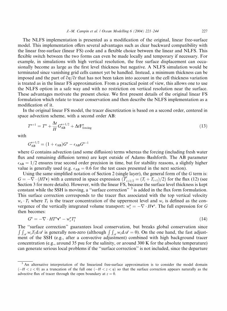
The NLFS implementation is presented as a modification of the original, linear free-surfacemodel. This implementation offers several advantages such as clear backward compatibility withthe linear free-surface (linear FS) code and a flexible choice between the linear and NLFS. Thisflexible switch between the two forms can even be made locally and temporary if necessary. Forexample, in simulations with high vertical resolution, the free surface displacement can occa-sionally become as large as the first level thickness but negative. A NLFS simulation would beterminated since vanishing grid cells cannot yet be handled. Instead, a minimum thickness can beimposed and the part of og=ot that has not been taken into account in the cell thickness variationis treated as in the linear FS approximation. From a practical point of view, this allows one to usethe NLFS option in a safe way and with no restriction on vertical resolution near the surface.These advantages motivate the present choice. We first present details of the original linear FSformulation which relate to tracer conservation and then describe the NLFS implementation as amodification of it.

In the original linear FS model, the tracer discretization is based on a second order, centered inspace advection scheme, with a second order AB:

3 A

ð�H <advec

T nþ1 ¼ T n þ DtH

Gnþ1=2AB þ DtFn

forcing ð13Þ

with

Gnþ1=2AB ¼ ð1 þ �ABÞGn � �ABGn�1

where G contains advection (and some diffusion) terms whereas the forcing (including fresh waterflux and remaining diffusion terms) are kept outside of Adams–Bashforth. The AB parameter�AB ¼ 1=2 ensures true second order precision in time, but for stability reasons, a slightly highervalue is generally used (e.g. �AB ¼ 0:6 for the test cases presented in the next section).

Using the same simplified notation of Section 2 (single layer), the general form of the G term is:G ¼ �r � ðHT vÞ with a centered in space expression ðT i

iþ1=2 ¼ ðTi þ Tiþ1Þ=2Þ for the flux (12) (seeSection 3 for more details). However, with the linear FS, because the surface level thickness is keptconstant while the SSH is moving, a ‘‘surface correction’’ 3 is added in the flux form formulation.This surface correction corresponds to the tracer flux associated with the top vertical velocityws � T1 where T1 is the tracer concentration of the uppermost level and ws is defined as the con-vergence of the vertically integrated volume transport: wn

s ¼ �r � Hvn. The full expression for Gthen becomes:

Gn ¼ �r � HT nvn � wnsT

n1 ð14Þ

The ‘‘surface correction’’ guarantees local conservation, but breaks global conservation sinceR RAwsT1dA is generally non-zero (although

R RAwsdA ¼ 0). On the one hand, the fast adjust-

ment of the SSH (e.g., after a convective adjustment) combined with high background tracerconcentration (e.g., around 35 psu for the salinity, or around 300 K for the absolute temperature)can generate serious local problems if the ‘‘surface correction’’ is not included, since the departure

n alternative interpretation of the linearized free-surface approximation is to consider the model domain

z < 0Þ as a truncation of the full one ð�H < z < gÞ so that the surface correction appears naturally as the

tive flux of tracer through the open boundary at z ¼ 0.


from the local conservation rule is precisely the correction term wsT1. On the other hand, themismatch in the global tracer content associated with this surface correction is generally small andgiven by:

4 N

VDT ¼ VTnþ1 �VT

n ¼ �DtZ Z

A

½ð1 þ �ABÞðwsT1Þn � �ABðwsT1Þn�1dA

where A, V are the ocean area and volume respectively and T is the global mean tracer con-centration.

For these reasons, most linear FS models that use a finite volume tracer discretization incor-porate such a surface correction (Marshall et al., 1997a; Roullet and Madec, 2000; Griffies et al.,2001).

In the implementation of the NLFS, the general method presented in Section 2 is adapted todeal with the original AB scheme. Using (4) and defining 4 wn

s ¼ �r � hnvn, Eq. (5) is equivalent to:

T nþ1 ¼ T n þ Dthnþ1

½�r � hnT nvn � wnsT

n1 þ PnðTrain � T1Þn ð15Þ

Eq. (15) is close to the original (linear FS) AB formulation ((13) and (14)) and allows us tointroduce the AB time stepping as follows:

T nþ1 ¼ T n þ Dthnþ1

½Gnþ1=2AB þ PnðTrain � T1Þn

and

Gn ¼ �r � hnT nvn � wnsT

n1 ð16Þ

with

Gnþ1=2AB ¼ ð1 þ �ABÞGn � �ABGn�1:

Using Eq. (4), this yields:

ðhnþ1T nþ1 � hnT nÞ=Dt ¼ �ð1 þ �ABÞr � ðhT vÞn þ �ABr � ðhT vÞn�1 þ ðPTrainÞn

� �AB½ðwsT1Þn � ðwsT1Þn�1 ð17Þ
This formulation has several advantages:
1. The same formulation can be used with both AB and forward two time-level (e.g., Lax–Wendr-off) time stepping: one recovers (15) by simply replacing Gnþ1=2

AB in (16) by Gn computed withLax–Wendroff fluxes (12). This returns the fully conservative scheme described in Section 2since (5) is equivalent to (17) with �AB ¼ 0. This formulation is also close enough to the originalformulation to involve only slight modifications in the code and to allow a switch back to thelinear FS option.

2. It is clear from (16) that the surface-level expansion/contraction term ðwsT1Þ inside the ‘‘Gn’’term ensures a precise local conservation, just as the surface correction does in the linear FScase. The reasons that motivate adding this surface level expansion term in Gn for the non-lin-

ote that ws is not the vertical velocity at the surface. This later quantity is given by: wz¼g ¼ ws þ vz¼g � rg.


ear case are similar to those given for the surface correction in the linear FS case. Since SSHcan exhibit fast variations, with the possibility of sign changes from one time step to the next,the amplitude of the local surface term (i.e. the last term in Eq. (17)) can be of the same orderas the surface correction ðwsT1Þn in the linear FS formulation. It therefore needs to be includedin the tracer Eqs. (16) and (17).

3. This formulation does not exactly conserve the global tracer content between time-steps, sincethe contribution of the surface level expansion term does not integrate to zero:

ðVT Þnþ1 � ðVT Þn ¼ ��AB

Z ZA

½ðwsT1Þn � ðwsT1Þn�1dA 6¼ 0:

However, this equation can be rearranged so that the global quantity

ðVT�Þnþ1 ¼

Z ZA

½ðhT Þnþ1 þ �ABDtðwsT1ÞndA ð18Þ

appears to be exactly conserved. Furthermore, this ‘‘modified’’ global tracer contentVT�

is a goodapproximation to the total tracer content VT since �ABDt

R RwsT1 dA is generally very small.

Therefore, the exact conservation of VT�

guarantees that the model tracer content cannot drift.4. For the purpose of checking tracer conservation, inaccuracy in local conservation is relatively

difficult to isolate whereas global conservation is easily diagnosed. Since our formulation ex-actly satisfies local conservation, we can evaluate the error in global conservation and provideestimates of the accuracy of the method. This is done in the next section.

5. Illustrative examples of property conservation

This section illustrates how the NLFS formulation previously described improves the conser-vation of various quantities, such as volume, temperature, salinity with time varying fresh waterforcing, and finally energy. Since NLFS effects are generally relatively small in the global oceanand difficult to isolate, here we consider only ideal tests with very simple geometry and concen-trate on free surface effects. A steady state problem like the Goldsbrough–Stommel circulationdescribed by Huang (1993) is not a selective test to address tracer conservation regarding the timestepping. For this reason, we prefer to include a strong time dependency in the test experimentpresented here. This is achieved by imposing a strong time dependent forcing or posing an initialadjustment problem.

The first test case is an ocean wind driven gyre circulation similar to the problem describedanalytically by Stommel (1948). The ocean depth is relatively shallow (H ¼ 400 m) to emphasizeNLFS effects which scale like g=H . There are four vertical levels each of 100 m. The domain is 59�wide in longitude and extends from the Equator to 59 �N on a spherical 1� 1� grid. The hori-zontal and vertical viscosity are 400 and 10�2 m2/s respectively, and the same values are used fordiffusivity. The time step is set to Dt ¼ 20 min. The initial state is at rest, horizontally uniform andthermally stratified h ¼ 20, 16, 12, 8 [�C]. Salinity is initially uniform (S0 ¼ 33 psu) and has noinfluence on density which is assumed to be only function of the potential temperature h:q ¼ q0ð1 � ahÞ with a ¼ 2 10�4 �C�1. A constant zonal wind stress is applied sx ¼ s0 sinðpu=LuÞwith s0 ¼ 0:1 Nm�2, u the latitude and Lu the domain latitudinal extension (59�).

In addition, a relatively strong fresh water forcing (E � P ) is added in the South-West cornerthat peaks at 1.5 m/day and linearly decreases toward the East and toward the North:


R0 ¼ ½16 � u � k � 0:1 m/day (k;u in� and R0 P 0), with a simple diurnal cycle: E � P ¼R0 sinð2pt=1dayÞ. It can be treated as a real fresh water flux (‘‘Real FW’’) ðþ ¼ out off the oceanÞwith the NLFS or converted to an equivalent salt flux (‘‘Salt Flx’’): FlxS ¼ Sc � ðE � P Þ=Dz1 (hereSc ¼ 35 psu) without direct effects on the SSH. In the case of the linear free surface, a ‘‘virtualfresh water’’ (‘‘Virtual FW’’) formulation can be defined, where E � P directly affects the SSH (asin real fresh water input) but needs to be converted to an equivalent salt flux to have an impact onthe salinity, since the thickness of the first layer is kept fixed (and consequently also the oceanvolume V). Table 1 provides a summary of these different options.

The fast variations of E � P allow one to check salt conservation when using various timestepping schemes; in the absence of thermal forcing, this simple case provides a good test of globaland local conservation of h during the initial adjustment of the SSH under the wind forcing. Notethat the dilution effect on salinity is present in all experiments (with real FW, virtual FW or saltFlx) but is decoupled from the dynamics since oq=oS ¼ 0. The fresh water impact on the dynamicsis limited to the direct effect on SSH and is only present when real FW or ‘‘virtual’’ FW is applied(Table 2, exp. 0, 5, 6, 9 and 10).

5.1. Volume conservation

The model exactly conserves volume in all cases, whether linear or NLFS, and whetherbackward ðb ¼ c ¼ 1Þ or Crank–Nickelson ðb ¼ c ¼ 1=2Þ time stepping of the free-surfaceequations.

With no real fresh water input, the average SSH remains equal to zero during a five dayssimulation with a deviation of less that 2 10�16 m, the level of computer precision. During thesame period, the SSH range (maximum–minimum) increases to 0.3 m. In the original formulation,volume conservation is less precise: after five days, the average SSH is )7 10�16 m (Fig. 1a) but itdrifts between )2 and )3 10�12 m over 10 years (Fig. 1b). With the new implementation, themean SSH remains zero with the same accuracy (few 10�16 m) over 10 years using equivalentoptions (backward time stepping and linear free-surface). The explicit integration of the conti-nuity equation (see details in Appendix A) prevents truncation and solver errors from accumu-lating. From here on we only consider the new formulation that exactly conserves the volume.

Several experiments of five day duration have been conducted with various combinations ofoptions, to test the robustness of the tracer conservation. The evolution of the global mean, thelowest and highest values of the SSH is plotted in Fig. 2a–c respectively, and correspond to fourexperiments (Table 2, exp. 3, 4, 5 and 6) that use different options: the free surface time stepping is

Table 1

Free surface formulation and fresh water treatment

Free surface equation Salinity equation Label

otg þr � ðH þ gÞv ¼ P otðhSÞ þ r � hSv ¼ 0 NL FS Real FW

otg þr � ðH þ gÞv ¼ 0 otðhSÞ þ r � hSv ¼ �P � Sc NL FS Salt flux

otg þr � Hv ¼ 0 otðHSÞ þ r � HSv ¼ �P � Sc Lin FS Salt fux

otg þr � Hv ¼ P otðHSÞ þ r � HSv ¼ �P � S Lin FS Virtual FW

Table 2

Accuracy of the global conservation of heat and salt using various combination of options relative to the free surface

treatment and the tracer advection scheme.

Experiment number and options Global mean deviation

N Linear/Non Flux FS stepping Advection Dh (�C) DS (psu)

0 Lin FS Virtual FW Back LW 5 10�7 7 10�6

1 Lin FS Salt Flx Back LW 2 10�7 2 10�7

2 Lin FS Salt Flx CrNi LW 2 10�7 4 10�7

3 NL FS Salt Flx Back LW 0 1 10�12

4 NL FS Salt Flx CrNi LW 0 1 10�12

5 NL FS Real FW Back LW 0 2 10�12

6 NL FS Real FW CrNi LW 0 2 10�12

7 Lin FS Salt Flx Back AB 2 10�7 2 10�7

8 NL FS Salt Flx Back AB 3 10�9 6 10�9

9 NL FS Real FW Back AB 2 10�8 9 10�8

10 NL FS Real FW CrNi AB 3 10�8 1 10�7


either implicit (exp. 3 and 5) or Crank–Nickelson (exp. 4 and 6); the fresh water forcing is eitherreal FW (exp. 5 and 6) or converted to salt flux (exp. 3 and 4).

In our experiments, the dynamical behavior of the SSH is not sensitive to the tracer advectionscheme or whether the free surface is linear or non-linear and so only four experiments among the11 listed in Table 2 are shown in Fig. 2, all 4 using NLFS with Lax–Wendroff advection scheme.

The global mean SSH exactly match the integrated fresh water input or remains flat when saltflux is used. Under wind stress forcing, the SSH slowly builds up low and high large scale surfacepressure patterns (Fig. b, c, exp. 3 and 4). Superimposed on this slow tendency, strong, local realfresh water forcing (exp. 5 and 6) generates local excursions of SSH that are of the same mag-nitude (around 0.3 m) as the wind driven adjustment after five days. Using a Crank–Nickelsontime stepping produces slightly higher SSH standard deviation (in space) and larger SSH ex-cursions than the implicit scheme. This is related to the damping properties of the backward timestepping procedure and will be discussed in sub-section (c).

5.2. Tracer conservation

Tracer conservation is expressed differently according to the boundary condition used forE � P : with real fresh water input, the ocean volume V changes but the total salt content VSremains constant. The total heat content can change because the water input enters or leaves thesurface with temperature hrain that is usually equal to the local surface temperature. Here, forsimplicity, we set hrain ¼ 14 �C which also corresponds to the global mean initial temperatureensuring that global mean temperature is conserved. When salt flux or ‘‘virtual fresh water’’ fluxare used, the volume is constant and the global mean temperature is also unchanged. In this case,the global mean salinity follows the time and space integrated salt flux:

SFxSðtÞ ¼ S0 þScV

Z t

0

Z ZA

ðE�

� PÞdA�

dt

0 1 2 3 4 5 6 7 8 9 10–3.5

–3

–2.5

–2

–1.5

–1

–0.5

0

0.5x 10–12

Time [yr]

OriginalNew

0 0.5 1 1.5 2 2.5 3 3.5 4 4.5 5–8

–6

–4

–2

0

2x 10–16

Time [days](a)

(b)

OriginalNew

Fig. 1. Evolution of the global mean SSH (m) with the original model (back line) and the new formulation (gray line)

which includes an explicit integration of the continuity equation (see Appendix A). The linear free-surface with

backward time stepping is used without fresh water input. Fig. 1a (top) corresponds to the first five days of the sim-

ulation that has been extended up to 10 years (Fig. 1b, bottom).


The degree of conservation is expressed in both cases in terms of global mean temperature de-viation: Dh ¼ h � h0 and equivalent mean salinity deviation: DS ¼ SV=V0 � Sref correspondingto the global salt content minus the theoretical value Sref ¼ S0 or Sref ¼ SFxSðtÞ.

The range of variations (maximum DT minus minimum DT ) of temperature and salinity aregathered in Table 2. The computer precision is such that the accuracy of integrated quantities,for example the mean salinity, cannot be better than 10�12.

0 0.5 1 1.5 2 2.5 3 3.5 4 4.5 5–0.3

–0.25

–0.2

–0.15

–0.1

–0.05

0

0.05

Time [days]

exp.6exp.5exp.4exp.3

0 0.5 1 1.5 2 2.5 3 3.5 4 4.5 50

0.1

0.2

0.3

0.4

0.5

Time [days]

exp.6exp.5exp.4exp.3

0 0.5 1 1.5 2 2.5 3 3.5 4 4.5 5–8

–6

–4

–2

0

2x 10–3

Time [days]

Avr SSH [m]

Min SSH [m]

Max SSH [m]

(a)

(b)

(c)

Fig. 2. Evolution of mean (Fig. 2a, top), minimum (Fig. 2b, middle) and maximum (Fig. 2c, lower) of the SSH [m] over

the full domain. Results of four experiments are plotted: exp. 3, continuous black line; exp. 4, dash black line; exp. 5,

continuous gray line; exp. 6, dash gray line.



The first set of experiments (exp. 0–6) uses the forward Lax–Wendroff scheme and confirms theexact conservation of heat and salt of the NLFS implementation, with or without real fresh waterinput. By contrast, the LinFS formulation exhibits small deviations (�10�7) for both temperatureand salinity (Fig. 3a,b). These are associated with the integrated ‘‘surface correction’’ term �wsTs(see Section 4). The area integrated surface correction is relatively small but can accumulate intime and may produce a significant drift, as in experiment 0 (Fig. 3c) in which the mean salinitydecreases by 7 10 �6 psu in five days, corresponding to 0.5 10�3 psu/yr.

The reason for the large drift in exp.0 is the presence of the strong diurnal cycle of E � P thatdirectly affects the SSH (‘‘virtual fresh water’’ flux), whereas the other LinFS experiments use onlysalt flux. During the first half of the day, E � P > 0 is applied to the SSH and adjustment of thebarotropic flow results in convergent motion, positive ws and a large negative surface correction�wsS1, since S1 is locally larger than the mean salinity due to E � P effects. When E � P reversesduring the second half of the day, the surface correction becomes positive but smaller than theamplitude of the negative peak, since advection and diffusion processes have already eroded thesalinity maxima. While ws is globally balanced at each time step and locally balanced over a oneday period, the two half-day contributions of the surface correction term do not balanceð�wsS1Þ� þ ð�wsS1Þþ < 0, and the net integral effect over one diurnal cycle is clearly negative,resulting in a negative drift of the mean salinity (Fig. 3c).

The second set of experiments (exp. 7, 8, 9 and 10) uses the three time-level Adams–Bashforthadvection scheme, and yields non-exact global conservation (Table 2). The conservation is betterwith the NLFS formulation than with the linear free surface, especially when the comparison isrestricted to identical E � P forcing experiments, (exp. 8 versus 7). Note that exp. 9 can also becompared to exp. 0 since this later experiment has been repeated using the AB scheme and yieldsthe same salinity and temperature drift as exp. 0.

The NLFS conservation is not only more accurate than the linear one, but also improvedqualitatively: the tracer deviation does not drift with NLFS but tends to remain around the zeroline. This is specially true in experiment 9 (or 10) which incorporates real fresh water input andexhibits relatively high temperature and salinity deviations compared to other NLFS simulations(Table 2). However the deviation always returns to almost zero at the end of each day (Fig. 3a,b).This is in agreement with the ‘‘error cancellation’’ idea developed in Section 4, which prevents anysignificant drift to develop. This can be differently expressed as the exact conservation of the‘‘modified’’ global mean temperature h

�and salinity S

�defined according to Eq. (18). In order to

precisely check this property, the surface integral of the surface level expansion term: SeðT Þ ¼Dt=V

R RAðwsT1ÞdA is computed for temperature ðT ¼ hÞ and salinity ðT ¼ SÞ and the modified

global mean tracer concentration derived thus, T� ¼ T þ �ABSeðT Þ. Fig. 4 plots the evolution of

the temperature deviation Dh, the surface level expansion term SeðhÞ and the modified meantemperature deviation Dh� (Fig. 4a) for exp. 8 (equivalent salt flux forcing), and similarly for thesalinity DS, SeðSÞ and DS� (Fig. 4b) for exp. 10 (real FW forcing). The SSH variations are only dueto wind forcing in exp. 8, and are much weaker than in exp. 10 in which real fresh water is added.Therefore the magnitude of the surface level expansion term is also much weaker in exp. 8 (�10�9)than in exp. 10 (�10�7) and has no diurnal cycle. Despite those differences, in both experimentsthe global mean deviation is exactly canceled when the surface level expansion term is added withthe Adams–Bashforth factor �AB, resulting in perfect conservation of the modified global meantemperature in exp. 8 and salinity in exp. 10. The agreement is perfect in all the Adams–Bashforth

0 0.5 1 1.5 2 2.5 3 3.5 4 4.5 5–20

–15

–10

–5

0

5x 10–8

Time [days]

∆ θ [oC]

(a)

(b)

(c)

exp.6exp.2exp.9exp.8exp.7

0 0.5 1 1.5 2 2.5 3 3.5 4 4.5 5–2

–1.5

–1

–0.5

0

0.5

1

1.5

2x 10–7

Time [days]

∆ S [psu]

exp.6exp.2exp.9exp.8exp.7

0 0.5 1 1.5 2 2.5 3 3.5 4 4.5 5–7

–6

–5

–4

–3

–2

–1

0

x 10–6

Time [days]

∆ S [psu]

exp.2exp.0

Fig. 3. Evolution of global mean tracer deviation for potential temperature Dh (Fig. 3a, top) and salinity DS (Fig. 3b

and c) corresponding to six experiments (see Table 2).


0 0.5 1 1.5 2 2.5 3 3.5 4 4.5 5–3

–2

–1

0

1

2

3

4x 10–9

Time [days]

exp.8

(a)

(b)

∆ θ Se(θ) ∆ θ*

0 0.5 1 1.5 2 2.5 3 3.5 4 4.5 5–1

–0.5

0

0.5

1

1.5x 10–7

Time [days]

exp.10

∆ S Se(S) ∆ S*

Fig. 4. Conservation of global mean tracer content with NLFS and AB time stepping: the evolution of the global mean

deviation DT (continuous line), the surface level expansion term SeðT Þ (dotted line) and the modified global mean tracer

T � (dash line) are plotted for (a) potential temperature in exp. 8 with salt flux and FS backward time stepping (top); and

(b) salinity in exp. 10 with real fresh water and FS Crank–Nickelson time stepping (bottom).


NLFS experiments (7, 8, 9 and 10), for both temperature and salinity, within 2 10�12 (�C or psurespectively).

From a practical point of view, the exact conservation of T�

implies that the global mean tracerconcentration is conserved, whatever the length of simulation, to within a factor �ABSeðT Þ, that issmall enough for all practical use of the model. Here in exp. 10, this terms remains smaller than10�7 psu, and given the strong and rapidly varying fresh water forcing, this is probably close to anupper bound.


5.3. Energy conservation

Energy budget analysis can be quiet difficult to carry out in a realistic global ocean model:energy is involved in all ocean processes and altered by numerical details. Therefore, for thepurpose of checking the energy conservation of the barotropic dynamics, the model is set up in avery simple configuration. With no forcing and initially at rest, the homogeneous, one layer oceanmodel adjusts to an initial bump in SSH centered on the equator. The shape of the initial bump isgiven by gt¼0 ¼ Dh0 � ½1 � cosðp � ð1 � rÞÞ=2 with r the normalized radial distance from the center

of the bump: r ¼ minð1;ffiffiffiffiffiffiffiffiffiffiffiffiffiffix2 þ y2

p=RbumpÞ; the radius of the bump is Rbump ¼ 30� and the maxi-

mum height at the center is Dh0 ¼ 100 m. The spherical grid resolution is 2.8125� 2.8125� andthe ocean depth is uniform (H ¼ 1 km) and without continents. For simplicity, only non-rotatingcases are considered here and the Coriolis parameter is set to zero. 5 The time step Dt ¼ 450 s issmall enough to resolve external gravity waves at the equator. The small grid spacing near thepoles does not limit the time step since both backward or Crank–Nickelson time stepping areunconditionally stable. This is an advantage compared to explicit methods that require a verysmall time step to satisfy the stability criteria near the poles.

Five different simulations illustrate the evolution of model energy (Figs. 5 and 6). The firstexperiment (‘‘Back_Lin’’) uses the free surface backward time stepping in a pure linear case, i.e,linear free surface with no momentum advection. The remaining four use Crank–Nickelson timestepping, either with the same linear formulation (standard experiment, ‘‘CrNi Lin’’), adding onlymomentum advection (‘‘CN Ln + Adv’’), adding only NLFS effects (‘‘CN NonLin’’) or addingboth (‘‘CN NL + Adv’’). For momentum advection, the Adams–Bashforth time stepping is usedand for this test �AB is set to 1/2.

The adjustment problem is symmetric with respect to the center of the initial bump so thattaking a section across this center provides a good view of a global field. The SSH along theequator is represented in Fig. 5 at time 0, 1.5, 3, 4.5 and 4.72 days of simulation, in the five ex-periments. In addition, the evolution of global quantities such as the maximum range of SSH(highest point minus lowest point values), the volume mean KE and PE and the mean total energy(PE + KE) is represented in Fig. 6. The volume mean PE and KE are expressed both in m2/s2 andcomputed as follows:

5 Th

analyt

discre

conser

free-su

PE ¼ 1

V

Z ZA

1=2gg2dA and KE ¼ 1

V

Z ZA

h1=2ðu2 þ v2ÞdA

When the linear free surface approximation is made, the time dependent ocean thickness h is keptconstant and set equal to H in the KE expression.

The standard experiment (‘‘CrNi_Lin’’) is free of non-linear effects and therefore easier tointerpret. The initial SSH anomaly generates gravity waves that propagate in a radial direction

e simplicity of the non-rotating, purely linear test (detailed in the body of the text) allows one to find an

ical solution using spherical harmonics to verify model results. This also avoids complications concerning the

tization of the Coriolis term on a C-grid, a delicate issue which can have significant impact on energy

vation. Such aspects, although important, go beyond the scope of this paper where we prefer to concentrate on

rface effects only.

–150 –100 –50 0 50 100 150

0

50

100 time= 0.00 d

time= 1.50 d

time= 3.00 d

time= 4.50 d

time= 4.71 d

Back Lin CrNi Lin CN Ln+AdvCN NonLinCN NL+Adv

–150 –100 –50 0 50 100 150–10

0

10

20

–150 –100 –50 0 50 100 150–20

–10

0

10

–150 –100 –50 0 50 100 150–30

–20

–10

0

10

–150 –100 –50 0 50 100 150–100

–50

0

Fig. 5. SSH [m] along the equator corresponding to (from top to bottom) time 0.0, 1.5, 3.0, 4.5 and 4.71 days. Results

from five experiments (Back_lin, CrNi lin, CN Ln + Adv, CN NonLin and CN NL + Adv, see Section 5.3) are plotted.


from the source (Long 0.E) and converge to the symmetric point relative to the sphere center, at180.E on the equator, before coming back to the source point at time t ¼ Tcycle ’ 4:71 days. Tcycle isdefined as the time of the first maximum and minimum of, respectively, the mean potential and

0 0.5 1 1.5 2 2.5 3 3.5 4 4.5 5

0

50

100

150

Time [days]

(a) Max_min SSH

Back Lin CrNi Lin CN Ln+AdvCN NonLinCN NL+Adv

0 0.5 1 1.5 2 2.5 3 3.5 4 4.5 5

0

0.2

0.4

0.6

0.8

Time [days]

(b) Mean KE

0 0.5 1 1.5 2 2.5 3 3.5 4 4.5 5

0

0.2

0.4

0.6

0.8

Time [days]

(c) PE(eta)

0 0.5 1 1.5 2 2.5 3 3.5 4 4.5 5–0.4

–0.3

–0.2

–0.1

0

0.1

Time [days]

(d) PE+KE

Fig. 6. Evolution of global quantities for five experiments (Back lin, CrNi lin, CN Ln + Adv, CN NonLin and

CN NL + Adv, see Section 5.3): (a) SSH range (maximum–minimum) [m]; (b) Mean KE [m2/s2]; (c) Mean PE [m2/s2];

(d) Total energy PE + KE deviation from the initial value (0.55375) [m2/s2]. The dash line at t ¼ 4:71d corresponds

to the minimum of KE and maximum of PE.



KE, and can be considered as the time period required for the energy to travel around the sphere.Tcycle is slightly longer than the period T0 of non-dispersive plane waves in a cyclic channel:T0 ¼ 2pRE=

ffiffiffiffiffiffiffigH

p¼ 4:68d ¼ 112:25h with RE ¼ 6370 km the Earth radius. This is due to the dis-

persive nature of gravity waves on the sphere (Panchev, 1985, p. 179) and also explains the reversesign of the SSH anomaly after 1 cycle ðt ¼ TcycleÞ. The numerical dispersion that mainly affectspoorly resolved wave lengths and frequencies is relatively small here, since the shape of the bumpis well preserved after one cycle in the pure linear case (Fig. 5d, CrNi_Lin).

Adding momentum advection or relaxing the Linear FS approximation does not change thegeneral behavior of wave propagation but increases the dispersion and results in significant phasedifferences; this appears clearly on Fig. 5 after 4.5 days of integration. On the contrary, use ofbackward time stepping ðexp ¼ Back LinÞ has only minor phase effects but strongly reduces theamplitude of the SSH anomaly, up to 50% of its initial value after one cycle.

Use of backward time stepping is the largest source of differences in energy evolution (Fig. 6b–d) and maximum range of SSH (Fig. 6a). The damping of fast modes with backward time steppingis responsible for a large decrease in the total energy (more that 50% after four days) (Fig. 6d) anda reduction of the wave amplitude by roughly the same factor. By contrast, non-linear effectson the phase and the shape of the SSH anomalies also modify the evolution of the SSH rangebut have only a weak influence on the energetics of the system.

The conservation of the total energy is exact in the standard case (no advection of momentumand linear free surface). The departure from the initial value is less that 10�13 m2/s2 during thewhole simulation (five days), at the level of machine precision. Without momentum advection, theNLFS formulation does not conserve the total energy, as shown on Fig. 6d. The departure fromthe initial value is 0.02 m2/s2 (<5% of the total) after five days. This property has been notedbefore (see e.g., Roullet and Madec, 2000; Griffies et al., 2001) and is related to the coupling ofmomentum advection and free surface displacement in the KE budget, which can no longer beconsidered separately, in contrast to the linear FS case. This motivates the inclusion of mo-mentum advection terms in the NLFS experiment CN NL + Adv and, for comparison, the linearFS experiment CN Ln + Adv.

Energy conservation is less simple in the presence of momentum advection terms than tracerconservation. Given the objective of this paper, our priority is tracer conservation. Nevertheless,use of the NLFS significantly improves energy conservation; the total energy drifts by less than1.9 10�3 m2/s2 in the NLFS case CN NL + Adv but exceeds 0.02 m2/s2 in the linear FS exper-iment CN Ln + Adv.

The poor energy conservation of the linear FS case is related to the ‘‘surface correction’’ term,�ws:v in the momentum equation that is designed to conserve locally the momentum, whereasglobal conservation of energy required only half of it. In the NLFS case, a significant improve-ment in energy evolution can be expected by simply changing the definition of the cell thickness tohi, h

jat U,V points; as mentioned by Roullet and Madec (2000), in order to conserve energy an

area weighted mean value between the two neighbors must be used hi ¼ ðAihi þAiþ1hiþ1Þ=2A

i

instead of the minimum of the two, to ensure that the time variation of hi

corresponds to wsiDt.

With momentum advection and including those two modifications (half of the surface cor-

rection in CN Ln + Adv and modified hi, h

jin CN NL + Adv, hereafter referenced as

CN NL� + Adv, the energy conservation is still not exact, due to the use of Adams–Bashforth formomentum advection. However, the departure from the initial PE remains very small during the


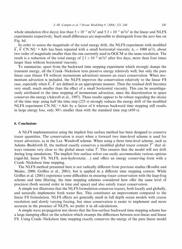
whole simulation (five days); less than 5 10�5 m2/s2 and 5.3 10�5 m2/s2 in the linear and NLFSexperiments respectively. Such small differences are impossible to distinguish from the zero line onFig. 6d.

In order to assess the magnitude of the total energy drift, the NLFS experiment with modifiedhi, h

jCN NL� + Adv has been repeated with a small horizontal viscosity Ah ¼ 1000 m2/s, about

two order of magnitude smaller than the one currently used in OGCM at the same resolution. Theresult is a reduction of the total energy of 2.1 10�4 m2/s2 after five days, more than four timeslarger than without horizontal viscosity.

To summarize, apart from the backward time stepping experiment which strongly damps thetransient energy, all the Crank–Nickelson tests preserve energy relatively well, but only the purelinear case (linear FS without momentum advection) ensures an exact conservation. When mo-mentum advection is included, the NLFS improves the conservation relatively to the linear FScase, especially when h

i, h

jare defined in an appropriate manner. Then the residual drift becomes

very small, much smaller than the effect of a small horizontal viscosity. This can be unambigu-ously attributed to the time stepping of momentum advection, since the discretization in spaceconserves the energy (Adcroft et al., 1997). These results appear to be robust regarding the choiceof the time step: using half the time step (225 s) strongly reduces the energy drift of the modifiedNLFS experiment CN NL� + Adv by a factor of 6 whereas backward time stepping still resultsin large energy loss, only 30% smaller than with the standard time step (450 s).

6. Conclusions

A NLFS implementation using the implicit free surface method has been designed to conservetracer quantities. The conservation is exact when a forward two time-level scheme is used fortracer advection, as in the Lax–Wendroff scheme. When using a three time-level scheme, such asAdams–Bashforth II, the method exactly conserves a modified global tracer content T

�that al-

ways remains very close to the global mean value T . This ensures that the model will not driftduring long simulations. The implicit free surface solver can easily accommodate various options(rigid-lid, linear FS, NLFS, non-hydrostatic. . .) and offers an energy conserving form with aCrank–Nickelson time stepping.

The NLFS method presented here is not radically different from previous studies (Roullet andMadec, 2000; Griffies et al., 2001), but is applied in a different time stepping context. WhileGriffies et al. (2001) experience some difficulties in ensuring tracer conservation with the leap-frogscheme and time filtering, the time stepping schemes considered here offer the same level ofprecision (both second order in time and space) and also satisfy tracer conservation.

A simple test illustrates that the NLFS formulation conserves tracers, both locally and globally,and naturally implements fresh water flux. This constitutes an improvement compared to thelinear FS formulation. NLFS effects are generally small in full depth ocean models with coarseresolution and slowly varying forcing, but since conservation is easier to implement and moreaccurate in the presence of NLFS, we prefer it in all calculations.

A simple wave propagation test shows that the free-surface backward time stepping scheme hasa large damping effect on the solution which swamps the differences between non-linear and linearFS. Using Crank–Nickelson time stepping exactly conserves the energy of the pure linear model


(linear FS without momentum advection) and allows us to identify NLFS effects on the phasepropagation of gravity waves. When momentum advection is included, energy conservation isbetter with the NLFS formulation than with the linear FS form, and can be further improved witha small modification of the grid interface thickness. However this modification does not induceany noticeable effects on wave features.

Emphasis is often put on the role of space discretization in energy budget consistency(Dukowicz and Smith, 1994; Adcroft et al., 1997; Roullet and Madec, 2000; Griffies et al., 2001)but rarely on time stepping effects. Despite this, very few numerical simulations actually ex-hibit accurate energy conservation. The simple barotropic adjustment test presented here indi-cates that time stepping effects can be much larger than discretization in space. Therefore, wesuggest that any energy conservation analysis should consider both the time and space discreti-zation.

Backward time stepping is commonly used for the free surface equation (Dukowicz and Smith,1994; Wolff et al., 1997; Marshall et al., 1997b) and results in energy loss (e.g., the simplebarotropic adjustment test, Section 5.3). This requires some comments:

(a) There is no doubt that the test (5.c) presented here is over simplified. The magnitude of energyloss is probably extreme, but is indicative of behavior in more realistic ocean models that usethe same free-surface time stepping. Note that other time stepping methods such as the splitexplicit FS also damp the energy of the external mode since time averaging is used with themethods and is not supposed to be energy conserving.

(b) According to Arakawa (1966)––and often quoted––energy conservation offers a limited ad-vantage, mainly in terms of stability of the momentum advection discretization. To accuratelyrepresent the evolution of the distribution of energy as a function of scale, conservation ofboth energy and enstrophy are required. However, such a scheme (Arakawa, 1966) has notyet been successfully implemented in a z-coordinate OGCM, probably because it is not easilydone. Regarding the stability objective, alternative methods exist to ensure a stable discreti-zation of the momentum advection terms (see for e.g., Tartinville et al., 1998), as for instanceenergy decreasing schemes known as Total Variance Diminishing schemes.

(c) In coarse resolution, non-eddy resolving models, the KE that the model contains is not rep-resentative of the real ocean KE which is mainly contained in the eddy field (Stammer andB€ooning, 1985). In this case energy conservation is perhaps not a major concern. However,when eddying motions are permitted, low energy dissipation numerics are required in orderto carry out accurate simulations of ocean dynamics. For this purpose, a relatively accurateenergy conservation is sufficient and does not need to be exact. This justifies some recentdevelopments which are presented as energy conserving (Adcroft et al., 1997; Roullet andMadec, 2000; Griffies et al., 2001), even if conservation is not exact because of the free-sur-face time stepping.

Depending on the particular application, the damping of the fast external gravity waves can bejustified, providing it does not alter the essential features of interest. This is what happens whenthe backward time stepping and more generally a non-energy conserving free-surface method isused. In other applications, such as in the simple barotropic adjustment problem, an energyconserving scheme for the external mode, such as the Crank–Nickelson time stepping, is crucial.


The NLFS implementation in the MITgcm uses the implicit free surface method and allows us toselect the external mode time stepping appropriate for each modeling study.

Acknowledgements

We wish to thank Stephen Griffies and an anonymous reviewer for constructive comments thatgreatly improved the manuscript. This work was supported by the ECCO project (Estimating theCirculation and Climate of the Ocean) and the MIT Climate Modeling Initiative.

Appendix A

The explicit integration of the column integrated continuity Eq. (4) was not present in theoriginal model (Marshall et al., 1997a) and has been added for the purpose of the NLFS (seeSection 2). However, for the linearized formulation, we find it useful to retain the integration ofthe linearized Eq. (4):

ðhnþ1 � hnÞ=Dt ¼ �r � Hvn þ Pn

in order to provide the SSH ðhnþ1 � HÞ on the right hand side of the linearized Eq. (10):

gnþ1 � bcDt2r � Hgrgnþ1 ¼ ðhnþ1 � HÞ þ bDtP nþ1 � bDtr � Hv� ðA:1Þ
This is slightly different from the original, backward ðb ¼ c ¼ 1Þ, linear free-surface formulationwhere gn was used in place of ðhnþ1 � HÞ in (A.1). The advantage of keeping an explicit integrationof the continuity Eq. (4) is that it ensures an exact volume conservation (see 5.a for a quantitativeestimation).
References

Adcroft, A., Campin, J.-M., Heimbach, P., Hill, C., Marshall, J., 2002. MITgcm release 1 manual. Technical report,

Massachusetts Institute of Technology, Cambridge, MA, 346 pp. http://mitgcm.org/sealion.

Adcroft, A., Hill, C., Marshall, J., 1997. Representation of topography by shaved cells in a height coordinate ocean

model. Monthly Weather Review 125, 2293–2315.

Arakawa, A., 1966. Computational design for long-term numerical integration of the equations of fluid motion: Two-

dimensional incompressible flow. Part I. Journal of Computational Physics 1, 119–143.

Dukowicz, J.K., Smith, R.D., 1994. Implicit free-surface method for the Bryan-Cox-Semtner ocean model. Journal of

Geophysical Research 99, 7991–8014.

Griffies, S., B€ooning, C., Bryan, F., Chassignet, E., Gerdes, R., Hasumi, H., Hirst, A., Treguier, A.-M., Webb, D., 2000.

Developments in ocean climate modelling. Ocean Modelling 2, 123–192.

Griffies, S., Pacanowski, R., Schmidt, M., Balaji, V., 2001. Tracer conservation with an explicit free surface method for

z-coordinate ocean models. Monthly Weather Review 129, 1081–1098.

Huang, R.X., 1993. Real freshwater flux as a natural boundary condition for the salinity balance and thermohaline

circulation forced by evaporation and precipitation. Journal of Physical Oceanography 23, 2428–2446.

Killworth, P.D., Stainforth, D., Webb, D.J., Paterson, S.M., 1991. The development of a free surface Bryan-Cox-

Semtner model. Journal of Physical Oceanography 21, 1333–1348.

Marshall, J., Adcroft, A., Hill, C., Perelman, L., Heisey, C., 1997a. A finite-volume, incompressible Navier Stokes

model for studies of the ocean on parallel computers. Journal of Geophysical Research 102, 5753–5766.

http://mitgcm.org/sealion


Marshall, J., Hill, C., Perelman, L., Adcroft, A., 1997b. Hydrostatic, quasi-hydrostatic, and nonhydrostatic ocean

modeling. Journal of Geophysical Research 102, 5733–5752.

Panchev, S., 1985. Dynamic Meteorology. Kluwer Academic, Dordrecht, Holland, p. 360.

Roullet, G., Madec, G., 2000. Salt conservation, free surface, and varying levels: a new formulation for ocean general

circulation models. Journal of Geophysical Research 105, 23927–23942.

Stammer, D., B€ooning, C.W., 1985. Generation and distribution of mesoscale eddies in the North Atlantic Ocean. In:

Krauss, W. (Ed.), The Warmwatersphere of the North Atlantic Ocean. Gedr€uuder Borntraeger, Berlin, Germany,

pp. 159–193.

Stommel, H., 1948. The western intensification of wind-driven ocean currents. Transactions of the American

Geophysical Union 29, 206.

Tartinville, B., Deleersnijder, E., Lazure, P., Proctor, R., Ruddick, K.G., Uittenbogaard, R.E., 1998. A coastal ocean

model intercomparison study for a three-dimensional idealised test case. Applied Mathematical Modelling 22, 165–

182.

Wolff, J.O., Maier-Reimer, E., Legutke, S., 1997. The Hamburg Ocean Primitive Equation model HOPE. Technical

Report 13, Max-Planck-Institut f€uur Meteorologie, DKRZ, Hamburg, Germany, 98 pp.

conservation of properties in a free-surface modelaja/papers/campin_et_al_om_2004.pdf ·...

Documents