Consciousness-related interactions in a double-slit optical system

Gabriel Guerrer∗

Instituto de Psicologia da Universidade de Sao Paulo, SP, Brasil

February 1, 2018

Abstract

Motivated by a series of reported experiments and their controversial results, the presentwork investigated if volunteers could causally affect an optical double-slit system by mentalefforts alone. The participants’ task in an experimental session alternated between intendingthe increase of the (real-time feedback-informed) amount of light diffracted through a specificsingle slit versus relaxing their intentional effort. In total, 240 sessions contributed by 171volunteers were recorded. The first 160 sessions were collected in an exploratory mode; thosedata revealed statistically significant differences between the intention and relax conditions.The analysis method and variables of interest derived from the exploratory sessions werethen pre-registered for the subsequent 80 formal sessions. The formal experiments, basedon a directional hypothesis, were not statistically significant. A post hoc analysis based ona bi-directional hypothesis, and applied to the same data, resulted in a 2.75 sigma outcome(p = 6.02 × 10−3; es = 0.31 ± 0.22 95% CI). All exploratory and formal studies combinedwithin the bi-directional analysis resulted in a 4.73 sigma effect (p = 2.28 × 10−6; es =0.35 ± 0.15 95% CI). Directional and bi-directional analyses applied to an equal numberof control sessions, all conducted without observers present, resulted in uniformly non-significant outcomes. Analysis of environmental factors did not reveal any artifactual sourcesthat might have produced the significant bi-directional effect. These results provide partialsupport for the previously claimed existence of anomalous interactions between consciousagents and a physical system.

1 Introduction

One of the hardest problems still unsolved by modern science concerns the nature of conscious-ness and its relationship to matter [1]. The millennial old debate, currently addressed by thephilosophy of mind, proceeds by asking if there are more fundamental aspects to reality, whatare their properties, and how do they interact.

The first time physicists seriously considered the possibility of a role for consciousness withintheir discipline coincided with the development of quantum mechanics in the 20th century.In particular, the question of how the superposition state is reduced to a definite observedstate, known as the quantum measurement problem, led some scientists [2–4] to associate suchabrupt transitions with an increase in subjective knowledge. According to that interpretation,the conscious agent played an essential role in promoting the state reduction when gaininginformation by interacting with the experimental apparatus.

The question evolved into a controversial philosophical and theoretical debate [5–11] wherethe majority today denies the necessity of any “extra-physical” consciousness ingredient in quan-tum physics [12]. Data in support of the leading view is found in “which-path” experiments,reported and discussed by [13]. Those experiments reveal that a sufficient condition for a super-position state collapse is the availability of ”which-path” information, even when theoretically

∗guerrer@usp.br / gabrielguerrer@gmail.com

1

obtainable but not effectively measured. The examples provided in [13] lead to the conclusionthat information reaching human consciousness is not a mandatory step for state reduction.

Although a strong role for human consciousness in the quantum measurement problem maybe ruled out, a weaker but theoretically highly significant role can be investigated; if the rightconditions are met, can consciousness influence the collapse of the superposition state? Or,more generally, is there any sort of interaction between consciousness-related mental states andquantum systems?

Experimental efforts to address the above questions date back to the 1970’s with the useof random number generators. These devices use quantum effects such as radioactive decayand tunneling to produce truly random binary numbers. In those studies, participants tried todirectionally bias the 0 or 1 outcomes from 50/50 chance through their mental intention, usuallybeing informed in real time about the measured values. Two major meta-analyses [14,15] havereported statistical evidence for the anomalous correlation between conscious intention and theoutput of random number generators. The results revealed a goal-oriented characteristic, wherethe increase in 0 or 1 coincides with the participant’s intended aim. Although significant, [15]concluded that the effect could be more simply explained as an artifact attributable to non-significant unpublished studies. That interpretation was argued as insufficient by the authorsof the first meta-analysis [16].

A double-slit system as a target in a similar experimental protocol was first used by [17].In the standard double-slit system if partial which-path information is obtained by any means,one expects a reduction in the interference component [18]. That study investigated the fringevisibility (a measure of the interference component) variation according to the participant’sintention. Two experiments were presented, one supporting the interaction hypothesis and theother conforming to chance expectations.

Of particular interest to the present work are the double-slit experiment series [19–22] pre-sented by Dean Radin and his collaborators. Those results are remarkable in the sense thatmany of the pre-planned experiments resulted in statistically significant evidence supporting theinvestigated interaction. Their findings, across the work series, claim that the observed effects:a) globally support the psychophysical interaction hypothesis, i.e. the causal effect of the partic-ipant’s intention in the optical system (the nomenclature of “mind-matter interaction” is alsoused); b) cannot be explained as procedural or analytical artifacts, as the control sessions (with-out participants present) resulted in no significant differences between the intention-present andintention-absent epochs; c) are stronger for participants with contemplative practices training,e.g. meditation; d) show a positive correlation to the participant’s score obtained in an ab-sorption questionnaire [23], which measures the degree of immersion that one can reach whenperforming a task; e) show a positive correlation to α-band desynchronization, a marker of ashift in attention as measured by an electroencephalogram; f) are retro-causal, i.e. obtainableeven when the participant views previously recorded data that was not observed by any par-ticipant or the experimenter prior to the session; g) do not depend on distance, occurring evenwhen the participant tries to exert influence on a distant optical system while receiving thefeedback information about the state of the interference pattern streamed over the internet. Asa result, the effect sizes obtained do not appear to decline with distance.

Inspired by Radin et al’s challenges to the present scientific world view, the current ex-periment tried to replicate their first four findings using a similar protocol and a modifiedsetup/analysis as described below.

2

2 Methods

2.1 Equipment

A semiconductor laser diode L (DL-3148-023, single mode λ = 635 nm, transverse magneticpolarization; Sanyo) is powered through a feedback driver circuit to maintain a constant 3 mWlight output power. To minimize temperature fluctuations, the laser diode is mounted on ametal structure covered with styrofoam. No lenses or neutral density filters are employed.

As depicted in Fig. (1), the laser light passes through two slits DS etched in a metal foil(10 µm width each, centrally-separated by 200 µm; Lenox Laser). The resulting interferencepattern is recorded at 10 Hz by a CCD camera C (FL3-GE-13S2M-C, 1288 x 964 pixel, 3.75µm pixel size, 47% quantum efficiency at λ = 635 nm, 12-bit ADC; FLIR) running at roomtemperature with a heat sink attached to its top. An internal 1 mm width protective glass isremoved from the camera to minimize refraction distortions.

Figure 1: Experiment schematic side view. The distance of 2.5 cm represents the separationbetween the double-slit and the camera wall. The distance to the camera sensor is found witha fit procedure described in Section 2.6.

A 3D-printed hollow piece is used to connect the camera to the double-slit. One end isfirmly attached to the camera’s barrel and the other to a circular metallic piece that holds thedouble-slit foil. The plastic material color chosen is black to block light influences other thanfrom the laser.

Concurrent with the CCD frame, temperature and magnetic field measurements are obtainedusing: a) an LM35 temperature sensor (0.5◦C accuracy; Texas Instruments) coupled to the lasermetal structure; b) an LM35 sensor placed between the laser and the double-slit for measuringroom temperature ; c) an HMC5883L magnetometer (0.73 milli-gauss resolution, 12-bit ADC;Honeywell) placed close to the previous temperature sensor; d) an Arduino UNO microcontrollerused to digitally read the sensors information. The whole system is presented asMT in Fig. (1).

Starting at experiment 4, additional temperature and magnetic field measurements wereobtained by the MT2 system consisting of: a) an LM35 temperature sensor coupled to the CCDheat dissipater; b) an HMC2003 magnetometer (0.04 milli-gauss analog resolution; Honeywell)placed close to the double-slit; c) a 4 channel 16-bit ADC (ADS1115; Texas Instruments); d)an Arduino UNO microcontroller.

The described components rest on a passively damped optical table OT (SmartTable UT;Newport) and are situated inside a grounded Faraday cage FC (tombak alloy, 82% copper and18% zinc). The experiment is controlled by a 2 GHz dual-core notebook computer PC runninga custom program developed in python language. Two devices are used to provide real-timefeedback for the participants: noise canceling headphones HP (QuietComfort 25; Bose) and anArduino controlled 3W LED placed inside a translucent glass sphere. The LED is composed ofred, green, and blue color components that can be combined to produce a wide range of colors.

3

A grounded uninterruptible power supply (Back-UPS 2200; APC) is used to feed the com-puter, the CCD camera and the laser power supply (MPS-3005; Minipa, Brazil) delivering 3.3 VDC to the driver circuit. The Arduino microcontrollers are powered through the PC USB port.To ensure stable analog-to-digital (ADC) readings (concerning reference voltage variations), thefollowing measures are taken at MT : a) the LM35 readings are obtained by the microcontroller10-bit ADC using the regulated internal 1.1V reference; b) The HMC5883L magnetometer isconnected to a power regulated circuit module. At MT2, the LM35 and the HMC2003 are readby the ADS1115 ADC, which uses a regulated internal voltage reference.

2.2 Data acquisition

The python software controlling the experiment has its execution split into a two thread design.The first thread T1 is a 10 frames per second loop responsible for simultaneously triggering thesensors readings and collecting the data output within each 100 ms window. The second threadT2 represents the experiment flow, informing the participant about their current task, providingfeedback depending on the current experimental condition, and performing data storage. As theprogram starts, T1 is set to continuously acquire data while T2 is in standby mode waiting forthe command to start an experimental session. As a session starts, data arrays are sequentiallyfilled with the sensors information captured by T1. As the session ends, the data arrays aresent to hard-disk storage while T1 continues its loop and T2 returns to standby mode.

The CCD camera is configured to acquire frames using a 25 ms exposure time. Gain increase,auto-exposure and all post-processing filters (e.g. gamma, sharpness, brightness) are disabled.Each frame is initially obtained in a 1264 x per 256 z (centrally aligned) pixel window. Next,for every x, the 256 z values are summed, and the result is right bit shifted by 4 units. Thisoversampling technique, physically viable according to the z-axis system symmetry, is used toincrease the measurement resolution from 12 to 16 bits. The resulting 1264 x values, referredto as a “CCD frame” throughout this work, represent the stored information used for the real-time feedback and the posterior analysis. Additionally, the temperature of the camera’s internalcomponents is obtained from an on-board temperature sensor (0.5◦C accuracy; 12-bit ADC).Figure 2 shows an example of a single frame obtained with the current experimental setup andthe interference pattern measured, as well as its Fourier transform components.

The HMC5883L sensor is configured to 8 averaged measurements per sample, and its gain isset to 0.73 milli-gauss resolution. In MT all sensors are oversampled to reach 13-bit resolution(4 reads in HMC5883L and 64 in the LM35). In MT2 one single-ended ADS1115 reading(configured to a full scale-range of ± 4.096 V) is performed for each sensor, resulting in aneffective 15-bit resolution.

A n = 0, 1, . . . , nf frame session results in the following data: a) a three valued conditionarray C[n] tagging each frame to the corresponding experimental state of intention, relax, ora state in-between; b) a run array R[n] comprised of 0 . . . 39 integers uniquely identifying theintention/relax 300-frame blocks; c) a CCD frame array I[n, i] with i = 0, 1, . . . , 1263 and 16-bitinteger values; d) the temperature arrays TC [n], TL[n] and TR[n] (32-bit floating point values)corresponding respectively to the on-board CCD camera, the laser and the room temperaturesensors; e) the three-direction magnetic field arrays Mx[n], My[n], Mz[n] (32-bit floating-pointvalues) obtained by theMT system sensor; f) from experiment 4 forward, the 32-bit float arrayscorresponding to the CCD external temperature T2C [n] and magnetic field componentsM2x[n],M2y[n], M2z[n], obtained from the MT2 system sensors.

2.3 Procedure

To avoid potential warm-up artifacts and ensure thermal equilibrium, the following measuresare taken 2 hours before each day’s first session: a) laser diode and environmental sensors areturned on. In order to accelerate the CCD camera warm-up curve, it is powered on throughout

4

0 200 400 600 800 1000 1200

x

0

100

200

z

0 200 400 600 800 1000 1200

x

0

10000

20000

30000

40000

I

0 20 40 60

k

100

101

102

103

104

M

0 20 40 60

k

−2

0

2

P

Figure 2: CCD frame information. Single raw-CCD frame showing the interference patternmeasured (white representing the pixel brightness); 16-bit oversampled one-dimensional I pro-jection in analog digital units (the maximum value corresponds to 69% of the illuminationcapacity); and the log-scale M magnitude and P phase components of the respective FastFourier Transform.

the entire experimental block to maintain its internal temperature even when in standby mode;b) the data acquisition software is started. Until the day’s last session, the sensors will beuninterruptedly read at 10 Hz; c) lights and air conditioning in the experimental room areswitched off.

As the participant arrives at their scheduled time they sign an informed consent form de-scribing the nature of the experiment. Next, they read a one-page text describing the taskto be performed, and clarify any queries that they might have. Moving to the experimentalroom, the participant is briefly familiarized with the apparatus and the feedback devices. Theysit in a chair about 3 m from the optical system, and are asked to remain seated and quietduring the entire session. They are then asked to put on the noise-canceling headphones. Theexperimenter switches the lights off, starts the session data acquisition, leaves the room, andwaits for the session end in a nearby room. Shortly thereafter, over headphones, the participanthears a recorded message welcoming them, followed by guided instruction to take three deep

5

breaths. The recording then announces the beginning of each test condition.The volunteer’s task alternates between two different conditions: intention and relax. In the

first, they are asked to concentrate on the intention to increase the magnitude of the providedreal-time feedback. The feedback system is designed to inform the participant about instanta-neous variations in the amount of light crossing through a specific single-slit. By intending thefeedback magnitude increase, the participant is indirectly attempting to enhance the numberof photons passing through the feedback-targeted single-slit. During the relax condition, theparticipant stops receiving the feedback information, and is asked to temporarily cease anyintention toward the experimental system.

Intention runs are announced with the phrase “prepare yourself”, followed by a 3-secondsilent delay, and then “... now, concentrate”. The delay is included to facilitate the transitionbetween an attention-away to an attention-toward mental state. Relax runs are announced withthe phrase “now, relax”. After the relax run ends, a random extra interval between 0 and 5seconds is added to the in-between interval in order to decouple the measurements from possibleperiodic oscillations.

A single experimental session consists of 40 runs of alternating intention and relax conditions,with each run lasting 30 s. Each session lasts about 28 minutes, and yields approximately 16,800sensor data frames, of which 6,000 are obtained in the intention condition and 6,000 in the relaxcondition. The in-between data is comprised of the frames obtained during the welcome andthe instructions playback, the 0-5 s random windows, and the additional 100 s collected afterthe last relax run. The tail data are important to absorb the polynomial-fit border artifacts.

After the session’s end, the participant meets the experimenter in the next room. Anautomatic timer triggers a control session that starts 10 minutes later, running on the exactsame computer code but with no person present in the experimental room. Before the controlsession start the experimenter ensures that the experimental room lights are off, and places theheadphones on the chair. The same feedback LED colors and the same decoupling time delaysof the previous participant session are used.

Considering the subjective nature of the task, the participants are requested to rely on theirpersonal understanding of how they are to perform the task. However, two general guidelinesare provided: a) they should try to avoid getting physically tired, thus acting in a present butdetached way; b) they shouldn’t expect to be able to exert absolute control on the feedbackresponse. Given the random characteristics of the measurement the feedback is supposed to,under the null hypothesis, show unpredictable behavior. They are informed that their influence,if genuine, could be too small to be perceived. This information is important to help participantsavoid any frustration during the session, and to promote a balanced state where, independentof the current feedback magnitude, the participant sustains a uniform intent.

During the sessions, the experimenter had no access to the current condition nor consciouslytried to mentally influence the result. The data analysis was performed only at the end eachpre-planned experimental block. Experimental sessions were scheduled on weekdays after 6 pmand on Saturdays after 2 pm, and were separated by intervals of an hour and a half, usuallyallowing a maximum of three sessions during weekdays, and four on Saturdays.

The research was approved by the Comite de etica em pesquisa com seres humanos from In-stituto de psicologia da Universidade de Sao Paulo, identifyied by CAAE 58223516.1.0000.5561.

2.4 Hypothesis

By intending the increase in the feedback magnitude, the participants are indirectly attemptingto change the amount of light crossing each slit. In a standard double-slit experiment, theonly way to causally promote such variation is by introducing into one of the slits some physicalagent to interact with the light. The proposed study extends the standard experiment by addingan extra component: a participant (also denominated as conscious agent) trying to mentallyinteract with the experimental system and influence the slits light intensity. According to the

6

present scientific consensus, the agents must play a passive role, i.e. they shouldn’t be able tomodify the measured interference pattern with their introspective intentional efforts. Hence thenull and the alternative hypothesis being tested are

H0 : (µI − µR) = 0 ; H1 : (µI − µR) 6= 0, (1)

where µI stands for the mean of measurements performed under the intention epochs, and µRstands for the same in relax (intention absent) epochs. As a consequence of H1, all probabilitiesreported throughout the study are two-tailed.

2.5 Participants

Participant recruiting looked for subjects interested in the investigated phenomena and who,based on some regular practice, showed a propensity for absorptive skills. This was motivatedby Radin et al’s correlation results, and favored meditators, mediums, holistic therapists, psy-chonauts, artists, martial artists, and athletes. Besides those groups, the recruiting includedindividuals who, by their curiosity and openness, were highly motivated to take part in theexperiment.

The first invitations were sent to a list of experimenter’s acquaintances who met the above-mentioned group inclusion criteria. Then, some who took part in the experiment were askedto nominate new potential participants from their own acquaintances, thus implementing asnowball sampling. The biased sample presented no obstacle as the main question concernedthe existence of the investigated phenomenon, regardless of effect size distortions caused bya supposedly privileged group. In particular, in an experiment where attention is a crucialingredient, it’s convenient to select volunteers who, by their interest and motivation, are morelikely to perform the experimental task with an increased level of commitment.

After their selection, the recruited volunteers filled out an online form about their personalpractices and their beliefs and experiences regarding anomalous phenomena. The form alsoincluded a Portuguese translated version of the Tellegen absorption scale [23]. On the sessiondays, before and after the experimental task, the participants filled out a questionnaire exam-ining their current psychological state. A discussion of the correlations obtained between thequestionnaires and scales with the experimental results lies outside the scope of the presentwork, and will be left for a future publication.

Across the experiment, no tests prior to the planned sessions were performed in order topre-select the candidates. However, 29% of the sessions consisted of returning participantsre-invited because of their previously obtained high z-scores.

2.6 Double-slit optical system

The double-slit system geometry is presented in Fig. (3). After traveling 38 cm the diverginglaser beam reaches the double-slit region as a monochromatic plane wave of λ wavelength.The wavefront is then diffracted by the two rectangular apertures with respective widths of s1and s2, which are separated by a d length. The distance from slit j center to an x point in

the camera sensor is given by rj =√

y2 + x2j , where j = 1, 2; x1 = (x − x0) + (s1 + d)/2 ;

x2 = (x− x0)− (s2 + d)/2 ; and x0 is the centrally-symmetric position between both slits.According to the scalar diffraction theory [24, p. 75], the wavefield strength U at a point

x can be expressed as a superposition of spherical waves emanating from every point withinthe diffraction aperture. The Huygens-Fresnel principle (as predicted by the first Rayleigh-Sommerfeld solution) followed by a Fraunhofer approximation results in the following intensity

7

Figure 3: Top view of the double-slit system geometry. The double-slit xz plane is placed at afixed y distance from the camera sensor xz plane.

after a single slit j:

Uj(x) = U0j exp

{

i

[

θj +2π y

λ+

π

λ yx2j (x)

]}

sinβj(x)

βj(x), (2)

βj(x) =π

λ ysj xj(x),

where U0j represents the total field strength emanating from the slit, and the phase θj translates

a possible small rotation of the slit plane over the z axis. The measured light intensity I in

the CCD sensor plane is given by the two-slit field superposition∣

∣1/√2 U1 + 1/

√2 U2

∣

∣

2, and in

more detail to:

I(x) =1

2I1(x) +

1

2I2(x) + cos

{

π

λ y

[

x22(x)− x21(x)]

+ θr

}

√

I1(x) I2(x) +DC, (3)

Ij(x) = Uj(x)U∗

j (x),

where θr = θ2 − θ1, and DC represent the dark current noise in the camera CCD. The firstand the second terms are the diffraction components, and the third term is the interferencecomponent. All components together form an interference pattern, as exemplified in Fig. (2).

A least-square curve fitting procedure using Eq. (3) is applied to extract the physical pa-rameters of the experimental setup. The data sample used consists of 100 CCD frames (equallytime-spaced) obtained from each of the 60 control sessions formed by the first experiment. Forpractical purposes Eq. (3) is rewritten: (U0

1 )2 is factored out from the three first members and

Ur = U02 /U

01 is introduced in the next two; the x value is converted to a discrete set using the

relationship x = (i − i0)∆p, where i = 0, . . . , 1263 and ∆p is the pixel size. The extractedparameters are shown in Tab. (1).

2.7 Model

A theoretical model is developed to identify the experimental signatures arising from a legitimatepsychophysical interaction. The interaction dynamics are modeled by a binary choice c = ±1,an intensity 0 ≤ ψ ≤ 1, and a phase difference −π < φ ≤ π. The three degrees of freedomare considered functions of the conscious agent’s subjective state. The extended interferencepattern equation accommodating the supposed psychophysical interaction is then given by:

I(x, c, ψ, φ) =

∣

∣

∣

∣

∣

√

1 + cψ

2U1(x) +

√

1− cψ

2ei φ U2(x)

∣

∣

∣

∣

∣

2

+DC, (4)

8

par mean std unit

y 30.458 0.017 mm

s1 12.56 0.11 µm

s2 12.18 0.16 µm

U01 157 2 mm

DC 374 42 –

Ur 0.940 0.022 –

θr -0.102 0.041 –

d 200 – µm

λ 635 – nm

∆p 3.75 – µm

i0 652 – –

Table 1: Parameters mean values and standard deviations obtained in the fitting procedure ofthe 6,000 CCD frames. No std indicates a parameter that was fixed during the fitting procedure.

where global conservation of the light intensity is ensured as the sum of the two coefficientssquared norm equals one. In more detail:

I(x, c, ψ, φ) =1 + cψ

2I1(x) +

1− cψ

2I2(x) + (5)

+√

1− ψ2 cos

{

π

λ y

[

x22(x)− x21(x)]

+ θr + φ

}

√

I1(x) I2(x) +DC.

Inspecting Eq. (5) one learns that a ψ action would increase the amount of light diffractedthrough a specific single slit while decreasing the amount through the other. The binary cchoice expresses the specific slit to be light-enhanced: c = 1 meaning slit 1 and c = −1 meaningslit 2. For a non-zero ψ, the interference term decreases independently from c. A φ action wouldshift the interference term to the left/right depending on its sign.

Although it’s possible to work with the time-domain pattern, the information extractionusing fitting procedures requires intensive computations. Facing this technical challenge, it’sconvenient to Fourier transform the light intensity (operation denoted as F{I}) using fastalgorithms, and search for interaction signatures in the k frequency domain.

The next question to be addressed concerns the effect of ψφ-perturbations in the interferencepattern and its translation into the magnitude and phase Fourier components. For a givendouble-slit system geometry, what are the magnitude and phase k-values that are more sensitiveto the investigated ψφ-influences? The answer to this question will lead to the most efficientstrategy for probing the interaction existence. The following component differences are adoptedas a metric to characterize the signal associated with ψφ-perturbations:

∆M(k) =Mint(k) −Mrlx(k) ; ∆P (k) =Pint(k)− Prlx(k)

Mrlx(k), (6)

where F{I(x, c, ψ, φ)} =Mint exp(i Pint) represents the ψφ-influenced information (supposedly)obtained in intention conditions, and F{I(x, 0, 0, 0)} =Mrlx exp(i Prlx) represents the ψφ-absentinformation from relax conditions. The phase difference is divided by the associated magnitudeto correctly represent the variation inertia – it’s easier to change the phase of smaller magnitudek-values. Using the fit-extracted physical parameters from Tab. (1) and Eqs. 5–6, the ψφ-interacting versus non-interacting differences are numerically evaluated and presented in Fig. (4).

The difference extrema are used to guide the construction of variables of interest sensitiveto ψφ-action. For example, a variable can be designed as the area of the magnitude component

9

0 10 20 30 40

k

0

1

2

∆M

cψ = +0.01 ; φ = 0

cψ = 0 ; φ = +0.01

0 10 20 30 40

k

−1

0

1

∆P

×10−2

cψ = +0.01 ; φ = 0

cψ = 0 ; φ = +0.01

0 10 20 30 40

k

−2

−1

0

∆M

cψ = −0.01 ; φ = 0

cψ = 0 ; φ = −0.01

0 10 20 30 40

k

−1

0

1

∆P

×10−2

cψ = −0.01 ; φ = 0

cψ = 0 ; φ = −0.01

Figure 4: Magnitude and phase difference signatures for different values of c, ψ and φ. Themagnitude shaded region represents the area explored in the real-time feedback, while the phaseshaded areas represent the two chosen k-windows for building the V1 and V2 variables of interestused in the analysis. The differences sign inversion resulting from a c sign inversion allows one todiscriminate between the increase or decrease in the light intensity diffracted through a specificslit.

evaluated between the k = 1 . . . 4 window. In this way, a CCD frame is translated into a singlereal number that should increase when the first slit diffraction intensity increases, or decreasewhen the second slit diffraction intensity increases. The standard score sign obtained by astatistical test comparing the mean of the variables obtained in intention and relax conditionswill then reveal the enhanced single-slit. It’s important to note that the discrimination betweenc = +1 and c = −1 depends on I1(x) and I2(x) having slightly different shapes. Conversely,the phase component does not depend on geometrical asymmetries in the slits to allow a dis-crimination of the enhanced single-slit. Those arguments are demonstrated in the SupportingInformation (SI) Section S2.

While the magnitude is insensitive to φ variations, the phase difference reveals a first k < 17region dominated by a cψ action and a second k > 17 region dominated by φ contributions.Those two phase regions are represented throughout this study by variables respectively denotedas V1 and V2.

2.8 Real-time feedback

The feedback system is designed to inform the participant about instantaneous variations in theamount of light crossing through a specific single-slit. This is accomplished by obtaining thisinformation on the fly, and then transforming it into a feedback magnitude as a real numberranging from 0 to 1 used to modulate the feedback devices intensity. While a feedback magnitudeof 0.5 means that no variation is taking place, a value between 0.5 and 1 means an increasein the amount of light passing through the target slit, and a value between 0 and 0.5 means adecrease in the same quantity.

The participant is in sensory contact with two feedback devices: noise-canceling headphones

10

playing a richly harmonic droning tone and the colorful light produced by a LED shining throughtranslucent glass. As the feedback magnitude increases, the LED light shines more brightly inthe dark experimental room, and is accompanied by a corresponding increase in the tone volume.The feedback light colors are randomly picked for each of the 20 intention runs from a pool of 8different pre-defined colors. During the data collection, the following method is used to calculateand inform the feedback magnitude. At every frame:

1. A fast Fourier transform is applied to the CCD frame, and the magnitude componentis used to calculate the experiment-specific feedback variable of interest. The variablesdefinitions are presented in Section 3.2.

2. Two sliding window vectors are updated with the variable value, storing respectively thelast 30 and 150 frame values.

3. A Mann-Whitney U test is applied to the two samples. The resulting z-score is used tocalculate a one-tailed probability p. The hypothesis being tested (fixed for each experi-ment) is interpreted as the last 3-second variable mean being significantly greater, or less,than the last 15-second variable mean.

4. The feedback magnitude is obtained as F = 1− p, and F is set to a minimal value of 0.1if below this threshold.

5. To avoid sudden changes that may disrupt the participant’s concentration, the mean ofthe last 20 F values is calculated to Fm.

6. If the current frame is associated with an intention condition, the Fm value is used toinstantly modulate the light and volume intensity of the feedback devices. Alternately,if the experiment is in the relax condition, no information about the experiment state isgiven to the participant; the feedback light remains off, and the sound is kept at a fixed0.3 intensity. As a result, the feedback light is turned on only during intention runs, whilethe feedback volume is kept on during the whole session, being only modulated duringintention runs and kept at a fixed 0.3 intensity during relax and during the recordedconditions announcements.

The feedback mechanism simplifies the task description, serving as an interface between theconscious agent and the physical process dynamics. Without it, the task instructions mightsound rather abstract, causing mental wandering and distractions during the experiment. Tosimplify, the participants are instructed to always intend the increase of the feedback magnitudeduring the intention runs. The information about the favored slit is kept blind to the participant,but they are informed that a magnitude increase is linked to a physical variation, so by focusingon the feedback, they are indirectly interacting (or attempting to interact) with the light crossingthe apparatus. As a secondary role, the feedback is used to arouse the participants’ motivationin the hopes that they will eventually experience some sort of correlation between the presentedintensities and their subjective state, thereby reinforcing their attention and intention towardthe experimental system.

2.9 Analysis

The CCD frames recorded during each experimental session are processed and transformed intovariables of interest according to the following steps (see Section 2.2 for the variables definitions):

1. For every n frame, the CCD frame array I[n, i] is transformed by a fast Fourier algorithm,and decomposed into magnitude M [n, k] and phase P [n, k] polar components, where k =0, 1, . . . , 631.

11

2. For every k, the phase is unwrapped along the n frames to Pu[n, k] in order to removemisleading 2π discontinuities caused by the −π to π constraint.

3. For every k, the standard deviation of Pu[n, k] along the n frames is computed to sP [k].

4. A variable of interest is obtained as Vα[n] =∑ h

k=l Pu[n, k], for every k between l and hthat satisfies the sP [k] < 0.5 relationship. In the case of a non-satisfying condition, thegiven k is left out of the sum, not contributing to the variable in that particular session –this cut is described in more detail in SI Section S1. The Vα variable is optionally followedby the notation 〈l − h〉 to specify its lower and higher k-window bounds.

5. Additionally, compound variables can be obtained as e.g. V12[n] = +V1[n]〈5 − 15〉 −V2[n]〈19− 25〉.

Using a procedure referred to as differential analysis, a nonparametric bootstrap test isapplied to the variables of interest in order to test the equality hypothesis between the intentionand relax sample means. For each session and variable, a standard z-score is obtained with thefollowing steps:

6. An 8th order polynomial is least-square fitted to the variable V [n]. The residual differencebetween the variable and the polynomial is obtained as Vd[n]. This nonlinear detrend-ing procedure is made in order to rule out the variable dependency in slowly changingenvironmental conditions, e.g. room temperature.

7. The run array R[n] is used to identify the first frame ns of the first attention run, as well asthe last frame ne of the last relax run. To avoid artifacts in the variable extremities causedby the polynomial fitting procedure, the variable Vd is trimmed in the range ns − 300 tone + 300, being then denoted as Vd[nt], where nt = 0, 1, . . . , ne − ns + 600.

8. The condition array C[n] is trimmed in the same interval (described in the previous item)to C[nt], and then used to split the variable Vd[nt] into two arrays: VI [m] and VR[m] withm = 0, 1, . . . , 5999 values respectively recorded during intention and relax conditions.

9. VI [m] and VR[m] means are calculated to µI and µR. The two-sample mean difference isdenoted as ∆µ = µI − µR. The null hypothesis is µI = µR, while µI 6= µR stands for thealternative hypothesis.

10. A pseudorandom number r between 0 and nt length is drawn using a Mersenne Twisteralgorithm. C[nt] is copied and circularly shifted by r units, resulting in Cr[nt] = C[nt−r].The procedure described in items 8 and 9 is then applied to Cr, resulting in the meandifference ∆µr.

11. The previous item procedure is repeated 5,000 times, filling a vector with ∆µr mean andσµr standard deviation.

12. The standard score concerning the intention-relax sample mean difference is obtained asz = (∆µ−∆µr)/σµr.

Figure 5 presents an example of a V12 compound variable obtained in a participant session.The top plot shows the variable (black line) obtained by following steps 1–5, and the associatedbest fitting 8th order polynomial (white line). The bottom plot displays the variable residual(black line) as described in step 6, and (for illustrative purposes) the residual average obtainedthrough a 300-frame window SavitzkyGolay filter (white line). Both data samples are trimmedas described in step 7, and show the condition data described in step 8 – dark gray bars representintention and light gray bars represent relax condition frames.

12

Figure 5: Variable of interest example. This particular session composed V12 as V1〈5 − 15〉 −V2〈19 − 25〉, and resulted in a z = 1.65 score for this variable.

For an experiment consisting of N sessions, a global z-score for a given variable is obtainedby combining individual session results in a Stouffer’s z =

∑Ni=1

zi/√N . The effect size is then

calculated by es = z/√N , with σ = 1/

√N standard error.

3 Results

3.1 Study design

Compared with previous efforts to probe the phenomenon using random number generators(RNG), the double-slit (DS) system has the advantage of providing interference informationacross a spatial dimension rather than providing binary outcomes. Having more informationavailable makes it more potentially sensitive to the investigated ψφ-interaction. However, therichness comes at the cost of requiring a more complex analysis to extract the relevant infor-mation.

While in an RNG experiment the null hypothesis is precisely defined as the 0/1 data con-forming to the associated binomial distributions, the solution in a DS experiment is far morecomplex. It starts with two questions: what is the variable of interest most sensitive to theinvestigated interaction, and what is the most appropriate statistical test to evaluate the differ-ences between the intention and relax conditions? Concerning the use of Fourier-transformedvariables, it’s not possible to simply mirror the definitions used in a different experimentalarrangement as, by numerical inspection, one finds that the meaningful model predicted ψφk-windows are sensitive to small variations in the geometry parameters such as the double-slitdistance from the camera sensor.

Adding to the complexity, the investigated interaction is supposed to display a goal-orientedaspect according to the reported RNG meta-analyses literature. This means that the degrees offreedom c, ψ and φ should vary in a specific way to fulfill the participant intention of a feedback

13

magnitude increase. As a consequence of this plasticity, the collected data should itself dependon the provided feedback characteristics, and stronger results may be obtained by providingmore reliable real-time information about the slits intensity variations. Conversely, providingmeaningless feedback could render participant data statistically equivalent to the controls. Atearly stages, one finds a paradoxical situation: sensitive information should be presented to theparticipants at the same time that a posterior data analysis (with enough statistical power) isrequired in order to define the relevant variables.

Facing those challenges, it’s clear that starting a DS experiment with a pre-defined analysis isa good recipe for obtaining non-significant differences between the intention and relax conditions,or, a false negative result if the investigated effect is genuine. Thus, for every novel setup, it’snecessary to start the experiment in an exploratory fashion. At the same time, the morethe researcher explores the analysis degrees of freedom, the more likely this will create false-positive results. To balance this delicate equation, the final analysis variables used in this studyare obtained by an optimizing procedure applied to partial data. The optimized analysis isthen uniformly applied to the remaining datasets. Two optimization scenarios are considered:the variables that maximize the intention/relax differences in the participant, and those inthe control data. Finally, to investigate whether the results can be explained by over-tuning,additional experiments are proposed with a pre-planned analysis using the same optimizedmethod.

For completeness’ sake, it’s important to state that the theoretical model presented in Sec-tion 2.7 was not available prior to the data collection. The variables initially used were based onthe magnitude component of the Fourier transform, and were analyzed using a different methodthan the one presented in Section 2.9. After finishing the experiments 1-5 data collection, theanalysis method was improved by the introduction of polynomial non-linear detrending – a moremeaningful approach than the previously used linear detrending. However, a global analysis ap-plying the new method to the same magnitude variables turned into a non-significant result.This led the experimenter to consult the digital signal processing literature, finding that theinitial estimate of magnitude-based variables wasn’t optimally effective since “much of the infor-mation about the shape of the time domain waveform is contained in the phase, rather than themagnitude” [25, p. 192]. The Fourier magnitude component is more appropriately used whendealing with an oscillating variable collected across time, while for the spatially-distributed in-terference pattern, the waveform shape is more relevant than its particular frequency spectrum.This understanding guided the model development, and led to the use of phase variables. Asthis finding occurred after the N = 160 series, the experimenter didn’t have the opportunity totest the feedback with the same phase variables used in the final analysis.

For the exploratory experiments, 127 volunteers contributed 160 experimental sessions re-sulting in five experimental blocks labeled 1 to 5, with each having a pre-planned number ofparticipants. The data collection followed the procedure described in Section 2.3, and occurredover a timespan of 9 months starting in October 2016. Data for experiments 4 and 5 werecollected during a 40-session block that alternated each day between exp. 4 and exp. 5.

In an experiment labeled 0, 30 sessions were recorded following the same procedure usedin experiments 1-5, the only difference being that a 150 W lamp replaced a person during theparticipant sessions. The lamp was placed in the participant chair inside a black cardboardcylinder, and was turned off before the control session started.

In the formal experiments labeled 6–9, 44 new volunteers, plus 26 that took part in theprevious experiments contributed 80 experimental sessions. The analysis methodology pre-registered in [26,27] was the same used in the exploratory experiments. Data for experiments 6and 7 were collected during a 40-session block that alternated each day between exp. 6 and exp.7. The same occurred for experiments 8 and 9. The two experimental blocks were separated bya three week period. The N = 80 data collection occurred over a timespan of 2 months startingin October 2017.

14

3.2 Feedback configuration

As described in Section 2.8, the feedback configuration consists of two experimenter choices:a variable of interest and a binary single-tailed test hypothesis. By fixing these choices theexperimenter defines the binary c, while the participant (blind to the c definition) accounts forthe ψφ-action.

In experiment 5, the feedback variable was built using the log-transformed M magnitudecomponent of the Fourier transform, and defined as the area across the k = 1 . . . 4 range. Thefeedback hypothesis (represented by the > symbol) tested an increase of the variable’s meanin the short 3 s window, as compared to the 15 s one. The larger the variable mean increase,the lower the p probability obtained from the single-tailed test, hence the larger the F . Theinstantaneous F increase in this experiment is expected to reflect a positive cψ effect, as revealedin Fig. (4), i.e. an increase in the diffraction power through slit 1. In experiment 4, the feedbackwas configured with the same variable but the opposite < test hypothesis. In this case, an Fincrease is related to an increase in the number of photons crossing the second slit.

The definitions used in each experiment are shown in Tab. (2). The use of different feedbackvariables in experiments 0–5 reflects the learning curve of the author as the study evolved.Although different variables have been explored, they all use the first two to five magnitude kwavenumbers, the most sensitive magnitude region for a supposed ψ action. The first experimentused a ratio mathematically defined as

∑

55

k=49M [n, k]/

∑

4

k=1M [n, k], and represented as M

〈49 − 55〉 / 〈1 − 4〉. The nominators used in experiments 0–3 have much smaller predictedvariations as compared with the denominators. Thus, the denominators dominate the variablechange in the case of a ψ action, implying an inversion in the first three experiments betweenthe test hypothesis and the enhanced slit: an increase in slit 1 (2) diffraction power with thefeedback < (>) hypothesis.

exp. FV FH FS

0 M 〈49− 55〉 / 〈1− 4〉 < 1

1 M 〈49− 55〉 / 〈1− 4〉 < 1

2 M 〈5− 9〉 / 〈1− 5〉 > 2

2 P 〈5− 9〉 / 〈1− 5〉 > 1

3 M 〈3− 10〉 / 〈1− 2〉 > 2

4 logM 〈1− 4〉 < 2

5 logM 〈1− 4〉 > 1

6 logM 〈1− 4〉 < 2

7 logM 〈1− 4〉 > 1

8 logM 〈1− 4〉 < 2

9 logM 〈1− 4〉 > 1

Table 2: Feedback configuration. Variable of interest (FV) and one-tailed test hypothesis (FH),followed by the feedback-favored slit (FS).

Concerning the evolution of the feedback variables, in experiment 1 the variable nominatorwas associated with the magnitude peak seen in Fig. (2). This focus on the waviness regioninitially investigated a possible state reduction induced by the observers. In this case a de-crease was expected as a consequence of the increase in particle-like photons. Afterwards, thedeveloped model revealed a predicted small

√

1− ψ2 variation linked to the slits intensity mod-ulation. In experiment 2, an extra feedback variable with the same magnitude k-window wasadded using the phase component. Examining the phase difference in Fig. (4), it’s possibleto see that the nominator dominates in this case, indicating that the diffraction favored slit1, while the magnitude variable favored slit 2. The z-score resulting from the phase and the

15

magnitude variables variation test were combined to calculate the feedback magnitude, leadingto a contradictory slit enhancement. In contrast, the phase variable unequivocally favored anegative φ action and an increase in V2.

The specific combination of the feedback variable and the feedback hypothesis implies in afeedback-favored slit for each experiment. As shown in Section 2.7, switching from c = +1 toc = −1 causes a differential sign inversion in the V1 variable. As a consequence (in a genuine ψφ-interaction scenario), the V1 differential analysis is expected to result in opposite z-score signswhen applied to experiments with opposite feedback-favored slits. Thus, an analysis compositionrule is pre-defined: when combining the V1 z-scores from different experiments within a Stouffer’ssum, the z signs must be inverted between experiments with opposite feedback-favored slits.

For the variable V2, no particular differential sign was intentionally favored in the exper-iments, as the magnitude variables used in the feedback are insensitive to φ variations. Theanalysis composition rule, in this case, could not be pre-defined. The exception is exp. 2, wherea positive z was favored by the feedback system.

3.3 Variables’ optimization

The variables of interest used in the analysis are built using the Fourier transform phase compo-nent. The differences shown in Fig. (4) are a good starting point for understanding the regionsin the frequency domain sensitive to each investigated degree of freedom ψ and φ, however toeffectively define the k-windows which maximize the supposed signal-over-noise relationship, anoptimization technique was devised according to the following rules:

1. The 60 participant and 60 control sessions from experiment 1 are used to obtain theoptimal k-window parameters that define the variables of interest. Those datasets areexclusively used for optimization purposes, not contributing to the final result analysis.

2. Two variables are prospected, V1 and V2, corresponding respectively to the ψ and φ degreesof freedom. Each variable is defined by a phase sum over a k-window with l lower and hhigher bounds. The notation V 〈l − h〉 is adopted to express the variables k-range.

3. Diverse combinations of l and h values are explored; the procedure described in Section 2.9is used to obtain a V 〈l− h〉 variable, and test it within a differential analysis. Therefore,each (l, h) pair yields a N = 60 global z-score representing the differences in variablesbetween the intention and relax conditions. This procedure is equally applied in theparticipant and in the control data, resulting in two z-score two-dimensional surfaces.

4. The variables explored satisfy the condition of being composed of 5 or more k-values.This requirement ensures more restrictive variables, as the larger the window length, theless likely it is to produce same-direction phase variations by pure chance. If the phasevariations in the k-window are a product of noise, they should be composed of positiveand negative variations that cancel out when summed.

5. A comparison test is used to find the (l, h) parameters associated with extreme valuesin the z-score surfaces. Two scenarios are considered, the V1,2 variables that maximizethe z-score absolute value in the participant data, and the Λ1,2 variables associated withthe extreme z-scores in the control data. These scenarios are respectively referred tothroughout the study as default and reverse.

Figure 6 shows the z-score surfaces resulting from the optimization procedure. The optimalvariables found for the default scenario are V1〈5− 15〉 and V2〈19− 25〉, while the variables thatoptimize the reverse scenario are Λ1〈7− 18〉 and Λ2〈21− 36〉.

16

l1

1 2 3 4 5 6 7 8 9h 1

z-score

−1.5

−1.0

−0.5

0.0

0.5

1.0

1.5

2.0

2.5

l1

h1

10 12 14 16 18 20 22

z-score

−1.5

−1.0

−0.5

0.0

0.5

1.0

1.5

2.0

2.5

part ctrl

l2

17 18 19 20 21 22 23 24 25h 2

z-score

−1.5

−1.0

−0.5

0.0

0.5

1.0

l2

h2

25 30 35 40 45

z-score

−1.5

−1.0

−0.5

0.0

0.5

1.0

Figure 6: Variables’ optimization results. Top: l and h projections of the same participant andcontrol z-score surfaces obtained for prospecting V1 and Λ1. Bottom: the same for prospectingV2 and Λ2. Black dots mark the extreme values found for each surface.

3.4 Exploratory experiments

The next step consists of uniformly applying the intention/relax differential procedure describedin Section 2.9 to the experiments 2–5 data. Table 3 summarizes the statistical results obtainedin the default scenario. Based on the pre-defined composition rule discussed in Section 3.2, anexp. 2–5 Stouffer z-score is obtained for V1 by reversing the z-sign between exps. 2–4 and exp. 5,revealing a significant 3.43 sigma result for the participant data, and z = 0.49 for the controls.For V2, an exp. 2–5 global z-score is obtained by reversing the exps. 3-5 z sign, revealing asignificant 2.80 sigma result for the participant data, and z = −0.20 for the controls.

Compound variables V12 are obtained by combining V1 and V2 in a constructive way whilerespecting the sign composition rules. For experiments 4 and 5, for example, the compositionrules require opposite signs for V1 and same negative signs for V2. The compound variable isthen obtained using a final-score positive sign convention, such that V12 for experiments 4 and 5is respectively obtained as +V1 − V 2 and −V1 − V 2 (equally applied in participant and controlsessions). The composition is applied to the variable’s data before the differential analysis. Thissignal-amplifying technique benefits from correlated (or anti-correlated) variations in regions 1and 2. The cumulative z-score plots for V12 presented in Fig. (7) reveal that the participanteffects are consistently obtained in a crescent fashion across the experimental sessions, ratherthan being caused by a few deviating sessions. The controls, in turn, show a z = 0 tendency.

Table 4 shows the statistical results obtained in the reverse scenario. In this variable’sscenario, the exercise also consists of implementing sign-composition choices that maximize the

17

V1 〈5 − 15〉 V2 〈19 − 25〉 V12exp. N zp zc zp zc comp. zp zc esp esc

0 30 0.54 -0.55 0.79 0.97 +V1 + V2 0.85 0.21 0.15 0.04

1 60 -1.49 2.00 1.16 -0.58 −V1 + V2 1.97 -1.25 0.25 -0.16

2 30 0.52 0.70 1.10 -0.33 +V1 + V2 1.65 0.48 0.30 0.09

3 30 1.65 -0.15 -0.59 0.10 +V1 − V2 2.07 -0.39 0.38 -0.07

4 20 1.85 -0.13 -1.32 0.87 +V1 − V2 2.40 -0.76 0.54 -0.17

5 20 -3.15 -0.54 -2.87 -0.96 −V1 − V2 3.50 1.44 0.78 0.32

2-5 100 3.43 0.49 2.80 -0.20 4.68 0.35 0.47 0.04

Table 3: Exploratory experiments’ results in the default scenario. The participant (control)sessions Stouffer’s z-score is denoted as zp (zc), while effect size is denoted as esp (esc).

control data z-scores. The signs used are shown in the comp. column of the results’ table. Unlikewith the standard scenario V1 compositions, the reverse signs are not bound to any physicalreasoning. An examination of the Λ1 variable reveals that the significant zc value obtainedin the exp. 1 optimization is not consistently replicated in the remaining experiments. Whilethe Λ2 variable obtains a slightly significant 2.18 sigma global result in the controls, the Λ12

composition conforms to the null hypothesis.

Λ1 〈7− 18〉 Λ2 〈21 − 36〉 Λ12

exp. N zp zc zp zc comp. zp zc esp esc

0 30 0.85 -0.43 1.01 0.66 −Λ1 + Λ2 0.40 0.67 0.07 0.12

1 60 -1.05 2.45 -0.68 -1.73 +Λ1 − Λ2 -0.32 2.55 -0.04 0.33

2 30 0.93 -0.83 -1.08 -0.72 −Λ1 − Λ2 -0.04 0.47 -0.01 0.08

3 30 0.46 -0.32 -1.79 1.36 −Λ1 + Λ2 -1.92 1.29 -0.35 0.24

4 20 1.54 -0.48 -0.51 1.04 −Λ1 + Λ2 -1.39 0.25 -0.31 0.06

5 20 -0.56 -0.88 -0.55 -1.29 −Λ1 − Λ2 0.02 1.70 0.00 0.38

2-5 100 -1.20 1.24 -0.37 2.18 -1.68 1.84 -0.17 0.18

Table 4: Exploratory experiments’ results in the reverse scenario. The participant (control)sessions Stouffer’s z-score is denoted as zp (zc), while effect size is denoted as esp (esc).

The V12 effect sizes throughout the experiments can be seen in Fig. (8). The results for thestandard scenario show statistically significant deviations in the participant sessions, and nulleffects in the controls. The reverse exercise fails to produce a globally significant result in thecontrol sessions. Furthermore, it produces similar effect size magnitudes for the control andthe participant data. The inability to obtain an artificial significant result in the control databy exploiting the optimization method and the variable composition provides evidence for alegitimate interaction in the participant data.

In experiment 0, the chosen signs for the compound variable V12 maximize zp in an attemptto artificially produce a significant result. The null effect results obtained in this experimentdismiss a room-temperature increase as an evident artifact that could explain the participantresults in exps. 1–5.

To study the ψφ-interaction homogeneity along the sessions duration, the variables’ residualsand the condition arrays were divided in half before the differential analysis. In experiments2–5, the first and second half data overall results for V12 are z1stp = 2.63, z2ndp = 3.61 for the

participant sessions and z1stc = 0.36, z2ndc = 0.19 for the controls. Significant results for bothhalves in the participant sessions indicate a consistent ψφ-action across the time.

In experiment 3, two CCD frames were collected in the 100 ms window. The first was used

18

5 10 15 20 25 30

session

−1

0

1

cumulativez

Exp. 0

10 20 30 40 50 60

session

−1

0

1

2

cumulativez

Exp. 1ctrl V12 part V12

5 10 15 20 25 30

session

0

1

cumulativez

Exp. 2

5 10 15 20 25 30

session

−1

0

1

2

3

cumulativez

Exp. 3

5 10 15 20

session

−1

0

1

2

3

cumulativez

Exp. 4

5 10 15 20

session

−1

0

1

2

3

cumulativez

Exp. 5

20 40 60 80 100

session

0

1

2

3

4

cumulativez

Exps. 2-5

Figure 7: Cumulative z-score for the exploratory experiments in the default scenario. Cumula-tive plots are calculated as

∑ si=1 zi/

√s, and given as a function of the session number s. The

last points represent the values shown in Tab. (3). The bottommost plot reveals the Stoufferglobal result for the 100 sessions from experiments 2–5.

.

19

e0 e1 e2 e3 e4 e5 e2-5

−0.8−0.6−0.4−0.20.00.20.40.60.81.01.2

es

part V12 part Λ12 ctrl V12 ctrl Λ12

Figure 8: Effect sizes for the exploratory experiments. The error bars represent the 95% con-fidence interval, calculated as 1.96/

√N , where N is the experiment sessions number. Default

and reverse scenarios are considered.

to provide the real-time feedback and the second was simply stored – no effort was made toprocess it or to inform the participant of its variations. This design was used to investigate thesupposed ψφ-interaction characteristics; whether it depends exclusively on some informationreaching the conscious agent or can be better understood as a kind of field interaction thatcould reach the undisplayed frame. The second frame result for V12 is zp = 1.88, zc = −0.65,revealing a similar, but slightly smaller, participant result than that obtained with the firstframe analysis, thus favoring the second hypothesis.

3.5 Formal experiments

When examining the exploratory results, in particular, the large effect sizes seen in exps. 4 and5, important questions arise concerning the replicability of their results and the legitimacy of thechosen signs that compose the V12 variable. To investigate those issues, four new experimentswere conducted.

Experiments 6 and 8 used the same feedback configuration as exp. 4; while exps. 7 and 9mirrored exp. 5 feedback strategy. The same exps. 4 and 5 V12 sign composition rules were pre-defined: V12 = +V1−V2 for exps. 6 and 8; and V12 = −V1−V2 for exps. 7 and 9; where V1〈5−15〉and V2〈19 − 25〉 followed the standard scenario definition. The pre-registered analysis methodfor obtaining each session/variable z-score was the same used in the exploratory experiments.

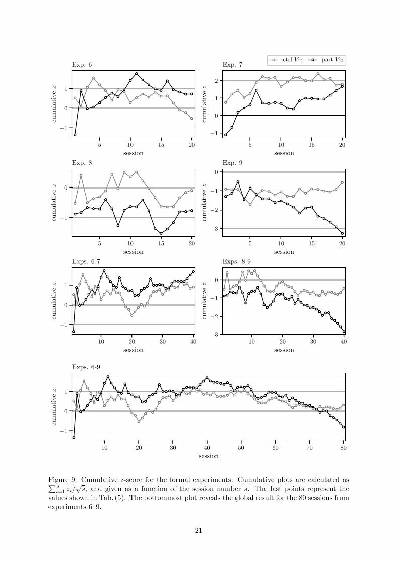
Table 5 summarizes the statistical results obtained for the intention/relax differential anal-ysis. For V1 and V2, statistical significance is found in participant data from exps. 7 and 9.However, a perplexing sign inversion is seen in exps. 8 and 9 participant data. The cumulativez-score plots for V12 presented in Fig. (9), highlights the sign inversion between the two N = 40blocks. While the combined exps. 8-9 is statistically significant, the sign reversions lead to aglobal exp. 6-9 non-significant result, both in the participant and control data.

3.6 Post hoc meta-analysis

In retrospect, the directional hypothesis being tested in the formal experiments is tighter thanthe original motivation of the study. While the primary hypothesis was concerned with absolutedifferences between intention and relax epochs, the tests performed in the formal studies wereimplicitly merged with a secondary hypothesis that the z-signs would be strictly associated withthe feedback-favored slit. As a post hoc meta-analysis, the two hypotheses of difference anddirection are decoupled into separate tests.

20

5 10 15 20

session

−1

0

1

cumulativez

Exp. 6

5 10 15 20

session

−1

0

1

2

cumulativez

Exp. 7ctrl V12 part V12

5 10 15 20

session

−1

0

cumulativez

Exp. 8

5 10 15 20

session

−3

−2

−1

0

cumulativez

Exp. 9

10 20 30 40

session

−1

0

1

cumulativez

Exps. 6-7

10 20 30 40

session

−3

−2

−1

0

cumulativez

Exps. 8-9

10 20 30 40 50 60 70 80

session

−1

0

1

cumulativez

Exps. 6-9

Figure 9: Cumulative z-score for the formal experiments. Cumulative plots are calculated as∑ s

i=1zi/

√s, and given as a function of the session number s. The last points represent the

values shown in Tab. (5). The bottommost plot reveals the global result for the 80 sessions fromexperiments 6–9.

21

V1 〈5− 15〉 V2 〈19 − 25〉 V12exp. N zp zc zp zc comp. zp zc esp esc

6 20 -0.22 0.54 -0.22 1.71 +V1 − V2 0.73 -0.54 0.16 -0.12

7 20 -1.37 -0.57 -2.17 -1.34 −V1 − V2 1.67 1.81 0.37 0.40

8 20 -1.53 -0.87 -0.30 -0.41 +V1 − V2 -0.77 -0.09 -0.17 -0.02

9 20 2.23 -1.21 3.00 1.48 −V1 − V2 -3.26 -0.56 -0.73 -0.13

6-7 40 0.81 0.78 1.69 -0.27 1.69 0.90 0.27 0.14

8-9 40 -2.66 0.24 -1.91 -0.75 -2.85 -0.46 -0.45 -0.07

6-9 80 -1.31 0.72 -0.16 -0.72 -0.81 0.31 -0.09 0.03

Table 5: Formal experiments’ results. The participant (control) sessions Stouffer’s z-score isdenoted as zp (zc), while effect size is denoted as esp (esc).

3.6.1 Difference test

The primary hypothesis is tested by applying Fisher’s method to the experiments’ results.According to this bi-directional method, the associated probabilities summed as −2

∑Ne ln pifollow a chi-squared distribution with 2Ne degrees of freedom, where Ne describes the numberof experiments being combined. Unlike with the Stouffer’s method, the z-sign plays no rolesince a two-tailed probability yields the same value for +z and −z.

The results for the Fisher combination are shown in Tab. (6) and Fig. (10), where the com-bined probabilities are converted back to standard scores. A remarkable significance is foundin the participant data, where all the controls conform to the null hypothesis. The effect sizesobtained in the exploratory and formal studies are consistent. Both variables V1 and V2 showsignificance, while their combination V12 reveals an effect size boost only in the participant data.

V1 〈5− 15〉 V2 〈19− 25〉 V12exps. zp zc esp esc zp zc esp esc zp zc esp esc2-5 3.05 0.08 0.30 0.01 2.32 0.29 0.23 0.03 4.17 0.62 0.42 0.06

6-9 1.95 0.63 0.22 0.07 2.53 1.59 0.28 0.18 2.75 0.72 0.31 0.08

2-9 3.30 0.17 0.25 0.01 3.16 0.97 0.24 0.07 4.73 0.60 0.35 0.04

Table 6: Statistical results obtained with Fisher’s method. Ne is respectively 4, 4 and 8 forexps. 2-5, 6-9 and 2-9.

e2-5 e6-9 e2-9

−0.2

−0.1

0.0

0.1

0.2

0.3

0.4

0.5

0.6

es

part V1 part V2 part V12 ctrl V1 ctrl V2 ctrl V12

Figure 10: Effect sizes for all experiments combined with Fisher’s method. The error barsrepresent the 95% confidence interval.

To achieve those results, the sessions’ differential z-scores are first combined, as usual, into

22

each experiment’s Stouffer z-score; then, the experiments’ z-scores are combined using Fisher’smethod. According to the literature, “the Stouffer test statistics is sensitive to consistent,even if mild, departures from null hypothesis in separate studies, whereas the Fisher proce-dure is most sensitive to occasional, extreme departures” [28, p. 66]. As stated, the use of aStouffer combination within an experiment is strategic, aiming to catch small but consistentintention/relax differences in the same direction. If the direction can be consistently predictedby the feedback-favored slit, that’s a secondary question detailed below.

3.6.2 Direction test

Two tests are performed to study the relationship between the obtained z-score signs and thefeedback-favored slit: binomial and correlation. Both analyses use the V1 and V2 z-scoresobtained in exps. 4-9, since they all share the same feedback variable. Experiments 4,6,8 and5,7,9 are considered separately due to their opposite feedback-favored slit. The tests results areshown in Tab. (7).

V1 binomial V2 binomial V1&V2 correlation

exps. n+p n+c pp pc n+p n+c pp pc rp rc pp pc

4,6,8 26 27 0.25 0.37 27 31 0.37 0.70 -0.32 0.04 0.01 0.74

5,7,9 27 23 0.37 0.05 29 29 0.70 0.70 0.33 -0.09 0.01 0.50

Table 7: First two columns: binomial tests for the V1 and V2 z-score signs. Third column:correlation between V1 and V2 z-scores.

In the binomial analysis, the number of positive z-score sessions n+ is statistically evaluatedaccording to a binomial distribution of N = 60 and p = 0.5. For N = 60 sessions, a number ofpositive z outcomes between 23 and 37 is expected as statistical fluctuation (with α = 5%). Asseen in the results table, no significant outcomes were found for any condition.

For the correlation analysis, the Pearson’s r is obtained for the V1 and V2 differential z-scores. Statistical significance is found for the participant data, providing interesting evidencefor the ψφ-interaction; in terms of absolute z-score value, both variables tend to result invalues of correlated magnitude, while the values found in the control data are uncorrelated.The results also show that the correlation signs are inverted between the two experimentalgroups, confirming the legitimacy of having used the V12 sign compositions. As the scoresare anti-correlated in exps. 4,6,8, the compound variable should follow the generic form ofV12 = ±(V1 − V2); and since in exps. 5,7,9 the scores are correlated, the variable is genericallyexpressed as V12 = ±(V1 + V2).

When decoupling the formal experiment into two hypotheses, one learns that significantintention/relax absolute deviations are consistently found in the participant data, while therelationship between the feedback-favored slit and the V1,2 variables is expressed by their cor-relation value rather than their absolute signs.

3.7 Environment variables

The differential analysis was also applied to the environment variables, and the resulting stan-dard scores are presented in Tab. (8), where global scores are combined using Fisher’s method.Two variables resulted in global statistical significance, the laser temperature TL and the CCDexternal temperature T2C . The latter one shows significance also for the control data, which isindicative of an artifact possibly related to analog-digital resolution and discrete temperaturejumps.

To determine whether those two variables, or any other, could be associated with the dif-ferences measured in the V1,2 variables of interest, the Pearson’s r correlation was calculated

23

TC TL TR |Mx| |My| |Mz|exp. zp zc zp zc zp zc zp zc zp zc zp zc

0 -0.08 0.41 0.22 0.12 0.88 0.24 -1.19 -0.30 0.30 0.46 2.22 -0.67

1 1.17 -0.33 -0.25 0.53 -0.70 -0.23 0.91 0.43 -0.34 -0.09 0.07 0.16

2 -0.69 0.91 -1.21 1.49 1.03 0.12 0.19 -0.23 0.70 -0.10 -0.83 -1.36

3 -1.14 1.28 3.14 -0.21 -1.61 1.35 -0.59 -1.07 -2.12 0.71 2.43 -0.18

4 -0.73 0.03 -0.68 -0.22 -0.15 0.18 -0.05 1.26 -0.10 -0.04 0.70 -0.70

5 -0.11 0.44 0.20 -1.09 -1.15 0.34 -1.24 -1.10 -1.53 0.98 -1.15 -0.63

6 -0.92 0.68 -0.66 0.32 0.01 -0.34 0.69 -0.46 0.18 -0.94 -0.12 0.10

7 0.20 0.14 -2.53 -1.06 -0.24 -0.50 -1.73 0.32 0.04 0.04 0.35 -1.06

8 0.47 0.49 -1.85 -1.61 1.36 0.87 0.35 -1.04 0.60 0.09 -0.01 0.97

9 0.26 -0.55 -1.67 -1.85 -0.46 0.04 -0.30 1.46 0.03 2.05 0.99 -0.62

1-9 0.22 0.10 2.93 1.12 0.55 0.04 0.37 0.67 0.41 0.25 0.71 0.26

T2C |M2x| |M2y| |M2z |exp. zp zc zp zc zp zc zp zc

4 -1.25 0.98 0.39 -1.26 1.00 -1.32 0.08 -0.14

5 0.19 -0.58 0.60 -0.21 1.54 -0.67 0.27 0.67

6 -2.08 1.89 1.08 -0.69 0.12 -0.13 0.63 -0.86

7 2.16 2.37 0.05 1.23 0.73 0.71 0.14 0.44

8 3.57 2.87 -0.60 0.28 -0.10 -0.39 -0.54 -0.02

9 4.34 4.46 -0.49 -0.03 0.25 -0.08 -0.76 0.54

4-9 5.23 4.94 0.16 0.33 0.36 0.21 0.04 0.07

Table 8: Differential z-score for the environmental variables throughout the experiments. Toinvestigate magnitude variations, the magnetic field components were transformed into theirabsolute values before analysis. Global scores are obtained with Fisher’s method.

between the 240 differential z-scores obtained for the V1,2 variables and the 240 differentialz-scores obtained for the environmental variables. The CCD internal temperature TC vs V1 wasthe only combination showing a statistically significant correlation in the participant data, withrp = −0.18, pp = 0.005; and rc = 0.04, pc = 0.49 for the controls.

No environmental variable resulted in both a global significant z-score and a significantcorrelation to the V1,2 differential z-score. This excludes the trivial explanation of temperatureor magnetic field variations in intention/relax conditions being the primary cause of the changesmeasured in the V1,2 variables. The correlation found for the camera temperature, if consistentlyfound in future studies, may be indicative of a physical signature resulting from the investigatedψφ-interaction.

4 Discussion

The exploratory experiments testing a consciousness-related form of interaction with a double-slit system resulted in a highly significant difference between the intention and relax conditions.The subsequent formal experiments then tried to replicate the previous findings, failing to reachglobal significance due to a sign inversion in the last two experiments. A post hoc meta-analysiscombining the formal experiments’ results independently of the standard score signs resulted ina statistically significant effect, revealing that the pre-registered hypothesis was more restrictivethan initially intended.

24

Concerning the formal experiments, one may claim that the globally non-significant resultreveals the expected nonexistence of the ψφ-interactions – that some statistical fluctuations mayhave occurred, but for a sufficiently large database the effects fade away. This interpretationis challenged mainly by the standard score magnitudes found in participant data as comparedwith the controls, what is quantitatively exposed by the Fisher test performed in the post hocanalysis. One must have in mind that under the no-interaction scenario, participant and controldata are understood as essentially equivalent.

A possible objection would be that the control and the participant data cannot be equallyclassified because of the participant’s bodily presence in the experimental room; hence heat,vibrations, and electromagnetic radiation would be responsible for the larger effect sizes. Whilethe body may slightly affect the measurements, it’s important to remember that the variableshave their trends corrected with an 8th order polynomial, and that the measured effect translatesa consistent difference between the detrended values obtained in the 40 alternated intention andrelax epochs.

Concerning the physical mechanisms that could lead to artifacts in the participant data, heatis a monitored quantity, and no sensor resulted in both a globally significant differential score anda significant correlation to the variables of interest. Also, in experiment 0 a lamp producingmore heat than a human body replaced the participant, demonstrating that a temperatureincrease in the experimental room cannot account for the measured effects. Vibrations andelectromagnetic influences are highly attenuated with the respective use of a vibration isolationtable and a Faraday’s cage. Even in the case of minor leakages, the oscillatory nature of vibrationis more likely to introduce noise into the measurements than a direction-consistent variationthat could mimic a signal; and if the participant can (according to their intention) modulate aelectromagnetic emission that affects the double-slit system, that itself is indicative of a noveltechnology.

Trying to hold to the no-interaction interpretation, one may claim that the exploratoryexperiments’ results are due to data dredging. The first response to this view is related tothe physical meaning of the variables of interest. The variables explored by the optimizationtechnique are theoretically justified by the mathematical model predicting the ψφ-interactionsignatures according to the system’s measured geometry. This is also important as it restricts thenumber of possible combinations, as opposed to a variable not bound to any physical meaning.

As a further rebuttal to the data-dredging argument, one faces again the participant/controlequivalence; if both datasets are equivalent, how likely is one to find such a big effect in onlyone of them while applying the exact same analysis to both? It is reasonable to ask if theresults could be somehow inflated, but in the absence of a legitimate interaction, the inflationshould equally affect both samples. The final response is of an empirical nature, and presentedby the so-called reverse study, where the author tried to deliberately hack the control datato artificially produce the largest possible intention/relax differences – a task which failed toproduce a statistically significant global effect.

In contrast, the post hoc meta-analysis results lead to an interpretation supporting the ψφ-interactions. The word meta is emphasized in the sense that it simply implements a differentway of combining the experiments’ global scores, where all the session scores are unaltered. Theintent of this post hoc analysis was to decouple the formally tested hypothesis into two differenttests: of an absolute difference between intention/relax conditions, and of a causal relationshipbetween the difference sign and the slit targeted in the feedback. One challenge faced by thisinterpretation is in terms of meaning; if one cannot control the effect sign obtained, what ishappening within the underlying physical process?

A possible argument in favor of the inability to control the light-enhanced slit is based onthe discrepancy between the variable used to provide feedback and the one used in the offlineanalysis. While the first variable is built using the Fourier magnitude component, the seconduses the phase. This difference is attributable to the author’s learning curve during the study,

25

and thus will be avoided in future studies. A more speculative explanation points to somesort of global conservation law underlying the phenomenon; while local significant differencesmay occur, globally and across time they show a tendency to cancel out. Knowing this, futurestudies can pre-register to combine the experiment’s results using the Fisher method.

The main obstacle for the ψφ-interaction interpretation concerns its controversial nature– the interaction shouldn’t exist according to the current scientific world view. Also, if theinteraction exists how could it have remained undetected given the technological breakthroughsof the last century? First, it’s reasonable to expect a small cross-section, an effect so small itwould go unperceived in people’s daily lives, that needs proper amplification and a group sampleto be statistically detected in a controlled setting. Second, being a function of the consciousagent subjective condition, it may rely on a specific state of consciousness and sufficient skill,thus not being consistently achievable by anyone in any situation. In particular, if the effecthappens to be catalyzed by states opposed to rational faculties such as thinking and the use oflanguage, it may lead to a paradoxical situation; the more one tries to exert control, the less theycause the phenomenon. A third reason can be advanced as a consequence of the socioculturalprocess described by [29, Chap. 1] that led physicists to shift from philosophical interests to amore pragmatic approach in response to post-world war II military interests. While it was notuncommon for the founding fathers of quantum physics to discuss topics such as consciousnessand mysticism, because of the post-war technological race, the interest in such topics not onlybecame old-fashioned but something to be avoided while following a “serious” career path. As aresult, the current consensus holds that consciousness is not necessary to describe the physicalworld, while not introducing consciousness per se in their experiments.

According to the Fisher’s method statistics, the exploratory experiments resulted in a 4.17sigma effect, while the formal experiments resulted in 2.75 sigma. Both experiments combinedproduce a value of 4.73 sigma. In contrast, the control experiments conformed to the nullhypothesis, showing that the obtained effect cannot be reduced to methodological or analyticalartifacts. The monitored environmental variables of temperature and magnetic field couldn’tbe assigned as the primary causal sources of the light-measured intention/relax differences.

The observed effect cannot be exclusively explained as a consequence of the participants’consciousness collapsing the photons’ wavefunctions. If that were the case, one would expect tosee a decrease in the interference component followed by a 50/50-balanced slit-intensity ratio.Instead, the results reveal a probability modulation enhancing the light passage through aspecific slit – the interaction can be pictured as a Maxwell’s demon kind of influence, whereintention plays the demon’s role by “steering” some photons to the desired left/right slit. Thusthe presented results don’t provide a solution to the quantum measurement problem; a similarview is shared by [30], and in Radin et al’s double-slit studies from 2015 onwards. From atheoretical perspective, it is more reasonable to interpret the measured effect as an interactionadding complex numbers to the path amplitudes which, by interference, leads to a change inthe outcome probabilities. Rather than challenging the quantum mechanics framework and thetraditional objective interpretations, the results suggest a standard-model violation, pointingto the existence of a still-to-be-elucidated fundamental force field.

Future improvements to the current double-slit setup can be achieved by implementingstrategies that improve the signal-to-noise ratio in the interference pattern measurements, andthat provide more reliable feedback information. Regarding the variable of interest, instead offringe visibility, the use of Fourier-transformed phase variables is suggested in order to benefitfrom the full CCD frame information. Concerning the study design, it’s recommended that theexperiment be started in an exploratory fashion, and move to formal studies when sufficientknowledge is gained from the apparatus. As a next step, it would be interesting to run a dis-tant version of the experiment, where the participants are situated outside of the experimentalroom when they receive the real-time feedback. From the theoretical side, refinements in theinteraction model can be sought in order to provide even sharper variable predictions. Consid-

26

ering the profound implications of the observed effect being confirmed as a legitimate anomaly,replication efforts are strongly advised.

5 Acknowledgements

The author gratefully thanks all of the participants involved in this research for dedicatingtheir time and attention to the experimental task. The author is also grateful to Dean Radin,for advice about conducting the experiment; Hartmut Grote, for helpful comments on earlierdrafts of this manuscript; Wellington Zangari, for discussions on the subject matter; MikiyaMuramatsu, for discussions on the physical properties of the optical system; and George Ortegaand Grant Norrie, for language revision.

References

[1] D. J. Chalmers, “Facing up to the problem of consciousness,” Journal of consciousness

studies, vol. 2, no. 3, pp. 200–219, 1995.

[2] J. Von Neumann, Mathematical foundations of quantum mechanics. No. 2, Princetonuniversity press, 1955.

[3] F. London and E. Bauer, “The theory of observation in quantum mechanics (1939),” inQuantum theory and measurement (J. A. Wheeler and W. H. Zurek, eds.), pp. 217–259,Princeton University Press, 1983.

[4] E. P. Wigner, “Remarks on the mind-body problem (1961),” in Quantum theory and mea-

surement (J. A. Wheeler and W. H. Zurek, eds.), pp. 168–181, Princeton University Press,2014.

[5] H. P. Stapp, “Mind, matter, and quantum mechanics,” Foundations of Physics, vol. 12,no. 4, pp. 363–399, 1982.

[6] E. J. Squires, “Quantum theory and the relation between the conscious mind and thephysical world,” Synthese, vol. 97, no. 1, pp. 109–123, 1993.

[7] B. Rosenblum and F. Kuttner, “The observer in the quantum experiment,” Foundations

of Physics, vol. 32, no. 8, pp. 1273–1293, 2002.

[8] B. d’Espagnat, “Consciousness and the wigner’s friend problem,” Foundations of Physics,vol. 35, no. 12, pp. 1943–1966, 2005.

[9] H. Margenau, “Measurements in quantum mechanics,” Annals of Physics, vol. 23, no. 3,pp. 469–485, 1963.

[10] H. D. Zeh, “On the interpretation of measurement in quantum theory,” Foundations of

Physics, vol. 1, no. 1, pp. 69–76, 1970.

[11] S. Goldstein, “Quantum theory without observers – parts one and two,” Physics Today,vol. 51, no. 3 and 4, pp. 42–46 and 38–42, 1998.

[12] M. Schlosshauer, J. Kofler, and A. Zeilinger, “A snapshot of foundational attitudes towardquantum mechanics,” Studies in History and Philosophy of Science Part B: Studies in

History and Philosophy of Modern Physics, vol. 44, no. 3, pp. 222–230, 2013.

[13] S. Yu and D. Nikolic, “Quantum mechanics needs no consciousness,” Annalen der Physik,vol. 523, no. 11, pp. 931–938, 2011.

27

[14] D. I. Radin and R. D. Nelson, “Evidence for consciousness-related anomalies in randomphysical systems,” Foundations of Physics, vol. 19, no. 12, pp. 1499–1514, 1989.

[15] H. Bosch, F. Steinkamp, and E. Boller, “Examining psychokinesis: the interaction of hu-man intention with random number generators–a meta-analysis.,” Psychological bulletin,vol. 132, no. 4, pp. 497–523, 2006.

[16] D. Radin, R. Nelson, Y. Dobyns, and J. Houtkooper, “Reexamining psychokinesis: com-ment on bosch, steinkamp, and boller (2006).,” Psychological bulletin, vol. 132, no. 4,pp. 529–532, 2006.

[17] M. Ibison and S. Jeffers, “A double-slit diffraction experiment to investigate claims ofconsciousness-related anomalies,” Journal of Scientific Exploration, vol. 12, no. 4, pp. 543–50, 1998.

[18] W. K. Wootters and W. H. Zurek, “Complementarity in the double-slit experiment: Quan-tum nonseparability and a quantitative statement of bohr’s principle,” Physical Review D,vol. 19, no. 2, p. 473, 1979.

[19] D. Radin, L. Michel, K. Galdamez, P. Wendland, R. Rickenbach, and A. Delorme, “Con-sciousness and the double-slit interference pattern: Six experiments,” Physics Essays,vol. 25, no. 2, p. 157, 2012.

[20] D. Radin, L. Michel, J. Johnston, and A. Delorme, “Psychophysical interactions with adouble-slit interference pattern,” Physics essays, vol. 26, no. 4, pp. 553–566, 2013.

[21] D. Radin, L. Michel, A. Pierce, and A. Delorme, “Psychophysical interactions with a single-photon double-slit optical system,” Quantum Biosystems, vol. 6, no. 1, pp. 82–98, 2015.

[22] D. Radin, L. Michel, and A. Delorme, “Psychophysical modulation of fringe visibility in adistant double-slit optical system,” Physics Essays, vol. 29, no. 1, pp. 14–22, 2016.

[23] A. Tellegen and G. Atkinson, “Openness to absorbing and self-altering experiences (”ab-sorption”), a trait related to hypnotic susceptibility.,” Journal of abnormal psychology,vol. 83, no. 3, p. 268, 1974.

[24] J. Goodman, Introduction to Fourier Optics. W. H. Freeman, third ed.

[25] S. Smith, Digital Signal Processing: A Practical Guide for Engineers and Scientists. Else-vier Science, 2003.

[26] G. Guerrer, “Pre-registration for experiments 6 and 7,” Open Science Framework, regis-

tration form, 2017, http://dx.doi.org/10.17605/OSF.IO/6WXV5.

[27] G. Guerrer, “Pre-registration for experiments 8 and 9,” Open Science Framework, regis-

tration form, 2017, http://dx.doi.org/10.17605/OSF.IO/9V4Z5.

[28] R. Abelson, Statistics As Principled Argument. Taylor & Francis, 2012.

[29] D. Kaiser, How the hippies saved physics: science, counterculture, and the quantum revival.WW Norton & Company, 2012.

[30] M. De Bianchi, “Quantum measurements are physical processes. comment on “conscious-ness and the double-slit interference pattern: Six experiments” by dean radin et al.,”Physics Essays, vol. 26, no. 1, pp. 15–20, 2013.

28

Supporting Information: Consciousness-related interactions in a double-slit

optical system

S1 Phase variable discontinuities

The method for transforming a CCD frame in a variable of interest was described in Section2.9. The present section details the strategies for avoiding artificial discontinuities that mayarise in the process.

When transforming a complex number from Cartesian to polar coordinates, the obtainedphase angles are confined to a −π . . . π interval. If the phase value is close to ±π, variation overtime may consequently result in a 2π discontinuity. It’s usually possible to detect and fix thejumps using an unwrap algorithm, as shown in Fig. (S1).

0 250 500 750 1000 1250

frame

−3.0

−1.5

0.0

1.5

3.0

Pk=15

before unwrapping

0 250 500 750 1000 1250

frame

−3.6

−3.4

−3.2

−3.0

−2.8

Pk=15

after unwrapping

Figure S1: An example in the Fourier phase component at k = 15 where unwrapping successfullyfixes the 2π discontinuities.

However, as shown in Fig. (S2), sometimes the algorithm fails in fixing the discontinuities.This occurs when the unwrap fails to detect a jump as a consequence of noise added to thephase values. As discussed in the digital signal processing literature [25, p. 166], the smallerthe magnitude associated with a certain k, the higher the phase noise. Thus, according tothe magnitude values shown in Fig. (2), in the current setup one expects to find more unwrap-surviving discontinuities in k between 10 and 40, than in k between 1 and 9.

0 250 500 750 1000 1250

frame

−3.0

−1.5

0.0

1.5

3.0

Pk=20

before unwrapping

0 250 500 750 1000 1250

frame

−30

−20

−10

0

Pk=20

after unwrapping

Figure S2: An example in the Fourier phase component at k = 20 where unwrapping fails tofix the 2π jumps, producing even larger discontinuities.

Discontinuities in the time series are bound to introduce artifacts in a differential analysis,

1

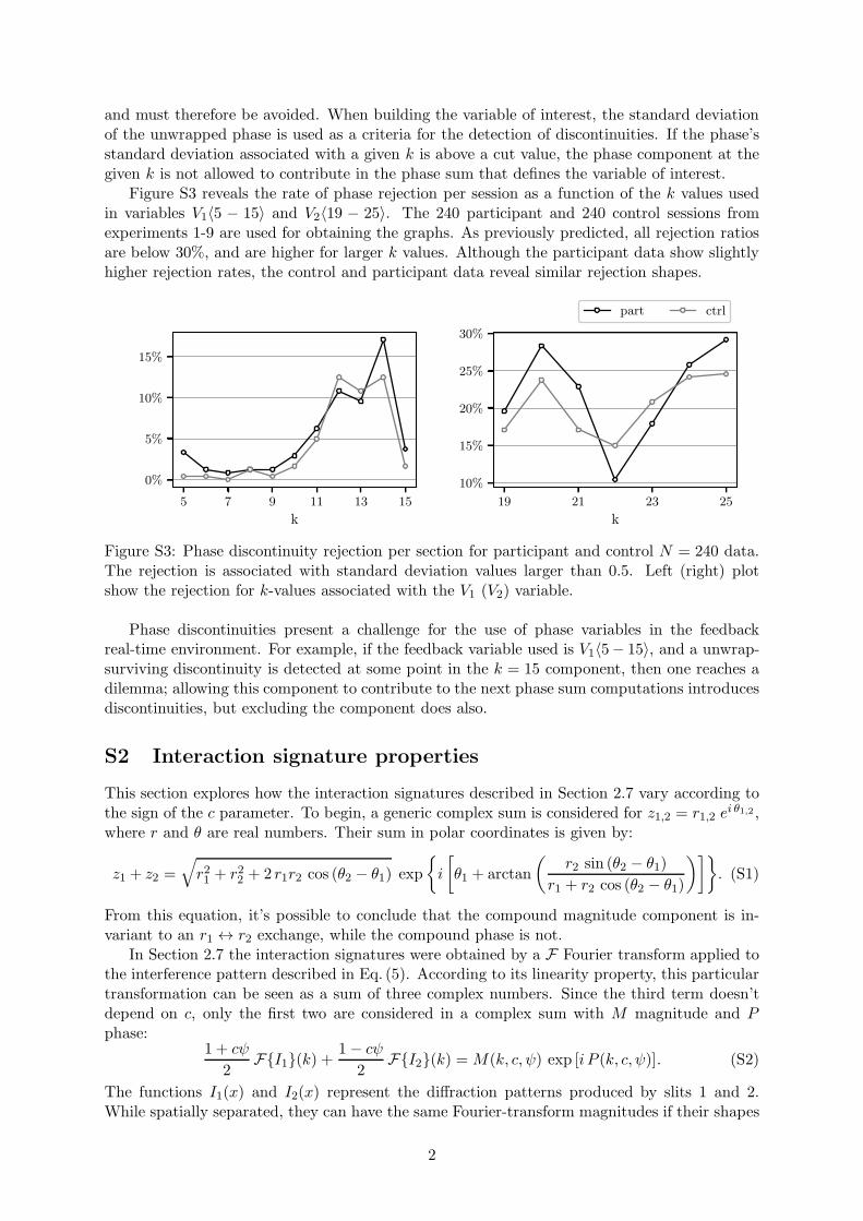
and must therefore be avoided. When building the variable of interest, the standard deviationof the unwrapped phase is used as a criteria for the detection of discontinuities. If the phase’sstandard deviation associated with a given k is above a cut value, the phase component at thegiven k is not allowed to contribute in the phase sum that defines the variable of interest.

Figure S3 reveals the rate of phase rejection per session as a function of the k values usedin variables V1〈5 − 15〉 and V2〈19 − 25〉. The 240 participant and 240 control sessions fromexperiments 1-9 are used for obtaining the graphs. As previously predicted, all rejection ratiosare below 30%, and are higher for larger k values. Although the participant data show slightlyhigher rejection rates, the control and participant data reveal similar rejection shapes.

5 7 9 11 13 15

k

0%

5%

10%

15%

19 21 23 25

k

10%

15%

20%

25%

30%

part ctrl

Figure S3: Phase discontinuity rejection per section for participant and control N = 240 data.The rejection is associated with standard deviation values larger than 0.5. Left (right) plotshow the rejection for k-values associated with the V1 (V2) variable.

Phase discontinuities present a challenge for the use of phase variables in the feedbackreal-time environment. For example, if the feedback variable used is V1〈5− 15〉, and a unwrap-surviving discontinuity is detected at some point in the k = 15 component, then one reaches adilemma; allowing this component to contribute to the next phase sum computations introducesdiscontinuities, but excluding the component does also.

S2 Interaction signature properties

This section explores how the interaction signatures described in Section 2.7 vary according tothe sign of the c parameter. To begin, a generic complex sum is considered for z1,2 = r1,2 e

i θ1,2 ,where r and θ are real numbers. Their sum in polar coordinates is given by:

z1 + z2 =√

r21 + r22 + 2 r1r2 cos (θ2 − θ1) exp

{

i

[

θ1 + arctan

(

r2 sin (θ2 − θ1)

r1 + r2 cos (θ2 − θ1)

)]}

. (S1)

From this equation, it’s possible to conclude that the compound magnitude component is in-variant to an r1 ↔ r2 exchange, while the compound phase is not.

In Section 2.7 the interaction signatures were obtained by a F Fourier transform applied tothe interference pattern described in Eq. (5). According to its linearity property, this particulartransformation can be seen as a sum of three complex numbers. Since the third term doesn’tdepend on c, only the first two are considered in a complex sum with M magnitude and Pphase:

1 + cψ

2F{I1}(k) +

1− cψ

2F{I2}(k) =M(k, c, ψ) exp [i P (k, c, ψ)]. (S2)

The functions I1(x) and I2(x) represent the diffraction patterns produced by slits 1 and 2.While spatially separated, they can have the same Fourier-transform magnitudes if their shapes

2

are identical. In such a scenario, it’s possible to show thatM(−c) =M(c), i.e. the impossibilityof discriminating the specific slit 1 or 2 associated with a ψ effect. The demonstration followsfrom using Eq. (S1) to obtain M(k, c, ψ), and realizing that the r1 ↔ r2 exchange correspondsto a c sign inversion if the I1 and I2 magnitude components are identical.

Alternately, differences between I1 and I2 shapes can produce asymmetries that enable oneto discriminate the specific slit 1 or 2 associated with a ψ effect. The shape differences can becaused by two conditions: a)s1 6= s2, or, different slit widths; b) Ur 6= 1, or, a different amount oflight crossing each slit. Condition b) is a consequence of a), but it can also be enhanced by smallrotations of the double-slit plane. Both conditions are met for the current setup, as shown inTab. (1). For Ur < 1, one finds thatM(−c) < M(c), and, consequently,M(−c)−M(0) < 0 whileM(c)−M(0) > 0. The last two inequalities, that are an approximation to Eq. (6) describing thedifference signatures, show that it’s possible to obtain positive or negative magnitude differencesfor a respective slit 1 or 2 light intensity enhancement.

For the P (k, c, ψ) phase component, no asymmetries are necessary to discriminate between±c. As previously shown, the compound phase is naturally asymmetric to an r1 ↔ r2 exchange.Thus even for identical magnitudes one obtains P (−c) < P (c), and, consequently, the positiveor negative differences for ±c shown in Fig. (4).

3