consanguinity and other marriage market effects of a ...€¦ · consanguinity and other marriage...

Consanguinity and Other Marriage Market Effectsof a Wealth Shock in Bangladesh

Ahmed Mushfiq Mobarak & Randall Kuhn & Christina Peters

Published online: 26 April 2013# Population Association of America 2013

Abstract This paper uses a wealth shock from the construction of a flood protectionembankment in rural Bangladesh coupled with data on the universe of all 52,000marriage decisions between 1982 and 1996 to examine changes in marital prospectsfor households protected by the embankment relative to unprotected householdsliving on the other side of the river. We use difference-in-difference specificationsto document that brides from protected households commanded larger dowries,married wealthier households, and became less likely to marry biological relatives.Financial liquidity-constrained households appear to use within-family marriage (inwhich one can promise ex-post payments) as a form of credit to meet up-front dowrydemands, but the resultant wealth shock for households protected by the embankmentrelaxed this need to marry consanguineously. Our results shed light on the socioeco-nomic roots of consanguinity, which carries health risks for offspring but can alsocarry substantial benefits for the families involved.

Keywords Marriage . Embankment . Flood protection . Consanguinity

Introduction

A woman’s marital prospects have important implications for her subsequent life out-comes. Conditions of marriage—such as dowries, marrying biological relatives, age at

Demography (2013) 50:1845–1871DOI 10.1007/s13524-013-0208-2

Electronic supplementary material The online version of this article (doi:10.1007/s13524-013-0208-2)contains supplementary material, which is available to authorized users.

A. M. Mobarak (*)School of Management, Yale University, 135 Prospect Street, P.O. Box 208200, New Haven, CT06520-8200, USAe-mail: [email protected]

R. KuhnJosef Korbel School of International Studies, University of Denver, Denver, CO, USA

C. PetersDepartment of Economics, Metropolitan State University of Denver, Denver, CO, USA

http://dx.doi.org/10.1007/s13524-013-0208-2

marriage, and spousal wealth—affect socioeconomic outcomes for the woman and herchildren, including the likelihood that she will have to endure domestic violence, herstatus in her husband’s home, her health and scholastic attainment, and her control overreproductive choices (Bloch and Rao 2002; Field and Ambrus 2008; Jahan 1990; Jensenand Thornton 2003; Tiemoko 2001; Wickrama and Lorenz 2002). Marrying a cousin oruncle—a surprisingly common practice around the developing world, accounting formore than 50 % of all unions in some countries—can decrease the amount of dowryrequired but increases the risk of genetic diseases among offspring. Understanding thedeterminants of these conditions of marriage is thus important.

In this article, we study the construction of a flood protection embankment in ruralBangladesh coupled with pre- and post-embankment data on 33,000 marriages toexamine how a plausibly exogenous change in wealth manifests itself in changes tomarriage conditions. This embankment induced a discrete improvement in socioeco-nomic conditions for families living on the embankment side of the river relative tothe opposite bank that remained unprotected. Its major effect was to extend the crop-growing season, thereby increasing wealth for households on the protected side. Weinvestigate differential changes in the conditions of marriage for protected householdsusing panel data on the entire universe of marriages in treatment and control villagesacross a 14-year period pre- and post-embankment.

Marrying a biological relative1 increases the likelihood that offspring willreceive two copies of a deleterious gene from parents, which results in highermorbidity and mortality rates (Bittles and Makov 1988; Shah et al. 1998).Social scientists have a limited understanding of why so many couples acceptthese risks. We use difference-in-differences (DD) analysis coupled with theexogenous variation in wealth to test some implications of a model of consan-guinity as a response to credit constraints (Do et al. forthcoming). We provideevidence that marrying consanguineously reduces the need for dowry payments.Because a bride’s parents often have neither cash on hand nor access to creditto make an up-front dowry payment, they use within-family marriage (where itbecomes possible to promise ex-post payments) as a form of credit. Given thatprotection from flooding increases wealth, the need for consanguineous mar-riage is reduced for protected households following embankment construction.

Our article thus contributes to a literature that attempts to uncover theeconomic motivations behind specific marriage practices, such as polygyny(Gould et al. 2008; Jacoby 1995), endogamy (Edlund 1999), dowry (Botticiniand Siow 2003), and exchange marriage (Jacoby and Mansuri 2010). Ourarticle also fits in a literature that studies the effects of policy changes andshocks on longer-run intrahousehold marriage and social outcomes (e.g.,Ambrus et al. 2010; Deininger et al. 2010). Finally, this article is also relatedto an emerging empirical literature on the determinants of spousal matching(Banerjee et al. 2009; Hitsch et al. 2010; Wong 2003).

1 In the mainly Muslim countries of North Africa and West and Central Asia, and in large parts of SouthAsia, marriages between close relatives account for between 20 % to 50 % of all unions, with an additional2.8 billion people in countries where 1 % to 10 % of marriages are between biological relatives (http://www.consang.net). Cousin marriage appears to be a social norm in Pakistan, Afghanistan, Iraq, and Yemen,where about 50 % of marriages are between first cousins (Bittles 1994, 2001; Caldwell et al. 1983; NewYork Times 2003; Rowlatt 2005).

1846 A.M. Mobarak et al.

http://www.consang.net

http://www.consang.net

The key identifying assumption underlying our DD empirical strategy is that changesin marriage patterns over time on the unprotected side of the river constitute a validcounterfactual for the changes in marriage patterns on the protected side. We establishthe credibility of this strategy by examining baseline differences in outcomes andcommon pretreatment trends. We check sensitivity of results to household fixed-effects analysis (using the subset of families with multiple marriages before and afterembankment construction) as well as on collapsed data (one pre-embankment and onepost-embankment observation) that minimizes serial correlation (Bertrand et al. 2004).All our specifications add fixed effects for every year of analysis so that the effects wereport are identified from a discrete jump tied to embankment construction, controllingfor the longer-term trend.

The next section builds on the literature on marriage and family to developtheoretical expectations of the effects of embankment construction on marriage out-comes more broadly and on consanguinity in particular. We then describe the settingand our data sources. Following that, we present empirical results that test ouridentification assumptions, showing how the embankment affects first-stage econom-ic outcomes. We then present results on a broad set of marriage outcomes: dowries,age at marriage, and spousal wealth. After we document the changes to consanguinityrates and try to uncover the structural changes that led to the large drop in consan-guinity, we conduct sensitivity analyses and offer conclusions.

Theory

Studies of marriage in the developing world continue to be shaped by William J.Goode’s theory of modernization and marital change (Goode 1963). Goode arguedthat the waning power of families in dictating the conditions of marriage would leadto the demise of traditional marriage patterns, including early female age at marriage,large age gaps between spouses, dowry or other wealth transfers at the time ofmarriage, and marriage between blood relatives. Subsequent research found consid-erable support for the decline of some traditional marriage patterns, most notablyearly marriage (Mensch et al. 2005). Yet, the institution of dowry has proven resilientand even resurgent in many parts of the world, particularly in South Asia (Anderson2007; Caldwell et al. 1983; Rao 1993). Consanguinity has also remained resilient inspite of the adverse biological risks for children (Grant and Bittles 1997).

In part, the resilience of traditional marriage practices derives from the persistentrole of families in marital decisions and in the postmarital social and economic life ofmarried couples (Rosenzweig and Stark 1989). Economic theory highlights themarriage matching process based on costs and benefits to marital partners and theirfamilies (Becker 1973, 1991). Caldwell et al. (1983) described these dynamics from ademographic and anthropological tradition, highlighting the role of marriage trans-actions in providing economic security. The literature has since tried to model variousconditions of marriage, including dowry (Rao 1993), consanguinity (Givens andHirschman 1994), spousal wealth and occupation (Fafchamps and Quisumbing2005; Rosenzweig and Stark 1989), and spousal education (Esteve and McCaa2008; Han 2010), allowing for asymmetric effects by gender (Amin and Cain 1997;Protik and Kuhn 2006).

Consanguinity and Other Marriage Market Effects of Wealth Shock 1847

Theoretical Model

We develop stylized two-sided matching models to help frame how the wealth and riskmitigation benefits of the embankment affect marriage decisions. Banerjee et al. (2009),Hitsch et al. (2010), and Wong (2003) have used information from online dating sitesand newspaper advertisements to demonstrate that such models can simulate actualoutcomes quite well. We discuss the basic predictions of the models here, and OnlineResource 1 provides details on our two-step modeling approach to describe matcheswhen multiple attributes of embankment protection can affect outcomes:

1. We derive analytical predictions on matching in a marriage market where eachperson has only two discrete attributes: embankment protection status and wealthstatus. To generate analytical solutions, we follow the literature (e.g., Siow 1998;Weiss 1997), and assume that there exists a medium of exchange (such as dowry)that can be used to transfer utility from the bride to the groom.

2. We then relax this assumption on transferable utility, endow each person withmultiple continuous characteristics, and simulate stable matches in a largermarriage market characterized by search frictions.

These models predict that the protected are likely to secure better matches onlyalong characteristics that are complementary. For example, if the wealth that a manand woman bring to a marriage represents complementary inputs toward generatingmarital surplus, then those living on the protected side would, in general, choose (andbe able) to marry into wealthier households. However, characteristics that are notcomplementary inputs— such as age at marriage or age gaps—should remain unaf-fected because the protected are not willing to pay relatively more than the unpro-tected for this characteristic. Furthermore, if the embankment’s primary contributionis to lower flood risk exposure, we should observe negative assortative matching inprotection post-embankment (i.e., more cross-river marriages). The unprotected havethe largest marginal gain from bonding with a protected family, and are thereforewilling to pay the most to secure that match. Search frictions across the river maydampen this effect. A corollary is that protected men should receive larger dowries.These simple matching models are useful for interpreting the basic DD programevaluation results, but they do not attempt to model consanguinity.

Consanguinity

Consanguinity remains a surprisingly common practice in much of the developingworld, even though the genetic risks for the offspring of the union of biologicallyclose relatives are well understood in the scientific community (Bittles and Neel1994; Grant and Bittles 1997; New York Times 2003). Estimates of excess birthdefects in first cousin progeny have ranged from 0.7 % to 7.5 % (Zlotogora 2002).Given these health risks, it is important to understand why so many households marrybiological relatives.

The socioeconomic benefits associated with consanguineous marriage may help toexplain its prevalence despite the documented health risks. The literature speculatesabout various reasons why marriage to a biological relative may be preferred,including a strong family tradition, lower spousal search and matching costs,


strengthening of family ties, closer relationships between the wife and her in-laws,greater autonomy for women, lower risk of divorce, and property retention within afamily (Bittles 1994; Sandridge et al. 2010). Caldwell et al. (1983) and Bittles (1994)have suggested that households marry within the family in South Asia to avoid largedowry payments at the time of marriage. Do et al. (forthcoming) modeled a marriagemarket failure in which families pledge wealth to improve the quality of the match butcannot credibly commit to future transfers. An ex ante transfer (dowry) or a consan-guineous marriage contract between relatives for whom a long-term contract isenforceable are two substitute solutions to the market failure.2 Families facing acredit constraint (who find it more expensive to pay dowries) would be more likely toengage in consanguinity as a way to delay payments. The promise to pay over alonger period is more credible when made within the family.

An exogenous shock to wealth that relieves the liquidity/credit constraint (such asthat afforded by the embankment) creates a natural experiment that allows us to testthe central implication of this model. We do so by constructing a DD estimate ofchanges in consanguinity in protected and unprotected areas before and after con-struction of the embankment. Furthermore, because the liquidity constraint binds onlythe bride’s family (because only the bride pays dowry), gender-disaggregated analysisof the embankment’s effect provides a triple-difference test of this implication.Although we show evidence in favor of a few specific reduced-form implicationsof this model, other models of the marriage market may yield the same types ofrelationships among wealth, consanguinity, and dowries.

Setting and Data

Since 1963, the International Centre for Diarrhoeal Disease Research, Bangladesh(ICDDR,B) has conducted periodic socioeconomic censuses and recorded all vitalevents of residents in 148 villages in Matlab district. During the study period,residents of this rural area were mostly poor and landless, subsisting off fishing,agricultural labor, and sharecropping.

Using ICDDR,B data, we observe all 33,000 marriages (or 52,000 marriagedecisions) of Matlab residents between 1982 and 1996, and we merge census datafrom 1982 to these marriage files. Note that these are demographic surveillance data(on the basis of visiting all households in the surveillance area on a frequent basis),and we therefore observe all marriages, regardless of where that marriage is regis-tered. When a Matlab resident marries someone outside the district, we observe thatmarriage but only from one side.3 A within-Matlab marriage is observed from both

2 Conversations during our fieldwork in rural Bangladesh in 2006 also indicated that sometimes this long-term contractual solution is mediated by the intergenerational link in inheritance, which makes the contracteasier to enforce. A male cousin may agree to marry a cousin who cannot afford to pay dowries on thepromise of a larger future bequest by the grandfather.3 Consanguinity status is not recorded in such cases. This is potentially an important selection issue, and weverify that there is no statistically significant difference in an indicator for “missing consanguinityinformation” across protected and unprotected areas either overall (p value = .29), or during the pre-embankment period. This variable is not significantly affected by embankment construction (protected ×post) either.


sides. We know the age at marriage of each individual and his or her spouse; anybiological relationship between them (i.e., consanguinity status); and their wealth(including landownership), occupation, and location (and, therefore, embankmentprotection status).

We supplement these data with retrospective dowry information, cropping prac-tices, and land value information reported in the 1996 Matlab Health andSocioeconomic Survey (MHSS; Rahman et al. 1996). The MHSS cross-sectionaldata set, which covers a random subsample of more than 4,000 householdsfrom Matlab, asks all respondents to recall dowries exchanged during pastmarriage transactions (thus covering marriages both before and after embankmentconstruction). We use the estimated cash value of dowries as reported by women whoare interviewed separately from their husbands. Table S1 in Online Resource 1 lists thevariables used in this study and their definitions.

The Meghna-Dhonagoda Embankment: First-Order Effects and Validityas a Natural Experiment

The Meghna-Dhonagoda River runs through the middle of the study area, and theWater and Power Development Authority in Bangladesh used external donor funds in1987 to construct a 65 km embankment along the northwest bank (see Fig. 1) thatprevents water overflow and provides systems for pumped drainage and irrigationalong the waterway (Strong and Minkin 1992). The embankment was breachedduring abnormally high floods in 1987 and 1988, after which it was strengthenedand resealed in 1989. Consequently, in our empirical specifications, the pre-embankment period is 1982–1986, and the post-embankment period covers 1989–1996. Before establishing the first-order effects of the embankment on wealth, weexamine whether the embankment can be treated as an exogenous shock.

What the Embankment Construction Helps Identify

The most important concern is that people residing on the southeast bank of the riverare not an appropriate control group for the “treated” households because theplacement of the embankment on the northwest bank may itself signal somepreexisting differences between the two groups.

During fieldwork interviews we conducted in 2006, Matlab residents indi-cated that the embankment was placed on the northwest side mainly becausedrainage was worse in that bank prior to embankment construction. Residentsalso expressed complaints that the project was coordinated by politicians inconjunction with the largest local landowners who actually live in Dhaka(Briscoe 1998; Kabir 2004). Neither politicians nor large landowners are partof our sample because they do not live in Matlab district. However, other formsof preferential treatment for the protected side of the river may be possible, andwe therefore delve into the program evaluation and anthropological literaturesto examine these issues.

One possibility is that agriculture practices are systematically different across thetwo banks because of drainage differences. However, program evaluations of the


embankment project report that the geographic areas experienced similar weatherpatterns, households grew similar crops and reported similar incomes, and demo-graphic distributions were nearly identical. Furthermore, we find no mention of anyother significant differences in technology or other construction, such as bridges, thatmay have happened to coincide with embankment construction (Briscoe 1998; Strongand Minkin 1992; Thompson and Sultana 1996).4 Descriptive statistics from our owndata show that the protected and unprotected groups are similar prior to constructionalong most observable dimensions (see Table 1). We present statistical test of

4 Because Matlab is part of a demographic surveillance area run by the International Centre for DiarrhealDisease Research (ICDDR,B), the population has been exposed to some development programs. Ourresults are robust to controlling for exposure to the largest of these programs, the Matlab Maternal andChild Health and Family Planning program and the Safe Motherhood Initiative.

Fig. 1 Matlab Surveillance Area, the river and the embankment. The light gray polygons are villages, thedouble line is the river, and the thin line is the embankment


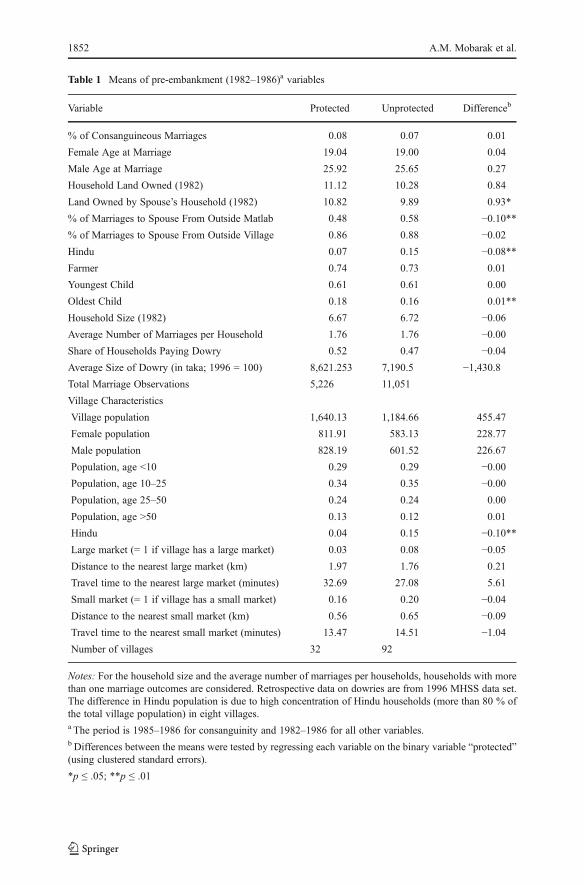
Table 1 Means of pre-embankment (1982–1986)a variables

Variable Protected Unprotected Differenceb

% of Consanguineous Marriages 0.08 0.07 0.01

Female Age at Marriage 19.04 19.00 0.04

Male Age at Marriage 25.92 25.65 0.27

Household Land Owned (1982) 11.12 10.28 0.84

Land Owned by Spouse’s Household (1982) 10.82 9.89 0.93*

% of Marriages to Spouse From Outside Matlab 0.48 0.58 −0.10**% of Marriages to Spouse From Outside Village 0.86 0.88 −0.02Hindu 0.07 0.15 −0.08**Farmer 0.74 0.73 0.01

Youngest Child 0.61 0.61 0.00

Oldest Child 0.18 0.16 0.01**

Household Size (1982) 6.67 6.72 −0.06Average Number of Marriages per Household 1.76 1.76 −0.00Share of Households Paying Dowry 0.52 0.47 −0.04Average Size of Dowry (in taka; 1996 = 100) 8,621.253 7,190.5 −1,430.8Total Marriage Observations 5,226 11,051

Village Characteristics

Village population 1,640.13 1,184.66 455.47

Female population 811.91 583.13 228.77

Male population 828.19 601.52 226.67

Population, age <10 0.29 0.29 −0.00Population, age 10–25 0.34 0.35 −0.00Population, age 25–50 0.24 0.24 0.00

Population, age >50 0.13 0.12 0.01

Hindu 0.04 0.15 −0.10**Large market (= 1 if village has a large market) 0.03 0.08 −0.05Distance to the nearest large market (km) 1.97 1.76 0.21

Travel time to the nearest large market (minutes) 32.69 27.08 5.61

Small market (= 1 if village has a small market) 0.16 0.20 −0.04Distance to the nearest small market (km) 0.56 0.65 −0.09Travel time to the nearest small market (minutes) 13.47 14.51 −1.04Number of villages 32 92

Notes: For the household size and the average number of marriages per households, households with morethan one marriage outcomes are considered. Retrospective data on dowries are from 1996 MHSS data set.The difference in Hindu population is due to high concentration of Hindu households (more than 80 % ofthe total village population) in eight villages.a The period is 1985–1986 for consanguinity and 1982–1986 for all other variables.b Differences between the means were tested by regressing each variable on the binary variable “protected”(using clustered standard errors).

*p ≤ .05; **p ≤ .01


differences prior to embankment construction at the level of variation in the data thatwe will use for our analysis (clustered by village), finding no significant differences atbaseline in terms of the consanguinity rate, male and female ages at marriage,landownership, the propensity to marry outside the village, household size, or numberof marriages per household. We also report statistical tests based on a large set offactors from the 1996 MHSS—such as share of households paying dowry; averagesize of dowry; village demographics; and location, distance from, and access tomarkets—and find no statistical differences between the protected and unprotectedset of villages.

Spousal landownership exhibits a statistically significant difference, and themagnitude of this difference is about 8 % of the average sample value. Becauseour DD estimation strategy will rely on relative changes in marriage outcomesacross the protected and unprotected banks between pre- and post-embankmentperiods, it is important to examine whether the assumption of “parallel trends”holds for this variable. Table 2 conducts a rigorous version of this test byrunning regressions of the following form for the two to five years of data priorto embankment construction:

Outcome Y Protectedit t t t( ) = + + + +− − −γ γ γ β5 4 1 0 . . . (( )i

+ ( ) ⋅ + ( ) ⋅ +−−β γ β γ5 45 4Protected Protectedi t i t . . . + ( ) ⋅ +−β γ 11 Protected e

i t .

The set of interaction terms between the indicator for a household living on theside of the river where the embankment will be built (Protected)i with a dummyvariable for each pre-embankment year is the most flexible way to look for differ-ences in the trends in preconstruction characteristics across the two sides of the river.In four of the five pre-embankment years, there is no statistical difference in spousallandownership between the two banks, and the point estimates go in both directions,depending on the year. The pre-embankment difference in spousal landownershipfrom Table 1 is entirely driven by just one unusual year of data. We also conduct amore simple linear trends test and verify that there is no statistically significantdifference in the linear trend across the two banks of the river during the pre-embankment period.

Table 2 also shows that protected and unprotected trends in the consanguin-ity rate prior to embankment construction are not statistically different, and themagnitudes of the differences are very small when compared with the actualembankment effect estimates we present later.5 Any relative changes in trendspost-embankment that our DD estimates uncover are therefore not merely acontinuation of preexisting differences in trends. There is also no clear trend indowries during the pre-embankment period.

5 Fig. S3 in Online Resource 1 graphs the pre- and post-embankment consanguinity rates. Consanguinityfalls on both sides of the river in the year prior to embankment construction, but there is no differentialdecrease on the protected side. Moreover, the preexisting trends are also not statistically different whenbroken down by gender (results available upon request).


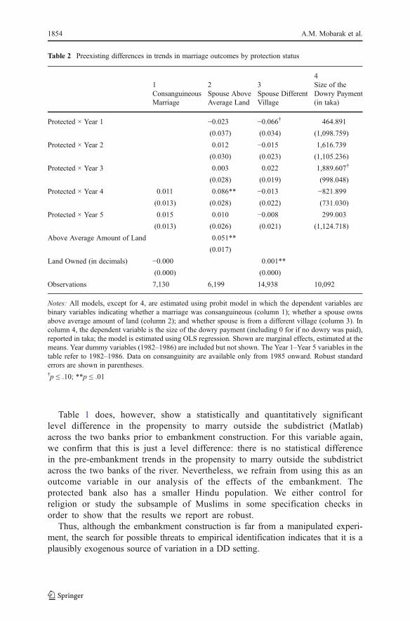
Table 1 does, however, show a statistically and quantitatively significantlevel difference in the propensity to marry outside the subdistrict (Matlab)across the two banks prior to embankment construction. For this variable again,we confirm that this is just a level difference: there is no statistical differencein the pre-embankment trends in the propensity to marry outside the subdistrictacross the two banks of the river. Nevertheless, we refrain from using this as anoutcome variable in our analysis of the effects of the embankment. Theprotected bank also has a smaller Hindu population. We either control forreligion or study the subsample of Muslims in some specification checks inorder to show that the results we report are robust.

Thus, although the embankment construction is far from a manipulated experi-ment, the search for possible threats to empirical identification indicates that it is aplausibly exogenous source of variation in a DD setting.

Table 2 Preexisting differences in trends in marriage outcomes by protection status

1ConsanguineousMarriage

2Spouse AboveAverage Land

3Spouse DifferentVillage

4Size of theDowry Payment(in taka)

Protected × Year 1 −0.023 −0.066† 464.891

(0.037) (0.034) (1,098.759)

Protected × Year 2 0.012 −0.015 1,616.739

(0.030) (0.023) (1,105.236)

Protected × Year 3 0.003 0.022 1,889.607†

(0.028) (0.019) (998.048)

Protected × Year 4 0.011 0.086** −0.013 −821.899(0.013) (0.028) (0.022) (731.030)

Protected × Year 5 0.015 0.010 −0.008 299.003

(0.013) (0.026) (0.021) (1,124.718)

Above Average Amount of Land 0.051**

(0.017)

Land Owned (in decimals) −0.000 0.001**

(0.000) (0.000)

Observations 7,130 6,199 14,938 10,092

Notes: All models, except for 4, are estimated using probit model in which the dependent variables arebinary variables indicating whether a marriage was consanguineous (column 1); whether a spouse ownsabove average amount of land (column 2); and whether spouse is from a different village (column 3). Incolumn 4, the dependent variable is the size of the dowry payment (including 0 for if no dowry was paid),reported in taka; the model is estimated using OLS regression. Shown are marginal effects, estimated at themeans. Year dummy variables (1982–1986) are included but not shown. The Year 1–Year 5 variables in thetable refer to 1982–1986. Data on consanguinity are available only from 1985 onward. Robust standarderrors are shown in parentheses.†p ≤ .10; **p ≤ .01


First-Order Effects of the Embankment on Income, Wealth, and Risk

Before turning to marriage outcomes, we examine the first-order effects of embank-ment construction on economic outcomes using regressions of the form

Y Protected Post Post Protectedit i t= + ( ) + ( ) + ×α β β β1 2 3(( ) +

it ite

whenever we have panel data, or

Y Protected eit i i= + ( ) +α β1

for any outcome for which we have only cross-sectional data.Frequent flooding in Matlab destroys crops and induces volatility in household

income, and the embankment provides security by extending growing seasons andincreasing farm incomes for protected agricultural households. During fieldwork weconducted in December 2006, Matlab residents often reported that the primary effectof the embankment was to increase the number of crop cycles from only one percalendar year to two or three because the monsoon swelling of rivers would encroachon the agricultural land as long as three to five months per year prior to embankmentconstruction. Consistent with these informal interviews, Matlab data from 1996indicate that protected rice farmers enjoyed almost one extra growing season percalendar year compared with farmers on the other side of the river (t test significant atthe 1 % level). Thompson and Sultana (1996) mentioned that the largest effects offlood protection projects should be on monsoon crops, and accordingly, our datashow that protected farmers grew 2–3 times more Aman and Aus paddy (the twovarieties grown during the monsoon) per decimal of cultivated land compared withunprotected farmers (t tests significant at the 5 % level). Meanwhile, the embankmenthad no discernible effect on yields for the dry season Boro paddy.

Protected farmers should become wealthier from these large increases in riceyields. We measure this effect directly by using principal components analysisto construct asset indices for household wealth in 1982 and 1996 (seeTable 3).6 Compared with unprotected households, protected households expe-rienced a greater increase (significant at the 5 % level) in asset ownershipbetween 1982 (pre-embankment) and 1996 (post-embankment). Moreover, thischange was driven almost entirely by farmers.7 A hedonic regression of thevalue of land using cross-sectional 1996 data reveals that post-embankment, theunit price of land was more than 3,000 taka higher per decimal on the

6 The index measures household ownership of the following assets: a radio, a watch or clock, a bicycle,cows, and a hurricane lamp. Data are taken from Matlab DSS 1982 and 1996 household censuses.Occupation of household head is kept as reported in 1982.7 Both landowners and tenant farmers benefited in significant ways, which indicates that the extendedgrowing season on the protected side probably increased both the productive capacity of land as well as thedemand for agricultural labor. From Table 3, it may appear that the effect on tenants was larger than that onlandowners, but this is because the index is capped when an individual reports owning all such items.Wealthier landlords attained the maximum value even pre-embankment, and the change in their index valuewas therefore smaller.


protected side.8 The variance of assets across households within a village(which would be linked to changes in risk exposure) did not differentiallychange across the protected or unprotected banks (see Table S2 in OnlineResource 1). Consistent with the fieldwork findings, the mean wealth effectof the embankment thus appears to dominate changes in variance.

In summary, we find that gains in wealth were likely the most salient change andthe dominant embankment effect for protected Matlab residents. Thus, we focus onidentifying the effects of wealth changes in our empirical analysis. Photographs inOnline Resource 1 (Fig. A2) show that the embankment is not a soaring barrier thatcan protect residents from the gushing floodwaters that are an enduring risk to life andproperty periodically faced by rural Bangladeshis. Rather, it is a more modest barrierdesigned to protect agricultural fields from seasonal variation in water levels thatrender those fields inarable during the monsoons. The data on cropping cycles,agricultural yields, land values, and wealth by occupation all indicate that theembankment performs this limited function well, bestowing a positive wealth shockon protected households and particularly on farming households.

8 These results are available upon request. Control variables for this regression include total land area underirrigation, distance to nearest market, travel time to nearest market, whether the village has a creditinstitution, whether the village participates in the MCHFP program, and controls for area under cultivationand cost of cultivation by crop type.

Table 3 Effects of the embankment on wealth using census data

Growth in the Asset Index1982–1996

Protected Unprotected

DifferenceAcross Protected/Unprotected

All Occupations Mean 0.39 0.3 0.085*

SE (0.02) (0.01) (0.04)

Observations 5,460 11,656 17,116

Non-FarmOccupations

Mean 0.26 0.26 −0.0004SE (0.03) (0.02) (0.07)

Observations 1,530 3,207 4,737

Farmers(Landowners)

Mean 0.43 0.34 0.092†

SE (0.02) (0.02) (0.048)

Observations 3,378 7,270 10,648

Farmers (Tenant) Mean 0.5 0.23 0.278**

SE (0.05) (0.03) (0.01)

Observations 552 1,179 1,731

Notes: The asset index is constructed through principal components factor analysis and measures householdownership of any combination of the following assets: radio, watch or clock, bicycle, cows, and a hurricanelamp. Data are taken from Matlab DSS 1982 and 1996 household censuses. The test of differences acrossprotected/unprotected sides of the river clusters standard errors by village.†p ≤ .10; *p ≤ .05; **p ≤ .01


Effects of the Embankment on Marriage Outcomes

Estimation Strategy

Our DD setup compares the marriage market outcomes for protected householdsfollowing embankment construction to their pre-embankment outcomes, afterdifferencing out the corresponding change in unprotected household outcomes. Ourgeneral estimation equation thus appears as follows:

Y Protected Post Embankmentit h t i t= + + ( ) + ( ) +α γ β β β21 3(( ) + +

it it iteδX .

Yit represents the marriage outcome of individual i who marries in year t. The DDestimate—labeled “embankment”—is the interaction between “protected” (a time-invariant indicator for whether i’s household (at the time of marriage) is on theprotected side of the river) and “post” (an indicator for whether i’s marriage tookplace before or after embankment construction). All specifications include year (oryear of marriage) dummy variables, γ t. For binary outcomes, we replace the linear

specification with a probit. Xit is a vector of demographic control variables, whichmay vary across equations for different marriage outcomes.9 We include householdfixed effects (αh) where possible, which controls for household-specific unobservable

preferences, such as heterogeneous attitudes toward risk. The sample for householdfixed-effects regressions is restricted to only those households experiencing at leastone marriage before and at least one marriage after embankment construction (e.g.,for two children). All specifications report standard errors clustered by village.

Effects of Embankment on Spousal Wealth, Age at Marriage, and Dowry

We now examine the embankment’s effect on other marriage market outcomes to helpus understand changes in the market associated with the wealth shock. The model inOnline Resource 1 predicts that because protected, newly wealthy households presenta more desirable profile, these households will assortatively match to spousal char-acteristics that are complementary to their own in producing marital surplus. We usethis insight to test whether socioeconomic status (SES) is complementary acrossspouses. Land is the primary asset for Matlab households, and we measure a spouse’sSES according to the amount of land owned by the head of the household in 1982.10

Table 4 shows that protected households were 3 percentage points more likely tomarry into wealthier households (in terms of landownership) after embankmentconstruction relative to the unprotected (a 10 % increase from their pre-

9 When the outcome is spousal landownership, land owned by the individual’s household is included as acontrol. When the outcome is spouse age at marriage or spousal age gap, individual age at marriage isincluded as a control. For the fixed-effects model, controls for gender and birth order of the individual andnumber of siblings are included.10 Our data observe the amount of land owned by a household only if it lies within the surveillancearea, so this specification cannot include any household marrying outside Matlab. In DD specifi-cations, we do not see any evidence of differential post-embankment marriage migration ratesacross protected and unprotected households, so a sample excluding these migrants should notyield biased estimates of the embankment effect.


embankment likelihood of 32 %). The results are statistically and quantitativelystronger when we exclude the two years prior to embankment construction, or thelast three years of the sample, which are less likely to be associated with the wealthshock.

Table 4 Estimates of spouse owning above average amount of land

1Probit ModelBoth Genders

2Probit ModelExclude Two YearsPre-embankment

3OLS ModelBoth Genders(collapsed two periods)

(1982–1996)

(1982–1993)

(1982–1984,1987–1996)

(1982–1984,1987–1993) (1982–1996) (1982–1993)

Protected 0.013 0.013 −0.003 −0.003 0.009 −0.005(0.017) (0.017) (0.021) (0.021) (0.020) (0.022)

Post −0.034 0.004 −0.023 −0.002 −0.010 −0.013(0.027) (0.026) (0.036) (0.034) (0.025) (0.026)

Embankment 0.029 0.038† 0.044† 0.053* 0.035 0.057*

(0.018) (0.020) (0.023) (0.024) (0.024) (0.028)

Above Average Land 0.036* 0.008 0.049** 0.015 0.023 −0.004(0.014) (0.015) (0.017) (0.018) (0.018) (0.020)

Land Owned(in decimals)

0.001** 0.001 0.001** 0.001 0.001 0.001

(0.000) (0.000) (0.000) (0.000) (0.001) (0.001)

Oldest Child −0.002 0.003 −0.010 −0.008 0.002 0.013

(0.009) (0.011) (0.011) (0.012) (0.018) (0.022)

Youngest Child −0.009 −0.008 −0.008 −0.007 −0.009 −0.016(0.008) (0.010) (0.009) (0.011) (0.014) (0.016)

Hindu −0.091** −0.092** −0.093** −0.094** −0.094** −0.092**(0.016) (0.017) (0.018) (0.019) (0.017) (0.019)

MCHP −0.026 −0.027 −0.029 −0.030 −0.044* −0.054*(0.018) (0.019) (0.023) (0.023) (0.021) (0.024)

MCHP × Post 0.016 0.001 0.019 0.004 0.015 0.020

(0.017) (0.017) (0.022) (0.023) (0.024) (0.027)

Constant 0.333** 0.353**

(0.021) (0.022)

Observations 12,995 10,287 10,635 7,927 6,453 5,264

Notes:Column 1 presents probit estimates for which the dependent variable is a binary variable equal to 1 if thespouse owns an above average amount of land, and 0 otherwise; marginal effects are reported (estimated at themeans). Standard errors, shown in parentheses, are clustered at the village level. In column 2, data exclude twoyears prior to embankment: 1985 and 1986. In column 3, data are collapsed at the household level by twoperiods: pre- and post-embankment; the dependent variable is equal to the share of marriages in the household(pre- and post-embankment) for which the spouse owned an above average amount of land. Standard errors,shown in parentheses, are clustered at the village level. Columns 4 and 5 present probit estimates for which thedependent variable is a binary variable equal to 1 if the spouse owns above average amount of land, and0 otherwise; marginal effects are reported (estimated at the means). Standard errors, shown in parentheses, areclustered at the village level. Year fixed effects are included but not shown.†p ≤ .10; *p ≤ .05; **p ≤ .01


Because the embankment is a constructed infrastructure that persists, the embank-ment variable is serially correlated. This can generate inconsistent standard errors thatunderstate the standard deviation of our DD estimator. To correct for this problem, wecollapse the data to only two time-series observations per household, such that thereis only one “pre-embankment” and one “post-embankment” observation. This is thepreferred method of serial correlation correction suggested by Bertrand et al. (2004),especially when the number of cross-sectional units is small. Table 4 shows that thespousal wealth results remain unchanged with this correction. Further triple differ-ence analysis (not shown) indicates that the spousal wealth results are stronger forfarming households (who experience the embankment-related wealth gain) than fornonfarming households.

Next, we examine age effects in Table 5, but we find no robust evidence thatthe embankment changes age at marriage, age of spouse, or the spousal agegap. If each spouse’s age at marriage is an independent (i.e., not complemen-tary or substitute) characteristic in the marriage market, then this finding isconsistent with the matching model. The age effects are both small in magni-tude and statistically indistinguishable from zero.

Table 6 reports the effect of the embankment on dowry using our standard DDspecification but using the MHSS 1996 survey. MHSS retrospectively inquires aboutthe dowry paid at the time of marriage for each couple living in the household. Wecreate a retrospective panel and use the dowry amount reported by the wife as ourdependent variable. Because a large fraction of families reported not paying anydowry, we report Tobit models.

Husbands from protected households commanded larger dowries after embank-ment construction, a result predicted by the matching models in Online Resource 1.This shows that in a patrilocal marriage market, husbands capture a larger share of theenvironmental improvement through the marriage market transfer. The bride’s familypays more for her to locate on the protected side.

The Embankment’s Effects on Consanguinity

Having studied how the embankment changed the conditions of marriage, we nowexamine economic motivations (if any) underlying the practice of intrafamily mar-riage (consanguinity). We begin by describing attitudes toward consanguinity basedon a survey of 300 consanguineous and 300 nonconsanguineous householdsconducted in 2005 in Teknaf, Bangladesh, which is in a different district but in thesame (Chittagong) division as Matlab (Mobarak et al. 2012). The attitudinal surveyresponses indicate that both husbands and wives in rural Bangladesh viewconsanguinity as conferring some socioeconomic benefits (see Figure S4 inOnline Resource 1). Women reported that cousin marriage improves their re-lationships with their in-laws and reduces dowry payments; men reported thatcousin marriage improves the spousal relationship, allows his wife to staycloser to her family, and avoids the splitting of inherited property. The vastmajority of respondents who married a cousin did so based on their parents’wishes, which suggests that the benefits of consanguinity mostly accrue toparents rather than the new couple.


Tab

le5

Estim

ates

oftheaverageageat

marriage,spouse’sage,andthedifference

inagebetweenthespouses

Fem

aleAge

MaleAge

Husband

’sAge

Wife’sAge

Big

Age

Difference

12

34

56

78

910

Collapsed

TwoPeriods

FE

Collapsed

TwoPeriods

FE

Collapsed

Two

Periods

FE

Collapsed

Two

Periods

FE

Collapsed

TwoPeriods

FE

Protected

0.170

0.225

−0.117

0.099

0.011

(0.123

)(0.252

)(0.220

)(0.140

)(0.014

)

Post

1.674*

*1.747*

*2.645*

*3.542*

*0.368†

1.737*

*1.016*

*2.195*

*0.00

3−0

.096*

(0.130

)(0.347

)(0.205

)(0.439

)(0.190

)(0.592

)(0.145

)(0.433

)(0.016

)(0.044

)

Embank

ment

−0.038

−0.165

0.105

0.130

0.062

−0.549

−0.208

−0.240

0.01

30.017

(0.160

)(0.248

)(0.239

)(0.358

)(0.279

)(0.424

)(0.160

)(0.353

)(0.021

)(0.032

)

LandOwned(indecimals)

0.002

0.015*

*0.007†

−0.579*

−0.003

−0.389

0.00

0

(0.002

)(0.004

)(0.004

)(0.278

)(0.002

)(0.245

)(0.000

)

OldestChild

−0.676**

−1.385**

−0.679**

−1.351**

0.176

0.703*

*0.055

0.888*

*0.00

40.093*

*

(0.119

)(0.163

)(0.177

)(0.248

)(0.159

)(0.257

)(0.095

)(0.183

)(0.013

)(0.021

)

You

ngestChild

0.774*

*1.222*

*2.185*

*2.927*

*0.326*

*−0

.037

0.099

0.394

−0.008

−0.064**

(0.094

)(0.151

)(0.159

)(0.186

)(0.103

)(0.427

)(0.091

)(2.341

)(0.013

)(0.019

)

Hindu

−0.017

0.520

−0.067

−0.168

−0.258

−0.469

0.02

7

(0.194

)(0.326

)(0.146

)(0.426

)(0.168

)(0.332

)(0.018

)

MCHP

0.027

0.073

0.076

5.083*

−0.144

0.147

0.00

50.008

(0.097

)(0.250

)(0.210

)(2.375

)(0.210

)(0.130

)(0.013

)(0.032

)

MCHP×Post

−0.087

0.025

−0.010

−0.248

0.394

−0.222

−0.002

−0.026

(0.133

)(0.250

)(0.210

)(0.337

)(0.250

)(0.174

)(0.020

)(0.032

)


Tab

le5

(con

tinued)

Fem

aleAge

MaleAge

Husband’sAge

Wife’sAge

Big

Age

Difference

12

34

56

78

910

Collapsed

TwoPeriods

FE

Collapsed

TwoPeriods

FE

Collapsed

Two

Periods

FE

Collapsed

Two

Periods

FE

Collapsed

TwoPeriods

FE

Age

atMarriage

0.548*

*0.20

0**

0.045*

*0.056*

*

(0.022

)(0.011)

(0.002

)(0.002

)

Con

stant

18.148

**18

.514

**22

.362

**18

.910

**15

.867

**25

.342

**13

.393

**17

.425

**−0

.951**

−1.202**

(0.095

)(0.234

)(0.229

)(1.250

)(0.401

)(0.400

)(0.282

)(1.232

)(0.037

)(0.049

)

Observatio

ns8,687

6,15

65,58

14,679

8,678

6,156

5,58

14,67

95,581

6,156

Notes:Incolumns

1,3,5,7,and9,dataarecollapsed

attheho

useholdlevelb

ytwoperiod

s:pre-

andpo

st-embankment.In

columns

1and2,thedepend

entv

ariableistheaverage

ageof

femalefamily

mem

bersatthetim

eof

marriage(ifthespouse’sageisnonm

issing);in

columns

3and4,thedependentv

ariableistheaverageageof

malefamily

mem

bersat

thetim

eof

marriage(ifthespouse’sageisno

nmissing);in

columns

5and6,thedepend

entvariableistheaveragehu

sband’sageatmarriage(for

afemaleho

useholdmem

ber);and

incolumns

7and8,

thedependentvariableistheaveragewife’sageatmarriage(for

amaleho

useholdmem

ber).F

inally,incolumns

9and10

,the

dependentv

ariableisabinary

variableequalto1ifthedifference

betweentheaverageageof

afemalefamily

mem

beratthetim

eof

hermarriageandherhusband’sageisgreaterthan

orequalto10

years;and

0otherw

ise.Estim

ates

onthecollapsed

dataaredifference-in-differencesestim

ates

usingOLS;standarderrors,shownin

parentheses,areclusteredatthevillage

level.In

columns

2,4,6,8,and10

,dataarecollapsed

attheho

usehold-yearlevel;fixed-effectsmod

elsareestim

ated

usingOLS;y

eardu

mmyvariablesareincluded

butn

otshow

n;fixedeffectsare

household-levelfixed

effects;thesampleisrestricted

toho

useholds

with

nonm

issing

consan

guinity

rate,p

ost,andprotected.The

difference

inthesamplesize

betweencollapsed

sampleandho

usehold-year

panelisdu

eto

households

repo

rtingseveralmarriages

inyearsprior(orpo

st-)em

bankment,while

inthecollapsed

data

theseob

servations

wou

ldreduce

tooneobservationbeforeandafterem

bankment.Estim

ates

incolumn9aremarginaleffectsfrom

aprobitmodel;standarderrors,shownin

parentheses,areclusteredatthe

village

level.

† p≤.10;

*p≤.05;

**p≤.01


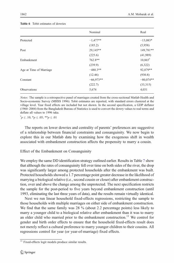
The reports on lower dowries and centrality of parents’ preferences are suggestiveof a relationship between financial constraints and consanguinity. We now begin toexplore this in our Matlab data by examining how the exogenous shift in wealthassociated with embankment construction affects the propensity to marry a cousin.

Effect of the Embankment on Consanguinity

We employ the same DD identification strategy outlined earlier. Results in Table 7 showthat although the rates of consanguinity fell over time on both sides of the river, the dropwas significantly larger among protected households after the embankment was built.Protected households showed a 1.7 percentage point greater decrease in the likelihood ofmarrying a biological relative (i.e., second cousin or closer) after embankment construc-tion, over and above the change among the unprotected. The next specification restrictsthe sample for the post-period to five years beyond embankment construction (until1993, eliminating the last three years of data), and the results remain virtually identical.

Next we run linear household fixed-effects regressions, restricting the sample tothose households with multiple marriages on either side of embankment construction.We find that the same family was 28 % (about 2.2 percentage points) less likely tomarry a younger child to a biological relative after embankment than it was to marryan older child who married prior to the embankment construction.11 We control forgender and birth order effects to ensure that the household fixed-effects result doesnot merely reflect a cultural preference to marry younger children to their cousins. Allregressions control for year (or year-of-marriage) fixed effects.

11 Fixed-effects logit models produce similar results.

Table 6 Tobit estimates of dowries

Nominal Real

Protected −1,477** −13,083*(185.2) (5,958)

Post 29,145** 149,781**

(225.6) (41,989)

Embankment 762.8** 10,865†

(239.9) (6,322)

Age at Time of Marriage −480.3** 92,879**

(12.46) (930.8)

Constant −66,973** −80,074**(222.7) (33,315)

Observations 5,674 4,031

Notes: The sample is a retrospective panel of marriages created from the cross-sectional Matlab Health andSocio-economic Survey (MHSS 1996). Tobit estimates are reported, with standard errors clustered at thevillage level. Year fixed effects are included but not shown. In the second specification, a GDP deflator(1960–2004) from the Bangladesh Bureau of Statistics is used to convert the dowry values to real terms anddeflate all values to 1996 taka.†p ≤ .10; *p ≤ .05; **p ≤ .01


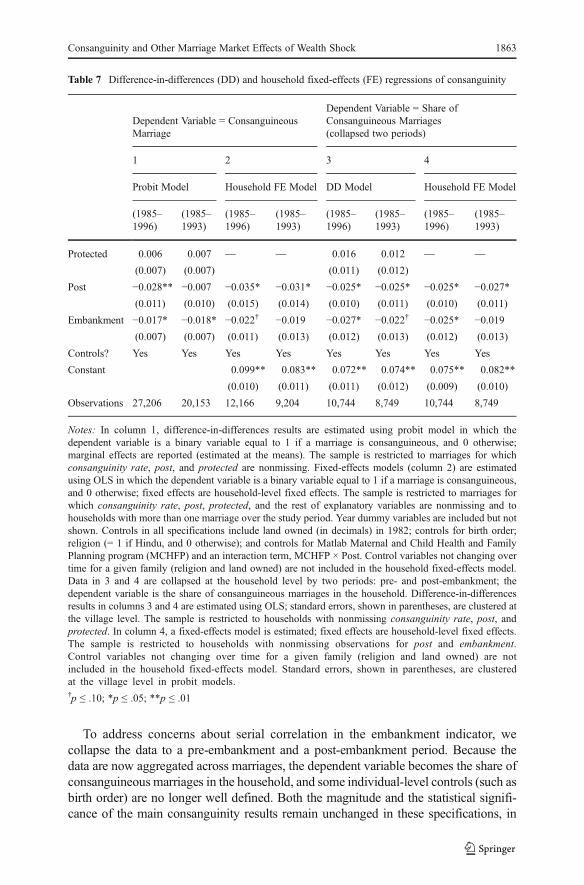
To address concerns about serial correlation in the embankment indicator, wecollapse the data to a pre-embankment and a post-embankment period. Because thedata are now aggregated across marriages, the dependent variable becomes the share ofconsanguineous marriages in the household, and some individual-level controls (such asbirth order) are no longer well defined. Both the magnitude and the statistical signifi-cance of the main consanguinity results remain unchanged in these specifications, in

Table 7 Difference-in-differences (DD) and household fixed-effects (FE) regressions of consanguinity

Dependent Variable = ConsanguineousMarriage

Dependent Variable = Share ofConsanguineous Marriages(collapsed two periods)

1 2 3 4

Probit Model Household FE Model DD Model Household FE Model

(1985–1996)

(1985–1993)

(1985–1996)

(1985–1993)

(1985–1996)

(1985–1993)

(1985–1996)

(1985–1993)

Protected 0.006 0.007 –– –– 0.016 0.012 –– ––

(0.007) (0.007) (0.011) (0.012)

Post −0.028** −0.007 −0.035* −0.031* −0.025* −0.025* −0.025* −0.027*(0.011) (0.010) (0.015) (0.014) (0.010) (0.011) (0.010) (0.011)

Embankment −0.017* −0.018* −0.022† −0.019 −0.027* −0.022† −0.025* −0.019(0.007) (0.007) (0.011) (0.013) (0.012) (0.013) (0.012) (0.013)

Controls? Yes Yes Yes Yes Yes Yes Yes Yes

Constant 0.099** 0.083** 0.072** 0.074** 0.075** 0.082**

(0.010) (0.011) (0.011) (0.012) (0.009) (0.010)

Observations 27,206 20,153 12,166 9,204 10,744 8,749 10,744 8,749

Notes: In column 1, difference-in-differences results are estimated using probit model in which thedependent variable is a binary variable equal to 1 if a marriage is consanguineous, and 0 otherwise;marginal effects are reported (estimated at the means). The sample is restricted to marriages for whichconsanguinity rate, post, and protected are nonmissing. Fixed-effects models (column 2) are estimatedusing OLS in which the dependent variable is a binary variable equal to 1 if a marriage is consanguineous,and 0 otherwise; fixed effects are household-level fixed effects. The sample is restricted to marriages forwhich consanguinity rate, post, protected, and the rest of explanatory variables are nonmissing and tohouseholds with more than one marriage over the study period. Year dummy variables are included but notshown. Controls in all specifications include land owned (in decimals) in 1982; controls for birth order;religion (= 1 if Hindu, and 0 otherwise); and controls for Matlab Maternal and Child Health and FamilyPlanning program (MCHFP) and an interaction term, MCHFP × Post. Control variables not changing overtime for a given family (religion and land owned) are not included in the household fixed-effects model.Data in 3 and 4 are collapsed at the household level by two periods: pre- and post-embankment; thedependent variable is the share of consanguineous marriages in the household. Difference-in-differencesresults in columns 3 and 4 are estimated using OLS; standard errors, shown in parentheses, are clustered atthe village level. The sample is restricted to households with nonmissing consanguinity rate, post, andprotected. In column 4, a fixed-effects model is estimated; fixed effects are household-level fixed effects.The sample is restricted to households with nonmissing observations for post and embankment.Control variables not changing over time for a given family (religion and land owned) are notincluded in the household fixed-effects model. Standard errors, shown in parentheses, are clusteredat the village level in probit models.†p ≤ .10; *p ≤ .05; **p ≤ .01


both DD and household fixed-effects models. In summary, we find robust evidence thata positive wealth shock resulted in a drop in consanguinity.

Is Consanguinity Related to Credit Constraints and Dowries?

The main DD result we have reported is consistent with the Do et al. (forthcoming)hypothesis that dowries and consanguinity act as substitutes in the marriage market. Theembankment, by increasing wealth on the protected side, relaxed the liquidity constraint(in the sense that these now-wealthier households had more dowry to offer at the time ofmarriage), taking away this important motivation for marrying within the family. In thissection, we examine further evidence on a few other implications of this model.

First, we examine the direct correlation between consanguinity and dowries using theretrospective data on dowries from the MHSS 1996 survey. These data indicate that thedowry transfer at the time of marriage is much smaller in consanguineous unions. Theunadjusted bivariate correlation suggests that dowry payments are 25 % lower inconsanguineous marriage. When we control for year fixed effects and other covariatessuch as protection status, the conditional correlation suggests that dowries are 65 %lower at the mean for consanguineous unions. To understand the quantitative signifi-cance (monetary magnitude) of this correlation, we use a GDP deflator from theBangladesh Bureau of Statistics to convert the dowry values to real terms and deflateall values to 1996 taka.We find that consanguinity offers a large quantitatively importantsavings in dowry payment (2,200 taka in nominal terms, or US$276 in 1996 dollars).

The large savings of dowry that consanguinity permits in turn raises the questionwhether the wealth shock associated with the embankment was large enough toenable protected households to substitute away from consanguinity so quickly. The1996 MHSS data indicate that the average farmer on the protected side gainedadditional agricultural profits of 4,300 taka in 1996 because of the extra growingseason, and this had a deflated value of 2,700 in 1987 takas. The wealth effecttherefore does seem large enough to allow the newly protected farmers to use theextra agricultural profits to substitute away from consanguinity. In the MHSS data, anextra 1,300 taka was transferred over in dowries in nonconsanguineous marriages thatwere contracted during the period 1987–1989. Six months of agricultural profits forthe average protected farmer would cover this excess dowry, and the liquidityconstraint preventing households from paying dowries up front thus does get signif-icantly relaxed within the first year.

Because only brides have to pay the dowry, the embankment relaxes a relevantliquidity constraint only for the bride’s family. Table 8 reports the embankment-consanguinity relationship separately for males and females. As predicted by this theory,we observe that the consanguinity effect is stronger in the female sample. Females were2.0–2.9 percentage points less likely to marry consanguineously, an effect that isstatistically significant in every case; the corresponding effect for males was 1.0–1.8percentage points, which is sometimes not significantly different from zero.

The direction of the male-female difference is actually powerful evidence in favor ofthe liquidity constraint story for consanguinity, which helps us distinguish this explana-tion from some other competing models because the leading alternative hypothesis wouldpredict exactly the opposite. We saw in our earlier analysis of dowries that men captured alarger share of the benefits of embankment construction because the marriage market in


rural Bangladesh is patrilocal. Under a simpler story of consanguinity as an inferiormarriage outcome, grooms’ families—not brides’—would experience the larger drop.Furthermore, the symmetry in consanguinity—namely, if a female marries her cousin,then her husband is also marrying his cousin—biases us against finding a significantdifference by gender, which implies that the difference we report is informative.

Consideration of Alternative Hypotheses Linking Consanguinity to the Wealth Shock

We have shown that several patterns in the Matlab data are consistent with a theorylinking consanguinity to credit constraints, but other models may also predict some ofthese same patterns. Ruling out all other theories with full confidence would requireus to specify and estimate a model of the marriage market in which all relevantattributes that are potentially correlated with consanguinity are controlled for, but thisis beyond the scope of these data. In this section, we look for evidence that speaks to afew specific alternative theories.

Table 8 Consanguinity rates in protected households, difference-in-differences estimates

(1982–1996) (1982–1993)

Male Female Male Female

Protected 0.006 0.002 0.014 0.009 0.006 0.003 0.014 0.010

(0.009) (0.009) (0.009) (0.009) (0.009) (0.009) (0.009) (0.009)

Post −0.030* −0.023 −0.017 −0.036* −0.026* −0.017 0.011 −0.037**(0.014) (0.015) (0.010) (0.015) (0.012) (0.015) (0.008) (0.013)

Embankment −0.018† −0.014 −0.027** −0.020* −0.013 −0.010 −0.029** −0.023**(0.010) (0.010) (0.008) (0.008) (0.011) (0.012) (0.008) (0.008)

Land Owned(in Decimals)

−0.000* −0.000 −0.000† −0.000(0.000) (0.000) (0.000) (0.000)

Oldest Child −0.005 0.012** −0.008 0.005

(0.005) (0.004) (0.006) (0.005)

Youngest Child −0.012** 0.013** −0.015** 0.012*

(0.004) (0.004) (0.005) (0.005)

Hindu −0.048** −0.043** −0.044** −0.040**(0.005) (0.005) (0.005) (0.006)

MCHP 0.002 −0.005 0.002 −0.005(0.009) (0.008) (0.009) (0.009)

MCHP × Post 0.010 0.026** 0.011 0.025*

(0.011) (0.010) (0.012) (0.011)

Observations 11,032 11,032 16,174 16,174 8,093 8,093 12,060 12,060

Notes: Difference-in-differences results are estimated using a probit model; marginal effects (estimated atthe mean) are reported. The sample is split by gender and is restricted to marriages for which consanguinityrate, post, protected, and the rest of explanatory variables are nonmissing and to marriages from householdswith more than one marriage during the study period. Year dummy variables are included but not shown.Standard errors, shown in parentheses, are clustered at the village level.†p ≤ .10; *p ≤ .05; **p ≤ .01


There are several other possible conceptual links between the embankment and ratesof consanguinity. First, if consanguinity is a desirable marriage outcome based oncultural or religious preferences, then protected households experiencing a positivewealth shock from the embankment may become more able to attract (or pay for) suchmarriages. This theory is not consistent with our basic DD and fixed-effects resultsshowing differential decreases in consanguinity following embankment constructionrather than increases.

Conversely, if consanguinity is an inferior marriage outcome, protected house-holds—with the additional attractive characteristic they offer on the marriagemarket—may be more likely to avoid this outcome. However, in that case, wewould expect a stronger consanguinity effect in the male sample because thepatrilocal nature of the marriage market means that males would experience adifferentially greater benefit from embankment construction.

A third possibility is that families marry consanguineously to keep wealth andassets within the extended family. Our data indicate that cross-sectionally poorerfamilies were more likely to engage in consanguinity (results available on request),and that following embankment construction, newly wealthy households movedaway from the practice. Both observations directly contradict this hypothesis.

A fourth possibility is that the wealth shock allows protected households to broadentheir search distance over a wider geographical area, which would mechanically lowerconsanguinity if relatives are spatially clustered. To examine this hypothesis, we directlytest whether the embankment construction changed the search distance for protectedhouseholds. Table 9 shows that the embankment had negligible effects on the house-holds’ propensity to marry and relocate farther away.We see no significant effect in eitherthe male or the female sample on marrying into a different village, marrying outside thedistrict, marrying across the river, or the distance to the spouse’s village. Furthermore, thetriple difference result by gender (that the consanguinity effect is larger for females) alsomakes this hypothesis unlikely. Boys’ families initiate the search process in South Asianmarriage markets (Vogl 2011), which implies that the consanguinity-search hypothesiswould result in larger embankment effects in the male sample, unlike what we find.

A fifth theoretical possibility is that consanguinity is a response to risk exposure.Unprotected households may seek mutual insurance by practicing consanguinity as a wayto form robust intergenerational bonds with another household in the extended family.However, the discussion and results presented earlier suggest that the embankmentprimarily acted as a wealth shock rather than mitigating risk. Moreover, the results inTable 9 suggest that other marriage outcomes associated with risk are unchanged follow-ing embankment construction. For example, the model in Online Resource 1 suggests thatif the embankment mitigates flood risk, we should observe negative assortative matchingwith respect to protection status. The coefficient on Protected in Specification 3 of Table 9shows that households are, in general, much more likely to marry others who are locatedcloser to them—an indication of search frictions in the marriage market—but thispropensity to marry close does not differentially change after embankment construction.12

12 This highlights the possibility that empirical results on assortative matching based on cross-sectional datamay be uninformative because separating search frictions from true assortative matching in cross-sectionaldata is difficult. Our panel data, which allow us to control for both “protected” and “post × protected”(labeled “embankment”) helps resolve the issue.


For risk-averse households, embankment protection may lower their demand for mitigat-ing risk through other channels (e.g., marrying daughters into geographically distanthouseholds that are not subject to the same weather patterns or planting different crops,à la Rosenzweig and Stark 1989). We would then expect to see changes in femalemigration patterns for marriage following embankment construction. Table 9 shows no

Table 9 Probit estimates of spouse search hypothesis

1 2 3 4

Spouse From aDifferent Village

Spouse FromOutside of Matlab

Marriage Acrossthe River

Distance to Spouse’sVillage (OLS)

Male Female Male Female Male Female Male Female

Protected −0.013 −0.010 −0.151** −0.053 0.183** 0.108 0.089 −0.129(0.015) (0.013) (0.024) (0.033) (0.036) (0.093) (0.189) (0.278)

Post 0.029 0.000 0.033 −0.001 0.024 0.009 0.572* 0.060

(0.020) (0.013) (0.029) (0.022) (0.033) (0.036) (0.248) (0.233)

Embankment −0.002 −0.002 0.034 −0.009 −0.023 0.020 −0.250 −0.032(0.011) (0.011) (0.022) (0.015) (0.023) (0.021) (0.162) (0.161)

Land Owned(in decimals)

0.000 0.000** 0.001* 0.001** 0.000 0.001 0.004† 0.006*

(0.000) (0.000) (0.000) (0.000) (0.000) (0.000) (0.002) (0.003)

Oldest Child 0.004 −0.023** −0.007 −0.011 0.007 −0.011 −0.075 −0.283**(0.006) (0.006) (0.013) (0.008) (0.013) (0.011) (0.094) (0.089)

Youngest Child 0.039** −0.010* 0.019* −0.001 0.014 −0.023* 0.352** −0.103(0.007) (0.005) (0.009) (0.008) (0.012) (0.011) (0.078) (0.069)

Hindu 0.014 0.002 0.019 −0.043† 0.058† 0.028 0.864* 1.112**

(0.028) (0.023) (0.020) (0.022) (0.031) (0.031) (0.351) (0.353)

MCHP −0.014 0.000 0.007 0.033 −0.078* −0.095* −0.193 −0.291(0.015) (0.011) (0.023) (0.022) (0.032) (0.040) (0.206) (0.213)

MCHP × Post 0.012 0.004 0.004 −0.000 −0.008 −0.016 −0.217 −0.068(0.010) (0.010) (0.020) (0.016) (0.023) (0.022) (0.163) (0.161)

Constant 2.470** 3.182**

(0.230) (0.245)

Observations 12,924 20,023 12,924 20,023 6,161 7,170 6,497 7,628

Notes: Estimates from the probit models are presented in columns 1–3, where the dependent variable is abinary variable equal to 1 if a spouse is from a different village, and 0 otherwise (column 1); a binaryvariable equal to 1 if a spouse is from outside of Matlab, and 0 otherwise (column 2); a binary variableequal to 1 if a marriage is across the embankment, and 0 otherwise (column 3); a binary variable equalto 1 if a marriage is consanguineous and at least one spouse is not from outside Matlab, and 0 otherwise(column 3). Marginal effects are reported (estimated at the means); the sample is split by gender. In 4,estimates are from the OLS model in which the dependent variable is the distance (in km) between thespouses’ villages within Matlab. In columns 3 and 4 the sample is restricted to marriages within Matlab(where consanguinity status is nonmissing). Year dummy variables are included but not shown. Standarderrors, shown in parentheses, are clustered at the village level.†p ≤ .10; *p ≤ .05; **p ≤ .01


evidence of such behavior: neither girls nor boys were more likely to marryfarther away. Increasing wealth may also alter household tastes for risk, but wedo not find much evidence either from our fieldwork or in the data that theembankment changed households’ risk exposure or their propensity to diversifyand hedge against risk through marriage.

Although we report a congruent set of results that jointly amount to strongsuggestive evidence that dowries and credit constraints are linked to the practice ofconsanguinity, there are other plausible explanations for some of our results that aredifficult to rule out. The joint distribution of consanguinity with other characteristicsthat matter in the marriage market may lead to incidental correlations among con-sanguinity, wealth, and gender. For example, if grooms care about an unmeasuredcharacteristic (such as beauty) but brides care about status, and status is similar withinconsanguineous groups but not beauty, then the wealth shock may lead to a drop inconsanguinity among brides but not grooms. Absent data on all relevant characteris-tics in the marriage market (some of which, like beauty, are not easily measurable), itis impossible to confidently rule out these alternative hypotheses.

Additional Sensitivity Analysis

Table S3 in Online Resource 1 reports a battery of sensitivity checks on our mainresults. One concern with our results is that the unprotected side is twice as large inarea and population than the protected side. This means that unprotected householdsare, on average, farther from the river and therefore, on average, are not comparablewith protected households. We omit the households farthest from the river either onlyon the unprotected side or on both sides, and show that the main consanguinity effectthat we report in this article is unchanged.

Next, we check that our results are not generated by the endogenous sorting ofhouseholds around the embankment after construction. Five percent of our samplemigrate to another area in Matlab during the post-embankment period for a reason otherthanmarriage, and reestimating the models without these migrants does not qualitativelychange the results.13 In addition, our results are robust to the exclusion of non-Muslims,who follow different marriage customs and face a narrower market. The main resultsalso hold if we control for religion, which is important because the fraction of thepopulation that is Hindu was different at baseline across the two banks of the river.

We also conduct falsification exercises on our DD estimates (modeled after Aghion etal. 2008), which replace the indicator for the actual year of embankment constructionwith every other possible false embankment year of the sample. In other tests, we replacethe variable for protection status (indicating which side of the embankment a householdis on) with false embankment locations of northern versus southern villages and thetreatment and control groups of the Matlab Maternal and Child Health and FamilyPlanning (MCHFP) Program, an experimental program present in the area. These testsfor false times and locations all show that statistical impacts are absent in cases where weshould not observe them (e.g., we see no statistical differences in behavior across anytwo subperiods other than that of embankment construction) and that the actual

13 Strong and Minkin (1992) also analyzed migration data before and after construction and concluded thatthere are no real changes in out-migration rates for either the protected or the unprotected areas.


embankment effect typically trumps the false embankment effects.14 The main consan-guinity effect also survives when a direct control is added for the MCHFP.

Conclusion

With the high prevalence of consanguinity in South Asia, the Middle East, and NorthAfrica, it is important to understand the underlying socioeconomic drivers of thispractice. Data from rural Bangladesh are consistent with a hypothesis that poorhouseholds engage in consanguinity partly in response to their inability to paydowries up front at the time of marriage. This helps to explain why a large populationgenetics literature has found that people of lower SES are most likely to engage inconsanguinity. If the credit-constraint explanation is correct, then the high childmorbidity and mortality effects of consanguinity reported in the literature imply thatliquidity constraints and lack of access to credit impose yet another costly burden onpoor households in developing countries through their marriage market choices.

This article also documents further changes in marriage markets following wealthgains that accrue to a subset of Matlab residents. Despite a long literature on theconsequences of assortative mating for inequality in developed countries, fewer studieshave documented these patterns in developing countries (Esteve andMcCaa 2008;Mare1991). The marriage market is increasingly segregated in terms of spousal wealth.Members of farming households who benefit from the wealth shock are differentiallymore likely to marry into wealthy households, and nonfarmers living on the protectedside of the river find it increasingly difficult to marry into the now-wealthier farminghouseholds. Men from these protected (wealthier) households start commanding largerdowries. However, norms regarding age at marriage appear much more inelasticcompared with the quicker changes in spousal SES that we document.

Finally, our article documents the general equilibrium changes associated with aninfrastructure project in disaster mitigation. Evaluations of such projects typicallyfocus on direct impacts on ecosystem equilibrium, agricultural practices and incomes,and health (e.g., Haque and Zaman 1993; Myaux et al. 1997; Paul 1995; Thompsonand Sultana 1996), and we show that indirect general equilibrium changes can bequite substantial and need to be taken into account in program evaluation.

Acknowledgments We thank the National Science Foundation Human and Social Dynamics Grant SES-0527751 for financial support; ICDDR,B for their hospitality during fieldwork; and Andrew Foster, GrantMiller, Murat Iyigun, Aloysius Siow, Mark Rosenzweig, Eric Edmonds, Paul Schultz, and seminarparticipants at the University of California-Berkeley, Boston College, University of Maryland–CollegePark, University of Washington at Seattle, the University of British Columbia, Penn State, Yale School ofManagement, University of Colorado at Boulder (IBS), 9th BREAD Conference, and the EconometricSociety meetings for helpful comments and discussion.

14 The t statistic for the actual program coefficient is greater than the t statistic for any false program in100 % of specifications for consanguinity and 92 % of specifications for marrying a wealthy spouse (i.e.,one owning an above average amount of land). When the actual and false program groups are both includedin the same regression, the actual program coefficient is significant at the 10 % level in 100 % ofspecifications for consanguinity and in 54 % of specifications for marrying a wealthy spouse. The falseprogram coefficient is significant in only 20 % of consanguinity specifications and is never significant formarrying a wealthy spouse.


References

Aghion, P., Burgess, R., Redding, S., & Zilibotti, F. (2008). The unequal effects of liberalization: Evidencefrom dismantling the License Raj in India. American Economic Review, 98, 1397–1412.

Ambrus, A., Field, E., & Torero, M. (2010). Muslim family law, prenuptial agreements and the emergenceof dowry in Bangladesh. Quarterly Journal of Economics, 125, 1349–1397.

Amin, S., & Cain, M. (1997). The rise of dowry in Bangladesh. In G. W. Jones, R. M. Douglas, J. C.Caldwell, & R. M. D’Souza (Eds.), The continuing demographic transition (pp. 290–306). Oxford,UK: Clarendon Press.

Anderson, S. (2007). Why the marriage squeeze cannot cause dowry inflation. Journal of EconomicTheory, 137, 140–152.

Banerjee, A., Duflo, E., Ghatak, M., & Lafortune, J. (2009). Marry for what? Caste and mate selection inmodern India (NBER Working Paper No. 14958). Cambridge, MA: National Bureau of EconomicResearch.

Becker, G. S. (1973). A theory of marriage: Part I. Journal of Political Economy, 81, 813–846.Becker, G. (1991). Treatise on the family. Cambridge, MA: Harvard University Press.Bertrand, M., Duflo, E., & Mullainathan, S. (2004). How much should we trust differences-in-differences

estimates? Quarterly Journal of Economics, 119, 249–275.Bittles, A. H. (1994). The role and significance of consanguinity as a demographic variable. Population and

Development Review, 20, 561–584.Bittles, A. H. (2001). Consanguinity and its relevance to clinical genetics. Clinical Genetics, 60, 89–98.Bittles, A. H., & Makov, U. (1988). Inbreeding in human populations: Assessment of the costs. In C. Mascie-

Taylor & A. Boyce (Eds.),Mating patterns (pp. 153–167). Cambridge, UK: Cambridge University Press.Bittles, A. H., & Neel, J. V. (1994). The costs of human inbreeding and their implications for variations at

the DNA level. Nature Genetics, 8, 117–121.Bloch, F., & Rao, V. (2002). Terror as a bargaining instrument: A case study of dowry violence in rural

India. American Economic Review, 92, 1029–1043.Botticini, M., & Siow, A. (2003). Why dowries? American Economic Review, 93, 1385–1398.Briscoe, J. (1998). Against the flow: Reflections on two decades of development in a Bangladeshi village.

Unpublished manuscript, The World Bank, Washington, DC.Caldwell, J., Reddy, P., & Caldwell, P. (1983). Causes of marriage change in south India. Population

Studies, 37, 343–361.Deininger, K., Goyal, A., & Nagarajan, H. (2010). Inheritance law reform and women’s access to capital:

Evidence from India’s Hindu Succession Act (World Bank Policy Research Working Paper 5338).Washington, DC: World Bank.

Do, Q.-T., Iyer, S., Joshi, S. (Forthcoming). The economics of consanguineous marriages. The Review ofEconomics and Statistics.

Edlund, L. (1999). Son preference, sex ratios, and marriage patterns. Journal of Political Economy,107, 1275–1304.

Esteve, A., & McCaa, R. (2008, September). Assortative mating patterns in the developing world. Paperpresented at the 2009 IUSSP Seminar on Changing Transitions to Marriage, New Delhi, India.

Fafchamps, M., & Quisumbing, A. (2005). Assets at marriage in rural Ethiopia. Journal of DevelopmentEconomics, 77, 1–25.

Field, E., & Ambrus, A. (2008). Early marriage, age of menarche, and female schooling attainment inBangladesh. Journal of Political Economy, 116, 881–930.

Givens, B. P., & Hirschman, C. (1994). Modernization and consanguineous marriage in Iran. Journal ofMarriage and the Family, 56, 820–834.

Goode, W. J. (1963). World revolution and family patterns. New York: Free Press.Gould, E. D., Moav, O., & Simhon, A. (2008). The mystery of monogamy. American Economic

Review, 98, 333–357.Grant, J. C., & Bittles, A. H. (1997). The comparative role of consanguinity in infant and childhood

mortality in Pakistan. Annals of Human Genetics, 61, 143–149.Han, H. (2010). Trends in educational assortative marriage in China from 1970 to 2000. Demographic

Research, 22(article 24), 733–770. doi:10.4054/DemRes.2010.22.24Haque, C., & Zaman, M. (1993). Human responses to riverine hazards in Bangladesh: A proposal for

sustainable floodplain development. World Development, 21, 93–107.Hitsch, G., Hortacsu, A., & Ariely, D. (2010). Matching and sorting in online dating. American Economic

Review, 100, 130–163.


http://dx.doi.org/10.4054/DemRes.2010.22.24

Jacoby, H. G. (1995). The economics of polygyny in sub-Saharan Africa: Female productivity and thedemand for wives in Côte d'Ivoire. Journal of Political Economy, 103, 938–971.

Jacoby, H. G., & Mansuri, G. (2010). Watta satta: Bride exchange and women’s welfare in rural Pakistan.American Economic Review, 100, 1804–1825.

Jahan, R. (1990). Hidden wounds, visible scars: Violence against women in Bangladesh. In B. Agarwal(Ed.), Structures of patriarchy: State, community and household in modernising Asia (pp. 199–227).London, UK: Zed Books.

Jensen, R., & Thornton, R. (2003). Early female marriage in the developing world. Gender andDevelopment, 11(2), 9–19.

Kabir, M. (2004). Development or a disaster forgotten? The case of Meghna-Dhonagoda Irrigation andFlood Control Project (Working paper). Dhaka: ActionAid Bangladesh.

Mare, R. D. (1991). Five decades of educational assortative mating. American Sociological Review, 56, 15–32.Mensch, B. S., Singh, S., & Casterline, J. B. (2005). Trends in the timing of first marriage among men and

women in the developing world. In C. B. Lloyd, J. R. Behrman, N. P. Stromquist, & B. Cohen (Eds.),The changing transitions to adulthood in developing countries: Selected studies (pp. 118–171).Washington, DC: The National Academies Press.

Mobarak, A. M., Chaudhry, T., Brown, J., Zelenska, T., Bittles, A. H., Khan, N., . . . Rana, A. W. (2012).Doesmarrying your cousin affect your child? Using a unique IV approach to measure the effects of consan-guinity on child health outcomes. Unpublished manuscript, School of Management, Yale University.

Myaux, J. A., Ali, M., Chakraborty, J., & de Francisco, A. (1997). Flood control embankments contributeto the improvement of the health status of children in rural Bangladesh. Bulletin of the World HealthOrganization, 75, 533–539.

New York Times. (2003, September 28). The struggle for Iraq: Traditions; Iraqi family ties complicateAmerican efforts for change. Retrieved from www.nytimes.com

Paul, B. (1995). Farmers’ responses to the Flood Action Plan (FAP) of Bangladesh: An empirical study.World Development, 23, 299–309.

Protik, A., & Kuhn, R. (2006). The hidden cost of migration: Effect of brother’s migration on sister’s marriageoutcomes in rural Bangladesh. Unpublished manuscript, Department of Economics, Brown University.

Rahman, O., Menken, J., Foster, A., & Gertler, P. (1996). Matlab [Bangladesh] Health and SocioeconomicSurvey (MHSS), 1996 [Computer file]. 5th ICPSR version. Santa Monica, CA: RAND [producer], 2001.Ann Arbor, MI: Inter-university Consortium for Political and Social Research [distributor], 2001.

Rao, V. (1993). The rising price of husbands: A hedonic analysis of dowry increases in rural India. Journalof Political Economy, 101, 666–677.

Rosenzweig, M. R., & Stark, O. (1989). Consumption smoothing, migration, and marriage: Evidence fromrural India. Journal of Political Economy, 97, 905–926.

Rowlatt, J. (2005, November 16). The risks of cousin marriage. BBC Newsnight. Retrieved fromwww.news.bbc.co.uk

Sandridge, A. L., Takeddin, J., Al-Kaabi, E., & Frances, Y. (2010). Consanguinity in Qatar:Knowledge, attitude and practice in a population born between 1946 and 1991. Journal ofBiosocial Science, 42, 59–82.

Shah, G., Toney, M., & Pitcher, B. (1998). Consanguinity and child mortality: The risk faced by families.Population Research and Policy Review, 17, 275–283.

Siow, A. (1998). Differential fecundity, markets and gender roles. Journal of Political Economy, 106, 334–354.Strong, M. A., & Minkin, S. F. (1992). The demographic, health, and nutritional impacts of the Meghna-

Dhonagoda embankment (Bangladesh Flood Action Plan FAP 16 Environmental Study, SpecialStudies Program). Dhaka, Bangladesh, and Arlington, VA: ICDDR,B and ISPAN.

Thompson, P. M., & Sultana, P. (1996). Distributional and social impacts of flood control in Bangladesh.The Geographical Journal, 162, 1–13.

Tiemoko, R. (2001). The gender age gap: Marriage and rights in the Cote d’Ivoire.Development, 44, 104–106.Vogl, T. (2011). Sisters, schooling, and spousal search: Evidence from South Asia (Working paper).

Department of Economics and Woodrow Wilson School. Princeton, NJ: Princeton University.Weiss, Y. (1997). The formation and dissolution of families: Why marry? Who marries whom? And what

happens upon divorce. In M. Rosenzweig & O. Stark (Eds.), Handbook of population and familyeconomics (pp. 81–124). Amsterdam, Netherlands: Elsevier Science.

Wickrama, K. A. S., & Lorenz, F. O. (2002). Women’s status, fertility decline, and women’s health in developingcountries: Direct and indirect influences of social status on health. Rural Sociology, 67, 255–277.

Wong, Y. Y. (2003). Structural estimation of marriage models. Journal of Labor Economics, 21, 699–728.Zlotogora, J. (2002). What is the birth defect risk associated with consanguineous marriage? American

Journal of Medical Genetics, 109, 70–71.


http://www.nytimes.com

http://www.news.bbc.co.uk

consanguinity and other marriage market effects of a ...€¦ · consanguinity and other marriage...

Documents