Happy Hens, sad consumers? The Economic Impact of Restrictions on Farm Animal Housing in California

Conner Mullally1 and Jayson L. Lusk

This version: November 13, 2015 New animal welfare policies on the horizon in many states have prompted debates about the cost of achieving happier hens and hogs. A recent policy change in California offers a unique opportunity to measure the economic repercussions of minimum space requirements for egg-laying hens. Using retail scanner data from large California and non-California markets, we use difference-in-difference estimators to identify the effect of minimum space requirements on retail egg prices, quantity sold, and sales value, while also estimating impacts of the policy change on consumer welfare and egg producer net revenue. We estimate that the law increased egg prices by about 22%, decreased quantity sold by around 8%, and increased the value of sales by about 12%; the price and sales effects are statistically significant at conventional levels. In the three California markets included in our data set, consumer welfare losses amount to approximately $30 million over the 16 weeks immediately following implementation of minimum space requirements while net revenue from eggs sold in the three California markets increased by between 11% and 15% over the same time horizon. Positive impacts on producers may have been short lived, however, and were likely concentrated among producers located in California. Our results are robust to several tests of our identifying assumptions. Overall, our findings indicate that the potential economic costs of mandated improvements in farm animal welfare should be taken seriously when considering such policy changes. JEL Codes: C54, D04, Q18

1 Corresponding author: PO Box 110240 Gainesville, FL 32611-0240 (352) 294-7680 connerm@ufl.edu

1

There are more egg-laying chickens in the United States than there are people. Until

recently, virtually all of those hens live in so-called battery cages that provide an amount

of space per hen that is 28% smaller than a typical 8.5 by 11 inch sheet of paper. On January

1, 2015, two new laws motived at least in part by the goal of improving animal welfare

(henceforth referred to as the AW laws) went into place requiring that all eggs sold in

California come from chickens provided enough room to turn around and fully extend their

wings.2 Other states will soon implement similar measures, and additional federal and state

laws are being actively debated.3 In addition, Wal-Mart has encouraged its food suppliers

to adopt more humane housing standards for farm animals, and McDonald’s has pledged

to phase out the use of eggs produced by hens living in battery cages (Polansek and Nickel

2015, Nassauer 2015). Momentum for more widespread adoption of more animal-friendly

housing standards appears to be growing in the private sector and the legislative arena alike,

raising questions about the potential economic costs of such restrictions.

2 California voters passed Proposition 2 in 2008 banning confinement of farm animals that does not allow them to turn around freely, lie down, stand up, and fully extend their limbs. The measure applied to chicken battery cages, veal crates, and sow gestation crates. However, there is very little veal, pork, or broiler production in California, while California is the 7th largest egg producing state in the nation (producing 4.5 billion eggs in 2014 or 5.1% of the nation’s total according to USDA-NASS). Therefore the potential impacts are largest for the egg industry. In addition, recognizing that cheaper imports from other states would soon dominate the egg market, the California state legislature passed AB 1437 in 2010, banning the sale of eggs in California produced under conditions that do not comply with Proposition 2. Both laws were implemented on January 1, 2015. 3 Four other states (Michigan, Ohio, Oregon, and Washington) have already passed laws that will eventually limit the use of battery cages. Similar measures are being considered in many other locales (e.g., Massachusetts has a voter initiative on the ballot in November 2015 that would prohibit the production and sale of eggs using batter cages). In 2012, two common foes, the Humane Society for the United States (HSUS) and the United Egg Producers (UEP) jointly lobbied the US Congress (unsuccessfully) for a federal law that would have required a minimum space per hen. The agreement fell apart when the Farm Bill passed in 2014 without the standards. All of these efforts follow European Union laws that banned battery cages in 2012.

2

US consumers eat around 250 eggs per person per year on average (USDA-ERS

2015), and as a result housing restrictions for egg-laying hens have the potential to burden

consumers with higher food costs. The issue of cost is also at the crux of a paradox

surrounding consumer behavior. When California voters went to the polls in 2008 and

passed the initiative mandating minimum space requirements for farm animals that would

eventually be implemented in 2015, about 90% of California consumers were buying

battery cage eggs despite the existence of many alternative, albeit more expensive, options

(Chang, Lusk and Norwood 2010). The fact that most consumers were unwilling to pay the

higher price of the non-cage alternatives in the grocery store led Allender and Richards

(2010) to project over $100 million in consumer welfare losses as a result of the policy.

Because egg demand is relatively inelastic (Brown and Schrader 1990, Okrent and Alston

2011) and the product has few close substitutes, small changes in cost could translate into

large price increases, disproportionately impacting low-income consumers (Allender and

Richards 2010).

Aside from consumer welfare concerns, others have also suggested California egg

producers will suffer economic losses (Sumner et al. 2011). California is a net importer of

eggs, and as a result, concern over impacts on egg producers extends beyond California’s

borders. Seven other states sued the state of California over the prohibition against the sale

3

of eggs not meeting the standards of the AW laws, arguing that the AW laws violate the

Interstate Commerce Clause and harm producers in their states.4

This paper aims to identify the causal impact of the California AW laws on market

outcomes (price, quantity sold, and value of sales) in the California retail egg market as

well as impacts on the welfare of California consumers and producers of eggs sold in

California. Using a difference-in-differences approach applied to retail scanner data from

three major California markets and three non-California markets for weeks observed before

and after January 1, 2015, we estimate that the AW laws increased the average price per

dozen eggs by about 22% relative to what the average price per dozen eggs would have

been had the AW laws not been implemented. We use estimated price impacts to

approximate the equivalent variation of the AW laws for the three California markets in

our data. We find that over the 16 weeks following implementation of the AW laws that

we observe in our data set, consumers in the three selected California markets would have

been willing to pay about $30 million dollars to avoid the price changes caused by the AW

laws. Extrapolating this figure out to an annual figure for California as a whole yields a

total annual willingness to pay to avoid the price increases caused by the AW laws of $105

million.

In addition, we estimate that the AW laws caused the quantity of eggs sold to fall

by about 7.9% relative to what would have been observed had the AW laws not been

4 A federal court judge dismissed the case in 2014, but the dismissal is currently under appeal.

4

implemented; however, we cannot reject the null hypothesis of zero effect on quantity sold.

We find evidence that supply responses to the AW laws vary by producer location, and that

California producers appear to be increasing supply in response to the AW laws while out-

of-state producers are reducing supply. Estimated sales impacts indicate that the AW laws

lead to an 11.8% increase in the value of egg retail sales in the three California markets.

By combining our data with assumptions about the impact of the AW laws on producer

costs and the producer share of the retail egg price, we estimate that the AW laws increased

net producer revenue by between 11% and 15% over the 16 post-implementation weeks

observed in our data; however, nearly all of the increase in net revenue appears to have

been driven by the initial price surge associated with implementation of the AW laws.

Given the fact that minimum space requirements for hen housing or outright bans

on battery cages may ultimately become policy in other states, the issue has been studied

in a number of prior papers. However, nearly all previous efforts to address this issue are

ex-ante analyses, relying on simulation models (Sumner, Matthews, et al. 2010; Norwood

and Lusk 2011; Allender and Richards 2010), budgetary comparisons of cage and cage-

free systems (Matthews and Sumner 2015; Sumner, et al. 2008), or hedonic analyses of

retail egg prices (Chang, Lusk and Norwood 2010). While each of these approaches

provided useful insights, none provide an ex-post analysis of the actual policy that may

ultimately become law elsewhere. Other than the present paper, the only other ex-post

analysis of the California AW laws of which we are aware is Malone and Lusk (2015), who

rely on (potentially non-representative) reports of wholesale prices to the USDA

5

Agricultural Marketing Service rather than retail prices, do not have access to quantity or

sales data, and do not estimate producer welfare impacts.

Our paper makes a number of significant contributions over previous related work.

As far as we know, our paper is the first to provide an ex-post estimate of the impact of

farm animal housing restrictions on retail prices, quantities, and sales, as well as effects on

producer and consumer welfare. This paper contributes to the relatively nascent literature

on the economics of animal welfare (Cowen 2006, Lusk and Norwood 2011). Some animal

welfare advocates suggest such policies are inexpensive (costing less than an extra penny

per egg) ways to improve animal well-being (Hall 2008). Some animal advocates have

even suggested that laws eliminating tight confinement might raise producer profits based

on the premise that current conditions are so inhospitable that they lower productivity

(Francione and Garner 2010). Aside from productivity effects, such laws might also

increase producer profits by reducing the volume of eggs supplied. Indeed, several food

retailers have sued large egg producers and their industry organization over allegations of

artificial supply constraints enacted, in part, by increasing cage size limits (Harris 2011).

Perhaps surprisingly, some animal rights advocates have argued against policies like the

California law that improve the well-being of farm animals because such policies may

increase consumer demand, leading to greater consumption of animal products (Francione

2008). Our unique data on prices and quantities at the retail level can help provide insights

into such debates.

In what follows, we first summarize the data set used in our analysis, and then

describe our identification strategy. We then present our estimated impacts on market

6

outcomes before moving onto our analysis of impacts on consumer and egg producer

welfare. Next, we subject our results to robustness checks, estimating placebo impacts on

non-California markets and checking the robustness of our results to violations of the

common trends assumption underlying difference-in-differences estimation. We end with

a brief conclusion.

Data

To conduct our analysis, we use retail scanner data from Nielsen for three California

markets (Los Angeles, San Francisco, and San Diego) and three non-California markets

(Chicago, Phoenix, and Salt Lake City/Boise). The data set was constructed by aggregating

weekly reports from participating retailers. Nationally, Nielsen scanner data include

retailers that account for 90% of all grocery sales volume. The geographic scope of each

Nielsen market includes the metropolitan area associated with the market name along with

surrounding counties. Total population in the three California markets is about 28.5 million

(9.6 million households), or 73% of California’s total population, while total population in

the three control markets is about 15.7 million (7.3 million households). The three

California markets were chosen in order to create a data set that is broadly representative

of major metropolitan areas in California, while the non-California markets were chosen

in order to construct a comparison group that included two moderately sized markets and

one large market, yielding a population distribution similar to that of the three California

markets; Los Angeles accounts for 62% of total population in the three California markets,

while Chicago accounts for 58% of total population in the three control markets.

7

The data set runs from the first week of April 2013 through the third week of April

2015; the first 89 weeks of data fall immediately prior to implementation of the AW laws,

while the final 16 weeks cover the period immediately afterward. The data set consists of

142,170 weekly observations of 798 egg Universal Product Codes (UPC), where a single

UPC sold in two different markets during the same week is treated as two separate

observations. The data only include shell eggs (liquid eggs, which are used predominantly

by the food processing and food services industries, are not included in the data set).

Sumner et al. (2008) estimate that about 93% of all eggs produced in California are sold as

shell eggs. Each observation includes average price, units sold, and product characteristics

(package size, grade, cage free or organic certification, etc.) for a UPC in a given market

and week. All UPCs are observed over the entire time horizon covered by the data set.

[TABLE 1 HERE]

Table 1 contains summary statistics calculated using the 89 weeks of data available

prior to implementation of the AW laws. Panel A of table 1 gives the average price per

dozen, average quantity sold per week (in thousands of dozens), and average weekly sales

(in $100,000) in the selected California and non-California markets for weeks in the data

prior to the implementation of the AW laws; prices and sales are in nominal dollars.

Average price was estimated by weighting each UPC’s weekly price by its share of quantity

sold in that week and summing the share-weighted prices. Prices and quantities are higher

in California than in control markets for the pre-implementation period, and the differences

are significant; this is expected, given the differences in market size and the large number

of observations in the data.

8

Panel B of table 1 gives the quantity-weighted average characteristics of eggs sold

in California and non-California markets. Product characteristics are very similar across

the two groups of markets. In general, any significant differences we observe are small in

magnitude. Conventional and white eggs dominate sales volume, with organic and cage-

free eggs each accounting for less than 10% of total sales volume (organic and cage-free

are not mutually exclusive categories). A total of 466 UPCs are sold in the selected

California markets, and 512 are sold in the three non-California markets; 180 UPCs are

sold in both sets of markets.

Empirical approach

Identification and inference

We are interested in estimating the effect of the AW laws on market outcomes as well as

consumer and producer welfare. In order to estimate impacts on market outcomes, we

estimate the following two regression models for each outcome:

(1) 0 1 2 3 4imt m t m t im imty CA Post CA Post x eβ β β β β= + + + × + +

(2) 1imt i m t m t imty CA Post uλ λ λ α= + + + × +

The outcome variable, imty , is average price per dozen, quantity sold, or total sales

for UPC i when sold in market m in week t; mCA is a dummy variable equal to one for

markets within California and zero otherwise; tPost is a dummy variable equal to one for

all weeks following the implementation of the AW laws; imx is a vector of product

characteristics and their interactions; iλ , mλ , and tλ are fixed effects for UPC, market, and

9

week, and imte and imtu are error terms, each of which is assumed to have a mean of zero

conditional on the variables in their respective models. In equation (1), 3β represents the

policy effect in a simple difference-in-differences model augmented to include product

characteristics, while 1α in equation (2) represents the policy effect in a difference-in-

differences model that replaces imx , mCA , and tPost with fixed effects for UPC, market,

and week.

When using average price per dozen as the dependent variable, equations (1) and

(2) are estimated by weighted least squares, where the weight for a particular UPC-market-

week observation is given by total dozens sold by that UPC in the same market and week.

This weighting scheme ensures that in our price regressions, 3β and 1α are estimators of

the impact of the AW laws on the average price per dozen in California, rather than average

impacts per UPC. For our quantity and sales models, our estimates of 3β and 1α are scaled

up by the number of UPCs sold in California in order to convert UPC-level impacts into

impacts on dozens of eggs sold and total egg sales for the three California markets in our

data. Statistical inference is based on two-way cluster-robust standard errors that cluster on

UPC and week (Cameron, Gelbach and Miller 2011), and p-values generated by a wild

cluster bootstrap percentile-t procedure clustering on market.56 Each method of inference

5 Alternatively, we could have treated California as a single cluster. However, to our knowledge, there are no accurate methods of performing statistical inference on the effect of a discrete policy change affecting a single cluster when the number of control clusters is small. Therefore we opt to treat each of the California markets as a single cluster. 6 Theory and simulation evidence in MacKinnon and Webb (2015) and Webb (2014) suggests that the wild cluster bootstrap method used in our paper is likely to reject a true null hypothesis less frequently than what

10

is appropriate under different, but equally reasonable, assumptions about the correlation of

regression error terms across observations; we include both as a check on the robustness of

our results.

Difference-in-differences will yield unbiased estimates of the impact of the AW

laws on market outcomes in California if three assumptions hold: first, that there were no

spillover effects on other states in our data, second, that the three California markets and

the three non-California markets in our data set would have followed the same trends with

respect to price, quantity, an sales in the absence of the AW laws, and third, that there were

no effects of the AW laws prior to its implementation.

California is a net importer of eggs, making it possible that new regulations in

California could affect egg prices elsewhere in the U.S. However, California imports

constitute around 2.4% of total U.S. consumption of eggs, making it unlikely in our view

that a shock to supply or demand in California would reverberate throughout egg markets

elsewhere (Bell 2013, Promar International 2009); therefore we assume that the assumption

of no spillovers holds in the present case. We examine the visual evidence for the

assumptions of common trends in California and non-California markets and no pre-

implementation effects of the AW laws in figure 1.

[FIGURE 1 HERE]

is dictated by the chosen significance level when the number of clusters experiencing a policy change is small. Our own simulation evidence suggests that the wild cluster bootstrap procedure is likely to under reject the null hypothesis in the present context as well, i.e., our p-values may be too large. Our simulation results and additional details on our inference procedures are available in the appendix.

11

The top panel of figure 1 depicts the weekly quantity-weighted average price per

dozen for the three California markets and the three non-California markets. The line

emanating from the horizontal axis at January 2015 represents the implementation of the

AW laws. The two sets of markets are clearly following similar trends until eight weeks

prior to the implementation of the AW laws at which point prices in California begin to

climb sharply. The average price per dozen reaches a peak of $4.09 in February 2015 before

falling back to $2.99 per dozen at the end of April, leaving the price per dozen eggs $0.50

higher at the end of the observed period than the average price before the implementation

of the AW laws and $0.42 higher than the average price per dozen immediately prior to the

sharp increase in prices shown in the figure.

The middle panel of figure 1 shows total dozens sold each week for California and

non-California markets in the data set. Again, we see similar trends evolving in California

and non-California markets, although the co-movement is not as clear as in the case of

prices. Total dozens sold in the three California markets begins to fall relative to sales in

the three control markets at around the same time we observe the structural break in prices

in the top panel. Finally, the bottom panel of figure 1 shows trends for total value of retail

sales of eggs in the three California and non-California markets. The vertical distance

between the two trends is slightly larger in 2014 than in 2013, but overall, the two trends

track each other very closely, exhibiting similar seasonal fluctuations (with upticks in sales

from November through January and again in March and April). As in the case of prices,

we see what appears to be a structural break in the California trend just prior to

implementation of the AW laws, although the jump in sales coincides with a seasonal sales

12

increase that is also observed in 2014 in both sets of markets. Overall, the trends in

California and non-California markets appear to track each other quite closely with respect

to all three outcomes until just before implementation of the AW laws.

Anticipation effects

The fact that we observe departures from common trends prior to the implementation of

the AW laws might normally be a reason to doubt the identification strategy employed

here; e.g., perhaps the changes in trends that we observe prior to implementing the AW

laws would have occurred regardless of whether the AW laws were implemented.

However, it seems highly doubtful that the AW laws (passed in 2008 and 2010) could have

been written and approved in anticipation of changes in market outcomes predicted several

years into the future. It seems far more likely that what we observe in figure 1 is the result

of anticipation effects, e.g., producers changing cage configurations and reducing flock

size (and egg production) in order to be compliant with the AW laws prior to

implementation. That is, the underlying supply shift likely began to occur prior to January

1, 2015. Informal discussions with producers as well as agricultural extension reports

indicate that a common strategy for complying with the AW laws is to maintain the battery

cage production system while reducing the number of animals per cage (Bell 2013); this is

a strategy that could be put into place rapidly and cause a sudden supply reduction that

would generate the changes in trends we observe in figure 1.

While anticipation effects on the part of consumers are also possible, we would

expect to see increases in quantity sold if consumers were taking action that might drive

up prices in anticipation of implementing the AW laws. In fact, we see the opposite. The

13

most likely scenario would appear to be that actions taken by producers to comply with the

AW laws are causing the changes in trends we observe in the weeks leading up to

implementation.

Because the point at which the AW laws would have begun to affect producers is

endogenously determined, while the implementation of the AW laws is exogenous (if we

accept the common trends assumption), we choose to base our difference-in-difference

estimator on comparisons of the pre and post-implementation time periods in the data. In

other words, tPost is set equal to one only for weeks observed after implementation of the

AW laws when estimating equations (1) and (2). As a result, our estimated impacts on

price, quantity, and sales will be conservative. However, given the length of the pre-

implementation time series, the changes in trends observed prior to implementation of the

AW laws will have little effect on our estimated impacts for price, quantity, and sales.

Average price, quantity, and sales impacts in the post-implementation period

Table 2 presents our estimates of the impact of the AW laws on the weekly average price

per dozen eggs,7 dozens sold per week, and weekly retail sales of eggs in the three selected

California markets.

7 We use price rather than log price. Using the log of average price would require first computing the weekly average price in each market and taking logs; this would result in a large loss in variation and sample size. In addition, the common trends assumption appears to hold for price; therefore it should not hold for the log of price, since the latter involves applying a nonlinear transformation to price. Lastly, prices and sales impacts are in nominal dollars. Applying different deflators to California and non-California markets would likely result in violations of the common trends assumption, and given the relatively short time period examined here, inflation is not of great concern.

14

[TABLE 2 HERE]

Panel A of table 2 gives results based on our estimates of equation (1) for each

outcome, while panel B gives results based on estimates of equation (2). Point estimates of

the impact of the AW laws as well as their standard errors are not very sensitive to model

specification. Impacts on sales and price are statistically significant at conventional levels

whether we base inference on the wild cluster bootstrap or the two-way clustered standard

errors, whereas quantity impacts are imprecisely estimated.

The estimated price impacts imply that the AW laws raised the price per dozen eggs

by around 75 cents (or 6.25 cents per egg) each week on average, or about 22% higher than

what the price per dozen would have been in the absence of the AW laws.8 Our estimated

price impacts are lower than what was predicted by some analysts prior to implementation

of the AW laws. Sumner et al. (2011), for example, predict a price increase of about 40%,

a figure that is outside the 95% confidence interval associated with the price impact shown

in table 2. The impact on sales implies that the AW laws raised the value of retail egg sales

in California by $1.06 million per week on average, or 18% higher than what average sales

value would have been in the absence of the AW laws. The estimated quantity impacts

imply that the AW laws caused total dozens of eggs sold in California to fall by around

132,000 per week, or 7.9% relative to the quantity that would have been sold each week in

8 The percent increase is calculated by dividing the estimated price impact by the difference between the average price per dozen in the three California markets after implementation of the AW laws and the estimated price impact, i.e., the price impact is divided by our estimate of the average price in the California markets in the absence of the AW laws.

15

the absence of the AW laws. However, we cannot reject the null hypothesis of no effect of

the AW laws on quantity.

If the AW laws had no impact on demand for eggs and instead operated solely

through effects on supply, and demand for eggs can be closely approximated using a linear

demand curve in the neighborhood of the price change caused by the AW laws, then the

percent impacts on price and quantity imply an elasticity of demand for eggs of -0.36 at

the equilibrium price and quantity in the absence of the AW laws. This own-price elasticity

estimate is reasonably close to estimates from previous literature.9 In this scenario, weak

consumer response to higher prices caused by the policy change lead to a large increase in

prices as well as in the value of sales. However, even if the exclusion restriction ruling out

any effect of the AW laws on demand is satisfied, the large standard errors on quantity

impacts mean we cannot make precise statements about impacts on quantity or sensitivity

of demand for eggs to price changes.

Impacts of the AW laws on price, quantity, and sales, by week

Figure 2 shows the impacts of the AW laws in the post implementation period by week;

impacts were estimated using a model similar to equation (2), replacing m tCA Post× with

interactions between m tCA Post× and dummy variables for each of the post-

9 Okrent and Alston (2011) estimate an elasticity of demand for eggs of -0.22 when using monthly data from the Bureau of Labor Statistics and -0.73 when using annual data from the Bureau of Economic Analysis. When they review previous literature, they find an average elasticity estimates of -0.17 (for studies that do not distinguish between food at home and food away from home) and -0.18 (for studies that did make this distinction).

16

implementation weeks in our data; confidence intervals were computed using two-way

clustered standard errors.

[FIGURE 2 HERE]

In the top panel of figure 2, we can see that the AW laws causes price to jump by

around $0.60 per dozen immediately after implementation, with the impact reaching a peak

of just over $1.20 five weeks after the start of the new law. The price impact then falls over

the next two months before settling at around $0.40 per dozen. In the middle panel, we can

see that the impact on quantity sold varies between -200,000 and -400,000 dozens for the

first six weeks before moving closer to zero and switching sign in the final weeks of the

observed time horizon; however, the quantity impact cannot be statistically distinguished

from zero in all but four weeks. As we might expect given that impacts on price and

quantity are moving in opposite directions, the impact on the total value of sales does not

exhibit any obvious trends. Instead, the impact of the AW laws on sales moves between

$500,000 and $1.5 million over the 16 post-implementation weeks in the data.

Domestic and out-of-state producer supply response to the AW laws

Adopting the standards of the AW laws will increase production costs for California egg

producers and out-of-state producers exporting to California. However, the effect of the

AW laws on production costs may negatively impact the competitive position of egg

producers not just in the California market, but in other markets as well. California is a net

importer of eggs, and therefore the implications of the AW laws for sales of eggs produced

in California to other states may be negligible. But out-of-state producers who are not

17

completely specialized in selling to the California market may find themselves unable to

compete in their home states or other markets following adoption of the new standards,

should they choose to adopt. Therefore we might expect to see sales of imported eggs fall

relative to sales domestic eggs in California, as out-of-state producers choose to adopt the

new standards of the AW laws to a limited degree or not at all. A reduction of imports into

California will push the California price up further, creating a greater incentive for

California producers to expand production.

If we are willing to assume that UPCs only sold in California are primarily sourced

from California egg producers while UPCs sold in California and control markets may be

sourced from producers in a variety of locations, and that the impact of the AW laws on

demand does not vary by where eggs are produced (conditional on product characteristics),

then examining impacts by where a UPC is sold can provide evidence for differential

supply response based on producer location. We examine this possibility by estimating

separate price, quantity, and sales models for UPCs sold strictly in California or both in

California and other states, according to what we observe in our data set. Results are shown

in table 3.

[TABLE 3 HERE]

Panel A of table 3 presents estimated impacts of the AW laws on UPCs sold in

California and control markets, while panel B shows impacts on UPCs only sold in

California (where UPCs only sold in non-California markets serve as controls).

Regression-adjusted impacts on prices are very similar for both groups of UPCs.

18

Unadjusted growth in prices for UPCs sold only in California is substantially higher than

that of UPCs sold in both sets of markets, with the average price per dozen for the former

group of UPCs growing by $1.25 (from $2.57 to $3.82) while the average price per dozen

for the latter grew by 66 cents (from $2.37 to $3.03). It would seem that most of the

difference in the growth of prices by where a UPC is sold can be attributed to differences

in product characteristics.

The estimated impacts on quantity sold differ sharply for UPCs sold in both sets of

markets and UPCs sold just in California. However, the 95% confidence intervals (based

on the two-way clustered standard errors) for quantity impacts on the two groups of UPCs

overlap one another, and neither point estimate is statistically significant at conventional

levels when we base inference on the wild cluster bootstrap. Therefore we hesitate to say

that the results in column (2) of table 3 constitute strong evidence for supply responses that

vary by producer location.

Examining the results of our estimated sales models in column (3) of table 3 leads

to a similar conclusion. The point estimates suggest that impacts on sales were substantially

higher for UPCs sold strictly in California; the weekly per-UPC impact of the AW laws on

sales is seven times higher for UPCs sold just in California than it is for UPCs sold in both

sets of markets, and UPCs sold just in California increased their sales by 26% relative to

what they would have enjoyed in the absence of the AW laws. However, we cannot reject

the hypothesis that the two effects are equal to one another, regardless of whether we test

the total impacts on net revenue or the per UPC impacts. In addition, inference on each

19

point estimate is sensitive to whether we base inference on the two-way clustered standard

errors or the bootstrap.

[FIGURE 3 HERE]

Figure 3 shows the impact of the AW laws on quantity sold by week for both sets

of UPCs in the period following implementation. The impact on quantity for UPCs sold in

both sets of markets varies between 2.5 million and 1.5 million fewer dozens sold per week,

whereas the impact on UPCs sold just in California is initially at about 1.25 million fewer

dozens sold per week before following an upward trend and eventually reaching a positive

impact of about 5 million more dozens sold per week. Figure 3 is consistent with the

hypothesis that after an initial adjustment to the standards put in place by the AW laws,

California producers expanded supply in response to higher prices, while the adjustment

made by out-of-state producers was to reduce supply. Figure 3 is also consistent with a

demand response that varies by where eggs are produced. However, the fact that the

estimated price impact on each type of UPC is very similar suggests that UPCs sold strictly

in California and UPCs sold in both sets of markets are close to perfect substitutes, and that

differences in quantity and sales impacts by where UPCs are sold are the result of varying

supply responses.

We cautiously interpret the results in table 3 and figure 3 as being indicative of a

supply response that varies by producer location, and recognize that we cannot draw a

stronger conclusion without the ability to statistically distinguish impacts on the two groups

of UPCs or completely rule out a demand response as a driver of impact heterogeneity. Of

20

course, it should also be noted that if there are time-varying, unobserved characteristics of

UPCs that are correlated with whether a UPC is sold only in California or in both sets of

markets, then differences in the impact estimates in panel A and panel B of table 3 could

be caused by selection bias. It is reassuring, then, that price impacts in table 3 are very

similar across both sets of UPCs, and also quite similar to the price impacts for the full

sample as shown in table 2; estimated price impacts provide the basis of our consumer

welfare analysis.

Welfare effects of the AW laws

Impact of the AW laws on California consumers

To examine the consumer welfare impacts of the AW laws, we follow the approach

suggested by Chetty (2009) and derive a “sufficient statistic” for welfare analysis that can

be estimated using the reduced-form econometric approach employed above, rather than

requiring that we specify a complete model of behavior. Suppose that consumers have

preferences over different states of the world, where state s faced by a consumer i can be

completely characterized by her income, siy , a vector of prices for all market goods, sP ,

and characteristics of market goods, sC . Each good j consists of a set of characteristics,

where jkc is the amount of characteristic k contained by good j, and each good can be

completely described by a vector of characteristics, e.g. 1[ ,..., ].j j jKc c=c Given her income

and prices, the consumer selects a bundle of goods and its associated set of characteristics

in order to maximize her utility; maximized utility in state s is denoted as siu . Let the

21

minimum expenditure needed for consumer i to reach utility siu given prices and product

characteristics be given by the consumer’s expenditure function, ( , , ).s s sie uP C

In addition the price impacts described above, the AW laws may have affected the

perceived characteristics of eggs sold in California. Suppose that the AW laws affected the

level of animal welfare associated with eggs as perceived by consumers. For simplicity,

we drop product subscripts, and let eggs be product c with price p, with the “animal

welfare” characteristic of eggs represented by 1c . The AW laws cause the animal welfare

characteristic of eggs to shift from 01c to 1

1c . Suppose that the impact of the AW laws on

egg prices in California causes a shift from 0p to 1p . The result of the price and product

characteristic changes brought about by the AW laws is a change in utility from u0 to u1.

Dropping the i subscript, the consumer’s equivalent variation (EV) associated with

the AW laws can be written as:

(1) 1 1 1 0 0 1EV ( , , ) ( , , )e u e u= −P C P C

The EV gives the maximum amount the consumer would be willing to pay to avoid passage

of the AW laws. We can sum the EV over California consumers and obtain an aggregate

measure of the consumer welfare impact of the AW laws. Note that rather than picking a

functional form for the expenditure function, the EV can be written using a first order

approximation (Deaton and Muellbauer 1980):

22

(2)

( ) ( )

( ) ( )

( ) ( )

1 1 1 1 1 10 0 1 1 1 1 0 1 0 1

1

1 1 1 1 1 11 0 1 0

1

1 1 11 1 0 1 0

1

( , , ) ( , , )( , , ) ( , , )

( , , ) ( , , )EV

( , , )EV

e u e ue u e u p p c c

p c

e u e up p c c

p c

e uq p p c c

c

∂ ∂− − + −∂ ∂

∂ ∂− + −∂ ∂

∂− + −∂

P C P CP C P C

P C P C

P C

≃

≃

≃

where 1q represents quantity of eggs purchased in the state of nature with the AW laws;

the third line of equation (2) follows from Shephard’s Lemma.

The first term on the right hand side of equation (2) is quantity of eggs demanded

multiplied by the price impact of the law change; this term is an approximation to the

consumer’s willingness to pay to avoid the price increase caused by the AW laws.

Summing the first term on the right hand side of equation (2) over all consumers in a given

market would result in a measure of aggregate willingness to pay to avoid price increases

caused by the AW laws.

If we are willing to assume perfect competition so that all consumers in each market

pay the same price for eggs, we obtain the following measure of aggregate willingness to

pay to avoid the price increase caused by the AW laws:

(3) ( ) ( )1 1 0 1 1 0

1 1 1 1 1

mM T N M T

imt mt mt mt mt mtm t i m tq p p q p p

= = = = =− = −∑ ∑ ∑ ∑ ∑

where m indexes markets, mN is the number of consumers in market m, 1imtq is total dozens

of eggs purchased by consumer i in market m in week t, 1mtq is total dozens of eggs

purchased in market m in week t, 1 0( )mt mtp p− is the impact of the AW laws on the price per

23

dozen eggs for market m in week t, and T is the number of weeks in which the AW laws

affect the price of eggs.

The second term on the right hand side of equation (2) is an approximation to the

consumer’s willingness to pay to avoid any changes in animal welfare attributed to the AW

laws. Assuming that most consumers prefer more animal welfare to less and view the AW

laws as leading to better treatment of chickens, the animal welfare term in equation (2) is

likely to be negative; i.e., improvements in animal welfare decrease how much the

consumer must spend to reach utility level 1u . Summing the animal welfare term over

consumers and multiplying by negative 1 would yield a measure of aggregate willingness

to pay to implement animal welfare improvements perceived as resulting from the AW

laws, holding any price impacts of the AW laws constant.

Our data do not allow us to estimate the animal welfare term of the aggregate EV,

potentially resulting in an estimated EV that is too large. The evidence that is available in

the literature suggests that average willingness to pay for improvements in housing for egg-

laying hens is low. For example, Chang et al. (2010) perform a hedonic analysis of egg

prices using retail scanner data and find that average willingness to pay for hen housing

improvements cannot be distinguished from zero, while the results of a meta-analysis by

Lagerkvist and Hess (2011) indicate that willingness to pay for more humane hen housing

is significantly decreased when consumers are asked if such improvements ought to be

legislatively required. It would seem that any error introduced into our EV approximation

by failing to include willingness to pay for welfare improvements for chickens will be

small. In addition, any overestimation of the aggregate EV will be offset by the

24

approximation error of the first order expansion used to approximate the EV for an

individual consumer, which understates the true value of the portion of the EV caused by

the price change; graphically, the size of the error is given by the area bounded by the

compensated demand curve for utility level 1u , a horizontal line emanating from the price

axis at 0p , and a vertical line emanating from the quantity axis at 1q .

In order to compute the approximate EV, we first estimate the following equation

by weighted least squares:

(4) ( )105

, , ,90imt i m t LA t i SF t i SD t i imttprice LA SF SD uλ λ λ α α α

== + + + + + +∑

where the weight for each observation is given by its quantity sold in a given market and

week. The iLA , iSF , and iSD terms are dummy variables equal to one for sales in Los

Angeles, San Francisco, and San Diego, respectively. The post-implementation period

begins in week 90 and runs through week 105 (the last week in the data). The models yields

a set of price impact coefficients that vary by week and market. The estimated price impact

coefficients are then substituted into the first order approximation to the EV:

(5) ( )^ 105

, , , , ,90ˆ ˆ ˆ

LA t LA t SF t SD t SDt SD ttEV q q qα α α

== + +∑

where ,LA tq is total dozens sold in the Los Angeles market in week t, and other quantity

terms are similarly defined.

Equation (5) is a valid approach to estimating the approximate EV under the

assumption of perfect competition within each California market in the data set and zero

25

covariance between quantity sold and the price impact of the AW laws within a given week.

If either of these assumptions were violated, equation (5) would have to be adjusted to

allow for price impacts and quantities that vary at a finer level than market and week.

However, the retail egg market is likely to be highly competitive within the three California

markets in our data set, and the existence of a high degree of covariance between quantities

sold and price impacts that is not already captured by allowing impacts to vary by week

seems unrealistic.

In addition to estimating the EV for all 16 post-implementation weeks, we also

estimate the EV for the last four weeks in the data set. As can be seen in figure 1 and figure

2, egg prices and price impacts were particularly high in the first month following the

implementation of the AW laws, suggesting that the consumer welfare impacts of the AW

laws in the last four weeks of data may be more representative of what we can expect in

the future. Results are presented in table 4.

[TABLE 4 HERE]

Columns (1) and (2) of table 4 show the estimated EV for all three markets and the

average weekly EV per household over all 16 post-implementation weeks. The results in

columns (1) and (2) suggest that over the sixteen post-implementation weeks in our data

set, consumers in the Los Angeles, San Francisco, and San Diego markets would have been

willing to pay a maximum of about $30 million to avoid the price increase caused by Prop

2, or an average of 19.5 cents per household per week. In columns (3) and (4), we estimate

the EV for the last four weeks observed in our data set, under the assumption that price

26

impacts in these last four weeks may be more representative of what we can expect to

observe going forward. The weekly EV per household falls to 15 cents. Both sets of

estimates of the EV are quite precisely estimated.

The results in columns (3) and (4) suggest that on average the households in the

three California markets included in our data set would be willing to pay an annual lump

sum tax of $7.98 in lieu of the increase in the price per dozen eggs caused by Prop 2.

Scaling the per household average annual EV by the number of households in California

(according to projected 2014 population figures from the US Census Bureau) yields a

figure of $105 million; this is our best estimate of the annual lump sum that California

consumers would be willing to pay in lieu of the price impacts of Prop 2.10 This figure is

very similar to the ex-ante consumer welfare impact of the AW laws estimated by Allender

and Richards (2010), who assume a 20% increase in the retail price of eggs and calculate

the compensating variation (CV) of the AW laws to be approximately $106 million at

2007-2008 prices. Since the EV is necessarily lower than the CV, and our estimate of the

EV likely understates the welfare impact of the AW laws for the reasons cited above, our

results suggest that the consumer welfare impact of the AW laws was larger than

anticipated. However, our consumer welfare impacts were generated using estimates of

short-run price effects of the AW laws. Whether our estimates are representative of long-

10 As already mentioned, Nielsen scanner data include about 90% of all retail grocery sales nationally. If we inflate our EV estimates by 0.9, we conclude that households would be willing to pay $8.86 per year in lieu of the price impacts of Prop 2, equivalent to an annual figure for all of California of $117 million.

27

run consumer welfare effects will depend in large part on how the long-run and short-run

elasticities of demand for eggs compare.

Impacts on net revenue for egg producers

Our analysis of the impacts of the AW laws on producer welfare focuses on impacts on net

revenue earned by egg producers. In the short run, impacts of the AW laws on gross

revenue and variable costs could result in egg producers either earning higher net revenue

or suffering losses as a result of the new policy. The impact of the AW laws on net revenue

at time t for a single egg producer is given by:

(6) ( ) ( )1 0 1 1 0 0 1 1 0 0it it t it t it it it it itNR NR p q p q q AVC q AVC− = − − −ɶ ɶ

where 1tpɶ is the price per dozen eggs paid to producer i at time t with the AW laws in place

and 0tpɶ is the price that would have been received by the same producer in week t had the

AW laws not been passed. 1itAVC and 0

itAVC are average variable cost of production for

producer i at time t with and without the AW laws, respectively. The first term on the right

hand side of equation (6) is the impact of the AW laws on gross revenue for producer i at

time t, and the second term is the impact on total variable cost.11

The limitations of our data set make it impossible to directly estimate impacts on

net revenue for egg producers. Instead, we combine information from other sources with

additional assumptions to obtain what we believe is a reasonable estimate of the impact of

11 We refer to variable cost rather than total cost because we are discussing short-run impacts.

28

the AW laws on egg producer net revenue. First, in order to convert observed retail sales

into gross revenue for egg producers, we compare the monthly average retail price for grade

A large eggs in the US as reported by BLS with the monthly price received by US egg

producers over the same period as reported to the USDA National Agricultural Statistical

Service to obtain the producer share of the egg retail price for each month from April 2013

through April 2015. These data indicate that the farmer share of the US retail egg price

averaged 61% over time period covered by our data (60% in the post-implementation

period). We assume that the producer share of the egg retail price is the same in California

as is it on average nationally, and we estimate gross revenue earned each week by egg

producers from sales of each UPC in states included in our data set using the product of

average price (i.e., the weekly price given in the scanner data), quantity sold, and the

producer share of the retail price.

Next, since we do not observe producer costs, we instead use projected impacts of

the AW laws on producer costs as well as pre-implementation costs of production for

battery cage and cage-free production systems in California from Sumner et al. (2011). The

cost data and projected cost impacts were generated using data from a small sample of

California egg producers that produce eggs using both cage and non-cage production

systems. Costs consist primarily of pullets (young chickens), feed, housing, and labor.12

12 It should be noted that under Prop 2, producers are not obligated to switch to non-cage production systems, and as mentioned earlier in this article, there is anecdotal evidence that producers are maintaining battery cages while reducing flock density. This suggest that the cost impact estimates of Sumner et al. (2011) may be biased upwards, and as a results we may understate the benefits of Prop 2 for egg producers. The degree of uncertainty over the impacts of Prop 2 on production costs should be taken into account when interpreting our estimates of impacts on producer net revenue.

29

For conventional egg production systems prior to the implementation of the AW laws, we

assume that the average cost of producing a dozen eggs is $0.745, while cage-free systems

have an average cost of production equal to $1.05; these are the midpoints of the range of

production costs for each production system as reported by Sumner et al. (2011).

Once the AW laws are implemented, we allow for two different cost impact

scenarios: a high cost impact scenario in which the average variable cost of production for

conventionally-produced UPCs increases by 40 cents, and a low cost impact scenario in

which the average variable cost of production for conventional UPCs increases by 30.5

cents; these figures correspond to the high and low cost impact scenarios considered by

Sumner et al. (2011). We assume that production costs for cage free and organic UPCs do

not change. Because eggs sold outside of California will be used to represent the

counterfactual “no AW laws” scenario, we hold their production costs fixed at pre-

implementation California levels as reported by Sumner et al. (2011). For conventionally-

produced UPCs sold in California, production costs increase following implementation of

the AW laws as described above. The total cost of producing eggs sold by each UPC each

week is obtained by multiplying average variable cost by quantity sold, and net revenue is

calculated by subtracting total variable cost from our gross revenue estimate.

Prior to estimating the impact of the AW laws on net revenue, we provide visual

evidence that the identifying assumptions of difference-in-differences are satisfied. Figure

4 shows trends for our measure of net revenue in the California markets and control markets

in our data.

30

[FIGURE 4 HERE]

As in the case of the other outcomes examined in our data set, trends in California

and control markets are very similar until immediately prior to implementation of the AW

laws. Only the high cost impact scenario is shown in figure 4, but the graph of the low cost

impact scenario is very similar to what we see in the figure. Figure 4 also suggests that our

estimated impacts on net revenue are likely to be conservative.

To estimate the impact of the AW laws on net revenue, we estimate the following

regression:

(7) ( )1 2 102imt i m t m t m imtNR CA Post CA I t wϕ ϕ ϕ ψ ψ= + + + × + × ≥ +

where imtNR is net revenue earned by producers from sales of UPC i in market m in week

t.13 The ( 102)I t ≥ term is a dummy variable equal to one for all observations occurring in

the last four weeks of our data set (i.e., in week 102 or later), and it allows us to obtain a

separate estimate of the impact of net revenue for the last four weeks of data. The average

impact of the AW laws in the post-implementation period is given by 1ψ plus the product

of 2ψ and the average of ( 102)I t ≥ in the post-implementation period, while the average

impact over the last four weeks in the data is given by 1 2ψ ψ+ . Average impacts over

weeks and UPCs are transformed into total impacts on net revenue by multiplying by the

13 Since we use California production costs for all UPCs, this definition of the dependent variable in equation (7) is not quite correct. A better name for the variable might be “California net revenue,” with sales of UPCs in other states providing us with the counterfactual “no AW laws” growth in net revenue that would have been earned from sales of eggs in California in the absence of the AW laws.

31

relevant total number of UPCs (depending on whether we are estimating impacts on all

California UPCs, UPCs sold just in California, or UPCs sold in both sets of markets) and

weeks (either 16 or four). Estimation results are presented in table 5.

[TABLE 5 HERE]

Table 5 gives our estimates of the impact of the AW laws on net revenue under the

high cost impact scenario. In column (1), we see that the total impact of the AW laws on

net revenue is estimated to be about $2.8 million, an increase of 11% relative to what would

have been earned through sales of eggs in California in the absence of the AW laws; the

impact is somewhat imprecisely estimated when basing inference on the two-way clustered

standard errors. In columns (2) and (3) it is apparent that nearly all the increase in net

revenue was realized through impacts on UPCs sold only in California; the per UPC impact

for UPCs sold strictly in California is 2.3 times the per-UPC impact for UPCs sold in both

sets of markets. However, regardless of whether we compare total impacts on net revenue

or impacts per UPC, the confidence intervals for UPCs sold strictly in California and UPCs

sold in both sets of markets overlap. In columns (4), (5), and (6) of panel A, we see that

impacts on net revenue over the last four weeks were negative for all UPCs sold in

California as well as the two subsets of UPCs. In general, estimated impacts on net revenue

over the final four weeks in the data are estimated imprecisely.

Panel B tells a story similar to that of panel A. The lower assumed impact on the

average cost of production pushes up the estimated impacts on net revenue in all columns

relative to what we see in panel A; the total impact on net revenue over the 16 post-

32

implementation weeks in our data is $3.7 million (or a 14.5% increase over what producers

would have earned in the absence of the AW laws) under the low cost impact scenario.

Impacts on UPCs sold in both sets of markets are still quite small relative to those of UPCs

sold only in California, and impacts measured over the final four weeks in our data set

cannot be statistically distinguished from zero at a 5% significance level, regardless of how

de divide UPCs.

The overall conclusion gleaned from examining table 5 is that positive welfare

impacts of the AW laws on egg producers were short lived, and nearly all benefits flowed

to producers whose output was marketed under UPCs sold only in California. However,

the results in table 5 were estimated under the assumption that the impacts of the AW laws

on price, quantity sold, and production costs were first realized at the moment that

implementation of the new housing standards became legally required. In figure 5 we

examine the sensitivity of the estimated effect of the AW laws on net revenue under the

high cost impact scenario by varying the week in which production costs were first

increased as a result of the AW laws.

[FIGURE 5 HERE]

The horizontal axis of figure 5 gives the number of weeks prior to implementation of the

AW laws in which producers selling eggs to California first adjusted production practices

and experienced higher costs of production as a result. In order to isolate the effect of

assumptions about the producer adjustment process on our results, we maintain the

assumption that impacts on gross revenue and quantity sold were not realized until after

33

implementation of the AW laws. As we move the date at which producers began to

experience higher costs further back in time (i.e., moving from left to right on the horizontal

axis of figure 5), the total impact of the AW laws on net revenue over the 16 post-

implementation weeks grows from under $3 million to nearly $5 million.

Figure 5 suggests that the magnitude of the impact on net revenue is sensitive to

assumptions about the timing of changes in production costs, but the effect remains rather

small. Although not shown here, when we repeat this exercise for the impact on net revenue

over the last four weeks of our data set and for both the high and low cost impact scenarios,

we find that the impact over the last four weeks of our data set is positive only when

producers experience higher costs at least 17 weeks prior to implementation of the AW

laws and only for the low cost impact scenario; in all cases, the 95% confidence interval

around the net revenue impact over the last four weeks of the data includes zero.

Robustness checks

Placebo impacts on control markets

While we cannot directly test our identifying assumptions, we can conduct robustness

checks that provide evidence for or against the validity of our methods. Firstly, we estimate

“placebo” impacts on price, quantity sold, and value of sales for eggs in each of the markets

used in our control group. That is, we drop California from the sample and estimate

equation (2) after replacing the mCA dummy with a dummy variable for observations in a

given control market. Results are presented in table 6.

[TABLE 6 HERE]

34

As shown in column (1) of table 6, placebo price impacts are very small in

magnitude when estimated using each of the control markets in turn as the treatment

market. The estimated impact on the average price per dozen eggs is significant at the 10%

level when using Chicago as the treatment market and basing inference on two-way

clustered standard errors, but the magnitude of the effect is so small that we do not interpret

the Chicago result as evidence against our identifying assumptions. Estimated impacts on

quantity are imprecisely estimated for each of the control markets, just as they were for the

case of California. Estimated impacts on the value of sales are small in magnitude and

imprecise. Overall, the placebo impact lend support to our identification strategy.

Robustness to violations of the common trends assumption

Next, we check the robustness of our results to violations of the common trends

assumption. Specifically, we estimate models of the following form:

(8) 1imt i m t m m t imty CA t CA Post uλ λ λ δ α= + + + × + × +

(9) 1 2 1imt i m t m m m t imty CA t CA t t CA Post uλ λ λ δ δ α= + + + × + × × + × +

Equations (8) and (9) are estimated for price, quantity, value of sales, and egg producer net

revenue. In addition, we estimate a price model that allows impacts to vary by market or

week, and use the resulting coefficients to estimate the approximate EV.

If the common trends assumption is valid, then allowing for California-specific

trends should have no effect on estimated impacts of the AW laws on price, quantity, and

sales. Since we know that trends in outcomes began to diverge shortly before

35

implementation of the law, equation (8) and equation (9) will provide an especially harsh

test of the common trends assumption; the structural breaks that we can see in figure 1 will

be incorporated into the California-specific trends used to predict outcomes in the absence

of the AW laws, resulting in smaller estimated impacts of the AW laws. Results are given

in table 7.

[TABLE 7 HERE]

Panel A of table 7 presents estimated impacts on price, quantity, sales, the approximate

EV, and impacts on net revenue based on equation (8). The impact on the average price

per dozen falls from 75 cents to 58 cents; the magnitude of the price impact is still quite

large and precisely estimated. The quantity impact falls in absolute value by about 30,000

dozens per week, and inference is unchanged relative to our regression models without a

California-specific trend. The impact on sales falls from about $1 million per week to

$740,000 per week, and is still estimated precisely.

The approximate EV in panel A is about $22 million (a drop of $8 million from our

earlier estimate), while the precision of the estimated EV is hardly affected. Although it is

not shown in the table, the estimated EV for the final four weeks in our data falls from $5.9

million to $3.6 million, implying that California household would be willing to pay $2.80

annually in lieu of the price changes caused by Prop 2; the approximate annual EV for

California as a whole would be about $64 million under this scenario. Lastly, the impact

on egg producers drops from a net revenue increase of $2.8 million to a loss in net revenue

36

of $2.6 million; we cannot reject the null hypothesis that the impact of Prop 2 on egg

producer net revenue is zero when allowing for a California-specific linear trend.

In panel B, we allow for a quadratic California-specific trend in each outcome

equation, as in equation (9). The results are similar to those of panel A, although the

magnitude of effects has fallen across the board. Overall, our takeaway from table 7 is that

consumer welfare effects remain large when we change the functional form used to produce

our main results, while producer welfare effects are sensitive to assumptions about trends

but remain relatively small regardless of specification. More generally, we acknowledge

that our data are better suited to examining impacts of Prop 2 on California consumers, and

that our results for estimated impacts on net revenue should be interpreted somewhat

cautiously.

Conclusion

In this paper, we used retail scanner data from three major California markets and three

non-California markets to estimate the impact of legislation meant to guarantee more

humane housing conditions for egg-laying hens. Over the 16 post-implementation weeks

observed in our data set, we find that the AW laws increased prices by about 22%,

decreased quantity sold by around 8%, and increased the value of sales by 12%; the price

and sales impacts are precisely estimated, whereas we cannot statistically distinguish the

quantity impact from zero. We re-estimate impacts on price, quantity, and sales after

segregating UPCs by whether they are observed as being sold only in the California

markets in our data or in California markets as well as in our non-California control

markets. The results suggest that California producers increased supply in response to the

37

higher prices generated by the AW laws while out-of-state producers sharply reduced

exports to California.

In addition, we estimate that consumers in the three California markets included in

our data would have paid $30 million to avoid the price increases caused by the AW laws

over the 16 post-implementation weeks observed in our data set. Extrapolating this figure

up to an annual figure for the state of California as a whole yields a total of $105 million.

Although impacts on egg producer net revenue are positive and precisely estimated, they

appear to have faded once the initial price spike following implementation of the AW laws

had passed.

While we examine a relatively short post-implementation time horizon in this

paper, in one sense this is an advantage. An outbreak of bird flu shortly after the period of

time observed in our data set may have sharply increased egg prices, and any conclusions

drawn about the impacts of the AW laws in the context of a bird flu outbreak might not be

representative of the impacts of the AW laws going forward. However, an analysis of the

impact of the AW laws that examined long-run impacts would of course be useful. In the

long run, we might expect both demand and supply of eggs in the California retail egg

market to be more elastic than they were over the 16 post-implementation weeks observed

in our data set. Our back-of-the-envelope estimate of the own price elasticity of demand

for eggs is -0.36, which is consistent with previous literature suggesting that demand for

eggs is highly inelastic (Okrent and Alston 2011). Therefore whether negative consumer

welfare effects of the law can be mitigated going forward may depend in large part on the

38

elasticity of the long-run supply curve, particularly for California producers if out-of-state

producers have indeed begun an exodus from the California market.

Regardless, it should be noted that our methods are likely to underestimate the size

of consumer welfare losses associated with the AW laws over the time horizon considered

in this paper. While consumer welfare impacts may be mitigated in the long run by greater

sensitivity to price changes, the fact that we estimate large consumer welfare losses over a

short period of time should be reason enough to given anyone pause before suggesting that

laws such as those passed in California are an inexpensive way to improve farm animal

welfare.

Appendix

Statistical inference: multiway clustered standard errors

To estimate the two-cluster robust covariance matrix, we follow the procedure outlined by

Cameron, Gelbach, and Miller (2011). Let t index weeks and let i index UPCs. Consider

estimating the following regression:

(A.10) it it ity uβ′= +x

Under two-way clustering, we make the following assumption:

(A.11) [ ]| , 0, unless , or it i t it i tE u u i i t t′ ′ ′ ′ ′ ′= = =x x

Observations that share the same week or UPC are allowed to be arbitrarily

correlated. Let ˆ( )iV β be the cluster-robust covariance matrix for the estimated regression

parameters that results when clustering on UPC, let ˆ( )tV β be the cluster robust covariance

39

matrix when clustering on week, and let ˆ( )i tV β∩ be the cluster-robust covariance matrix

when clustering on UPC-week (e.g., two observations that share the same UPC and week

of observation would be members of the same cluster). In this case, Cameron, Gelbach,

and Miller (2011) show that the multiway cluster-robust covariance matrix, ˆ( )V β , can be

written as:

(A.12) ˆ ˆ ˆ ˆ( ) ( ) ( ) ( )i t i tV V V Vβ β β β∩= + −

Each of the three right hand side components of equation (A.12) can be estimated as a

separate cluster-robust covariance matrix, and the results can be combined to form the two-

way cluster robust covariance matrix. All results were estimated in Stata, and each of the

three cluster-robust covariance matrices in equation (A.12) was multiplied by the default

Stata degrees of freedom correction for cluster-robust covariance matrix estimation:

[ / ( 1)][( 1) / ( )]G G N N K− − − , where G is the number of clusters (the number of weeks,

UPCs, or UPC-weeks, as the case may be), N is the total sample size, and K is the number

of regression parameters.

Statistical inference: wild cluster bootstrap

Wild cluster bootstrap p-values were generated by closely following the procedure outlined

by Webb (2014). For impacts on prices, quantities, and sales, we used the following

algorithm:

1. Estimate the regression model, clustering standard errors by market (Los Angeles,

San Francisco, San Diego, Chicago, Phoenix, Salt Lake City/Boise).

40

2. Calculate the t-statistic for the main parameter of interest (or function of

parameters, in the case of our consumer and producer welfare measures), and save

it.

3. Re-estimate the regression model, imposing the null hypothesis of no effect on the

parameter or function of parameters of interest, as recommended by Davidson and

MacKinnon (1999).

4. Save the fitted values for the dependent variable and the residual generated by the

previous step.

Next, we begin our bootstrap replications. For each replication, we do the following:

5. Generate the transformed outcome variable, imtyɶ , as:

(A.13) ˆ ˆimt imt m imty y w e= +ɶ

where ˆ imty and imte are the fitted value and residual generated by estimating the regression

model of interest after imposing the null hypothesis, and mw is a weight that can take on

one of six values:

(A.14) 1

1.5, 1,0,1, 1.5, each with probability 6mw = − −

Details on the theory behind these weights can be found in Webb (2014). For each bootstrap

replication, all observations from the same state share the same value of mw .

41

6. Next, we re-estimate our main regression model, this time using our transformed

dependent variable, clustering our standard errors by market.

7. Lastly, we calculate and save the t-statistic for the coefficient on m tCA Post×

estimated in the previous step.

For each model, we use 1,999 bootstrap replications. The p-values reported in the main

text were calculated as:

(A.15) ( ) ( )( )*

1

1 ˆ11

B

bbp I t t

B == + >

+ ∑

where t is the t-statistic for the parameter (or function of regression parameters) of interest

from step 1, b indexes bootstrap replications, B is the total number of replications, *bt is a

bootstrapped t-statistic, and I( ) is an indicator function taking a value of one when its

argument is true and zero otherwise.

In step 3, imposing the null hypothesis is straightforward for our models of impacts

on price, quantity sold, and sales values. For those outcomes, imposing the null hypothesis

amounts to estimating the following regression:

(A.16) imt i m t imty uλ λ λ= + + +

That is, we re-estimate equation (2) assuming that 3 0β = . For the hypothesis of no

effect, this amounts to re-estimating the model without m tCA Post× . For the approximate

EV, which is a function of multiple regression parameters, we impose the null hypothesis

by estimating equation (4) from the main text while imposing a linear constraint that forces

42

equation (5) to zero, or forces the EV over the last four weeks in the data to zero, depending

on the hypothesis being tested. For net revenue, we impose the null hypothesis in the same

way, estimating (7) while imposing a linear constraint that either sets the net revenue

impact to zero, or sets the net revenue impact over the last four weeks observed in the data

set to zero, depending on the hypothesis being tested.

Simulation evidence: wild cluster bootstrap

The theory and simulations presented in MacKinnon and Webb (2015) suggest that the

bootstrap procedure described here is likely to reject the null hypothesis less often than the

chosen size of the test would indicate. However, MacKinnon and Webb (2015) examine

scenarios with small numbers of clusters experiencing a policy change and a larger number

of clusters serving as controls, rather than the even split between treatment and control

exhibited in our paper. Therefore we conducted a small Monte Carlo experiment to provide

evidence for the suitability of our wild cluster bootstrap procedure as an inference tool in

the present context. We can 2,000 simulations designed to simulate the hypothesis testing

process for our price regressions under the assumption that the null hypothesis of no effect

is true. Each simulation consisted of the following steps:

1. Create a data set with 83,765 observations distributed among six clusters as in our

scanner data set.

2. Create a binary indicator equal to one if a cluster experiences a policy change and

zero otherwise; this indicator is set equal to one in our three simulated California

43

clusters for the same number of observations for which m tCA Post× equals one in

our data.

3. Generate the following random variable:

(A.17) 1ig g igy uε= + +

where i indexes individual observations, g indexes clusters, and ~ (0,1)igy N ,

2~ (0, )g Nε σ , 2~ (0, ), ( , ) 0ig g igu N Cov uω ε = ; i.e., igy is a standard normal

random variable equal to the sum of an intercept, a cluster-level shock, and an

idiosyncratic shock. To calibrate 2σ and 2ω , we used the Stata loneway command

to estimate the intracluster correlation coefficient for price when clustering on

market; we set 2σ equal to the resulting estimate (approximately 0.08) in all

simulations.

4. Regress igy on the binary policy indicator and an intercept.

5. Calculate the cluster-robust t-statistic for the coefficient on the policy indicator.

6. Perform 399 wild cluster bootstrap replications using the exact same procedure

described in the previous subsection.

7. Test the null hypothesis of no effect at a 5% significance level by comparing the

absolute value of the t-statistic from step 5 to the distribution of the absolute value

of the t-statistic generated by the bootstrap procedure; we reject the null if:

44

(A.18) ( ) ( )( )*

1

1 ˆ1 0.051

B

bbI t t

B =+ > <

+ ∑

We reject the null in 2.75% of our simulations; the 95% confidence interval around

this estimated rejection rate is [0.020, 0.035], where the interval is calculated as

0.0275 1.96 (0.0275(1 0.0275)) / (1,999)± − . We interpret this as evidence that our wild

cluster bootstrap procedure is likely to yield somewhat conservative results with respect to

hypothesis testing.

45

References

Allender, W., and T. Richards. 2010. "Consumer Impact of Animal Welfare Regulation in

the California Poultry Industry." Journal of Agricultural and Resource Economics

35 (3): 424-442.

Bell, D. 2013. California's Egg Requirements - 2015. Egg Economics Update, Iowa State

University, Ames, Iowa: Egg Industry Center.

Brown, D., and L. Schrader. 1990. "Cholesterol Information and Shell Egg Consumption."

American Journal of Agricultural Economics 72 (3): 548-555.

Cameron, A., J. Gelbach, and D. Miller. 2011. "Robust Inference with Multilway

Clustering." Journal of Business and Economic Statistics 29 (2): 238-249.

Chang, J., J. Lusk, and F. Norwood. 2010. "The price of happy hens: A hedonic analysis

of retail egg prices." Journal of Agricultural and Resource Economics 35 (3): 403-

423.

Chetty, R. 2009. "Sufficient statistics for welfare analysis: a bridge between structural and

reduced-form methods." Annual Review of Economics 1 (1): 451-488.

Cowen, T. 2006. "Market Failure for the Treatment of Animals." Society 43 (2): 39-44.

Davidson, R., and J. MacKinnon. 1999. "The Size Distortion of Bootstrap Tests."

Econometric Theory 15 (3): 361-376.

Deaton, A., and J. Muellbauer. 1980. Economics and Consumer Behavior. New York:

Cambridge University Press.

46

Francione, G. 2008. Animal Rights: The Abolitionist Approach Blog. September 2.

Accessed October 14, 2015. http://www.abolitionistapproach.com/what-to-do-on-

proposition-2/#.Vh5xF_lVhBc.

Francione, G., and R. Garner. 2010. The Animal Rights Debate: Abolition or Regulation?

New York: Columbia University Press.

Hall, C. 2008. "Prop. 2 Pits Animal Rights Against Farmers'." Los Angeles Times, October

21. http://articles.latimes.com/2008/oct/21/local/me-animals21.

Harris, A. 2011. "Kraft, Kellogg Sue Egg Companies Claiming Antitrust Breach."

Bloomberg Business, December 13.

http://www.bloomberg.com/news/articles/2011-12-13/kraft-kellogg-nestle-sue-

egg-producers-over-pricing.

Lagerkvist, C., and S. Hess. 2011. "A Meta-Analysis of Consumer Willingness to Pay for

Farm Animal Welfare." European Review of Agricultural Economics 38 (1): 55-

78.

Lusk, J., and F. Norwood. 2011. "Animal Welfare Economics." Applied Economic

Perspectives and Policy 33 (4): 463-483.

MacKinnon, J., and M. Webb. 2015. Wild Bootstrap Inference for Wildly Different Cluster

Sizes. Queen's Economics Department Working Paper, Department of Economics,

Ontario, Canada: Queen's University.

47

Malone, T., and J. Lusk. 2015. "What is the Real Consumer Cost of Mandating Animal

Welfare? An Ex Post Analysis of the Effect of California's Propostion 2."

Unpublished manuscript.

Matthews, W., and D. Sumner. 2015. "Effects of Housing System on the Cost of

Commerical Egg Production." Poultry Science 94 (3): 552-557.

Nassauer, S. 2015. "Wal-Mart Encourages Meat and Egg Suppliers to Curb Antibiotic

Use." The Wall Street Journal, May 22. http://www.wsj.com/articles/wal-mart-

encourages-meat-suppliers-to-curb-antibiotic-use-1432305974.

Norwood, F., and J. Lusk. 2011. Compassion, by the Pound: The Economics of Farm and

Animal Welfare. Oxford: Oxford University Press.

Okrent, A., and J. Alston. 2011. Demand for Food in the United States: A Review of the

Literature, Evaluation of Previous Estimates, and Presentation of New Estimates

of Demand. Monograph, Giannini Foundation.

Polansek, T., and R. Nickel. 2015. "McDonald's Cage-Free Egg Pledge Pressures Farmers,

Squeezes Supply." Rueters, September 22.

http://www.reuters.com/article/2015/09/22/us-usa-mcdonalds-eggs-

idUSKCN0RM27T20150922.

Promar International. 2009. Impacts of Banning Cage Egg Production in the United States.

Alexandria, VA: Promar International.

48

Sumner, D., H. Gow, D. Hayes, W. Matthews, B. Norwood, J. Rosen-Molina, and W.

Thurman. 2011. "Economic and Market Issues on the Sustainability of Egg

Production in the United States: Analysis of Alternative Production Systems."

Poultry Science 90 (1): 241-250.

Sumner, D., J. Matthews, A. Mench, and J. Rosen-Molina. 2010. "The Economics of

Regulations on Hen Housing in California." Journal of Agricultural and Applied

Economics 42 (3): 429-439.

Sumner, D., J. Rosen-Molina, W. Matthews, J. Mench, and K. Richter. 2008. Economic

Effects of Proposed Restrictions on Egg-Laying Hen Housing in California. Davis,

CA: University of California Agricultural Issues Center.

USDA Economic Research Service (ERS). 2015. Food Availability (Per Capita) Data

System. Accessed October 13, 2015. http://www.ers.usda.gov/data-products/food-

availability-(per-capita)-data-system.aspx.

Webb, M. 2014. Reworking Wild Bootstrap Based Inference for Clustered Errors.

Economics Department Working Paper, University of Calgary.

49

Table 1. Summary Statistics, Prior to Implementation of AW Laws

California markets Non-California markets

Mean

Standard deviation

Mean Standard deviation

Difference in means

p-value

A. Average price, quantity, and egg sales by week

Price per dozen 2.49 0.26 1.87 0.14 0.63 0.000

Dozens sold (1,000 dozens) 2,691 209 2,073 202 618 0.000

Sales ($100,000) 65.66 6.60 37.97 4.77 27.69 0.000

Total weeks 89 89

B. Product attributes, by UPC

Production system

Conventional 0.89 0.32 0.95 0.22 -0.06 0.009

Cage free 0.09 0.28 0.04 0.21 0.04 0.027

Organic 0.07 0.25 0.02 0.15 0.05 0.010

Color

White Egg 0.86 0.35 0.92 0.27 -0.06 0.026

Brown Egg 0.14 0.35 0.08 0.27 0.06 0.027

Grade

AA 0.67 0.47 0.59 0.49 0.07 0.390

A 0.32 0.47 0.39 0.49 -0.08 0.360

Packaging

Molded Tray 0.77 0.42 0.61 0.49 0.16 0.048

Molded Tray In Wrap 0.09 0.28 0.05 0.21 0.04 0.337

Box 0.07 0.25 0.28 0.45 -0.21 0.003

Tray In Wrap 0.05 0.22 0.03 0.17 0.02 0.307

Total UPCs 466 512

Notes: Price per dozen and UPC summary statistics calculated weighting each UPC by total dozens sold each week.

50

Table 2. Impact of the AW Laws on Egg Retail Price, Quantity, and Sales Value

Weekly average price

per dozen Dozens sold per week

(1,000 dozens) Value of sales per week

($100,000)

(1) (2) (3)

A. Models with covariates

Impact of the AW laws 0.753 -131.99 10.59

Two-way clustered standard error

[0.102] [211.34] [4.74]

Two-way clustered p-value

(0.000) (0.534) (0.028)

Wild cluster bootstrap p-value

(0.004) (0.313) (0.049)

Observations 83,765 142,170 142,170

B. Models with fixed effects for UPC, week, and market

Impact of the AW laws 0.746 -131.99 10.59

Two-way clustered standard error

[0.074] [221.51] [4.93]

Two-way clustered p-value

(0.000) (0.554) (0.034)

Wild cluster bootstrap p-value

(0.001) (0.327) (0.064)

Observations 83,765 142,170 142,170

Notes: Price models in column (1) have fewer observations because UPCs with no units sold in a given week have no price. Models in column (1) estimated by weighted least squares, with weights given by quantity sold each week. Models in columns (2) and (3) estimated by OLS. Two-way clustered standard errors cluster on week and UPC. Wild cluster bootstrap allows for clustering by market. See appendix for additional details of inference procedures.

51

Table 3. Impacts by Where UPCs are Sold

Weekly average price per dozen

Dozens sold per week (1,000 dozens)

Value of sales per week ($100,000)

(1) (2) (3)

A. Impacts on UPCs sold in California and in control markets (180 UPCs)

Impact of the AW laws 0.760 -222.73 1.01

Two-way clustered standard error

[0.074] [121.20] [2.47]

Two-way clustered p-value

(0.000) (0.069) (0.684)

Wild cluster bootstrap p-value

(0.001) (0.456) (0.147)

Observations 40,380 66,675 66,675

B. Impacts on UPCs only sold in California (286 UPCs)

Impact of the AW laws 0.704 191.82 11.303

Two-way clustered standard error

[0.078] [187.39] [4.52]

Two-way clustered p-value

(0.000) (0.308) (0.014)

Wild cluster bootstrap p-value

(0.001) (0.205) (0.705)

Observations 43,385 75,495 75,495

Notes: Price models in column (1) have fewer observations because UPCs with no units sold in a given week are treated as missing data. Models in column (1) estimated by weighted least squares, with weights given by quantity sold each week. Models in columns (2) and (3) estimated by OLS. Two-way clustered standard errors cluster on week and UPC. Wild cluster bootstrap allows for clustering by market. See appendix for additional details of inference procedures.

52

Table 4. Consumer Welfare Impact of Egg Price Increase

All 16 post-implementation weeks Last four post-implementation weeks

Total (millions of

dollars)

Average per household per week (dollars)

Total (millions of

dollars)

Average per household per week (dollars)

(1) (2) (3) (4)

Approximate equivalent variation

30.04 0.195 5.91 0.153

Two-way clustered standard error

[1.47] [0.59]

Two-way clustered p-value

(0.000) (0.000)

Wild cluster bootstrap p-value

(0.001) (0.012)

Notes: Household averages computed using population figures for market areas provided by Nielsen. Two-way clustered standard errors cluster on week and UPC. Wild cluster bootstrap allows for clustering by market. See appendix for additional details of inference procedures.

53

Table 5. Impacts on Egg Producer Net Revenue

All 16 post-implementation weeks Last four post-implementation weeks

All UPCs sold in

California

UPCs sold only in

California

UPCs sold in all

markets

All UPCs sold in

California

UPCs sold only in

California

UPCs sold in all

markets

(1) (2) (3) (4) (5) (6)

A. High cost increase scenario (average cost of producing a dozen eggs increases by 40 cents)

Impact on net revenue

(millions of dollars)

2.80 2.34 0.64 -0.66 -0.26 -0.37

Two-way clustered standard error

[1.57] [1.22] [0.84] [0.47] [0.33] [0.20]

Two-way clustered p-value

(0.077) (0.057) (0.446) (0.163) (0.427) (0.064)

Wild cluster bootstrap p-value

(0.007) (0.014) (0.351) (0.121) (0.656) (0.007)

Total UPCs 466 286 180 466 286 180

B. Low cost increase scenario (average cost of producing a dozen eggs increases by 30.5 cents)

Impact on net revenue (millions of dollars)

3.71 2.97 0.95 -0.40 -0.60 -0.29

Two-way clustered standard error

[1.63] [1.32] [0.86] [0.45] [0.31] [0.19]

Two-way clustered p-value

(0.025) (0.026) (0.270) (0.375) (0.847) (0.117)

Wild cluster bootstrap p-value

(0.001) (0.001) (0.012) (0.148) (0.804) (0.049)

Total UPCs 466 286 180 466 286 180

Notes: All models include fixed effects for UPC, market, and week. Two-way clustered standard errors cluster on week and UPC. Wild cluster bootstrap allows for clustering by market. See appendix for additional details of inference procedures.

54

Table 6. Placebo Impacts on Control Markets

Weekly average price

per dozen Dozens sold per week

(1,000 dozens) Value of sales per week

($100,000) (1) (2) (3)

A. Chicago as treatment market

Impact of the AW laws 0.092 -147.02 -1.23

Two-way clustered standard error

[0.041] [95.76] [1.34]

Two-way clustered p-value

(0.028) (0.128) (0.363)

Wild cluster bootstrap p-value

(0.044) (0.312) (0.760)

Observations 40,139 66,570 66,570

B. Phoenix as treatment market

Impact of the AW laws -0.057 93.56 1.33

Two-way clustered standard error

[0.053] [91.96] [0.98]

Two-way clustered p-value

(0.281) (0.311) (0.178)

Wild cluster bootstrap p-value

(0.698) (0.858) (0.461)

Observations 40,139 66,570 66,570

C. Salt Lake City/Boise as treatment market

Impact of the AW laws -0.023 33.914 -0.296

Two-way clustered standard error

[0.039] [59.268] [0.788]

Two-way clustered p-value

(0.553) (0.567) (0.707)

Wild cluster bootstrap p-value

(0.799) (0.901) (0.919)

Observations 40,139 66,570 66,570

Notes: All models include fixed effects for UPC, market, and week. Models in column (1) estimated by weighted least squares, with weights given by quantity sold each week. Models in columns (2) and (3) estimated by OLS. Two-way clustered standard errors cluster on week and UPC. Wild cluster bootstrap allows for clustering by market. See appendix for additional details of inference procedures.

55

Table 7. Robustness Checks for the Common Trends Assumption

Weekly average price

per dozen

Dozens sold per week

(1,000 dozens)

Value of sales per week

($100,000)

Approximate equivalent variation

(millions of dollars)

Egg producer net revenue,

high cost scenario

(millions of dollars)

(1) (2) (3) (4) (5)

A. Allowing California-specific linear trend

Impact of the AW laws 0.577 -104.70 7.41 22.6 -2.56

Two-way clustered standard error

[0.088] [177.71] [3.67] [2.35] [1.84]

Two-way clustered p-value

(0.000) (0.557) (0.046) (0.000) (0.167)

Wild cluster bootstrap p-value

(0.001) (0.262) (0.021) (0.001) (0.163)

Observations 83,765 142,170 142,170

B. Allowing California-specific quadratic trend

Impact of the AW laws 0.461 -93.83 5.66 13.1 -6.87

Two-way clustered standard error

[0.130] [99.61] [1.62] [4.42] [2.69]

Two-way clustered p-value

(0.001) (0.348) (0.001) (0.004) (0.012)

Wild cluster bootstrap p-value

(0.001) (0.142) (0.112) (0.009) (0.003)

Observations 83,765 142,170 142,170

Notes: All regressions include fixed effects for UPC, market, and week. Price models in column (1) have fewer observations because UPCs with no units sold in a given week have no price. Models in column (1) estimated by weighted least squares, with weights given by quantity sold each week. Models in columns (2) and (3) estimated by OLS. Two-way clustered standard errors cluster on week and UPC. See the appendix for details on the two-way clustered standard errors and the wild cluster bootstrap procedure used to generate the results in the table.

56

Figure 1. Retail Price, Quantity, and Sales Trends for Eggs in Selected California and

Non-California Markets

1.5

22.

53

3.5

4D

olla

rs

Apr 2

013

May

201

3

Jun

2013

Jul 2

013

Aug 2

013

Oct 20

13

Nov 2

013

Dec 2

013

Jan

2014

Feb

2014

Mar

201

4

Apr 2

014

Jun

2014

Jul 2

014

Aug 2

014

Sep 2

014

Oct 20

14

Nov 2

014

Jan

2015

Feb 2

015

Mar

201

5

Apr 2

015

Price per dozen

1,50

02,

000

2,50

03,

000

3,50

01,

000

doze

ns

Apr 2

013

May

201

3

Jun

2013

Jul 2

013

Aug 2

013

Oct 20

13

Nov 2

013

Dec 2

013

Jan

2014

Feb

2014

Mar

201

4

Apr 2

014

Jun

2014

Jul 2

014

Aug 2

014

Sep 2

014

Oct 20

14

Nov 2

014

Jan

2015

Feb 2

015

Mar

201

5

Apr 2

015

1,000s of dozens sold

2040

6080

100

100,

000

Dol

lars

Apr 2

013

May

201

3

Jun

2013

Jul 2

013

Aug 2

013

Oct 20

13

Nov 2

013

Dec 2

013

Jan

2014

Feb

2014

Mar

201

4

Apr 2

014

Jun

2014

Jul 2

014

Aug 2

014

Sep 2

014

Oct 20

14

Nov 2

014

Jan

2015

Feb 2

015

Mar

201

5

Apr 2

015

Total retail sales

California Non-California

57

Figure 2. Impact of the AW Laws by Week

Notes: Weekly price impacts estimated using a model that included fixed effects for market, week, and UPC. 95% confidence interval

computed using standard errors that clustered on week and UPC.

0.4

.81.

2D

olla

rs

0 1 2 3 4 5 6 7 8 9 10 11 12 13 14 15Weeks since Prop 2 implementation

Impact on the average price per dozen, by week

-600

-400

-200

020

040

01,

000

doze

ns o

f egg

s so

ld

0 1 2 3 4 5 6 7 8 9 10 11 12 13 14 15Weeks since Prop 2 implementation

Impact on quantity, by week

-10

010

2030

100,

000

dolla

rs

0 1 2 3 4 5 6 7 8 9 10 11 12 13 14 15Weeks since Prop 2 implementation

Impact on retail sales ($100,000), by week

Impact by week 95% confidence interval

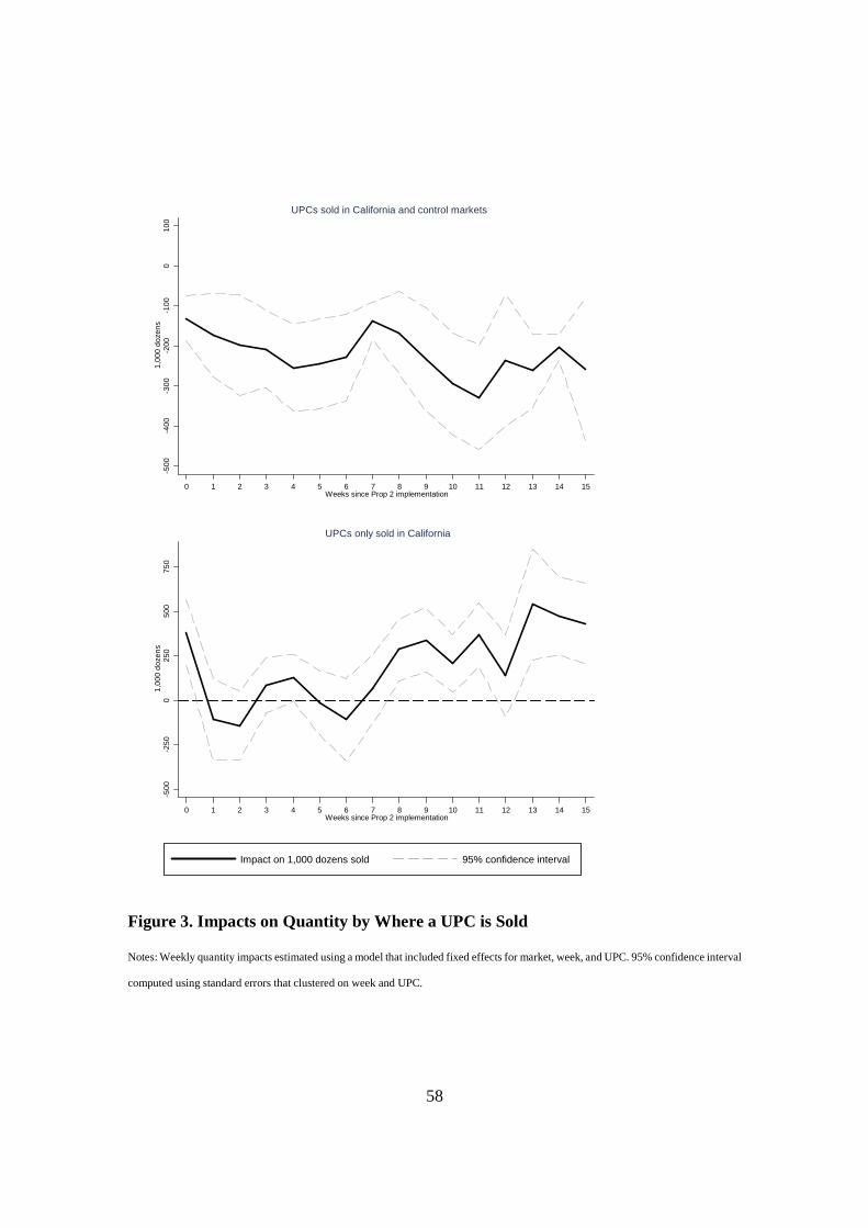
58

Figure 3. Impacts on Quantity by Where a UPC is Sold

Notes: Weekly quantity impacts estimated using a model that included fixed effects for market, week, and UPC. 95% confidence interval

computed using standard errors that clustered on week and UPC.

-500

-400

-300

-200

-100

010

01,

000

doze

ns

0 1 2 3 4 5 6 7 8 9 10 11 12 13 14 15Weeks since Prop 2 implementation

UPCs sold in California and control markets

-500

-250

025

050

075

01,

000

doze

ns

0 1 2 3 4 5 6 7 8 9 10 11 12 13 14 15Weeks since Prop 2 implementation

UPCs only sold in California

Impact on 1,000 dozens sold 95% confidence interval

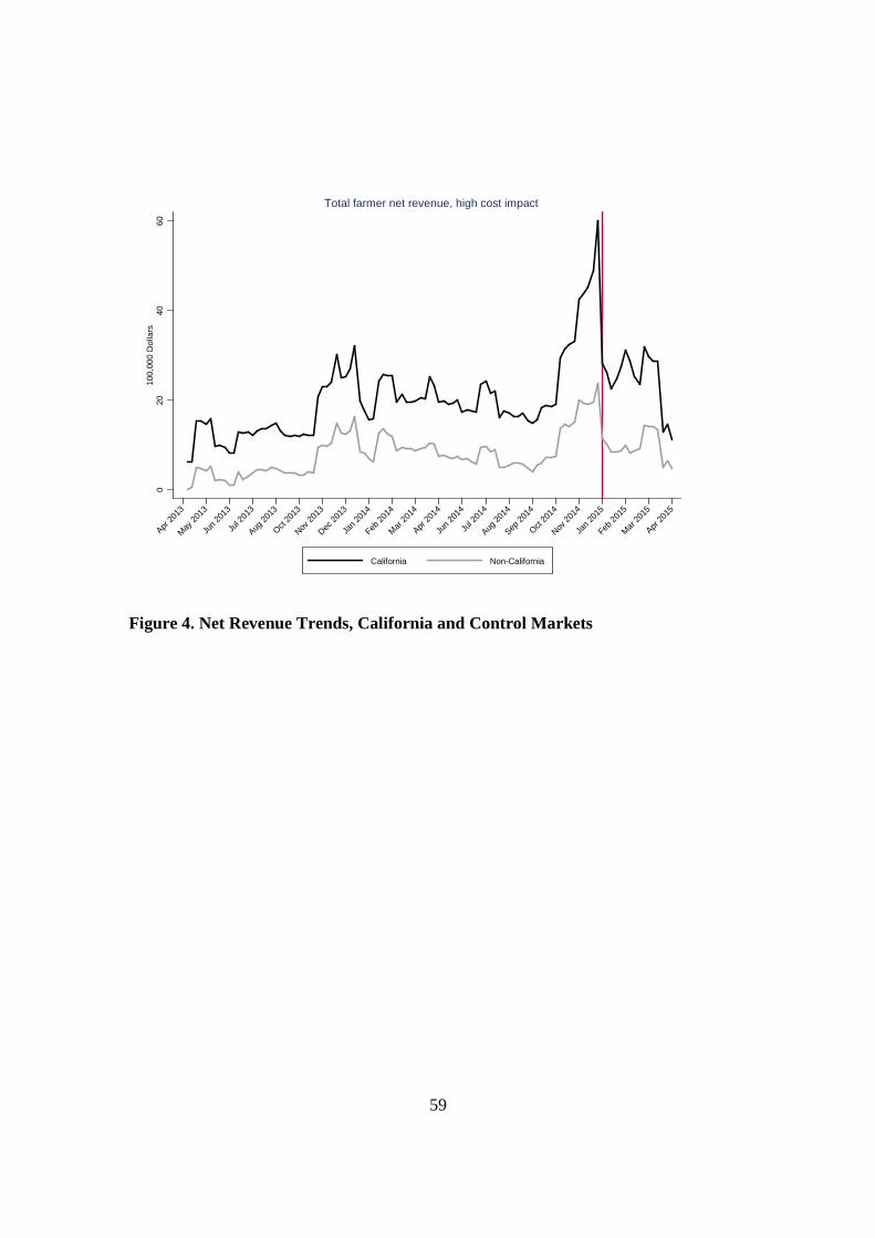
59

Figure 4. Net Revenue Trends, California and Control Markets

020

4060

100,

000

Dol

lars

Apr 20

13

May

201

3

Jun

2013

Jul 2

013

Aug 2

013

Oct 20

13

Nov 2

013

Dec 2

013

Jan

2014

Feb 2

014

Mar

201

4

Apr 20

14

Jun

2014

Jul 2

014

Aug 2

014

Sep 2

014

Oct 20

14

Nov 2

014

Jan

2015

Feb 2

015

Mar

201

5

Apr 20

15

California Non-California

Total farmer net revenue, high cost impact

60

Figure 5. Relationship between Timing of Change in Production Costs and the Impact

of the AW Laws on Net Revenue

Notes: Net revenue impact estimated using a model that included fixed effects for market, week, and UPC. 95% confidence interval

computed using standard errors that cluster on week and UPC.

02

46

8M

illio

ns o

f dol

lars

1 2 3 4 5 6 7 8 9 10 11 12 13 14 15 16 17 18 19 20Beginning of higher costs (weeks prior to Prop 2 implementation)

Impact on net revenue, post Prop 2 95% confidence interval