connecting near and farfield earthquake triggering to...
TRANSCRIPT

1
Connecting near and farfield earthquake triggering to dynamic strain 1
Nicholas J. van der Elst 2
Emily E. Brodsky 3
Department of Earth and Planetary Science, University of California, Santa Cruz 4
5
Abstract: Any earthquake can trigger more earthquakes. This triggering occurs in both 6
the classical aftershock zone, as well as in the farfield. These near and distant 7
populations of triggered earthquakes may or may not be distinct in terms of triggering 8
mechanism. Here we look for a distinction between the two populations by examining 9
how the observed intensity of triggering scales with the amplitude of the triggering strain 10
in each. To do so, we apply a new statistical metric based on earthquake interevent times 11
to a large dataset and measure earthquake triggering as a function of dynamic strain 12
amplitude, where strain is estimated from empirical ground motion regressions. This 13
method allows us to identify triggering at strain amplitudes down to 3×10⁻⁹, which is 14
orders of magnitude smaller than previously reported. This threshold appears to be an 15
observational limit, and suggests that extremely small strains can trigger faults that are 16
sufficiently near failure. We also discover that faults respond in the same way to 17
dynamic strains in both the near and farfield. Surprisingly, there is no need for an 18
additional triggering component to explain the nearfield seismicity rates. Statistical 19
seismicity simulations validate the interevent time method, and strongly suggest that the 20
observed number of triggered earthquakes scales linearly with peak dynamic strain. The 21
empirical connection between dynamic strain and earthquake triggering constitutes a 22
short-term earthquake-forecasting model based on observed seismic shaking. 23

2
24
1. Introduction 25
Triggered earthquakes provide a window into the physics of earthquake nucleation 26
because the forces initiating rupture can be inferred. Because the strain at which a fault is 27
triggered is a measure of its strength, it may be possible to gain insight into the 28
distribution of fault strength by studying the statistics of earthquake triggering [Brodsky 29
and Prejean, 2005; Gomberg, 2001]. In this paper, we use changes in earthquake 30
recurrence times to place a new bound on the minimum strain at which a fault can be 31
triggered and determine how the likelihood of triggering scales with the amplitude of the 32
trigger. 33
34
Estimating the amplitude of the trigger is complicated by the existence of two principal 35
candidate mechanisms for triggering, neither of which is perfectly understood [Freed, 36
2005; Hill and Prejean, 2007]. Static triggering is related to the permanent increase or 37
decrease of stress on one fault due to the coseismic relaxation of stress on another [King 38
et al., 1994]. Dynamic triggering is associated with transient strains carried by radiated 39
seismic waves [Hill and Prejean, 2007]. Static strain changes are permanent, but decay 40
in amplitude quickly with distance away from a fault and are thus unlikely to trigger 41
distant earthquakes. Dynamic strains are generally larger, especially at distance, but 42
present a challenge in explaining prolonged triggering [Brodsky, 2006; Gomberg, 2001]. 43
44
The relative contributions of the two triggering mechanisms are expected to differ as a 45
function of distance from the generative earthquake. Remotely triggered earthquakes are 46

3
believed to result entirely from dynamic triggering, both because static strains are 47
negligible at large distances, and because distant triggering often coincides with the 48
arrival of surface waves [Anderson et al., 1994; Brodsky et al., 2000; Gomberg and 49
Johnson, 2005; Hill et al., 1993; Velasco et al., 2008]. On the other hand, short-range 50
triggering has been attributed to either static or dynamic mechanisms by different 51
researchers [Felzer and Brodsky, 2006; Pollitz and Johnston, 2006; Stein et al., 1994]. 52
Static strains must play a role in determining the location and average rates of 53
earthquakes over long times, because faults are ultimately loaded by quasi-static tectonic 54
motion. Nevertheless, dynamic triggering clearly influences the timing and rate of 55
nearfield earthquakes, as demonstrated by highly directional ruptures, which have 56
asymmetric aftershock zones reflective of the asymmetry in radiation pattern [Gomberg 57
et al., 2003; Kilb et al., 2000]. The relative contribution of the two mechanisms in 58
nearfield triggering remains poorly constrained. 59
60
In this study, we exploit the understanding that dynamic strain dominates farfield 61
earthquake triggering in order to constrain the contribution of static triggering in the 62
nearfield. We first determine an empirical relationship between triggering intensity and 63
dynamic strain in the farfield. Then we compare this farfield relationship to nearfield 64
observations and look for an additional component that would indicate a superposition of 65
static strain triggering on top of the dynamic strain relationship. We ultimately find that 66
earthquake triggering scales with dynamic strain, and that this scaling is identical whether 67
we are looking at remotely triggered earthquakes at distances of hundreds of kilometers, 68
or at local aftershocks triggered within a few kilometers of their mainshock. In the 69

4
process, we develop a measure of earthquake triggering that is significantly more 70
sensitive to low triggering rates than previous measures. 71
72
The first several sections of this article concern the development of the triggering metric. 73
First, we define the interevent time statistic and set up the method for transforming 74
interevent time ratios into an estimate of average triggering intensity within a population 75
of earthquakes. Next, we construct populations on the basis of local dynamic strain and 76
describe the data selection and processing. We then apply the method and show that 77
triggering intensity scales with peak dynamic strain, following the same functional 78
relationship in both the near and farfield triggered earthquake populations. We also 79
report a new maximum bound on the triggering threshold in California of 3×10⁻⁹ strain, 80
several orders of magnitude lower than previous estimates. A statistical seismicity 81
simulation is then used to help interpret and calibrate the results. The simulation strongly 82
suggests that the total number of triggered earthquakes in the real catalog is directly 83
proportional to peak dynamic strain. Finally, we evaluate the implications and robustness 84
of the results. 85
86
2. Measuring earthquake rate changes using interevent times 87
A comparison of triggering rates in the near and farfield requires a metric that can be 88
applied to both populations of earthquakes. This metric needs to be sensitive enough to 89
detect the very small triggering rates associated with the very small strains common to 90
the farfield. Previously, triggered earthquakes have been identified by inspecting 91
seismicity rates [Harrington and Brodsky, 2006; Hill et al., 1993; Stark and Davis, 1996] 92

5
or by filtering waveforms to emphasize short-period energy within the surface wave 93
trains of large, distant earthquakes [Brodsky et al., 2000; Hill and Prejean, 2007; Velasco 94
et al., 2008]. Quantitative estimates of triggering usually involve calculating the 95
likelihood of observing a number of post-trigger events given the previous seismicity rate 96
[Anderson et al., 1994; Gomberg et al., 2001; Hough, 2005]. If the likelihood of the rate 97
increase occurring by chance is low enough, triggering is inferred. 98
99
Any estimate that computes likelihood of triggering based on counting the number of 100
triggered earthquakes relative to a pre-trigger count, like the β-statistic [Matthews and 101
Reasenberg, 1988], is limited in several ways. First, the pre-trigger seismicity rate must 102
be resolved for comparison, and this is inherently difficult. Because most earthquakes 103
occur as clusters of aftershocks, the seismicity rate is always changing. Background 104
seismicity level should therefore be measured at a time as close to the purported trigger 105
as possible in as short a window as possible. Different areas will permit different length 106
windows depending on their background level of seismicity and thus a constant window 107
for an entire dataset may not sufficiently capture the data. Second, an earthquake count 108
can only resolve an integer increase in the number of earthquakes for any individual 109
sequence. A slight advancement in the timing of subsequent earthquakes will only rarely 110
result in a triggered earthquake within the counting time window so only large levels of 111
triggering can be resolved with statistical robustness. Finally, an earthquake count also 112
includes all secondarily triggered earthquakes, that is, aftershocks of aftershocks. These 113
secondary earthquakes are not strictly problematic, because they should still be produced 114
in proportion to the number of primary triggered earthquakes when averaged over many 115

6
events, but they complicate the relationship between trigger amplitude and number of 116
triggered quakes by introducing variance into the measurements. 117
118
To detect triggering at very low dynamic strain amplitudes, our metric must use an 119
adaptive time window to measure background rates, be sensitive to small increases in 120
seismicity rates, and be insensitive to secondary aftershocks. 121
122
2.1 The R-statistic 123
We meet the above requirements by developing a statistic based only on the interevent 124
times between the last earthquake before the trigger and the first earthquake after. The 125
normalized interevent time R is defined by 126
R ≡t2
t1 + t2, (1)
where t1 and t2 are the waiting times to the first earthquake before and after the putative 127
trigger (Figure 1). The R-statistic was originally developed to study triggered quiescence 128
[Felzer and Brodsky, 2005]; we use it here to look for a triggered rate increase. 129
130
The statistic R is a random variable distributed between 0 and 1. The strategy here is to 131
measure the distribution of R on a population of earthquakes that are subject to similar 132
triggering conditions. For instance, the population can be a drawn from a variety of areas 133
subject to the same strain. If there is no triggering and t2 is on average equal to t1, then R 134
is distributed uniformly with a mean value R = 12 . On the other hand, if triggering does 135
occur, t2 will be on average smaller than t1 and R < 12 . More triggering results in a 136

7
smaller R (Figure 2). Therefore, R provides a measure of triggering intensity within a 137
population of earthquakes. 138
139
The R statistic naturally solves the three problems identified with earthquake counting 140
methods by defining an appropriate time window for each event based on the interevent 141
times, utilizing the statistics of large populations, and focusing on the first recorded 142
earthquake rather than the entire triggered sequence. 143
144
One of the unusual features of the R-statistic is that there is no time limit for the inclusion 145
of triggered events. Both immediate and delayed triggering are included in the 146
measurements. This comprehensiveness is desirable because of issues of catalog 147
completeness, as well as the physical implications of delayed triggering. We will return 148
to the issue of delayed triggering at the end of the paper after the statistic has been 149
implemented. 150
151
2.2. Interpreting R as seismicity rate change 152
The mean of R qualitatively captures the intensity of triggering, but as of yet we have no 153
theoretical basis for interpreting R in terms of seismicity rate changes. Interpreting 154
interevent times in terms of the number of expected earthquakes requires the introduction 155
of a probabilistic model for earthquake recurrence. This is equivalent to the common use 156
of probabilistic models to get expected interevent times from earthquake counts 157
[Reasenberg and Jones, 1989]. 158
159
8
If earthquake recurrence were perfectly periodic and uniform, Equation 1 could be simply 160
rearranged to solve for the fractional increase in earthquake rate as a function of the 161
measured R . A somewhat more sophisticated model for earthquake recurrence is a step-162
wise homogeneous Poisson process, in which earthquakes occur randomly in time with 163
an average rate λ1 before the trigger and a new average rate λ2 afterward. We could also 164
use an inhomogeneous Poisson process, where the triggered earthquake rate decays with 165
time according to Omori’s law [Reasenberg and Jones, 1989]. 166
167
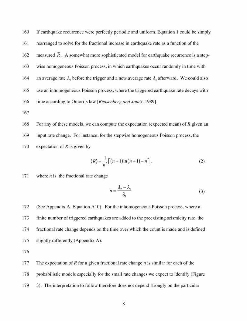
For any of these models, we can compute the expectation (expected mean) of R given an 168
input rate change. For instance, for the stepwise homogeneous Poisson process, the 169
expectation of R is given by 170
R =1n2
n +1( ) ln n +1( ) − n⎡⎣ ⎤⎦ , (2)
where n is the fractional rate change 171
n =λ2 − λ1λ1
(3)
(See Appendix A, Equation A10). For the inhomogeneous Poisson process, where a 172
finite number of triggered earthquakes are added to the preexisting seismicity rate, the 173
fractional rate change depends on the time over which the count is made and is defined 174
slightly differently (Appendix A). 175
176
The expectation of R for a given fractional rate change n is similar for each of the 177
probabilistic models especially for the small rate changes we expect to identify (Figure 178
3). The interpretation to follow therefore does not depend strongly on the particular 179

9
probability model used. This is because we are looking only at the time to the first event, 180
and not the distribution of times to subsequent events, where most of the differences exist 181
between the models. 182
183
For the rest of this paper, we use the step-wise homogeneous Poisson model, because it is 184
the simplest stochastic model, has an analytical solution, and does not require 185
independent calibration of the background seismicity rate. By the method of moments 186
[Casella and Berger, 2002], we set the expectation of R equal to the measured sample 187
mean, R , and solve numerically for n. Because the transformation from R to n is 188
somewhat model dependent, the calculated fractional rate change n is hereafter referred 189
to as triggering intensity and interpreted as a qualitative measure of rate change that 190
illuminates the scaling of triggering intensity within populations. We will ultimately use 191
statistical simulations to calibrate n and get a quantitative estimate of number of 192
earthquakes triggered for a given strain. 193
194
3. Defining Populations 195
The R-statistic measures triggering intensity in a population of earthquakes. Therefore, 196
the first step in applying R to a real dataset is to define reasonable populations so that we 197
can evaluate the different rate changes in each one. 198
199
Because long-range triggering is clearly associated with dynamic strain, we start by 200
constructing sets of earthquakes with a common dynamic strain. Dynamic strain is 201
proportional to the amplitude of seismic waves 202

10
ε ~ AΛ~ VCS
, (4)
where A is displacement amplitude, Λ is wavelength, V is particle velocity and CS is 203
seismic wave (phase) velocity [Love, 1927]. In principle, dynamic strain can therefore be 204
calculated wherever there is a seismogram. Ground motions are converted to strain by 205
dividing by wavelength or wave speed, depending on whether the regression is for 206
displacement or velocity, respectively. In the nearfield, S-waves are the largest motion, 207
and in the farfield, surface waves are larger. Both have a phase velocity CS of ~3.5 km/s. 208
209
Previous work has investigated the accuracy of using ground motions as a proxy for 210
strain at depth by comparing strain estimated from seismometer data to strain measured 211
by strainmeters [Gomberg and Agnew, 1996]. This work found that seismometer data 212
predicted strain amplitudes within ±20% of the strainmeter measurements. 213
214
3.1. Estimating strain with empirical ground motion regressions 215
In order to take full advantage of the large number of earthquakes in the catalog, we must 216
calculate strain at any point on the map for any trigger in the catalog, not only where we 217
have seismic stations and archived waveforms. Fortunately, peak empirical ground 218
motions are well studied in the nearfield for engineering purposes and at regional and 219
teleseismic distances for calibrating magnitude scales [Boatwright et al., 2003; Joyner 220
and Boore, 1981; Lay and Wallace, 1995; Richter, 1935]. We use these regressions to 221
estimate ground motion as a function of distance and magnitude for nearfield and farfield 222
waves, respectively. 223

11
224
Specifically, for long-range strain we use the surface wave magnitude relation [Lay and 225
Wallace, 1995], 226
log10 A20 = MS −1.66 log10 Δ − 2 , (5)
where A20 is in µm and Δ is in degrees. This equation is commonly used to assign a 227
catalog magnitude based on a measured amplitude at some distance. We turn the 228
procedure around and use the catalog magnitude to calculate an amplitude. This 229
approach uses the long-period waves (T=20 s) as indicators of the peak strain, implicitly 230
assuming that the short-period body waves are attenuated at large distances. The 231
displacement A is converted to velocity for the 20 second waves as V = 2πA20 T [Aki 232
and Richards, 2002]. Equation 5 was historically calibrated using a similar catalog of 233
global earthquakes to the one we use for potential triggers, and so provides a good 234
measure of average amplitude despite being imperfect for any individual earthquake. 235
The equation is designed for distances on the order of at least 800 km [Lay and Wallace, 236
1995]. This sets the minimum distance for the population of long-range triggers. 237
238
The amplitude of the short-range triggers is calculated from an empirical peak ground 239
velocity regression determined from California ShakeMap data, 240
log10V = 1.06ML − 0.0063r − log10 r +1.35 , (6)
where V is velocity in µm/s, r is distance in km, and ML is Richter magnitude [Boatwright 241
et al., 2003]. The reported uncertainties in the constants are: 1.06±0.02, 0.0063±0.002 242
and 1.35±0.23, corresponding to a variation of about one half order of magnitude in the 243
observed wave amplitude associated with any individual earthquake. Considering the 244
12
additional uncertainty associated with estimating strain from seismometer data, we 245
consider our estimates accurate within an order of magnitude. 246
247
3.2. Constructing Populations Over Space 248
The interevent time method only looks at single earthquake pairs bracketing a potential 249
trigger, but a large quake may trigger numerous earthquakes throughout the study area. 250
We therefore split the study region into spatial bins and calculate R for each of these bins 251
(Figure 4). This allows us to get a robust distribution of R-values for each trigger and 252
ensures that the measurements are not dominated by whichever aftershock sequence is 253
most active at the time. Using a spatial bin that is much smaller than the wavelength of 254
the long-range trigger also ensures that measured triggering intensity reflects the strain at 255
that site. 256
257
The higher the number of bins, the higher the number of bracketing pairs for each trigger 258
quake, down to a lower size limit where single earthquakes begin to be isolated. A bin 259
size of 0.1º×0.1º gives the maximum number of bracketing pairs for the whole catalog of 260
potential triggers, but we perform the analysis using several different bin sizes to ensure 261
robustness of the results with respect to parameter choices. 262
263
To measure nearfield triggering, we use a disk centered on the mainshock epicenter. The 264
radius of the disk is set to give the same area as the long-range bins. Because the R 265
statistic is calculated over an area around the mainshock epicenter, a mean peak velocity 266
is calculated over that area. Assuming radial symmetry and neglecting the inelastic 267

13
attenuation term (2nd term on right hand side of Equation 6) at these small distances, the 268
average peak velocity is 269
V D( ) = 1πD2 V r( )2πr dr ≈ 2 ⋅101.06ML +1.35
0
D
∫ ⋅D−1 , (7)
where V(r) was defined in Equation 6 and D is the radius of aftershock collection. 270
271
3.3 Earthquake Catalogs 272
Using the R statistic on earthquake populations requires large accurate catalogs for both 273
potential trigger earthquakes and for local seismicity. The trigger catalog is drawn from 274
the global ANSS catalog from 1984 through April 2008. A depth cutoff is imposed at 275
100 km, because deep earthquakes do not generate significant surface waves. Only 276
earthquakes with surface wave amplitude greater than ten micrometers displacement are 277
treated as potential triggers, because preliminary work finds no observable triggering 278
signal at this or lower amplitudes. This minimum corresponds to a MS4.5 earthquake at 279
800 km. We show below that this cutoff is below the observational threshold for long-280
range triggering. 281
282
Both potential long-range triggered quakes and potential nearfield triggers are drawn 283
from the ANSS catalog for the California study region. Other catalogs have considerably 284
smaller location errors than the ANSS catalog, but contain considerably fewer 285
earthquakes. Location error should not be a significant source of error for this study, 286
because the required spatial precision is on the order of the spatial bin size. We therefore 287
choose the catalog with the largest number of earthquakes. The interevent time method 288
should not be sensitive to regional variations in completeness magnitude, because the 289

14
incompleteness should affect the pre and post-trigger catalogs in a consistent way. 290
However, we impose a magnitude threshold of 2.1, based on the roll-off in the Gutenberg 291
Richter distribution for the catalog as a whole, to protect against large swings in 292
completeness level with time. The study area extends from 114° to 124° west, and from 293
32° to 42° north. 294
295
We also look at the scaling of triggering intensity with dynamic strain in Japan. Here we 296
use the JMA catalog from 1997 through March 2006. For consistency with California, 297
we limit the catalog of local events to shallower than 15 km within the land area of the 298
four main islands of Japan. The magnitude of completeness for the JMA catalog of 299
shallow crustal events is below 2.1, but we impose this larger magnitude cutoff for 300
consistent comparison with California. 301
302
3.4. Practicalities of Implementation 303
In order to evaluate the significance of R as an indicator of triggering, we require 304
confidence bounds on R . We use the bootstrap method to generate confidence bounds by 305
randomly resampling the R distribution for a given population to generate a suite of 306
estimates of R [Casella and Berger, 2002]. 307
308
We also take into consideration two potential sources of undesirable bias for realistic sets 309
of earthquakes. One is related to the superposition of Omori’s law on measurements 310
made in aftershock sequences, and the other to the finiteness of the earthquake catalog. 311
312

15
For the farfield case, the timing of the distant trigger is usually uncorrelated to the timing 313
of earlier (or non-triggered) quakes in the study region, because of the large spatial 314
separation. However, this is not the case for short-range triggered earthquakes, where an 315
Omori-type rate decay (~t-1) may be superimposed on the timing of both the trigger quake 316
and the subsequent triggered quake. This decay biases the R statistic toward higher 317
values and obscures the triggering signal. We suppress this bias by requiring that the 318
trigger event be much larger than the immediately preceding event, ensuring that the 319
average rate increase due to the trigger will be much larger than the Omori-law rate 320
decrease superimposed on the entire sequence. A higher magnitude difference better 321
insures against bias, but significantly reduces the number of eligible trigger quakes. We 322
find that R is stable for a minimum magnitude difference of one unit. One magnitude 323
unit corresponds to a roughly tenfold increase in total triggering power, and Omori’s law 324
ensures that the difference is in general much greater than this, because the influence of 325
the previous earthquake decays rapidly with time. 326
327
Another potential source of bias is related to the finiteness of the catalog. This is 328
especially problematic in regions where seismicity rates are low. To understand this 329
effect, consider a putative trigger near the beginning of the catalog. The probability that 330
the first prior event occurs before the start of the catalog is much greater than the 331
probability that the first subsequent event occurs beyond the end, simply because of the 332
position of the trigger quake within the catalog. Since we cannot measure t1 for 333
earthquakes that occurred before the start of the catalog, we only calculate R when t1 is 334
unusually small, and therefore obtain disproportionately large values of R. The mean R 335

16
can thus be biased by the non-uniform distribution of global trigger times. We determine 336
the bias numerically by measuring R in 1000 simulations using the real trigger times, but 337
with local catalogs consisting of uniformly distributed random times. This calculated 338
bias is subtracted from the values of R measured for the actual catalog. For simplicity, 339
the bias-corrected mean is referred to below as R . 340
341
4. Observed Triggering Intensity as a Function of Dynamic Strain 342
We begin attacking real data by measuring the interevent times for a well-known case of 343
pervasive triggering in order to establish that R and n behave as designed. The 2002 344
magnitude 7.9 Denali earthquake generated peak dynamic strains on the order of 2-3×10⁻⁷ 345
for the California study area, according to the empirical regressions, and is known to have 346
triggered significant seismicity [Anderson et al., 1994; Gomberg et al., 2004]. For this 347
initial case study, we disregard amplitude variations and define a population consisting of 348
the full study area. The resulting R distribution reflects significant triggering (Figure 5). 349
The sample mean R (with 95% confidence limits) is 0.475 (0.461-0.488), corresponding 350
to a fractional rate change of 0.16 (0.08-0.26) according to Equation 2. A simple 351
earthquake count before and after the Denali earthquake indicates a 22% seismicity rate 352
increase in the following 24 hours. These estimates agree within error. We conclude that 353
R is capable of capturing triggering in a case with known seismicity rate increases. 354
355
The real utility of the method becomes apparent when it is applied to the full ANSS 356
dataset with over 3000 potential farfield triggers, and 12,000 nearfield triggers meeting 357
our criteria. Figure 6 shows measured R distributions for different dynamic strain 358

17
amplitudes, corresponding to various combinations of magnitude and distance for the 359
long-range dataset, and various magnitudes at constant distance for the short-range data. 360
The R-distributions show evidence of both immediate triggering, in the form of large 361
spikes near R=0, and protracted triggering, in the form of a continuing decrease with 362
increasing R. The distributions show larger proportions of small R for higher strain 363
levels, as expected. 364
365
Triggering intensity for the entire dataset, computed according to Equation 2, is plotted in 366
Figure 7. Triggering intensity scales continuously with peak dynamic strain over five 367
orders of magnitude in strain amplitude. Triggering intensity has the same relationship to 368
peak dynamic strain in both long and short-range populations. There is no increase in 369
triggering intensity in the nearfield that requires an additional triggering component. The 370
continuity shows that long-range triggered earthquakes are no more rare or unusual than 371
expected given the amplitude of dynamic strains at distant sites. For very small farfield 372
strain levels, the triggering is rare and difficult to identify, but does not differ in a 373
fundamental way from triggering at higher strain levels in the nearfield. 374
375
The apparent triggering threshold in California is 3x10⁻⁹ strain, where the threshold is 376
defined as the strain at which triggering intensity n is non-zero (or equivalently R < 0.5 ) 377
at the 95% confidence level. This threshold is not dependent on the transformation from 378
R to triggering intensity n. For a crustal shear modulus of 30 GPa, this corresponds to a 379
stress of 0.1 kPa. This estimate is several orders of magnitude smaller than previously 380
reported for dynamic triggering [Brodsky and Prejean, 2005; Gomberg and Davis, 1996; 381

18
Gomberg and Johnson, 2005; Stark and Davis, 1996]. Previous estimates have been 382
based on counting statistics. If n>1, the change in seismicity rate is comparable to the 383
background rate, and triggering is easily observable by counting methods. For a Poisson 384
process, the variance is equal to the average rate, so n>1 also roughly corresponds to the 385
threshold for statistical significance using an earthquake count. Therefore, only the 386
seismicity rate increases corresponding to n>1, i.e. strains of nearly 10-5, were easily 387
observable in previous studies. 388
389
The strain threshold is smaller than tidal stresses [Cochran et al., 2004; Scholz, 2003]. 390
This is somewhat puzzling, because tidal stresses might be expected to “clean out” all 391
available nucleation sites on a daily basis and set a lower limit for dynamic triggering. 392
Strain tensors associated with crustal earthquakes are likely oriented with more variety 393
than those due to the tides, however, and may access faults that tidal strains are incapable 394
of triggering. In addition, the forcing at the relatively long periods of the tides may be 395
intrinsically different from the dynamic strains imposed at the short periods of seismic 396
waves [Beeler and Lockner, 2003; Gomberg et al., 1997; Savage and Marone, 2008] 397
398
Triggering intensity in shallow crustal Japan (Figure 7b) is reduced relative to California 399
in both the long and short-range populations, with a higher triggering threshold of 10-6 400
strain. However, where long-range strain is large enough to overlap in amplitude with 401
short-range strain, the triggering intensity in the long and short-range earthquake 402
populations is identical. This overlap further reinforces the continuity observed in Figure 403
7a. The relative absence of long-range triggering in Japan has been documented before 404

19
[Harrington and Brodsky, 2006], but this study shows that the reduced triggering 405
susceptibility extends to the nearfield, as well. This difference in triggerability may 406
reflect the difference in tectonic style (compressive vs. transpressive) between the two 407
study areas. 408
409
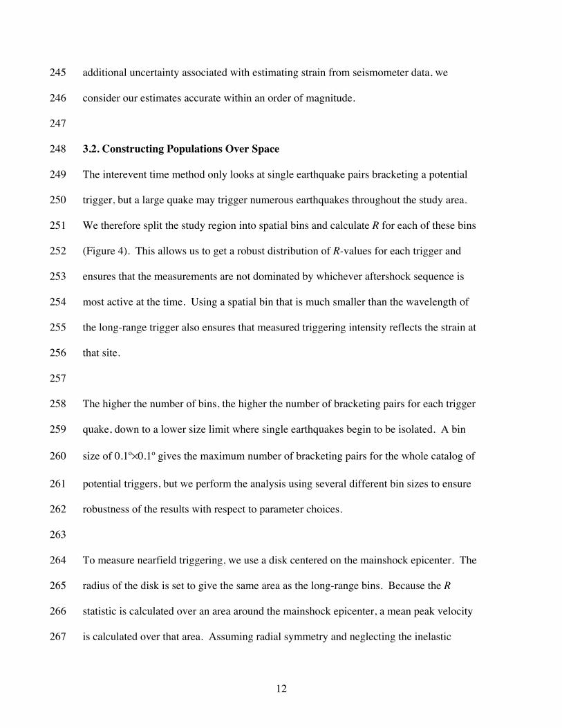
Evaluating the probability of triggering as a function of strain (Figure 8) provides an 410
interpretation of the observed triggering threshold. Probability is calculated from the 411
triggering intensity n using the same Poissonian statistical model as before (Appendix B). 412
The probability of triggering an earthquake within its own recurrence interval, as a 413
function of n, is given by 414
P NEQs ≥ 1( ) = 1− exp − n +1( ){ } . (8)
The baseline probability of having an earthquake in the absence of any rate change (n=0) 415
is 63%. A positive n produces a positive probability gain. Figure 8 shows that the 416
probability gain decreases smoothly to zero as n decreases. For the ~10-9 strain bin in 417
California, there are ~105 interevent time measurements (~103 triggers x ~102 local 418
earthquakes) and this number of events is sufficient to establish the statistical significance 419
of the 0.003% probability gain observed. An order of magnitude more observations 420
would be needed to push the observable threshold an order of magnitude lower. This 421
exceeds the size of the earthquake catalog, and we infer that the absence of detected 422
triggering at strains of less than 10-9 reflects an observational limit and not a physical 423
threshold. 424
425
5. Validation and calibration through statistical seismicity simulations 426

20
We have shown that there is a continuous trend in the scaling of triggering intensity with 427
dynamic strain in both near and farfield populations. However, there is a problem 428
interpreting the slope of this trend. Previous work using earthquake counting and 429
carefully declustered seismicity catalogs has shown that the number of local aftershocks 430
following a mainshock of magnitude M goes as 10αM , with α=1 [Felzer et al., 2004; 431
Helmstetter et al., 2005]. This study finds that triggering intensity n varies as 100.5M 432
(Figure 7). We will now show that this discrepancy arises from the application of a 433
probability model derived for isolated earthquake sequences to a catalog containing 434
superimposed triggering cascades. Fortunately, this effect can be quantified and 435
calibrated using statistical simulations. 436
437
As described in Section 2.3, triggering intensity is estimated from inter-event times using 438
a probabilistic model for earthquake recurrence times. None of the models described 439
consider the effect of the earthquake cascade on the estimation of rate change. The 440
transformation from R to n implicitly assumes that we correctly associate earthquakes 441
with their respective triggers, but a real catalog contains numerous superimposed 442
triggering cascades. The first earthquake before and after a prospective trigger may or 443
may not then be causally related. If they belong to a different earthquake sequence, they 444
will introduce R-values sampled from a uniform distribution, and the resulting 445
distribution will be some combination of the two curves illustrated in Figure 2. This has 446
the effect of dampening the observed triggering signal. 447
448
To evaluate whether the presence of superimposed earthquake cascades can explain the 449

21
discrepancy between our recovered slope in Figure 7 and previous work based directly on 450
earthquake counts, we generate an artificial earthquake catalog that follows the usually 451
observed statistics of magnitude, timing, and triggering distributions (Appendix C). A 452
well-established method for generating such a catalog is the epidemic triggered 453
aftershock sequence (ETAS) [Ogata, 1992]. ETAS uses well-known empirical statistical 454
seismicity laws as probability distributions to generate stochastic seismicity catalogs 455
(Appendix C). Numerous researchers have used ETAS models to study the complex 456
statistical repercussions of simple earthquake cascades [Felzer et al., 2002; Felzer et al., 457
2004; Hardebeck et al., 2008; Helmstetter and Sornette, 2003; Holliday et al., 2008]. 458
Here we use ETAS to study the effects of superimposed earthquake triggering sequences 459
on our measure of triggering intensity. 460
461
We first apply the R statistic to a zero-dimensional ETAS catalog. The zero dimensional 462
model simulates earthquakes in time only, disregarding spatial distribution, in order to 463
isolate the effect of the earthquake cascade. The triggering law in the simulation 464
corresponds to the case of the inhomogeneous Poisson process with an Omori decay 465
(Appendix A), and the number of triggered earthquakes scales with α=1. The 466
inhomogeneous Poisson model for interevent times is used to transform R to a triggered 467
rate change. 468
469
Because causality is known in the simulation, we can investigate how the use of the first 470
earthquake before and after the trigger affects the recovered scaling relationship. If 471
interevent times are measured with respect to known branches of the cascade, that is, if 472

22
the causal relationships are known, the transformation from R recovers the scaling law 473
that was put into the model (Figure 9a). If we instead use the first earthquake before and 474
after a putative trigger, a scaling with α=0.5 is recovered, similar to that recovered for the 475
real catalog (Figure 9b). This demonstrates that the discrepancy between our scaling and 476
that found in other studies is due to the inclusion of some non-causally related interevent 477
times in the R distribution. Our interevent time observations are, in fact, consistent with 478
the number of triggered earthquakes being directly proportional to strain, as found in 479
previous studies. Consequently, the triggering intensity calculated by our transformation 480
represents a lower bound on the real fractional rate change. 481
482
Triggering intensity n (Equation 2) should be a good measure of earthquake rate as long 483
as it scales in a consistent manner with R . The zero-dimensional simulation shows that 484
n indeed scales consistently, but this simulation only considered nearfield aftershock 485
triggering, not triggering from distant earthquakes unconnected to the local earthquake 486
cascade. It is not immediately obvious that the effect of unknown parentage will be 487
identical in the near and farfield. Since we interpret the continuity in the scaling from 488
farfield to nearfield as indicative of continuity in the triggering physics, we need to verify 489
that the continuity is robust despite the imperfect transformation. 490
491
To verify the robustness of the continuity of the near and farfield trends, we now apply 492
the R statistic to a full space-time simulated ETAS catalog. ETAS models have generally 493
been used to study near and intermediate-field triggering. We make a key modification 494
to the model in order to introduce far field triggering, replacing the aftershock 495

23
productivity law and the spatial clustering kernel with the simple rule that earthquakes 496
are triggered in direct proportion to dynamic strain. In practice, this means adjusting the 497
parameters of the standard empirical descriptions to match the magnitude and distance 498
components of the empirical ground motion regressions. Suggestively, this requires only 499
a slight modification of the parameters estimated by Felzer [2002] and Hardebeck et al., 500
[2008]. We are then able to generate both normal aftershock triggering and long-range 501
triggering due to distant sources in the same simulated earthquake catalog. The 502
productivity constant for long-range triggers is set to match the proportionality in the 503
nearfield (Appendix C), and comes to about 300 earthquakes km-2 per unit strain. 504
505
Applying the R statistic to the simulated catalog, we recover the continuous trend 506
observed in the real data for several ETAS parameter sets taken from the literature (Table 507
1; Figure 10). The log-slope of the trend (α) is different for different simulation runs, 508
and correlates most strongly with the fraction of triggered earthquakes generated in a 509
particular realization (Figure 10d). We interpret this as meaning that for a higher fraction 510
of triggered events (low background fraction), there is a higher probability that the 511
earthquakes used to compute R are related to some other ongoing sequence rather than 512
the putative trigger, introducing a higher proportion of uniformly distributed samples into 513
the R distribution. As a result, the recovered slope correlates with the proportion of 514
background earthquakes in the final simulated catalog. The precise relationship between 515
the absolute value of n and the other statistics of the catalog is beyond the scope of this 516
study. 517
518

24
Importantly, the continuity between the long and short-range trends is robustly recovered 519
for all simulations. The simulation that best matches the observations (Figure 10a) has a 520
background fraction of ~25%. This is in agreement with the most recent estimates for 521
California seismicity, which put the background fraction at ~18-24% [Hainzl et al., 522
2006; Marsan and Lengline, 2008]. The agreement between the simulation and the 523
observations is remarkable in that the parameters going into the simulation are based on 524
aftershock numbers and rates [Felzer et al., 2002], and are not tuned to match the 525
interevent time observations. The assignment of all aftershock production to dynamic 526
strain is required in order to explain the observed interevent times in the nearfield, given 527
the model assumption that intensity of triggering falls off according to Omori’s law. This 528
suggests that roughly 75% of the earthquakes in the real seismicity catalog are 529
dynamically triggered. The agreement between the observed and simulated data in the 530
farfield is also remarkable, given that the modeled triggering rate is based only on the 531
proportionality observed in the nearfield. 532
533
The ETAS simulation validates the interpretation with respect to the continuity of the 534
trend and strongly suggests that the real data reflect a direct proportionality between 535
fractional rate change and peak dynamic strain, with a productivity of ~300 earthquakes 536
km-2 per unit strain. 537
538
6. Discussion 539
6.1 Implications for dynamic triggering 540
Peak dynamic strain is a good empirical predictor of triggering intensity in both the near 541

25
and farfield (Figure 7). This continuity from the farfield, where we know that all 542
earthquakes are triggered dynamically, into the nearfield, implies that dynamic strains 543
determine the timing and rate of earthquake triggering at all distance. How do dynamic 544
strains, which produce no permanent load change, nonetheless dominate earthquake 545
triggering rates? The low threshold for dynamic triggering suggests that arbitrarily small 546
dynamic strains can trigger earthquakes on nucleation sites that are sufficiently near 547
failure. Without a physical threshold for dynamic triggering, the question becomes one 548
of a balance of timescales -- the timescale over which a nucleation site is loaded to failure 549
quasi-statically vs. the time between dynamic strain events large enough to push the fault 550
the rest of the way. If the dynamic trigger recurrence time is smaller than the quasi-static 551
time to failure, the fault will be triggered dynamically. A fault far from failure is unlikely 552
to be triggered by any but the largest dynamic strain events. However, as the fault nears 553
failure, not only are smaller and smaller dynamic strains required for triggering, but the 554
availability of sufficient triggers increases due to the greater abundance of small 555
earthquakes. 556
557
In fact, a simple scaling argument shows that a fault is just as likely to be triggered by a 558
small strain event as by a large one. We have shown that the number of dynamically 559
triggered earthquakes is linearly proportional to strain. The peak dynamic strain 560
increases as ~10M, so the number of triggered earthquakes for a given strain event also 561
goes as 10M. The Gutenberg-Richter distribution gives that the number of earthquakes 562
with magnitude M goes as ~10-M. Therefore, the total triggering power for each 563
magnitude bin as a whole is constant with respect to the amplitude of the dynamic strain; 564

26
(9)
Small earthquakes with magnitudes below the level of catalog completeness are therefore 565
very important in triggering subsequent earthquakes. The cascade model implies that the 566
duration and total number of earthquakes triggered in any given sequence is therefore 567
strongly dependent on the magnitude of the smallest physically possible earthquake 568
[Sornette and Werner, 2005]. Similar arguments for the importance of small earthquakes 569
have been made previously based on statistical considerations [Felzer et al., 2004; Felzer 570
and Brodsky, 2006; Helmstetter et al., 2005]. 571
572
6.2 How delayed earthquakes can be triggered earthquakes 573
Earthquakes arbitrarily delayed from the mainshock are allowed to contribute to the 574
triggering signal in the measurements made here. We choose not to limit the delay time 575
for triggering for several reasons. First, primary triggered earthquakes may be obscured 576
by the passage of the generative seismic waves. This is especially true for nearfield 577
triggering, where it has been demonstrated that a tremendous number of early aftershocks 578
are usually missing from earthquake catalogs [Kagan, 2004; Peng et al., 2007]. In this 579
case, the first earthquake in the catalog may actually be a secondarily triggered 580
earthquake, that is, an aftershock of an obscured, directly triggered quake [Brodsky, 581
2006]. The timing of the delayed secondary quake provides a lower bound on the rate 582
increase associated with the direct triggering. Furthermore, if the Gutenberg-Richter 583
relationship holds for magnitudes much smaller than the completeness magnitude, many 584
small directly triggered quakes will not make it into the catalog, but may still play an 585
N !( ) = NTriggers "NTriggered
N !( )#10M "10$M= constant

27
important role in prolonging the aftershock sequence, as demonstrated by Equation 9. 586
588
Second, it is possible that dynamic strains trigger earthquakes by inducing a semi-589
permanent change in the properties of the fault patch, rather than only through transiently 590
exceeding the fault strength. Several studies have posited long-lasting changes in the 591
mechanical properties or effective stresses within fault zones related to the passage of 592
high-amplitude seismic waves. [Brodsky et al., 2003; Elkhoury et al., 2006; Johnson and 593
Jia, 2005; Parsons, 2005]. Delayed triggering may then simply reflect the prolonged 594
nature of the triggering process. 595
596
Regardless of whether delayed triggering reflects an incompletely observed earthquake 597
cascade or a prolonged physical perturbation of the fault conditions, uncorrelated (non-598
triggered) events are sampled from a uniform distribution of R values, and their inclusion 599
will mute the triggering signal but not introduce a bias in the mean. 600
601
6.3. Robustness of the observations with regard to parameters 602
The binning of the data and the separation of triggered quakes into farfield and nearfield 603
populations required the introduction of some arbitrary parameters. We want to be 604
certain that the continuity in triggering intensity between the near and farfield populations 605
can be interpreted as a continuity in the triggering mechanism. The success of the 606
statistical simulation in reproducing the observations lends some confidence to this 607
interpretation, but we also check the robustness of the results with respect to the data 608
selection parameters. 609

28
610
The first arbitrary parameter is the spatial bin size. The results shown in Figure 7-8 use a 611
bin size of 0.1º, because this maximizes the number of R values we can calculate. Figure 612
11 confirms that the continuous scaling is not sensitive to the spatial bin size, as long as 613
the number of data points remains high. We show results for bin sizes between ~8 km2 614
and 123 km2 (0.025º - 0.1º on a side). For larger bins, either the reduced quantity of data 615
or the masking of triggered activity by unrelated local aftershocks causes confidence 616
limits to exceed the mean triggering signal for the farfield data. 617
618
The distance cutoff for farfield triggers also does not influence the results. Trials using 619
minimum far-field cutoff distances of 800 km through 3200 km also recover the 620
continuous scaling (Figure 12). The variance in R begins to overwhelm the triggering 621
signal with cutoffs above 3200 km, due to the diminished dataset, and the surface wave 622
magnitude relationship is not valid for distances less than the order of 800 km, as 623
mentioned before. 624
625
Finally, to make sure the long-range triggering signal is not generated entirely by isolated 626
geothermal areas, we plot the contribution of each spatial bin to the total measured 627
triggering intensity, combining all the farfield amplitude bins (Figure 13). Geothermal 628
regions (particularly Long Valley and the Salton Trough) contribute strongly, as 629
expected, but virtually all regions of active seismicity in California contribute to the long-630
range triggering signal. 631
632

29
6.4 Relation to previous work 633
Dividing earthquakes into populations with common strain is a novel way of looking at 634
the scaling of triggering intensity with dynamic strain. Previous work has shown the 635
relevance of dynamic triggering in the nearfield by comparing the falloff in aftershock 636
density away from a mainshock to the falloff of seismic waves at near and intermediate 637
distances [Felzer and Brodsky, 2006; Gomberg and Felzer, 2008]. These correlations 638
cannot be trivially mapped to a particular function of dynamic strain, however, because 639
the decay in triggering intensity is superimposed on the decay of available nucleation 640
sites away from the mainshock. It therefore becomes necessary to carefully analyze the 641
statistics of non-triggered (background) seismicity in order to extract the triggering 642
function. The method defined here does not suffer from this ambiguity, because each 643
value of R that goes into a distribution measures the change in seismicity rate at a single 644
site. Since we use various combinations of magnitude and distance for the farfield case, 645
and various magnitudes but constant distance for the nearfield case, there is not a one-to-646
one relationship between dynamic strain and distance from the mainshock in these 647
populations. We therefore do not need to be concerned about the geometry of the local 648
fault network. 649
650
7. Conclusion 651
The observations presented here have the following implications: (1) extremely small 652
strains can trigger faults if they are sufficiently near failure, down to observed levels of 653
3×10⁻⁹ strain. (2) Dynamic strain events are frequent enough and productive enough to 654
control the timing of the majority of aftershocks, generating roughly 75% of the 655

30
earthquakes in the California seismicity catalog. (3) There is no qualitative distinction 656
between long-range triggered earthquakes and aftershocks. 657
658
These observations place strong constraints on mechanisms of earthquake nucleation. 659
Furthermore, the empirical connection between triggering rate and dynamic strain lays 660
the foundation for a probabilistic description of earthquake clustering based on 661
instrumentally observed seismic wave amplitudes. This has major implications for time-662
dependent forecasting of earthquakes. 663
664
Appendix A: Expectation of R for a Poisson process with a step change in intensity 665
To find the expectation of R, we first derive the distribution of R by transforming the 666
probability density functions for the times to the first events before and after the trigger, 667
t1 and t2. 668
669
The interevent times in a Poisson process follow an exponential distribution with the 670
general form 671
f t( ) = λ t( )exp − λ t( )dt
0
t
∫{ } (A1)
where λ(t) is the intensity, or average rate of earthquakes, at time t. The joint distribution 672
of the two independent recurrence times is then the product of two exponential 673
distributions. Defining 674
N t( ) = λ t( )dt
0
t
∫ (A2)
the joint distribution of the interevent times is 675

31
f (t1,t2 ) = λ1 t1( )λ2 t2( )exp −N1 t1( ) − N2 t2( ){ } . (A3)
where subscripts 1 and 2 refer to the rates before and after the trigger respectively. 676
677
We derive the joint distribution of R, where 678
R =t2
t1 + t2, (A4)
and another arbitrary variable, e.g. T = t2 , by substituting the inverse definitions of R and 679
T into Equation A3 and multiplying by the absolute value of the Jacobian of the 680
transformation [Casella and Berger, 2002]. The Jacobian is given by 681
J = det∂t1
∂R∂t1
∂T∂t2
∂R∂t2
∂T
⎛
⎝
⎜⎜⎜
⎞
⎠
⎟⎟⎟= −
TR2
1R−1
0 1= −
TR2
. (A5)
The joint distribution for R and T is then 682
f R,T( ) = λ1TR− T⎛
⎝⎜⎞⎠⎟λ2 T( )exp −N1
TR− T⎛
⎝⎜⎞⎠⎟− N2 T( )
⎧⎨⎩
⎫⎬⎭TR2
. (A6)
The marginal distribution of R is obtained by integrating Equation A6 with respect to T. 683
The expectation of R is therefore the double integral 684
R = λ1TR− T⎛
⎝⎜⎞⎠⎟λ2 T( )exp −N1
TR− T⎛
⎝⎜⎞⎠⎟− N2 T( )
⎧⎨⎩
⎫⎬⎭TR0
∞
∫01
∫ dTdR . (A7)
685
For the stepwise homogenous Poisson process with a step change in otherwise constant 686
intensity λi, the solution to Equation A7 is 687

32
R =λ1λ2
λ2 − λ1( )2λ1λ2
+ ln λ2λ1
⎛⎝⎜
⎞⎠⎟−1
⎛
⎝⎜⎞
⎠⎟. (A8)
Equation A8 can be expressed as a function of the fractional rate change, 688
n ≡N2 t( ) − N1 t( )
N1 t( )=λ2 − λ1λ1
, (A9)
Note that the second equality in Equation A9 only holds for the cases where λ1 and λ2 are 689
independent of time. 690
691
Substituting Equation A9 into Equation A8 yields, 692
R =1n2
n +1( ) ln n +1( ) − n⎡⎣ ⎤⎦ . (A10)
Equation A10 is Equation 2 in the main text with the parameter n identified as triggering 693
intensity. For a measured sample mean R , triggering intensity is found numerically by 694
identifying R with R and solving Equation A10 for n. 695
696
For the inhomogeneous Poisson process with Omori-law decay in the triggered rate 697
change, the expectation of R is calculated according to Equation A7, with 698
λ2 t( ) = λ1 +k
t + c( )p . (A11)
In this case, the fractional rate change depends on the time over which it is measured: 699
n =N2 t( ) − N1 t( )
N1 t( ) =λ1t + k t + c( )
0
t
∫− p
dt − λ1t
λ1t. (A12)
For comparison between models (Figure 3), we choose to calculate n at time t = λ1−1 , the 700

33
expected time to the first event given the background rate λ1. Equation A12 then 701
simplifies to 702
n = k t + c( )− p dt
0
1λ1∫ . (A13)
703
Appendix B: Calculation of Earthquake Probability from R 704
Appendix A shows how to transform the distribution of R into fractional earthquake rate 705
change n, assuming Poisson distributed interevent times. The same statistical model can 706
be used to calculate the probability of triggering an earthquake given the estimated rate 707
change. For a homogeneous Poisson process, the probability of observing exactly m 708
events in time period t, given the average event rate λ, is given by 709
P n = m | λt( ) =
λt( )m
e−λt
m!. (B1)
The probability of observing one or more events is equal to one minus the probability of 710
observing zero events. 711
P n > 0 | λt( ) = 1− P n = 0 | λt( ) = 1− exp −λt{ } . (B2)
Over one recurrence interval (time t = λ1−1 ), the probability of observing at least one 712
event given fractional rate change n is 713
P N EQs ≥ 1| n( ) = 1− exp − n +1( ){ } . (B3)
That is, if the average seismicity rate were one earthquake per day, the probability of 714
seeing an earthquake on any given day, in the absence of triggering, is about 63%. 715
Equation B3 then gives the adjusted probability of seeing that “daily” earthquake given 716
the increase in seismicity rate measured by n. Equation B3 is Equation 8 in the main text. 717

34
718
Appendix C: Modified ETAS simulation 719
The Epidemic-Type Aftershock Sequence (ETAS) model uses empirical probability 720
distributions to stochastically generate realistically clustered earthquake catalogs [Ogata, 721
1998]. We briefly summarize the governing equations here and direct the interested 722
reader to the studies cited in the main text for more information. 723
724
(1) Earthquake magnitudes are assigned from a Gutenberg-Richter probability 725
distribution, 726
N(M ) = 10a−bM , (C1)
where N is the number of earthquakes with magnitude greater than or equal to M, and a 727
and b are constants, with b typically around 1. 728
729
(2) The temporal decay of aftershock sequences is governed by the Modified Omori’s 730
law, which states that aftershock rate decreases approximately as 1 over the time since 731
the mainshock. 732
R(t)∝ c + t( )− p , (C2)
where R is the instantaneous aftershock rate, c is a constant that effectively keeps the rate 733
finite at zero time, and p is the decay exponent. 734
735
(3) An aftershock productivity law is necessary to close the equations in time and 736
magnitude. Previous work shows that number of aftershocks scales as a power law with 737
mainshock magnitude [Felzer et al., 2004; Helmstetter et al., 2005]. 738

35
NAS ∝10αM , (C3)
where α is a constant near 1 and M is mainshock magnitude. Equations C2 and C3 are 739
related, in that the integral of R(t) over the duration of the aftershock sequence equals NAS, 740
and we define a productivity constant A such that 741
NAS =A ⋅10α M −Mmin( )
c + t( )p0
∞
∫ dt , (C4)
where Mmin is the minimum magnitude in the simulation. For p > 1 , NAS is finite. For 742
p ≤ 1 , NAS must be calculated over a finite time period. Equation C4 is calibrated to 743
reproduce Bath’s Law (with α=1), which states that the largest aftershock of a sequence 744
is on average ~1 magnitude unit below the mainshock magnitude. 745
746
(4) A full space-time simulation also requires a law describing the spatial clustering of 747
aftershocks. For example, Felzer and Brodsky [Felzer and Brodsky, 2006] give 748
ρ r( )∝ r−γ , (C5)
where ρ is linear aftershock density at distance r from the mainshock, and γ is a constant. 749
750
We replace rules (3) and (4) with an equivalent rule that also reproduces Bath’s Law and 751
a power-law decrease in linear aftershock density, but is based on dynamic strain rather 752
than magnitude. The equivalent rule specifies that the number of aftershocks per unit 753
area scales linearly with peak dynamic strain. 754
NAS =κεdyn . (C6)
The constant of proportionality κ is found by dividing the number of aftershocks 755

36
predicted by Equation C4 by the peak dynamic strain integrated over the aftershock zone. 756
For simplicity, the constant of proportionality between strain and magnitude in Equation 757
6 (main text) is rounded from to 1. Anelastic attenuation is also neglected for the 758
calibration. This gives 759
κ =A ⋅10− Mmin +1.35( )c 1− p( )γCS
2π p −1( ) Dγmax − D
γmin( ) , (C7)
where CS is the shear wave speed, and Dmax and Dmin are the maximum and minimum 760
bounds of the local aftershock zone, imposed to make the simulation numerically 761
tractable. 762
763
Remotely triggered earthquakes are generated in proportion to κ times their dynamic 764
strain amplitude. In this way, triggering associated with both local earthquakes and the 765
surface waves of distant earthquakes is simulated simultaneously in a self-consistent 766
manner. 767
768
We use a version of Felzer and Felzer’s matlab code, modified to include a separate 769
catalog of global triggers (http://pasadena.wr.usgs.gov/office/kfelzer/AftSimulator.html) 770
[Felzer et al., 2002]. This code was also used by Hardebeck et al., [2008]. An estimate of 771
the spatially varying California background seismicity rate is included with the code 772
(Figure 13b), and several sets of parameters previously determined for California are 773
taken from the literature (Table 1). The dimensions of the aftershock zone, specified for 774
computational efficiency and to keep the number of aftershocks finite, are left at the 775
default values of Dmin=0.001 km and Dmax=500 km, respectively. We run 30 simulations 776

37
for each parameter set. 777
779
References 780
Aki, K., and P. G. Richards (2002), Quantitative seismology, 2nd ed., xviii, 700 pp., 781
University Science Books, Sausalito, Calif. 782
Anderson, J. G., J. N. Brune, J. N. Louie, Y. H. Zeng, M. Savage, G. Yu, Q. B. Chen, and 783
D. Depolo (1994), Seismicity in the Western Great Basin apparently triggered by 784
the Landers, California, Earthquake, 28 June 1992, Bulletin of the Seismological 785
Society of America, 84(3), 863-891. 786
Beeler, N. M., and D. A. Lockner (2003), Why earthquakes correlate weakly with the 787
solid Earth tides: Effects of periodic stress on the rate and probability of 788
earthquake occurrence, Journal of Geophysical Research-Solid Earth, 108(B8), 789
doi:10.1029/2001jb001518. 790
Boatwright, J., H. Bundock, J. Luetgert, L. Seekins, L. Gee, and P. Lombard (2003), The 791
dependence of PGA and PGV on distance and magnitude inferred from northern 792
California ShakeMap data, Bulletin of the Seismological Society of America, 793
93(5), 2043-2055. 794
Brodsky, E. E., V. Karakostas, and H. Kanamori (2000), A new observation of 795
dynamically triggered regional seismicity: Earthquakes in Greece following the 796
August, 1999 Izmit, Turkey earthquake, Geophysical Research Letters, 27(17), 797
2741-2744. 798
Brodsky, E. E., E. Roeloffs, D. Woodcock, I. Gall, and M. Manga (2003), A mechanism 799
for sustained groundwater pressure changes induced by distant earthquakes, 800

38
Journal of Geophysical Research-Solid Earth, 108(B8), 801
doi:10.1029/2002jb002321. 802
Brodsky, E. E., and S. G. Prejean (2005), New constraints on mechanisms of remotely 803
triggered seismicity at Long Valley Caldera, Journal of Geophysical Research, 804
110(B4), doi:10.1029/2004jb003211. 805
Brodsky, E. E. (2006), Long-range triggered earthquakes that continue after the wave 806
train passes, Geophysical Research Letters, 33(15), L15313, 807
Doi:15310.11029/12006gl026605. 808
Casella, G., and R. L. Berger (2002), Statistical inference, 2nd ed., xxviii, 660 pp., 809
Thomson Learning, Australia ; Pacific Grove, CA. 810
Cochran, E. S., J. E. Vidale, and S. Tanaka (2004), Earth tides can trigger shallow thrust 811
fault earthquakes, Science, 306(5699), 1164-1166. 812
Console, R., M. Murru, F. Catalli, and G. Falcone (2007), Real time forecasts through an 813
earthquake clustering model constrained by the rate-and-state constitutive law: 814
Comparison with a purely stochastic ETAS model, Seismological Research 815
Letters, 78(1), 49-56. 816
Elkhoury, J. E., E. E. Brodsky, and D. C. Agnew (2006), Seismic waves increase 817
permeability, Nature, 441(7097), 1135-1138. 818
Felzer, K. R., T. W. Becker, R. E. Abercrombie, G. Ekstrom, and J. R. Rice (2002), 819
Triggering of the 1999 M-W 7.1 Hector Mine earthquake by aftershocks of the 820
1992 M-W 7.3 Landers earthquake, Journal of Geophysical Research, 107(B9), 821
doi:10.1029/2001jb000911. 822
Felzer, K. R., R. E. Abercrombie, and G. Ekstrom (2004), A common origin for 823

39
aftershocks, foreshocks, and multiplets, Bulletin of the Seismological Society of 824
America, 94(1), 88-98. 825
Felzer, K. R., and E. E. Brodsky (2005), Testing the stress shadow hypothesis, Journal of 826
Geophysical Research, 110(B5), B05S09. 827
Felzer, K. R., and E. E. Brodsky (2006), Decay of aftershock density with distance 828
indicates triggering by dynamic stress, Nature, 441(7094), 735-738. 829
Freed, A. M. (2005), Earthquake triggering by static, dynamic, and postseismic stress 830
transfer, Annual Review of Earth and Planetary Sciences, 33, 335-367. 831
Gomberg, J., and D. Agnew (1996), The accuracy of seismic estimates of dynamic 832
strains: An evaluation using strainmeter and seismometer data from Pinon Flat 833
Observatory, California, Bulletin of the Seismological Society of America, 86(1), 834
212-220. 835
Gomberg, J., and S. Davis (1996), Stress strain changes and triggered seismicity at The 836
Geysers, California, Journal of Geophysical Research, 101(B1), 733-749. 837
Gomberg, J., M. L. Blanpied, and N. M. Beeler (1997), Transient triggering of near and 838
distant earthquakes, Bulletin of the Seismological Society of America, 87(2), 294-839
309. 840
Gomberg, J. (2001), The failure of earthquake failure models, Journal of Geophysical 841
Research-Solid Earth, 106(B8), 16253-16263. 842
Gomberg, J., P. A. Reasenberg, P. Bodin, and R. A. Harris (2001), Earthquake triggering 843
by seismic waves following the Landers and Hector Mine earthquakes, Nature, 844
411(6836), 462-466. 845
Gomberg, J., P. Bodin, and P. A. Reasenberg (2003), Observing Earthquakes Triggered 846

40
in the Near Field by Dynamic Deformations, Bulletin of the Seismological Society 847
of America, 93(1), 118-138. 848
Gomberg, J., P. Bodin, K. Larson, and H. Dragert (2004), Earthquake nucleation by 849
transient deformations caused by the M=7.9 Denali, Alaska, earthquake, Nature, 850
427(6975), 621-624. 851
Gomberg, J., and P. Johnson (2005), Seismology - Dynamic triggering of earthquakes, 852
Nature, 437(7060), 830-830. 853
Gomberg, J., and K. Felzer (2008), A model of earthquake triggering probabilities and 854
application to dynamic deformations constrained by ground motion observations, 855
Journal of Geophysical Research-Solid Earth, 113(B10), B10317, 856
doi:10310.11029/12007jb005184. 857
Hainzl, S., F. Scherbaum, and C. Beauval (2006), Estimating background activity based 858
on interevent-time distribution, Bulletin of the Seismological Society of America, 859
96(1), 313-320. 860
Hardebeck, J. L., K. R. Felzer, and A. J. Michael (2008), Improved tests reveal that the 861
accelerating moment release hypothesis is statistically insignificant, Journal of 862
Geophysical Research, 113(B8), B08310, doi:08310.01029/02007jb005410. 863
Harrington, R. M., and E. E. Brodsky (2006), The absence of remotely triggered 864
seismicity in Japan, Bulletin of the Seismological Society of America, 96(3), 871-865
878. 866
Helmstetter, A., and D. Sornette (2003), Predictability in the epidemic-type aftershock 867
sequence model of interacting triggered seismicity, Journal of Geophysical 868
Research, 108(B10), doi:10.1029/2003jb002485. 869

41
Helmstetter, A., Y. Y. Kagan, and D. D. Jackson (2005), Importance of small earthquakes 870
for stress transfers and earthquake triggering, Journal of Geophysical Research, 871
110(B5), B05S08. 872
Hill, D. P., P. A. Reasenberg, A. Michael, W. J. Arabaz, G. Beroza, D. Brumbaugh, J. N. 873
Brune, R. Castro, S. Davis, D. Depolo, W. L. Ellsworth, J. Gomberg, S. Harmsen, 874
L. House, S. M. Jackson, M. J. S. Johnston, L. Jones, R. Keller, S. Malone, L. 875
Munguia, S. Nava, J. C. Pechmann, A. Sanford, R. W. Simpson, R. B. Smith, M. 876
Stark, M. Stickney, A. Vidal, S. Walter, V. Wong, and J. Zollweg (1993), 877
Seismicity remotely triggered by the magnitude 7.3 Landers, California, 878
Earthquake, Science, 260(5114), 1617-1623. 879
Hill, D. P., and S. G. Prejean (2007), Dynamic Triggering, Treatise on Geophysics, Ed. 880
H. Kanamori, Elsevier. 881
Holliday, J. R., D. L. Turcotte, and J. B. Rundle (2008), A review of earthquake statistics: 882
Fault and seismicity-based models, ETAS and BASS, Pure and Applied 883
Geophysics, 165(6), 1003-1024. 884
Hough, S. E. (2005), Remotely triggered earthquakes following why California is 885
moderate mainshocks (or, why California is not falling into the ocean), 886
Seismological Research Letters, 76(1), 58-66. 887
Johnson, P. A., and X. Jia (2005), Nonlinear dynamics, granular media and dynamic 888
earthquake triggering, Nature, 437(7060), 871-874. 889
Joyner, W. B., and D. M. Boore (1981), Peak Horizontal Acceleration and Velocity from 890
Strong-Motion Records Including Records from the 1979 Imperial-Valley, 891
California, Earthquake, Bulletin of the Seismological Society of America, 71(6), 892

42
2011-2038. 893
Kagan, Y. Y. (2004), Short-term properties of earthquake catalogs and models of 894
earthquake source, Bulletin of the Seismological Society of America, 94(4), 1207-895
1228. 896
Kilb, D., J. Gomberg, and P. Bodin (2000), Triggering of earthquake aftershocks by 897
dynamic stresses, Nature, 408(6812), 570-574. 898
King, G. C. P., R. S. Stein, and J. Lin (1994), Static Stress Changes and the Triggering of 899
Earthquakes, Bulletin of the Seismological Society of America, 84(3), 935-953. 900
Lay, T., and T. C. Wallace (1995), Modern Global Seismology, Academic Press, San 901
Diego. 902
Love, A. E. H. (1927), Mathematical Theory of Elasticity, Cambridge Univ., Cambridge, 903
UK. 904
Marsan, D., and O. Lengline (2008), Extending earthquakes' reach through cascading, 905
Science, 319, 1076-1079. 906
Matthews, M. V., and P. A. Reasenberg (1988), Statistical methods for investigating 907
quiescence and other temporal seismicity patterns, Pure and Applied Geophysics, 908
126(2-4), 357-372. 909
Ogata, Y. (1992), Detection of precursory relative quiescence before great earthquakes 910
through a statistical-model, Journal of Geophysical Research, 97(B13), 19845-911
19871. 912
Ogata, Y. (1998), Space-time point-process models for earthquake occurrences, Ann. Inst. 913
Stat. Math., 50(2), 379-402. 914
Parsons, T. (2005), A hypothesis for delayed dynamic earthquake triggering, Geophysical 915

43
Research Letters, 32(4), L04302, doi:04310.01029/02004gl021811. 916
Peng, Z., J. E. Vidale, M. Ishii, and A. Helmstetter (2007), Seismicity rate immediately 917
before and after main shock rupture from high-frequency waveforms in Japan, J. 918
Geophys. Res., 112(B03306) 919
Pollitz, F. F., and M. J. S. Johnston (2006), Direct test of static stress versus dynamic 920
stress triggering of aftershocks, Geophysical Research Letters, 33(15) 921
Reasenberg, P. A., and L. M. Jones (1989), Earthquake hazard after a mainshock in 922
California, Science, 243(4895), 1173-1176. 923
Richter, C. F. (1935), An instrumental earthquake magnitude scale, Bulletin of the 924
Seismological Society of America, 25(1), 1-32. 925
Savage, H. M., and C. Marone (2008), Potential for earthquake triggering from transient 926
deformations, Journal of Geophysical Research-Solid Earth, 113(B5), B05302, 927
doi 05310.01029/02007jb005277. 928
Scholz, C. H. (2003), Earthquakes - Good tidings, Nature, 425(6959), 670-671. 929
Sornette, D., and M. J. Werner (2005), Constraints on the size of the smallest triggering 930
earthquake from the epidemic-type aftershock sequence model, Bath's law, and 931
observed aftershock sequences, Journal of Geophysical Research-Solid Earth, 932
110(B8), B08304, doi:08310.01029/02004jb003535. 933
Stark, M. A., and S. D. Davis (1996), Remotely triggered microearthquakes at The 934
Geysers geothermal field, California, Geophysical Research Letters, 23(9), 945-935
948. 936
Stein, R. S., G. C. P. King, and J. Lin (1994), Stress triggering of the 1994 M=6.7 937
Northridge, California, earthquake by Its predecessors, Science, 265(5177), 1432-938

44
1435. 939
Velasco, A. A., S. Hernandez, T. Parsons, and K. Pankow (2008), Global ubiquity of 940
dynamic earthquake triggering, Nature Geosci, 1(6), 375-379. 941
942
Figure Captions 943
Table 1. Three sets of parameters used in the ETAS simulation. All three sets have been 944
derived for California data and are taken from the literature. A is the productivity 945
constant that controls the number of aftershocks per mainshock, c is the time offset in the 946
Modified Omori’s law, p is the time decay of aftershock rate in Omori’s law, and κ is the 947
productivity constant as a function of strain, calculated according to Equation C7. 948
949
Figure 1. Cartoon timeline illustrating the variables contributing to the R statistic. The 950
time t1 is the time since the last earthquake before the trigger, and t2 is the waiting time to 951
the first earthquake after the trigger. 952
953
Figure 2. Schematic cartoon illustrating the distinction between the distribution of R in a 954
case with no triggering (black) and a simulated case of strong triggering (red). The 955
integral of the probability density is 1 in both cases. The mean value of R is 0.50 in the 956
non-triggered case and 0.46 in the triggered example. 957
958
Figure 3. (a) Expectation of R (Equation A7), i.e. predicted , as a function of rate 959
change for three probabilistic models for earthquake recurrence. Fractional rate change is 960
the normalized triggered earthquake rate (Equation 3). The curves are all very similar. 961
R

45
Using one model or another to transform from to rate change will not affect the 962
interpretation of thresholds or scaling with trigger amplitude. The curves are especially 963
similar for small rate changes, like those sought in this study. (b) The difference between 964
the predicted R and its value in the absense of triggering (ΔR = 0.5 − R ) plotted on a log 965
scale to highlight the similarity between curves for small rate changes. 966
967
Figure 4. Cartoon illustrating the construction of earthquake populations for analysis 968
with the R statistic. For the long-range case, various combinations of magnitude and 969
distance are combined to create populations of earthquakes bracketing potential triggers 970
of common dynamic strain amplitude at the site of the triggered quakes. The study area 971
is gridded, and one R measurement is made in each bin for each trigger. Zones of 972
common strain form arcs within the study zone. For the short-range case, populations are 973
constructed by combining all earthquakes within some small radius of potential triggers 974
of common magnitude. 975
976
Figure 5. Distribution of R for spatial bins of any dynamic strain amplitude associated 977
with the 2002 M7.9 Denali earthquake. The high proportion of small R values 978
demonstrates triggering in a large proportion of the 0.1º×0.1º bins. The mean of R is 979
0.475. Data are smoothed by a 0.09 unit cosine filter for clarity. 980
981
Figure 6. Empirical probability densities for R. (a) Long-range California data (trigger 982
distance > 800 km) for four strain increments. (b) Short-range data, for magnitudes 3.1 to 983
5.1 in five increments. Curves have been smoothed for clarity using a cosine weighted 984
R

46
running average with a window width of 0.09 units. The oscillations at this wavelength 985
are therefore a spurious effect of the smoothing. Curves are truncated at the limits to 986
avoid plotting edge effects of the smoothing. 987
988
Figure 7. Triggering intensity (n in Equation 2) as a function of peak dynamic strain. 989
(a) California, (b) Japan. Long-range (>800 km) triggers are in red and short-range 990
triggers (<6 km) are in blue. Error bars are 95% confidence limits. The green point in 991
panel (a) corresponds to the Denali earthquake. The horizontal bar at bottom right shows 992
the 2σ uncertainty associated with the nearfield strain estimate. Open symbols are used 993
to denote points below the threshold for which data are consistently significant. The 994
black dashed line in both panels shows the weighted least squares fit to the combined 995
long and short-range data in California, for comparison with Japan. This line goes as 996
ε0.52+/- 0.03. 997
998
Figure 8. Probability of having an earthquake within the pre-trigger recurrence interval 999
(Equation 2), as a function of peak dynamic strain. (a) California, (b) Japan. Colors and 1000
error bars are as in Figure 7. The horizontal dotted line shows the baseline probability of 1001
having an earthquake within its own recurrence interval in the absence of triggering 1002
(~63%). The black dashed line is the best-fit line from Figure 7 transformed using 1003
Equation 8, and shows that the rapid increase in probability is consistent with a smooth 1004
increase in triggering intensity. Again, exactly the same curve is used in both (a) and (b) 1005
to facilitate comparison between Japan and California. 1006
1007

47
Figure 9. Testing the effect of the earthquake cascade on the transformation of to 1008
fractional rate change n. A zero-dimensional (time only) ETAS model is used to generate 1009
a simulated seismicity catalog in which the triggering law and causal relationships are 1010
known. If R is calculated using the first causally related earthquake before and after the 1011
trigger, the transformation recovers the imposed triggering law (blue curve). If the R 1012
calculation is not restricted to known causally related earthquakes, the method recovers a 1013
reduced scaling exponent (red curve). Error bars are 95% confidence limits. The black 1014
dashed line is the input scaling relationship. The blue dashed line is the best fit to the 1015
data using unknown causality and has a slope of 0.5. 1016
1017
Figure 10. Triggering intensity (n from Equation 2), as a function of peak dynamic 1018
strain for simulated seismicity catalogs, using three different sets of ETAS parameters 1019
estimated for California (Table 1). The parameters are from (a) [Hardebeck et al., 2008], 1020
(b) [Console et al., 2007], (c) [Reasenberg and Jones, 1989]. Panel (a) includes the 1021
observed data from the ANSS catalog as filled symbols (Figure 7a). The recovery of a 1022
continuous trend between near and far-field data in the simulated catalogs demonstrates 1023
that the continuity recovered for the real data is robust. In each case, triggering is 1024
simulated to be a linear function of dynamic strain, but a power law slope of less than 1 is 1025
recovered by the interevent time method. Panel (d) shows that the recovered slope scales 1026
with the proportion of background quakes in the catalog. The circled point marks a 1027
simulation with a recovered slope similar to that obtained for the real data. 1028
1029
Figure 11. Triggering intensity as a function of strain for different bin sizes. Curves on 1030
R

48
the left are farfield data; curves on the right are nearfield. The legend gives the farfield 1031
spatial bin dimension in degrees for each curve. The nearfield aftershock radius is scaled 1032
to cover the same area as the farfield bins. For clarity of presentation, data are plotted 1033
against the peak dynamic strain integrated over the bin, rather than the averaged strain, 1034
and are therefore offset. The slopes of the curves and the absolute values of the 1035
triggering intensity change slightly with bin size, but the continuity between trends is 1036
robust. 1037
1038
Figure 12. Sensitivity to long-range trigger cutoff distance for the California dataset. 1039
The legend gives the minimum distance for potential farfield trigger earthquakes. Results 1040
are not sensitive to distance cutoffs above 800 km, although uncertainties grow larger 1041
because of the reduced catalog size for larger cutoffs. The data in red are the same as the 1042
long-range points shown in Figure 7a. The surface wave magnitude relation (Equation 5) 1043
is not applicable for distance cutoffs less than 800 km. 1044
1045
Figure 13. Geographical distribution of triggering susceptibility in California partially 1046
reflects the background activity rate. a) Triggering intensity in 0.1º spatial bins for 1047
strains above 10-9. b) Background seismicity rate [Hardebeck et al., 2008], expressed in 1048
terms of the number of magnitude 4 and greater earthquakes per year in each ~0.5º bin. 1049
The plots are qualitatively similar, implying that all regions of active seismicity are 1050
triggerable, and no single region dominates the triggering signal. Both maps are 1051
smoothed by a 0.3º Gaussian kernel. 1052
1053
1054

49
1054
A c (days) p κ
(km-2 strain-1)
[Hardebeck et al., 2008] 0.008 0.095 1.34 308
[Console et al., 2007] 0.00288 0.00437 1.146 257
[Reasenberg and Jones, 1989] 0.0035 0.05 1.08 327
Table 1. ETAS Parameters 1055

t1 t2
1stquakebefore
(poten1al)Triggerquake
1stquakea7er
Figure 1.
R = 12R < 1
2
Figure 2.
0 0.2 0.4 0.6 0.8 10
1
3
4
Prob
abilityDen
sity
R
2

10‐3 10‐2 10‐1 10‐0 101 102 1030
0.1
0.2
0.3
0.4
0.5
Expe
cted
R
Frac1onalRateChangen
10‐3 10‐2 10‐1 10‐0 101 102 10310‐4
10‐3
10‐2
10‐1
Expe
cted
ΔR
Frac1onalRateChangen
PeriodicPoissonOmori
Figure 3.
a
b
PeriodicPoissonOmori

Nearfieldtrigger
Farfieldtrigger
Zonesofcommonpeakdynamicstrain
Figure 4.
Figure 5.
0 0.2 0.4 0.6 0.8 10
0.8
1.2
1.8
Prob
abilityDen
sity
R
1
1.6
1.4
2

0 0.2 0.4 0.6 0.8 10
0.95
1.1
Prob
abilityDen
sity
R
1
1.05
Dynam
icStrain
10‐8
10‐7
10‐9
6
Figure 6.
0 0.2 0.4 0.6 0.8 10
1
Prob
abilityDen
sity
R
2
5
Dynam
icStrain
10‐5
10‐4
3
4
a
b

Figure 7.
PeakDynamicStrain
10‐1010‐3
TriggeringIntensity
b 10‐9 10‐8 10‐7 10‐6 10‐5 10‐4 10‐3 10‐2
10‐2
10‐1
100
101
102FarfieldtriggeringNearfieldtriggering
PeakDynamicStrain10‐10
10‐3
TriggeringIntensity
a 10‐9 10‐8 10‐7 10‐6 10‐5 10‐4 10‐3 10‐2
10‐2
10‐1
100
101
102FarfieldtriggeringNearfieldtriggering
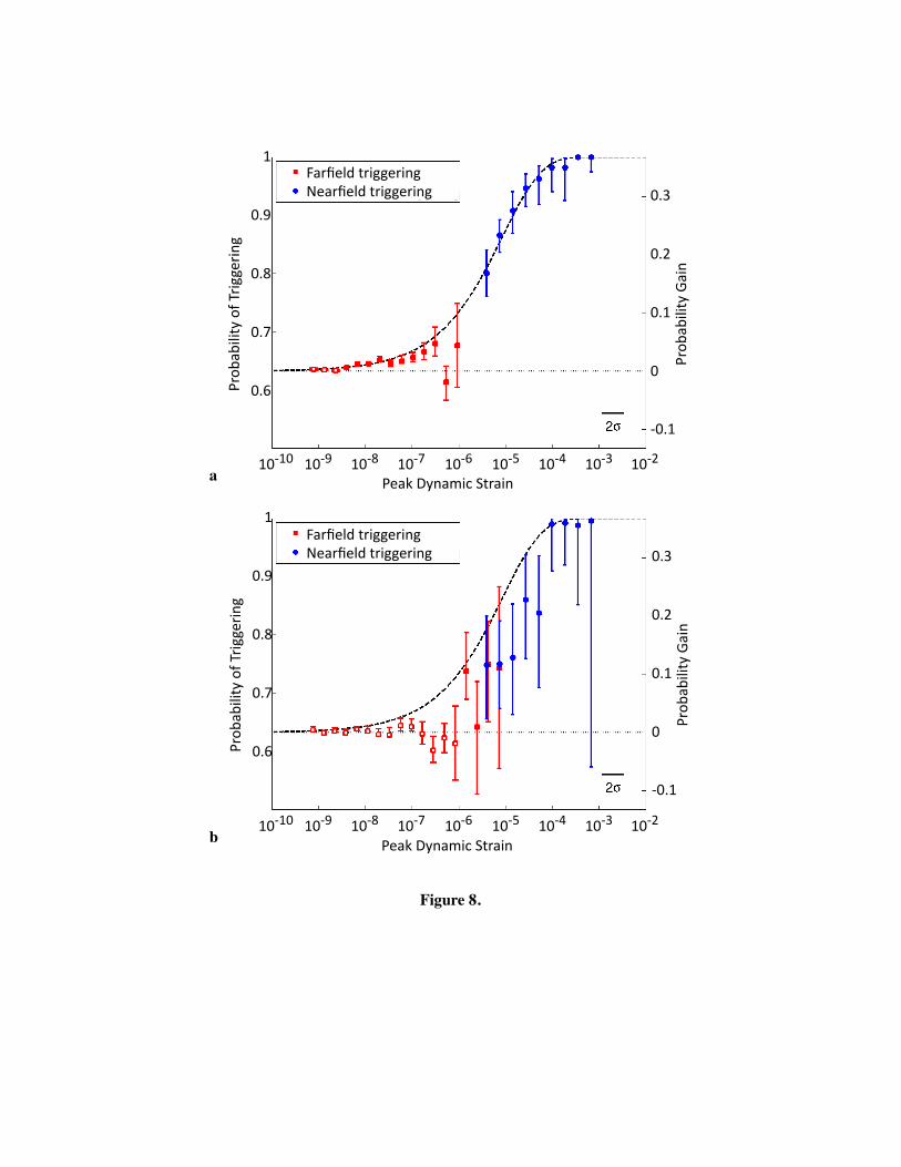
Figure 8.
PeakDynamicStrain10‐10
b 10‐9 10‐8 10‐7 10‐6 10‐5 10‐4 10‐3 10‐2
FarfieldtriggeringNearfieldtriggering
PeakDynamicStrain10‐10
Prob
abilityofTriggering
a 10‐9 10‐8 10‐7 10‐6 10‐5 10‐4 10‐3 10‐2
0.6
FarfieldtriggeringNearfieldtriggering
0.7
0.8
0.9
1
‐0.1
Prob
abilityGain
0
0.1
0.2
0.3
Prob
abilityofTriggering
0.6
0.7
0.8
0.9
1
‐0.1
Prob
abilityGain
0
0.1
0.2
0.3

Figure 9.
Magnitude2
TriggeringIntensity
3 4 5 6 710‐2
10‐1
100
103
104
101
102
8

PeakDynamicStrain10‐10
10‐3
TriggeringIntensity
a 10‐9 10‐8 10‐7 10‐6 10‐5 10‐4 10‐3 10‐2
10‐2
10‐1
100
101
102
PeakDynamicStrain10‐10
10‐3
TriggeringIntensity
b
10‐9 10‐8 10‐7 10‐6 10‐5 10‐4 10‐3 10‐2
10‐2
10‐1
100
101
102
PeakDynamicStrain10‐10
10‐3
TriggeringIntensity
c 10‐9 10‐8 10‐7 10‐6 10‐5 10‐4 10‐3 10‐2
10‐2
10‐1
100
101
102
BackgroundFrac1oninCatalog0.1
0.4
RecoveredSlop
e
d
Simula1on:Hardebeck Simula1on:Console
Simula1on:Reasenberg
0.5
0.6
0.7
0.8
0.9
1
0.2 0.3 0.4 0.5 0.6 0.7
Figure 10.

TotalDynamicStrain
10‐3
TriggeringIntensity
10‐9 10‐8 10‐7 10‐6 10‐5 10‐4 10‐3 10‐2
10‐2
10‐1
100
101
102
10‐1 100
Figure 12.
PeakDynamicStrain
10‐3
TriggeringIntensity
10‐2
10‐1
100
10‐10 10‐8 10‐7 10‐6 10‐510‐9
Figure 11.
800km1600km3200km
0.025°0.05°0.1°
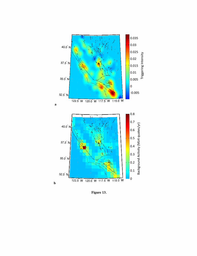
TriggeringIntensity
0.03
Figure 13.
0.02
0.01
0
0.035
0.025
0.015
0.005
‐0.005
b
a
Backgrou
ndAc1vity(M
≥4quakes/yr)0.7
0.8
0.6
0.5
0.4
0.3
0.2
0.1
0