conjoint sas
TRANSCRIPT
SAS Technical Report R-l 09Conjoint Analysis Examples
SAS Institute Inc.SAS Campus DriveCaty, NC 2751:3

The correct bibliographic citation for this manual is as follows: SAS Institute Inc.,SAS*Teclmical Report R-109, Conjoint Analysis Examples, Gary, NC: SAS Institute Inc.,1993.85 pp.
SAS@Technical Report R-109, Conjoint Analysis Examples
Copyright ’ 1993 by SAS Institute Inc., Cary, NC, USA.
ISBN 1-55544-581-O
All rights reserved. Printed in the United States of America. No part of this publication maybe reproduced, stored in a retrieval system, or transmitted, in any form or by any means,electronic, mechanical, photocopying, or otherwise, without the prior written permission ofthe publisher, SAS Institute Inc.
1st printing, September 1993
The SAS”System is an integrated system of software providing complete control over dataaccess, management, analysis, and presentation. Base SAS software is the foundation of theSAS System. Products within the SAS System include SAS/ACCESST SAS/wSAS/ASSIST SASKALC SASKONNBCT SASKPE: SAS/DMI: SAS/EIStSAS/ENGLISw SAS/ETSf SAS/.PSe SAS/GRAPw SAS/IML: SAS/IMS-DLRSAS/INSIGm SAS/LABt SAS/OR; SAS/PH-Clinic@ SAS/QCf SASKEPLAY-CICSPSAS/SHARl$ SAS/STATP SAS/TOOLIUy SAS/TUTOe SAS/DB2; SAS/GIS;SAS/IMAGE; SAS/NVISION; SAS/SESSION; and SAS/SQL-DS” software. Other SASInstitute products are SYSTEM 2000@ Data Management Software, with basic SYSTEM2000, CREATE; Multi-User; QueX, Screen Writer; and CICS interface software;NeoVisuaIs@ software; JMK IMP IN: IMP Serve: and IMP Design@ software;SAS/RTERM@ software; and the SASK? Compiler and the SAS/CX@Compiler; and Emulus”software. MultiVendor Architecture” and MVA” are trademarks of SAS Institute Inc. SASVideo Productions” and the SVP logo are service marks of SAS Institute Inc. SAS Institutealso offers SAS Consultingf Ambassador Select” and On-Site Ambassador= services.Authorline Observatioruf SAS Communicationsf SAS Training: SAS Viewsf’ the SASwareBallot and JMPer Cable- are published by SAS Institute Inc. All trademarks above areregistered trademarks or trademarks of SAS Institute Inc. in the USA and other countries. @indicates USA registration.
The Institute is a private company devoted to the support and further development of itssoftware and related services.
Other brand and product names are registered trademarks or trademarks of their respectivecompanies.

Table of Contents
Conjoint Analysis Examples . . . . . . . . . . . . . . . . . . . . . . . . . . . . . . . . . . . . . . . . . . . .Overview . . . . . . . . . . . . . . . . . . . . . . . . . . . . . . . . . . . . . . . . . . . . . . . . . . . . . . .
Conjoint Measurement . . . . . . . . . . . . . . . . . . . . . . . . . . . . . . . . . . . . . . . . . . .Conjoint Analysis . . . . . . . . . . . . . . . . . . . . . . . . . . . . . . . . . . . . . . . . . . . . . . .Simulating Market Share . . . . . . . . . . . . . . . . . . . . . . . . . . . . . . . . . . . . . . . . .Design of Experiments . . . . . . . . . . . . . . . . . . . . . . . . . . . . . . . . . . . . . . . . . . .
Example 1. Chocolate Candy . . . . . . . . . . . . . . . . . . . . . . . . . . . . . . . . . . . . .Metric Conjoint Analysis . . . . . . . . . . . . . . . . . . . . . . . . . . . . . . . . . . . . . . . . .
Output 1.1. Metric Conjoint Analysis . . . . . . . . . . . . . . . . . . . . . . . . . . . . .Nonmetric Conjoint Analysis . . . . . . . . . . . . . . . . . . . . . . . . . . . . . . . . . . . . . .
Output 1.2. Nonmetric Conjoint Analysis . . . . . . . . . . . . . . . . . . . . . . . . . .Example 2. Tea Tasting (Basic) . . . . . . . . . . . . . . . . . . . . . . . . . . . . . . . . . . . .
Metric Conjoint Analysis . . . . . . . . . . . . . . . . . . . . . . . . . . . . . . . . . . . . . . . . .Output 2.1. Metric Conjoint Analysis . . . . . . . . . . . . . . . . . . . . . . . . . . . . .
Example 3. Tea Tasting (Advanced) . . . . . . . . . . . . . . . . . . . . . . . . . . . . . . .Creating a Design Matrix with ADX . . . . . . . . . . . . . . . . . . . . . . . . . . . . . . . . .Adding Labels, Formats, and Holdouts . . . . . . . . . . . . . . . . . . . . . . . . . . . . . . .
Output 3.1. Design Matrix with Labels and Formats . . . . . . . . . . . . . . . . . .Output 3.2. Design Matrix with Holdouts . . . . . . . . . . . . . . . . . . . . . . . . . .
PrinttheStimuli . . . . . . . . . . . . . . . . . . . . . . . . . . . . . . . . . . . . . . . . . . . . . . . .Output 3.3. The First Two Stimuli for the Conjoint Study . . . . . . . . . . . . .
Data Collection, Entry, and Preprocessing . . . . . . . . . . . . . . . . . . . . . . . . . . . .Output 3.4. Data and Design Together . . . . . . . . . . . . . . . . . . . . . . . . . . . .Output3.5. ASubsetoftheFinalInputDataSet . . . . . . . . . . . . . . . . . . . .
Metric Conjoint Analysis . . . . . . . . . . . . . . . . . . . . . . . . . . . . . . . . . . . . . . . . .Output 3.6. Metric Conjoint Analysis . . . . . . . . . . . . . . . . . . . . . . . . . . . . .Output 3.7. Predicted Utilities . . . . . . . . . . . . . . . . . . . . . . . . . . . . . . . . . .Output 3.8. Holdout Validation Results . . . . . . . . . . . . . . . . . . . . . . . . . . .Output 3.9. Simulation Results . . . . . . . . . . . . . . . . . . . . . . . . . . . . . . . . . .
Summarizing Results Across Subjects . . . . . . . . . . . . . . . . . . . . . . . . . . . . . . .Output 3.10. OUTTEST= Data Set Contents . . . . . . . . . . . . . . . . . . . . . . .Output 3.11. Individual R-Squares . . . . . . . . . . . . . . . . . . . . . . . . . . . . . . .Output 3.12. Conjoint Analysis Summary Statistics . . . . . . . . . . . . . . . . . .
Example 4. Spaghetti Sauce . . . . . . . . . . . . . . . . . . . . . . . . . . . . . . . . . . . . . .Create a Nonorthogonal Design Matrix with PROC OPTEX . . . . . . . . . . . . . . .
Output 4.1. Experimental Design Creation (First Ten) . . . . . . . . . . . . . . . .Output 4.2. Experimental Design . . . . . . . . . . . . . . . . . . . . . . . . . . . . . . . .
Generate Descriptions of the Sauces . . . . . . . . . . . . . . . . . . . . . . . . . . . . . . . . .Prepare For Data Collection with PROC FSEDIT . . . . . . . . . . . . . . . . . . . . . . .Collecting Data Using PROC FSEDIT . . . . . . . . . . . . . . . . . . . . . . . . . . . . . . .
1112335569
101213141616181921212222232424252829303131323333343637394043
Tab/e of Contents q q q iv
Output 4.3. Conjoint Input Data . . . . . . . . . . . . . . . . . . . . . . . . . . . . . . . . . 45Metric Conjoint Analysis . . . . . . . . . . . . . . . . . . . . . . . . . . . . . . . . . . . . . . . . . 46
Output 4.4. Metric Conjoint Analysis . . . . . . . . . . . . . . . . . . . . . . . . . . . . . 47Simulating Market Share, Maximum Utility Model . . . . . . . . . . . . . . . . . . . . . 50
Output 4.5. Market Share Simulation . . . . . . . . . . . . . . . . . . . . . . . . . . . . . 53Simulating Market Share, Bradley-Terry-Lute and Logit Models . . . . . . . . . . . 54
Output 4.6. Market Share Simulation . . . . . . . . . . . . . . . . . . . . . . . . . . . . . 55SimulatorComparisons . . . . . . . . . . . . . . . . . . . . . . . . . . . . . . . . . . . . . . . . ..5 6Change in Market Share . . . . . . . . . . . . . . . . . . . . . . . . . . . . . . . . . . . . . . . . . . 59
Output 4.7. Effects of New Products . . . . . . . . . . . . . . . . . . . . . . . . . . . . . 60Output 4.8. Change in Market Share . . . . . . . . . . . . . . . . . . . . . . . . . . . . . 62
Brand by Price Interactions . . . . . . . . . . . . . . . . . . . . . . . . . . . . . . . . . . . . . . . . 62Example 5. Choice of Chocolate Candies . . . . . . . . . . . . . . . . . . . . . . . . . . 64
Multinomial Logit Model . . . . . . . . . . . . . . . . . . . . . . . . . . . . . . . . . . . . . . . . . 65Output 5.1. Multinomial Logit Model with Chocolate Data . . . . . . . . . . . . 66Output 5.2. Multinomial Logit Model with Chocolate Data . . . . . . . . . . . . 68
PROC TRANSREG Specifications . . . . . . . . . . . . . . . . . . . . . . . . . . . . . . . . . 69PROC TRANSREG Statement . . . . . . . . . . . . . . . . . . . . . . . . . . . . . . . . . . . . . 69AlgorithmOptions . . . . . . . . . . . . . . . . . . . . . . . . . . . . . . . . . . . . . . . . . . . . . . 70OutputOptions . . . . . . . . . . . . . . . . . . . . . . . . . . . . . . . . . . . . . . . . . . . . . . . . . 72Transformations and Expansions . . . . . . . . . . . . . . . . . . . . . . . . . . . . . . . . . . . 72Transformation Options . . . . . . . . . . . . . . . . . . . . . . . . . . . . . . . . . . . . . . . . . . 74BYStatement . . . . . . . . . . . . . . . . . . . . . . . . . . . . . . . . . . . . . . . . . . . . . . . . . . 75IDStatement . . . . . . . . . . . . . . . . . . . . . . . . . . . . . . . . . . . . . . . . . . . . . . . . . . 76WEIGHTStatement . . . . . . . . . . . . . . . . . . . . . . . . . . . . . . . . . . . . . . . . . . . . . 76
Samples of PROC TRANSREG Usage . . . . . . . . . . . . . . . . . . . . . . . . . . . . . . 77Metric Conjoint Analysis with Rank-Order Data . . . . . . . . . . . . . . . . . . . . . . . . 77Metric Conjoint Analysis with Rating Scale Data . . . . . . . . . . . . . . . . . . . . . . . 77Nonmetric Conjoint Analysis . . . . . . . . . . . . . . . . . . . . . . . . . . . . . . . . . . . . . . 78MonotoneSplines . . . . . . . . . . . . . . . . . . . . . . . . . . . . . . . . . . . . . . . . . . . . . . . 78Constraints on the Utilities . . . . . . . . . . . . . . . . . . . . . . . . . . . . . . . . . . . . . . . . 78A Discontinuous Price Function . . . . . . . . . . . . . . . . . . . . . . . . . . . . . . . . . . . . 79MoreThanOneSubject . . . . . . . . . . . . . . . . . . . . . . . . . . . . . . . . . . . . . . . . . . 79
References . . . . . . . . . . . . . . . . . . . . . . . . . . . . . . . . . . . . . . . . . . . . . . . . . . . . . 80
Index ._............................................_............__. 81

Credits
SAS Technical Report R-109 was created and written by Warren F. Kuhfeld. Developmentand support of the TRANSREJG procedure is the responsibility of Warren F. Kuhfeld.

Conjoint Analysis Examples
OverviewConjoint analysis is used to analyze product preference data and simulate consumerchoice. This report describes conjoint analysis and provides examples using the SASSystem. Topics includemetric andnonmetricconjointanalysis, orthogonal andnonorthogonal experimental designs, data collection and manipulation, holdouts,brand by price interactions, maximum utility and multinomial logit simulators, andchange in market share. In addition, the multinomial logit model for discrete choicedata is briefly discussed.
Conjoint analysis is also used to study the factors that influence consumers’ purchas-ing decisions. Products possess attributes such as price, color, guarantee, environ-mental impact, predicted reliability, and so on. Consumers typically do not have theoption of buying the product that is best in every attribute, particularly when one ofthoseattributesisprice. Consumersareforcedtomaketrade-offs as they decidewhich products to purchase. Consider the decision to purchase a car. Increased sizegenerally means increased safety and comfort, whichmust be tradedoff with in-creased cost and pollution. Conjoint analysis is used to study these trade-offs.
Conjoint analysis is a popular marketing research technique. It is used in designingnew products, changing or repositioning existing products, evaluating the effects ofprice on purchase intent, and simulating market share. Refer to Green and Rao (197 1)and Green and Wind (1975) for early introductions to conjoint analysis, refer to Lou-viere (1988) for a more recent introduction, and refer to Green and Srinivasan (1990)for a recent review article.
Conjoint Measurement
Conjoint analysis grew out of the area of conjoint measurement in mathematical psy-chology. Conjoint measurement is used to investigate the joint effect of a set of inde-pendent variables on an ordinal-scale-of-measurement dependent variable. The inde-pendent variables are typically nominal and sometimes interval-scaled variables.Conjoint measurement simultaneously finds a monotonic scoring of the dependentvariable and numerical values for each level of each independent variable. The goalis to monotonically transform the ordinal values to equal the sum of their attributelevel values. Hence, conjoint measurement is used to derive an interval variable fromordinal data. The conjoint measurement model is a mathematical model, not a statisti-cal model, since it has no statistical error term.
2 q q q Conjoint Analysis Examples
Conjoint Analysis
Conjoint anaZysis is based on a main effects analysis-of-variance model. Data arecollected by asking subjects about their preferences for hypothetical products definedby attribute combinations. Conjoint analysis decomposes the judgment data intocomponents, based on qualitative attributes of the products. A numerical utility orpart-worth utility value is computed for each level of each attribute. Large utilitiesare assigned to the most preferred levels, and small utilities are assigned to the leastpreferred levels. The attributes with the largest utility range are considered the mostimportant in predicting preference. Conjoint analysis is a statistical model with anerror term and a loss function.
Metric conjoint analysis models the judgments directly. When all of the attributesare nominal, the metric conjoint analysis is a simple main-effects ANOVA with somespecialized output. The attributes are the independent variables, the judgments com-prise the dependent variable, and the utilities are the parameter estimates from theANOVA model. The following is a metric conjoint analysis model for three factors.
Yijk = p + hi + k?j + p3k + %jk
where
This model could be used, for example, to investigate preferences for cars that differon three attributes: mileage, expected reliability, and price. y$ is one subject’s statedpreference for a car with the ith level of mileage, the jth level of expected reliability,and the k th level of price. The grand mean is ,u, and the error is E$.
Nonmetric conjoint analysis finds a monotonic transformation of the preference judg-ments. The model, which follows directly from conjoint measurement, iterativelyfits the ANOVA model until the transformation stabilizes. The R2 increases duringevery iteration until convergence, when the change in R2 is essentially zero. Thefollowing is a metric conjoint analysis model for three factors.
@(yjjk) = p + bli + 182j + r63k + ‘ijk
where a( y$ ) designates a monotonic transformation of the variable Y.
The R2 for a nonmetric conjoint analysis model will always be greater than or equalto the R2 from a metric analysis of the same data. The smaller R2 in metric conjointanalysis is not necessarily a disadvantage, since results should be more stable andreproducible with the metric model. Metric conjoint analysis was derived from non-metric conjoint analysis as a special case. Today, metric conjoint analysis is used
Conjoint Analysis q q q 3
more often than nonmetric conjoint analysis.
In the SAS System, conjoint analysis is performed with the SAS/STAT procedureTRANSREG (transformation regression). Metric conjoint analysis models are fit us-ing ordinary least squares, and nonmetric conjoint analysis models are fit using analternating least squares algorithm (Young, 1981; Gifi, 1990). Conjoint analysis isexplained more fully in the examples. The “PROC TRANSREG Specifications” sec-tion of this technical report documents the PROC TRANSREG statements and op-tions that are most relevant to conjoint analysis. The “Samples of PROCTRANSREG Usage” section shows some typical conjoint analysis specifications.
Simulating Market Share
In many conjoint analysis studies, the conjoint analysis is not the primary goal. Theconjoint analysis is used to generate utilities, which are thenused as input to consumerchoice and market share simulators. The end result for a product is its expected mar-ket share, which is a prediction of the proportion of times that the product will bepurchased. The effects on market share of introducing new products can also be simu-lated.
One of the most popular ways to simulate market share is with the maximum utilitymodel, which assumes each subject will buy with probability 1 .O the product forwhich he or she has the highest utility. The probabilities for each product are aver-aged across subjects to get predicted market share.
Other simulation methods include the Bradley-Terry-Lute (BTL) model and the logitmodel. In the BTL model, probability of choice is a linear function of utility. Inthe logit model, probability is a logit function of utility. The logit function is nonlin-ear and strictly increasing.
Maximum Utility: Pijk = 1.0 if yijk = MAx( yik), otherwise p;jk = 0.0
BTL: pijk = Yijk 12 Yijk
Logit:
Design of Experiments
The design of experiments is a fundamental part of conjoint anillysis. During conjointanalysis data collection, subjects are asked to judge their preferences for hypotheticalproducts defined by attribute combinations, Experimental designs are used to selectattribute combinations. The factors of an experimental design are variables that havetwo or more fixed values, or levels. Experiments are performed to study the effectsof the factor levels on the response, or dependent variable. In a conjoint study, thefactors are the attributes of the hypotheticaI products or services, and the responseis preference or choice.
The simplest experimental design to generate is the full-factorial design, which con-sists of all possible combinations of the levels of the factors. With five factors, twowith two levels, and three with three levels, denoted 2233, there are 108 possible
4 q q q Conjoint Analysis Examples
combinations. In a full-factorial design, all main effects, all two-way interactions,and all higher-order interactions are estimable. The problem with a full-factorial de-sign is that, for most practical problems, it is too difficult for subjects to rate all possi-ble combinations.
For this reason, researchers often use fractional-factorial designs, which consist offewer runs (factor level combinations) than full-factorial designs. The problem withhaving fewer runs is that some effects become confounded. Two effects are said tobe confounded or aliased when their effects cannot be distinguished from each otherbecause the levels they take in the design yield identical partitions of the runs.
A special type of fractional-factorial design is the orthogonal array, in which all es-timable effects are uncorrelated. Orthogonal arrays for main-effects models are fre-quently used in marketing research. Orthogonal designs are often practical for main-effects models when the number of factors is small (say six or fewer) and the numberof levels of each factor is small (say four or fewer). You should use an orthogonaldesign whenever possible. However, there are some situations in which orthogonaldesigns are not practical, such as when
l not all combinations of factor levels are feasible or make sense
l the desired number of runs is not available in an orthogonal design
l a nonstandard model is being used, such as a model with interactions, polynomials,or splines.
When an orthogonal design is not practical, you must make a choice. One choice isto change the factors and levels to fit some known orthogonal design. This choiceis undesirable for obvious reasons. When a suitable orthogonal design does not exist,nonorthogonal designs can be used instead. Nonorthogonal designs, where some co-efficients may be slightly correlated, can be used in all of the situations listed previ-ously. You do not have to adapt every experiment to fit some known orthogonal ar-ray. First you choose the number of runs. You are not restricted by the sizes of or-thogonal arrays, which come in specific numbers of runs (such as 16,18,27,32,36,and so forth) for specific numbers of factors with specific numbers of levels. Thenyou choose a set of candidutepoints, which may be all of the points in a full-factorialdesign or they may be a subset, excluding unrealistic combinations. Algorithms forgenerating nonorthogonal designs select a set of design points, from the candidatepoints, that optimize an efficiency criterion.
Measures of the efficiency of an (N u ⌧ p> rdesign matrix X are based on the informu-tion matrix X ’ X and its inverse (X ’ X) . The variance-covariance matrix of thevector o_fiparameter estimates /? in a least-squares analysis is proportional to( x ’x ) . An efficient design will have a “small” variance matrix; variance andefficiency are inversely related. The eigenvalues of (X ’ X) -I provide measures ofthe “size” of the variance matrix. A-eficiency is a_unction of the arithmetic meanof the eigenvalues, which is given by trace( (X ’ X) ) / p. D-efSiciency is a function
of the geometric mean of the eigenvalues, which is given by 1 (X ’ X) -’ 1 I”. If anorthogonal design exists, then it has optimum efficiency; conversely, the more effi-cient a design is, the more it tends toward orthogonality. The measures of efficiencycan be scaled to range from 0 to 100, as shown in the following.
Design of Experiments q q 0 5
A-efficiency = 100 X 1N+z((X'X)-')/p
D-efficiency = 100 x 1N, 1 (X’X) -’ 1 “’
These efficiencies measure the goodness of the design relative to orthogonal designsthat may be far from possible, so they are not useful as absolute measures of designefficiency. Instead, they should be used relatively, to compare one design to anotherfor the same situation.
The ADX menu system of SAS/QC software can be used to generate an orthogonalarray experimental design. The SAS/QC procedure OPTEX can be used to findnonorthogonal designs. See Example 3 for an illustration of using ADX to generatean orthogonal array, and see Example 4 for an illustration of using PROC OPTEX.Refer to Kuhfeld, Garratt, and Tobias (1993) for more information on nonorthogonalexperimental designs.
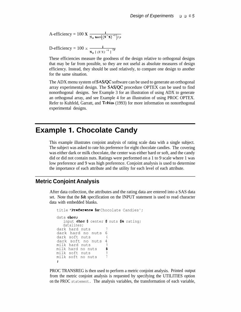
Example 1. Chocolate CandyThis example illustrates conjoint analysis of rating scale data with a single subject.The subject was asked to rate his preference for eight chocolate candies. The coveringwas either dark or milk chocolate, the center was either hard or soft, and the candydid or did not contain nuts. Ratings were performed on a 1 to 9 scale where 1 waslow preference and 9 was high preference. Conjoint analysis is used to determinethe importance of each attribute and the utility for each level of each attribute.
Metric Conjoint Analysis
After data collection, the attributes and the rating data are entered into a SAS dataset. Note that the $8~ specification on the INPUT statement is used to read characterdata with embedded blanks.
title ',Preference for Chocolate Candies';
data choc;input cboc $ center $ nuts $6( rating;datalines;
dark hard nuts 7dark hard no nuts 6dark soft nuts 6dark soft no nuts 4milk hard nuts 9milk hard no nuts 8milk soft nuts 9milk soft no nuts 7;
PROC TRANSREG is then used to perform a metric conjoint analysis. Printed outputfrom the metric conjoint analysis is requested by specifying the UTILITIES optionon the PROC statement. The analysis variables, the transformation of each variable,
6 q q q Conjoint Analysis Examples
and transformation specific options are specified on the MODEL statement.
proc transreg utilities;title2 'Metric Conjoint Analysis';model lineartrating) = class(choc center nuts / zero=sum);run:
The MODEL statement provides a syntax for general transformation regression mod-els, so it is markedly different from other SAS/STAT procedure MODEL statements.Variable lists are specified in parentheses after a transformation name,LINEAR(RATING) requests a LINEAR transformation of the dependent variableRATING. A transformation name must be specified for all variable lists, even forthe dependent variable in metric conjoint analysis, when no transformation is desired.The linear transformation of RATING will not change the original scoring. An equalsign follows the dependent variable specification, then the attribute variables arespecified along with their transformation.
class(choc center nuts / zero=sum)
designates the attributes as CLASS variables with the restriction that the utilities sumto zero within each attribute. A slash must be specified to separate the variables fromthe transformation option ZERO=SUM. CLASS creates amain-effects design matrixfrom the specified variables. This example produces only printed output; later exam-ples will show how to store results in output SAS data sets.
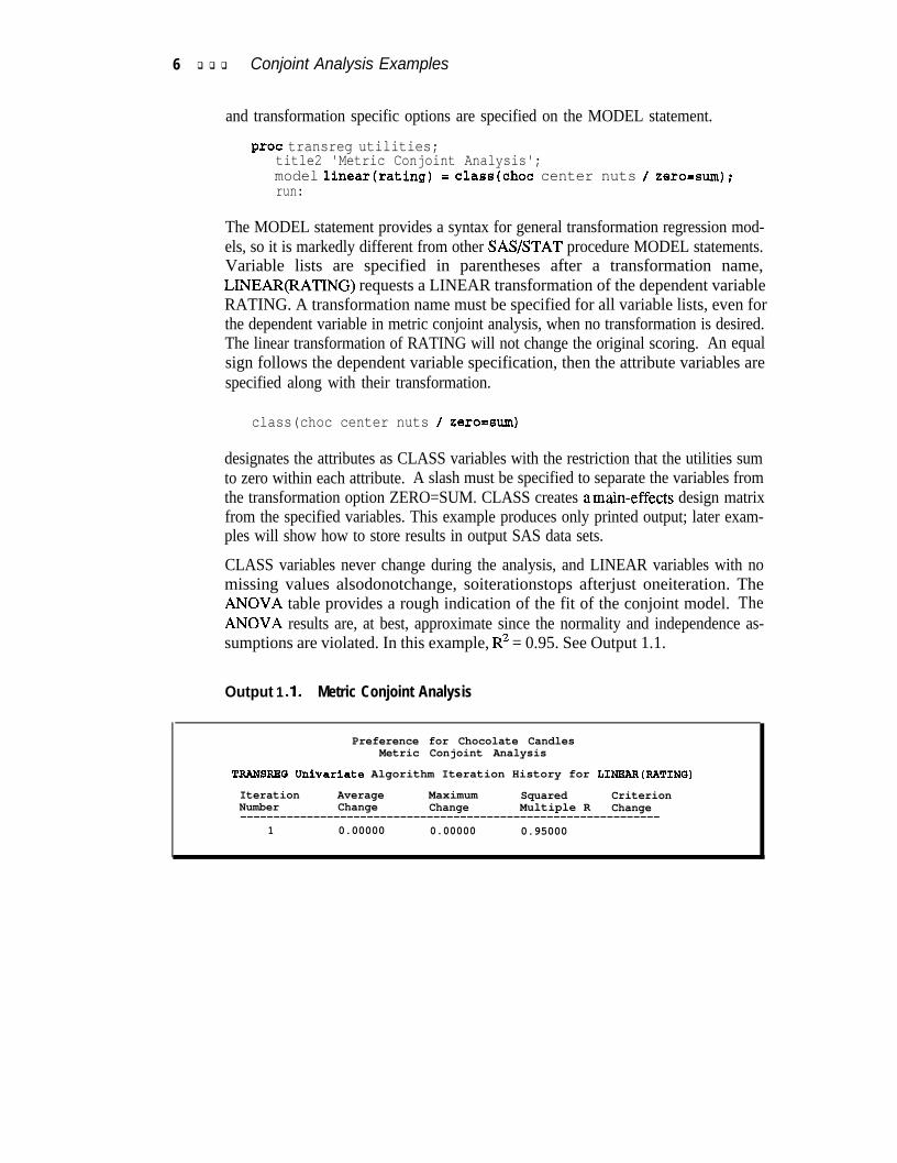
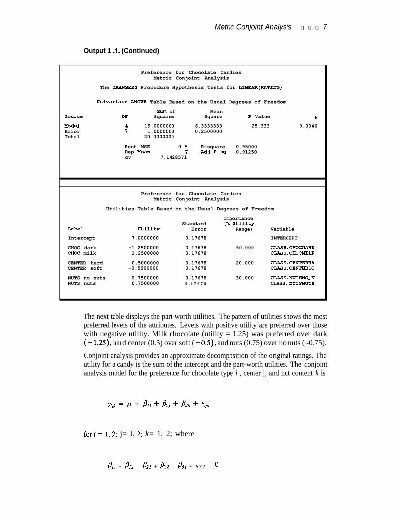
CLASS variables never change during the analysis, and LINEAR variables with nomissing values alsodonotchange, soiterationstops afterjust oneiteration. TheANOVA table provides a rough indication of the fit of the conjoint model. TheANOVA results are, at best, approximate since the normality and independence as-sumptions are violated. In this example, R2 = 0.95. See Output 1.1.
Output 1 .I. Metric Conjoint Analysis
Preference for Chocolate CandlesMetric Conjoint Analysis
TRANSREQ Univariate Algorithm Iteration History for LINEAR(RATIN0)
Iteration Average Maximum Squared CriterionNumber Change Change Multiple R Change---------------------------------------------------------------
1 0.00000 0.00000 0.95000
Metric Conjoint Analysis q q q 7
Output 1 .l. (Continued)
Preference for Chocolate CandiesMetric Conjoint Analysis
The TRANSREQ Procedure Hypothesis Tests for LINBAR(RATINQ)
Univariate ANOVA Table Based on the Usual Degrees of Freedom
Source
NOddErrorTotal
suln of MeanDF Squares Square F Value P
3 19.0000000 6.3333333 25.333 0.00467" 1.0000000 0.2500000
20.0000000
Root MSE 0.5 R-square 0.95000Dep Mean I Adj R-q 0.91250cv 7.1428571
Preference for Chocolate CandiesMetric Conjoint Analysis
Utilities Table Based on the Usual Degrees of Freedom
Label Utility
Intercept 7.0000000
CHOC dark -1.2500000CHOC milk 1.2500000
CENTER hard 0.5000000CENTER soft -0.5000000
NUTS no nuts -0.7500000NUTS nuts 0.7500000
StandardError
0.17678
0.176780.17678
0.176780.17678
0.176780 . 1 7 6 7 8
Importance(96 Utility
Range)
50.000
20.000
30.000
Variable
INTERCEPT
CLAsS.CHOCDARKCLASS.CHOCYILK
CLAsS.CENTERHACLASS.CENTERSO
CLASS.NUTSNO-NCLASS. NUTSNUTS
The next table displays the part-worth utilities. The pattern of utilities shows the mostpreferred levels of the attributes. Levels with positive utility are preferred over thosewith negative utility. Milk chocolate (utility = 1.25) was preferred over dark(- 1.25)) hard center (0.5) over soft ( -0.5), and nuts (0.75) over no nuts ( -0.75).
Conjoint analysis provides an approximate decomposition of the original ratings. Theutility for a candy is the sum of the intercept and the part-worth utilities. The conjointanalysis model for the preference for chocolate type i , center j, and nut content k is
y$ = p + bli + 182j ’ b3k + ‘ijk
fori= 1,2; j= 1,2; k= 1, 2; where
&, + n’%2 = p21 + i’% = 1831 + 8 3 2 = o
8 q q q Conjoint Analysis Examples
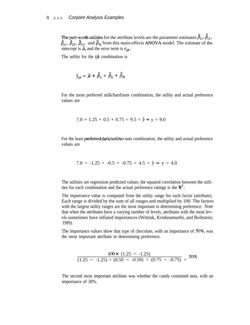
Fe hart-yorth utiliiies for the attribute levels are the parameter estimates j,,, &,& I% 1831, and & from this main-effects ANOVA model. The estimate of theintercept is I;;, and the error term is E+.
The utility for the ijk combination is
Yi$ = I; + b,i + t%j + 63k
For the most preferred milk/hard/nuts combination, the utility and actual preferencevalues are
7.0 + 1.25 + 0.5 + 0.75 = 9.5 = 5 = y = 9.0
For the least preferreddark/soft/no nuts combination, the utility and actual preferencevalues are
7.0 + -1.25 + -0.5 + -0.75 = 4.5 = F = y = 4.0
The utilities are regression predicted values; the squared correlation between the utili-ties for each combination and the actual preference ratings is the R2.
The importance value is computed from the utility range for each factor (attribute).Each range is divided by the sum of all ranges and multiplied by 100. The factorswith the largest utility ranges are the most important in determining preference. Notethat when the attributes have a varying number of levels, attributes with the most lev-els sometimes have inflated importances (Wittink, Krishnamurthi, and Reibstein;1989).
The importance values show that type of chocolate, with an importance of 50%, wasthe most important attribute in determining preference.
100x (1.25 - -1.25)(1.25 - -1.25) + (0.50 - -0.50) + (0.75 - -0.75) = 50%
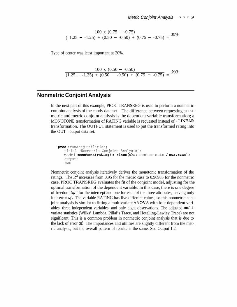
The second most important attribute was whether the candy contained nuts, with animportance of 30%.
Metric Conjoint Analysis 0 0 0 9
100 x (0.75 - -0.75)( 1.25 - -1.25) + (0.50 - -0.50) + (0.75 - -0.75) = 30%
Type of center was least important at 20%.
100 x (0.50 - -0.50)(1.25 - -1.25) + (0.50 - -0.50) + (0.75 - -0.75) = 20%
Nonmetric Conjoint Analysis
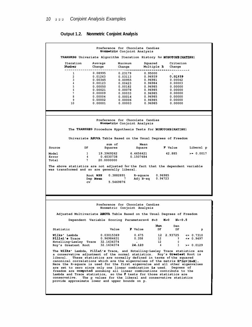
In the next part of this example, PROC TRANSREG is used to perform a nonmetricconjoint analysis of the candy data set. The difference between requesting a non-metric and metric conjoint analysis is the dependent variable transformation; aMONOTONE transformation of RATING variable is requested instead of aLINEARtransformation. The OUTPUT statement is used to put the transformed rating intothe OUT= output data set.
proc tranareg utilities;title2 ‘Nonmetric Conjoint Analysis’;model monotone(rating) = claaa(choc center nuts / zero=aum);output;run:
Nomnetric conjoint analysis iteratively derives the monotonic transformation of theratings. The R2 increases from 0.95 for the metric case to 0.96985 for the nonmetriccase. PROC TRANSREG evaluates the fit of the conjoint model, adjusting for theoptimal transformation of the dependent variable. In this case, there is one degreeof freedom (&) for the intercept and one for each of the three attributes, leaving onlyfour error df. The variable RATING has five different values, so this nonmetric con-joint analysis is similar to fitting a multivariate ANOVA with four dependent vari-ables, three independent variables, and only eight observations. The adjusted multi-variate statistics (Wilks’ Lambda, Pillai’s Trace, and Hotelling-Lawley Trace) are notsignificant. This is a common problem in nonmetric conjoint analysis that is due tothe lack of error df. The importances and utilities are slightly different from the met-ric analysis, but the overall pattern of results is the same. See Output 1.2.
10 q q q Conjoint Analysis Examples
Output 1.2. Nonmetric Conjoint Analysis
Preference for Chocolate CandiesNonmetric Conjoint Analysis
TRAWSRBG Univariate Algorithm Iteration History for MONOTONE(RATINQ)Iteration Average Maximum Squared CriterionNixnber Change Change Multiple R Change_-_________---__________________________-----------------------
1 0.08995 0.23179 0.950002 0.01263 0.03113 0.96939 0:019393 0.00345 0.00955 0.96981 0.000424 0.00123 0.00423 0.96984 0.000035 0.00050 0.00182 0.96985 0.000006 0.00021 0.00078 0.96985 0.000007 0.00009 0.00033 0.96985 0.000008 0.00004 0.00014 0.96985 0.000009 0.00002 0.00006 0.96985 0.00000
10 0.00001 0.00003 0.96985 0.00000
Preference for Chocolate CandiesNonmetric Conjoint Analysis
The TRANSRBQ Procedure Hypothesis Tests for YONOTONE(RATING)
Univariate ANOVA Table Based on the Usual Degrees of Freedom
sum of MeanSource DF Squares Square F Value Liberal p
Model 3 19.3969262 6.4656421 42.885 >= 0.0017Error 4 0.6030738 0.1507684Total 7 20.0000000
The above statistics are not adjusted for the fact that the dependent variablewas transformed and so are generally liberal.
Root YSE 0.3882891 R-square 0.96985Dep Mean 7 Adj B-sq 0.94723cv 5.5469876
Preference for Chocolate CandiesNonmetric Conjoint Analysis
Adjusted Multivariate ANOVA Table Based on the Usual Degrees of Freedom
Dependent Variable Scoring Parameters=4 S=3 M=O N=-0.5
Nun DenStatistic Value F Value DF DF P
Wilks' Lambda 0.03015369 0.675 12 2.93725 <= 0.7310Pillal's Trace 0.96984631 0.358 12 9 <= 0.9497Hotelling-Lawley Trace 32.1634374
24:12312 0
Roy's Greatest Root 32.1634374 4 3 ,= 0.0129
The Wilks' Lambda, Pillai‘s Trace, and Hotelling-Lawley Trace statistics area conservative adjustment of the normal statistics. Roy's Qreatest Root isliberal. These statistics are normally defined in terms of the squaredcanonical correlations which are the eigenvalues of the matrix H*inv(H+R).Here the R-square is used for the first eigenvalue and all other eigenvaluesare set to zero since only one linear combination is used. Degrees offreedom are computed assuming all linear combinations contribute to theLambda and Trace statistics, so the F tests for those statistics areconservative. The p values for the liberal and conservative statisticsprovide approximate lower and upper bounds on p.
Nonmetric Conjoint Analysis q q q 11
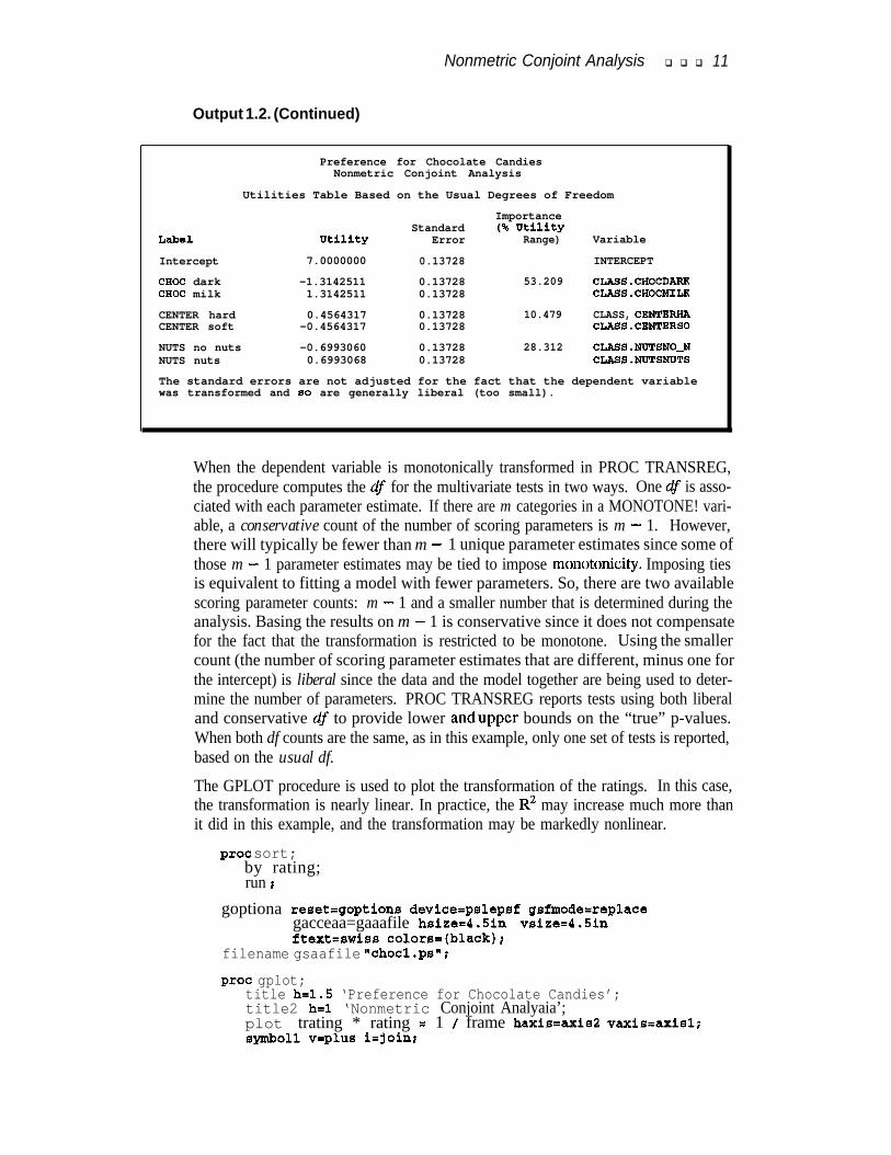
Output 1.2. (Continued)
Preference for Chocolate CandiesNonmetric Conjoint Analysis
Utilities Table Based on the Usual Degrees of Freedom
ImportanceStandard (% Utility
Label Utility Error Range) Variable
Intercept 7.0000000 0.13728 INTERCEPT
cHOC dark -1.3142511 0.13728 53.209 C!LASS.C!HOCDARXCHOC milk 1.3142511 0.13728 CLASS.CHOCMILK
CENTER hard 0.4564317 0.13728 10.479 CLASS, CENTERHACENTER soft -0.4564317 0.13728 CLASS.CENTERSO
NUTS no nuts -0.6993060 0.13728 28.312 CLASS.NUTSNO-NNUTS nuts 0.6993068 0.13728 CLASS.NUTSNDTS
The standard errors are not adjusted for the fact that the dependent variablewas transformed and so are generally liberal (too small).
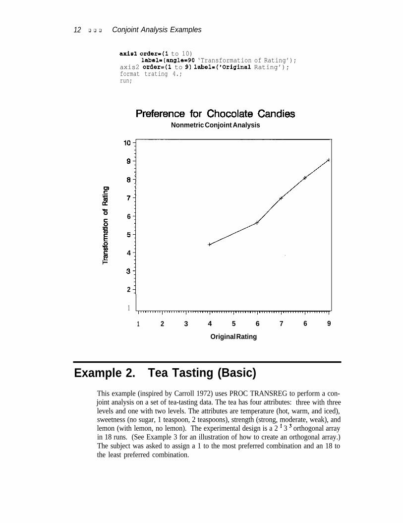
When the dependent variable is monotonically transformed in PROC TRANSREG,the procedure computes the df for the multivariate tests in two ways. One df is asso-ciated with each parameter estimate. If there are m categories in a MONOTONE! vari-able, a conservative count of the number of scoring parameters is m - 1. However,there will typically be fewer than m - 1 unique parameter estimates since some ofthose m - 1 parameter estimates may be tied to impose monotonic&y. Imposing tiesis equivalent to fitting a model with fewer parameters. So, there are two availablescoring parameter counts: m - 1 and a smaller number that is determined during theanalysis. Basing the results on m - 1 is conservative since it does not compensatefor the fact that the transformation is restricted to be monotone. Using the smallercount (the number of scoring parameter estimates that are different, minus one forthe intercept) is liberal since the data and the model together are being used to deter-mine the number of parameters. PROC TRANSREG reports tests using both liberaland conservative df to provide lower andupper bounds on the “true” p-values.When both df counts are the same, as in this example, only one set of tests is reported,based on the usual df.The GPLOT procedure is used to plot the transformation of the ratings. In this case,the transformation is nearly linear. In practice, the R2 may increase much more thanit did in this example, and the transformation may be markedly nonlinear.
proc sort;by rating;run ;
goptiona reaet=goptions device=palepaf gafmode-replacegacceaa=gaaafile haize4.5in vaize4.5inftext=awiaa colora=(black);
filename gsaafile “chocl.pa”;
proc gplot;title h4.5 ‘Preference for Chocolate Candies’;title2 h=l ‘Nonmetric Conjoint Analyaia’;plot trating * rating = 1 / frame haxia=axiaZ vaxia=axial;symbol1 v=plua i=join;
12 q q q Conjoint Analysis Examples
axis1 order=(l to 10)labek(anglex90 ‘Transformation of Rating’);
axis2 order=(l to 9) label=(‘Original Rating’);format trating 4.;run;
Preference for Chocolate CandiesNonmetric Conjoint Analysis
5E
6‘F;g 5B5 4I=
2
1
1 2 3 4 5 6 7 6 9
Original Rating
Example 2. Tea Tasting (Basic)This example (inspired by Carroll 1972) uses PROC TRANSREG to perform a con-joint analysis on a set of tea-tasting data. The tea has four attributes: three with threelevels and one with two levels. The attributes are temperature (hot, warm, and iced),sweetness (no sugar, 1 teaspoon, 2 teaspoons), strength (strong, moderate, weak), andlemon (with lemon, no lemon). The experimental design is a 2 r 3 3 orthogonal arrayin 18 runs. (See Example 3 for an illustration of how to create an orthogonal array.)The subject was asked to assign a 1 to the most preferred combination and an 18 tothe least preferred combination.
Metric Conjoint Analysis q q q 13
Metric Conjoint Analysis
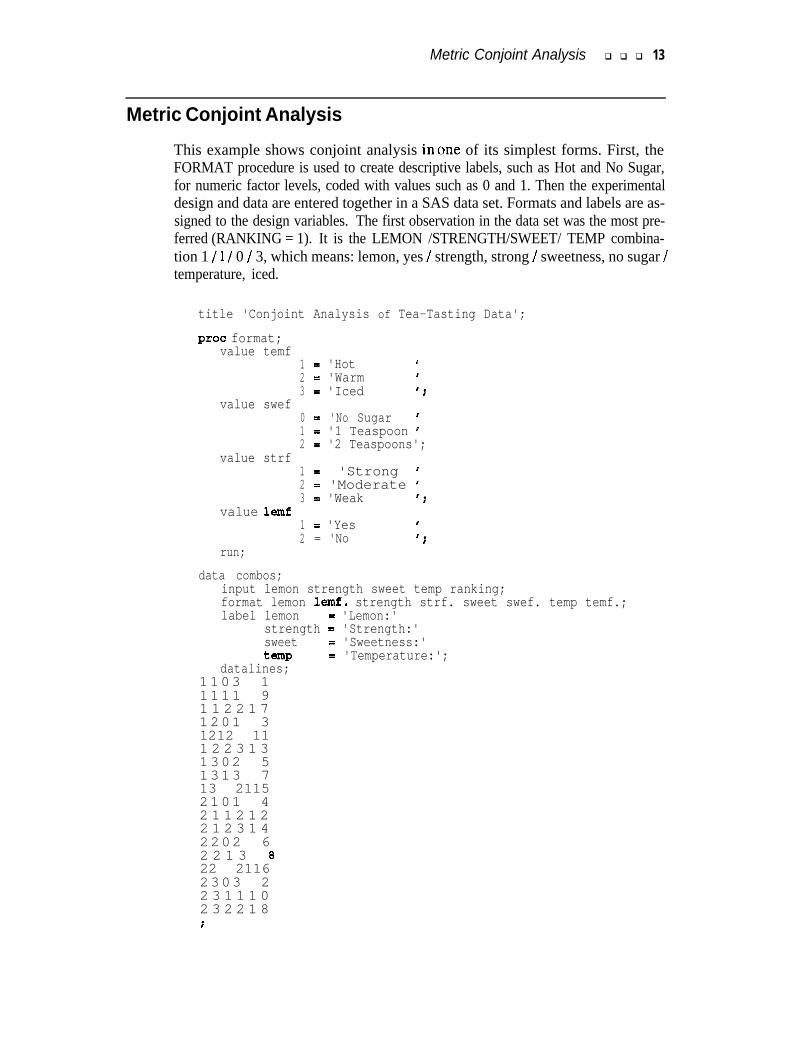
This example shows conjoint analysis inone of its simplest forms. First, theFORMAT procedure is used to create descriptive labels, such as Hot and No Sugar,for numeric factor levels, coded with values such as 0 and 1. Then the experimentaldesign and data are entered together in a SAS data set. Formats and labels are as-signed to the design variables. The first observation in the data set was the most pre-ferred (RANKING = 1). It is the LEMON /STRENGTH/SWEET/ TEMP combina-tion 1 / 1 / 0 / 3, which means: lemon, yes / strength, strong / sweetness, no sugar /temperature, iced.
title 'Conjoint Analysis of Tea-Tasting Data';
proc format;value temf
1 = 'Hot I2 = 'Warm I3 = 'Iced ';
value swef0 5: 'No Sugar '1 = '1 Teaspoon J2 = '2 Teaspoons';
value strf1 = 'Strong I2 = 'Moderate '3 = 'Weak ';
value lemf1 = 'Yes I2 = 'No ':
run;data combos;
input lemon strength sweet temp ranking;format lemon lemf. strength strf. sweet swef. temp temf.;label lemon = 'Lemon:'
strength = 'Strength:'sweet = 'Sweetness:'temp = 'Temperature:';
datalines;1103 11111 91 1 2 2 1 71201 31212 111 2 2 3 1 31302 51313 713 21152101 42 1 1 2 1 22 1 2 3 1 42202 62 2 1 3 822 21162303 22 3 1 1 1 02 3 2 2 1 8;
1 4 q q q Conjoint Analysis Examples
The UTILITIFS option on the PROC TRANSREG statement requests the conjointanalysis results. The SHORT option suppresses the iteration history tables, sincethere is only one iteration. The MODEL statement is like the earlier metric conjointanalysis MODEL statement: LINEAR is used for the dependent variable, and theattributes are designated as CLASS variables with the restriction that the utilities sumto zero within each attribute. The difference is that the REFLECT option is appliedto the dependent variable RANKING. A small rank means high preference, so thedata must be reflected so that high preference corresponds to a large utility. Withranksrangingfromlto18,REFLECTtransformslto18,2to17,...,rto(19-r),. . . . and 18 to 1.
The OUTPUT statement creates the OUT= data set, which contains the original vari-ables, transformed variables, and dummy variables. The utilities for each combina-tion are written to this data set by the DAPPROXIMATIONS option (for dependentvariable approximations, which are the predicted values). The IREPLACE optionspecifies that the transformed independent variables replace the original independentvariables, since both are the same.
Finally, the OUT= data set is sorted and the combinations are printed along with theirrank, transformed (reflected) rank, and rank approximation (predicted utility).
proc transreg utilities short;title2 'Use PROC TRANSREG to Perform the Conjoint Analysis';model linear(ranking / reflect) =
class(lemon temp sweet strength / zero=sum);output ireplace dapproximations;run:
proc sort;by ranking;run;
proc print;title2 'Some of the OUT= Data Set';var ranking tranking aranking lemon temp sweet strength;run;
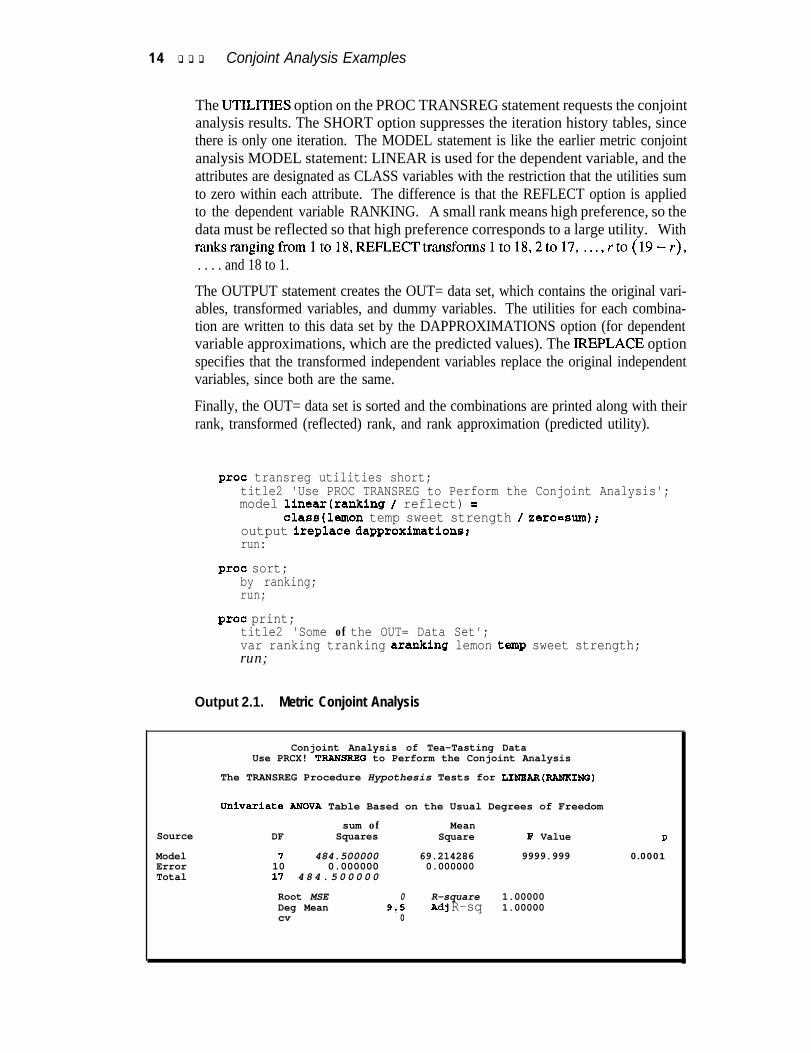
Output 2.1. Metric Conjoint Analysis
Conjoint Analysis of Tea-Tasting DataUse PRCX! TRANSREQ to Perform the Conjoint Analysis
The TRANSREG Procedure Hypothesis Tests for LINEAR(RANKINQ)
Univarlate ANOVA Table Based on the Usual Degrees of Freedom
Source
ModelErrorTotal
sum of MeanDF Squares Square F Value
7 484.500000 69.214286 9999.99910 0.000000 0.00000017 4 8 4 . 5 0 0 0 0 0
Root MSE 0 R-square 1.00000Deg Mean 9,5 Adj R-sq 1.00000cv 0
B0.0001
Metric Conjoint Analysis q q q 15
Output 2.1. (Continued)
Conjoint Analysis of Tea-Tasting DataUse PROC TRANSREQ to Perform the Conjoint Analysis
Utilities Table Based on the Usual Degrees of Freedom
Label Utility
Intercept 9.5000000
Lemon: NO -0.5000000Lelwn: Yes 0.5000000
Temperature: H o t - 0 . 0 0 0 0 0 0 0Temperature: I c e d 2 . 0 0 0 0 0 0 0Temperature: Warm -2.0000000
Sweetness: 1 Teaspoon 0.0000000Sweetness: 2 Teaspoons -6.0000000Sweetness: No Sugar 6.0000000
ImportanceStandard (% Utility
Error Range) Variable
0.0000 INTERCEPT
0.0000 5.882 cLASs.LEbfoNNo0.0000 CLASS.LEMONYES
0.0000 23.529 CLASS.TEbfPHOT0.0000 CLASS.TEMPICED0.0000 CLASS.TEMPWARM
0.0000 70.588 CLASS. SWBBTl-T0.0000 CLASS. SWBET2-T0.0000 CLASS.SWEETNO
Strength: Moderate 0.0000000 0.0000 0.000 CLASS. STRBNGMOStrength: Strong -0.0000000 0.0000 CLASS.STRBNGSTStrength: Weak 0.0000000 0.0000 CLASS.STRBNGWB
Conjoint Analysis of Tea-Tasting DataSome of the OUT= Data Set
OBS RANKING TRANKING APANKINQ LEMON TEMP SWBBT STRENGTH
1 1 18 18 Yes Iced No Sugar Strong2 2 17 17 No Iced No Sugar Weak3 3 16 16 Yes Hot No Sugar Moderate4 4 15 15 No Hot No Sugar Strong5 5 14 14 Yes Warm No Sugar Weak
7"6 137 12 ii
No Warm No Sugar ModerateYea Iced 1 Teaspoon Weak
8 8 11 11 No Iced 1 Teaspoon Moderate9 9 10 10 Yea Hot 1 Teaspoon Strong
10 10 9 9 No Hot 1 Teaspoon Weak11 11 8 8 Yes Warm 1 Teaspoon Moderate12 12 7 7 No Warm 1 Teaspoon Strong13 13 6 6 Yes Iced 2 Teaspoons Moderate14 14 5 5 No Iced 2 Teaspoons Strong15 15 4 4 Ye0 Hot 2 Teaspoons Weak16 16 3 3 No Hot 2 Teaspoons Moderate17 17 2 2 Yea Warm 2 Teaspoons Strong18 18 1 1 No Warm 2 Teaspoons Weak
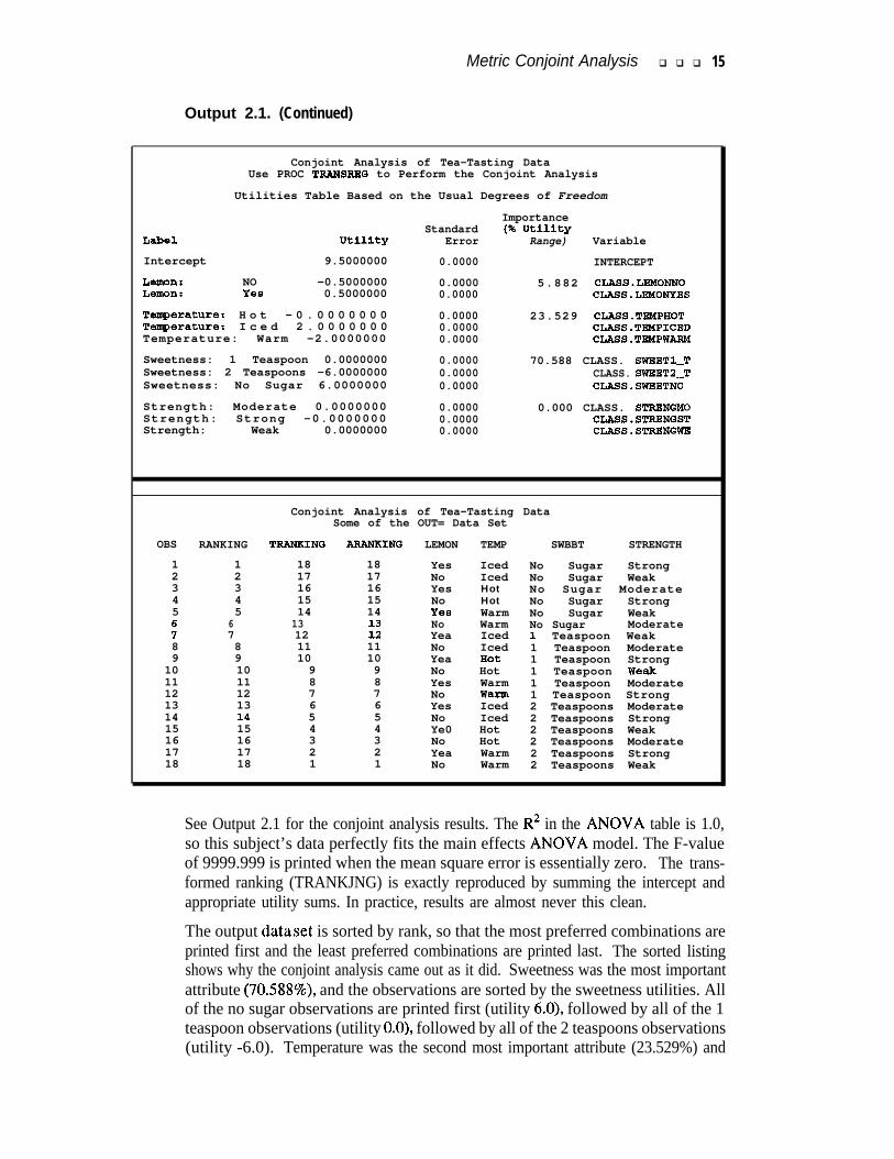
See Output 2.1 for the conjoint analysis results. The R2 in the ANOVA table is 1.0,so this subject’s data perfectly fits the main effects ANOVA model. The F-valueof 9999.999 is printed when the mean square error is essentially zero. The trans-formed ranking (TRANKJNG) is exactly reproduced by summing the intercept andappropriate utility sums. In practice, results are almost never this clean.
The output dataset is sorted by rank, so that the most preferred combinations areprinted first and the least preferred combinations are printed last. The sorted listingshows why the conjoint analysis came out as it did. Sweetness was the most importantattribute (70.588%), and the observations are sorted by the sweetness utilities. Allof the no sugar observations are printed first (utility 6.0), followed by all of the 1teaspoon observations (utility O.O), followed by all of the 2 teaspoons observations(utility -6.0). Temperature was the second most important attribute (23.529%) and
16 q q q Conjoint Analysis Examples
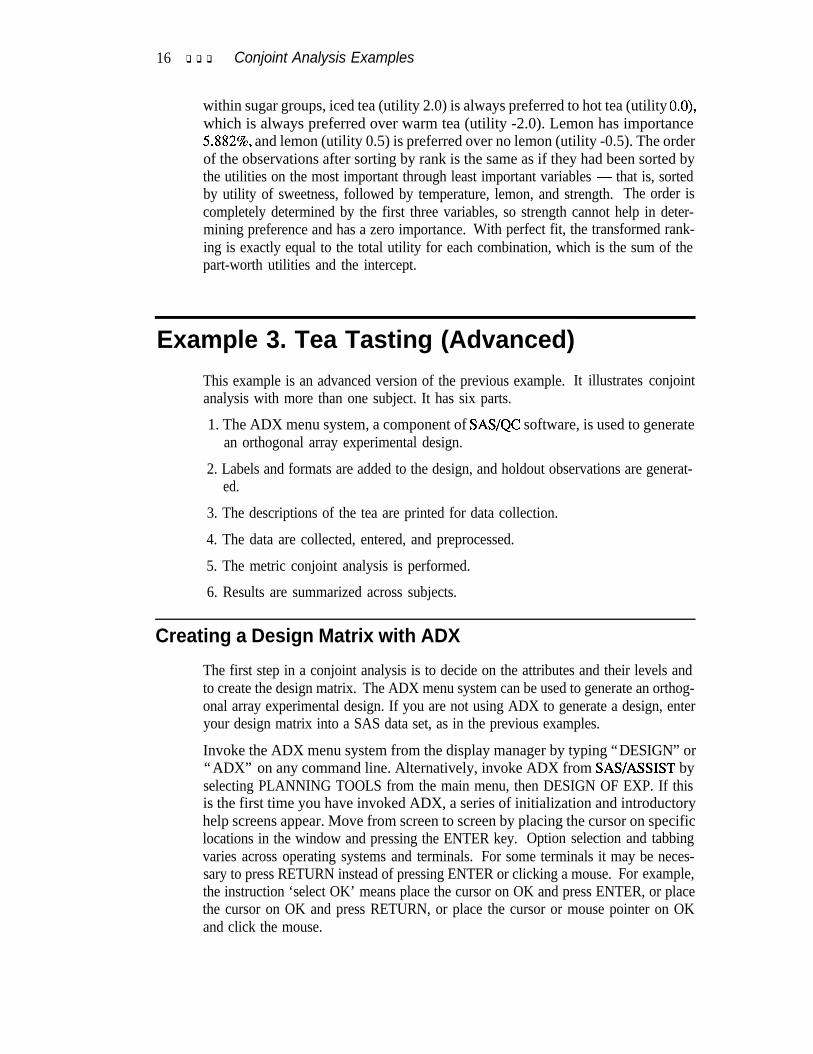
within sugar groups, iced tea (utility 2.0) is always preferred to hot tea (utility O.O),which is always preferred over warm tea (utility -2.0). Lemon has importance5.882%, and lemon (utility 0.5) is preferred over no lemon (utility -0.5). The orderof the observations after sorting by rank is the same as if they had been sorted bythe utilities on the most important through least important variables - that is, sortedby utility of sweetness, followed by temperature, lemon, and strength. The order iscompletely determined by the first three variables, so strength cannot help in deter-mining preference and has a zero importance. With perfect fit, the transformed rank-ing is exactly equal to the total utility for each combination, which is the sum of thepart-worth utilities and the intercept.
Example 3. Tea Tasting (Advanced)This example is an advanced version of the previous example. It illustrates conjointanalysis with more than one subject. It has six parts.
1. The ADX menu system, a component of SAS/QC software, is used to generatean orthogonal array experimental design.
2. Labels and formats are added to the design, and holdout observations are generat-ed.
3. The descriptions of the tea are printed for data collection.
4. The data are collected, entered, and preprocessed.
5. The metric conjoint analysis is performed.
6. Results are summarized across subjects.
Creating a Design Matrix with ADX
The first step in a conjoint analysis is to decide on the attributes and their levels andto create the design matrix. The ADX menu system can be used to generate an orthog-onal array experimental design. If you are not using ADX to generate a design, enteryour design matrix into a SAS data set, as in the previous examples.
Invoke the ADX menu system from the display manager by typing “DESIGN” or“ADX” on any command line. Alternatively, invoke ADX from SAS/ASSIST byselecting PLANNING TOOLS from the main menu, then DESIGN OF EXP. If thisis the first time you have invoked ADX, a series of initialization and introductoryhelp screens appear. Move from screen to screen by placing the cursor on specificlocations in the window and pressing the ENTER key. Option selection and tabbingvaries across operating systems and terminals. For some terminals it may be neces-sary to press RETURN instead of pressing ENTER or clicking a mouse. For example,the instruction ‘select OK’ means place the cursor on OK and press ENTER, or placethe cursor on OK and press RETURN, or place the cursor or mouse pointer on OKand click the mouse.
Creating a Design Matrix with A DX q q q 17
To create the design matrix, perform the following steps:
1. Invoke ADX.
2. If this is the first invocation of ADX, answer the initialization questions until youget to the first help screen. (Select OK. Select HIGH if you have a graphics termi-nal; otherwise, select LOW.) It is not necessary to read all of the help screens tocreate your first design. To exit the helps, select Exit Help. You will be placedin an ADX: Prompt Window and instructed to Select what you want to do:.
3. ADX automatically randomizes the design. In most experiments automatic ran-domization is desirable, and so it is the default. However, if you are workingthrough this example and wish to ensure that your results will match those present-ed here, you must turn automatic randomization off. To turn off automatic ran-domization:
a. Select NoPrompt.b. Select File.c. Select Set global parameters.d. Select No (after Automatic randomization:).e. Select OK.f. Select Help.g. Select Prompt.
You should be back in the ADX: Prompt Window, and you should again see Se-lect what you want to do:.
4. To construct the orthogonal array for this experiment, select Add a new design.If this is the first time you have invoked the ADX menu system, this will be theonly selection available.
5. The main design definition screen appears next with a prompting window request-ing a name for the design. This name will become the name of the data set holdingthe constructed design and will appear in ADX’s primary list of designs. Typethe design name, “TEA”. Select OK.
6. The design type prompt appears next. Select Orthogonal Array.
7. The next screen requests a description of the design. The descriptive label willappear in ADX’s primary list. Type “Tea-Tasting Experiment”. Select OK.
8. The next screen defines the factors of the experiment. Enter the number of levels.Type “ 1” for one 2-level factor, tab to the next field, type “3” for three 3-levelfactors, and press ENTER.
18 q q q Conjoint Analysis Examples
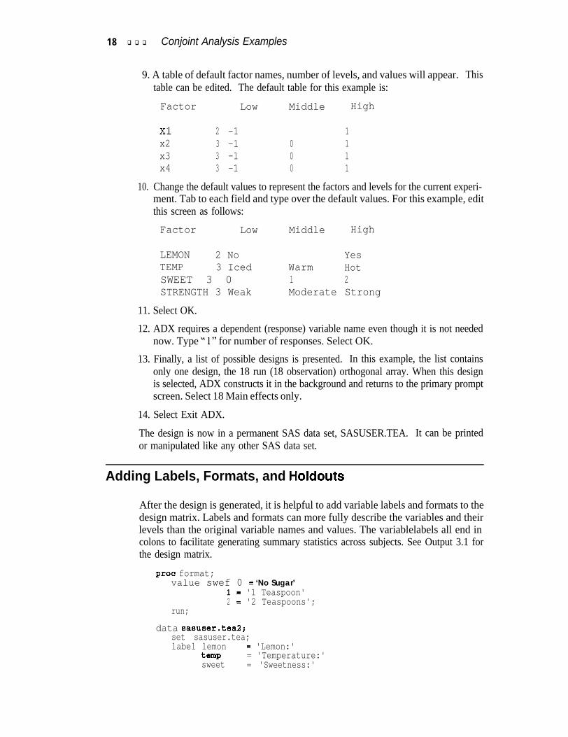
9. A table of default factor names, number of levels, and values will appear. Thistable can be edited. The default table for this example is:
Factor Low Middle High
Xl 2 -1 1x2 3 -1 0 1x3 3 -1 0 1x4 3 -1 0 1
10. Change the default values to represent the factors and levels for the current experi-ment. Tab to each field and type over the default values. For this example, editthis screen as follows:
Factor Low Middle High
LEMON 2 No YesTEMP 3 Iced Warm HotSWEET 3 0 1 2STRENGTH 3 Weak Moderate Strong
11. Select OK.
12. ADX requires a dependent (response) variable name even though it is not needednow. Type “ 1” for number of responses. Select OK.
13. Finally, a list of possible designs is presented. In this example, the list containsonly one design, the 18 run (18 observation) orthogonal array. When this designis selected, ADX constructs it in the background and returns to the primary promptscreen. Select 18 Main effects only.
14. Select Exit ADX.
The design is now in a permanent SAS data set, SASUSER.TEA. It can be printedor manipulated like any other SAS data set.
Adding Labels, Formats, and Holdouts
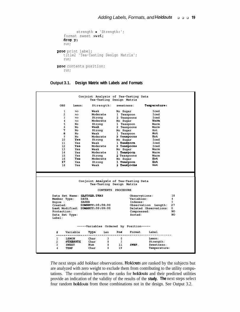
After the design is generated, it is helpful to add variable labels and formats to thedesign matrix. Labels and formats can more fully describe the variables and theirlevels than the original variable names and values. The variablelabels all end incolons to facilitate generating summary statistics across subjects. See Output 3.1 forthe design matrix.
proc format;value swef 0 = ‘No Sugar’
1 = '1 Teaspoon'2 = '2 Teaspoons';
run;
data sasuser.tea2;set sasuser.tea;label lemon = 'Lemon:'
temp = 'Temperature:'sweet = 'Sweetness:'
Adding Labels, Formats, and Holdouts q q q 19
strength = 'Strength:';format sweet swef.;drop Y;run;
proc print label;title2 'Tea-Tasting Design Matrix';run;
proc contents position;run;
Output 3.1. Design Matrix with Labels and Formats
Conjoint Analysis of Tea-Tasting DataTea-Tasting Design Matrix
OBS Lemon: Strength: sweetness: Temerature:
1 NO Weak No Sugar Iced2 NO Moderate 1 Teaspoon Iced3 NO Strong 2 Teaspoons Iced4 NO Moderate No Sugar Warm5 No Strong 1 Teaspoon Warm6 No Weak 2 Teaspoons Warm7 No Strong No Sugar Hot8 No Weak 1 Teaspoon Hot9 No Moderate 2 TeaagOOna Hot
10 Yea Strong No Sugar Iced11 Yes Weak 1 Teaspoon Iced12 Yes Moderate 2 TeaSgOOnS Iced13 Yes Weak No Sugar Warm14 Yes Moderate 1 Teaspoon Warm15 Yes Strong 2 Teaspoons Warm16 Ye9 Moderate No Sugar Hot11 Yea Strong 1 TeaSgOOn Hot18 Yea Weak 2 Tea0pOOns Hot
Conjoint Analysis of Tea-Tasting DataTea-Tasting Design Matrix
CONTENTS PROCEDURE
Data Set Name: SASUSER.TEAPMember Type: DATAEngine : SASEBCreated: DDMMMYY:OO:00:00Last Modified: DDMMMYY:00:00:00Protection:Data Set Type:Label:
Observations: 18Variables: 4Indexes: 0Observation Length: 27Deleted Observations: 0Compressed: NOSorted: NO
-----Variables Ordered by Position-----
# Variable 'Ww Len POS Format Label____________________--------------------------------- - - - - - - - -1 LEMON Char 3 0 Lemon:2 STRBNQTH Char 8 3 Strength:3 SWEET Num 8 11 SWBF . Sweetness:4 TEMP Char 8 19 Temperature:
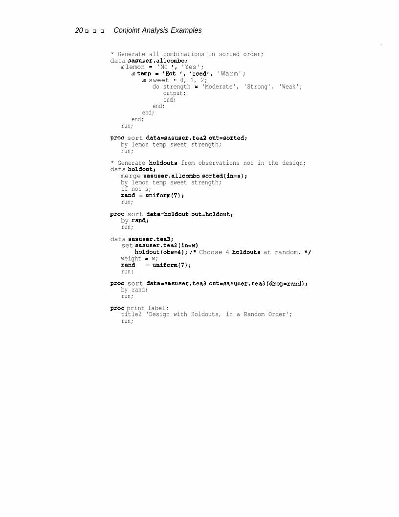
The next steps add holdout observations. Holdouts are ranked by the subjects butare analyzed with zero weight to exclude them from contributing to the utility compu-tations. The correlation between the ranks for holdouts and their predicted utilitiesprovide an indication of the validity of the results of the study. The next steps selectfour random holdouts from those combinations not in the design. See Output 3.2.
20 q q q Conjoint Analysis Examples
* Generate all combinations in sorted order;data sasuser.allcombo;
a0 lemon = ‘NO I, 'Yes';a0 ternp = 'Hot II 'Icedrp 'Warm';
a0 sweet = 0, 1, 2;do strength = 'Moderate', 'Strong', 'Weak';
output:end;
end;end;
end;run;
proc sort datamsasuser.tea2 outksorted;by lemon temp sweet strength;run;
* Generate holdouts from observations not in the design;data holdout;
merge sasuser.allcombo sorted(in=s);by lemon temp sweet strength;if not s;rand = uniform(7);run;
proc sort data=holdout oukholdout;by rand;run;
data sasuser.tea3;set sasuser.tea2(in=w)
holdout(obs4); /* Choose 4 holdouts at random. */weight = w;rand = uniform(7);run:
proc sort data=sasuser.tea3 out=sasuser.tea3(drop=rand);by rand;run;
proc print label;title2 'Design with Holdouts, in a Random Order';run;
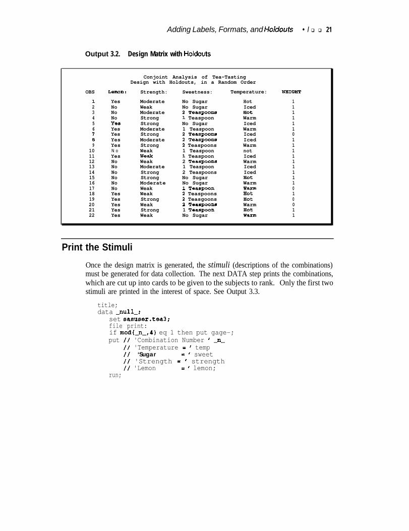
Adding Labels, Formats, and Holdouts •I q q 21
Output 3.2. Design Matrix with Holdouts
Conjoint Analysis of Tea-TastingDesign with Holdouts, in a Random Order
OBS Lemn: Strength: Sweetness: Temperature: WBIQHT
1 Yes Moderate No Sugar Hot 12 No Weak No Sugar Iced 13 No Moderate 2 TeaSgOOns Hot 14 No Strong 1 Teaspoon Warm 15 Y0S Strong No Sugar Iced 16 Yes Moderate 1 Teaspoon Warm 17 Yes Strong 2 TeaSgOOnS Iced 08 Yes Moderate 2 TeaSgOOnS Iced 19 Yes Strong 2 Teaspoons Warm 1
10 N o Weak 1 Teaspoon not 111 Yes Weak 1 Teaspoon Iced 112 No Weak 2 TeaSpOOns Warm 113 No Moderate 1 Teaspoon Iced 114 No Strong 2 Teaspoons Iced 115 No Strong No Sugar Hot 116 No Moderate No Sugar Warm 117 No Weak 1 TeaSgOOn wal-ltl 018 Yes Weak 2 Teaspoons Hot 119 Yes Strong 2 Teasgoons Hot 020 Yes Weak 2 TeaspOOnS Warm 021 Yes Strong 1 TeaSgOOn l-lot 122 Yes Weak No Sugar WWL-lll 1
Print the Stimuli
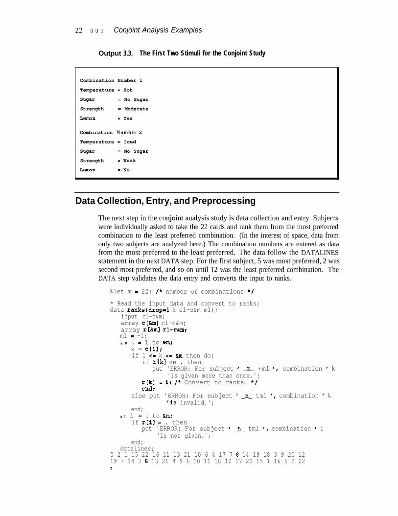
Once the design matrix is generated, the stimuli (descriptions of the combinations)must be generated for data collection. The next DATA step prints the combinations,which are cut up into cards to be given to the subjects to rank. Only the first twostimuli are printed in the interest of space. See Output 3.3.
title;data -null-;
set sasuser.tea3;file print:if mod(-n-,4) eq 1 then put gage-;put // 'Combination Number ' -n-
// 'Temperature = ' temp// ‘Sugar = ' sweet// 'Strength = ' strength// 'Lemon = f lemon;
run;
22 q q q Conjoint Analysis Examples
Output 3.3. The First Two Stimuli for the Conjoint Study
Combination Number 1
Temperature = Hot
Sugar = No Sugar
Strength = Moderate
Lemon = Yes
Combination Number 2
Temperature = Iced
Sugar = No Sugar
Strength = Weak
Lemon = No
Data Collection, Entry, and Preprocessing
The next step in the conjoint analysis study is data collection and entry. Subjectswere individually asked to take the 22 cards and rank them from the most preferredcombination to the least preferred combination. (In the interest of space, data fromonly two subjects are analyzed here.) The combination numbers are entered as datafrom the most preferred to the least preferred. The data follow the DATALINESstatement in the next DATA step. For the first subject, 5 was most preferred, 2 wassecond most preferred, and so on until 12 was the least preferred combination. TheDATA step validates the data entry and converts the input to ranks.
%let m = 22; /* number of combinations */
* Read the input data and convert to ranks;data ranks(drop=i k cl-c&m ml);
input cl-c&m;array c[&ml cl-c&m;array r[&ml rl-r&m;ml = -1;a 0 i = 1 to &m;
k = c[i];if 1 <= k <= &m then do;
if r[kI ne . thenput 'ERROR: For subject ' -n- +ml ', combination ' k
'is given more than once.';r [kl = i; /* Convert to ranks. */end;
else put 'ERROR: For subject ' -n- tml ', combination ' k'is invalid.';
end;a 0 i = 1 to &m;
if r[i] = . thenput 'ERROR: For subject ' -n- tml ', combination ' i
'is not given.';end;
datalines;5 2 1 15 22 16 11 13 21 10 6 4 17 7 8 14 19 18 3 9 20 1219 7 14 3 8 13 21 4 9 6 10 11 18 12 17 20 15 1 16 5 2 22;
Data Collection, Entry, and Preprocessing 0 0 0 23
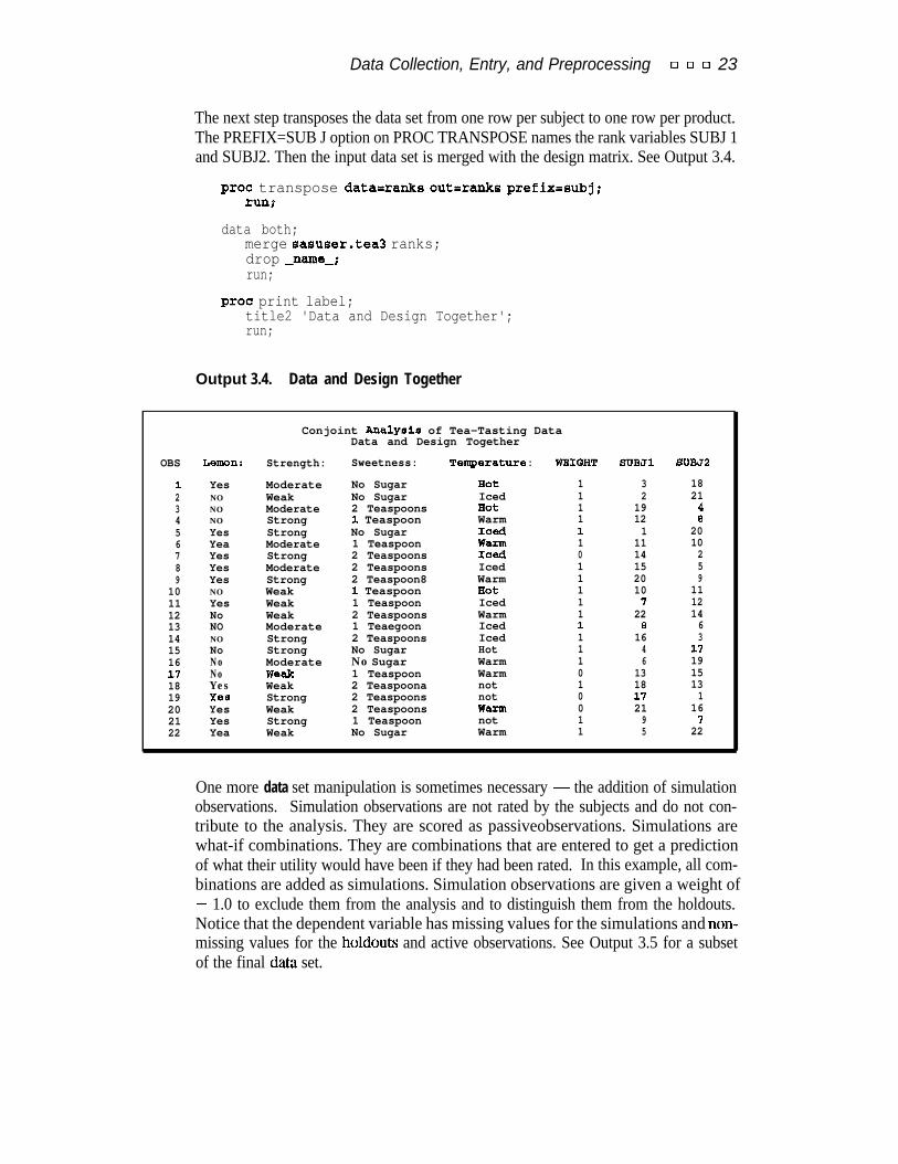
The next step transposes the data set from one row per subject to one row per product.The PREFIX=SUB J option on PROC TRANSPOSE names the rank variables SUBJ 1and SUBJ2. Then the input data set is merged with the design matrix. See Output 3.4.
proc transpose data=ranks out=ranks prefix=subj;run9
data both;merge sasuser.tea3 ranks;drop -name-;run;
proc print label;title2 'Data and Design Together';run;
Output 3.4. Data and Design Together
Conjoint Analyeie of Tea-Tasting DataData and Design Together
OBS Lemm: Strength: Sweetness: Temperature : WBIQHT SUBJl SUBJ2
1 Yes Moderate No Sugar Hot 1 3 182 NO Weak No Sugar Iced 1 2 213 NO Moderate 2 Teaspoons Hot 1 19 44 NO Strong 1 Teaspoon Warm 1 12 85 Yes Strong No Sugar Iced 1 1 206 Yea Moderate 1 Teaspoon Warm 1 11 107 Yes Strong 2 Teaspoons Iced 0 14 28 Yes Moderate 2 Teaspoons Iced 1 15 59 Yes Strong 2 Teaspoon8 Warm 1 20 9
10 NO Weak 1 Teaspoon Hot 1 10 1111 Yes Weak 1 Teaspoon Iced 1 7 1212 No Weak 2 Teaspoons Warm 1 22 1413 NO Moderate 1 Teaegoon Iced 1 8 614 NO Strong 2 Teaspoons Iced 1 16 315 No Strong No Sugar Hot 1 4 1116 No Moderate No Sugar Warm 1 6 1911 No Weak 1 Teaspoon Warm 0 13 1518 Yes Weak 2 Teaspoona not 1 18 1319 Yes Strong 2 Teaspoons not 0 17 120 Yes Weak 2 Teaspoons Warm 0 21 1621 Yes Strong 1 Teaspoon not 1 9 722 Yea Weak No Sugar Warm 1 5 22
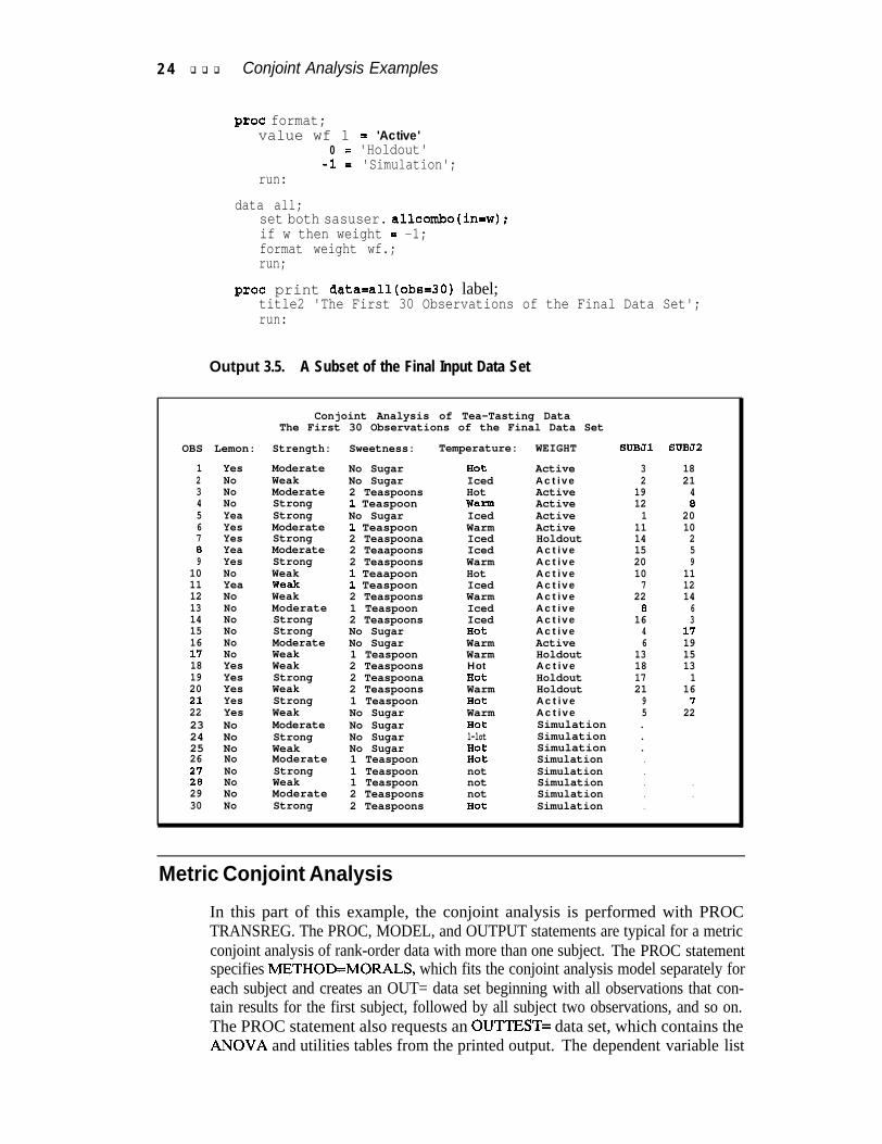
One more data set manipulation is sometimes necessary - the addition of simulationobservations. Simulation observations are not rated by the subjects and do not con-tribute to the analysis. They are scored as passiveobservations. Simulations arewhat-if combinations. They are combinations that are entered to get a predictionof what their utility would have been if they had been rated. In this example, all com-binations are added as simulations. Simulation observations are given a weight of- 1.0 to exclude them from the analysis and to distinguish them from the holdouts.Notice that the dependent variable has missing values for the simulations and non-missing values for the holdouts and active observations. See Output 3.5 for a subsetof the final data set.
2 4 q q q Conjoint Analysis Examples
proc format;value wf 1 = 'Active'
0 = 'Holdout'-1 = 'Simulation';
run:
data all;set both sasuser. allcombo(in=w);if w then weight = -1;format weight wf.;run;
proc print data=all(obs=30) label;title2 'The First 30 Observations of the Final Data Set';run:
Output 3.5. A Subset of the Final Input Data Set
Conjoint Analysis of Tea-Tasting DataThe First 30 Observations of the Final Data Set
OBS Lemon: Strength: Sweetness: Temperature: WEIGHT SUBJl SVBJZ
1 Yes Moderate No Sugar Hot Active 3 182 No Weak No Sugar Iced Active 2 213 No Moderate 2 Teaspoons Hot Active 19 44 No Strong 1 Teaspoon Warm Active 12 85 Yea Strong No Sugar Iced Active 1 206 Yes Moderate 1 Teaspoon Warm Active 11 107 Yes Strong 2 Teaspoona Iced Holdout 14 28 Yea Moderate 2 Teaapoons Iced Active 15 59 Yes Strong 2 Teaspoons Warm Active 20 9
10 No Weak 1 Teaapoon Hot Active 10 1111 Yea Weak 1 Teaspoon Iced Active 7 1212 No Weak 2 Teaspoons Warm Active 22 1413 No Moderate 1 Teaspoon Iced Active 8 614 No Strong 2 Teaspoons Iced Active 16 315 No Strong No Sugar Hot Active 4 1716 No Moderate No Sugar Warm Active 6 1917 No Weak 1 Teaspoon Warm Holdout 13 1518 Yes Weak 2 Teaspoons Hot Active 18 1319 Yes Strong 2 Teaspoona Hot Holdout 17 120 Yes Weak 2 Teaspoons Warm Holdout 21 1621 Yes Strong 1 Teaspoon Hot Active 9 722 Yes Weak No Sugar Warm Active 5 2223 No Moderate No Sugar Hot Simulation .24 No Strong No Sugar l-lot Simulation .25 No Weak No Sugar Hot Simulation .26 No Moderate 1 Teaspoon Hot Simulation .21 No Strong 1 Teaspoon not Simulation .28 No Weak 1 Teaspoon not Simulation . .29 No Moderate 2 Teaspoons not Simulation . .30 No Strong 2 Teaspoons Hot Simulation .
Metric Conjoint Analysis
In this part of this example, the conjoint analysis is performed with PROCTRANSREG. The PROC, MODEL, and OUTPUT statements are typical for a metricconjoint analysis of rank-order data with more than one subject. The PROC statementspecifies MEWHOD=MORALS, which fits the conjoint analysis model separately foreach subject and creates an OUT= data set beginning with all observations that con-tain results for the first subject, followed by all subject two observations, and so on.The PROC statement also requests an OUTTEST= data set, which contains theANOVA and utilities tables from the printed output. The dependent variable list
Metric Conjoint Analysis 0 0 0 25
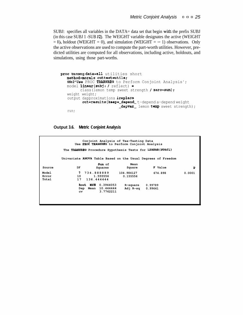
SUBJ: specifies all variables in the DATA= data set that begin with the prefix SUBJ(in this case SUBJ 1 -SUB 52). The WEIGHT variable designates the active (WEIGHT= l), holdout (WEIGHT = 0), and simulation (WEIGHT = - 1) observations. Onlythe active observations are used to compute the part-worth utilities. However, pre-dicted utilities are computed for all observations, including active, holdouts, andsimulations, using those part-worths.
proc transreg data=all utilities shortmethod=morals outtest-utils;title2 'Use PROC TRANSREG to Perform Conjoint Analysis';model linear(subj: / reflect) =
class(lemon temp sweet strength / zeroesurn);weight weight;output dapproximations ireplace
out=results(keep=-depend- t-depend a-depend weight-depvar- lemon temp sweet strength);
run;
Output 3.6. Metric Conjoint Analysis
Conjoint Analysis of Tea-Tasting DataUee PRCC TRANSREQ to Perform Conjoint Analysis
The TRANSREQ Procedure Hypothesis Tests for LINEAR(SUBJ1)
Univariate ANOVA Table Based on the Usual Degrees of Freedom
Source
ModelErrorTotal
sum of MeanDF Squares Square F Value PI 7 3 4 . 8 8 8 8 8 9 104.984127 674.898 0.000110 1.555556 0.15555617 136.444444
Root MSE 0.3944053 R-square 0.99789Dep Mean 10.444444 Adj R-sq 0.99641cv 3.7762211
2 6 q q q Conjoint Analysis Examples
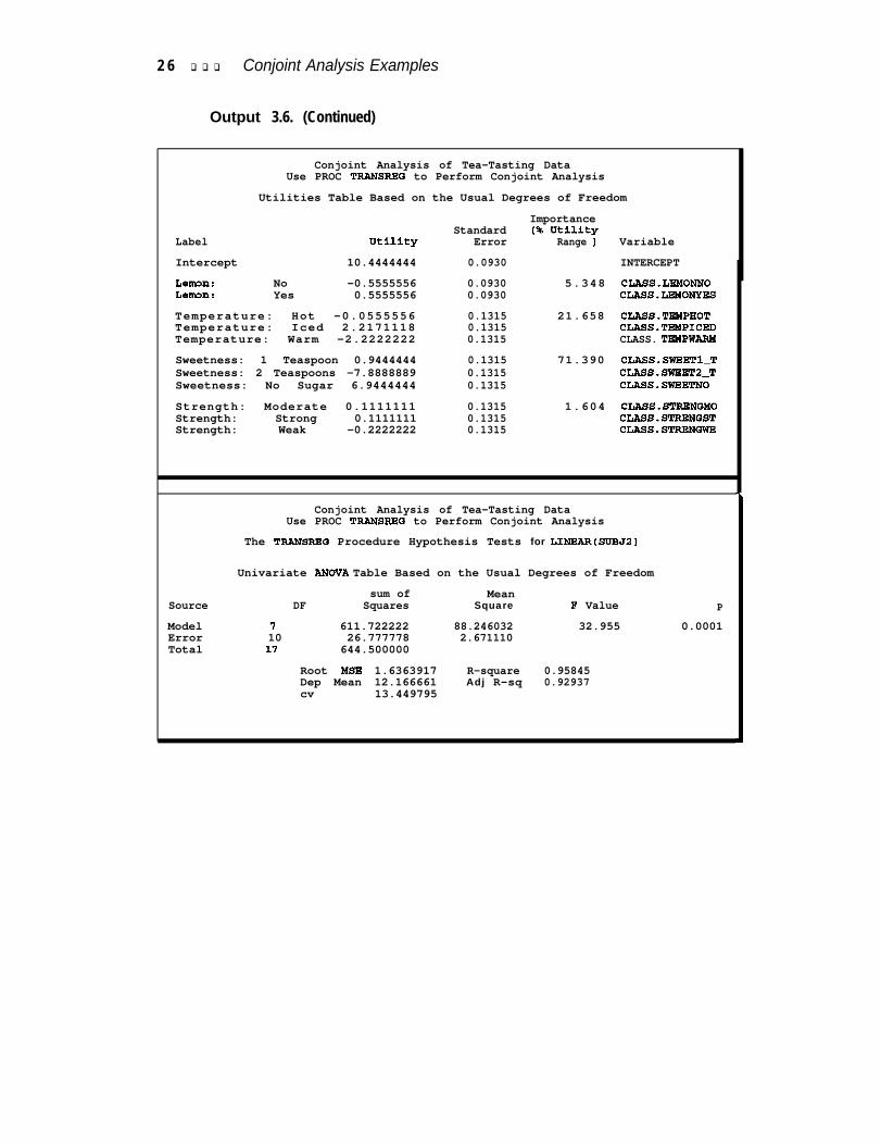
Output 3.6. (Continued)
Conjoint Analysis of Tea-Tasting DataUse PROC TRANSREQ to Perform Conjoint Analysis
Utilities Table Based on the Usual Degrees of Freedom
ImportanceStandard (% Utility
Label Utility Error Range ) Variable
Intercept 10.4444444 0.0930 INTERCEPT
Lemon: No -0.5555556 0.0930 5.348 cL?iSs.LxMoNNoLemon: Yes 0.5555556 0.0930 CL&SS.LBMONYES
Temperature: Hot -0.0555556 0.1315 21.658 CLASS.TRMPHOTTemperature: Iced 2.2171118 0.1315 CLASS.TBMPICEDTemperature: Warm -2.2222222 0.1315 CLASS. TBMPWARM
Sweetness: 1 Teaspoon 0.9444444 0.1315 71.390 CLASS.SWBETl-TSweetness: 2 Teaspoons -7.8888889 0.1315 C!LASS.SWBET2-TSweetness: No Sugar 6.9444444 0.1315 CLASS.SWBEETNO
Strength: Moderate 0.1111111 0.1315 1.604 CLASS.STRENQMOStrength: Strong 0.1111111 0.1315 CLASS.STRBNQSTStrength: Weak -0.2222222 0.1315 CLASS.STRENGWE
Conjoint Analysis of Tea-Tasting DataUse PROC TRANSRBQ to Perform Conjoint Analysis
The TRANSREQ Procedure Hypothesis Tests for LINSAR(SUBJ2)
Univariate ANOVA Table Based on the Usual Degrees of Freedomsum of Mean
Source DF Squares Square F Value P
Model I 611.722222 88.246032 32.955 0.0001Error 10 26.777778 2.671110Total 11 644.500000
Root MSE 1.6363917 R-square 0.95845Dep Mean 12.166661 Adj R-sq 0.92937cv 13.449795
Metric Conjoint Analysis q q q 27
Output 3.6. (Continued)
Conjoint Analysis of Tea-Tasting DataUse PRCC TRANSRRG to Perform Conjoint Analysis
Utilities Table Based on the Usual Degrees of Freedom
ImportanceStandard (96 Utility
Lab81 Utility Error Range) Variable
Intercept 12.1666667 0.3857 INTERCEPT
Lemon: No 0.7222222 0.3857 7.008 CLASS.LRbfONNOLemon: Yes -0.7222222 0.3857 CLASS.LRMOmES
Temperature: Hot 0.5000000 0.5455 12.129 CLASS.TRMPHOTTemperature: Iced 1.0000000 0.5455 CL?iSS.TRMPICEDTemperature: Warm -1.5000000 0.5455 C!LASS.TRMPWAPM
Sweetness: 1 Teaspoon 3.1666667 0.5455 55.795 CL?iSS.SWRRTl-TSweetness: 2 Teaspoons 4.1666667 0.5455 CL?hSS.SWEEET2-TSweetness: No Sugar -7.3333333 0.5455 CLASS.SWRETNO
Strength: Moderate 1.6333333 0.5455 25.067 CLASS.STRENGMOStrength: Strong 1.5000000 0.5455 CLASS. STRRNGSTStrength: Weak -3.3333333 0.5455 CLASS.STRRNGWE
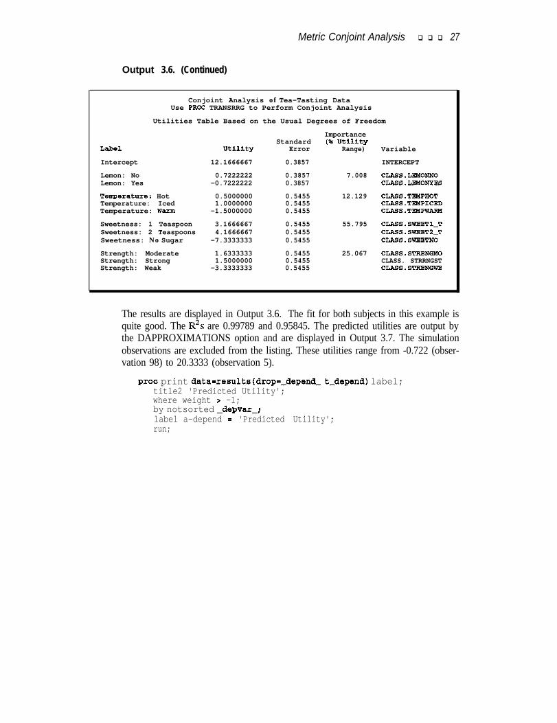
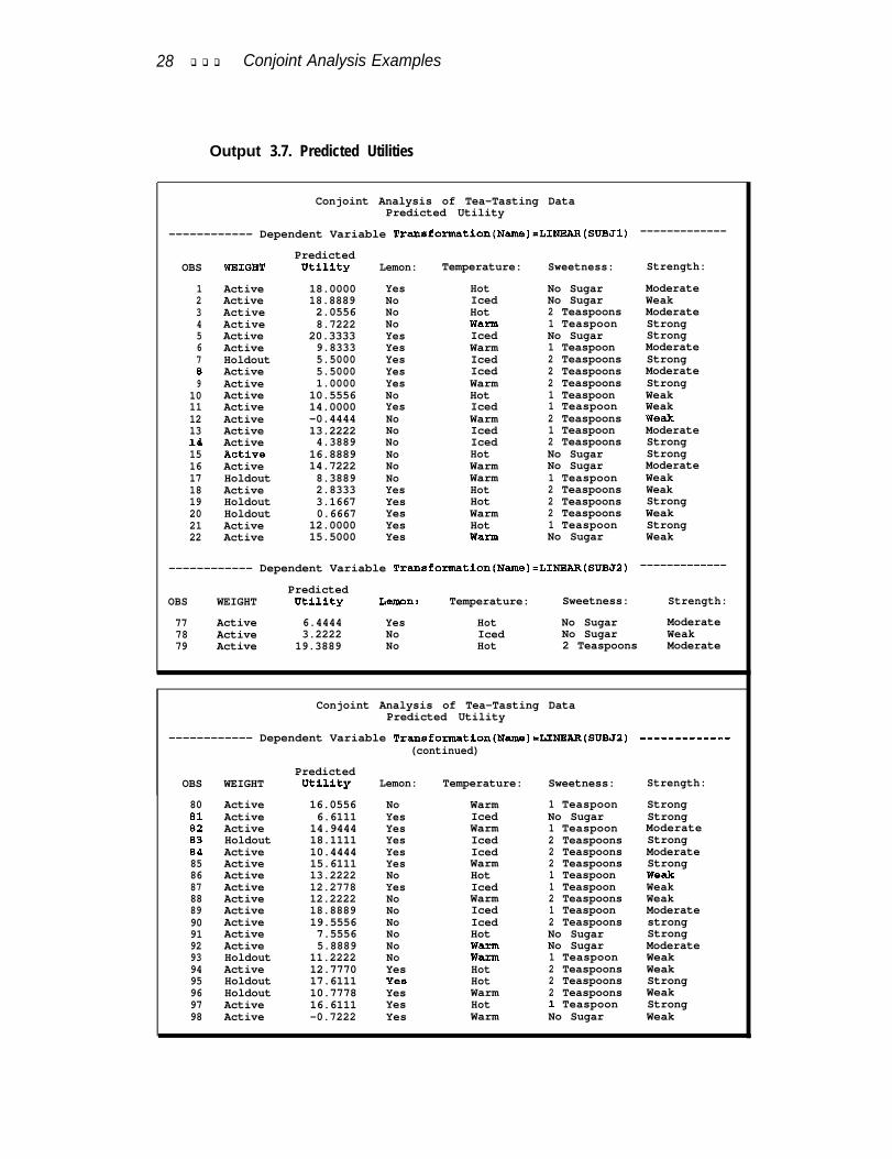
The results are displayed in Output 3.6. The fit for both subjects in this example isquite good. The R2s are 0.99789 and 0.95845. The predicted utilities are output bythe DAPPROXIMATIONS option and are displayed in Output 3.7. The simulationobservations are excluded from the listing. These utilities range from -0.722 (obser-vation 98) to 20.3333 (observation 5).
proc print data=results(drop=-depend-t-depend) label;title2 'Predicted Utility';where weight > -1;by notsorted -depvar-;label a-depend = 'Predicted Utility';run;
28 q q q Conjoint Analysis Examples
Output 3.7. Predicted Utilities
Conjoint Analysis of Tea-Tasting DataPredicted Utility
------------ Dependent Variable Transfo?matlon(Name)=LINBAR(SUBJ1) -------------
OBS WEIGHT
123456789
1011121314151617
Active 18.0000 Yes Hot No Sugar ModerateActive 18.8889 No Iced No Sugar WeakActive 2.0556 No Hot 2 Teaspoons ModerateActive 8.7222 No Warm 1 Teaspoon StrongActive 20.3333 Yes Iced No Sugar StrongActive 9.8333 Yes Warm 1 Teaspoon ModerateHoldout 5.5000 Yes Iced 2 Teaspoons StrongActive 5.5000 Yes Iced 2 Teaspoons ModerateActive 1.0000 Yes Warm 2 Teaspoons StrongActive 10.5556 No Hot 1 Teaspoon WeakActive 14.0000 Yes Iced 1 Teaspoon WeakActive -0.4444 No Warm 2 Teaspoons WeakActive 13.2222 No Iced 1 Teaspoon ModerateActive 4.3889 No Iced 2 Teaspoons StrongActfve 16.8889 No Hot No Sugar StrongActive 14.7222 No Warm No Sugar ModerateHoldout 8.3889 No Warm 1 Teaspoon WeakActive 2.8333 Yes Hot 2 Teaspoons WeakHoldout 3.1667 Yes Hot 2 Teaspoons StrongHoldout 0.6667 Yes Warm 2 Teaspoons WeakActive 12.0000 Yes Hot 1 Teaspoon StrongActive 15.5000 Yes Warm No Sugar Weak
1819202122
PredictedUtility Lemon: Temperature: Sweetness: Strength:
------------ Dependent Variable Transformation(Name)=LINEAR(SUBJ2) -------------
PredictedOBS WEIGHT Utility Lemx: Temperature: Sweetness: Strength:
77 Active 6.4444 Yes Hot No Sugar Moderate78 Active 3.2222 No Iced No Sugar Weak79 Active 19.3889 No Hot 2 Teaspoons Moderate
Conjoint Analysis of Tea-Tasting DataPredicted Utility
------------ Dependent Variable Transformatlon(Name)=LINBAR(SUBJ2)(continued)
PredictedOBS WEIGHT Utility Lemon: Temperature: Sweetness:
80 Active 16.0556 No Warm 1 Teaspoon Strong81 Active 6.6111 Yes Iced No Sugar Strong82 Active 14.9444 Yes Warm 1 Teaspoon Moderate83 Holdout 18.1111 Yes Iced 2 Teaspoons Strong84 Active 10.4444 Yes Iced 2 Teaspoons Moderate85 Active 15.6111 Yes Warm 2 Teaspoons Strong86 Active 13.2222 No Hot 1 Teaspoon Weak87 Active 12.2778 Yes Iced 1 Teaspoon Weak88 Active 12.2222 No Warm 2 Teaspoons Weak89 Active 18.8889 No Iced 1 Teaspoon Moderate90 Active 19.5556 No Iced 2 Teaspoons strong91 Active 7.5556 No Hot No Sugar Strong92 Active 5.8889 No Warm No Sugar Moderate93 Holdout 11.2222 No Warm 1 Teaspoon Weak94 Active 12.7770 Yes Hot 2 Teaspoons Weak95 Holdout 17.6111 Yea Hot 2 Teaspoons Strong96 Holdout 10.7778 Yes Warm 2 Teaspoons Weak97 Active 16.6111 Yes Hot 1 Teaspoon Strong98 Active -0.7222 Yes Warm No Sugar Weak
-------------
Strength:
Metric Conjoint Analysis q q q 29
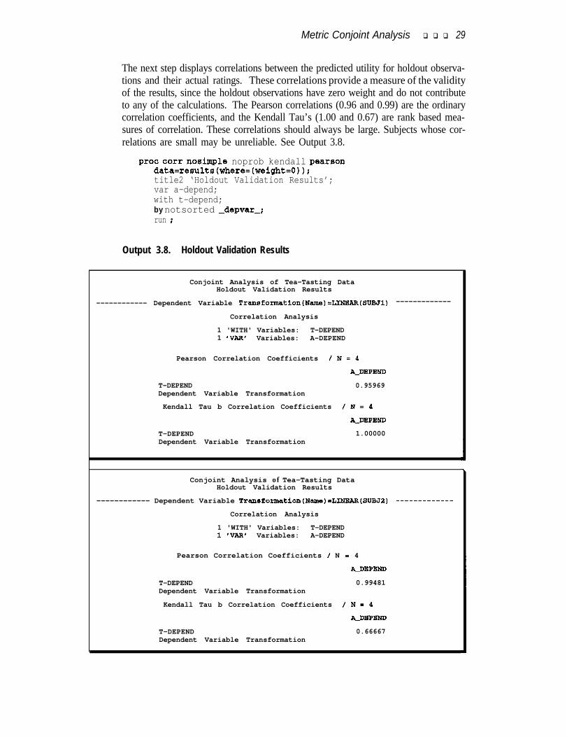
The next step displays correlations between the predicted utility for holdout observa-tions and their actual ratings. These correlations provide a measure of the validityof the results, since the holdout observations have zero weight and do not contributeto any of the calculations. The Pearson correlations (0.96 and 0.99) are the ordinarycorrelation coefficients, and the Kendall Tau’s (1.00 and 0.67) are rank based mea-sures of correlation. These correlations should always be large. Subjects whose cor-relations are small may be unreliable. See Output 3.8.
proc corr nosimple noprob kendall pearsondata=results(where=(weight=O));title2 ‘Holdout Validation Results’;var a-depend;with t-depend;by notsorted -depvar-;run ;
Output 3.8. Holdout Validation Results
Conjoint Analysis of Tea-Tasting DataHoldout Validation Results
------------ Dependent Variable Transformatlon(Name)=LINRAR(SUBJl) -------------
Correlation Analysis
1 'WITH' Variables: T-DEPEND1 'VAR' Variables: A-DEPEND
Pearson Correlation Coefficients /N=4
A-DRPEND
T-DEPEND 0.95969Dependent Variable Transformation
Kendall Tau b Correlation Coefficients /N=4
A-DEPEND
T-DEPEND 1.00000Dependent Variable Transformation
Conjoint Analysis of Tea-Tasting DataHoldout Validation Results
------------ Dependent Variable Transformatlon(Name)=LINRAR(SUBJ2) ______-______
Correlation Analysis
1 'WITH' Variables: T-DEPEND1'VAR' Variables: A-DEPEND
Pearson Correlation Coefficients / N = 4
A-DRPEND
T-DEPEND 0.99481Dependent Variable Transformation
Kendall Tau b Correlation Coefficients /N=4
A-DRPEND
T-DEPEND 0.66667Dependent Variable Transformation
3 0 q q q Conjoint Analysis Examples
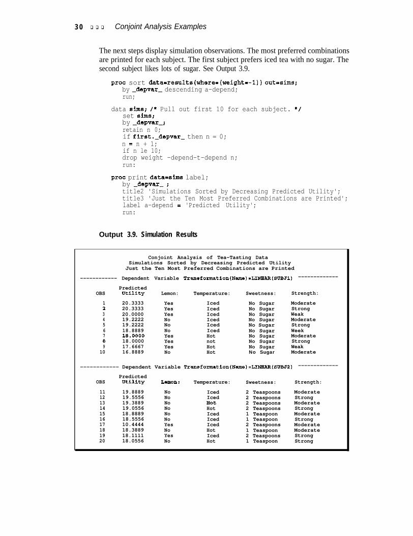
The next steps display simulation observations. The most preferred combinationsare printed for each subject. The first subject prefers iced tea with no sugar. Thesecond subject likes lots of sugar. See Output 3.9.
proc sort data=results(where=(weight=-1)) outxsims;by -depvar- descending a-depend;run;
data Sims; /* Pull out first 10 for each subject. */set Sims;by -depvar-;retain n 0;if first.-depvar- then n = 0;n = n + 1;if n le 10;drop weight -depend-t-depend n;run:
proc print data=sims label;by -depvar- ;title2 'Simulations Sorted by Decreasing Predicted Utility';title3 'Just the Ten Most Preferred Combinations are Printed';label a-depend = 'Predicted Utility';run:
Output 3.9. Simulation Results
Conjoint Analysis of Tea-Tasting DataSimulations Sorted by Decreasing Predicted Utility
Just the Ten Most Preferred Combinations are Printed
------------ Dependent Variable Transformatlon(Name)=LINBAR(SUBJl) -------------
PredictedOBS Utility Lemon: Temperature: Sweetness: Strength:
1 20.3333 Yes Iced No Sugar Moderate2 20.3333 Yes Iced No Sugar Strong3 20.0000 Yes Iced No Sugar Weak4 19.2222 No Iced No Sugar Moderate5 19.2222 No Iced No Sugar Strong6 18.8889 No Iced No Sugar Week7 1a.0000 Yes Hot No Sugar Moderate8 18.0000 Yes not No Sugar Strong9 17.6667 Yes Hot No Sugar Weak
10 16.8889 No Hot No Sugar Moderate
------------ Dependent Variable Transformation(Name)=LINEAH(SUBJ2) -------------
PredictedOBS Utility Lermn: Temperature: Sweetness: Strength:
11 19.8889 No Iced 2 Teaspoons Moderate12 19.5556 No Iced 2 Teaspoons Strong13 19.3889 No Hot 2 Teaspoons Moderate14 19.0556 No Hot 2 Teaspoons Strong15 18.8889 No Iced 1 Teaspoon Moderate16 18.5556 No Iced 1 Teaspoon Strong17 10.4444 Yes Iced 2 Teaspoons Moderate18 18.3889 No Hot 1 Teaspoon Moderate19 18.1111 Yes Iced 2 Teaspoons Strong20 18.0556 No Hot 1 Teaspoon Strong
Summarizing Results Across Subjects q q q 31
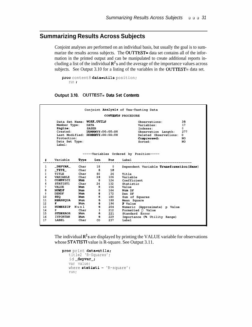
Summarizing Results Across Subjects
Conjoint analyses are performed on an individual basis, but usually the goal is to sum-marize the results across subjects. The OUTTEST= data set contains all of the infor-mation in the printed output and can be manipulated to create additional reports in-cluding a list of the individual R2s and the average of the importance values acrosssubjects. See Output 3.10 for a listing of the variables in the OUTTEST= data set.
proc content8 data=utils position;run r’
Output 3.10. OUTTEST= Data Set Contents
Conjoint Analysis of Tea-Tasting Data
CONTBNTS PROCEDURE
Data Set Name: WORK.UTILSMember Type: DATAEngine : SASEBCreated: DDMMMYY:00:00:00Last Modified: DDMMMYY:OO:OO:OOProtection:Data Set Type:Label:
Observations: 38Variables: 17Indexes: 0Observation Length: 277Deleted Observations: 0Corngreased: NOSorted: NO
-----Variables Ordered by Position-----
# Variable Tme Len POS Label-------------------------------------------------------------------------------1 -DEPVAR- Char 18 0 Dependent Variable Transformation(Name)2 -TYPE- Char a 183 TITLE Char 80 26 Title4 VARIABLE Char 18 106 Variable5 COEFFICI Nun 8 124 Coefficient6 STATIST1 Char 24 132 Statistic7 VALUE Nun e 156 Valuee NUNDF Num e 164 Nurn DF9 DENDF NUlTl 8 172 Den DF
10 SSQ NUm 8 180 Sum of Squares11 MEANSQUA Num 8 188 Mean Square12 F NUm 8 196 F Value13 NUMERICP N u n l 8 204 Numeric (Approximate) p Value14 P Char 9 212 Formatted p Value15 STDERROR Num e 221 Standard Error16 IYPORTAN Num e 229 Importance (% Utility Range)17 LABEL Char CO 237 Label
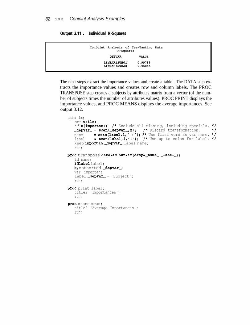
The individual R2s are displayed by printing the VALUE variable for observationswhose STATISTI value is R-square. See Output 3.11.
proc print data=utils;title2 ‘R-Squares’;id -depvar-;var value;where statieti = ‘R-square’:run;
32 q q q Conjoint Analysis Examples
Output 3.11 m Individual R-Squares
Conjoint Analysis of Tea-Tasting DataR-Squares
-DEPVAR- VALUE
LINEAR(SUBJ1) 0.99789LINEAR(SUBJ2) 0.95845
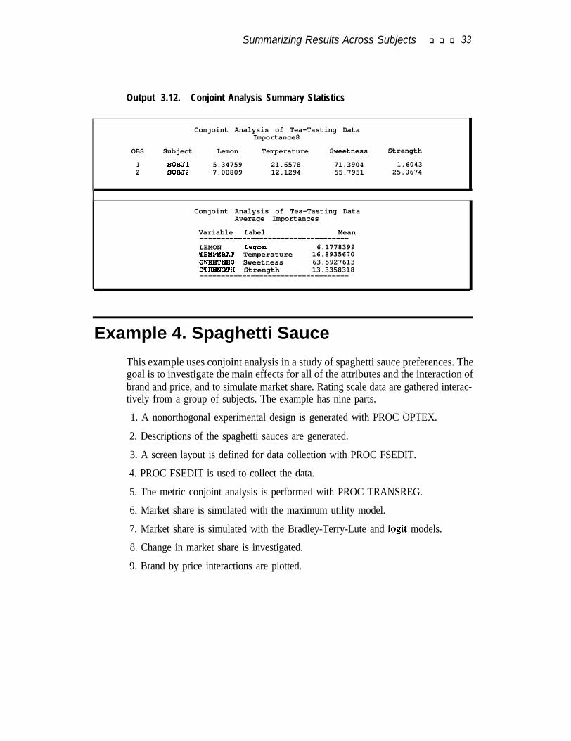
The next steps extract the importance values and create a table. The DATA step ex-tracts the importance values and creates row and column labels. The PROCTRANSPOSE step creates a subjects by attributes matrix from a vector (of the num-ber of subjects times the number of attributes values). PROC PRINT displays theimportance values, and PROC MEANS displays the average importances. Seeoutput 3.12.
data im;set utils;if n(importan); /* Exclude all missing, including specials. */-depvar- = scan(-depvar-,2); /* Discard transformation. */name = scan(label,l,' : I); I* Use first word as var name. */label = scan(label,l,':'); /* Use up to colon for label. */keep importan -depvar- label name;run;
proc transpose data=im out=im(drop=~name~~label~);id name;idlabel label;by notsorted -depvar-;var importan;label -depvar- = 'Subject';run;
proc print label;title2 'Importances';run;
proc means mean;title2 'Average Importances';run;
Summarizing Results Across Subjects q q q 33
Output 3.12. Conjoint Analysis Summary Statistics
Conjoint Analysis of Tea-Tasting DataImportance8
OBS Subject Lemon Temperature Sweetness Strength
1 SUBJl 5.34759 21.6578 71.3904 1.60432 SIJBJS 7.00809 12.1294 55.7951 25.0674
Conjoint Analysis of Tea-Tasting DataAverage Importances
Variable Label Mean-----------------------------------LEMON Leman 6.1778399TEMPERAT Temperature 16.8935670SWBETNES Sweetness 63.5927613STRENGTH Strength 13.3358318-----------------------------------
Example 4. Spaghetti SauceThis example uses conjoint analysis in a study of spaghetti sauce preferences. Thegoal is to investigate the main effects for all of the attributes and the interaction ofbrand and price, and to simulate market share. Rating scale data are gathered interac-tively from a group of subjects. The example has nine parts.
1. A nonorthogonal experimental design is generated with PROC OPTEX.
2. Descriptions of the spaghetti sauces are generated.
3. A screen layout is defined for data collection with PROC FSEDIT.
4. PROC FSEDIT is used to collect the data.
5. The metric conjoint analysis is performed with PROC TRANSREG.
6. Market share is simulated with the maximum utility model.
7. Market share is simulated with the Bradley-Terry-Lute and logit models.
8. Change in market share is investigated.
9. Brand by price interactions are plotted.
34 q q q Conjoint Analysis Examples
Create a Nonorthogonal Design Matrix with PROC OPTEX
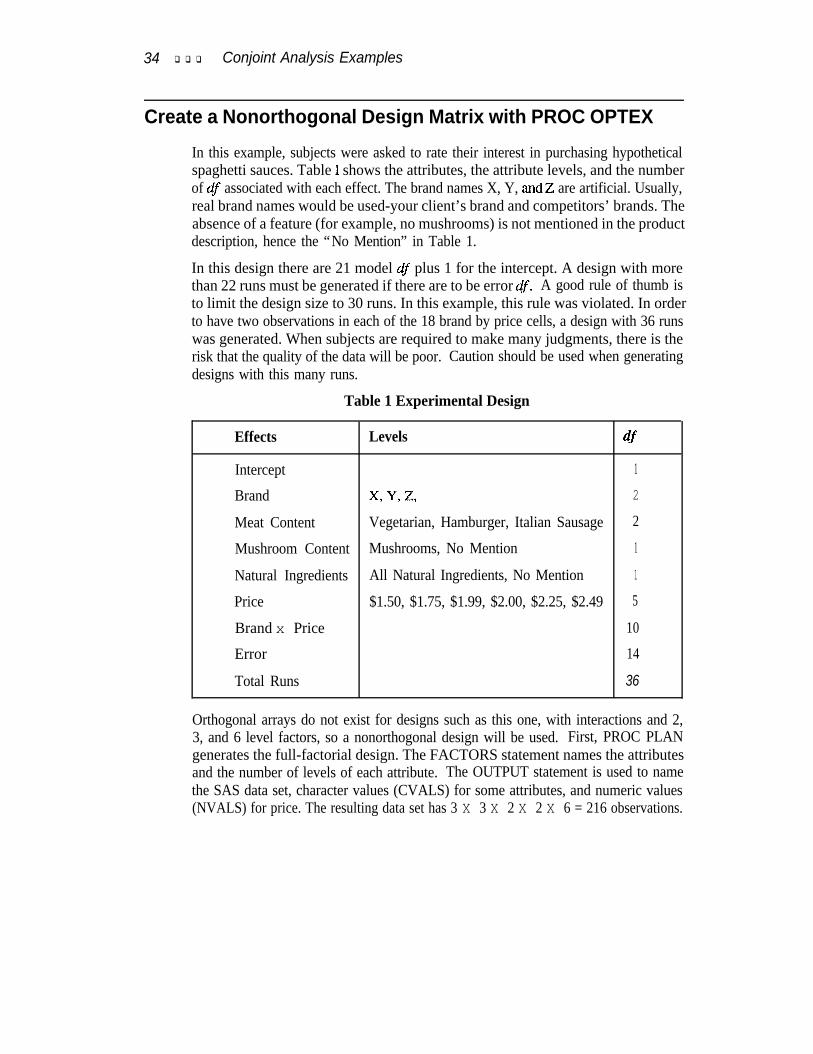
In this example, subjects were asked to rate their interest in purchasing hypotheticalspaghetti sauces. Table 1 shows the attributes, the attribute levels, and the numberof df associated with each effect. The brand names X, Y, andZ are artificial. Usually,real brand names would be used-your client’s brand and competitors’ brands. Theabsence of a feature (for example, no mushrooms) is not mentioned in the productdescription, hence the “No Mention” in Table 1.
In this design there are 21 model df plus 1 for the intercept. A design with morethan 22 runs must be generated if there are to be error df. A good rule of thumb isto limit the design size to 30 runs. In this example, this rule was violated. In orderto have two observations in each of the 18 brand by price cells, a design with 36 runswas generated. When subjects are required to make many judgments, there is therisk that the quality of the data will be poor. Caution should be used when generatingdesigns with this many runs.
Table 1 Experimental Design
Effects Levels df
Intercept 1
Brand x Y, z, 2
Meat Content Vegetarian, Hamburger, Italian Sausage 2
Mushroom Content Mushrooms, No Mention 1
Natural Ingredients All Natural Ingredients, No Mention 1
Price $1.50, $1.75, $1.99, $2.00, $2.25, $2.49 5
Brand x Price 10
Error 14
Total Runs 36
Orthogonal arrays do not exist for designs such as this one, with interactions and 2,3, and 6 level factors, so a nonorthogonal design will be used. First, PROC PLANgenerates the full-factorial design. The FACTORS statement names the attributesand the number of levels of each attribute. The OUTPUT statement is used to namethe SAS data set, character values (CVALS) for some attributes, and numeric values(NVALS) for price. The resulting data set has 3 X 3 X 2 X 2 X 6 = 216 observations.
Create a Nonorthogonal Design Matrix with PROC OPTEX q •I q 35
title 'Conjoint Analysis of Spaghetti Sauce Data';
* Generate a full-factorial design;proc plan ordered;
factors brand=3 meat=3 mushroom=2 natural=2 price=6 / noprintoutput out=designl
brand cvals=(‘X’ ‘Y’ fZ#)meat cvals=('Vegetarian' 'Hamburger 'Italian Sausage'mushroom cvals=('MushroomsP sNo Mention')natural cvals=('All Natural Ingredients' 'No Mention')price nvals=(1.50 1.75 1.99 2.00 2.25 2.49);
run ;quit;
Then a DATA step eliminates unrealistic combinations. Specifically, combinationsat $1.50 with meat and Italian Sausage with All Natural Ingredients are eliminated.This data set, with 162 observations, will be the candidate set for creating a nonor-thogonal design.
title 'Conjoint Analysis of Spaghetti Sauce Data';
* Exclude unrealistic combinations;data designa;
set designl;* Note, =: is the 'begins with' operator;if (meat =: 'Ham' or meat =: 'Ita') and price < 1.51
then delete;if meat =: 'Ita' and natural =: 'All' then delete;run:
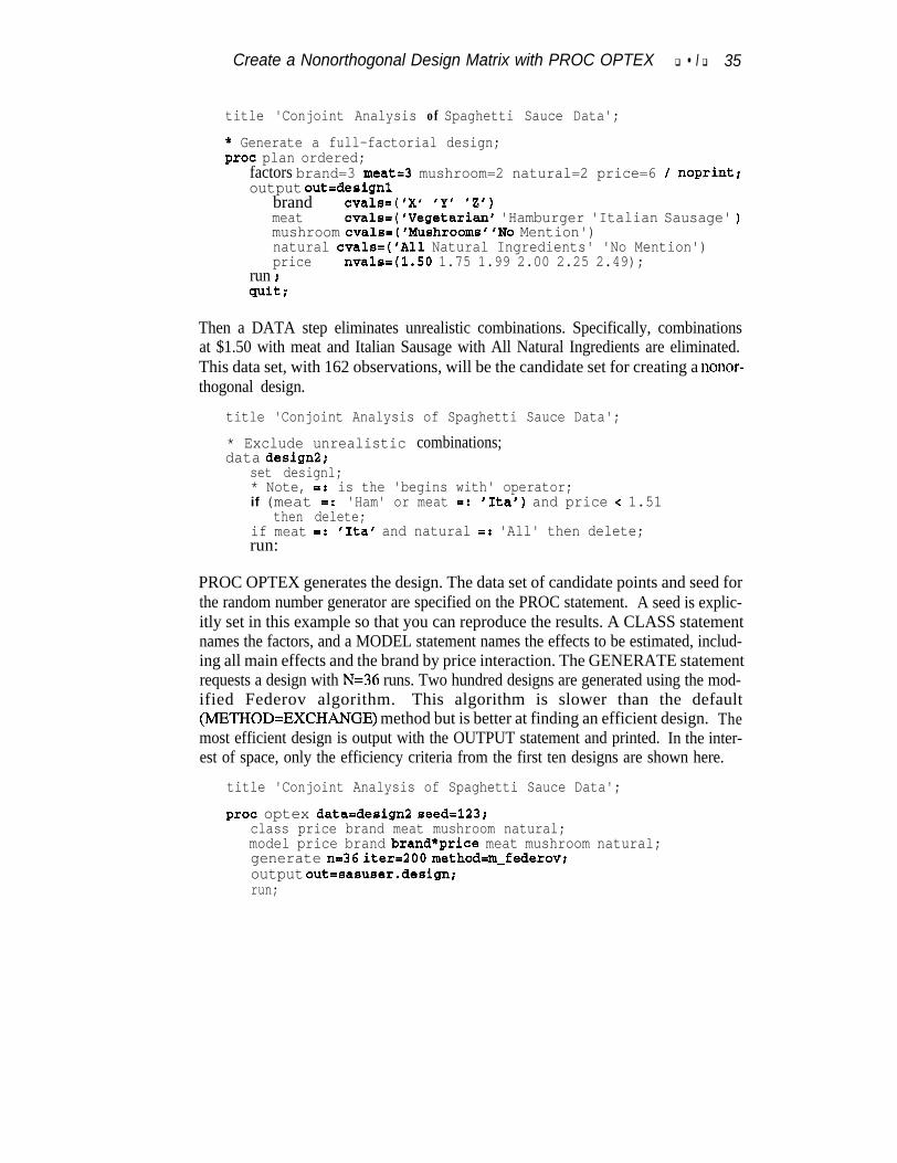
PROC OPTEX generates the design. The data set of candidate points and seed forthe random number generator are specified on the PROC statement. A seed is explic-itly set in this example so that you can reproduce the results. A CLASS statementnames the factors, and a MODEL statement names the effects to be estimated, includ-ing all main effects and the brand by price interaction. The GENERATE statementrequests a design with N=36 runs. Two hundred designs are generated using the mod-ified Federov algorithm. This algorithm is slower than the default(METHOD=EXCHANGE) method but is better at finding an efficient design. Themost efficient design is output with the OUTPUT statement and printed. In the inter-est of space, only the efficiency criteria from the first ten designs are shown here.
title 'Conjoint Analysis of Spaghetti Sauce Data';
proc optex data=design2 seed=123;class price brand meat mushroom natural;model price brand brand*price meat mushroom natural;generate nx36 iterG method=m-federov;output out=sasuser.design;run;
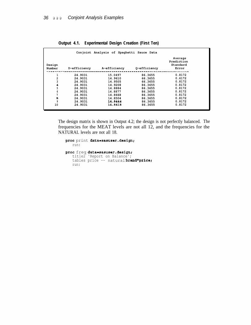
36 q q q Conjoint Analysis Examples
Output 4.1. Experimental Design Creation (First Ten)
Conjoint Analysis of Spaghetti Sauce Data
AveragePrediction
Design StandardNumber D-efficiency A-efficiency Q-efficiency Error------------------__----------------------------------------------------
1 24.9031 15.0497 86.3655 0.81722 24.9031 14.9610 66.3655 0.61723 24.9031 14.9505 66.3655 0.81724 24.9031 14.9208 86.3655 0.81725 24.9031 14.8884 86.3655 0.81726 24.9031 14.8877 86.3655 0.81727 24.9031 14.8668 86.3655 0.81728 24.9031 14.8504 86.3655 0.81729 24.9031 14.8444 86.3655 0.8172
10 24.9031 14.8418 86.3655 0.8172
The design matrix is shown in Output 4.2; the design is not perfectly balanced. Thefrequencies for the MEAT levels are not all 12, and the frequencies for theNATURAL levels are not all 18.
proc print data=sasuser.design;run:
proc freq data=sasuser.design:title2 'Report on Balance';tables price -- natural brand*price;run:
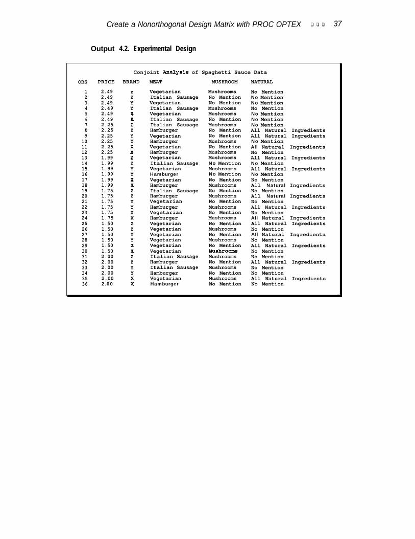
Create a Nonorthogonal Design Matrix with PROC OPTEX q q q 37
Output 4.2. Experimental Design
Conjoint Analysis of Spaghetti Sauce Data
OBS PRICE BRAND MEAT MUSHROOM NATURAL
1 2.49 z Vegetarian Mushrooms No Mention2 2.49 Z Italian Sausage No Mention No Mention3 2.49 Y Vegetarian No Mention No Mention4 2.49 Y Italian Sausage Mushrooms No Mention5 2.49 x Vegetarian Mushrooms No Mention6 2.49 x Italian Sausage No Mention No Mention7 2.25 Z Italian Sausage Mushrooms No Mention8 2.25 Z Hamburger No Mention All Natural Ingredients9 2.25 Y Vegetarian No Mention All Natural Ingredients
10 2.25 Y Hamburger Mushrooms No Mention11 2.25 x Vegetarian No Mention All Natural Ingredients12 2.25 x Hamburger Mushrooms No Mention13 1.99 2 Vegetarian Mushrooms All Natural Ingredients14 1.99 Z Italian Sausage No Mention No Mention15 1.99 Y Vegetarian Mushrooms All Natural Ingredients16 1.99 Y Hamburger No Mention No Mention17 1.99 x Vegetarian No Mention No Mention18 1.99 x Hamburger Mushrooms All Natural Ingredients19 1.75 Z Italian Sausage No Mention No Mention20 1.75 Z Hamburger Mushrooms All Natural Ingredients21 1.75 Y Vegetarian No Mention No Mention22 1.75 Y Hamburger Mushrooms All Natural Ingredients23 1.75 X Vegetarian No Mention No Mention24 1.75 X Hamburger Mushrooms All Natural Ingredients25 1.50 Z Vegetarian No Mention All Natural Ingredients26 1.50 Z Vegetarian Mushrooms No Mention27 1.50 Y Vegetarian No Mention All Natural Ingredienta28 1.50 Y Vegetarian Mushrooms No Mention29 1.50 X Vegetarian No Mention All Natural Ingredients30 1.50 X Vegetarian Nushrooms No Mention31 2.00 Z Italian Sausage Mushrooms No Mention32 2.00 Z Hamburger No Mention All Natural Ingredients33 2.00 Y Italian Sausage Mushrooms No Mention34 2.00 Y Hamburger No Mention No Mention35 2.00 X Vegetarian Mushrooms All Natural Ingredients36 2.00 X Hamburger No Mention No Mention
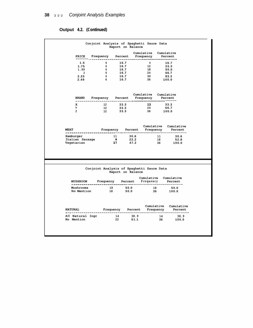
38 q q q Conjoint Analysis Examples
Output 4.2. (Continued)
Conjoint Analysis of Spaghetti Sauce DataReport on Balance
PRICE-------
1.51.751.99
22.252.49
Cumulative CumulativeFrequency Percent Frequency Percent
.___________________-------------------------6 16.7 6 16.76 16.7 12 33.36 16.7 18 50.06 16.7 24 66.76 16.7 30 83.36 16.7 36 100.0
Cumulative CumulativeBRAND Frequency Percent Frequency Percent____________________------------------------- ------X 12 33.3 12 33.3Y 12 33.3 24 66.7Z 12 33.3 36 100.0
Cumulative CumulativeMEAT Frequency Percent Frequency Percent________________________________________---------------------Hamburger 11 30.6 11 30.6Italian Sausage 8 22.2 19 52.8Vegetarian 17 47.2 36 100.0
Conjoint Analysis of Spaghetti Sauce DataReport on Balance
Cumulative CumulativeMUSHROOM Frequency Percent Frequency Percent____________________------------------------------------Mushrooms 18 50.0 18 50.0No Mention 18 50.0 36 100.0
Cumulative CumulativeNATURAL Frequency Percent Frequency Percent____________________------------------------------------------All Natural Ingr 14 38.9 14 38.9No Mention 22 61.1 36 100.0
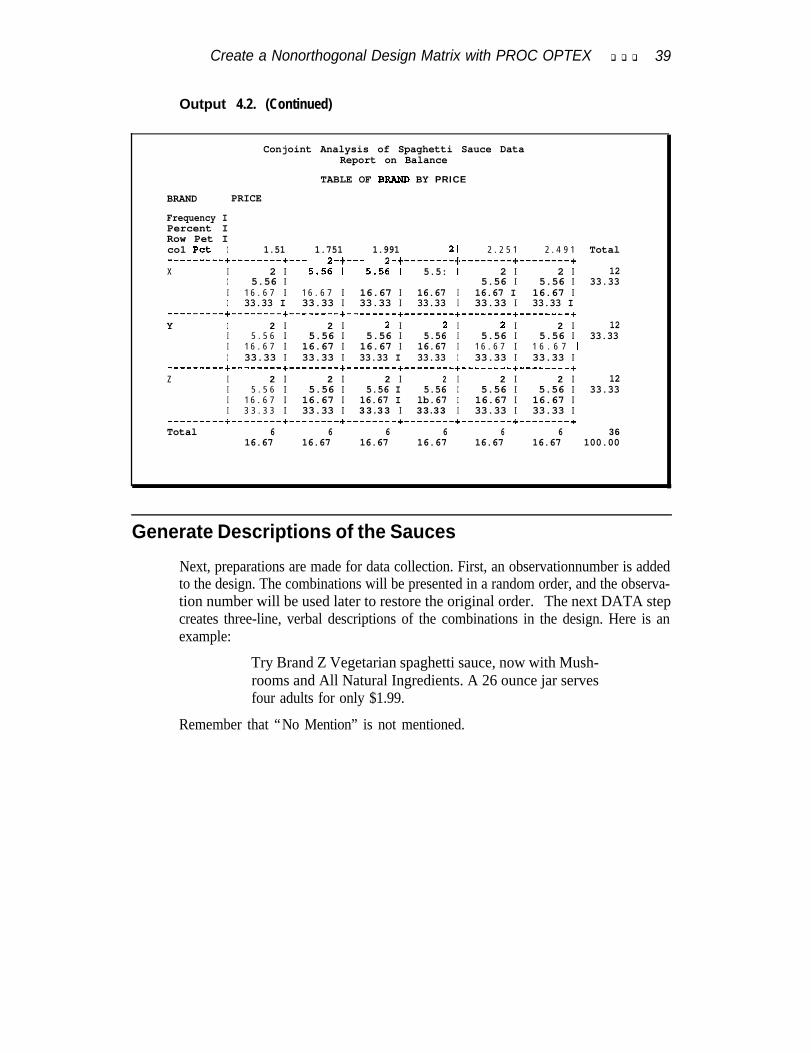
Create a Nonorthogonal Design Matrix with PROC OPTEX q q q 39
Output 4.2. (Continued)
Conjoint Analysis of Spaghetti Sauce DataReport on Balance
TABLE OF BRAND BY PRICEBRAND PRICE
Frequency IPercent IRow Pet Ico1 Pet I 1.51 1.751 1.991 al 2 . 2 5 1 2 . 4 9 1---------+--------+--------+--------+--------+--------+--------+
X I 2 I 5.5: I 5.5: I 5.5: I 2 I 2 II 5.56 I 5.56 I 5.56 II 1 6 . 6 7 I 1 6 . 6 7 I 16.67 I 16.67 I 16.67 I 16.67 II 33.33 I 33.33 I 33.33 I 33.33 I 33.33 I 33.33 I
---------+--------+--------+--------+--------+--------+--------+Y I 2 I 2 I 2 I 2 I 2 I 2 I
I 5 . 5 6 I 5.56 I 5.56 I 5.56 I 5.56 I 5.56 II 1 6 . 6 7 I 16.67 I 16.67 I 16.67 I 1 6 . 6 7 I 1 6 . 6 7 lI 33.33 I 33.33 I 33.33 I 33.33 I 33.33 I 33.33 I
---------+--------+--------+--------+--------+--------~--------+
Z I 2 I 2 I 2 I 2 I 2 I 2 II 5 . 5 6 I 5.56 I 5.56 I 5.56 I 5.56 I 5.56 II 1 6 . 6 7 I 16.67 I 16.67 I lb.67 I 16.67 I 16.67 II 3 3 . 3 3 I 33.33 I 33.33 I 33.33 I 33.33 I 33.33 I
---------+--------+---- ----+--------+--------+--------+----------+Total 6 6 6 6 6 6
16.67 16.67 16.67 16.67 16.67 16.67
Total
1233.33
1233.33
1233.33
36100.00
Generate Descriptions of the Sauces
Next, preparations are made for data collection. First, an observationnumber is addedto the design. The combinations will be presented in a random order, and the observa-tion number will be used later to restore the original order. The next DATA stepcreates three-line, verbal descriptions of the combinations in the design. Here is anexample:
Try Brand Z Vegetarian spaghetti sauce, now with Mush-rooms and All Natural Ingredients. A 26 ounce jar servesfour adults for only $1.99.
Remember that “No Mention” is not mentioned.
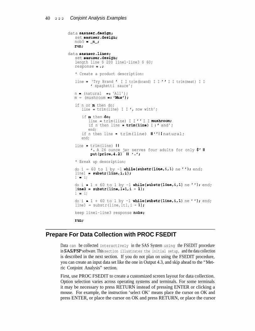
40 q q q Conjoint Analysis Examples
data sasuser.design;set sasuser.design;nob5 = -n-irunr
data sasuser.lines;set sasuser.design;length line $ 200 linel-line3 $ 60;response = .;
* Create a product description:
line = ‘Try Brand I I I trim(brand) I I ’ ’ I I trim(meat) I I’ spaghetti sauce’;
n = (natural =: ‘All’);m = (mushroom =: ‘MUS’);
if n or m then do;line = trim(line) I I #, now with’;
if RI then dOiline = trim(line) I I I B I I mU5hr00ltliif n then line = trim(line) I I ’ and’;end;
if n then line = trim(line) II ’ ’ II natural;end;
line = trim(line) I II. A 26 ounce jar serves four adults for only $’ IIput(price,4.2) II ‘es;
* Break up description;
do i = 60 to 1 by -1 while(substr(line,i,l) ne ’ ‘); end;line1 = substr(line,l,i);1 = i;
do i = 1 + 60 to 1 by -1 while(substr(line,i,l) ne ’ ‘)i end;1 ine2 = substr(line,l+l,i - 1);1 = i;
do i = 1 + 60 to 1 by -1 while(substr(line,i,l) ne ’ ‘)i end;line3 = substr(line,ltl,i - 1);
keep linel-line3 response nabs;
run;
Prepare For Data Collection with PROC FSEDIT
Data can be collected interactively in the SAS System using the FSEDIT procedurein SAS/FSP software. This section illustrates the initial setup, and the data collectionis described in the next section. If you do not plan on using the FSEDIT procedure,you can create an input data set like the one in Output 4.3, and skip ahead to the “Met-ric Conjoint Analysis” section.
First, use PROC FSEDIT to create a customized screen layout for data collection.Option selection varies across operating systems and terminals. For some terminalsit may be necessary to press RETURN instead of pressing ENTER or clicking amouse. For example, the instruction ‘select OK’ means place the cursor on OK andpress ENTER, or place the cursor on OK and press RETURN, or place the cursor
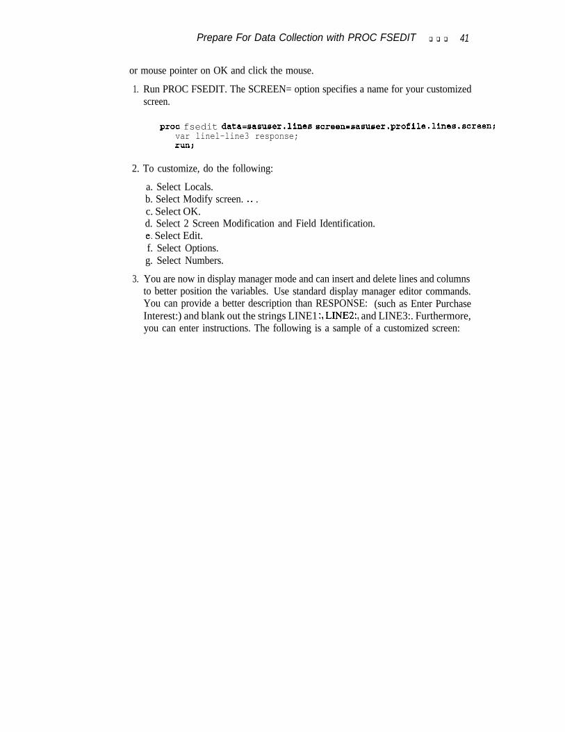
Prepare For Data Collection with PROC FSEDIT q q q 41
or mouse pointer on OK and click the mouse.
1. Run PROC FSEDIT. The SCREEN= option specifies a name for your customizedscreen.
proc fsedit data=sasuser.lines screen=sasuser.profile.lines.screen;var linel-line3 response;rUn;
2. To customize, do the following:
a. Select Locals.b. Select Modify screen. a. .c. Select OK.d. Select 2 Screen Modification and Field Identification.e. Select Edit.f. Select Options.g. Select Numbers.
3. You are now in display manager mode and can insert and delete lines and columnsto better position the variables. Use standard display manager editor commands.You can provide a better description than RESPONSE: (such as Enter PurchaseInterest:) and blank out the strings LINE1 :, LINE2:, and LINE3:. Furthermore,you can enter instructions. The following is a sample of a customized screen:
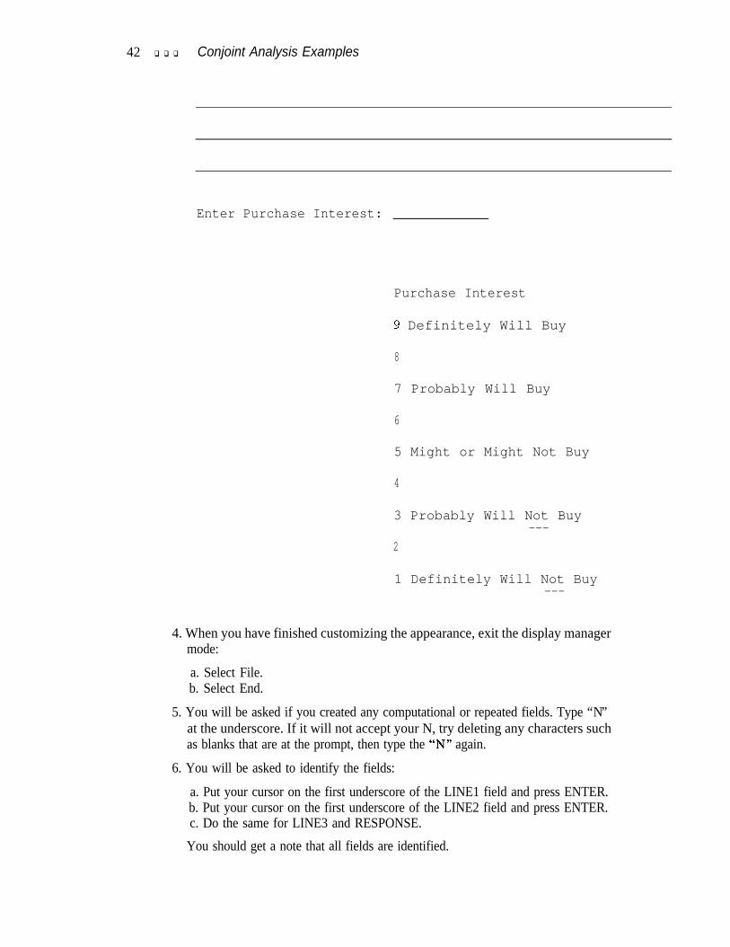
42 q q q Conjoint Analysis Examples
Enter Purchase Interest:
Purchase Interest
9 Definitely Will Buy
8
7 Probably Will Buy
6
5 Might or Might Not Buy
4
3 Probably Will Not Buy---
2
1 Definitely Will Not Buy---
4. When you have finished customizing the appearance, exit the display managermode:
a. Select File.b. Select End.
5. You will be asked if you created any computational or repeated fields. Type “N”at the underscore. If it will not accept your N, try deleting any characters suchas blanks that are at the prompt, then type the “N” again.
6. You will be asked to identify the fields:
a. Put your cursor on the first underscore of the LINE1 field and press ENTER.b. Put your cursor on the first underscore of the LINE2 field and press ENTER.c. Do the same for LINE3 and RESPONSE.
You should get a note that all fields are identified.
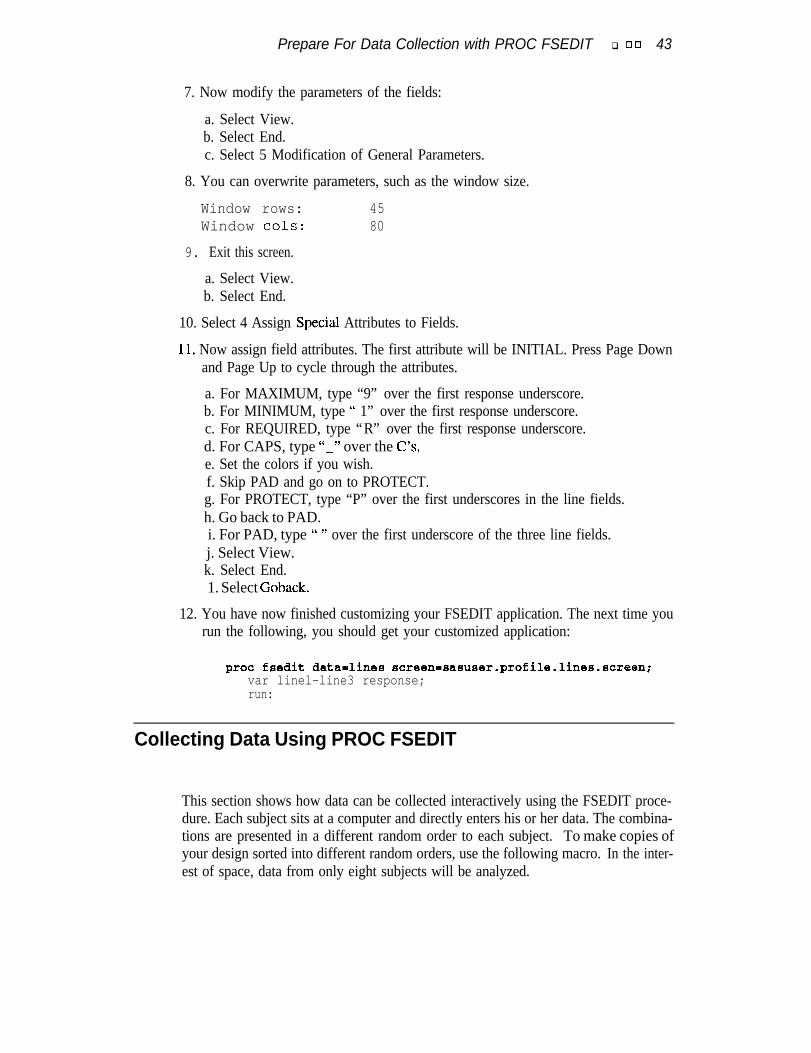
Prepare For Data Collection with PROC FSEDIT q 0 0 43
7. Now modify the parameters of the fields:
a. Select View.b. Select End.c. Select 5 Modification of General Parameters.
8. You can overwrite parameters, such as the window size.
Window rows: 45Window ~01s: 80
9. Exit this screen.
a. Select View.b. Select End.
10. Select 4 Assign SpeciaI Attributes to Fields.
11, Now assign field attributes. The first attribute will be INITIAL. Press Page Downand Page Up to cycle through the attributes.
a. For MAXIMUM, type “9” over the first response underscore.b. For MINIMUM, type “ 1” over the first response underscore.c. For REQUIRED, type “R” over the first response underscore.d. For CAPS, type “-” over the C’s,e. Set the colors if you wish.f. Skip PAD and go on to PROTECT.g. For PROTECT, type “P” over the first underscores in the line fields.h. Go back to PAD.i. For PAD, type “ ” over the first underscore of the three line fields.j. Select View.k. Select End.1. Select Goback.
12. You have now finished customizing your FSEDIT application. The next time yourun the following, you should get your customized application:
proc fsedit datadines screen=sasuser.profile.line0.acreen;var linel-line3 response;run:
Collecting Data Using PROC FSEDIT
This section shows how data can be collected interactively using the FSEDIT proce-dure. Each subject sits at a computer and directly enters his or her data. The combina-tions are presented in a different random order to each subject. To make copies ofyour design sorted into different random orders, use the following macro. In the inter-est of space, data from only eight subjects will be analyzed.
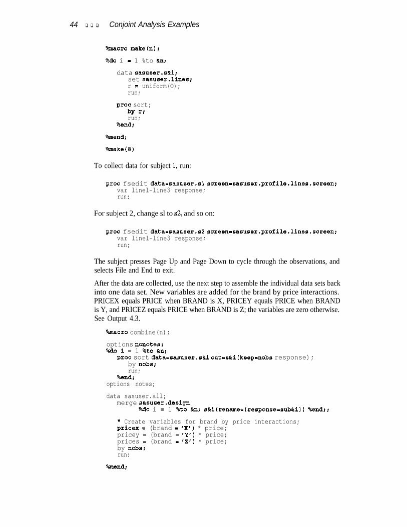
44 q q q Conjoint Analysis Examples
"%macro make(n);
O%ao i = 1 %to &n;
data sasuser.s&i;set sasuser.lines;r = uniform(O);run;
proc sort;by rtrun;
%endt
Omena;
&take(B)
To collect data for subject 1, run:
proc fsedit data=sasuser.sl screen=sasuser.profile.lines.screen;var linel-line3 response;run:
For subject 2, change sl to ~2, and so on:
proc fsedit data=sasuser.sS screen=sasuser.profile.lines.screen;var linel-line3 response;run;
The subject presses Page Up and Page Down to cycle through the observations, andselects File and End to exit.
After the data are collected, use the next step to assemble the individual data sets backinto one data set. New variables are added for the brand by price interactions.PRICEX equals PRICE when BRAND is X, PRICEY equals PRICE when BRANDis Y, and PRICEZ equals PRICE when BRAND is Z; the variables are zero otherwise.See Output 4.3.
%macro combine(n);
options nonotes;%a0 i = 1 %to 6rn;
proc sort data=sasuser.s&i out=s&i(keep=nobs response);by nabs;run;
%end;options notes;
data sasuser.all;merge sasuser.design
O%do i = 1 %to &n; s&i(rename=(response=sub&i)) %end;;
* Create variables for brand by price interactions;pricex I (brand = 'X') * price;pricey = (brand = 'Y') * price;prices = (brand = '2') * price;by nobs;run:
%mend;
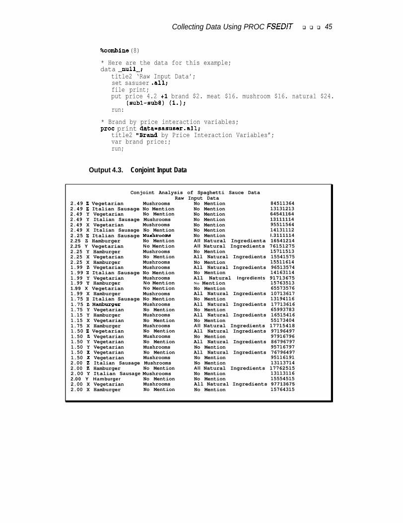
Collecting Data Using PROC FSEDIT q q q 45
%combine (8)
* Here are the data for this example;data -null-;
title2 ‘Raw Input Data’;set sasuser .all;file print;put price 4.2 +l brand $2. meat $16. mushroom $16. natural $24.
(subl-sub8) (1.);run:
* Brand by price interaction variables;proc print data=sasuser.all;
title2 “Brand by Price Interaction Variables”;var brand price:;run;
Output 4.3. Conjoint Input Data
Conjoint Analysis of Spaghetti Sauce DataRaw Input Data
2.49 Z Vegetarian Mushrooms No Mention 845113642.49 2 Italian Sausage No Mention No Mention 131312132.49 Y Vegetarian No Mention No Mention 645411642.49 Y Italian Sausage Mushrooms No Mention 131111142.49 X Vegetarian Mushrooms No Mention 955115642.49 X Italian Sausage No Mention No Mention 141311122.25 Z Italian Sausage Mushroonrs No Mention I.31111142.25 2 Hamburger No Mention All Natural Ingredienta 165412142.25 Y Vegetarian No Mention All Natural Ingredients 761512752.25 Y Hamburger Mushrooms No Mention 157115132.25 X Vegetarian No Mention All Natural Ingredients 155415752.25 X Hamburger Mushrooms No Mention 155116141.99 2 Vegetarian Mushrooms All Natural Ingredients 965135741.99 2 Italian Sausage No Mention No Mention 141631141.99 Y Vegetarian Mushrooms All Natural Ingredients 917136751.99 Y Hamburger No Mention NO Mention 157635131.99 X Vegetarian No Mention No Mention 655735761.99 X Hamburger Mushrooms All Natural Ingredients 107136171.75 !Z Italian Sausage No Mention No Mention 131941161.75 2 Hamburger Mushrooms All Natural Ingredients 177136161.75 Y Vegetarian No Mention No Mention 659937831.15 Y Hamburger Mushrooms All Natural Ingredients 165154161.15 X Vegetarian No Mention No Mention 551734041.75 X Hamburger Mushrooms All Natural Ingredients 177154181.50 2 Vegetarian No Mention All Natural Ingredients 971964971.50 Z Vegetarian Mushrooms No Mention 979167961.50 Y Vegetarian No Mention All Natural Ingredients 867967971.50 Y Vegetarian Mushrooms No Mention 957167971.50 X Vegetarian No Mention All Natural Ingredients 767964971.50 X Vegetarian Mushrooms No Mention 951161912.00 z Italian Sausage Mushrooms No Mention 131137142.00 2 Hamburger No Mention All Natural Ingredients 177625152.00 Y Italian Sausage Mushrooms No Mention 131131162.00 Y Hamburger No Mention No Mention 155545152.00 X Vegetarian Mushrooms All Natural Ingredients 977136752.00 X Hamburger No Mention No Mention 15764315
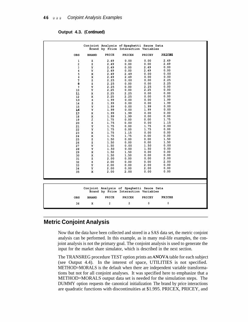
4 6 q q q Conjoint Analysis Examples
Output 4.3. (Continued)
Conjoint Analysis of Spaghetti Sauce DataBrand by Price Interaction Variables
OBS BRAND PRICE PRICEX PRICEY PRICE2
1 Z 2.49 0.00 0.00 2.492 Z 2.49 0.00 0.00 2.493 Y 2.49 0.00 2.49 0.004 Y 2.49 0.00 2.49 0.005 X 2.49 2.49 0.00 0.006 X 2.49 2.49 0.00 0.007 Z 2.25 0.00 0.00 2.258 Z 2.25 0.00 0.00 2.259 Y 2.25 0.00 2.25 0.00
10 Y 2.25 0.00 2.25 0.0011 X 2.25 2.25 0.00 0.0012 X 2.25 2.25 0.00 0.0013 Z 1.99 0.00 0.00 1.9914 Z 1.99 0.00 0.00 1.9915 Y 1.99 0.00 1.99 0.0016 Y 1.99 0.00 1.99 0.0017 X 1.99 1.99 0.00 0.0018 X 1.99 1.99 0.00 0.0019 Z 1.75 0.00 0.00 1.7520 Z 1.75 0.00 0.00 1.1521 Y 1.75 0.00 1.75 0.0022 Y 1.75 0.00 1.75 0.0023 X 1.75 1.15 0.00 0.0024 X 1.75 1.75 0.00 0.0025 Z 1.50 0.00 0.00 1.5026 Z 1.50 0.00 0.00 1.5027 Y 1.50 0.00 1.50 0.0028 Y 1.50 0.00 1.50 0.0029 X 1.50 1.50 0.00 0.0030 X 1.50 1.50 0.00 0.0031 Z 2.00 0.00 0.00 2.0032 Z 2.00 0.00 0.00 2.0033 Y 2.00 0.00 2.00 0.0034 Y 2.00 0.00 2.00 0.0035 X 2.00 2.00 0.00 0.00
Conjoint Analysis of Spaghetti Sauce DataBrand by Price Interaction Variables
OBS BRAND PRICE PRICEX PRICEY PRICEZ
36 X 2 2 0 0
Metric Conjoint Analysis
Now that the data have been collected and stored in a SAS data set, the metric conjointanalysis can be performed. In this example, as in many real-life examples, the con-joint analysis is not the primary goal. The conjoint analysis is used to generate theinput for the market share simulator, which is described in the next section.
The TRANSREG procedure TEST option prints an ANOVA table for each subject(see Output 4.4). In the interest of space, UTILITIES is not specified.METHOD=MORALS is the default when there are independent variable transforma-tions but not for all conjoint analyses. It was specified here to emphasize that aMETHOD=MORALS output data set is needed for the simulation steps. TheDUMMY option requests the canonical initialization The brand by price interactionsare quadratic functions with discontinuities at $1.995. PRICEX, PRICEY, and
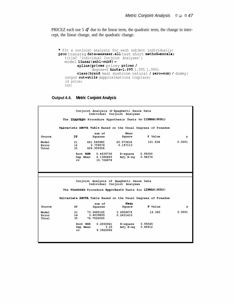
Metric Conjoint Analysis 0 q 0 47
PRICEZ each use 5 df due to the linear term, the quadratic term, the change in inter-cept, the linear change, and the quadratic change.
* Fit a conjoint analysis for each subject individually;proc transreg data=sasuser.all test short method=morals;
title2 ‘Individual Conjoint Analyses’;model lineartsubl-sub81 =
splinetpricex pricey price2 /degree=2 knotw1.995 1.995 1.995)
class(brand meat mushroom natural / zero=sum) / dummy;output out=utils dapproximations ireplace;id price;run;
Output 4.4. Metric Conjoint Analysis
Conjoint Analysis of Spaghetti Sauce DataIndividual Conjoint Analyses
The TRANSREQ Procedure Hypothesis Tests for LINEAR(SUB1)
Unfvariate ANOVA Table Based on the Usual Degrees of Freedom
sum of MeanSource DF Squares Square F Value P
Model 21 421.545980 20.073618 101.838 0.0001Error 14 2.759576 0.197113Total 35 424.305556
Root WE 0.4439736 R-square 0.99350Dep Mean 4.1388889 Adj R-sq 0.98374cv 10.726878
Conjoint Analysis of Spaghetti Sauce DataIndividual Conjoint Analyses
The TRANSRBG Procedure Hypothesis Tests for LINRAR(SUB2)
Unlvariate ANOVA Table Based on the Usual Degrees of Freedom
Source
ModelErrorTotal
sum of MeWIDF Squares Square F Value P
21 73.3460145 3.4926674 14.365 0.0001I4 3.4039855 0.243141035 76.7500000
Root MSE 0.4930941 R-square 0.95565Dep Mean 5.25 Adj R-aq 0.88912cv 9.3922692
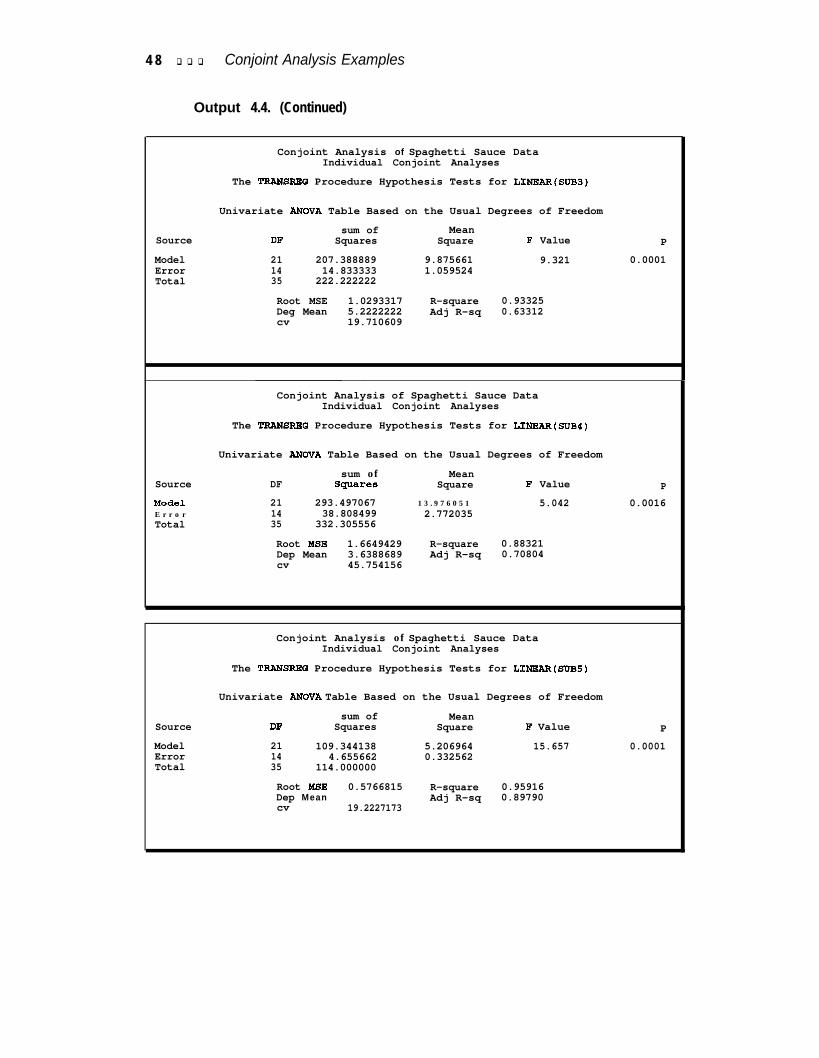
4 8 q q q Conjoint Analysis Examples
Output 4.4. (Continued)
Conjoint Analysis of Spaghetti Sauce DataIndividual Conjoint Analyses
The TRANSREQ Procedure Hypothesis Tests for LINEAR(SUB3)
Univariate ANOVA Table Based on the Usual Degrees of Freedom
Source
ModelErrorTotal
sum of MeanDF Squares Square F Value P
21 207.388889 9.875661 9.321 0.000114 14.833333 1.05952435 222.222222
Root MSE 1.0293317 R-square 0.93325Deg Mean 5.2222222 Adj R-sq 0.63312cv 19.710609
Conjoint Analysis of Spaghetti Sauce DataIndividual Conjoint Analyses
The TRANSRRO Procedure Hypothesis Tests for LINSAR(SUB4)
Univariate ANOVA Table Based on the Usual Degrees of Freedom
Source
ModelE r r o rTotal
sum of MeanDF Squarea Square F Value P21 293.497067 13 .976051 5.042 0.001614 38.808499 2.77203535 332.305556
Root MSE 1.6649429 R-square 0.88321Dep Mean 3.6388689 Adj R-sq 0.70804cv 45.754156
Conjoint Analysis of Spaghetti Sauce DataIndividual Conjoint Analyses
The TRANSRRO Procedure Hypothesis Tests for LINEAR(SUB5)
Univariate ANOVA Table Based on the Usual Degrees of Freedom
Source
ModelErrorTotal
sum of MeanDF Squares Square F Value P
21 109.344138 5.206964 15.657 0.000114 4.655662 0.33256235 114.000000
Root MSE 0.5766815 R-square 0.95916Dep Mean Adj R-sq 0.89790cv 19.2227173
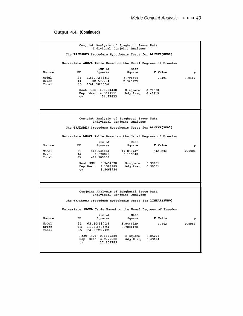
Metric Conjoint Analysis 0 0 0 49
Output 4.4. (Continued)
Conjoint Analysis of Spaghetti Sauce DataIndividual Conjoint Analyses
The TRANSRBQ Procedure Hypothesis Tests for LINEAR(SUB6)
Univarlate ANOVA Table Based on the Usual Degrees of Freedom
Source
ModelErrorTotal
sum of MeanDF Squares Square F Value P
21 121.727851 5.796564 2.491 0.041714 32.577704 2.32697935 154.305556
Root USE 1.5254438 R-square 0.78888Dep Mean 4.3611111 Adj R-sq 0.47219cv 34.97833
Conjoint Analysis of Spaghetti Sauce DataIndividual Conjoint Analyses
The TRANSRBC Procedure Hypothesis Tests for LINRAR(SUB7)
Univarlate ANOVA Table Based OII the Usual Degrees of Freedom
Source
ModelErrorTotal
sum of MeanDF Squares Square F Value P
21 416.634683 19.839747 166.234 0.000114 1.670872 0.11934835 418.305556
Root MSE 0.3454678 R-square 0.99601Dep Mean 4.1388889 Adj R-sq 0.99001cv 8.3468734
Conjoint Analysis of Spaghetti Sauce DataIndividual Conjoint Analyses
The TRANSREO Procedure Hypothesis Tests for LINEAR(SUB8)
Univariate ANOVA Table Based on the Usual Degrees of Freedom
Source
ModelErrorTotal
sum of MeanDF Squares Square P Value P21 63.9343728 3.0444939 3.862 0.006214 11.0378494 0.788417835 74.9722222
Root WE 0.8879289 R-square 0.85277Dep Mean 4.9722222 Adj R-sq 0.63194cv 17.857789
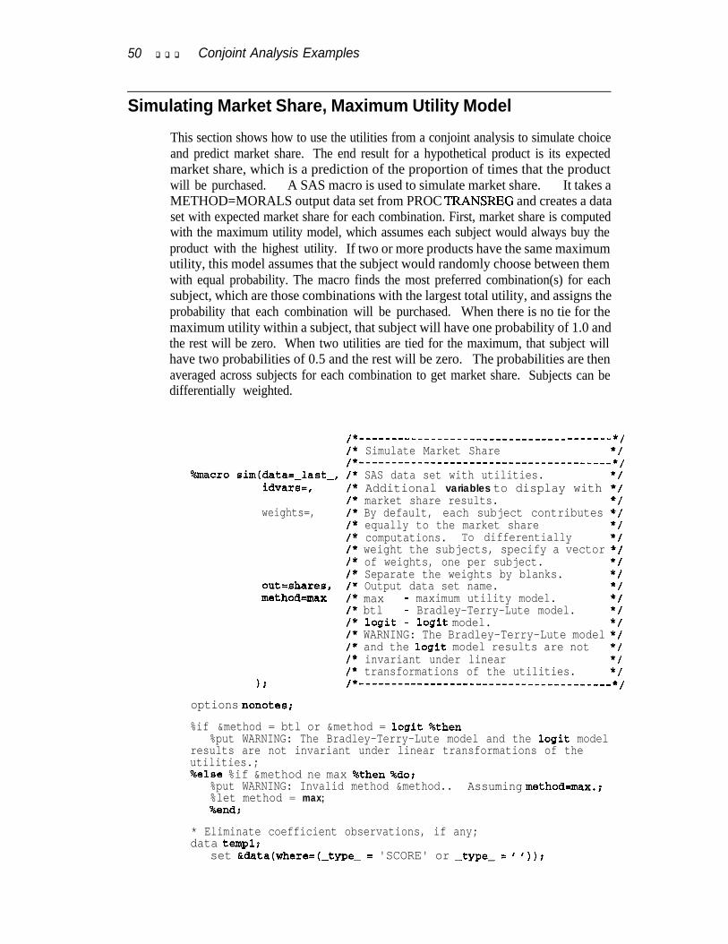
50 q q q Conjoint Analysis Examples
Simulating Market Share, Maximum Utility Model
This section shows how to use the utilities from a conjoint analysis to simulate choiceand predict market share. The end result for a hypothetical product is its expectedmarket share, which is a prediction of the proportion of times that the productwill be purchased. A SAS macro is used to simulate market share. It takes aMETHOD=MORALS output data set from PROC TRANSREG and creates a dataset with expected market share for each combination. First, market share is computedwith the maximum utility model, which assumes each subject would always buy theproduct with the highest utility. If two or more products have the same maximumutility, this model assumes that the subject would randomly choose between themwith equal probability. The macro finds the most preferred combination(s) for eachsubject, which are those combinations with the largest total utility, and assigns theprobability that each combination will be purchased. When there is no tie for themaximum utility within a subject, that subject will have one probability of 1.0 andthe rest will be zero. When two utilities are tied for the maximum, that subject willhave two probabilities of 0.5 and the rest will be zero. The probabilities are thenaveraged across subjects for each combination to get market share. Subjects can bedifferentially weighted.
/*-------------------------------- ------- *//* Simulate Market Share */1" ---------------------------------------*/
%macro sim(data=-last-, /* SAS data set with utilities. */idvars-, /* Additional variables to display with */
/* market share results. */weights=, /* By default, each subject contributes */
/* equally to the market share *//* computations. To differentially "//* weight the subjects, specify a vector *//* of weights, one per subject. *//* Separate the weights by blanks. "/
outnshares, /* Output data set name. */methodrmax /* max - maximum utility model. */
/" btl - Bradley-Terry-Lute model. "//* logit - logit model. *//* WARNING: The Bradley-Terry-Lute model *//* and the logit model results are not *//* invariant under linear *//* transformations of the utilities. */
1 ; /* ---------------------------------------*~
options nonotes;
%if &method = btl or &method = logit %then%put WARNING: The Bradley-Terry-Lute model and the logit model
results are not invariant under linear transformations of theutilities.;%else %if &method ne max %then %do;
%put WARNING: Invalid method &method.. Assuming method=max.;%let method = max;%end;
* Eliminate coefficient observations, if any;data templ;
set &data(where=(-type- = 'SCORE' or -type- = ' I));
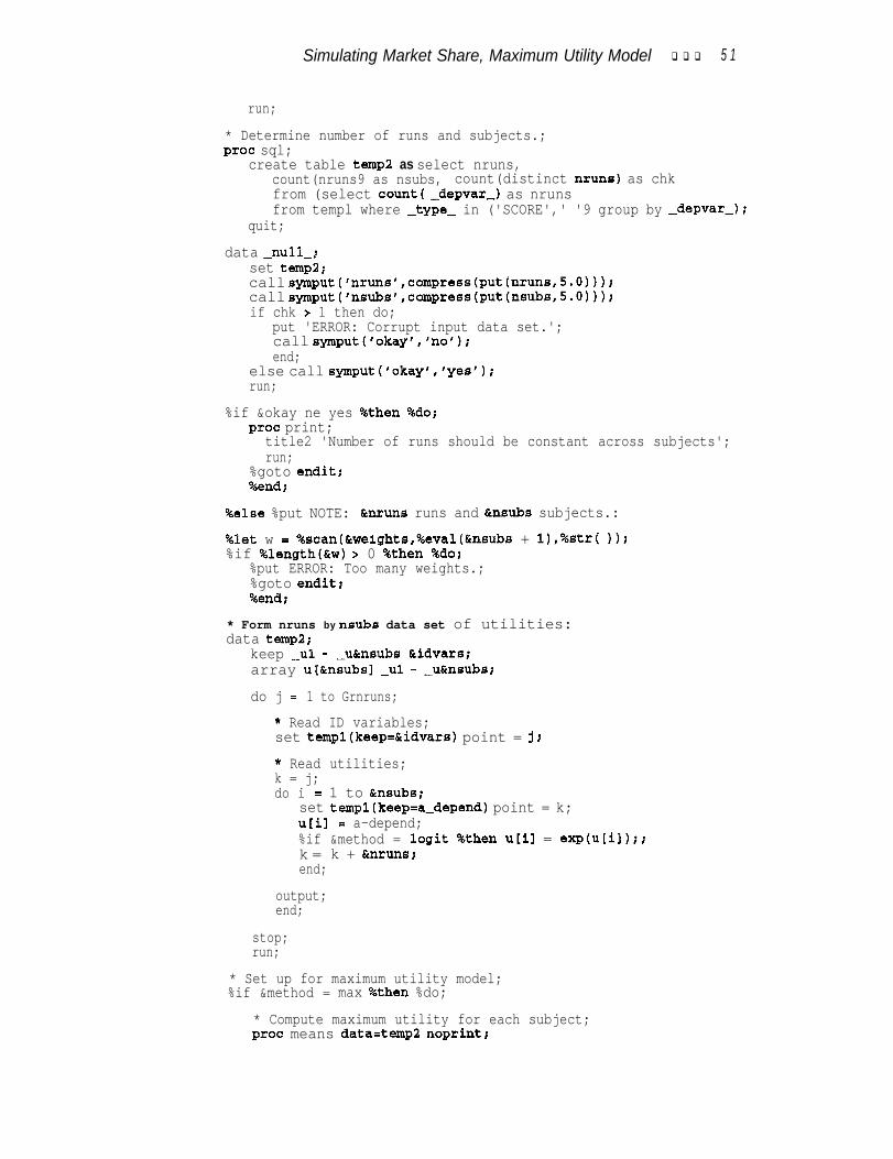
Simulating Market Share, Maximum Utility Model q q q 5 1
run;
* Determine number of runs and subjects.;proc sql;
create table templ as select nruns,count(nruns9 as nsubs, count(distinct nruns9 as chkfrom (select count( -depvar-9 as nrunsfrom templ where -type- in ('SCORE',' '9 group by -depvar.J;
quit;
data -null-;set temp2;call symput(fnrunsP,compress(put(nruns,5.0999;call symput('nsubs',compress(put(nsubs,5.0999;if chk > 1 then do;
put 'ERROR: Corrupt input data set.';call symput('okay','no');end;
else call symput('okay','yes');run;
%if &okay ne yes %then %do;proc print;
title2 'Number of runs should be constant across subjects';run;
%goto endit;%end;
%else %put NOTE: Grnruns runs and ansubs subjects.:
%let w = %scan(&weights,%eval(&nsubs + l),%str( 9);%if %length(&w) > 0 %then "%do;
%put ERROR: Too many weights.;%goto endit;%end;
* Form nruns by nsubs data set of utilities:data temp2;
keep -ul - -u&nsubs Gridvars;array u[&nsubsl -ul - -u&nsubs;
do j = 1 to Grnruns;
* Read ID variables;set templ(keep=hidvars) point = j;
* Read utilities;k = j;do i = 1 to ansubs;
set templ(keep=a-depend) point = k;u[il = a-depend;%if &method = logit %then u[il = exp(uLil9;;k = k + Grnruns;end;
output;end;
stop;run;
* Set up for maximum utility model;%if &method = max %then %do;
* Compute maximum utility for each subject;proc means data=temp2 noprint;
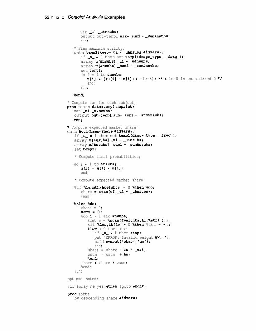
52 o q q ConjointAnalysis Examples
var -ul--u&nsubs;output out-templ max=-sum1 - -sum&nsubs;run:
* Flag maximum utility;data temp2(keep=-ul - -u&nsubs Gridvars);
if -n- = 1 then set templ(drop=-type--free);array u[&nsubsl -ul - -u&nsubs;array m[&nsubsl -sum1 - -sum&nsubs;set temp2;do i = 1 to Gmsubs;
util = ((u[il - m[i]) > -le-8); /* < le-8 is considered 0 */end;
run:
%end;
* Compute sum for each subject;proc means data=temp2 noprint;
var -ul--uLnsubs;output out=templ sum=-sum1 - -sumtnsubs;runi
* Compute expected market share;data Cout(keep=share Gridvars);
if -n- = 1 then set templ(drop=-type--free);array ut&nsubsl -ul - -u&nsubs;array m[&nsubs] -sum1 - -sum&nsubs;set temp2;
* Compute final probabilities;
do i = 1 to Grnsubs;u[il = u[il / m[il;end;
* Compute expected market share;
%if %length(&weights) = 0 %then "%do;share = meantof -ul - -u&nsubs);%end;
%else O%do;share = 0;wsum = 0;%do i = 1 %to ansubs;
%let w = %scan(kweights,&i,%str( ));%if %length(&w) = 0 %then %let w = .;if 6rw < 0 then do;
if -n- z 1 then stoptput "ERROR: Invalid weight a~..";call symput('okay','no');end;
share = share + &w * -u&i;wsum = wsum + 6rw;%end;
share = share / wsum;%end;
run:
options notes;
%if &okay ne yes %then %goto endit;
proc sort;by descending share aidvars;
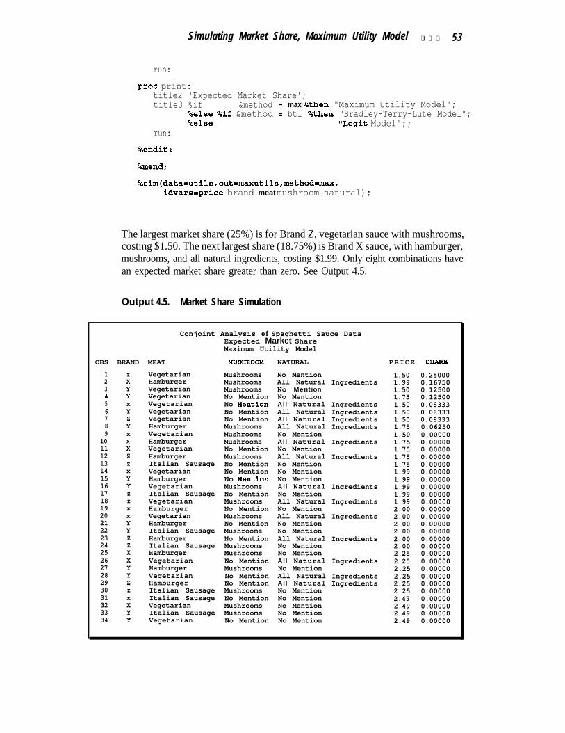
Simulating Market Share, Maximum Utility Model q q q 53
run:
proc print:title2 'Expected Market Share';title3 %if &method = max %then "Maximum Utility Model";
%else &if &method = btl %then "Bradley-Terry-Lute Model";%else "Logit Model";;
run:
%endit:
%mend;
%sim(data=utils,out=maxutils,method=max,idvars=price brand meat mushroom natural);
The largest market share (25%) is for Brand Z, vegetarian sauce with mushrooms,costing $1.50. The next largest share (18.75%) is Brand X sauce, with hamburger,mushrooms, and all natural ingredients, costing $1.99. Only eight combinations havean expected market share greater than zero. See Output 4.5.
Output 4.5. Market Share Simulation
Conjoint Analysis of Spaghetti Sauce DataExpected Market ShareMaximum Utility Model
OBS BRAND MEAT MUSHR00M NATURAL PRICE SHARE
1 z Vegetarian Mushrooms No Mention 1.50 0.250002 X Hamburger Mushrooms All Natural Ingredients 1.99 0.167503 Y Vegetarian Mushrooms No Mention 1.50 0.125004 Y Vegetarian No Mention No Mention 1.75 0.125005 x Vegetarian No ldention All Natural Ingredients 1.50 0.083336 Y Vegetarian No Mention All Natural Ingredients 1.50 0.083337 Z Vegetarian No Mention All Natural Ingredients 1.50 0.083338 Y Hamburger Mushrooms All Natural Ingredients 1.75 0.062509 x Vegetarian Mushrooms No Mention 1.50 0.00000
10 x Hamburger Mushrooms All Natural Ingredients 1.75 0.0000011 X Vegetarian No Mention No Mention 1.75 0.0000012 Z Hamburger Mushrooms All Natural Ingredients 1.75 0.0000013 z Italian Sausage No Mention No Mention 1.75 0.0000014 x Vegetarian No Mention No Mention 1.99 0.0000015 Y Hamburger No Mention No Mention 1.99 0.0000016 Y Vegetarian Mushrooms All Natural Ingredients 1.99 0.0000017 z Italian Sausage No Mention No Mention 1.99 0.0000018 z Vegetarian Mushrooms All Natural Ingredients 1.99 0.0000019 x Hamburger No Mention No Mention 2.00 0.0000020 x Vegetarian Mushrooms All Natural Ingredients 2.00 0.0000021 Y Hamburger No Mention No Mention 2.00 0.0000022 Y Italian Sausage Mushrooms No Mention 2.00 0.0000023 Z Hamburger No Mention All Natural Ingredients 2.00 0.0000024 Z Italian Sausage Mushrooms No Mention 2.00 0.0000025 X Hamburger Mushrooms No Mention 2.25 0.0000026 X Vegetarian No Mention All Natural Ingredients 2.25 0.0000027 Y Hamburger Mushrooms No Mention 2.25 0.0000028 Y Vegetarian No Mention All Natural Ingredients 2.25 0.0000029 Z Hamburger No Mention All Natural Ingredients 2.25 0.0000030 z Italian Sausage Mushrooms No Mention 2.25 0.0000031 x Italian Sausage No Mention No Mention 2.49 0.0000032 X Vegetarian Mushrooms No Mention 2.49 0.0000033 Y Italian Sausage Mushrooms No Mention 2.49 0.0000034 Y Vegetarian No Mention No Mention 2.49 0.00000
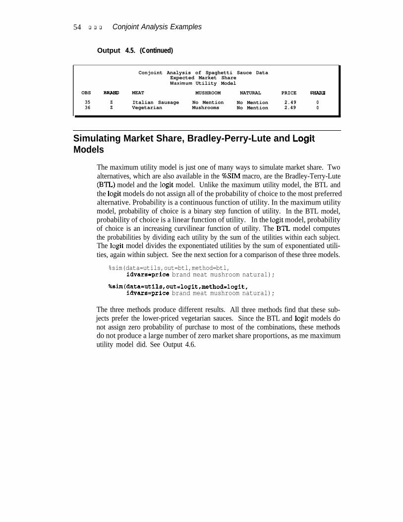
54 q q q Conjoint Analysis Examples
Output 4.5. (Continued)
Conjoint Analysis of Spaghetti Sauce DataExpected Market ShareMaximum Utility Model
OBS BRAND MEAT MUSHROOM NATURAL PRICE SHARE
35 Z Italian Sausage No Mention No Mention 2.49 036 Z Vegetarian Mushrooms No Mention 2.49 0
Simulating Market Share, Bradley-Perry-Lute and LogitModels
The maximum utility model is just one of many ways to simulate market share. Twoalternatives, which are also available in the %SIM macro, are the Bradley-Terry-Lute(BTL) model and the logit model. Unlike the maximum utility model, the BTL andthe logit models do not assign all of the probability of choice to the most preferredalternative. Probability is a continuous function of utility. In the maximum utilitymodel, probability of choice is a binary step function of utility. In the BTL model,probability of choice is a linear function of utility. In the logit model, probabilityof choice is an increasing curvilinear function of utility. The BTL model computesthe probabilities by dividing each utility by the sum of the utilities within each subject.The logit model divides the exponentiated utilities by the sum of exponentiated utili-ties, again within subject. See the next section for a comparison of these three models.
%sim(data=utils,out=btl,method=btl,idvarskprice brand meat mushroom natural);
%sim(data=utils,out=logit,method=logit,idvarseprice brand meat mushroom natural);
The three methods produce different results. All three methods find that these sub-jects prefer the lower-priced vegetarian sauces. Since the BTL and logit models donot assign zero probability of purchase to most of the combinations, these methodsdo not produce a large number of zero market share proportions, as me maximumutility model did. See Output 4.6.
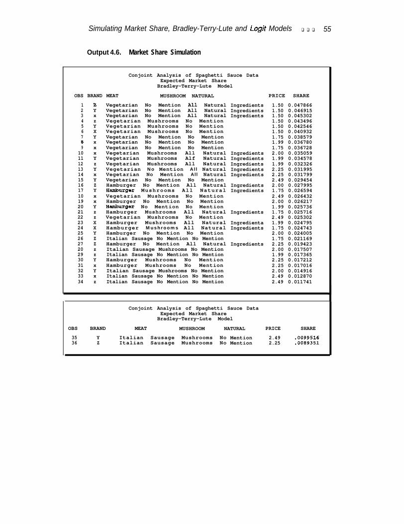
Simulating Market Share, Bradley-Terry-Lute and Logit Models q q q 55
Output 4.6. Market Share Simulation
Conjoint Analysis of Spaghetti Sauce DataExpected Market Share
Bradley-Terry-Lute Model
OBS BRAND MEAT MUSHROOM NATURAL PRICE SHARE
1 2 Vegetarian No Mention All Natural Ingredients 1.50 0.0478662 Y Vegetarian No Mention All Natural Ingredients 1.50 0.0469153 x Vegetarian No Mention All Natural Ingredients 1.50 0.0453024 z Vegetarian Mushrooms No Mention 1.50 0.0434965 Y Vegetarian Mushrooms No Mention 1.50 0.0425466 X Vegetarian Mushrooms No Mention 1.50 0.0409327 Y Vegetarian No Mention No Mention 1.75 0.0385790 x Vegetarian No Mention No Mention 1.99 0.0367809 x Vegetarian No Mention No Mention 1.75 0.036728
10 x Vegetarian Mushrooms All Natural Ingredients 2.00 0.03505911 Y Vegetarian Mushrooms Alf Natural Ingredients 1.99 0.03457812 z Vegetarian Mushrooms All Natural Ingredients 1.99 0.03232613 Y Vegetarian No Mention All Natural Ingredients 2.25 0.03199514 x Vegetarian No Mention All Natural Ingredients 2.25 0.03179915 Y Vegetarian No Mention No Mention 2.49 0.02945416 Z Hamburger No Mention All Natural Ingredients 2.00 0.02799517 Y I-kmhurger Mushrooms All Natural Ingredients 1.75 0.02659410 x Vegetarian Mushrooms No Mention 2.49 0.02643219 x Hamburger No Mention No Mention 2.00 0.02621720 Y Hamburger No Mention No Mention 1.99 0.02573621 z Hamburger Mushrooms All Natural Ingredients 1.75 0.02571622 z Vegetarian Mushrooms No Mention 2.49 0.02530223 X Hamburger Mushrooms All Natural Ingredienta 1.99 0.02479524 X Hamburger Mushrooms All Natural Ingredients 1.75 0.02474325 Y Hamburger No Mention No Mention 2.00 0.02400526 Z Italian Sausage No Mention No Mention 1.75 0.02116927 Z Hamburger No Mention All Natural Ingredients 2.25 0.01942320 z Italian Sausage Mushrooms No Mention 2.00 0.01750729 z Italian Sausage No Mention No Mention 1.99 0.01736530 Y Hamburger Mushrooms No Mention 2.25 0.01721231 x Hamburger Mushrooms No Mention 2.25 0.01701632 Y Italian Sausage Mushrooms No Mention 2.00 0.01491633 x Italian Sausage No Mention No Mention 2.49 0.01287034 z Italian Sausage No Mention No Mention 2.49 0.011741
Conjoint Analysis of Spaghetti Sauce DataExpected Market Share
Bradley-Terry-Lute Model
OBS BRAND MEAT MUSHROOM NATURAL PRICE SHARE
35 Y Italian Sausage Mushrooms No Mention 2.49 .009951636 Z Italian Sausage Mushrooms No Mention 2.25 .0069351
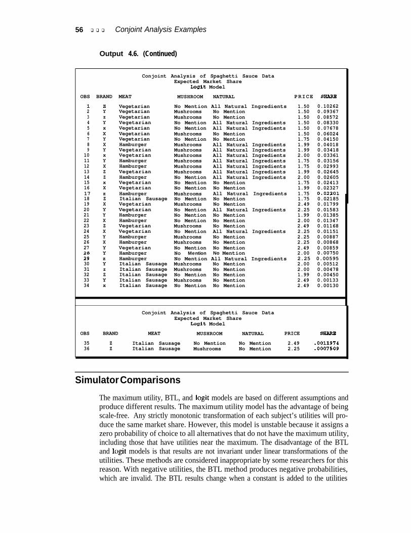
56 q q q Conjoint Analysis Examples
Output 4.6. (Continued)
Conjoint Analysis of Spaghetti Sauce DataExpected Market Share
Logit Model
OBS BRAND MEAT MUSHROOM NATURAL PRICE SHARE
1z Vegetarian No Mention All Natural Ingredients 1.50 0.102622 Y Vegetarian Mushrooms No Mention 1.50 0.093673 z Vegetarian Mushrooms No Mention 1.50 0.085724 Y Vegetarian No Mention All Natural Ingredients 1.50 0.083305 x Vegetarian No Mention All Natural Ingredients 1.50 0.076786 X Vegetarian Mushrooms No Mention 1.50 0.060247 Y Vegetarian No Mention No Mention 1.75 0.041508 X Hamburger Mushrooms All Natural Ingredients 1.99 0.040189 Y Vegetarian Mushrooms All Natural Ingredients 1.99 0.03418
10 x Vegetarian Mushrooms All Natural Ingredients 2.00 0.0336111 Y Hamburger Mushrooms All Natural Ingredients 1.75 0.0315612 X Hamburger Mushrooms All Natural Ingredients 1.75 0.0299313 Z Vegetarian Mushrooms All Natural Ingredients 1.99 0.0264514 Z Hamburger No Mention All Natural Ingredients 2.00 0.0260515 x Vegetarian No Mention No Mention 1.75 0.0241316 X Vegetarian No Mention No Mention 1.99 0.0232717 z Hamburger Mushrooms All Natural Ingredients 1.75 0.022Ol18 Z Italian Sausage No Mention No Mention 1.75 0.0218519 X Vegetarian Mushrooms No Mention 2.49 0.0179920 Y Vegetarian No Mention All Natural Ingredients 2.25 0.0158321 Y Hamburger No Mention No Mention 1.99 0.0138522 X Hamburger No Mention No Mention 2.00 0.0134723 Z Vegetarian Mushrooms No Mention 2.49 0.0116824 X Vegetarian No Mention All Natural Ingredients 2.25 0.0115125 Y Hamburger Mushrooms No Mention 2.25 0.0088726 X Hamburger Mushrooms No Mention 2.25 0.0086827 Y Vegetarian No Mention No Mention 2.49 0.00859
Yii z
Hamburger No Mention No Mention 2.00 0.00750Hamburger No Mention All Natural Ingredients 2.25 0.00595
30 Y Italian Sausage Mushrooms No Mention 2.00 0.0051231 z Italian Sausage Mushrooms No Mention 2.00 0.0047832 Z Italian Sausage No Mention No Mention 1.99 0.0045033 Y Italian Sausage Mushrooms No Mention 2.49 0.0013334 x Italian Sausage No Mention No Mention 2.49 0.00130
Conjoint Analysis of Spaghetti Sauce DataExpected Market Share
Logit Model
OBS BRAND MEAT MUSHROOM NATURAL PRICE SHARE
35 Z Italian Sausage No Mention No Mention 2.49 .001197436 Z Italian Sausage Mushrooms No Mention 2.25 .0007509
Simulator Comparisons
The maximum utility, BTL, and logit models are based on different assumptions andproduce different results. The maximum utility model has the advantage of beingscale-free. Any strictly monotonic transformation of each subject’s utilities will pro-duce the same market share. However, this model is unstable because it assigns azero probability of choice to all alternatives that do not have the maximum utility,including those that have utilities near the maximum. The disadvantage of the BTLand logit models is that results are not invariant under linear transformations of theutilities. These methods are considered inappropriate by some researchers for thisreason. With negative utilities, the BTL method produces negative probabilities,which are invalid. The BTL results change when a constant is added to the utilities
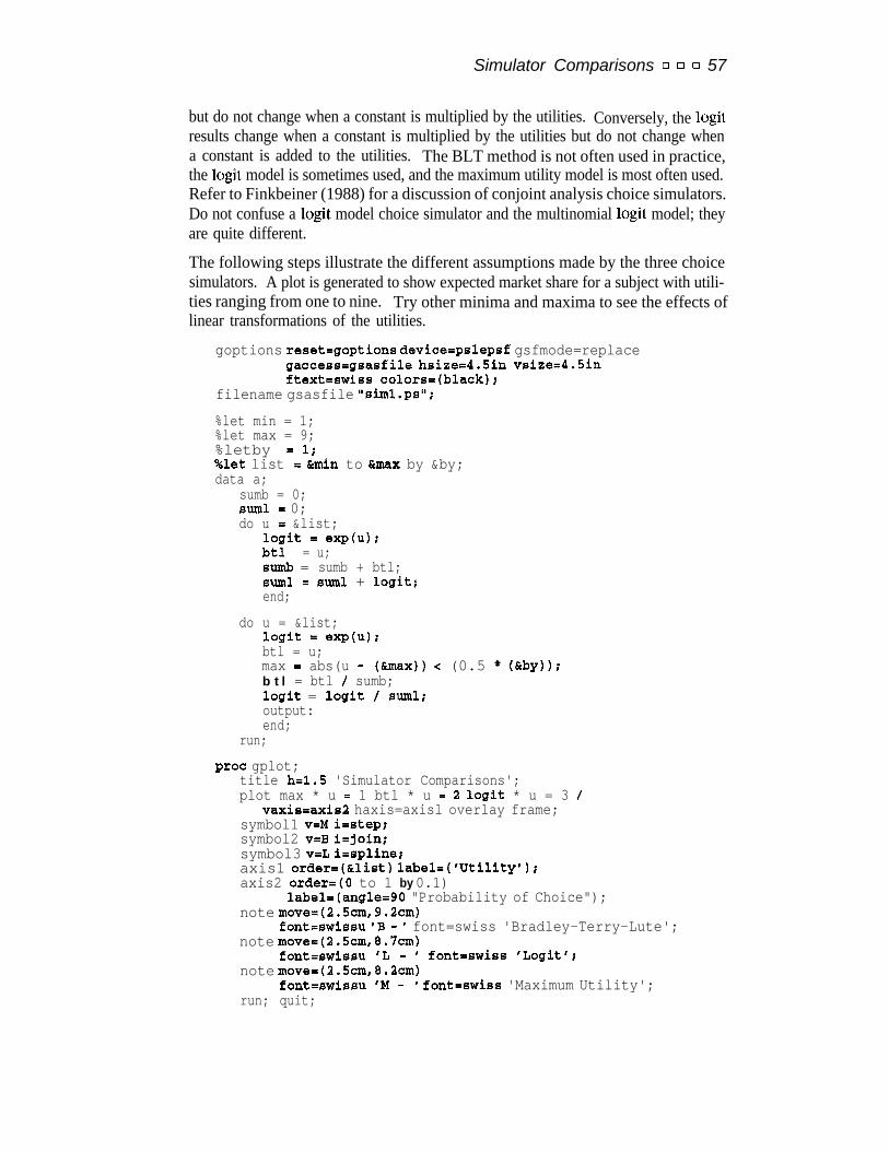
Simulator Comparisons 0 0 0 57
but do not change when a constant is multiplied by the utilities. Conversely, the logitresults change when a constant is multiplied by the utilities but do not change whena constant is added to the utilities. The BLT method is not often used in practice,the logit model is sometimes used, and the maximum utility model is most often used.Refer to Finkbeiner (1988) for a discussion of conjoint analysis choice simulators.Do not confuse a logit model choice simulator and the multinomial logit model; theyare quite different.
The following steps illustrate the different assumptions made by the three choicesimulators. A plot is generated to show expected market share for a subject with utili-ties ranging from one to nine. Try other minima and maxima to see the effects oflinear transformations of the utilities.
goptions reset=goptions devicezpslepsf gsfmode=replacegaccess=gsasfile hsize4.5in vsize=4.5inftext=swies colors=(black);
filename gsasfile "aiml.ps";
%let min = 1;%let max = 9;%letby =l;%let list = &min to &nax by &by;data a;
sumb = 0;suml= 0;do u =I &list;
logit = exp(u);btl = u;surnb = sumb + btl;SUml = sum1 + logit;end;
do u = &list;logit = exp(u);btl = u;max = abs(u - (&max)) < (0.5 * (&by));b t l = btl / sumb;logit = logit / suml;output:end;
run;
proc gplot;title h=1.5 'Simulator Comparisons';plot max * u = 1 btl * u = 2 logit * u = 3 /
vaxis=axis2 haxis=axisl overlay frame;symbol1 v=M i=step;symbol2 v=B i=join;symbol3 v=L i=epline;axis1 order=(&list) label=('Utility');axis2 order=(O to 1 by 0.1)
label=(angle=gO "Probability of Choice");note move=(2.5cm,9.2cm)
font=swissu 'B - I font=swiss 'Bradley-Terry-Lute';note move=(2.5cm,8.7cm)
font=swissu IL - ' font-Swiss 'Logit';note move=(2.5cm,8.2cm)
font=swissu 'M - I font=swiss 'Maximum Utility';run; quit;
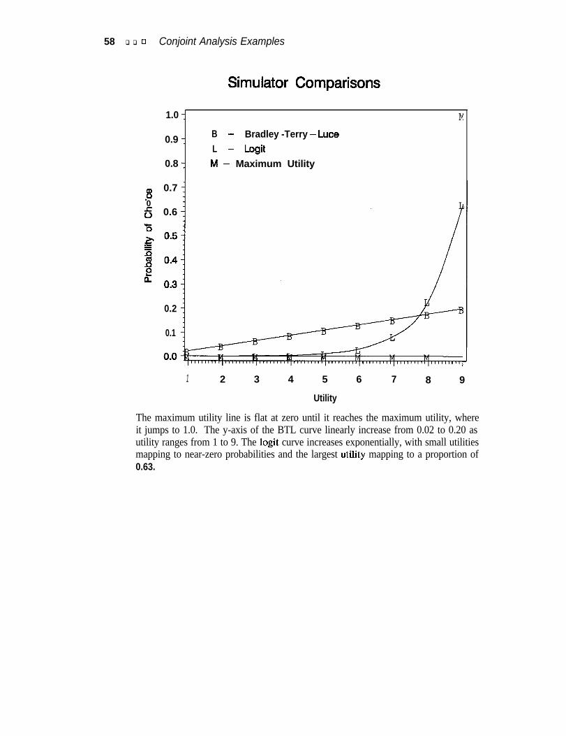
58 q q o Conjoint Analysis Examples
Simulator Comparisons
1.0 :
0.9 :
0.8 :
B - Bradley -Terry - LuteL - LogitM - Maximum Utility
$ 0.7. -05 0.6
0.2
0.1
1 2 3 4 5 6 7 8 9
Utility
The maximum utility line is flat at zero until it reaches the maximum utility, whereit jumps to 1.0. The y-axis of the BTL curve linearly increase from 0.02 to 0.20 asutility ranges from 1 to 9. The logit curve increases exponentially, with small utilitiesmapping to near-zero probabilities and the largest utility mapping to a proportion of0.63.
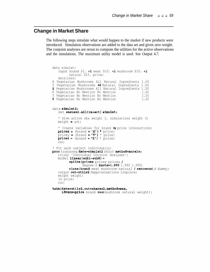
Change in Market Share q q q 59
Change in Market Share
The following steps simulate what would happen to the market if new products wereintroduced. Simulation observations are added to the data set and given zero weight.The conjoint analyses are rerun to compute the utilities for the active observationsand the simulations. The maximum utility model is used. See Output 4.7.
data simulat;input brand $1. tl meat $10. tl mushroom $10. tl
natural $23. price;datalines;
X Vegetarian Mushrooms All Natural Ingredients 1.50Y Vegetarian Mushrooms All Natural Ingredients 1.502 Vegetarian Mushrooms All Natural Ingredients 1.50X Vegetarian No Mention No Mention 1.50Y Vegetarian No Mention No Mention 1.502 Vegetarian No Mention No Mention 1.50
data simulat2;set sasuser.all(in=act) simulat;
* Give active obs weight 1, simulations weight 0;weight = act;
* Create variables for brand by price interactions;pricex = (brand = 'X') * price;pricey = (brand = 'Y') * price;price2 = (brand = 'Z') * price;run;
* Fit each subject individually;proc transreg data=simulat2 short method=morals;
title2 'Individual Conjoint Analyses';model linear(subl-sub8) =
spline(pricex pricey prices /degree-2 knotsz1.995 1.995 1.995)
class(brand meat mushroom natural / zero=sum) / dummy;output out-utils2 dapproximations ireplace;weight weight;id price:run;
%sim(data=utils2,out=shares2,method=max,idvarslprice brand meat mushroom natural weight);
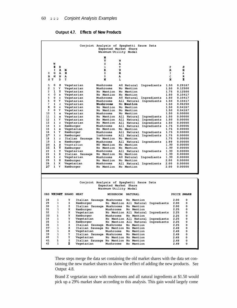
60 q q q Conjoint Analysis Examples
Output 4.7. Effects of New Products
WE BI R
0 0 AB H NS T D
1oz2 1 Y3 1Y4 0 z5 0 x6 0 Y7 1 z8 0 x9 0 Y
10 1 x11 1 x12 1 Y13 1 z14 1 x15 1 x16 1 Y11 1 z18 1 z19 1 x
ii : ii22 1 Y23 1 Z24 1 z25 1 X26 1 X21 1 Y
Conjoint Analysis of Spaghetti Sauce DataExpected Market ShareMaximum Utility Model
Mu NS AIi T
M R wE 0 RA 0 AT M L
Vegetarian Mushrooms All Natural IngredientsVegetarian Mushrooms No MentionVegetarian No Mention No MentionVegetarian No Mention No MentionVegetarian Mushrooms All Natural IngredientsVegetarian Mushrooms All Natural IngredientsVegetarian Wshrooms No YentionVegetarian No Mention No MentionVegetarian No Mention No MentionVegetarian Mushrooms No MentionVegetarian No Mention All Natural IngredientsVegetarian No Mention All Natural IngredientsVegetarian No Mention All Natural IngredientsHamburger Mushrooms All Natural IngredientsVegetarian No Mention No MentionHamburger Mushrooms All Natural IngredientsHamburger lushrooms All Natural IngredientsItalian Sausage No Mention No MentionHamburger Mushrooms All Natural IngredientsVegetarian NO Mention No MentionHamburger No Mention No MentionVegetarian Mushrooms All Natural IngredientsItalian Sausage No Mention No MentionVegetarian Mushrooms All Natural IngredientsHamburger No Mention No MentionVegetarian Mushrooms All Natural IngredientsHamburger No Mention No Mention
PRICE
1.501.501.751.501.501.501.501.501.501.501.501.501.501.751.751.751.751.751.991.991.991.991.991.992.002.002.00
SHARE
0.291670.125000.125000.104170.104170.104170.062500.041670.041670.000000.000000.000000.000000.000060.000000.000000.000000.000000.000000.000000.000000.000000.000000.000000.000000.000000.00000
OBS WRIQHT
28 129 130 131 132 133 134 135 136 131 138 139 140 141 142 1
Conjoint Analysis of Spaghetti Sauce DataExpected Market ShareMaximum Utility Model
BRAND MEAT MUSHROOM NATURAL
Y Italian Sausage Mushrooms No MentionZ Hamburger No Mention All Natural IngredientsZ Italian Sausage Mushrooms No MentionX Hamburger Mushrooms No MentionX Vegetarian No Mention All Natural IngredientsY Hamburger Mushrooms No MentionY Vegetarian No Mention All Natural IngredientsZ Hamburger No Mention All Natural IngredientsZ Italian Sausage Mushrooms No MentionX Italian Sausage No Mention No MentionX Vegetarian Mushrooms No MentionY Italian Sausage Mushrooms No MentionY Vegetarian No Mention No MentionZ Italian Sausage No Mention No Mention2 Vegetarian Mushrooms No Mention
PRICE SHARE
2.00 02.00 02.00 02.25 02.25 02.25 02.25 02.25 02.25 02.49 02.49 02.49 02.49 02.49 02.49 0
These steps merge the data set containing the old market shares with the data set con-taining the new market shares to show the effect of adding the new products. SeeOutput 4.8.
Brand Z vegetarian sauce with mushrooms and all natural ingredients at $1.50 wouldpick up a 29% market share according to this analysis. This gain would largely come
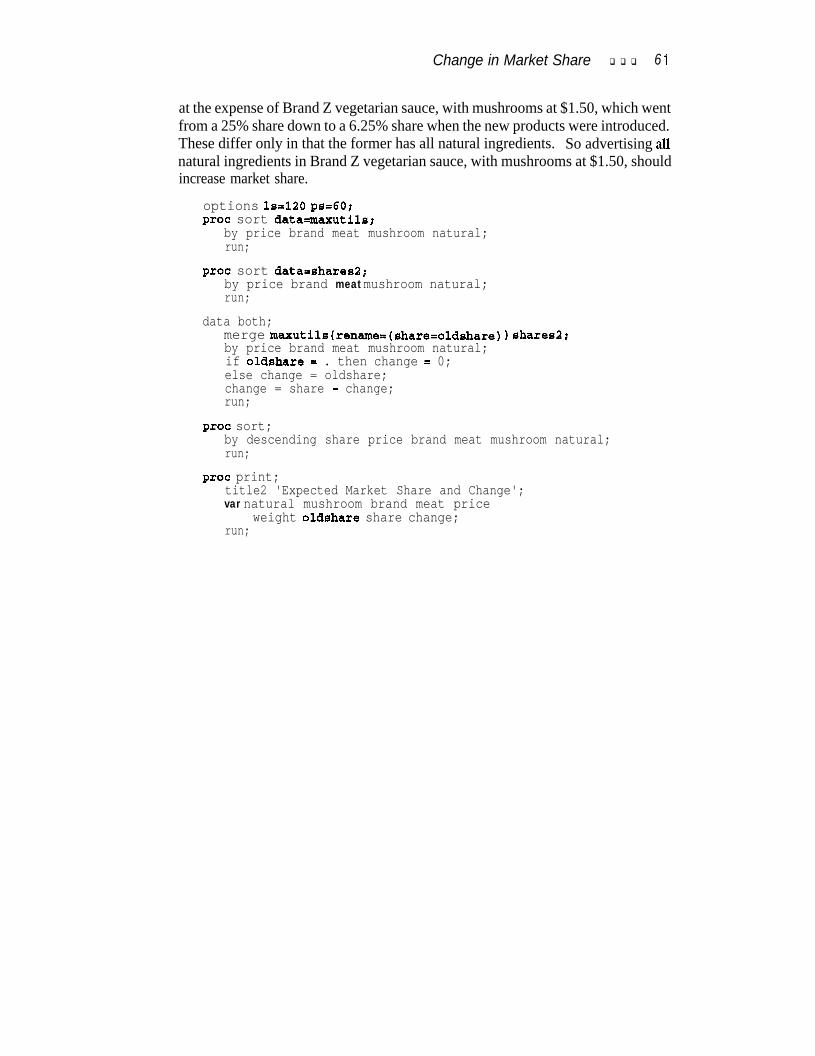
Change in Market Share q q q 6 1
at the expense of Brand Z vegetarian sauce, with mushrooms at $1.50, which wentfrom a 25% share down to a 6.25% share when the new products were introduced.These differ only in that the former has all natural ingredients. So advertising allnatural ingredients in Brand Z vegetarian sauce, with mushrooms at $1.50, shouldincrease market share.
options ls=120 ps=60;proc sort dataqnaxutils;
by price brand meat mushroom natural;run;
proc sort data-shares2;by price brand meat mushroom natural;run;
data both;merge maxutils(rename=(share=oldshare) 1 shares2;by price brand meat mushroom natural;if oldshare = . then change = 0;else change = oldshare;change = share - change;run;
proc sort;by descending share price brand meat mushroom natural;run;
proc print;title2 'Expected Market Share and Change';var natural mushroom brand meat price
weight oldshare share change;run;
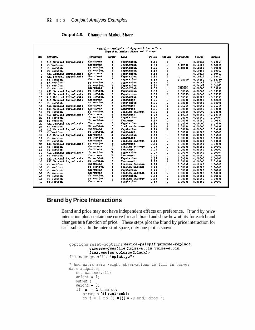
6 2 q q q Conjoint Analysis Examples
Output 4.8. Change in Market Share
OBS NATURAL123456I
;1011121314151617181920212223242526272829303132
All Natural In&ienteNo MentionAll Natural IngredientsNo MentionNo MentionAll Natural IngredientsNo MentionAll Natural IngredientsNo YentionAll Natural IngredientsNo MentionNo MentionAll Natural IngredientlNo MentionNo MentionAll Natural IngredientsNO MentionAll Natural IngredientsAll Natural IngredientsNo MentionNo MentionNo MentionNo MentionNo MentionNo MentionNo Mention
33343536373839404142
All Natural IngredientSNo MentionNo MentionNo MentionAll Natural IngrdientsAll Natural IngrsdisntSNo MantionNo MentionNo MentionNo MentionAll Natural IngredientSAll Natural IngredientaAll Natural IngredientsAll Natural IngrsdisntsNo MentionAll Natural Inaredients
Conjoint Analysis of Spaghetti Sauce DataExpectad Xarket Sham and Change
MUSHROOM BRAND MBAT PRICE WRIQWMwhrooms z Vegetarian 1.50 0Mlrhrooms Y Vegetarian 1.50 1No Mention Y Vegetarian 1.75 1No Mention 2 Vegetarian 1.50 0Mushrooms X Vegetarian 1.50 0Mushroom# Y Vegatarian 1.50 0Mushrooms z Vegetarian 1.50 1NO Mention X Vegetarian 1.50No Mention Y Vegetarian 1.50 iMushroomr X Vegetarian 1.50 1No Mention X Vegetarian 1.50 1No Mention Y Vegetarian 1.50 1No Mention 2 Vegetarian 1.50 1Mushrooms X Hamburger 1.75 1No Mention X Vegetarian 1.75 1Mushrooms Y HsJnhurgor 1.75 1Mushrooms 2 Hamhurgsr 1.75 1No Mention z Italian Sausage 1.75 1Mwhrooms X Hamburger 1.99 1No Mention X Vsgdarian 1.99 1No Mention Y namhurg*r 1.99 1Mushrooms Y Wgetarian 1.99 1No Mention 2 Italian Sausage 1.99 1Mushrooms 2 Vegatarian 1.99 1No lbntion X Hamburger 2.00 1Mushrooms X Vegetarian 2.00 1No Mention Y Hsmhurgsr 2.00 1Mushroomr Y Italian Sausage 2.00 1No Mention Z Hamburger 2.00 1Mushrooms Z Italian Sausage 2.00 1Mushrooms X Hamburger 2.25 1No Mention X Vegetarian 2.25 1Mushrooms Y Hamburger 2.25 1No Mention Y Vegetarian 2.25 1No Mention Z Hamhurgsr 2.25 1Muehrooms Z Italian Sawage 2.25 1No Mention X Italian Sausage 2.49 1Mushrooms X Vegetarian 2.49 1Mushrooms Y Italian Sausage 2.49 1No Mention Y Vegetarian 2.49 1No Mention 2 Italian Sausage 2.49 1Mushrooms 2 Vegetarian 2.49 1
OIDSHARE SHARE CHANGE.
0.125000.12500
0.291670.125000.125000.104170.104170.104170.062500.041670.041670.000000.000000.000000.000000.000000.000000.000000.000000.000000.000000.000000.000000.000000.000000.000000.000000.000000.000000.000000.000000.000000.000000.000000.000000.00000
0.291670.000000.000000.104170.104170.10417
0:25000
o:ooooo0.083330.083330.083330.000000.000000.062500.000000.000000.187500.000000.000000.000000.000000.000000.000000.000000.000000.000000.000000.000000.000000.000000.000000.000000.000000.000000.000000.000000.000000.000000.000000.00000
-0.187500.041670.041670.00000
-0.09333-0.06333-0.083330.000000.00000
-0.062500.000000.00000
-0.187500.000000.000000.000000.000000.000000.000000.000000.000000.000000.000000.000000.000000.000000.000000.000000.000000.000000.000000.000000.000000.000000.000000.00000
0.000000.000000.000000.000000.000000.000000.000000.00000
Brand by Price Interactions
Brand and price may not have independent effects on preference. Brand by priceinteraction plots contain one curve for each brand and show how utility for each brandchanges as a function of price. These steps plot the brand by price interaction foreach subject. In the interest of space, only one plot is shown.
goptions reset=goptions device=pslepsf gsfmode=replacegaccess=gsasfile hsize4.5in vsize4.5inftext=swiss colors=(black);
filename gsasfile “bpint.ps”;
* Add extra zero weight observations to fill in curve;data addprice;
set sasuser.all;weight = 1;output ;weight = 0;if -n- = 1 then do:
array s [al subl-sub8;do j = 1 to 8; s[j] = *; end; drop j;
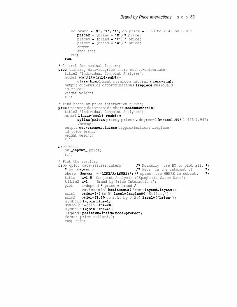
Brand by Price interactions q q q 63
do brand = 'Xl, IY', IZ'; do price = 1.50 to 2.49 by 0.01;pricex = (brand = 'X') * price;pricey = (brand = 'Y') * price;pricez = (brand = '2') * price;output;end; end;
end;runr
* Control for nominal factors;proc transreg data=addprice short method=univariate;
title2 'Individual Conjoint Analyses';model identitytsubl-sub8) =
classtbrand meat mushroom natural / zero=surn);output out=resids dapproximations ireplace residuals;id price:;weight weight;run;
* Find brand by price interaction curves;proc transreg data=resids short method=morals;
title2 'Individual Conjoint Analyses';model lineartrsubl-rsub8) =
spline(pricex pricey pricez / degree=2 knots=1.995 1.995 1.995)/dummy;
output out=sasuser.inters dapproximations ireplace;id price brand;weight weight;run;
proc sort:by -depvar- price;run;
* Plot the results;proc gplot data=sasuser.inters; /* Normally, use BY to plot all. */
* by -depvar-; /* Here, in the interest of */where -depvar- = 'LINEAR(RSUB1)'; /* space, use WHERE to subset. */title h=1.5 'Conjoint Analysis of Spaghetti Sauce Data';title2 h=l 'Brand by Price Interactions';plot a-depend * price = brand /
vaxis=axisl haxis=axis2 frame legendrlegendl;axis1 order=(-5 to 5) label=(angle=90 'Utility');axis2 order=(1.50 to 2.50 by 0.25) label=('Price');symbol1 i=join line&;symbol2 i=join line=20;symbol3 i=join line=ll;legend1 position=inside mode=protect;format price dollar5.2;run; quit;
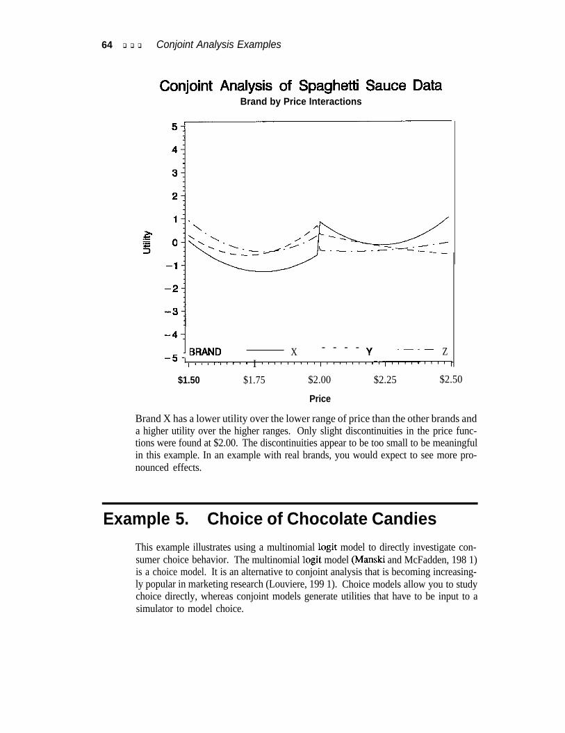
64 q q q Conjoint Analysis Examples
Conjoint Analysis of Spaghetti Sauce DataBrand by Price Interactions
-4:
-5 1 BRAND X - - - - Y _-_- ZII ” ” ” ” I ” “““‘I” 8 “““/““““‘I
$1.50 $1.75 $2.00
Price
$2.25 $2.50
Brand X has a lower utility over the lower range of price than the other brands anda higher utility over the higher ranges. Only slight discontinuities in the price func-tions were found at $2.00. The discontinuities appear to be too small to be meaningfulin this example. In an example with real brands, you would expect to see more pro-nounced effects.
Example 5. Choice of Chocolate CandiesThis example illustrates using a multinomial logit model to directly investigate con-sumer choice behavior. The multinomial logit model (Manski and McFadden, 198 1)is a choice model. It is an alternative to conjoint analysis that is becoming increasing-ly popular in marketing research (Louviere, 199 1). Choice models allow you to studychoice directly, whereas conjoint models generate utilities that have to be input to asimulator to model choice.
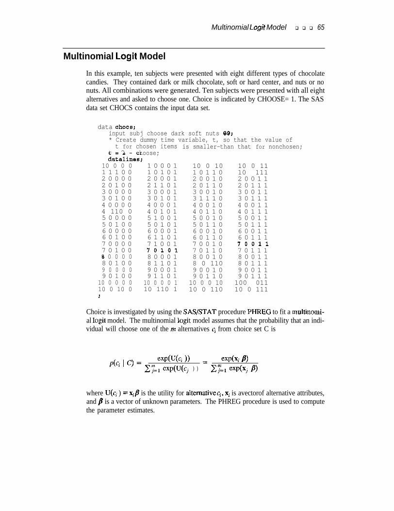
Multinomial Logit Model q q q 65
Multinomial Logit Model
In this example, ten subjects were presented with eight different types of chocolatecandies. They contained dark or milk chocolate, soft or hard center, and nuts or nonuts. All combinations were generated. Ten subjects were presented with all eightalternatives and asked to choose one. Choice is indicated by CHOOSE= 1. The SASdata set CHOCS contains the input data set.
data chocs;input subj choose dark soft nuts @@;* Create dummy time variable, t, so that the value oft for chosen items
t 2 - choose;dat=alines;
10 0 0 01 1 1 0 02 0 0 0 02 0 1 0 03 0 0 0 03 0 1 0 04 0 0 0 04 110 05 0 0 0 05 0 1 0 06 0 0 0 06 0 1 0 07 0 0 0 07 0 1 0 0a 0 0 0 08 0 1 0 09 0 0 0 09 0 1 0 0
10 0 0 0 010 0 10 0;
1 0 0 0 1 10 0 10 10 0 111 0 1 0 1 1 0 1 1 0 10 1112 0 0 0 1 2 0 0 1 0 2 0 0 1 12 1 1 0 1 2 0 1 1 0 2 0 1 1 13 0 0 0 1 3 0 0 1 0 3 0 0 1 13 0 1 0 1 3 1 1 1 0 3 0 1 1 14 0 0 0 1 4 0 0 1 0 4 0 0 1 14 0 1 0 1 4 0 1 1 0 4 0 1 1 15 1 0 0 1 5 0 0 1 0 5 0 0 1 15 0 1 0 1 5 0 1 1 0 5 0 1 1 16 0 0 0 1 6 0 0 1 0 6 0 0 1 16 1 1 0 1 6 0 1 1 0 6 0 1 1 17 1 0 0 1 7 0 0 1 0 7001170101 7 0 1 1 0 7 0 1 1 18 0 0 0 1 8 0 0 1 0 8 0 0 1 18 1 1 0 1 8 0 110 8 0 1 1 19 0 0 0 1 9 0 0 1 0 9 0 0 1 19 1 1 0 1 9 0 1 1 0 9 0 1 1 1
10 0 0 0 1 10 0 0 10 100 01110 110 1 10 0 110 10 0 111
is smaller-than that for nonchosen;
Choice is investigated by using the SAS/STAT procedure PI-IREG to fit a multinomi-al logit model. The multinomial logit model assumes that the probability that an indi-vidual will choose one of the m alternatives ci from choice set C is
expQJ(ci N exdxi B>p(ci ' " = Cy=, eXp(U(Cj )) = x& eXp(Xj p)
where U(ci ) = xi/? is the utility for altemativeci, Xi is avectorof alternative attributes,and /? is a vector of unknown parameters. The PHREG procedure is used to computethe parameter estimates.
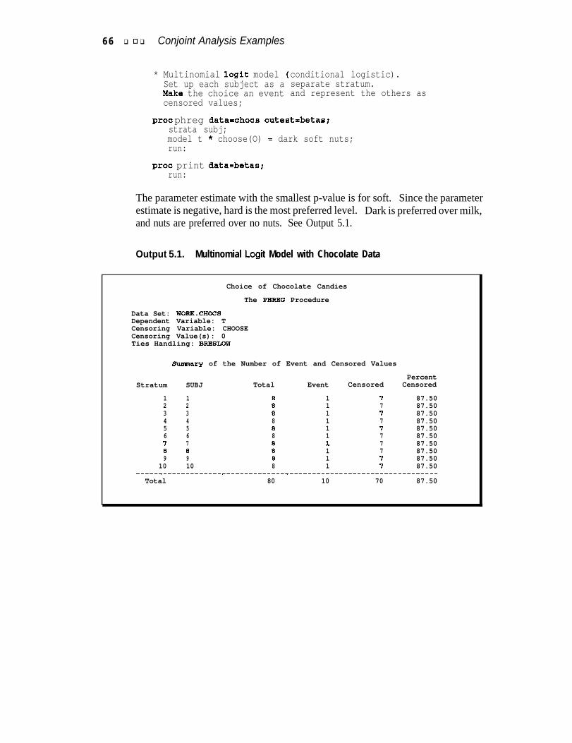
6 6 q cl q Conjoint Analysis Examples
* Multinomial logit model (Set up each subject as aMake the choice an eventcensored values;
conditional logistic).separate stratum.and represent the others as
proc phreg data=chocs outest-betas;strata subj;model t * choose(O) = dark soft nuts;run:
proc print data=betas;run:
The parameter estimate with the smallest p-value is for soft. Since the parameterestimate is negative, hard is the most preferred level. Dark is preferred over milk,and nuts are preferred over no nuts. See Output 5.1.
Output 5.1. Multinomial Logit Model with Chocolate Data
Choice of Chocolate Candies
The PHREG Procedure
Data Set: WOBK.CHoc!SDependent Variable: TCensoring Variable: CHOOSECensoring Value(s): 0Ties Handling: BRESLOW
Sunmary of the Number of Event and Censored Values
PercentStratum SUBJ Total Event Censored Censored
1 1 8 1 I 87.502 2 8 1 7 87.503 3 8 1 I 87.504 4 8 1 7 87.505 5 8 1 I 87.506 6 8 1 7 87.50I 7 8 1 7 87.508 8 8 1 7 87.509 9 8 1 7 87.50
10 10 8 1 I 87.50________________________________________---------------------------
Total 80 10 70 87.50
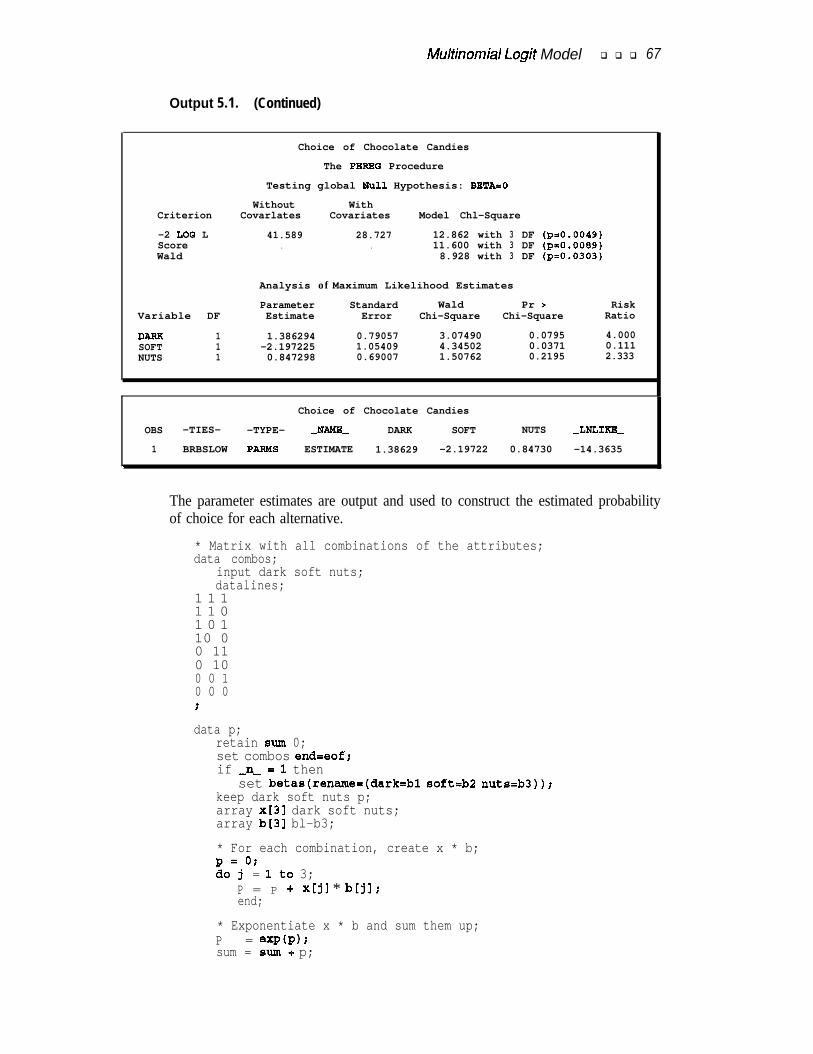
Multinomial Logit Model q q q 67
Output 5.1. (Continued)
Choice of Chocolate Candies
The PHREO Procedure
Testing global Null Hypothesis: BETA=0
Without WithCriterion Covarlates Covariates Model Chl-Square
-2 LOQ L 41.589 28.727 12.862 with 3 DF (p=O.O049)Score . . 11.600 with 3 DF (p=O.O089)Wald 8.928 with 3 DF (p=O.O303)
Analysis of Maximum Likelihood Estimates
Variable DF
DARX 1SOFT 1NUTS 1
Parameter Standard Wald Pr > RiskEstimate Error Chi-Square Chi-Square Ratio
1.386294 0.79057 3.07490 0.0795 4.000-2.197225 1.05409 4.34502 0.0371 0.1110.847298 0.69007 1.50762 0.2195 2.333
Choice of Chocolate Candies
OBS -TIES- -TYPE- -NnMK DARK SOFT NUTS -LNLIKE-
1 BRBSLOW PARMS ESTIMATE 1.38629 -2.19722 0.84730 -14.3635\
The parameter estimates are output and used to construct the estimated probabilityof choice for each alternative.
* Matrix with all combinations of the attributes;data combos;
input dark soft nuts;datalines;
1 1 11 1 01 0 110 00 110 100 0 10 0 0;data p;
retain sum 0;set combos end=eof;if -n- = 1 then
set betas(rename=(dark=bl soft=b2 nuts=b3));keep dark soft nuts p;array x131 dark soft nuts;array b[31 bl-b3;
* For each combination, create x * b;
io=j0;= 1to 3;
P = P + xkil * b[jl;end;
* Exponentiate x * b and sum them up;P = exp(p);sum = sunl+ p;
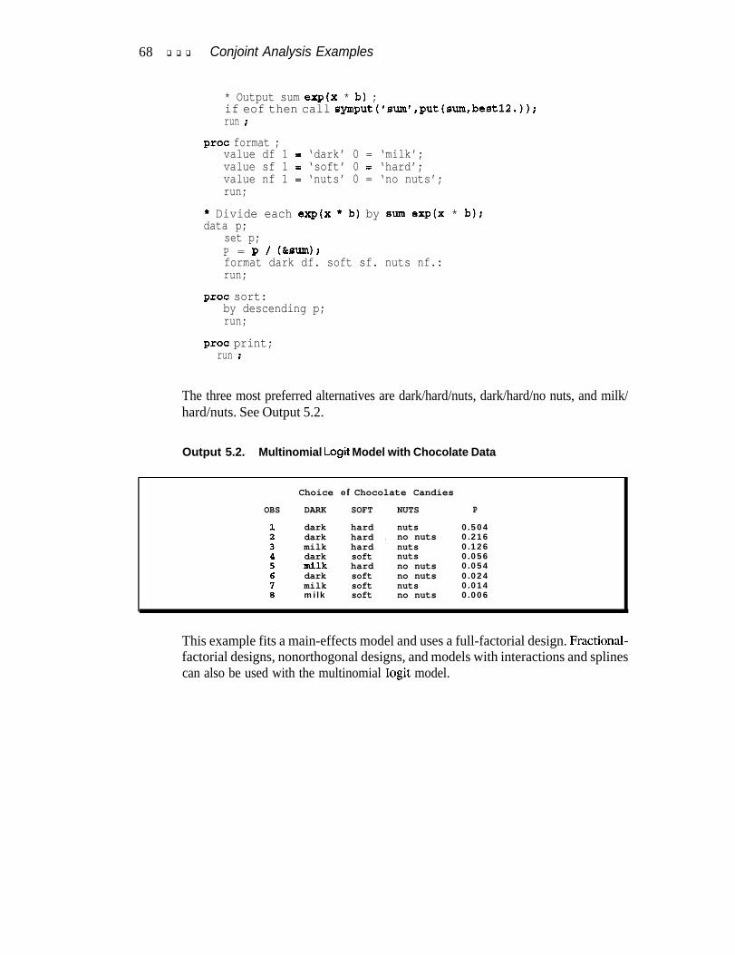
68 q q q Conjoint Analysis Examples
* Output sum exp(x * b) ;if eof then call symput(‘sum’,put(su,bestl2.));run ;
proc format ;value df 1 = ‘dark’ 0 = ‘milk’;value sf 1 = ‘soft’ 0 = ‘hard’;value nf 1 = ‘nuts’ 0 = ‘no nuts’;run;
* Divide each exp(x * b) by sum exp(x * b);data p;
set p;P = p / (&sum);format dark df. soft sf. nuts nf.:run;
proc sort:by descending p;run;
proc print;run i
The three most preferred alternatives are dark/hard/nuts, dark/hard/no nuts, and milk/hard/nuts. See Output 5.2.
Output 5.2. Multinomial Logit Model with Chocolate Data
Choice of Chocolate Candies
OBS DARK SOFT NUTS P
dark harddark hard .milk harddark softmilk harddark softmilk softmilk soft
nutsno nutsnutsnutsno nutsno nutsnutsno nuts
0.5040.2160.1260.0560.0540.0240.0140.006
This example fits a main-effects model and uses a full-factorial design. Fractional-factorial designs, nonorthogonal designs, and models with interactions and splinescan also be used with the multinomial logit model.
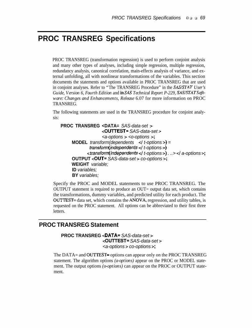
PROC TRANSREG Specifications cl q q 69
PROC TRANSREG Specifications
PROC TRANSREG (transformation regression) is used to perform conjoint analysisand many other types of analyses, including simple regression, multiple regression,redundancy analysis, canonical correlation, main-effects analysis of variance, and ex-ternal unfolding, all with nonlinear transformations of the variables. This sectiondocuments the statements and options available in PROC TRANSREG that are usedin conjoint analyses. Refer to “The TRANSREG Procedure” in the SASISTAT User’sGuide, Version 6, Fourth Edition and inSAS Technical Report P-229, SASISTATSoft-ware: Changes and Enhancements, Release 6.07 for more information on PROCTRANSREG.
The following statements are used in the TRANSREG procedure for conjoint analy-sis:
PROC TRANSREG <DATA= SAS-data-set ><OUTTEST= SAS-data-set ><a-options > <o-options >;
MODEL transform(dependents c/ t-options >) =transform(indejendents -4 t-options >)
<transform(independents 4 t-options >) . ..> 4 a-options >;OUTPUT <OUT= SAS-data-set > co-options >;WEIGHT variable;ID variables;BY variables;
Specify the PROC and MODEL statements to use PROC TRANSREG. TheOUTPUT statement is required to produce an OUT= output data set, which containsthe transformations, dummy variables, and predicted utility for each product. TheOUTTEST= data set, which contains the ANOVA, regression, and utility tables, isrequested on the PROC statement. All options can be abbreviated to their first threeletters.
PROC TRANSREG Statement
PROC TRANSREG <DATA= SAS-data-set ><OUTTEST= SAS-data-set ><a-options > co-options >;
The DATA= and OUTTEST= options can appear only on the PROC TRANSREGstatement. The algorithm options (a-options) appear on the PROC or MODEL state-ment. The output options (o-options) can appear on the PROC or OUTPUT state-ment.
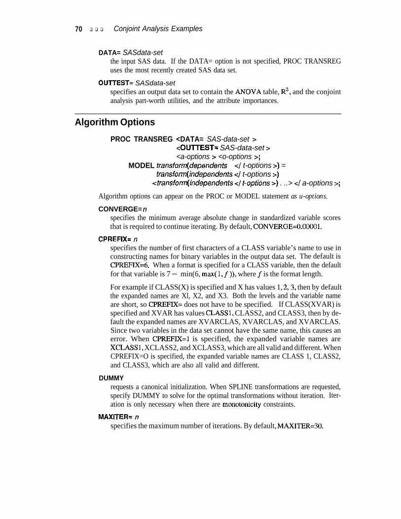
70 q q q Conjoint Analysis Examples
DATA= SASdata-setthe input SAS data. If the DATA= option is not specified, PROC TRANSREGuses the most recently created SAS data set.
OUTTEST= SASdata-setspecifies an output data set to contain the ANOVA table, R2, and the conjointanalysis part-worth utilities, and the attribute importances.
Algorithm Options
PROC TRANSREG <DATA= SAS-data-set ><OUTTEST= SAS-data-set ><a-options > <o-options >;
MODEL transform(dependents </ t-options >) =transform(independents c/ t-options >)
<transform(independents cl t-optidns >) . ..> cl a-options >;
Algorithm options can appear on the PROC or MODEL statement as u-options.CONVERGE= n
specifies the minimum average absolute change in standardized variable scoresthat is required to continue iterating. By default, CONVERGE=O.OOOOl.
CPREFIX= nspecifies the number of first characters of a CLASS variable’s name to use inconstructing names for binary variables in the output data set. The default isCPREFIX=6. When a format is specified for a CLASS variable, then the defaultfor that variable is 7 - min(6, max( 1, f )), where f is the format length.
For example if CLASS(X) is specified and X has values 1, 2,3, then by defaultthe expanded names are Xl, X2, and X3. Both the levels and the variable nameare short, so CPREFIX= does not have to be specified. If CLASS(XVAR) isspecified and XVAR has values CLASSl, CLASS2, and CLASS3, then by de-fault the expanded names are XVARCLAS, XVARCLAS, and XVARCLAS.Since two variables in the data set cannot have the same name, this causes anerror. When CPREFIX=l is specified, the expanded variable names areXCLASSl, XCLASS2, and XCLASS3, which are all valid and different. WhenCPREFIX=O is specified, the expanded variable names are CLASS 1, CLASS2,and CLASS3, which are also all valid and different.
DUMMYrequests a canonical initialization. When SPLINE transformations are requested,specify DUMMY to solve for the optimal transformations without iteration. Iter-ation is only necessary when there are monotonic&y constraints.
MAXITER= nspecifies the maximum number of iterations. By default, MAXITER=30.
Algorithm Options q q q 71
METHOD= MORALSMETHOD= UNIVARIATE
specifies the iterative algorithm. Both METHOD=MORALS andMETHOD=UNIVARIATEfitunivariatemultiple regressionmodels withthepossibility of nonlinear transformations of the variables. They differ in the waythey structure the output data set when there is more than one dependent variable.When it can be used, METHOD=UNIVARIATB is more efficient thanMETHOD=MORALS.
METHOD=UNIVARIATE is used when no transformations of the independentvariables are requested, for example when the independent variables are all desig-nated CLASS, IDENTITY, or PSPLINE. In this case the final set of independentvariables will be the same for all subjects. If transformations such asMONOTONE, LINEAR, SPLINE or MSPLINE are specified for the indepen-dent variables, the transformed independent variables may be different for eachdependent variable and so must be output separately for each dependent variable.In conjoint analysis, there will typically be one dependent variable for each sub-ject. This is illustrated in the examples.
METHOD=UNIVARIATE with more than one dependent variable creates a dataset with the same number of score observations as the original but with more vari-ables. The untransformed dependent variable names are unchanged. The defaulttransformed dependent variable names consist of the prefix T and the originalvariable names. The default dependent variable approximation names consist ofthe prefix A and the original variable names. The full set of independent variablesappears once.
When more than one dependent variable is specified, METHOD=MORALS cre-ates a rolled-out data set with the dependent variable in -DEPEND-, its transfor-mation in T-DEPEND, and its approximation in A-DEPEND. The full set of in-dependents is repeated for each (original) dependent variable.
The procedure chooses a default method based on what is specified on the modelstatement. When transformations of the independent variables are requested, thedefault method is MORALS, Otherwise the default method is UNIVARIATE.
SHORTsuppresses the iteration histories. There are no iterations when there are nomonotonicity constraints, so specifying SHORT eliminates unnecessary output.
TESTprints an overall ANOVA table for each subject. The ANOVA results are, atbest, approximate since the normality and independence assumptions are violat-ed.
UTILITIESprints the part-worth utilities table and an ANOVA table.
72 q q q Conjoint Analysis Examples
Output Options
PROC TRANSREG <DATA= SAS-data-set ><OUlTEST= SAS-data-set ><a-options > co-options >;
OUTPUT <OUT= SAS-data-set > <o-options >;
The OUT= option can only appear on the OUTPUT statement. The other optionscan appear on the PROC or OUTPUT statement as o-options.DAPPROXIMATIONS
includes the approximations to the transformed dependent variables in the outputdata set, which are the predictedutilities for each product. By default, the approx-imation variable name is the original dependent variable name prefixed with anA.
IREPLACEreplaces the original independent variables with the transformed independentvariables in the output data set. The names of the transformed variables in theoutput data set correspond to the names of the original independent variables inthe input data set.
OUT= SASdafa-setnames the output data set. When an OUTPUT statement is specified without theOUT= option, PROC TRANSREG creates a data set and uses the DATAn con-vention. To create a permanent SAS data set, specify a two-level name. Thedata set will contain the original input variables, the dummy variables, the trans-formation of the dependent variable, and the predicted utilities for each product.
RESIDUALSoutputs to the OUT= data set the differences between the observed and predictedutilities. By default, the residual variable name is the original dependent variablename prefixed with an R.
Transformations and Expansions
MODEL transform(dependents c/ t-options >) =transform(independents -4 t-options >)
<transform(independents -4 t-options >) . ..> K/ a-options >;
The following are specified on the MODEL statement as transforms. PSPLINE andCLASS are expansions that create more than one output variable for each input vari-able. The rest are transformations that create one output variable for each input vari-able.
CLASSdesignates variables for analysis as nominal-scale-of-measurement variables.For conjoint analysis the ZERO=SUM t-option is typically specified:CLASS(variables / ZERO=SUM). CLASS expands each variable to a set ofdummy variables. Usually the number output variables for each CLASS variableis the number of different values in the input variables. CLASS should not be
Transformations and Expansions q 0 0 73
specified with the dependent variables.
IDENTITYvariables are not changed by the iterations. IDENTITY(variables) designates in-terval-scale-of-measurement variables when no transformation is permitted.When small data values mean high preference, you will need to use theREFLECT transformation option, Do not use IDENTITY for dependent vari-ables when there are simulation observations, because IDENTITY does not scoremissing values.
LINEARlinearly transforms variables. LINEAR(variabZes) designates interval-scale-of-measurement variables. LINEAR, unlike IDENTITY, allows observations withzero weight to be scored as passive observations. This is useful when some ofthe observations are simulation observations and have missing values in the de-pendentvariable. MissingvaluesareoptimallyscoredinLINEARvariables.When LINEAR is used with dependent variables, a metric conjoint analysis isperformed. When small data values mean high preference, you will need to usethe REFLECT transformation option. LINEAR can also be specified for inde-pendent variables.
LOGITyields logit transformations of variables with values in the interval(0.0 < x < 1.0). LOGIT(variables) specifies the transformation Zog(nc / (1 - x))for each data value X. Unlike other transformations, LOGIT does not have athree-letter abbreviation since LOG means logarithm. LOGIT is typically usedonly for dependent variables.
MONOTONEmonotonically transforms variables; ties are preserved. WhenMONOTONE(variables) is used with dependent variables, a nonmetric conjointanalysis is performed. When small data values mean high preference, you willneed to use the REFLECT transformation option. MONOTONE can also be usedwith independent variables to impose monotonicity on the utilities. When it isknown that monotonicity should exist in an attribute variable, usingMONOTONE instead of CLASS for that attribute may improve prediction. Anoption exists in PROC TRANSREG for optimally untying tied values, but thisoption should not be used because it almost always produces a degenerate result.
MSPLINEmonotonically and smoothly transforms variables. By default,MSPLINE(variables) fits a monotonic quadratic spline with no knots. Knots arespecified as t-options, for example MSPLINE(variubZes / NKNOTS=3) orMSPLINE(vuriubZes / KNOTS=5 TO 15 BY 5). MSPLINE, like MONOTONE,finds amonotonic transformation. Unlike MONOTONE, MSPLINEplaces abound on the df (number of knots + degree) used by the transformation. WithMSPLINE it is possible to allow for nonlinearity in the responses and still haveerror df. This is not always possible with MONOTONE. When small data valuesmean high preference, you will need to use the REFLECT transformation option.MSPLINE can also be used with attribute variables to impose monotonicity onthe utilities.
74 q q q Conjoint Analysis Examples
PSPLINEexpands each variable to apiece-wise polynomial spline basis. By default,PSPLINE(vuriubZes) uses a cubic spline with no knots. Knots are specified ast-options. Specify PSPLINE(variable / DEGREE=2) for an attribute variable toadd a quadratic term to the model. For each PSPLINE variable, d + k output vari-ables are created, where d is the degree of the polynomial and k is the numberof knots. PSPLINE should not be specified with the dependent variables.
RANKperforms a rank transformation, with ranks averaged within ties. Rating-scaledata can be transformed to ranks by specifying RANK(vuriabZes). When smalldata values mean high preference, you will need to use the REFLECT transfor-mation option. RANK is typically used only for dependent variables.
For example if a rating-scale variable has sorted values 1, 1, 1, 2, 3, 3, 4, 5, 5,5, then the rank transformation is 2,2,2,4,5.5,5.5,7,9,9,9. A conjoint analysisof the original rating-scale variable will not usually be the same as a conjoint anal-ysis of a rank transformation of the ratings. With ordinal-scale-of-measurementdata, it is often good to analyze rank transformations instead of the original data.An alternative is to specify MONOTONE, which performs a nonmetric conjointanalysis. For real data, MONOTONE will always produce better fit than RANK,but RANK may lead to better prediction.
SPLINEsmoothly transforms variables. By default, SPLINE(vurZubZes) fits a cubic splinewith no knots. Knots are specified as t-options. Like PSPLINE, SPLINE modelsnonlinearities in the attributes.
Transformation Options
MODEL transform(dependents <I t-options >) =transform(independents <I t-options >)
<transform(independents ~1 t-options S-) . ..> C/ a-options >;
The following are specified on the MODEL statement as t-options’s.DEGREE= n
specifies the degree of the spline. The defaults are DEGREE=3 for SPLINE andPSPLINE, and DEGREE=2 for MSPLINE. For example, to request a quadraticspline, specify SPLINE(vuriubZes / DEGREE=2).
EVENLYis used with the NKNOTS= option to evenly space the knots for splines. Forexample, if SPLINE(X / NKNOTS=2 EVENLY) is specified and X has a mini-mum of 4 and a maximum of 10, then the two interior knots are 6 and 8. WithoutEVENLY, NKNOTS= places knots at percentiles, so the knots are not evenlyspaced.
Transformation Options q •J 0 75
KNOTS= numberlistspecifies the interior knots or break points for splines. By default, there are noknots. For example, to request knots at 1, 2, 3,4, 5, specify SPLINE(variable /KNOTS=1 TO 5).
NKNOTS= kcreates k knots for splines: the first at the lOO/ (k + 1) percentile, the secondat the 200 / (k + 1) percentile, and so on. Knots are always placed at data values;there is no interpolation, For example, with SPLINE(variable / NKNOTS=3),knots are placed at the twenty-fifth percentile, the median, and the seventy-fifthpercentile. By default, NKNOTS=O.
REFLECTreflects the transformation around its mean, Y = -(Y - Y) + Y, after the itera-tions are completed and before the final standardization and results calculations.This option is particularly useful with the dependent variable. When the depen-dent variable consists of ranks with the most preferred combination assigned 1 .O,LINEAR(variable / REFLECT) will reflect the transformation so that positiveutilities mean high preference.
ZERO= SUMconstrains the utilities to sum to zero within each attribute. CLASS(vuriubZes /ZERO=SUM) creates a less than full rank model, but the coefficients are unique-ly determined due to the sum-to-zero constraint.
BY Statement
BY variables;
A BY statement can be used with PROC TRANSREG to obtain separate analyseson observations in groups defined by the BY variables. When a BY statement ap-pears, the procedure expects the input data set to be sorted in order of the BY vari-ables.
If the input data set is not sorted in ascending order, use one of the following alterna-tives:
Use the SORT procedure with a similar BY statement to sort the data.
Use the BY statement options NOTSORTED or DESCENDING in the BYstatement for the TRANSREG procedure. As a cautionary note, theNOTSORTED option does not mean that the data are unsorted. It meansthat the data are arranged in groups (according to values of the BY variables),and these groups are not necessarily in alphabetical or increasing numericorder.
Use the DATASETS procedure (in base SAS software) to create an indexon the BY variables.
For more information on the BY statement, refer to the discussion in SAS Language:Reference, Version 6, First Edition. For more information on the DATASETS proce-dure, refer to the discussion in SAS Procedures Guide, Release 6.06 Edition.
76 q q q Conjoint Analysis Examples
ID Statement
ID variables;
The ID statement includes additional character or numeric variables from the inputdata set in the OUT= data set.
WEIGHT Statement
WEIGHT variable;
A WEIGHT statement can be used in conjoint analysis to distinguish ordinary activeobservations, holdouts, and simulation observations. When a WEIGHT statementis used, a weighted residual sum of squares is minimized. The observation is usedin the analysis only if the value of the WEIGHT statement variable is greater thanzero. For observations with positive weight, the WEIGHT statement has no effecton df or number of observations, but the weights affect most other calculations.
Assigneachactiveobservationaweightof 1. Assigneachholdoutobservationaweight that excludes it from the analysis, such as 0. Assign each simulation observa-tion a different weight that excludes it from the analysis, such as - 1.0. Holdoutsare rated by the subjects and so have nonmissing values in the dependent variables.Simulation observations are not rated and so have missing values in the dependentvariable. It is useful to create a format for the WEIGHT variable that distinguishesthe three types of observations in the input and output data sets.
proc format;value wf 1 = 'Actives
0 = 'Holdout'-1 = 'Simulation';
run:
PROC TRANSREG does not distinguish between weights of zero and - 1.0. Bothweights are nonpositive and exclude the observations from the analysis. The holdoutand simulation observations are given different nonpositive values and a format tomake them easy to distinguish in subsequent analyses and listings. The utilities foreach attribute are computed using only those observations with positive weight. Thepredicted utility is computed for all products, even those with nonpositive weights.
Samples of PROC TRANSREG Usage q q q 77
Samples of PROC TRANSREG UsageConjoint analysis can be performed in many ways with PROC TRANSREG. Thissection provides samples specifications for some typical and more esoteric conjointanalyses. The dependent variable, RATING or RANKING, typically contains ratingsor a ranking of the products. The independent variables, X1-X5, are the attributes.For metric conjoint analysis, the dependent variable is designated LINEAR. For non-metric conjoint analysis, MONOTONE is used. Attributes are usually designated asCLASS variables with the restriction that the utilities within each attribute sum tozero.
The UTILITIES option requests an overall ANOVA table, a table of part-worthutilities, their standard errors, and the importance of each attribute. TheDAPPROXIMATIONS (dependent variable approximations) option outputs to a dataset the predicted utility for each product. The IREPLACE option suppresses the sepa-rate output of transformedindependent variables since the independent variabletransformations are the same as the raw independent variables. The WEIGHT vari-able is used to distinguish active observations from holdouts and simulation observa-tions. The REFLECT transformation option reflects the transformation of the rankingso that large transformed values, positive utility, and positive evaluation will all cor-respond.
Today, metric conjoint analysis is used more often than nomnetric conjoint analysis,and rating-scale data are collected more often than rankings.
Metric Conjoint Analysis with Rank-Order Data
This is a metric conjoint analysis with rank-order data.
proc transreg data=a utilities;model linear(ranking / reflect) = class(xl-x5 / zero=sum);output dapproximations ireplace;weight w;run:
Metric Conjoint Analysis with Rating Scale Data
Here is a typical metric conjoint analysis specification with rating-scale data.
proc transreg data=a utilities:model linear (rating) = class(xl-x5 / zero=sum);output dapproximations ireplace;weight w;run ;
78 q q q Conjoint Analysis Examples
Nonmetric Conjoint Analysis
Next is a nomnetric conjoint analysis specification, which has many parameters forthe transformation.
proc transreg dataea utilities;model monotone(rating) = class(xl-x5 / zero=sum);output dapproximations ireplace;weight w;run:
Monotone Splines
This is a conjoint analysis that is more restrictive than a nomnetric analysis but lessrestrictive than a metric conjoint analysis. By default, the monotone spline transfor-mation has two parameters (degree two with no knots).
proc transreg data=a utilities;model mspline(rating) = class(xl-x5 / zero=sum);output dapproximations ireplace;weight w;run;
If less smoothness is desired, specify knots. For example:
proc transreg datama utilities;model msplinetrating / nknots=3) 3 class(xl-x5 / zero--sum);output dapproximations ireplace;weight w;run;
Each knot uses an extra df.
Constraints on the Utilities
Here is a metric conjoint analysis specification with linearity constraints imposed onX4 and monotonicity constraints imposed on X5.
proc transreg datama utilities;model linear(rating) = class(xl-x3 / zero=sum)
identity(x4) monotone(x5);output dapproximations ireplace;weight w;run;
Constraints on the Utilities q q q 79
Here is another variation:
proc transreg data=a utilities;model linear(rating) = monotone(xl-x5) mspline(price);output dapproximations ireplace;weight w;run:
A Discontinuous Price Function
The utility of price may not be a continuous function of price. It has been frequentlyfound that utility is discontinuous at round numbers such as $1 .OO, $2.00, $100,$1000, and so on. If PRICE has many values in the data set, say over the range $1.05to $3.95, then a monotone function of price with discontinuities at $2.00 and $3.00can be requested as follows.
proc transreg data=a utilities;model lineartranking / reflect) 3 class(xl-x5 / zero=sum)
mspline(price / knots=2 2 2 3 3 3);output dapproximations ireplace;weight w;run;
The monotone spline is degree two. The order of the spline is one greater than thedegree; in this case the order is three. When the same knot value is specified ordertimes, the transformation is discontinuous at the knot. Refer to Kuhfeld and Garratt(1992) for possible applications of splines to conjoint analysis.
More Than One Subject
Typically data are collected for many individuals and then analyzed individually.Each subject’s ratings are entered as a separate dependent variable. Here is an exam-ple.
proc transreg data=a utilities:model linear(ratel-ratelOO) = class(xl-x5 / zeroesurn);output dapproximations ireplace;weight w;run;
80 q q q Conjoint Analysis Examples
ReferencesCarroll, J.D. (1972), “Individual Differences and Multidimensional Scaling,” in
Shepard, R.N., Romney, A.K., and Nerlove, S.B. (Editors), Multidimension-al Scaling: Theory and Applications in the Behavioral Sciences (Volume l),New York: Seminar Press.
Finkbeiner, C.T. (1988) “Comparison of Conjoint Choice Simulators,” Saw-tooth Software Conference Proceedings.
Gifi, A. (1990), Nonlinear Multivariate Analysis, Chichester UK: Wiley.
Green, P.E., and Rao., V.R. (1971), “Conjoint Measurement for QuantifyingJudgmental Data,” Journal of Marketing Research, f&355-363.
Green, P.E., and Srinivasan, V. (1990), “Conjoint Analysis in Marketing: NewDevelopments with Implications for Research and Practice,” Journal ofMarketing, 54,3- 19.
Green, P.E., and Wind, Y. (1975) “New Way to Measure Consumers’ Judg-ments,” Harvard Business Review, July-August, 107- 117.
Kuhfeld, W.F., and Garratt, M. (1992), “Linear Models and Conjoint Analysiswith Nonlinear Spline Transformations,” Paper presented to the AmericanMarketing Association Advanced Research Techniques Forum, Lake Tahoe,Nevada.
Kuhfeld, W.F., Garratt, M., and Tobias, R.D. (1993), “Nonorthogonal Experi-mental Design Theory with Marketing Research Applications,” Paper pre-sented to the American Marketing Association Advanced Research Tech-niques Forum, Monterey, California.
Louviere, J.J. (1988), Analyzing DecisionMaking, Metric Conjoint Analysis,Sage University Papers, Beverly Hills: Sage.
Louviere, J.J. (1991), “Consumer Choice Models and the Design and Analysisof Choice Experiments,” Tutorial presented to the American Marketing As-sociation Advanced Research Techniques Forum, Beaver Creek, Colorado.
Manski, C.F., and McFadden, D. (1981), Structural Analysis of Discrete Datawith Econometric Applications. Cambridge: MIT Press.
Tobias, R.D. (1992), “Saturated Second-Order Two-Level Designs: An Empiri-cal Approach,” unpublished manuscript.
Wittink, D.R., Krishnamurthi L., and Reibstein D.J. (1989), “The Effect of Dif-ferences in the Number of Attribute Levels in Conjoint Results,” MarketingLetters, 1:2, 113- 123.
Young, F.W. (198 l), “Quantitative Analysis of Qualitative Data,” Psychometri-ka, 46,357-388.
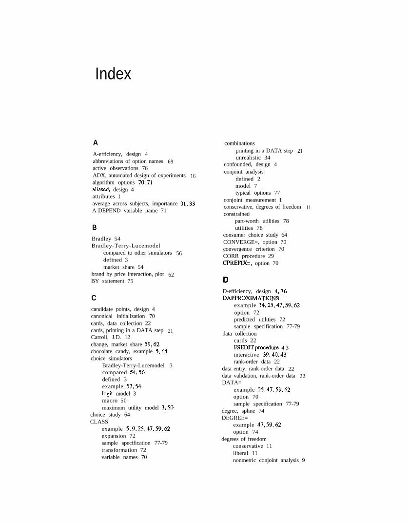
Index
AA-efficiency, design 4abbreviations of option names 69active observations 76ADX, automated design of experiments 16algorithm options 70,71aliased, design 4attributes 1average across subjects, importance 31,33A-DEPEND variable name 71
BBradley 54Bradley-Terry-Lucemodel
compared to other simulators 56defined 3market share 54
brand by price interaction, plot 62BY statement 75
Ccandidate points, design 4canonical initialization 70cards, data collection 22cards, printing in a DATA step 21Carroll, J.D. 12change, market share 59,62chocolate candy, example 5,64choice simulators
Bradley-Terry-Lucemodel 3compared 54,56defined 3example 53,54logit model 3macro 50maximum utility model 3,50
choice study 64CLASS
example 5,9,25,47,59,62expansion 72sample specification 77-79transformation 72variable names 70
combinationsprinting in a DATA step 21unrealistic 34
confounded, design 4conjoint analysis
defined 2model 7typical options 77
conjoint measurement 1conservative, degrees of freedom 11constrained
part-worth utilities 78utilities 78
consumer choice study 64CONVERGE=, option 70convergence criterion 70CORR procedure 29CPREFIX=, option 70
DD-efficiency, design 4,36DAPPROXMATIONS
example 14,25,47,59,62option 72predicted utilities 72sample specification 77-79
data collectioncards 22FSEDITprocedure 4 3interactive 39,40,43rank-order data 22
data entry; rank-order data 22data validation, rank-order data 22DATA=
example 25,47,59,62option 70sample specification 77-79
degree, spline 74DEGREE=
example 47,59,62option 74
degrees of freedomconservative 11liberal 11nonmetric conjoint analysis 9
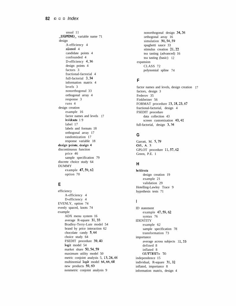
82 0 0 0 Index
usual 11-DEPEND- variable name 71design
A-efficiency 4aliased 4candidate points 4confounded 4D-efficiency 4,36design points 4factors 3fractional-factorial 4full-factorial 3,34information matrix 4levels 3nonorthogonal 33orthogonal array 4response 3runs 4
design creationexample 16factor names and levels 17holdouts 1 9label 17labels and formats 18orthogonal array 17randomization 17response variable 18
design points, design 4discontinuous function
price 46sample specification 79
discrete choice study 64DUMMY
example 47,59,62option 70
Eefficiency
A-efficiency 4D-efficiency 4
EVENLY, option 74evenly spaced, knots 74example
ADX menu system 16average R-square 31,33Bradley-Terry-Lute model 54brand by price interaction 62chocolate candy 5,64choice study 64FSEDIT procedure 39,40logit model 54market share 50,54,59maximum utility model 50metric conjoint analysis 5, 13,24,46multinomial logit model 64,66,68new products 59,60nonmetric conjoint analysis 9
nonorthogonal design 34,36orthogonal array 16simulation 50,54,59spaghetti sauce 33stimulus creation 21,22tea tasting (advanced) 16tea tasting (basic) 12
expansionCLASS 72polynomial spline 74
Ffactor names and levels, design creation 17factors, design 3Federov 35Finkbeiner 56FORMAT procedure 13,18,23,67fractional-factorial, design 4FSEDIT procedure
data collection 43screen customization 40,41
full-factorial, design 3,34
GGarratt, M. 5,79Gifi, A. 3GPLOT procedure 11,57,62Green, P.E. 1
Hholdouts
design creation 19example 21validation 29
Hotelling-Lawley Trace 9hypothesis tests 71
IID statement
example 47,59,62syntax 76
IDENTITYexample 62sample specification 78transformation 73
importanceaverage across subjects 3 1,33defined 8inflated 8OUTTEST= 70
independence 15individual, R-square 31,32inflated, importance 8information matrix, design 4
Index q q q 83
interaction 62interval, variables 73IREPLACE
example 14,25,47,59,62option 72replacing independent variables 72sample specification 77-79
iterationhistory suppressed 71maximum number of 70metric conjoint analysis 6nonmetric conjoint analysis 9
iterative algorithm 71
KKendall Tau 29knots
evenly spaced 74number of 75sample specificationspecifications 75
KNOTS=example 47,59,62option 75
Krishnamurthi, L. 8Kuhfeld, W.F. 5,79
79
Llabel, design creation 17labels and formats, design creation 18levels, design 3liberal, degrees of freedom 11LINEAR
example 5, 14,25,47,59,62sample specification 77-79transformation 73
linear attribute, sample specification 78logit, transformation 73logit model
compared to other simulators 56defined 3market share 54
Louviere, J.J. 1, 64Lute 5 4
MManski, C.F. 64market share
Bradley-Terry-Lucemodel 3,54change 59,62example 50logit model 3,54maximum utility model 3,50simulating 50
maximum number of iterations 70
maximum utility made1compared to other simulators 56defined 3example 50
MAXITER=, option 70McFadden, D. 64METHOD=
MORALS example 25,47,59,62option 71UNIVARIATE example 62
metric conjoint analysisdef ied 2example 5,6,13, 14,24,46iteration 6sample specification 77versus nonmetric 2,77
missing values 73MODEL statement
example 5,9,14,25,47,59,62options 70sample specification 77-79transformation 72transformation options 74
MONOTONEexample 9sample specification 78, 79transformation 73
monotone attribute, sample specification 78monotone spline
sample specification 78,79transformation 73
MORALS algorithm 71more than one subject, sample specification
79MSPLINE
sample specification 78,79transformation 73
multinomial logit model, example 64,66,68multivariate statistics 9
Nnew products, example 59,60NKNOTS=
option 75sample specification 78
naminal, variables 72nonmetric conjoint analysis
defined 2degrees of freedom 9example 9,10iteration 9sample specification 78versus metric 2,77
nonorthogonal, design 33normality 15number of, runs 34
84 q q q Index
0OPTEX procedure 35order, spline 79ordinal, variables 73orthogonal array
design 4design creation 17example 12
OUT=example 25,47,62option 72predicted utilities 72transformation 72
output options 72OUTPUT statement
example 25,47,59,62options 72sample specification 77-79
OUlTEST=example 25importance 70option 70part-worth utilities 70R-square 70used 31utilities 70
Ppart-worth utilities
constrained 78defined 2outputting predicted 72OU’lTEST= 7 0printing 71summing to zero 75
Pearsonr 29perfect fit 15PHREG procedure 65Pillai’s Trace 9PLAN procedure 35plot
brand by price interaction 62transformation 9
polynomial spline, expansion 74predicted utilities
DAPPROX 72OUT= 72variables 27,28
pricediscontinuous function 46sample specification 79
PROC statement 69PSPLINE, transformation 74
RR-square
individual 31,32OUlTEST= 7 0
randomization, design creation 17rank, transformation 74rank-order data
data collection 22dataentry 22data validation 22REFLECT 77sample specification 77versus rating-scale data 77
Rao, V.R. 1rating-scale data
sample specification 77versus rank-order data 77
REFLECTexample 14,25option 75rank-order data 77sample specification 77,79
reflection 14,75Reibstein, D.J. 8replacing independent variables, IREPLACE
72residual variables, RESIDUALS 72RESIDUALS
example 62option 72residual variables 72
response, design 3response variable, design creation 18rolled out data set 71runs
design 4number of 34
Ssample specification
discontinuous function 79linear attribute 78metric conjoint analysis 77monotone attribute 78monotone spline 78,79more than one subject 79nonmetric conjoint analysis 78price 79rank-order data 77rating-scale data 77
screen customization, FSEDIT procedure40,41
SHORTexample 14,25,47,59,62option 71
SIMmacro 5 0
Index q q o 85
simulating, market share 50simulation, example 50simulation observations 23,30,76simulators
Bradley-Terry-Lucemodel 3compared 54,56example 53,54logit model 3macro 50maximum utility model 3,50
spaghetti sauce, example 33specifications 69-76spline
degree 74example 47,59, 62order 79transformation 74
Srinivasan, V. dstimulus creation, DATA step 21summing to zero
part-worth utilities 75utilities 75
Ttea tasting
advanced example 16basic example 12
Terry 54TEST
example 47option 71
tests of hypothesis 71Tobias, R.D. 5trade-offs 1transformation
class 72linear 73logit 7 3monotone 73monotone spline 73none 73options 74,75OUT= 72plot 9rank 74spline 74
TRANSREG procedureadvanced sample 78,79brand by price interaction 62discontinuous price sample 79monotone spline sample 78nonmetric example 9nonmetric sample 78price spline function 47rank data sample 77rating data sample 77simple example 5, 14
simulation 59specifications 69typical example 25typical sample 79
typical options, conjoint analysis 77T-DEPEND variable name 7 1
UUNIVARIATE algorithm 71unrealistic, combinations 34usual, degrees of freedom 11utilities
constrained 78defined 2,7example 5, 14,25option 71outputting predicted 72OUTTEST= 7 0predicted 27,28printing 71sample specification 77-79summing to zero 75
vvalidation, holdouts 29variables
interval 73nominal 72ordinal 73predicted utilities 27replacing in OUT= 72residuals in OUT= 72
WWEIGHT statement
example 25,59,62holdouts 7 6sample specification 77-79
weighted loss function 76Wilks’ Lambda 9Wind, Y. 1Wittink, D.R. 8
YYoung, F.W. 3
ZZERO=
option 75ZERO=SUM example 5,9, 14,25,47,
59,62ZERO=SUM sample specification 77-
79

8 6 q q q Index