Configuration Space Configuration Space ––Basic Path-Planning MethodsBasic Path-Planning Methods

What is a Path?What is a Path?

Tool: Configuration SpaceTool: Configuration Space(C-Space C)(C-Space C)

Configuration Space of a RobotConfiguration Space of a Robot

Space of all its possible configurationsBut the topology of this space is usuallynot that of a Cartesian space

C = S1 x S1

Configuration Space of a RobotConfiguration Space of a Robot

Space of all its possible configurationsBut the topology of this space is usuallynot that of a Cartesian space

C = S1 x S1

Configuration Space of a RobotConfiguration Space of a Robot

Space of all its possible configurationsBut the topology of this space is usuallynot that of a Cartesian space

C = S1 x S1

Structure of Configuration SpaceStructure of Configuration Space

It is a manifoldFor each point q, there is a 1-to-1 mapbetween a neighborhood of q and aCartesian space Rn, where n is thedimension of CThis map is a local coordinate systemcalled a chart.C can always be covered by a finitenumber of charts. Such a set is calledan atlas

ExampleExample

reference point

Case of a Planar Rigid RobotCase of a Planar Rigid Robot

• 3-parameter representation: q = (x,y,θ)with θ ∈ [0,2π). Two charts are needed

• Other representation: q = (x,y,cosθ,sinθ)◊c-space is a 3-D cylinder R2 x S1

embedded in a 4-D space

x

yθ

robotreference direction

workspace

Rigid Robot in 3-D WorkspaceRigid Robot in 3-D Workspace• q = (x,y,z,α,β,γ)

• Other representation: q = (x,y,z,r11,r12,…,r33) where r11,r12, …, r33 are the elements of rotation matrix R: r11 r12 r13 r21 r22 r23 r31 r32 r33with:– ri1

2+ri22+ri3

2 = 1– ri1rj1 + ri2r2j + ri3rj3 = 0– det(R) = +1

The c-space is a 6-D space (manifold) embedded in a 12-D Cartesian space. It is denoted by R3xSO(3)

Parameterization of SO(3)Parameterization of SO(3)• Euler angles: (φ,θ,ψ)

• Unit quaternion: (cos θ/2, n1 sin θ/2, n2 sin θ/2, n3 sin θ/2)

xx

y

zz

xxyy

zz

φφ

x

y

z

θ

xx

yy

zz

ψψ1 ◊ 2 ◊ 3 ◊ 4

Metric in Configuration SpaceMetric in Configuration Space

A metric or distance function d in C is a mapd: (q1,q2) ∈ C2 ◊ d(q1,q2) > 0

such that:– d(q1,q2) = 0 if and only if q1 = q2

– d(q1,q2) = d (q2,q1)– d(q1,q2) < d(q1,q3) + d(q3,q2)

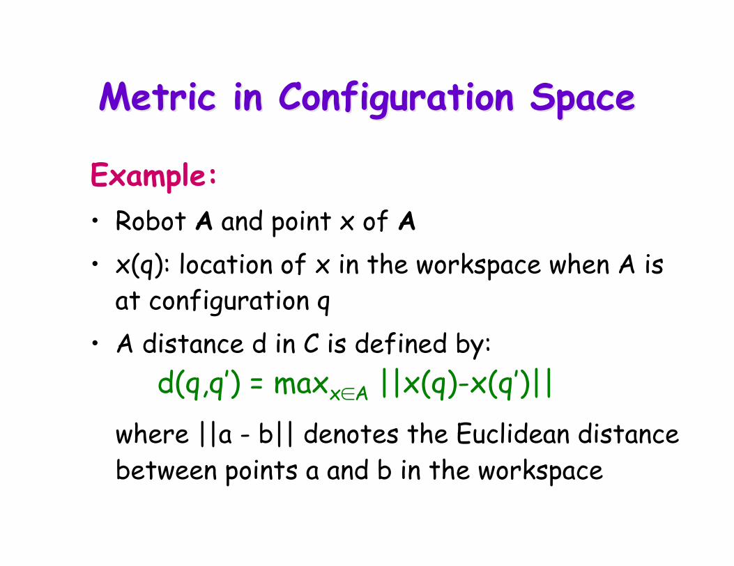
Metric in Configuration SpaceMetric in Configuration Space

Example:• Robot A and point x of A• x(q): location of x in the workspace when A is

at configuration q• A distance d in C is defined by:

d(q,q’) = maxx∈A ||x(q)-x(q’)||where ||a - b|| denotes the Euclidean distancebetween points a and b in the workspace

Notion of a PathNotion of a Path

♣A path in C is a piece of continuous curveconnecting two configurations q and q’:

τ : s ∈ [0,1] ◊ τ (s) ∈ C♣ s’ → s ⇒ d(τ(s),τ(s’)) → 0

q1

q3

q0

qn

q4

q2

τ(s)

Other Possible Constraints on PathOther Possible Constraints on Path

♣ Finite length, smoothness, curvature, etc…♣A trajectory is a path parameterized by time:

τ : t ∈ [0,T] ◊ τ (t) ∈ C

q1

q3

q0

qn

q4

q2

τ(s)

Obstacles in C-SpaceObstacles in C-Space

A configuration q is collision-free, or free, ifthe robot placed at q has null intersection withthe obstacles in the workspaceThe free space F is the set of freeconfigurationsA C-obstacle is the set of configurations wherethe robot collides with a given workspaceobstacleA configuration is semi-free if the robot at thisconfiguration touches obstacles without overlap

Disc Robot in 2-D WorkspaceDisc Robot in 2-D Workspace

Rigid Robot Translating in 2-DRigid Robot Translating in 2-DCB = B A = {b-a | a∈A, b∈B}

a1

b1

b1-a1

Linear-Time Computation ofLinear-Time Computation ofC-Obstacle in 2-DC-Obstacle in 2-D

(convex polygons)

Rigid Robot Translating andRigid Robot Translating andRotating in 2-DRotating in 2-D

C-Obstacle for Articulated RobotC-Obstacle for Articulated Robot

Free and Semi-Free PathsFree and Semi-Free Paths

♣A free path lies entirely in the freespace F

♣A semi-free path lies entirely in thesemi-free space

Remark on Free-Space TopologyRemark on Free-Space Topology• The robot and the obstacles are modeled as closed

subsets, meaning that they contain their boundaries• One can show that the C-obstacles are closed subsets of

the configuration space C as well• Consequently, the free space F is an open subset of C.

Hence, each free configuration is the center of a ball ofnon-zero radius entirely contained in F

• The semi-free space is a closed subset of C. Itsboundary is a superset of the boundary of F

Notion of Notion of Homotopic Homotopic PathsPaths

Two paths with the same endpoints arehomotopic if one can be continuously deformedinto the otherR x S1 example:

τ1 and τ2 are homotopicτ1 and τ3 are not homotopicIn this example, infinity of homotopy classes

q

q’

τ1τ2

τ3

Connectedness of C-SpaceConnectedness of C-Space

C is connected if every two configurations canbe connected by a pathC is simply-connected if any two pathsconnecting the same endpoints are homotopicExamples: R2 or R3

Otherwise C is multiply-connectedExamples: S1 and SO(3) are multiply- connected:- In S1, infinity of homotopy classes- In SO(3), only two homotopy classes

Classes of Classes of Homotopic Homotopic Free PathsFree Paths

Example for Articulated RobotExample for Articulated Robot

Motion-Planning FrameworkMotion-Planning Framework

Continuous representation(configuration space formulation)

Discretization

Graph searching(blind, best-first, A*)

Path-Planning ApproachesPath-Planning Approaches1. Roadmap

Represent the connectivity of the free space by anetwork of 1-D curves

2. Cell decompositionDecompose the free space into simple cells andrepresent the connectivity of the free space by theadjacency graph of these cells

3. Potential fieldDefine a function over the free space that has aglobal minimum at the goal configuration and followits steepest descent

Roadmaps // Retraction

Roadmap methods are also known as retractionmethods.

This is based on the core mathematical relation(usually unstated) that roadmaps are based on aretraction mapping, or projection:

f:Cn :-> R– Each point in Rn maps into some point in the

roadmap.– Each point on the roadmap maps onto itself– The mapping is smooth almost everywhere

dn(f(a),f(b)) < k d(a,b)

Roadmap MethodsRoadmap Methods♣Visibility graphfromIntroduced in theShakey project atSRI in the late 60s.Can produceshortest paths in 2-D configurationspaces

Roadmap MethodsRoadmap Methods♣Visibility graph♣Voronoi diagram

Introduced byComputational Geometryresearchers. Generatepaths that maximizesclearance. Applicablemostly to 2-Dconfiguration spaces

Roadmap MethodsRoadmap Methods♣Visibility graph♣Voronoi diagram♣Silhouette

First complete general method that applies tospaces of any dimension and is singly exponentialin # of dimensions [Canny, 87]

♣Probabilistic roadmaps

Path-Planning ApproachesPath-Planning Approaches1. Roadmap

Represent the connectivity of the freespace by a network of 1-D curves

2. Cell decompositionDecompose the free space into simple cellsand represent the connectivity of the freespace by the adjacency graph of these cells

3. Potential fieldDefine a function over the free space thathas a global minimum at the goalconfiguration and follow its steepestdescent

Cell-Decomposition MethodsCell-Decomposition Methods

Two families of methods:♣Exact cell decomposition

The free space F is represented by acollection of non-overlapping cells whoseunion is exactly FExamples: trapezoidal and cylindricaldecompositions

Trapezoidal decompositionTrapezoidal decomposition

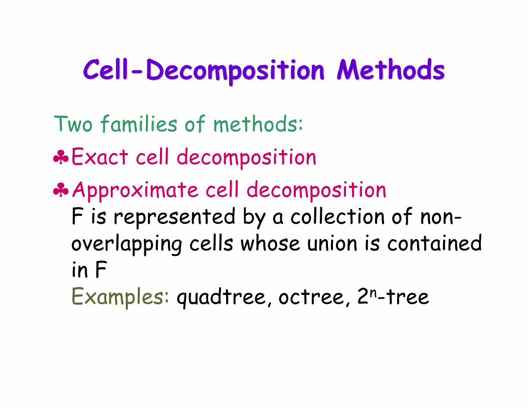
Cell-Decomposition MethodsCell-Decomposition Methods

Two families of methods:♣Exact cell decomposition♣Approximate cell decomposition

F is represented by a collection of non-overlapping cells whose union is containedin FExamples: quadtree, octree, 2n-tree

Octree Octree DecompositionDecomposition

Path-Planning ApproachesPath-Planning Approaches1. Roadmap

Represent the connectivity of the free space by anetwork of 1-D curves

2. Cell decompositionDecompose the free space into simple cells andrepresent the connectivity of the free space by theadjacency graph of these cells

3. Potential fieldDefine a function over the free space that has aglobal minimum at the goal configuration and followits steepest descent

Potential Field MethodsPotential Field Methods

Goal

Goal Force

Obst

acl

e F

orc

e

MotionRobot

)( GoalpGoal xxkF −−=

>

≤∂

∂

−

=

0

020

0

,111

ρρ

ρρρ

ρρρη

if

ifxFObstacle

Goal

Robot

♣Approach initially proposed for real-timecollision avoidance [Khatib, 86]. Hundreds ofpapers published on it.

Path planning: - Regular grid G is placed over C-space- G is searched using a best-first algorithm with potential field as the heuristic function

Potential Field MethodsPotential Field Methods♣Approach initially proposed for real-time

collision avoidance [Khatib, 86]. Hundreds ofpapers published on this topic.

♣ Potential field: Scalar function over the freespace

♣ Ideal field (navigation function): Smooth, globalminimum at the goal, no local minima, grows toinfinity near obstacles

♣ Force applied to robot: Negated gradient ofthe potential field. Always move along thatforce