confidence tubes for multiple quantile …im2131/ps/qqq.pdf · confidence tubes for multiple...

The Annals of Statistics 1999, Vol. 27, No. 4, 1348-1367

CONFIDENCE TUBES FOR MULTIPLE QUANTILE PLOTS VIA EMPIRICAL LIKELIHOOD

BY JOHN H. J. EINMAHL1 AND IAN W. MCKEAGUE

Eindhoven University of Technology and EURANDOM and Florida State University

The nonparametric empirical likelihood approach is used to obtain simultaneous confidence tubes for multiple quantile plots based on k independent (possibly right-censored) samples. These tubes are asymptotically distribution free, except when both k > 3 and censoring is present. Pointwise versions of the confidence tubes, however, are asymptotically distribution free in all cases. The various confidence tubes are valid under minimal conditions. The proposed methods are applied in three real data examples.

1. Introduction. The quantile-quantile (Q-Q) plot is a well known and attractive graphical method for comparing two distributions, especially when confidence limits are added. In this paper we develop Q-Q plot methods for the comparison of two or more distributions from randomly censored data. More specifically, we consider the problem of finding simultaneous confidence tubes for multiple quantile plots (for brevity, multi-Q plots) from k independent samples of possibly right-censored survival times. The multi-Q plot is defined to be the k-dimensional curve (Q1(p),..., Qk(p)) parameterized by 0 <p < 1, where Qj is the quantile function of the jth distribution. It specializes to the ordinary Q-Q plot in the two-sample case.

The comparison of quantile functions is particularly useful for the analysis of survival data in biomedical settings. Frail and strong individuals (corresponding to low and high values of p) often respond to different treatments in different ways, so treatment effects can be hard to determine from comparison of mean or median survival times alone; see, for example, Doksum (1974). The approach developed here allows comparison of treatments simul- taneously across all frailty levels.

Our approach is based on the nonparametric empirical likelihood method. This method was originally developed by Thomas and Grunkemeier (1975) and Owen (1988, 1990) as a way of improving upon Wald-type confidence regions. There now exists a substantial literature on empirical likelihood indicating that it is widely viewed as a desirable and natural approach to

Received May 1998; revised April 1999. 1Supported in part by a Fulbright grant and by European Union Grant ERB CHRX-CT

94-0693. AMS 1991 subject classifications. Primary 62G15; secondary 62G20. Key words and phrases. Censoring, confidence region, distribution-free, k-sample comparison,

nonparametric likelihood ratio, quantile-quantile plot. 1348

CONFIDENCE TUBES FOR QUANTILE PLOTS

statistical inference in a variety of settings. Moreover, there is considerable evidence that procedures based on the method outperform competing procedures. Empirical likelihood based confidence bands for individual quantile functions have recently been derived in Li, Hollander, McKeague and Yang (1996). Naik-Nimbalkar and Rajarshi (1997) employed the approach to test for equality of k medians; their test naturally extends to a test for equality of k quantiles.

We use the nonparametric empirical likelihood approach to derive asymptotic simultaneous confidence tubes for multi-Q plots based on k independent random samples, including confidence bands for ordinary Q-Q plots (k = 2). The tubes are applicable to situations with or without random censoring. The limiting processes involved in the construction of the tubes are distribution free, except when k > 3 and censoring is present. In general, we are able to obtain asymptotically distribution-free pointwise confidence regions for the multi-Q plot. The various confidence tubes are valid under minimal conditions, although for convenience we shall assume continuity of the underlying distribution functions.

Q-Q plots are studied in detail using classical methods in Doksum (1974, 1977), Doksum and Sievers (1976) and Switzer (1976) for models without censoring; see Shorack and Wellner [(1986), pages 652-657] for a summary and discussion. For models with censoring, Wald-type simultaneous confidence bands for Q-Q plots are obtained in Aly (1986), but restrictive differen- tiability conditions on the underlying distribution functions are required. The k-sample problem without censoring is studied in Nair (1978, 1982), but essentially only pairwise comparisons are made there. A review of graphical methods in nonparametric statistics with extensive coverage of Q-Q plots can be found in Fisher (1983). Some refined approximation results for normalized Q-Q plots with statistical applications have been established in Beirlant and Deheuvels (1990) for the uncensored case and Deheuvels and Einmahl (1992) in the censored case.

The paper is organized as follows. The proposed confidence tubes and the main results are presented in Section 2. Our approach is illustrated in Section 3 using three real data examples. All the proofs are contained in Section 4.

2. Main results. We begin by specifying the setup precisely and intro- ducing the basic notation. It is convenient first to recall the notation in the one-sample case. For the corresponding notation in the general k-sample case, we use a further subscript j to refer to the jth sample.

The random censorship model deals with n i.i.d. pairs (Zi, 5i), i = 1,..., n, obtained from two independent random samples Xi and Yi, i = 1,..., n, in the following way: Zi = Xi A Yi, (i = liXi Yi. The distribution functions of Xi and Yi are denoted F and G, respectively, and F is assumed to be continuous. We will work with nonnegative Xi and Yi, but this restriction is in fact not needed anywhere; see the discussion at the end of this section. The (right-continuous) quantile function corresponding to F is denoted by Q. We

1349

J. H. J. EINMAHL AND I. W. MCKEAGUE

write

L(F) = f1 (1F(Zi) - F(Zi -))8i(i - F(Zi))1 i=l (1)

for the likelihood, where F belongs to 0, the space of all distribution functions on [0,oo). The ordered uncensored survival times, that is, the Xi with corresponding 8i = 1, are written 0 T< T . _ TN < oo, and rj = Ein l(zi .>} denotes the size of the risk set at Tj - . The empirical likelihood ratio for F(t) = p (given 0 < p < 1) is defined by

sup{L(F): F(t) =p, P E @

sup{L(F): F E O} Note that the sup in the denominator is attained by the Kaplan-Meier (or product-limit) estimator

n(t) = 1 - - 1- i: Ti<t ri)

It can be shown with the aid of Lagrange's method [see Thomas and Grunke- meier (1975) or Li (1995)] that

-21ogR(t) = -2 (ri- 1)log (1 + ) - riog 1+- , i: Ti<t ri - I ri

where the Lagrange multiplier A > D = maxi Ti < t(1 - ri) satisfies the equation

(2.1) n 1- -P i:Ti <t ri + A)

Now we turn to the multisample setup. The k samples are assumed to be independent with sample sizes denoted n1,..., nk; write n = Ej= nj. Set F = (F1,..., Fk) and define the multi-Q plot to be

{(Q,(P),..., Qk(P)):0 <p < }. Observe that this is the classical Q-Q plot when k = 2. In the sequel we consider the following more convenient version of the multi-Q plot: the graph Q of the function

t1 (Q2(F(tl)),...,Qk(Fl(tl))) for t1 > 0. Denote the joint likelihood by

k

L(F)= nL() j=1

and the empirical likelihood ratio at t = (t1,..., tk) by

sup{L(F): Fj(tj) = F1(tl) for all j 2,...,k,i G ok} R(t) = . .

sup{L(F): F E Ok)

1350

--\ k


Again we find, using Lagrange's method with the k - 1 constraints, Fl(t1) - Fj(tj), j = 2,..., k, that

-2 log R(t)

(2.2) k

C C = -2E (rji - )log +j l -rj og(i + - j= 1 i: Tji < tj Fji -- i ji

where the Aj, j = 2,..., k, satisfy the k - 1 equations

(2.3) ~ i: Tli < t( rli - A1) i: Tji<tj( rji + A ) here we have set A1 = -E-2 Aj (so Lk= Aj = 0) and the Aj should satisfy j > Dj forj= 1,...,k.

Later we show that this system of equations indeed has a unique solution; see Lemma 4.1. In the one-sample case, it is immediately clear that the corresponding Lagrange multiplier equation (2.1) has a unique solution, but it is not obvious in the multisample case. Computation of the Aj's can be carried out using a special-purpose root-finding procedure which exploits the monotonicity of the r.h.s. of (2.3) as a function of Aj (see Section 3 and the proof of Lemma 4.1).

The various confidence sets we propose are easily obtained from the main theorem below and are presented in the three subsequent theorems. These confidence sets are all of the form {t: R(t) > c}, where c is derived using asymptotic considerations.

Before stating our main theorem we introduce some more notation. We assume throughout that nj/n - pj > 0 as n -> co for j = 1,..., k (although with some care this condition can be relaxed to nj - oo). Define

2 s dFj(u) 2s) ( = (1 - Fj(u))(- - G (u -))

We will need the k x k-matrix D = D(t) with entries

ai(t) j(tj) I /-- rij, for j i, v/Pi Pj

dij = dl Oi(ti) a T..i, I -- 7-1i forj = i,

Pi l=i

where l-J A i, 14: jO'j2 ( tt) /PI

1Iij = k 1 2 ( tl) /p! q=lj 1 lq (l)/P

(the empty product is defined to be 1). Also define V = V(t) to be the random k-vector with jth entry Wj(oa2(tj))/oj(tj), where the Wj are independent standard Wiener processes. Let T, be such that Fl(T1) > 0 and let r2 > r1 be

1351


such that F1(72) < 1, G1(T2) < 1 and Gj(Qj(F1(T2))) < 1 for j = 2,..., k. We assume throughout that the Fj are continuous.

THEOREM 2.1. When R, D and V are evaluated at t = (t1, Q2(Fl(tl)),..., Qk(Fl(tl))) for T1 < t1 < T2, we have

(2.4) -2 log R -> I DV l2

on D[ 71, 72], with 1 i the k-dimensional Euclidian norm.

Write the restriction of Q to t1 E [r1, 72] as Q[Tr, 72]. In the next theorem we consider the important case k = 2, in which the multi-Q plot reduces to the usual Q-Q plot. Define c,[sl, s2] for 0 < a < 1 by

P( sup W12(s)/s <C[S S2]) =1- a. S E[ S1, S2]

Set c^ = ca[ (2(Ti), 2(T2)], where

(2.5) _(tl) __ +/ ) n, n, (2.5) 2(t) n{ n(1( t ) ?2 (Q2n2(F11(ti))) }

with

(2.6) : 2 r ( 1

i:'T ,<s rji(ji -i

and with Q2n2 the (right-continuous) quantile function corresponding to F2n2. Now we define the confidence band for Q[T1, 7'2] to be

= {t E [1, 72] x[0,O): -2log R(t) < c}.

THEOREM 2.2. In the censored case, for k = 2 and 0 < a < 1,

lim P(Q[71, 2] e2 ) =1 - a. n - oo

REMARK 2.1. In the uncensored case (and k = 2) we have that

(22(t ) (2())) P1 2 F1(t1 P )

(2.7) - + -- l

= 1 ) 2(t). Pi P2

( -+1

P1 r 11)

1352


Therefore for this case we can replace the a2(tl) defined in (2.5) by the simpler but almost equivalent estimator

I i Flnl(tl) 2(tl) n --n - - ?

n, n2 1 - Fln(tl)

For use in c^,, we can replace (2(tl) by

Flnl( tl) 1 -Flnl(tl)

Observe that this last expression is not an estimator of r2(tl) but of or2(t1). This however makes no difference because of (2.7) and the fact that for c > 0

sup W1(s)/s = sup W (s)/s. sE[sl,s2] s [cs, cs2]

Of course, here the Kaplan-Meier estimator Fln, is just the empirical distribution function of the first sample.

Next we return to general k > 2, but assume that there is no censoring. Note that in this case the assumptions on T2 reduce to F1(T2) < 1. Define CJ[s, s2] for 0 < a < 1 by

k1 -1 (2.8) P sup - E W2(s) <C,s s] =1- a.

sc[sl,s2] $ j=l

Set C, = Ca[ -2(7i), 12(72)], where

^2 \ _ ^Fn(t1) 2(t) 1 - Flnl(tl)

Define the confidence tube for Q[71, T2] by

J= {t E [71,r2] X[,O)k-1: -2log R(t) < ,)}.

THEOREM 2.3. In the absence of censoring, for all k 2 2 and 0 < a < 1,

lim P(Q[T1,T2] E a) = 1 - a. n - oo

Now we allow censoring and k > 2 but take T2 = rl. Set Q[T1] = Q[T1, T1]. Define the confidence region for Q[ 1] by

= {t E {T1} X[O,mo)k : -21og R(t) < X,2

where X2 is the upper a-quantile of the chi-square distribution with k - 1 degrees of freedom. In the case k = 2 note that o amounts to a confidence interval for the Fl(rT)-quantile of F2.

1353


THEOREM 2.4. In the censored case, for all k > 2 and 0 < a < 1,

limP(Q[Tl] EG) = 1 - a. n -> oo

The asymptotic null distribution in the test for equality of k medians developed by Naik-Nimbalkar and Rajarshi (1997) can be essentially derived from the proof of Theorem 2.4 by taking z1 as their estimator 0* of the common median.

Finally we establish an interval property for the confidence tube ~ (which also applies to S and -): one-dimensional cross-sections parallel to a given axis are intervals. This is useful for computing the various confidence sets because points belonging to them can then be found by a simple search strategy that sweeps along each axis.

THEOREM 2.5. Suppose that t() = (t1,...,t( , ) E for 1= 1,2, where t(l) < t(2). Then t* = (t, ..., t ,., t) e for any tj E [t1), t2)].

In the two-sample case (k = 2) we have a somewhat stronger result.

THEOREM 2.6. Let (t0l), t(l)), I = 1, 2, belong to the confidence band M and suppose ) t)(2) t2 and t) t1. Then (t, t?) also belongs to M whenever t2) < tj < tl) and t(1) < t < t(2)

This theorem (as well as Theorem 2.5) implies, by taking tl) = t2) or t2) = t2), that the intersection of the band M with a vertical or horizontal line is an interval. In addition, it shows that the bands are nondecreasing in the sense that their lower or upper boundaries are nondecreasing.

Discussion. We wish to emphasize that our approach, including the defi- nition of the multi-Q plot, is new even in the uncensored case. We also remind that nonnegativity of the observations is not needed anywhere in the proofs. This is especially useful in the uncensored case, where often the k samples do not represent life or failure times or when a transformation is applied to the data (see the third example in Section 3).

Another desirable feature of our approach is that the confidence bands and tubes are essentially invariant under permutations of the order of the k samples involved. (Only at the two "ends" of the tube does the first sample play a somewhat special role.)

We did not formulate a version of our confidence tubes in the censored case for k > 3 since then IIDV112 in (2.4) is not distribution free, even when only one of the k samples is subject to censoring. Our approach can, however, be generalized to this situation by estimating all the unknowns appearing in D and V and then using simulation. This means that we replace D by C (given in the proof of Theorem 2.1), tj by Qjn(Fn(t)) for j = 2,..., k, and oj2 by Cj2. The process to be simulated has the form |lCV112, where V is the estimated version of V. Hence, approximate 1 - a confidence tubes can be

1354


constructed for the censored case as well, but we do not pursue this in further detail here.

The one-sample Q-Q plot, t -> Q(Fo(t)) with Fo known, is essentially treated in Li, Hollander, McKeague and Yang (1996), since their confidence bands for Q(p) can be transformed to bands for Q(Fo(t)) by the time change p = Fo(t). The present paper can be seen as a generalization of their approach to the k-sample case.

For uncensored data, in the two-sample Q-Q plot case, our confidence bands perform well in the tails due to the weighting which naturally arises when using the empirical likelihood method. Our bands share this property with the weighted bands (W bands) introduced in Doksum and Sievers (1976), which are based on the standardized two-sample empirical process. The bands in Switzer (1976) [and Aly (1986) for the censored case] are much wider in the tails, since they are based on the unweighted empirical process. All these procedures as well as our procedures are essentially based on the inversion of a distance between empirical distribution functions (or Kaplan-Meier estimators). In fact, the W bands are asymptotically equivalent to our bands in the uncensored case.

3. Applications to real data. In this section we illustrate our approach in three real data examples.

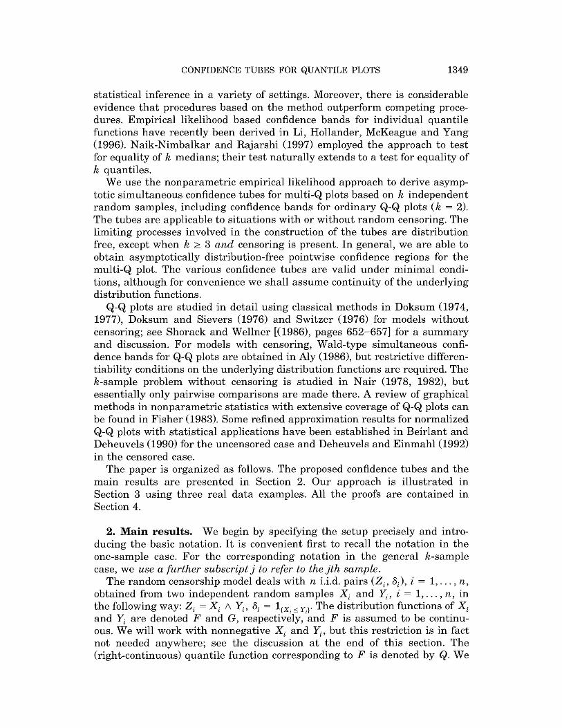
First we consider a biomedical example for the two-sample case with censored survival data. The data come from a Mayo Clinic trial involving a treatment for primary biliary cirrhosis of the liver; see Fleming and Harring- ton (1991) for discussion. A total of n = 312 patients participated in the randomized clinical trial, 158 receiving the treatment (D-penicillamine) and 154 receiving a placebo. Censoring is heavy (187 of the 312 observations are censored). Figure 1 displays the 90% confidence band (and pointwise confidence intervals) for the Q-Q plot of treatment versus placebo for survival time in days. The standard empirical Q-Q plot based on quantiles of the Kaplan-Meier estimator is also displayed. Note that although the diagonal departs from the pointwise confidence region at some points, it remains within the simultaneous band, so there is no overall evidence of a difference between treatment and placebo.

The second example also illustrates the two-sample case. Hollander, McKeague and Yang (1997) analyzed data on 432 manuscripts submitted to the Theory and Methods Section of JASA during 1994. Each observation consists of the number of days between a manuscript's submission and its first review or the end of the year, along with a censoring indicator (1 if a paper received its first review by the end of the year; 0 otherwise). Similar data (on 444 manuscripts) are available for 1995. The censoring is light (330 of the 876 observations are censored) compared with the previous example. It is of interest to look for differences in the pattern of review times for the two years. Figure 2 displays the 95% confidence band (and pointwise confidence intervals) for the Q-Q plot. The lower endpoints of the pointwise confidence intervals touch the diagonal between 10 and 25 days, which might suggest

1355


o

t O I ~~~~'<o1 o ___~~~~~~~r -"J-' , .

2 ? --r o?'? ' F

C0 r1 i .*' r"--

E

' " ?r--'-

o -

0 1000 2000 3000 Placebo (survival in days)

FIG. 1. 90% confidence band (solid line) for the treatment versus placebo Q-Q plot in the Mayo Clinic trial, for 186 < tl < 2976 days; pointwise confidence intervals (short dashed line), empirical Q-Q plot (long dashed line).

that "rapid" reviews were faster in 1994 than in 1995. However, the diagonal is completely contained within the simultaneous band, so there is no overall evidence of a difference between the patterns of review times.

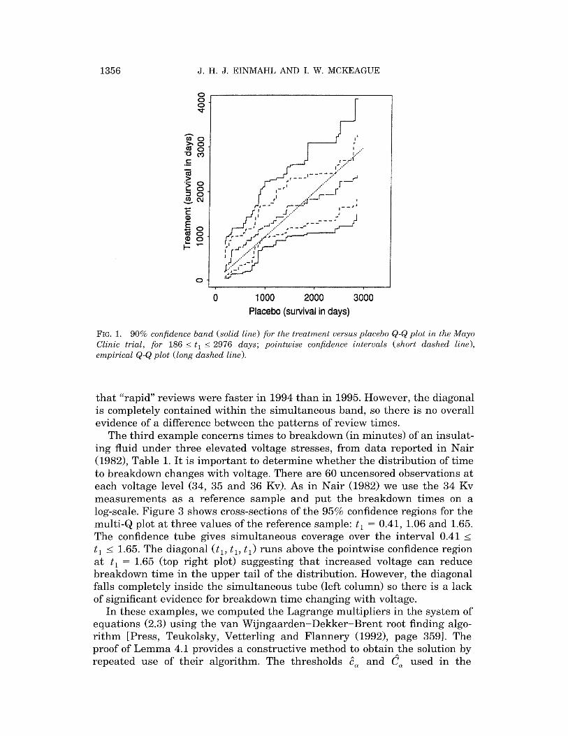
The third example concerns times to breakdown (in minutes) of an insulating fluid under three elevated voltage stresses, from data reported in Nair (1982), Table 1. It is important to determine whether the distribution of time to breakdown changes with voltage. There are 60 uncensored observations at each voltage level (34, 35 and 36 Kv). As in Nair (1982) we use the 34 Kv measurements as a reference sample and put the breakdown times on a log-scale. Figure 3 shows cross-sections of the 95% confidence regions for the multi-Q plot at three values of the reference sample: t1 = 0.41, 1.06 and 1.65. The confidence tube gives simultaneous coverage over the interval 0.41 < t, < 1.65. The diagonal (tl, tl, t,) runs above the pointwise confidence region at t, = 1.65 (top right plot) suggesting that increased voltage can reduce breakdown time in the upper tail of the distribution. However, the diagonal falls completely inside the simultaneous tube (left column) so there is a lack of significant evidence for breakdown time changing with voltage.

In these examples, we computed the Lagrange multipliers in the system of equations (2.3) using the van Wijngaarden-Dekker-Brent root finding algorithm [Press, Teukolsky, Vetterling and Flannery (1992), page 359]. The proof of Lemma 4.1 provides a constructive method to obtain the solution by repeated use of their algorithm. The thresholds c^ and Ca used in the

1356


o

0

o -

o - 'r' 'C

0- 0',1'.

0 50 100 150 200 Days to First Review (1994)

FIG. 2. 95% confidence band (solid line) for the Q-Q plot based on the JASA time-to-first-review data, for 5 < t1 < 195 days; pointwise confidence intervals (short dashed line), empirical Q-Q plot (long dashed line).

confidence bands and tubes were computed by simulation of the Wiener processes on a fine grid.

4. Proofs. Here we present proofs of the theorems in Section 2. Some lemmas used in these proofs are given at the end of this section.

PROOF OF THEOREM 2.1. First we note that, by Lemma 4.1, below the system of equations in (2.3) with A1 replaced by -_ 2 A has a unique solution for all k > 2.

Define gj: (Dj, o) --> R by

gj(A)= i log I

for j = 1,..., k. Denote aj = gj(O) = log Sj(tj), where Sj is the Kaplan-Meier estimator of S= 1 - F and bj = gj(0) = &j2(tj)/nj with A2 as in (2.6). Here tj = Qj(Fl(t)) for j = 2,..., k. Taylor series expansions of g and gj, in conjunction with Lemma 4.2 and the argument of Li [(1995), proof of (2.15), page 102] yield

Define ^: (D^) -^ R by

page 12] 5 yonideld ad~oi ie o te&&po ae n h JS iet-is-ei

(4.1) 0 = g(Al) - g(Aj) = al - a, + Alb - Ajbj + Op(n-1),

1357


0-

N . .|

' * .. 3-- '0123 -3 -

.- 2 . * 2 3 ... . . .

-3 -2 -10 12 3 33 -2 .1 0

' E'

,,, .... .1. .... 1... 2... 3 .,. ,,? :

, : 3 - .2

iil~

,I . ~~?

o

1 . ~, !

i~~~~~~ r?~~~~~~~~? , .

| ' ,'

: . ? o

.. . . . . .

?~~~~~~~~?

. .O ,

.#':

-3 -2 -1 0 1 2 3

X ,C.j~~~~.

3 o ,

3 .2 .1 1 2 3

CM0

. ,,'

_, ..........

-3 -2 -1 0 1 2

-3 -2 -1 0 l 2 3

FIG. 3. Time to insulating fluid breakdown (in log-scale), 36 Kv sample versus 35 Kv sample; cross-sections of the 95% simultaneous confidence tube (left column) and pointwise confidence regions (right column) at t1 = 0.41, 1.06 and 1.65 in the 34 Kv reference sample (bottom row to top row, respectively).

uniformly in t Ec [71, 72]. Ignore the remainder term for the moment and consider the system of equations

Ajbj - Ailb = a1 - aj for j = 2,..., k, (4.2)

Al + ... +Ak = 0 with unknowns A1,..., Ak. By Lemma 4.3 this system has as unique solution Aj = Ei j(ai - aj)yij with the yij as defined in the lemma. We now use this result to obtain an approximation for the Aj.

The remainder term in (4.1) consists of the remainders in the Taylor series expansions of gl and gj, and both are of order Op(n-1). Attach these remainder terms to a, and aj, respectively, and apply Lemma 4.3. Note that

123

c0

OJ

I?

N 0

li

i

1358


aj2 is a uniformly consistent estimator of j2, so b = Op(n-1) and yi= Op(n), and it follows that

Aj = Aj + Op(n-1)Op(n) = Aj + Op(l),

uniformly for t1 E [rT, T2]. We also have that

(4.3) Aj2b = Aj2b + Op(n-1/2).

Applying the Taylor series argument of Li [(1995), page 102] to (2.2) and using (4.3) then gives

k -21og R(t) = E bj + Op(n-1/2).

j=l

Write the leading term above in the form k

E A = IICw l2 j=l

where C is the k x k-matrix with entries

(- ij /ij for j i,

cij= bi ylii, forj=i. li

and w is the k-vector with entries

aj - log Sj(tj) aj - log S1(tl)

The proof is completed by noting that

(w.j(tj))j=.. Wj. ( t 2 (tj)) )j t. )

where W1,..., Wk are independent standard Wiener processes, and cij p dij.

PROOF OF THEOREM 2.2. Let us first simplify DV for this case. Note PROOF OF THEOREM 2.2. Let us first simplify IIDV 112 for this case. Note

that for k = 2 we have

(tl) - l(tl)Pr2(t2)

~1 Pi P P2 D 2= 2 2 (tl) --(rl(tl) (T2(t2) (r2( t2)

V/PiP2 P2

1359


with 2 as in Remark 2.1. So

1 D = D o-2(tl)

where a?2 = aa', and hence

r1 (tl)

1 p1 r2(t) -o2(t2)

/P2

',( tl)

1 P-l

i vp1

Pi Pl

o (2(tl) -o-2(t2'

W ((tl)) W2(a2(t))

1 ( 2 t2t)

Wl(Oa2(tl)),

i

so that

o-2(t,)

It is well known that (j2(s) p (2(s) , j = 1,2, and hence with some care it can be shown that O2(^T) _>p 2(r71), 1 = 1, 2. Setting ca = cj[ c2(T), r2(T2)], this yields c^ ->p ca.

Combining the above we obtain

P(Q[71, T2] C )) = P(-2 log R(ti, Q2(F1(tl)) < c, for all ti E [ri, 2])

--P ( sup tlE[i1, r2]

W12(\(2(tl)) a2(tl)

Wi' (s) = p sup W s E [ 0a 2(i7), 0 2(T2)] s

< c,

< c) = 1 - a,

where we used, for the convergence statement, that the random variable in the last expression has a continuous distribution. D

Before continuing with the proofs of the theorems let us do some calcula- tions on IIDV[ 2 of Theorem 2.1 in general. Note that D is symmetric and by

\ ?2

cl1( tl)

- 02(t2)

VP2

DV

1360


Lemma 4.4 it is idempotent of rank k - 1. Thus we may diagonalize D = D(tj) as follows:

(4.4) D(tl) = p(tl)' Ik- 0)P(tl)

where P(tl) is orthogonal and Ik_ is the identity matrix of order k - 1. Put Z(tl) = P(tl)V(tl). Then

1 D(tl)V(tl) |2 - V(tl)'D(tl)'D(t,)V(tl) = v(tl)'D(tl)v(t,) (4.5) -z(t,) ?k1 o (t

Z( t O jZ(tl)

where the second equality follows since D is symmetric and idempotent. The covariance structure of the process Z(t1) is given, for two values of tl, say s t, by

E(Z(s)Z(t)')

(4.6) =P )diag ((s) r2(Q2(FA1())) ^k(Qk(Fl(s))) P(t)' P"s)diag

au(t) '

o2(Q2(Fl(t))) '"-' k(Qk(Fl( t)))

PROOF OF THEOREM 2.3. First observe that

2( F(Qj(F1(t))) F( ())) l F(t1) (t

for j = 2,..., k. This implies D(tl), and hence P(tl), does not depend on t1. Thus the r.h.s. of (4.6) reduces to

u1(s) orl(t)

It follows that the process Z(t1) has the same distribution as the process

.40" 2(tl)) '"* 12(t)) '

.... (rli tl) ) . ... ,o.1(tl)',

where the W)'s are independent standard Wiener processes, and hence by (4.5),

k-I Wa2( (tl)) tIDVI2 E

Ij=l 42(tl)

Now the proof of this theorem can be completed along the same lines as that of Theorem 2.2. In this case, use continuity of the random variable

1k- W2(s) sup E -

sea[ 2(T-), o2(T2)] j-= s

1361


which follows from a property of Gaussian measures on Banach spaces, namely that the measure of a closed ball is a continuous function of its radius; apply, for example, Paulauskas and Rackauskas [(1989), Chapter 4, Theorem 1.2] to the Gaussian measure induced by the process s-1/2(Wi(s),..., Wk_1(s)) on the Banach space of Rk- l-valued continuous functions on [ r(rl), or12(,2)] endowed with the supremum norm. []

PROOF OF THEOREM 2.4. This theorem can be proved along the lines of the previous two. We only note that now the r.h.s. of (4.6), with s = t = rl, reduces to the identity matrix Ik. Thus Z(T1) is a k-vector of independent standard normal random variables. Hence from (4.5) we find that IIDV 12, evaluated at Tj, has a Xk-2 distribution. D

PROOF OF THEOREM 2.5. In order not to overdo the notation we restrict ourselves to proving this theorem for k = 3; for k 1 3 the proof is essentially the same. W.l.o.g. we take j = 3. Because the denominator of the likelihood ratio does not depend on t = (tl,..., tk), we only consider the expression

3 Nj -2 og hji(1 - hji) ri J

j=1 i=1

with the hji E (0,1) defined by hji = IFTji)/(l - Fj(Tj, i-)). Setting zji = log(l - hji), this becomes

3 Nj

-2 log n nH (1 - exp(zji))exp(zji (rji - 1)) j=1 i=l

3 Nj = -2 E E {zj(ji - 1) + log(1 - exp(zji))} =: g(z),

j=1 i=1

with z = (Z11,... , N1, z21, ... z2N2, z31,..., z3N3). Observe that g is a convex function.

Now g(z), z E (-0 0)Ni+N2+N3, has to be minimized under the constraints

(4.7) E Zli= E Z2i and E Zi = E Z3i' i: Tli <t i: T2i<t2 i: Tli <t i: T3i<t3

Solutions of (4.7) for t = t(l) that minimize g(z), are denoted with z(1), I = 1, 2, respectively.

For t E [t(), t2)], define the function

f(x)= E (xz i - (1 - x ))- E (xz(I) + (1 - x)(2)) i:Tli < t i: T3i<t3

for 0 < x < 1. Since t* < t2), we easily see that f(O) < 0. Similarly, using t3 2 t1), we obtain f(l) 2 O. Thus there exists an x' e [0,1] such that f(x*) = 0.

Define

Z* =)(2) . X (1) -) (1 - X*(2)3 ) Z ^ h 1A 2111' 3N3 - 1 :3N

1362


Then trivially the two equations in (4.7) are satisfied for z = z* and t = t*. Also because g is convex,

g(z*) < x*g(z(l)) + (1 - X)g(z(2). This implies, since -2 log R(t(l)) < C,, 1 = 1, 2, that -2 log R(t*) < C<, that is, t* e 9T D

The proof of Theorem 2.6 is similar to, but easier than, the previous proof. Moreover it is a straightforward extension of the proof of Theorem 1 in Li, Hollander, McKeague and Yang (1996). Therefore we will omit the proof here.

We conclude by proving the four lemmas that we used earlier.

LEMMA 4.1. The system of equations (2.3), with unknowns A2,..., Ak, has a unique solution for all k > 2 provided Dj < 0 for j = 1,..., k.

PROOF. Define fj: (Dj, oo) -- (0, 1) by

(4.8) fj(A) r + AI

for j = 1,..., k. We need to show that the system of equations

(4.9) f - EAj =f(A), j=2,..., J=2

has a unique solution. Note that fj is continuous, strictly increasing, and vanishes as Aj / Dj. It then follows that there is a unique solution to (4.9) when k = 2, because the decreasing function f1(-A2) must cross the increasing function f2(A2) at exactly one value of A2 E (D2, -D1).

Now consider k > 3. For each fixed A2 > D2 and j = 3,..., k, there exists a unique Aj = Aj(A2) such that f(A2) = fj(Aj). Each of these Aj's is strictly increasing as a function of A2 because f2 and fj are strictly increasing. Now consider the equation

k

(4.10) fi -A A(A2) =Af2(h2). j=3

The l.h.s. of (4.10) is defined whenever D2 < A2 < DL, where D* is the unique solution to

k -D- E Aj(D2) = D.

j=3

Note that D2 < D* because k k

-D2- EA(D2)- E D > 0 >D1. j=3 j=2

Moreover, as a function of A2 E (D2, Di), the l.h.s. of (4.10) is strictly decreasing and vanishes as A2 T D2; the r.h.s. is strictly increasing and

1363


vanishes as A2 4 D2. Thus (4.10) holds for some unique A2 A2 E (D2, DO). Now set A = Aj(A2) for j = 3,..., k. It is then clear that (A2,..., Ak) is the unique solution to (4.9). ]

LEMMA 4.2. Suppose nj/n - pj > 0 for j = 1,..., k. Let tj = Qj(Fl(tl)) forj = 2,..., k and t = (t,..., tk). Then

Aj = Aj(tl) = Op(n'/2) uniformly over [ l, T2 ].

PROOF. Write the value of each side of (2.3) as 1 - p when t has the above form. By Li [(1995), page 101], if Aj < 0 then

-log(l-p) >Aj (tj) nj + A

where Aj is the Nelson-Aalen estimator of Aj, the cumulative hazard function corresponding to Fj, and if Aj > 0 then the above inequality reverses. Thus for any pair A, Al with Aj < 0, AZ 0 (such pairs always exist, if not all the Aj's are 0, since E= 1 Aj = 0) we have

Aj(tj)( nj + AI) n, + A

and hence

AnjAjA(tj) - AjnIAP(t1) < (A1(t) -Aj(tj))nznj.

Note that Aj(tj) = Al(t1) and Al(t1) is bounded away from 0 if t1 >2 r. Thus by the uniform convergence of the Nelson-Aalen estimators Aj, we have that for any E > 0 and n sufficiently large, Aj(t) > 'A1(t,) for all tl E [r1, T] with probability at least 1 - e, similarly for Al. It then follows that

0 < 2(Alnj - Aj,n)Al(tl) < (A,(t) -Aj(t,))nlnj, with probability 1 - s, for n sufficiently large. Finally, using the fact that Aj(tj) = Al(tl) + Op(n-1/2) uniformly over [,, 72], we find that Aj = Op(n12) for all j = 1,..., k, uniformly for t1 E [r1, T2]. ]

LEMMA 4.3. The system of equations (4.2) has solution

Aj = E (ai - aj) yij,

i~j

where

Yij= Yo H bz and y0 = E Hbi I li, l j i=l l1 i

The solution is unique when all the bl's are positive.

1364


PROOF. The coefficient of a1 in Ej 1 AJ is

E Til- E Tlj = 0, i#l jlI

similarly for the coefficients of a2., a. Thus A = 0. The coefficient of a1 in A2 b2, is

b2Y12 = YoHb zl

and the coefficient of a1 in lAb1 is

-bl E i = -7o E Hb i~ l i l l#i

so the coefficient of a, in A2b2 - A1b, is

YoHbn + Y- E nbl = 1. 1 1 i 1 lli

The same argument shows that the coefficient of a2 in A2b2 - Albl is -1. The coefficient of aq, with q > 3, in A2b2 - A1b, is

b27q2 - blyql = Yo(b2 H bl - bl I bl) = 0.

l1 2, l1q 11, loq

This shows that A2b2 - Albl = a1 - a2 and the same argument shows that all the other equations in (4.2) are satisfied. D

LEMMA 4.4. The k x k-matrix D = D(t) is idempotent, that is, D2 = D and of rank k - 1.

PROOF. Setting vj = a2(tj)/pj, we have

d = j zji E1ilIj Vl Ek=1 Hiq vi

di= ,j I I i, l I j V l

i=i ll q V

Because of the various symmetries it suffices to show that k k

(4.11) dl = d2i and d2 = dli, d2i, i=1 i==l

for the idempotency of D. For the first equality we need to show that

(E HVI E HUl) = E Hv + E v1jv H Vl j=2 17j i=1 1:i j=2 lj j=2 l l1,1 zj

1365


Writing C = ELk=2 1 j vl, this reduces to

c(c 11 ) = C2 + v1 E V V , l+j1 j=2 l1A1, lJj

or, subtracting C2 on both sides, k k \ , k 2

(E HvI) H VL = V E vj H VI j=2 l0j 11 j=2 l1, lvLj

which is easily seen to be true. For the second equality in (4.11) we have to show that

/ __ k/ k

( ) ( I E n I) ( -/V 1=3 i) Hi=l lI=i ijl lvj 1=3

?(j2 H (j )( 1%vi)

k

+ ) V- V H V H V.I

k + viv1/vv2 n n v v, i=3 1 1, 17&i 12,1li

Dividing both sides by - Jv/v2 1=3 Vl yields k k

E HI= E Hv + E Hv- E Hv,, i=1 li jil l j j 2 lj i=3 li

which is obviously true. This establishes the idempotency of D. For the second statement in the lemma, note that the rank of an idempo-

tent matrix is equal to its trace. It is easily seen that the trace of D is k - 1. D

Acknowledgments. We thank the reviewers for many constructive sug- gestions and Myles Hollander for providing the JASA time-to-first-review data. John Einmahl thanks the Department of Statistics, Florida State University, for their warm hospitality during the writing of the article.

REFERENCES

ALY, E.-E. A. A. (1986). Quantile-quantile plots under random censorship. J. Statist. Plann. Inference 15 123-128.

BEIRLANT, J. and DEHEUVELS, P. (1990). On the approximation of P-P and Q-Q plot processes by Brownian bridges. Statist. Probab. Lett. 9 241-251.

DEHEUVELS, P. and EINMAHL, J. H. J. (1992). Approximations and two-sample tests based on P-P and Q-Q plots of the Kaplan-Meier estimators of lifetime distributions. J. Multivari- ate Anal. 43 200-217.

DOKSUM, K. A. (1974). Empirical probability plots and statistical inference for nonlinear models in the two-sample case. Ann. Statist. 2 267-277.

DOKSUM, K. A. (1977). Some graphical methods in statistics. A review and some extensions. Statist. Neerlandica 31 53-68.

1366


DOKSUM, K. A. and SIEVERS, G. L. (1976). Plotting with confidence: graphical comparisons of two populations. Biometrika 63 421-434.

FISHER, N. I. (1983). Graphical methods in nonparametric statistics: a review and annotated bibliography. Internat. Statist. Rev. 51 25-58.

FLEMING, T. R. and HARRINGTON, D. P. (1991). Counting Processes and Survival Analysis. Wiley, New York.

HOLLANDER, M., MCKEAGUE, I. W. and YANG, J. (1997). Likelihood ratio-based confidence bands for survival functions. J. Amer. Statist. Assoc. 92 215-226.

LI, G. (1995). On nonparametric likelihood ratio estimation of survival probabilities for censored data. Statist. Probab. Lett. 25 95-104.

LI, G., HOLLANDER, M., MCKEAGUE, I. W. and YANG, J. (1995). Nonparametric likelihood ratio confidence bands for quantile functions from incomplete survival data. Ann. Statist. 23 628-640.

NAIK-NIMBALKAR, U. V. and RAJARSHI, M. B. (1997). Empirical likelihood ratio test for equality of k medians in censored data. Statist. Probab. Lett. 34 267-273.

NAIR, V. N. (1978). Graphical Comparisons of Populations in Some Non-linear Models. Ph.D. dissertation, Univ. California, Berkeley.

NAIR, V. N. (1982). Q-Q plots with confidence bands for comparing several populations. Scand. J. Statist. 9 193-200.

OWEN, A. (1988). Empirical likelihood ratio confidence intervals for a single functional. Biometrika 75 237-249.

OWEN, A. (1990). Empirical likelihood ratio confidence regions. Ann. Statist. 18 90-120. PAULAUSKAS, V. and RACKAUSKAS, A. (1989). Approximation Theory in the Central Limit Theo-

rem. Exact Results in Banach Spaces. Kluwer, Dordrecht. PRESS, W. H., TEUKOLSKY, S. A., VETTERLING, W. T. and FLANNERY, B. P. (1992). Numerical

Recipes in C, 2nd ed. Cambridge Univ. Press. SHORACK, G. R. and WELLNER, J. A. (1986). Empirical Processes with Applications to Statistics.

Wiley, New York. SWITZER, P. (1976). Confidence procedures for two-sample problems. Biometrika 63 13-25. THOMAS, D. R. and GRUNKEMEIER, G. L. (1975). Confidence interval estimation of survival

probabilities for censored data. J. Amer. Statist. Assoc. 70 865-871.

DEPARTMENT OF MATHEMATICS DEPARTMENT OF STATISTICS AND COMPUTING SCIENCE FLORIDA STATE UNIVERSITY

EINDHOVEN UNIVERSITY OF TECHNOLOGY TALLAHASSEE, FLORIDA 32306-4330 P.O. Box 513 E-MAIL: [email protected] 5600 MB EINDHOVEN THE NETHERLANDS E-MAIL: [email protected]

1367

confidence tubes for multiple quantile …im2131/ps/qqq.pdf · confidence tubes for multiple...

Documents