NASA/TM–1999-208764

Cone-Probe Rake Design and Calibration for SupersonicWind Tunnel Models

Mark J. Won

March 1999

Since its founding, NASA has been dedicated to theadvancement of aeronautics and space science. TheNASA Scientific and Technical Information (STI)Program Office plays a key part in helping NASAmaintain this important role.

The NASA STI Program Office is operated byLangley Research Center, the Lead Center forNASA’s scientific and technical information. TheNASA STI Program Office provides access to theNASA STI Database, the largest collection ofaeronautical and space science STI in the world.The Program Office is also NASA’s institutionalmechanism for disseminating the results of itsresearch and development activities. These resultsare published by NASA in the NASA STI ReportSeries, which includes the following report types:

• TECHNICAL PUBLICATION. Reports ofcompleted research or a major significant phaseof research that present the results of NASAprograms and include extensive data or theoreti-cal analysis. Includes compilations of significantscientific and technical data and informationdeemed to be of continuing reference value.NASA’s counterpart of peer-reviewed formalprofessional papers but has less stringentlimitations on manuscript length and extentof graphic presentations.

• TECHNICAL MEMORANDUM. Scientific andtechnical findings that are preliminary or ofspecialized interest, e.g., quick release reports,working papers, and bibliographies that containminimal annotation. Does not contain extensiveanalysis.

• CONTRACTOR REPORT. Scientific andtechnical findings by NASA-sponsoredcontractors and grantees.

The NASA STI Program Office . . . in Profile

• CONFERENCE PUBLICATION. Collectedpapers from scientific and technical confer-ences, symposia, seminars, or other meetingssponsored or cosponsored by NASA.

• SPECIAL PUBLICATION. Scientific, technical,or historical information from NASA programs,projects, and missions, often concerned withsubjects having substantial public interest.

• TECHNICAL TRANSLATION. English-language translations of foreign scientific andtechnical material pertinent to NASA’s mission.

Specialized services that complement the STIProgram Office’s diverse offerings include creatingcustom thesauri, building customized databases,organizing and publishing research results . . . evenproviding videos.

For more information about the NASA STIProgram Office, see the following:

• Access the NASA STI Program Home Page athttp://www.sti.nasa.gov

• E-mail your question via the Internet tohelp@sti.nasa.gov

• Fax your question to the NASA Access HelpDesk at (301) 621-0134

• Telephone the NASA Access Help Desk at(301) 621-0390

• Write to:NASA Access Help DeskNASA Center for AeroSpace Information7121 Standard DriveHanover, MD 21076-1320

NASA/TM–1999-208764

Cone-Probe Rake Design and Calibration for SupersonicWind Tunnel Models

Mark J. WonAmes Research Center, Moffett Field, California

March 1999

National Aeronautics andSpace Administration

Ames Research CenterMoffett Field, California 94035-1000

Available from:

NASA Center for AeroSpace Information National Technical Information Service7121 Standard Drive 5285 Port Royal RoadHanover, MD 21076-1320 Springfield, VA 22161(301) 621-0390 (703) 487-4650

AcknowledgmentsThe author acknowledges the significant contributions of Max Amaya in providing extensive testsupport and data analysis during the calibration phase of wind tunnel testing. The author alsoacknowledges David G. Tuttle and the wind tunnel staff at the NASA Langley Unitary PlanWind Tunnel facility, who were primarily responsible for acquiring the high quality wind tunneldata shown in this document and provided outstanding engineering and technical servicesthroughout all phases of testing.

CONE-PROBE RAKE DESIGN AND CALIBRATION FORSUPERSONIC WIND TUNNEL MODELS

Mark J. Won

Ames Research Center

SUMMARY

A series of experimental investigations were conducted at the NASA Langley Unitary Plan WindTunnel (UPWT) to calibrate cone-probe rakes designed to measure the flow field on 1–2% scale,high-speed wind tunnel models from Mach 2.15 to 2.4. The rakes were developed from a previousdesign that exhibited unfavorable measurement characteristics caused by a high probe spatial densityand flow blockage from the rake body. Calibration parameters included Mach number, total pressurerecovery, and flow angularity. Reference conditions were determined from a localized UPWT testsection flow survey using a 10° supersonic wedge probe. Test section Mach number and total pres-sure were determined using a novel iterative technique that accounted for boundary layer effects onthe wedge surface. Cone-probe measurements were correlated to the surveyed flow conditions usinganalytical functions and recursive algorithms that resolved Mach number, pressure recovery, andflow angle to within ±0.01, ±1% and ±0.1°, respectively, for angles of attack and sideslip between±8°. Uncertainty estimates indicated the overall cone-probe calibration accuracy was stronglyinfluenced by the propagation of measurement error into the calculated results.

SYMBOLS

M Mach numberP static pressurePt total pressurePR pressure ratio parameterU uncertaintyy, z test section coordinatesα angle of attackβ angle of sideslipγ ratio of specific heatsδ turning or inclination angleε elevation angle (gravity axis)θ oblique shock angleµ tunnel upflowξ tunnel crossflowσ standard deviationφ roll angleψ yaw angle

2

INTRODUCTION

The five-hole cone probe has been commonly used for measuring subsonic and supersonic flowfields. Flow angularity, Mach number, and total pressure are deduced from a single pitot pressureand four static pressures located on a conical head. In many wind tunnel model applications,cone-probes have been calibrated and used to map internal and external flows on various aircraftcomponents over a range of Mach numbers (refs. 1–5).

Typically, the cone-probes must resolve the flow field in sufficient detail to extract flow gradientand directional information for comparison with computational or analytical predictions. For super-sonic flow measurement applications, careful attention to probe spacing and rake body design isrequired to ensure the measurements are free of instrument-related flow interference or disturbances.Achieving these goals on cone-probe assemblies designed for high-speed testing on 1–2% scalewind tunnel models poses a difficult engineering challenge.

The following sections describe the methods developed for calibrating cone-probes for smallscale, high-speed wind tunnel model applications. Experimental data collected from two successfulcone-probe rakes are compared to measurements from a third cone-probe rake design. Details of atest section flow survey which was conducted in support of the cone-probe calibrations are alsopresented. The experimental data quality for both flow survey and cone-probe test entries isdiscussed in terms of the absolute uncertainty in Mach number, pressure recovery, and flowangularity.

TEST DESCRIPTION

General

The cone-probe calibrations were conducted at the NASA Langley Unitary Plan Wind Tunnel(UPWT) in December 1997. To achieve the desired cone-probe data quality, detailed knowledge ofthe UPWT test section flow quality was required to properly correlate tunnel conditions with cone-probe measurements. Historical data describing the flow quality in each test section was insufficientto meet this requirement. Therefore, the cone-probe calibration effort was preceded by a localizedflow survey during October 1997 in UPWT Test Sections (TS) 1 and 2 using a pressure-instrumented supersonic wedge probe.

As part of the initial flow survey of each UPWT test section, a 16 cone-probe rake assembly wastested to coincide with the probe calibration effort. Unfortunately, flow interference from the rakebody adversely affected the majority of the cone-probe pressure measurements, rendering the datainvalid for useful correlation and analysis. Subsequently, the calibration was suspended until a newrake design was developed to eliminate the interference effects. Cone-probe testing eventuallyresumed following the construction of two new rake assemblies with improved performancecharacteristics.

3

Facility Calibration Background

The Langley UPWT is a closed-circuit pressure tunnel, with two 4-ft by 4-ft test sections (TS1,TS2). Mach number is controlled using a sliding block nozzle upstream of each test section. Severalcomprehensive flow surveys were conducted in TS 1 and 2 at selected conditions and tunnel stations(ref. 6). As reported by reference 6 in 1981, the Mach number survey was accurate to ±0.01 and±0.004 for TS 1 and 2, respectively, while test section flow angularity was reportedly accurate towithin ±0.1° in both test sections. The Mach number and flow angularity profiles in TS 1 and 2 werequalitatively mapped at selected stations. Although these results have been published, the spatialflow distributions could not be sufficiently resolved or interpolated with reasonable accuracy forcone-probe correlation purposes.

In past UPWT flow surveys, the local test section Mach number for flow settings aboveMach 2.0 was determined by assuming a perfect (unity) nozzle-test section total pressure recovery.This approach relied on adiabatic normal shock theory to calculate the Mach number from multipletest section pitot pressures together with the settling chamber stagnation pressure. By neglecting thestagnation losses, however, the local test section total pressure and Mach number results weresubject to errors. As depicted in figure 1, a 1% decay in the average test section total pressurerecovery (Pt1/Pt0) corresponds to a –0.01 to –0.015 decrement in the ideal Mach number computedfrom normal shock theory for test section Mach numbers between 2.0 and 2.5. By ignoring stagna-tion pressure losses, the reported test section Mach number uncertainty was likely to be higher thaninitially reported in reference 6.

Wedge Probe

To accurately establish the test section total pressure and Mach number for cone-probecalibration (independently of tunnel settling chamber pressure), an instrumented wedge probefeaturing a 10° half-angle was employed. The wedge probe used to survey the flow in each LangleyUPWT test section was originally constructed as one of six probes for calibrating the NASA AmesUPWT 9-ft by 7-ft (9 X 7) supersonic wind tunnel in 1993. These probes were derivatives of aprevious wedge built for an earlier pilot calibration of the 9 X 7 (ref. 7). The 10° wedge probes weredesigned to measure test section flow conditions at Mach numbers between 1.5 and 2.6 whenaligned parallel to the nominal stream direction.

The original 9 X 7 wedge design was based on similar wedge hardware developed for surveyingthe flow in the NASA Lewis 10-ft by 10-ft supersonic wind tunnel (ref. 8). Similar wedge probeshave been designed and tested with different instrumentation features to measure the flow at othersupersonic wind tunnel facilities (refs. 4, 9, and 10).

The actual wedge used for the Langley UPWT flow surveys was designated as Wedge #1. Thewedge featured an average half-angle of 10.1063° which was derived from Ames metrologymeasurements performed prior to the 1993 9 X 7 UPWT calibration. For reference purposes, the twoinclined wedge surfaces were designated as surfaces “A” and “B.” As shown in figure 2, the wedgeprobe instrumentation consisted of paired surface static pressure orifices (P2A, P2B), surface pitotprobes (Pt3A, Pt3B), and outboard pitot probes (Pt2nA, Pt2nB). The wedge static pressure orifices and

4

pitot probes had exposed hole diameters of 0.04 in., each with its own service tubing for obtainingseparate pressure measurements.

Cone-Probe Rakes

The five-hole cone-probes were selected and designed to measure the Mach number, totalpressure, and flow angularity at Mach numbers above 2 and flow angles within a ±15° range. Thestainless steel probe barrel had an external diameter of 0.125 in., and was tipped by a pressureinstrumented 40° conical head. The pressure instrumentation consisted on each probe of a single0.016 in. diameter pitot centered at the tip of a truncated conical apex with four equally spaced staticpressure taps having hole diameters of 0.015 in.

As shown in figure 3, the initial rake assembly consisted of a 4-by-4 probe array containing16 equally spaced cone-probes. The collective probe arrangement was designed to map the flowfield within a 1.125 in. by 1.125 in. square periphery. Relying on shock theory and reference data forconical surfaces (refs. 4 and 11), the probe spacing was selected to ensure each instrumented conicalhead remained free of incident shock impingement from neighboring cone-probes at designconditions.

As previously mentioned, two new rake assemblies were constructed after unsatisfactorypressure measurements were obtained from the 16-probe rake. Both rakes were designed withfeatures to alleviate flow blockage and instabilities which could potentially propagate forward ofthe rake body. As a principal risk reduction measure, the projected frontal area occupied by the rakewas reduced by decreasing the probe density. As illustrated in figure 4, one of the modified rakes(rake 1) arranged the probes into a 2-by-4 rectangular pattern. Slots were incorporated into the probeholders to bleed and stabilize any shocks formed within the rake body. To further mitigate theadverse effects of flow interference, the probe tips were positioned farther upstream of the rake bodyleading edge.

The second modified cone-probe rake (rake 2) was designed and constructed to function as abackup to the first rake, in the event adverse flow blockage effects were not completely eliminated.As shown in figure 5, the second rake assembly featured a 2-by-3 rectangular probe spacing whichencompassed the same peripheral area as the 2-by-4 rake. With increased vertical spacing betweenprobes, larger vent slots were incorporated in the probe holder to increase rake body channel flowbleed-off effectiveness and promote shock stability. The probe length forward of the rake bodyleading edge was identical to the primary modified rake. Both modified cone-probe rake assemblieswere designed to map the flow field within a 0.8-in. by 1.2-in. rectangular region.

Model Installation and Articulation

A schematic and photograph of the wedge installation for the UPWT test section flow survey isdepicted in figure 6. The wedge and sting adapter were collectively rolled together (through angleφS) using the roll coupling mechanism, and translated laterally (in the y-direction) using the tunnel’smodel support strut. This arrangement permitted the wedge to be centered along the test sectionvertical symmetry plane at two different heights (+z-direction) above the tunnel floor. The wedge tip

5

was maintained at a constant tunnel axial station by positioning the wedge leading edge at theupstream frame of test section window number 6. The vertical separation distance between the twosurvey locations was bounded between z = 16.24 in. and z = 19.73 in. from wedge tip to wedge tip ata neutral wedge elevation. For additional roll orientations, the wedge was rotated about the forwardend of the dog-leg adapter (through angle φW) in 90° increments; the total model roll angle, φM,resulted from the combined rotation (φW + φS). The various combinations of roll coupling andmanual wedge rotations employed to survey the test section are illustrated in figure 7.

At each vertical location, the wedge was articulated in either pitch (ε) or yaw (ψ) directions(relative to the test section centerline) to acquire data over a ±2° range. For tunnel upflow angledetermination (z-direction), the wedge was rotated to either φM = 0° or 180° and pitched through ε in0.25° increments at a nominally zero yaw angle. Tunnel crossflow was established in a similarfashion by rotating the wedge to either φM = 90° or –90°, then yawing through ψ in 0.25° incrementsat a nominally zero pitch angle. For pitch rotations, the upright wedge orientation was defined withwedge surface A facing the tunnel ceiling (+z direction, φM = 0°). In the transverse direction, theupright orientation was defined with wedge surface A facing +y direction (φM = 90°). At yaw anglesother than zero, the model support strut was translated to maintain the center of rotation about thewedge leading edge and within ±1 in. of the test section vertical symmetry plane.

The cone-probe rake installation is depicted in figure 8. For each rake installation, the rakeassembly was attached to the sting adapter in place of the dog-leg adapter used during wedge testing.The roll coupling mechanism was not actuated for cone-probe testing; the rake was maintained atφS = φM = 0° during articulation. At a neutral pitch and yaw orientation, the cone-probe tips werepositioned in the center of test section window number 6. Each rake was parametrically pitched in εevery 1° over a ±12° range, at constant ψ from –8° to 8° in 2° increments. At yaw angles other thanzero, the model support strut was translated to maintain the center of rotation about the middle of therake probe array and within ±1 in. of the test section vertical symmetry plane.

As illustrated in figure 9, the two wedge measurement locations above the test section floordefined a spatial region for interpolating Mach number, total pressure, and stream angle for cone-probe calibration. Due to the model articulation arrangement, both wedge and cone-probes werevertically displaced in the z-direction when rotated by the model pitch mechanism. Since the sameangle source was used to measure model angle of attack in the tunnel for both wedge and cone-probetests, the cone-probe and wedge positions were related to each other by calibrating the sting adapterposition above the floor as a function of model pitch elevation, zref(ε). The measured sting adaptervertical displacement to model pitch angle relation is shown in figure 10. In addition to verticaltravel, both wedge and cone-probe rake also translated along the test section centerline whenelevated by the tunnel pitch mechanism. Since the wedge and rake were exposed to the same flowconditions over a common test section region during pitch rotations, no axial position adjustmentswere performed to maintain the model at a constant tunnel station during model articulation.

Instrumentation and Data System

Each UPWT test section retained its own dedicated data acquisition system and instrumentationsuite that was centered around a Modcomp 88100 Open Architecture System. Data acquisition and

6

real time data reduction for the test operational mode of the tunnel were performed utilizing aModcomp 88100 computer complex that was interfaced to Neff 620 analog amplifier conditioningunits and Pressure Systems Inc. (PSI) 8400 System Processors (SP). Final data reduction and post-processing functions were accomplished on Sun Ultra 2 SPARC II workstations linked to theLangley network (LaRCNET).

The tunnel total pressure was derived from one of two pitot probes located in the settlingchamber of each test section. Each settling chamber pressure was measured by a vacuum-referencedRuska Series 6000 quartz differential pressure transducer. Tunnel humidity was obtained from aGeneral Eastern SPECTRA L1 Hygrometer. Tunnel total temperature was measured by an Instrulab25-ohm platinum resistance thermometer. No corrections for thermal transfer, flow losses or otherdissipative effects were applied to these tunnel measurements.

In both wedge and cone-probe tests, the primary gravity-axis model elevation angle (ε) wasmeasured by an AlliedSignal Q-Flex Model QA1402 accelerometer. The Q-Flex was installed in ahousing attached to the sting adapter at a single location for all sting roll orientations. Model yaw(ψ) was determined from tunnel strut yaw mechanism resolver readings. Model sting roll (φS) wasmeasured from resolvers located in the roll-coupling mechanism. Due to the relatively low aero-dynamic forces produced by the wedge and cone-probe rake, model and support system elasticdeflections upstream of the respective angle measurement sources were not actively measured.

Installed pitch and roll calibrations were performed using the Langley digital AngleMeasurement System (AMS) that featured simultaneous pitch-roll measurement capability (through360°). Figure 11 shows the AMS used to reference the wedge probe orientation in the test section.Similar to the Q-Flex mounting, the AMS sensor’s precision base was attached directly onto thesting adapter at a single location for all roll orientations. This arrangement eliminated the require-ment for a leveling plate, and avoided angle measurement bias errors associated with multipleleveling surfaces and attachment points. By relying on the AMS’s simultaneous pitch-roll measure-ment capability, separate accelerometer calibration data were obtained at each 90° sting-rollincrement. The accelerometer and AMS combination employed during model leveling and anglecalibration provided better than ±0.01° zeroing repeatability between subsequent model changes.

All wedge and cone-probe pressures were measured by 32-port, rack-mounted ±5 psid PSIS3200 electronic scanner modules (ESPs); 5 psid and 15 psia PSI Pressure Calibration Units (PCUs)provided the reference and calibration pressures. A dedicated set of PSI scanners and PCUs werelocated in an ambient environment above each UPWT test section. As depicted in figure 12, a singleESP module was allocated to the wedge and cone-probe pitot instrumentation for high-rangepressure measurement, with the reference pressure vented to atmosphere. Three ESP modules wereassigned to the wedge and cone-probe static taps for low-range pressure measurement, with thereference pressure set to 5 psia during normal scanner operation.

The atmospheric and 5 psia reference pressures were individually measured by Ruska Series6200 portable digital pressure gauge. Throughout wedge and cone-probe testing, daily ESP modulecalibrations were performed to maintain a nominal pressure measurement tolerance of ±0.005 psid,relative to known, monitored conditions. Selected pressure ports from each ESP module werepneumatically connected to individual Ruska 6200 pressure gauges which monitored scanner

7

operational stability and drift throughout wind tunnel testing. The monitored pressure levels werecontrolled using MKS Type 250 pressure controllers.

Tunnel and model conditions were recorded in data frames, where each frame represented asingle scan of a particular type of measurement containing analog or ESP data. The Modcomp datasampling rate for all Neff analog input channels was maintained at 30 frames/sec, averaged over a2-second interval for each data point (60 frames averaged/point). The maximum attainable ESP datatransmission rate between Modcomp and the 8400 SP was limited to 40 frames/sec, which wasaveraged over a 2-second interval (80 frames averaged/point). Each ESP data frame acquired by theModcomp system represented a single, unaveraged measurement of all ESP port pressures.

Tunnel Conditions

For each tunnel Mach number setting (Mset), the nominal flow conditions in both UPWT TS 1and 2 were held constant during the test section survey and cone-probe calibrations. The Reynoldsnumber per foot was sustained at 4 million by adjusting the tunnel total pressure (Pt0) for each Mset.Tunnel humidity was controlled to sustain a dewpoint of –18°F at all tunnel conditions, with thetotal temperature maintained at a nominal 125°F. Both wedge and cone-probe tests were designed toacquire data at nominal test section Mach numbers of 2.15, 2.29, and 2.40. Due to the tunnel operat-ing limitations, testing at the Mach number setting of 2.15 was conducted in TS 1, while testing atMach number settings of 2.29 and 2.40 was performed in TS 2.

No attempt was made to experimentally assess the nature of the boundary layer on either wedgesurface during the Langley UPWT flow surveys. Based on experience gained from Ames 9 X 7wedge testing using sublimation and fluorescent oil flow visualization techniques, the boundarylayer was found to be uniform and laminar, provided that the wedge surface remained polished andfree of foreign surface deposits. An analytical treatment of the viscous contributions to thecalculated flow variables is applied to the wedge data, as discussed in the following section.

MACH NUMBER FROM WEDGE MEASUREMENTS

Governing Equations

Referring to figure 13, the governing equations for determining the supersonic freestream Machnumber, M1, and total pressure, Pt1, are based on inviscid, adiabatic normal and oblique shocktheories. Convenient expressions are given in reference 11 to implicitly relate M1 to the obliqueshock incident angle (θ), the pressures measured by the wedge instrumentation (Pt2n, Pt3, P2), andthe supersonic turning angle (δ). These are given below, assuming a value for the ratio of specificheats (γ) of 1.4:

P

P6M

56

7M 1t3

2

22

7

2

22

5

2=

−

(Pitot-Rayleigh formula) (1)

8

MM M M

M M2

2 14 2

12 2

12 2

12 2

12 2

36 5 1 7 5

7 1 5=

− −( ) +( )−( ) +( )

sin sin sin

sin sin

θ θ θ

θ θ (2)

cot tansin

δ θθ

=−( ) −

6

5 111

2

12 2

M

M(3)

PP

MMt

2

1

12 2

12

7

27 16

55

= −+

sin θ (4)

P

P6M 6

7M 1t2n

t1

12

7

2

12=

+

−

M1

2

5

2

5(Normal shock recovery) (5)

MM

M2

2 2 12 2

12 2

5

7 1sin

sin

sinθ δ θ

θ−( ) = +

−( ) (6)

Equations 4 and 5 can be combined to express the freestream pitot and post-oblique shock staticpressures in terms of the freestream Mach number and oblique shock angle:

P

P6

7M 16M 6

7M 1t2n

2 12

12

7

2

12=

−

−

sin2

5

2

5θ(7)

Similarly, equations 1 and 7 can be rearranged and combined to relate the normal shock andpost-oblique shock pitot pressures to the freestream Mach number, post-oblique shock Machnumber, and oblique shock angle:

P

PM 7M 1

7M 1t3

t2n

2

7

12

22

5

2= −

−−

7 16

12 2

1

MM

sin θ (8)

General Mach Calculation Methods

Due to the implicit dependency of the freestream conditions on the normal and oblique shockpressures and turning angle, a recursive approach must be utilized to solve for M1. With fore-knowledge of the measured pressures (Pt2n, Pt3, P2) and turning angle (δ), M1 may be determinedfrom one of two methods:

I: Pitot-Pitot Method, using Pt2n, Pt3 and δ together with equations 2, 3, 6, and 8

II: Pitot-Static Method, using Pt2n, P2 and δ together with equations 3 and 7

9

Under ideal circumstances, both methods should yield identical values for M1; differences in theMach number computed between the two methods typically arise from pressure measurement errorsand turning angle uncertainty. For each method, the process begins by equating M1 to a Machiteration variable, M1iter, which is initially set to a nominal Mach number (such as the wind tunnelMach number setting). In a similar fashion, the oblique shock angle, θ, is equated to its iterationcounterpart, θiter, and initialized to an angle near 60° to ensure solution convergence. The relevantgoverning equations are then solved by numerical iteration until the desired residual levels arereached. The general procedure for computing M1 using Methods I and II is described inAppendices A and B, respectively.

Mach from Complementary Wedge Variables

Calculation of the freestream Mach can be refined using Method I and II relationships based onfigure 14, which identifies the complementary wedge surface pressure and geometric variables. M1

can be computed for each wedge surface’s instrument set (Pt3A-P2A, Pt3B-P2B) utilizing the appro-priate iterative schemes. Ideally, the Mach number, M1A, from surface “A” pressure instrumentationshould equal the Mach number, M1B, from surface “B” pressure instrumentation. Under idealcircumstances, the converged freestream Mach number solutions from Methods I and II, Μ1,Ι andΜ1,ΙΙ, respectively, should produce identical results: Μ1,Ι = Μ1Α,Ι = Μ1Β,Ι = Μ1,ΙΙ = Μ1Α,ΙΙ = Μ1Β,ΙΙ.

Fundamentally, M1A, and M1B are computed using the wedge’s geometric vertex half-angle, δw,and angle of attack, αw, to define their respective oblique shock turning angles, δA and δB:

δA = δW – αW (9)

δB = δW + αW (10)

Here, αw is measured between the stream direction and the wedge’s semi-vertex reference datumdefining δw.

As shown in figure 15, the presence of a boundary layer on the inclined wedge surfaceseffectively “inflates” the wedge’s total inclusive vertex angle, thereby increasing the oblique shockincident angle for a constant M1. To account for the boundary layer, a viscous flow deflectionincrement, ∆δWeff, can be presumed on both surfaces A and B, to produce oblique shock angles,θAeff and θBeff, respectively. Then, the effective wedge vertex half-angle, δWeff, can be expressed asthe sum of the geometric wedge half-angle and the viscous flow deflection increment:

δWeff = δW + ∆δWeff (11)

A corresponding effective angle of attack, αWeff, can be introduced to reflect the change in theindicated flow direction sensed by the wedge pressure instrumentation due to the boundary layer’spresence. Together with the wedge half-angle, the effective shock turning angles, δAeff and δBeff,may be defined relative to the wedge symmetry plane:

δAeff = δWeff – αWeff (12)

10

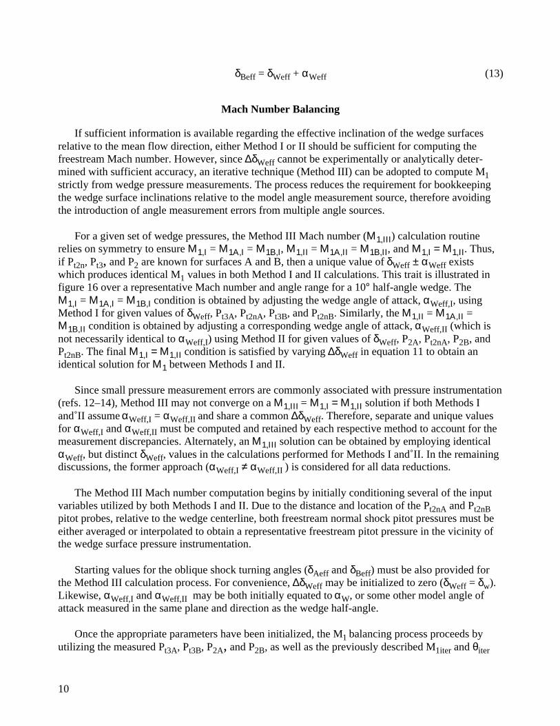
δBeff = δWeff + αWeff (13)

Mach Number Balancing

If sufficient information is available regarding the effective inclination of the wedge surfacesrelative to the mean flow direction, either Method I or II should be sufficient for computing thefreestream Mach number. However, since ∆δWeff cannot be experimentally or analytically deter-mined with sufficient accuracy, an iterative technique (Method III) can be adopted to compute M1strictly from wedge pressure measurements. The process reduces the requirement for bookkeepingthe wedge surface inclinations relative to the model angle measurement source, therefore avoidingthe introduction of angle measurement errors from multiple angle sources.

For a given set of wedge pressures, the Method III Mach number (Μ1,ΙΙΙ) calculation routinerelies on symmetry to ensure Μ1,Ι = Μ1Α,Ι = Μ1Β,Ι, Μ1,ΙΙ = Μ1Α,ΙΙ = Μ1Β,ΙΙ, and Μ1,Ι = Μ1,ΙΙ. Thus,if Pt2n, Pt3, and P2 are known for surfaces A and B, then a unique value of δWeff ± αWeff existswhich produces identical M1 values in both Method I and II calculations. This trait is illustrated infigure 16 over a representative Mach number and angle range for a 10° half-angle wedge. TheΜ1,Ι = Μ1Α,Ι = Μ1Β,Ι condition is obtained by adjusting the wedge angle of attack, αWeff,I, usingMethod I for given values of δWeff, Pt3A, Pt2nA, Pt3B, and Pt2nB. Similarly, the Μ1,ΙΙ = Μ1Α,ΙΙ =Μ1Β,ΙΙ condition is obtained by adjusting a corresponding wedge angle of attack, αWeff,II (which isnot necessarily identical to αWeff,I) using Method II for given values of δWeff, P2A, Pt2nA, P2B, andPt2nB. The final Μ1,Ι = Μ1,ΙΙ condition is satisfied by varying ∆δWeff in equation 11 to obtain anidentical solution for Μ1 between Methods I and II.

Since small pressure measurement errors are commonly associated with pressure instrumentation(refs. 12–14), Method III may not converge on a Μ1,ΙΙΙ = Μ1,Ι = Μ1,ΙΙ solution if both Methods Iand II assume αWeff,I = αWeff,II and share a common ∆δWeff. Therefore, separate and unique valuesfor αWeff,I and αWeff,II must be computed and retained by each respective method to account for themeasurement discrepancies. Alternately, an Μ1,ΙΙΙ solution can be obtained by employing identicalαWeff, but distinct δWeff, values in the calculations performed for Methods I and II. In the remainingdiscussions, the former approach (αWeff,I ≠ αWeff,II ) is considered for all data reductions.

The Method III Mach number computation begins by initially conditioning several of the inputvariables utilized by both Methods I and II. Due to the distance and location of the Pt2nA and Pt2nBpitot probes, relative to the wedge centerline, both freestream normal shock pitot pressures must beeither averaged or interpolated to obtain a representative freestream pitot pressure in the vicinity ofthe wedge surface pressure instrumentation.

Starting values for the oblique shock turning angles (δAeff and δBeff) must be also provided forthe Method III calculation process. For convenience, ∆δWeff may be initialized to zero (δWeff = δw).Likewise, αWeff,I and αWeff,II may be both initially equated to αW, or some other model angle ofattack measured in the same plane and direction as the wedge half-angle.

Once the appropriate parameters have been initialized, the M1 balancing process proceeds byutilizing the measured Pt3A, Pt3B, P2A, and P2B, as well as the previously described M1iter and θiter

11

start-up values, to compute the terms in the Method I and II M1 calculation routines. Residuals fromthe first computation cycle are used to update the iteration variables on the subsequent computa-tional cycle. This process is performed repeatedly until the Μ1,ΙΙΙ ≈ Μ1,Ι ≈ Μ1,ΙΙ has been obtained.The general calculation process for Method III is described in Appendix C, with sample numericalcalculations given in Appendix D.

POST-TEST DATA PROCESSING AND ANALYSIS

Post-test data processing and analysis were performed on an Apple Macintosh PowerPC G3computer. The computational algorithms for evaluating the wedge and cone-probe data weredeveloped using National Instruments LabVIEW software, which featured a high-level, graphicaluser interface (GUI) language with built-in analytical functions. Additional data processing wasaccomplished using Microsoft Excel’s spreadsheet and plotting functions.

TEST SECTION SURVEY RESULTS

Normal Shock Pitot Pressure Distribution

Figure 17 shows the settling chamber referenced normal shock pitot recovery distributions at thetest section vertical centerline (y = 24 in.) and constant horizontal stations (z = 16.24, 19.73 in.) forthe three Mach number settings. The pressures were mapped from separate Pt2nA and Pt2nB measure-ments obtained from the multiple wedge orientations depicted in figure 7. Variations in the localpitot pressure along the z-direction were greater than the estimated measurement uncertaintyassociated with the wedge pitot and settling chamber pressures. The distributions are indicative ofthe flow nonuniformity within the surveyed region of each respective test section.

Flow Angularity

The approach for determining the tunnel upflow, µ, and crossflow, ξ, relied on deriving thesensitivity of the wedge surface A to B static pressure ratio, P2A/P2B, to a corrected wedge angle ofattack, αWcorr. Since there was greater confidence in the pitch angle (ε) measurement accuracy,αWcorr was obtained from wedge pitch data runs only (φM = 0°, 180°, ψ = 0°). From this set of data,the corrected angle of attack was obtained by relating P2A/P2B to the wedge angle of attack, αW,defined by:

αW = εcos(φM)

As shown in figure 18, αWcorr represented the midpoint between upright and invertedαW – P2A/P2B polars at z = 16.24 in. and z = 19.73 in. for constant P2A/P2B. An analytical expres-sion describing αWcorr(P2A/P2B) for both wedge locations above the test section floor was obtainedat each Mach number through regression analysis. µ and ξ were determined by respectively relatingε and ψ to αWcorr(P2A/P2B) for each tunnel Mach number, as depicted in figure 19. The test section

12

flow angle was presumed to coincide with αWcorr(P2A/P2B) = 0° for wedge articulation in the pitchand yaw directions.

Figures 20 and 21, respectively, show the assumed linear upflow, µ(z), and crossflow, ξ(z),distributions extracted from wedge measurements at z = 16.24 in. and z = 19.73 in. at each tunnelMach number setting. UPWT TS 1 exhibited the largest upflow angle of nearly 1.5°. Crossflowvaried between ±0.2° in both test sections. The magnitudes and trends were in general agreementwith the nominal tunnel flow angles described in reference 6.

Mach Number and Pressure Recovery

In order to compute the freestream Mach number from the wedge pressures, a fourth-orderpolynomial regression was first applied to the normal shock pitot pressure distribution along thetest section centerline (y = 24 in.), shown in figure 17. This analytical representation describingPt2n(z)/Pt0 was used to interpolate Pt2n from wedge position information and tunnel settling chamberpressure, Pt0. Values for z were referenced to the wedge leading edge height above the test sectionfloor, and determined from zref(ε) in figure 10, together with wedge and sting adapter dimensions.

Establishing Pt2n from the spatial distribution was preferred over the numerical averaging ofPt2nA and Pt2nB due to the pressure measurement uncertainty associated with the lateral separationdistance between the outboard pitot probes and wedge surface instrumentation. As shown infigure 22, the analytical Pt2n(z)/Pt0 distribution gave a better approximation of the normal shockpressure within close proximity of the wedge surface static and pitot instrumentation.

Figure 23 compares the Method I, II, and III Mach numbers with the ideal Mach numbercomputed from Pt2n(z)/Pt0 using equation 5 (assuming perfect recovery, Pt1 = Pt0). To precludethe introduction of errors associated with flow angularity, the assumed linear distributions wereconstructed from measurements made within ±0.25° of the computed upflow and crossflow angles ateach wedge position above the test section floor. The Mach gradient for all methods was steepest forTS 2 at Mset = 2.29, with the Mach number being higher at the survey location closest to the tunnelfloor.

Ideally, the test section Mach number should have been identical for all calculation methods atall flow conditions. At a tunnel Mach setting of 2.15 in TS 1, the Mach numbers for Methods I, II,and III were reasonably close to each other, with the exception of the ideal Mach, which was higherthan the others, as would be expected. However, the Method I, II, and III–computed Mach numbersfor TS 2 diverged with increasing Mach. At Mset = 2.40, the Method I Mach number exceeded theideal Mach value. Excluding the ideal Mach number, the Method III approach was an overallcompromise between Method I and II results.

The freestream total pressure recovery, Pt1/Pt0, computed from the corresponding Mach numbermethods and Pt2n(z)/Pt0 using equation 5 is shown in figure 24. Similar to the Mach number, linearpressure recovery distributions in the z-direction were defined by data within ±0.25° of the com-puted tunnel flow angles. The recovery trends reflected the variations in Mach number obtained

13

from Methods I, II, and III. At Mset = 2.40, the total pressure recovery computed from the Method IMach number was greater than unity, yielding overshoots on the order of 1 to 1.5%.

Wedge Measurement Discrepancies

Figure 25 shows the viscous flow deflection increment, ∆δWeff, resulting from the Method IIIcalculation process for the various wedge roll orientations as a function of wedge tip position abovethe test section floor. The largest increment is on the order of +0.3° at Mset = 2.40. However, atMach number settings of 2.15 and 2.29, the increment is less than zero. A positive wedge half-angleincrement could be explained as the effective boundary layer displacement on the wedge surfacesensed by the pressure instrumentation. For negative half-angle increments at the mid and lowerMach number settings, other contributing factors must be taken into account.

One plausible explanation for the observed anomaly considers the Mach number sensitivity towedge surface inclination and pressure measurement errors. The Mach number sensitivity topressure variations is compared between Methods I and II in figure 26. Referring to figure 13, thecurves are representative of the experimental flow conditions and wedge surface inclinations. Thesensitivities were obtained by evaluating the governing equations for the Method I and II Machnumber using central-differencing approximations.

The Method I Mach number sensitivity to the surface pitot pressure error, (∆M1/M1)/(∆Pt3/Pt3),decreases with increasing wedge deflection angle, and is relatively invariant with Mach number at agiven wedge angle. In contrast, the Method II Mach number sensitivity to the surface static pressureerror, (∆M1/M1)/(∆P2/P2), becomes increasingly negative with increasing wedge deflection angleand Mach number. The increasing magnitude of the Method II Mach number sensitivity with Machnumber could explain the method-dependent variations observed in figure 23.

In general, pitot pressures are less susceptible than surface static pressures to measurement errorsfrom instrumentation misalignment or geometry (ref. 12). Static pressures are strongly influenced byorifice size, rounding or chamfering, flushness, and hole alignment (ref. 14). Depending on thewedge surface inclination and Mach number, such static pressure measurement errors could haveadversely affected the computed Mach number, possibly accounting for total pressure recoveriesgreater than unity and the negative values of ∆δWeff, described above.

The Method III Mach number calculation technique assumes equal weighting of pressuremeasurement error between the wedge surface static and pitot instrumentation. Determining themagnitude of these errors and the proper weighting in the Method III calculations would haverequired additional experimental testing, which was beyond the scope of the test section flow surveyobjectives.

CONE-PROBE PERFORMANCE COMPARISONS

Figure 27 shows the static to pitot pressure ratio pitch polars (for taps A and C) for the initial16-probe cone-probe rake assembly tested at Mset = 2.40 and ψ = 0°. Theoretically, the polar shapefor each static pressure tap should have been continuous over the entire ±12° pitch range. Successful

14

correlation of the cone-probe angle of attack to the measured pressures was critically dependent onthis trait. However, it is evident from the figure that probes located near the center of the 4-by-4array (probes 2, 3, 6, 7, and 10) had polars which departed from the desired trends, exhibiting erraticchanges in magnitude between consecutive data points. Similar pressure polar behavior was alsoobserved at Mach numbers of 2.15 and 2.29 and in the transverse probe taps, B and D, as well.Figure 28 illustrates the relationship between the location of the affected probes and the downstreamblockage area in the 16-probe rake body.

Figures 29 and 30 show the static tap pressure polars for the respective 8- and 6-probe rakes atMset = 2.40 and ψ = 0°. Unlike the 16-probe rake, the pressure polar discontinuities were absentfrom the modified rakes at all flow conditions. The shadowgraphs in figure 31 illustrate thequalitative differences in the flow structure between the 16-probe rake and the modified rakes atvarious tunnel Mach settings. Although the incident shocks shed by the probe tips in the 16-proberake did not appear to impinge on the pressure-instrumented conical surface between adjacentprobes, the flow between the probes appeared chaotic and populated by multiple shock reflectionsand waves. Similar qualities were also observed in the 4-by-4 probe array at other Mach numbersand rake orientations. In contrast, the incident and reflected shocks from the probe tips on rakes 1and 2 were coherent and well-defined. Disturbances which plagued the static pressure taps on the16-probe rake were apparently attenuated by the reduced probe density, increased probe length, andaddition of rake body slots.

CONE-PROBE CALIBRATION

Reference Flow Conditions

The cone-probes were calibrated against the local test section flow distribution derived from thewedge measurements in the z-direction. From cone-probe rake dimensions and the relationshipshown in figure 10, z represented the distance from the test section floor to each probe tip, and wasdetermined from zref(ε), together with rake, probe, and sting adapter dimensions. Using this relation-ship, the cone-probe measurements could be referenced to the local test section flow angles, µ(z) andξ(z), Mach number, M1(z), and total pressure recovery, Pt1(z)/Pt0, based on the respective lineardistributions shown in figures 20, 21, 23, and 24. M1(z) and Pt1(z)/Pt0 were established from theMethod III calculation results. The coefficients representing the linear test section flow distributionfor µ(z), ξ(z), M1(z), and Pt1(z)/Pt0 are tabulated in table 1.

The effective cone-probe angles of attack, αC, and sideslip, βC, were calculated from the cosinetransformation of Euler angles expressed in terms of the known angles µ(z), ξ(z), ε, ψ, and φM,following the angle convention illustrated in figure 32:

15

tantan cos

cossin tan

tantan sin

coscos tan

αε ε φ

ψ ξφ ψ ξ

βε ε φ

ψ ξφ ψ ξ

CF M

M

CF M

M

zz

zz

=+( )

− ( )[ ] + − ( )[ ]

=+( )

− ( )[ ] − − ( )[ ](14)

where

tan tan cosε µ ξF z z= ( ) ( )

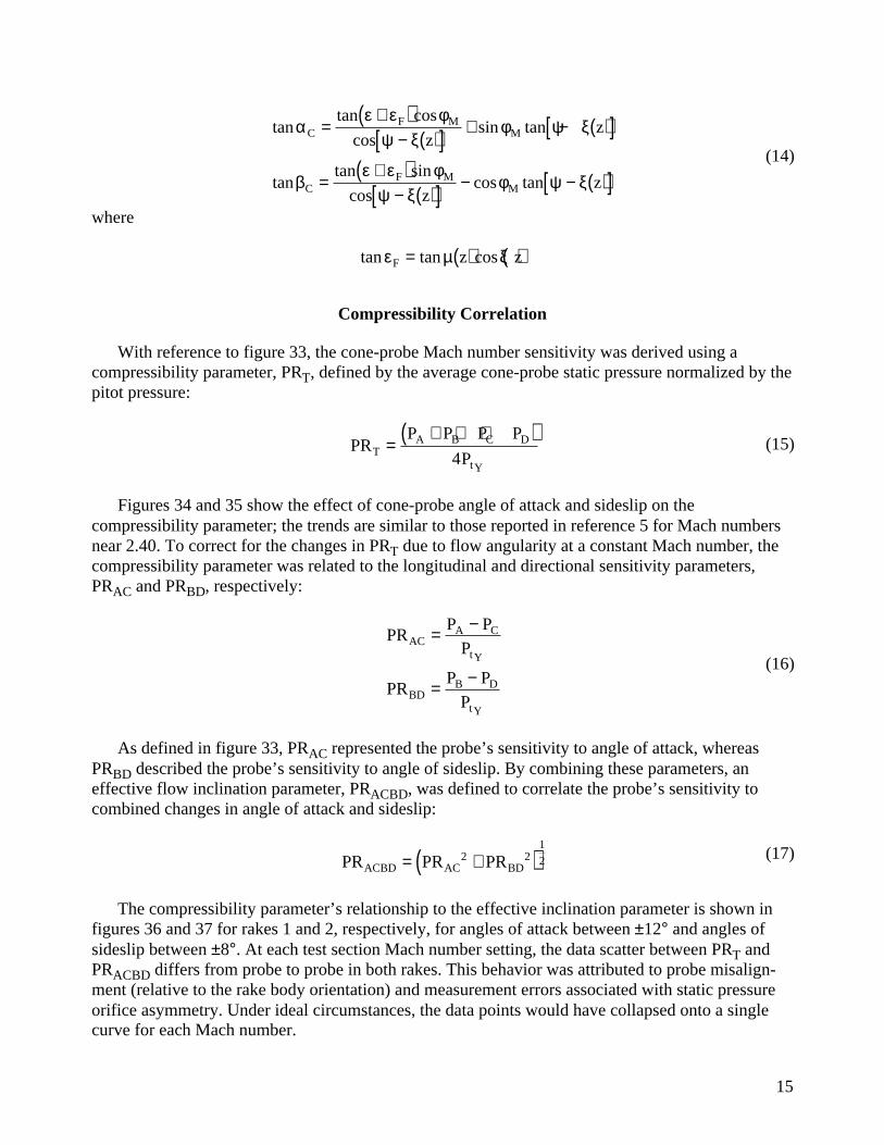
Compressibility Correlation

With reference to figure 33, the cone-probe Mach number sensitivity was derived using acompressibility parameter, PRT, defined by the average cone-probe static pressure normalized by thepitot pressure:

PRP P P P

PTA B C D

tY

=+ + +( )

4(15)

Figures 34 and 35 show the effect of cone-probe angle of attack and sideslip on thecompressibility parameter; the trends are similar to those reported in reference 5 for Mach numbersnear 2.40. To correct for the changes in PRT due to flow angularity at a constant Mach number, thecompressibility parameter was related to the longitudinal and directional sensitivity parameters,PRAC and PRBD, respectively:

PRP P

P

PRP P

P

ACA C

tY

BDB D

tY

= −

= −(16)

As defined in figure 33, PRAC represented the probe’s sensitivity to angle of attack, whereasPRBD described the probe’s sensitivity to angle of sideslip. By combining these parameters, aneffective flow inclination parameter, PRACBD, was defined to correlate the probe’s sensitivity tocombined changes in angle of attack and sideslip:

PR PR PRACBD AC BD= +( )2 21

2 (17)

The compressibility parameter’s relationship to the effective inclination parameter is shown infigures 36 and 37 for rakes 1 and 2, respectively, for angles of attack between ±12° and angles ofsideslip between ±8°. At each test section Mach number setting, the data scatter between PRT andPRACBD differs from probe to probe in both rakes. This behavior was attributed to probe misalign-ment (relative to the rake body orientation) and measurement errors associated with static pressureorifice asymmetry. Under ideal circumstances, the data points would have collapsed onto a singlecurve for each Mach number.

16

To improve the correlation between the compressibility and inclination parameters described byequation 17, the effective inclination parameter was redefined to account for probe misalignmenteffects and pressure tap errors by introducing a corrected inclination parameter, PRACBDcorrT:

PR PR PR PR PRACBDcorrT AC ACbiasT BD BDbiasT= +( ) + +( )

2 21

2 (18)

PRACbiasT and PRBDbiasT were bias components in the respective cone-probe longitudinal anddirectional sensitivity parameters, and were assumed to be unique for each probe and invariant withflow angle at a constant Mach number. For data obtained at a constant Mset, these bias terms weredetermined by parametrically adjusting PRACbiasT and PRBDbiasT in equation 18 until the standarddeviation for a cubic regression relating PRT to PRACBDcorrT converged to acceptable levels. Theanalytical expression which was found to yield the least PRT data scatter for all probes took thefollowing implicit form:

PRT = lT0 + lT1xT + lT2xT2 + lT3xT

3, where xT = PRACBDcorrT PRT7 (19)

Since data irregularities were present at extreme angles of attack and compromised the overallquality of the regression, the numerical analysis was limited to cone-probe angles of attack andsideslip within ±8°. Curves of PRT(PRACBDcorrT) obtained from the PRACbiasT and PRBDbiasTiteration using equation 19 are shown in figures 38 and 39 for rakes 1 and 2, respectively.

Once the compressibility parameter had been correlated to the corrected inclination parameter,the effects of flow angularity was established. Referring to figure 40, the offset coefficient, lT0, inequation 19 defined the fundamental compressibility parameter, PRT0, which was assumed to beinvariant with flow angularity and dependent only on Mach number. The remaining higher orderterms represented the flow angularity increment, ∆PRT, to the fundamental compressibilityparameter. After rearranging and substituting terms in equation 19, the fundamental compressibilityparameter was expressed as:

PRT0 = PRT - ∆PRT = PRT – (lT1xT + lT2xT2 + lT3xT

3) (20)

Since the cone-probes had been calibrated at three separate tunnel Mach number settings (2.15,2.29, and 2.40), three corresponding values of PRT0 were obtained for each cone-probe to expressPRACbiasT, PRBDbiasT, lT1, lT2, and lT3 as quadratic functions of PRT0:

PRACbiasT = jT0 + jT1 PRT0 + jT2 PRT02

PRBDbiasT = kT0 + kT1 PRT0 + kT2 PRT02

lT1 = mT0 + mT1 PRT0 + mT2 PRT02

lT2 = nT0 + nT1 PRT0 + nT2 PRT02

lT3 = qT0 + qT1 PRT0 + qT2 PRT02

17

The second-order coefficients for PRACbiasT, PRBDbiasT, lT1, lT2, and lT3 are listed in tables 2and 3 for rakes 1 and 2, respectively.

By assuming that PRACbiasT, PRBDbiasT, lT1, lT2, and lT3 were solely dependent on PRT0 for eachprobe, PRT0 was determined by numerically solving the resulting implicit relation in equation 20:

PRT – (lT1xT + lT2xT2 + lT3xT

3) – PRT0 = 0 (21)

A sample calculation for PRT0 is included in Appendix E.

Mach Number Correlation

The Mach number was correlated to the cone-probe pressures following the general methodemployed in reference 5, which expressed the Mach number as an empirical function of thecompressibility parameter at zero flow incidence. Consequently, M1(z) was explicitly derived as afunction of the fundamental compressibility parameter to eliminate the effects of flow angularity.Since the calibration data was obtained at Mach numbers of 2.15, 2.29, and 2.40, the correlationaccuracy was dependent on the analytical relationship between M1(z) and PRT0. From conical shockrelations provided reference 11, values for the freestream Mach number were computed for a 40°cone as a function of the theoretical PRT0 to extrapolate for conditions beyond the experimentalMach number range. A polynomial regression of the collective data set containing both experimentaland supplemental data expressed the calibrated cone-probe Mach number, M1Ccal, as a fourth-orderpolynomial function of the fundamental compressibility parameter:

M1Ccal = CM0 + CM1 PRT0 + CM2 PRT02+ CM3 PRT0

3+ CM4 PRT04 (22)

The coefficients derived for M1Ccal are listed in table 4 for both cone-probe rakes.

Figures 41 and 42 illustrate the analytical Mach number dependency on the fundamentalcompressibility parameter for rakes 1 and 2, respectively. The two-standard deviation, 2σ(M1Ccal),calculated from the residuals between M1Ccal and M1(z) is shown in figures 43 and 44 for rakes 1and 2, respectively. This statistic was a general measure of the cone-probe Mach number resolution,rather than an indicator of the absolute Mach number calibration accuracy. The calibrated Machnumber residuals were within a 2σ(M1Ccal) of ±0.01 for Mach numbers above 2.29. Probes 5 and 6on rake 1 and probe 3 on rake 2 exhibited higher M1Ccal deviations at Mset = 2.15 over the ±8° angleof attack and sideslip range.

Total Pressure Correlation

Figures 45 and 46 show the effect of cone-probe angle of attack and sideslip on thecompressibility parameter; the trends are similar to those reported in ref. 5 for Mach numbers near2.40. Similar to the compressibility parameter, the cone-probe pitot pressure, PtY, was correlated toPRACBD to represent the variation with flow angularity. Figures 47 and 48 show the pitot pressurevariation with the effective inclination parameter for rakes 1 and 2, respectively, at constant tunnelMach numbers. The data scatter was considered an artifact of both probe misalignment and

18

measurement error due to probe inclination to the mean flow direction. This behavior has beenobserved for sharp-edged pitot probes with conical tips (ref. 13).

To improve the correlation between the pitot pressure and inclination parameter, an effectiveinclination parameter, PRACBDcorrY, was introduced to correct for probe misalignment effects andflow angularity at a constant Mach number:

PR PR PR PR PRACBDcorrY AC ACbiasY BD BDbiasY= +( ) + +( )

2 2(23)

The relationship between PtY and PRACBDcorrY was based on the model presented in figure 49.The pitot pressure variation was expressed in terms of ∆PtY/PtY, which analytically described thedeviation from the maximum pitot pressure due to flow inclination at constant Mach number. As inthe compressibility parameter correlation, PRACbiasY and PRBDbiasY were the bias offsetscomplementing the respective cone-probe longitudinal and directional sensitivity parameters, andaccounted for the PtY data scatter with flow inclination at a constant Mach number. For dataobtained at a constant Mset, these bias terms were determined for each cone-probe by parametricallyadjusting PRACbiasY and PRBDbiasY in equation 23 until the standard deviation for a cubic regressionrelating ∆PtY/PtY to PRACBDcorrY converged to within acceptable levels. The cubic relationship tookthe following form:

∆PtY/PtY = lY0 + lY1xY + lY2xY2 + lY3xY

3, where xY = PRACBDcorrY (24)

For each iteration cycle, ∆PtY/PtY was determined from a separate cubic regression ofPtY(PRACBDcorrY):

PtY = lYabs0 + lYabs1xY + lYabs2xY2 + lYabs3xY

3 (25)

From this expression, PtYmax, the maximum value of PtY(PRACBDcorrY) for xY ≥ 0, wasdetermined; for positive, real values of xY, PtYmax was derived by solving equation 25 for xYmaxwhich yielded the maximum PtY(PRACBDcorrY):

xl l l l

lYYabs Yabs Yabs Yabs

Yabsmax

=− + −

2 22

1 3

3

3

3(26)

Then

PtYmax = lYabs0 + lYabs1xYmax + lYabs2xYmax2 + lYabs3xYmax

3

Otherwise, PtYmax = lYabs0 for non-real or negative values of xY. Once PtYmax was computed,∆PtY/PtY could be calculated to evaluate equation 24:

∆PtY/PtY = PtYmax/PtY – 1 (27)

19

Similar to the PRT analysis, the analysis of ∆PtY/PtY(PRACBDcorrY) and PtYmax was limited tonominal cone-probe angles of attack and sideslip within ±8°. Curves of PtY/Pt0(PRACBDcorrY)resulting from the converged solution of equation 24 are shown in figures 50 and 51 for rakes 1and 2, respectively.

To account for compressibility effects, PRACbiasY, PRBDbiasY, lY0, lY1, lY2, and lY3 wereexpressed as analytical functions of PRT0 for each probe. Since the cone-probes were calibrated atthree separate tunnel Mach numbers (2.15, 2.29, and 2.40), PRACbiasY, PRBDbiasY, lY0, lY1, lY2, andlY3 were related to the three corresponding values of PRT0 using a second-order polynomial functionobtained through regression analysis:

PRACbiasY = jY0 + jY1 PRT0 + jY2 PRT02

PRBDbiasY = kY0 + kY1 PRT0 + kY2 PRT02

lY0 = mY0 + mY1 PRT0 + mY2 PRT02

lY1 = nY0 + nY1 PRT0 + nY2 PRT02

lY2 = qY0 + qY1 PRT0 + qY2 PRT02

lY3 = rY0 + rY1 PRT0 + rY2 PRT02

The second-order coefficients for PRACbiasY, PRBDbiasY, lY0, lY1, lY2, and lY3 resulting from theminimization of ∆PtY/PtY (PRACBDcorrY) at each Mach number are listed in tables 5 and 6 forrakes 1 and 2, respectively.

Once the flow inclination correction had been obtained, the corrected pitot pressure, PtYcorr, wasequated to PtYmax and solved by combining equations 24 and 27:

PtYcorr = (1 + lY0 + lY1xY + lY2xY2 + lY3xY

3)Pt Y (28)

From PtYcorr and the explicit relation for M1Ccal given in equation 22, the calibrated cone-probefreestream total pressure, Pt1Ccal, was calculated from the one-dimensional normal shock equation:

P PM

M

Mt Ccal tYcorr

Ccal

Ccal

Ccal1

12

12

7

21

25

25

6

7 1

6=

+

−

(29)

The two-standard deviation, 2σ(Pt1Ccal/Pt0), of the residuals between the calibrated cone-probetotal pressure recovery, Pt1Ccal/Pt0, and the reference test section total pressure recovery distribution,Pt1(z)/Pt0, is depicted in figures 52 and 53 for rakes 1 and 2, respectively. This statistic was a generalmeasure of the correlation’s ability to resolve the freestream total pressure, rather than an indicatorof the absolute total pressure calibration accuracy. The calibrated total pressure recovery residualswere typically within a 2σ(Pt1Ccal/Pt0) of ±0.01 (±1% of the settling chamber pressure) for Mach

20

numbers above 2.29. On most probes, the deviation between the cone-probe and wedge-surveyedfreestream pressure recovery remained relatively invariant with probe angle of attack and sideslip.Probes 5 and 6 on rake 1 and probes 1 and 3 on rake 2 exhibited higher Pt1Ccal/Pt0 deviations atMset = 2.15 over the ±8° angle of attack and sideslip range.

Angle of Attack Correlation

Due to the size and arrangement of the probes in the rake assembly, the actual angle of attack foreach cone-probe could not be directly measured with sufficient accuracy. For simplicity, the angle ofattack for each probe was referenced to its effective angle of attack, αC. Since any probe misalign-ment relative to the αC reference datum was most likely to be small, any probe offset angle in thepitch direction would presumably appear as a bias error in the cone-probe pressures. Referring tofigure 32, αC was approximately proportional to the longitudinal sensitivity parameter, PRAC. Thisobservation is illustrated in figures 54 and 55 for rakes 1 and 2, respectively, at a nominal angle ofsideslip of 0° and tunnel Mach number of 2.40. Similar trends were exhibited at other Machnumbers as well.

To avoid increased fit errors from data irregularities at higher angles, the cone-probe angle ofattack analysis was limited to data within a model pitch range of ±8°. From this reduced data set, thecalibrated cone-probe angle of attack, αCcal, was analytically correlated to the measured cone-probepressures in the following manner:

αCcal = α0 – ∆αB – ∆αcorr (30)

The first term on the right side of equation 30 represented the linear variation of the effectivecone-probe angle of attack with the longitudinal sensitivity parameter. α0 was derived from theregression of αC with PRAC at a nominal βC of zero for each tunnel Mach number setting:

α0 = a0 + a1PRAC (31)

The second term in equation 30 corrected for probe angle of attack variations due to crossflow.For each data run at a nominally constant ψ, ∆αB was determined from a fourth-order polynomialregression relating (αC – α0) to PRAC at a constant Mset:

∆αB = αC – α0 = b0+ b1 PRAC + b2P PRAC2+ b3 PRAC

3+ b4 PRAC4 (32)

Since PRBD was assumed to be nearly invariant with angle of attack, each coefficient inequation 32 was correlated to the average directional sensitivity parameter, PRBDavg, using a sixth-order regression of the form:

bi = c0i + c1i PRBDavg + c2i PRBDavg2 + c3i PRBDavg

3 + c4i PRBDavg4 + c5i PRBDavg

5

+ c6i PRBDavg6 (33)

where i = 0 to 4

21

For each cone-probe, PRBDavg was computed at a nominally constant ψ for each tunnel Machnumber condition.

The last term in equation 30 corrects for any residuals resulting from the αC, α0, and ∆αBrelationship with PRAC at a constant Mset:

∆αcorr = α0 – αC – ∆αB = d0+ d1PRAC+ d2PRAC2+ d3PRAC

3+ d4PRAC4 (34)

To capture the αC sensitivity to Mach number, the a, c, and d coefficients obtained at each of thethree tunnel Mach numbers (2.15, 2.29, and 2.40) were analytically related to the correspondingvalues of PRT0 using a quadratic function obtained from regression analysis:

a0 = C0,a0 + C1,a0 PRT0 + C2,a0 PRT02

a1 = C0,a1 + C1,a1 PRT0 + C2,a1 PRT02

c0i = C0,c0 + C1,c0 PRT0 + C2,c0 PRT02

c1i = C0,c1 + C1,c1 PRT0 + C2,c1 PRT02

c2i = C0,c2 + C1,c2 PRT0 + C2,c2 PRT02

c3i = C0,c3 + C1,c3 PRT0 + C2,c3 PRT02

c4i = C0,c4 + C1,c4 PRT0 + C2,c4 PRT02

c5i = C0,c5 + C1,c5 PRT0 + C2,c5 PRT02

c6i = C0,c6 + C1,c6 PRT0 + C2,c6 PRT02

d0 = C0,d0 + C1,d0 PRT0 + C2,d0 PRT02

d1 = C0,d1 + C1,d1 PRT0 + C2,d1 PRT02

d2 = C0,d2 + C1,d2 PRT0 + C2,d2 PRT02

d3 = C0,d3 + C1,d3 PRT0 + C2,d3 PRT02

d4 = C0,d4 + C1,d4 PRT0 + C2,d4 PRT02

The second-order coefficients for a, c, and d are listed in tables 7 and 8 for rakes 1 and 2,respectively.

The two-standard deviation, 2σ(αCcal), calculated from the residual between αCcal and αC isshown in figures 56 and 57 for rakes 1 and 2, respectively. Similar to the Mach number and totalpressure results, this statistic was a general measure of the correlation method’s ability to resolve the

22

cone-probe angle of attack, rather than being an indicator of the absolute angle of attack calibrationaccuracy. Over the ±8° angle of attack and sideslip range, the effective cone-probe angle of attackresiduals were within a 2σ(αCcal) of ±0.1°. For most probes, the deviation between the calibratedcone-probe angle of attack and αC remained relatively invariant with probe angle of attack andsideslip. Most excursions from this trend occurred at the extreme probe attitude angles and at thetunnel Mach number setting of 2.15.

Angle of Sideslip Correlation

Similar to the angle of attack correlation, the angle of sideslip for each cone-probe wasreferenced to the effective angle of sideslip, βC. As a consequence, any probe misalignment in theyaw direction would appear as a bias error in the local cone-probe pressures. Referring to figure 32,βC was nominally proportional to the directional sensitivity parameter, PRBD. This observation isillustrated in figures 58 and 59, which are the respective cross-plots of figures 54 and 55 for rakes 1and 2 at a nominal angle of attack of 0° and tunnel Mach number of 2.40. Similar trends were alsoobtained at other Mach numbers.

To avoid increased fit errors from data irregularities at higher angles, the cone-probe angle ofsideslip analysis was limited to data within a model pitch range of ±8°. From this reduced data set,the calibrated cone-probe angle of sideslip, βCcal, was analytically correlated to the measured cone-probe pressures in the following manner:

βCcal = β0 – ∆βA – ∆βcorr (35)

The first term on the right side of equation 35 described the linear variation of βC with PRBD.β0 was derived from the regression of βC with PRBD at a nominal angle of attack of zero for eachtunnel Mach number condition:

β0 = e0 + e1PRBD (36)

The second term in equation 35 corrected for probe angle of sideslip variations due to angle ofattack. ∆βA was determined from a fourth-order polynomial regression relating (βC – β0) to PRBD ata constant Mset and angle of attack:

∆βA = βC – β0 = f0+ f1PRBD+ f2PRBD2+ f3PRBD

3+ f4PRBD4 (37)

Since PRAC was assumed to be nearly invariant with angle of sideslip, each coefficient inequation 37 was correlated to an average longitudinal sensitivity parameter, PRACavg, using a sixth-order regression of the form:

fi = g0i + g1i PRACavg + g2i PRACavg2 + g3i PRACavg

3 + g4i PRACavg4 + g5i PRACavg

5

+ g6i PRACavg6 (38)

where i = 0 to 4

23

For each cone-probe, PRACavg was computed at a nominally constant ε for each tunnel Machnumber condition.

The last term in equation 35 corrected for any residuals, which resulted from relating βC, β0,and ∆βA to PRBD at a constant tunnel Mach number:

∆βcorr = β0 – βC – ∆βA = h0+ h1PRBD+ h2PRBD2+ h3PRBD

3+ h4PRBD4 (39)

To capture the βC sensitivity to Mach number, the e, g, and h coefficients obtained at each of thethree tunnel Mach numbers (2.15, 2.29, and 2.40) were analytically related to the correspondingvalues of PRT0 using a quadratic function obtained from regression analysis:

e0 = C0,e0 + C1,e0 PRT0 + C2,e0 PRT02

e1 = C0,e1 + C1,e1 PRT0 + C2,e1 PRT02

g0i = C0,g0 + C1,g0 PRT0 + C2,g0 PRT02

g1i = C0,g1 + C1,g1 PRT0 + C2,g1 PRT02

g2i = C0,g2 + C1,g2 PRT0 + C2,g2 PRT02

g3i = C0,g3 + C1,g3 PRT0 + C2,g3 PRT02

g4i = C0,g4 + C1,g4 PRT0 + C2,g4 PRT02

g5i = C0,g5 + C1,g5 PRT0 + C2,g5 PRT02

g6i = C0,g6 + C1,g6 PRT0 + C2,g6 PRT02

h0 = C0,h0 + C1,h0 PRT0 + C2,h0 PRT02

h1 = C0,h1 + C1,h1 PRT0 + C2,h1 PRT02

h2 = C0,h2 + C1,h2 PRT0 + C2,h2 PRT02

h3 = C0,h3 + C1,h3 PRT0 + C2,h3 PRT02

h4 = C0,h4 + C1,h4 PRT0 + C2,h4 PRT02

The second-order coefficients for e, g, and h are listed in tables 9 and 10 for rakes 1 and 2,respectively.

The two-standard deviation, 2σ(βCcal), calculated from the residuals between βCcal and βC isshown in figures 60 and 61 for rakes 1 and 2, respectively. As with the other cone-probe parameters,this statistic quantified the angle of sideslip resolution for the correlation method, rather than serving

24

as a measure of the absolute angle of sideslip calibration accuracy. Over the ±8° angle of attack andsideslip range, the effective cone-probe angle of sideslip residuals were within a 2σ(βCcal) of ±0.1°.The deviation between the calibrated cone-probe angle of sideslip and βC remained relativelyinvariant with probe angle of attack and sideslip on both rakes. Most excursions from thisobservation occurred at the extreme probe attitude angles.

UNCERTAINTY ANALYSIS

General Measurement Accuracy

Performing a comprehensive, end-to-end uncertainty analysis for each instrument and dataacquisition process was essentially impractical. Instead, reasonable engineering judgments weremade as to which measurement variables were most likely have a significant impact on the testsection flow survey and cone-probe calibration quality. In many circumstances, various quality andcontrol procedures were instituted prior to and during wind tunnel testing to ensure experimentaldeviations were within acceptable limits. Calibration information and test data pertaining to thedominant error sources were evaluated for propagating the measurement uncertainties into thecomputed results. Instrument and calibration working standard accuracies were estimated fromUPWT installed calibration results and archived Langley metrology data. Comparisons with themanufacturer’s specifications were made to assess the short-term accuracy and long-term stability ofthe measurement device, relative to the duration of each particular wind tunnel test entry. In allcases, the most conservative (highest uncertainty) figures were assumed in the analyses.

Uncertainties were estimated at the 95% confidence level, following the methods established inrefs. 14–16. The total measurement uncertainty was expressed as the root-sum-square (RSS) of thebias and precision limits. Where applicable, correlated bias limits were included for measurementvariables and computed parameters sharing common data paths or reference sources. A coveragefactor of 2 was applied in estimating the precision limits for each independent measurementvariable. Partial derivatives involving complex, implicit equations or recursive algorithms wereevaluated using second-order accurate, central-difference approximations; the computationalstepsizes were evaluated and selected to avoid numerical round-off errors, while minimizing theapproximation error due to truncation (ref. 17).

Table 11 summarizes the estimated uncertainty for the measurement devices employed for bothwedge and cone-probe tests. The tabulated results are limited to the static (wind-off) performance ofthe data acquisition devices and equipment. The estimates exclude errors associated with dynamicphenomena typically experienced during actual wind-on testing, such as flow unsteadiness, heattransfer, and vibration. The effects of pressure tubing delay time on sampling duration, gravimetricpressure variations (due to transducer elevation above/below test article) and leakage during testsection depressurization were also neglected from these estimates.

25

Test Section Flow Angularity Uncertainties

The test section upflow uncertainty, Uµ, was estimated from a combination of the regressionresiduals produced by the ε−αWcorr relationships (shown in fig. 19) and the measurement uncertaintyof ε. Figure 62 shows the overall data scatter about the analytical expression for ε(αWcorr), with theerror bars representing the total uncertainty in ε based on the static performance of the Q-flexaccelerometer. Within ±0.5° of the presumed local upflow direction, Uµ was estimated to be ±0.05°in the surveyed region of each test section for all Mach number settings. Since the wedge wasrepeatedly tested at selected conditions, the random deviations represent the short- and mid-termdata repeatability. Compared to the size of the error bars, the relatively larger data scatter indicatesthe upflow uncertainty comprised mostly wind-on data precision error.

Similar to the upflow uncertainty, the test section crossflow uncertainty, Uξ, was estimated froma combination of the regression residuals resulting from the ψ−αWcorr correlation (shown in fig. 19)and the measurement uncertainty of ψ. Figure 63 shows the deviations about the analytical functionfor ψ(αWcorr), with the error bars representing the total uncertainty in ψ based on the static perfor-mance of the tunnel strut yaw mechanism. Within ±0.5° of the presumed local crossflow direction,Uξ was estimated to be ±0.12° in the surveyed region of both test sections for all Mach numbersettings. In contrast to the upflow error, the static measurement uncertainty for ψ dominated thewind-on measurement precision error, as characterized by the relative difference in magnitudesbetween the error bars and the data scatter.

Test Section Mach and Recovery Uncertainties

The test section Mach number uncertainty (UM1) and total pressure recovery uncertainty(UPt1/Pt0) were estimated from the residuals about their respective linear distributions, shown infigures 23 and 24. The propagation of the wind-off pressure measurement bias and precision limitsinto the Method III Mach number computation algorithm were included.

Figure 64 shows the Method III Mach number deviation about the presumed linear distribution,with error bars representing the computational variations resulting from the pressure measurementuncertainties. For data acquired at wedge orientations within ±0.25° of the presumed local upflowand crossflow directions, UM1 was estimated to be ±0.005 in the surveyed region of each test sectionfor all Mach number settings. The comparable size of the error bars and data scatter indicates theMach number uncertainty was equally composed of both wind-on measurement precision andcalculation errors.

Figure 65 shows the total pressure recovery scatter about the presumed linear distribution, witherror bars representing the computational variations resulting from the pressure measurementuncertainties. For data acquired at wedge orientations within ±0.25° of the presumed local upflowand crossflow directions, UPt1/Pt0 was estimated to be ±0.01 (±1% of Pt0) in the surveyed region ofeach test section for all Mach number settings. Unlike the Mach number uncertainty, the totalpressure recovery uncertainty was dominated by calculation errors arising from the propagatedpressure measurement uncertainties.

26

Although disparities existed between the Method I and II Mach number and total pressurerecovery results, these deviations were excluded from the uncertainty analysis, since they wereby-products of the interim solutions leading to the Method III results. Uncertainties from wedgepitot and static pressure measurement errors resulting from probe and orifice geometry were alsoneglected from the analyses, since these effects could not be quantified without additionalexperimental work.

Cone-Probe Mach Number and Pressure Recovery Uncertainties

The absolute uncertainty of the calibrated cone-probe Mach number (UM1c) was estimated fromthe M1Ccal correlation residuals, the uncertainty of the reference Mach number (UM1), and theuncertainty resulting from the propagation of the wind-off bias and precision limits into the M1Ccalcalculations. UM1c was estimated as the sum of 2σ(M1Ccal) and the RSS of UM1 and a statisticrepresenting the nominal M1Ccal calculation uncertainty. The latter term was expressed as the sum ofthe average and two-standard deviation of the calculation uncertainties computed from all datapoints contained within a prescribed cone-probe angle of attack and sideslip range.

The variation of UM1c over selected ranges of cone-probe angles of attack and sideslip ispresented in figures 68 and 69 for rakes 1 and 2, respectively. For many probes, the calculationuncertainty accounted for the majority of UM1c, and was primarily due to the sensitivity of PRT0 andM1Ccal to small cone-probe pressure changes. The absolute uncertainty in the calibrated cone-probeMach number generally increased with increasing Mach number, typically ranging from ±0.01 to±0.04 for both rakes.

Similar to the Mach number uncertainty, the absolute uncertainty of the calibrated cone-probetotal pressure recovery (UPt1c/Pt0) was estimated from correlation residuals for Pt1Ccal/Pt0, theuncertainty of the reference test section total pressure recovery (UPt1/Pt0), and the uncertaintyresulting from the propagation of the wind-off bias and precision limits through the Pt1Ccal/Pt0calculation process. UPt1c/Pt0 was estimated as the sum of 2σ(Pt1Ccal/Pt0) and the RSS of UPt1/Pt0 anda statistic representing the nominal Pt1Ccal/Pt0 calculation uncertainty. The last uncertainty compo-nent was the sum of the average and two-standard deviation of the calculation uncertainty computedfrom all data points contained within a prescribed cone-probe angle of attack and sideslip range.

The variation of UPt1c/Pt0 over selected ranges of cone-probe angles of attack and sideslip isshown in figures 68 and 69 for rakes 1 and 2, respectively. For all probes on both rakes, thecalculation uncertainty accounted for nearly all of UPt1c/Pt0, and was approximately an order ofmagnitude greater than the correlation resolution defined by 2σ(Pt1Ccal/Pt0). The relatively largePt1Ccal/Pt0 calculation uncertainty resulted from the accumulation of ESP system measurement errorsin the calculation of PRT0, M1Ccal, and PtYcorr. The contribution of the Pt0 measurement uncertaintyto UPt1c/Pt0 was relatively insignificant compared to the ESP system effect. The cone-probe totalpressure recovery accuracy generally decreased with increasing Mach number, typically rangingfrom ±0.03 to ±0.1 (±3% to ±10% of Pt0) for both rakes.

27

Cone-Probe Flow Angle Uncertainties

The absolute uncertainty of calibrated cone-probe angle of attack (Uαc) was derived from thesum of 2σ(αCcal) and the RSS of the αC uncertainty and αCcal calculation uncertainty resulting fromthe propagation of the wind-off bias and precision limits through the αCcal calculation process. TheαC uncertainty was obtained from the RSS of the bias and precision limits determined from equa-tion 14. The variation of Uαc over selected ranges of cone-probe angles of attack and sideslip ispresented in figures 70 and 71 for rakes 1 and 2, respectively. At moderate angles of attack andsideslip, Uαc was typically invariant with Mach number, and ranged between ±0.1° and ±0.25°.

The calibrated cone-probe angle of sideslip total uncertainty (Uβc) was derived from the sum of2σ(βCcal) and the RSS of the βC uncertainty and the βCcal calculation uncertainty resulting from thepropagation of the wind-off bias and precision limits through the βCcal calculation process. The βCuncertainty was estimated by computing the RSS of the bias and precision limits from equation 14.The variation of Uβc over selected ranges of cone-probe angles of attack and sideslip is presented infigures 72 and 73 for rakes 1 and 2, respectively. At moderate angles of attack and sideslip, UβCcalwas typically invariant with Mach number, and ranged between ±0.1° and ±0.2°.

CONCLUSIONS

A series of experimental investigations were conducted at the NASA Langley UPWT to calibratecone-probe rakes for measuring the flow field on 1–2% scale, high-speed wind tunnel modelsbetween Mach 2.15 and 2.4. Reference conditions were established from test section flow measure-ments using a 10° supersonic wedge probe. All testing was performed at a constant Reynoldsnumber per foot and humidity level.

The measured test section flow angularity was comparable to angularity measurements reportedin previous UPWT calibration efforts. Three methods were used to calculate the freestream Machnumber from wedge pressure measurements. The methods accounted for stagnation pressure lossesbetween the tunnel settling chamber and test section. Method-dependent differences increased withtest section Mach number, with Method III yielding the best compromise in Mach number andpressure recovery among the various methods. Testing a different wedge probe featuring a steeperhalf-angle than 10° would significantly reduce the Method I Mach number sensitivity to wedgesurface pressure and inclination perturbations between Mach 2 and 2.5, but would aggravate theMethod II Mach number sensitivity to similar effects over the same Mach range.

Two successful cone-probe rake assemblies were developed from an earlier 16-probe rakeassembly that exhibited irregular pressure variations with flow incidence. Probe density andchannel-flow blockage effects were found to have a profound impact on rake design and cone-probedata quality. Analytical expressions were developed to correlate cone-probe pressures to the refer-ence flow conditions established from the test section flow surveys using the wedge probe. Recur-sive calculation techniques were required to establish the effect of compressibility and flowangularity on the measured flow parameters. The correlation algorithms resolved Mach number,pressure recovery, and flow angle to within ±0.01, ±1% and ±0.1°, respectively, for cone-probeangles of attack and sideslip between ±8°.

28

An uncertainty analysis was performed to estimate the absolute uncertainty of the test sectionflow survey and cone-probe calibration at the 95% confidence interval. UPWT test section upflow,crossflow, Mach number, and total pressure recovery had respective uncertainties of ±0.05°, ±0.12°,±0.005, and ±1% (of tunnel settling chamber total pressure). Cone-probe angles of attack andsideslip were accurate to within ±0.25° and ±0.2°, respectively. The calibrated cone-probe Machnumber and total pressure uncertainty levels, respectively, varied from ±0.01 to ±0.04 and ±3% to±10% (of tunnel settling chamber total pressure), generally increasing with Mach number on mostprobes. The estimated uncertainty for each of the calibrated cone-probe flow quantities in both rakedesigns was affected by the propagation of measurement errors into the calculated flow variables.

29

REFERENCES

1. Antonatos, P. P.; Surber, L. E.; and Stava, D. J.: Inlet/Airframe Interference andIntegration. AGARD-LS-53, May 1972.

2. Smeltzer, D. B.: Top-Mounted Inlet Performance for a V/STOL Fighter/Attack AircraftConfiguration. NASA TM-88210, Jan. 1987.

3. VanDuine, A. A.; Rhoades, W. W.; and Swan, W. C.: Configuration Aspects of PropulsionInstallation on Supersonic Transports. AGARD-CP-71-71, Sept. 1970.

4. Volluz, R. J.: Section 20 Wind Tunnel Instrumentation and Operation, Handbook ofSupersonic Aerodynamics. NAVORD Report 1488, Vol. 6, 1961.

5. Centolanzi, F. J.: Characteristics of a 40° Cone for Measuring Mach Number, TotalPressure, and Flow Angles at Supersonic Speeds. NACA TN-3967, May 1957.

6. Jackson, C. M., Jr.; Corlett, W. A.; and Monta, W. J.: Description and Calibration of theLangley Unitary Plan Wind Tunnel. NASA TP-1905, Nov. 1981.

7. Hansley, J. F., Jr.: Pilot Calibration of the 9- by 7-Foot Test Section of the Ames UnitaryPlan Wind Tunnel. Presented at the 54th Semi-Annual Meeting of the Supersonic TunnelAssociation, Oct. 1980.

8. Cubbison, R. W.; and Meleason, E. T.: Water Condensation Effects of Heated Vitiated Airon Flow in a Large Supersonic Wind Tunnel. NASA TM X-1636, Aug. 1968.

9. Reed, T. D.; Pope, T. C.; and Cooksey, J. M.: Calibration of Transonic and SupersonicWind Tunnels. NASA CR-2920, Nov. 1977.

10. Bobbitt, P. J.; and Darden, C. M.: A Wedge Shaped Supersonic Flow Field Probe. NASACP-10133, Feb. 1994.

11. Ames Research Staff: Equations, Tables and Charts for Compressible Flow. NACAReport 1135, 1953.

12. Goldstein, R. J.: Fluid Mechanics Measurements. Second Edition, Taylor and Francis,Washington, D.C., 1996.

13. Gracey, W.: Wind Tunnel Investigation of a Number of Total-Pressure Tubes at HighAngles of Attack – Subsonic, Transonic and Supersonic Speeds. NACA TN-3641,May 1956.

30

14. Saravanamuttoo, H. I. H.: Recommended Practices for Measurement of Gas Path Pressuresand Temperatures for Performance Assessment of Aircraft Turbine Engines andComponents. AGARD-AR-245, June 1990.

15. Working Group 15 of the AGARD Fluid Dynamics Panel: Quality Assessment for WindTunnel Testing, AGARD-AR-304, July 1994.

16. Coleman, H. W.; and Steele, W. G.: Experimentation and Uncertainty Analysis forEngineers. John Wiley & Sons, New York, 1989.

17. Maron, M. J.: Numerical Analysis, A Practical Approach, Macmillan Publishing Co.,New York, 1982.

31

APPENDIX A

METHOD I MACH CALCULATION

All angles are in units of radians.

A. Iterate on cotδ to solve for θ

Step 1: calculate (cotδ)iter by substituting M1iter for M1 and θiter for θ in Eqn. 3

Step 2: calculate the cotδ residual, ERR(cotδ) = 1 – (cotδ)iter /cotδ

Step 3: if |ERR(cotδ)| > 10–6, update θiter to θiter = θiter – 0.01*ERR(cotδ) and repeat Steps 1–2by substituting the last updated value for θiter on each successive iteration cycle

B. Iterate on Pt3/Pt2n to solve for M1 (from Eqn. 2)

Step 4: solve for M2iter by substituting M1iter for M1 and the updated θiter (from Step 3) for θ inEqn. 2

Step 5: calculate (Pt3/Pt2n)iter by substituting M1iter for M1 and M2iter for M2 in Eqn. 8

Step 6: calculate the Pt3/Pt2n residual, ERR(Pt3/Pt2n) = 1 – (Pt3/Pt2n)iter/(Pt3/Pt2n)

Step 7: if |ERR(Pt3/Pt2n)| > 10–6, update M1iter to M1iter = M1iter + ERR(Pt3/Pt2n) and repeatSteps 4–6 by substituting the last updated values for M1iter and θiter on each successiveiteration cycle

C. Iterate on M22sin2(θ – δ) to solve for M1 (from Eqn. 6)

Step 8: calculate the left-hand side (LHS) of Eqn. 6 by substituting the last updated value forM2iter (from Step 4) for M2 and θiter (from Step 3) for θ

Step 9: calculate the right-hand side (RHS) of Eqn. 6 by substituting the last updated value forM1iter (from Step 7) for M1 and θiter (from Step 3) for θ

Step 10: calculate the Eqn. 6 residual, ERR(Eqn. 6) = 1 - LHS(Eqn. 6)/RHS(Eqn. 6)

Step 11: if |ERR(Eqn. 6)| > 10–5, update the value of M1iter prior to Part B to M1iter = M1iter –ERR(Eqn. 6) and repeat Steps 1–10 by substituting the last updated values for M1iter andθiter on each successive iteration cycle

Once a solution has been reached at Step 11, equate M1 = M1iter.

32

APPENDIX B

METHOD II MACH CALCULATION

All angles are in units of radians.

A. Iterate on cotδ to solve for θ

Step 1: calculate (cotδ)iter by substituting M1iter for M1 and θiter for θ in Eqn. 3

Step 2: calculate the cotδ residual, ERR(cotδ) = 1 – (cotδ)iter /cotδ

Step 3: if |ERR(cotδ)| > 10–6, update θiter to θiter = θiter – 0.01*ERR(cotδ) and repeat Steps 1–2by substituting the last updated value for θiter on each successive iteration cycle

B. Iterate on Pt2n/P2 to solve for M1

Step 4: calculate (Pt2n/P2)iter by substituting M1iter for M1 and the updated θiter (from Step 3) forθ in Eqn. 7

Step 5: calculate the Pt2n/P2 residual, ERR(Pt2n/P2) = (Pt2n/P2)iter – Pt2n/P2

Step 6: if |ERR(Pt2n/P2)| > 10–5, update M1iter to M1iter = M1iter – 0.1*ERR(Pt2n/P2) and repeatSteps 1–5 by substituting the last updated values for M1iter and θiter on each successiveiteration cycle

Once a solution has been reached at Step 6, equate M1 = M1iter.

33

APPENDIX C

METHOD III MACH CALCULATION

All angles are in units of radians.

A. Iterate on αWeff,I to solve for Μ1Α,Ι = Μ1Β,Ι = Μ1,Ι

Step 1: calculate δAeff by substituting ∆δWeff and αWeff,I into Eqn. 12

Step 2: calculate δBeff by substituting ∆δWeff and αWeff,I into Eqn. 13

Step 3: calculate Μ1Α,Ι by substituting δAeff for δ and P t2n for Pt2n, then performing Steps 1–11of the pitot-pitot method (Method I) until a solution is obtained

Step 4: calculate Μ1Β,Ι by substituting δBeff for δ and P t2n for Pt2n, then performing Steps 1–11of Method I until a solution is obtained

Step 5: calculate the Μ1,Ι residual, ERR(Μ1,Ι) = Μ1Α,Ι – Μ1Β,Ι

Step 6: if |ERR(Μ1,Ι)| > 10–5, update αWeff,I to αWeff,I = αWeff,I – 0.1*ERR(Μ1,Ι) and repeatSteps 1–5 by substituting the last updated values for M1iter, θiter and αWeff,I on eachsuccessive iteration cycle; otherwise, set Μ1,Ι = Μ1Α,Ι

B. Iterate on αWeff,II to solve for Μ1Α,ΙΙ = Μ1Β,ΙΙ = Μ1,ΙΙ

Step 7: calculate δAeff by substituting ∆δWeff and αWeff,II into Eqn. 12

Step 8: calculate δBeff by substituting ∆δWeff and αWeff,II into Eqn. 13

Step 9: calculate Μ1Α,ΙΙ by substituting δAeff for δ and P t2n for Pt2n, then performing Steps 1–6 ofthe pitot-static method (Method II) until a solution is obtained

Step 10: calculate Μ1Β,ΙΙ by substituting δBeff for δ and P t2n for Pt2n, then performing Steps 1–6of Method II until a solution is obtained

Step 11: calculate the Μ1,ΙΙ residual, ERR(Μ1,ΙΙ) = Μ1Α,ΙΙ – Μ1Β,ΙΙ

Step 12: if |ERR(Μ1,Ι)| > 10–5, update αWeff,II to αWeff,II = αWeff,II + 0.1*ERR(Μ1,Ι) and repeatSteps 7–12 by substituting the last updated values for M1iter, θiter and αWeff,II on eachsuccessive iteration cycle; otherwise, set Μ1,ΙΙ = Μ1Α,ΙΙ

34

C. Iterate on ∆δWeff to solve for Μ1,Ι = Μ1,ΙΙ = Μ1

Step 13: using the results from Steps 6 and 12, calculate the Μ1 residual ERR(Μ1) = Μ1,Ι – Μ1,ΙΙ

Step 14: if |ERR(Μ1)| > 10–5, update ∆δWeff to ∆δWeff = ∆δWeff + 0.1*ERR(Μ1) and repeatSteps 1–13 by substituting the last updated values for M1iter, θiter and ∆δWeff on eachsuccessive iteration cycle; otherwise, set Μ1 = Μ1,Ι

35

APPENDIX D

SAMPLE CALCULATION FOR METHOD III

To demonstrate the process required for computing the freestream Mach number following thesteps outlined for Method III, consider the input values given below, which are representative of themeasured conditions for an instrumented 10° half-angle wedge tested at a nominal wind tunnelMach number setting of 2.40:

Pt2nA = 11.3352 psia

Pt2nB = 11.3128 psia

Pt3A = 15.4106 psia

Pt3B = 14.2464 psia

P2A = 3.0196 psia

P2B = 2.3911 psia

ε = ψ = –2.00°

δW = 10.1063°

For convenience, the freestream pitot pressure, Pt2n, will be represented by the average of Pt2nAand Pt2nB for inclusion into the Method I and II calculations:

Pt2n = 11.3240 psia

Angularity parameters are initialized to their starting values (in units of radians):

αWeff,I = αWeff,II = ε = –0.0349 rad

δW = 0.1764 rad

∆δWeff = 0 rad

θAeff = θBeff = θiter = 1.00 rad

Since the ideal tunnel Mach number setting is known, let M1iter = 2.40 for the first iterationcycle. Now that the initial conditions have been established, the calculations for Method III maybegin:

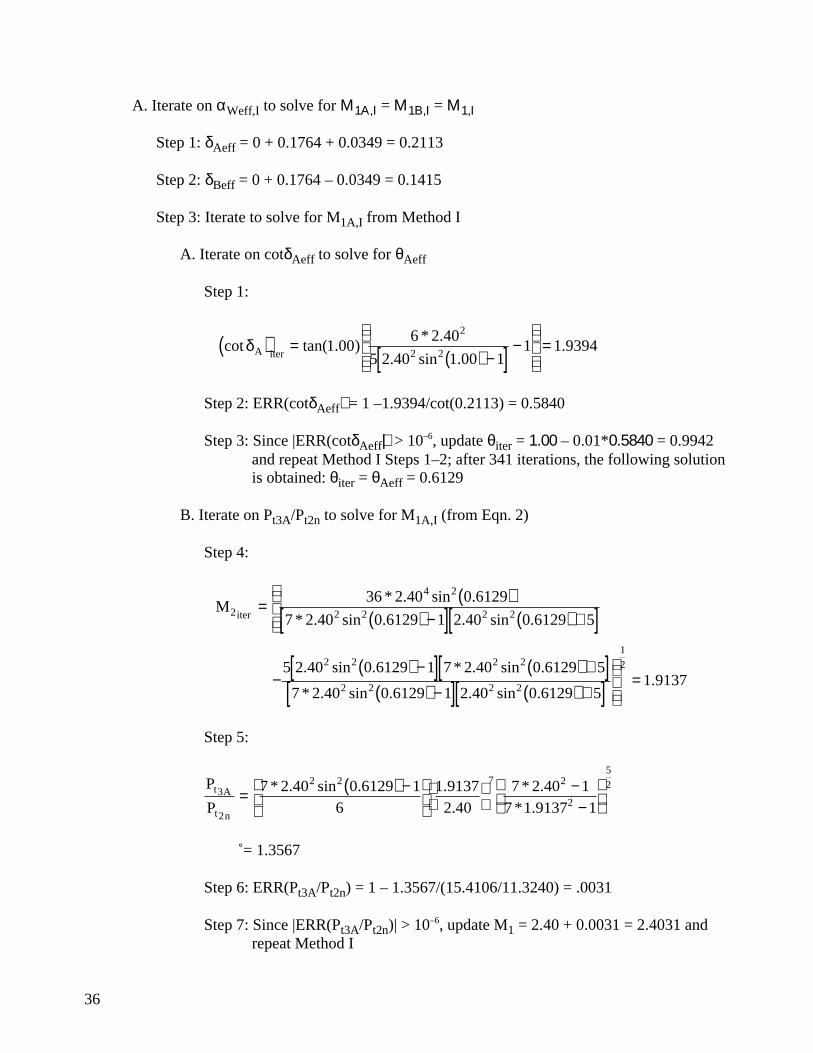
36

A. Iterate on αWeff,I to solve for Μ1Α,Ι = Μ1Β,Ι = Μ1,Ι

Step 1: δAeff = 0 + 0.1764 + 0.0349 = 0.2113

Step 2: δBeff = 0 + 0.1764 – 0.0349 = 0.1415

Step 3: Iterate to solve for M1A,I from Method I

A. Iterate on cotδAeff to solve for θAeff

Step 1:

cot tan( . )* .

. sin ..δA iter( ) =

( ) −[ ] −

=1 00

6 2 40

5 2 40 1 00 11 1 9394

2

2 2

Step 2: ERR(cotδAeff) = 1 –1.9394/cot(0.2113) = 0.5840

Step 3: Since |ERR(cotδAeff)| > 10–6, update θiter = 1.00 – 0.01*0.5840 = 0.9942and repeat Method I Steps 1–2; after 341 iterations, the following solutionis obtained: θiter = θAeff = 0.6129

B. Iterate on Pt3A/Pt2n to solve for M1A,I (from Eqn. 2)

Step 4:

Miter2

4 2

2 2 2 2

36 2 40 0 6129

7 2 40 0 6129 1 2 40 0 6129 5= ( )

( ) −[ ] ( ) +[ ]

* . sin .

* . sin . . sin .

−( ) −[ ] ( ) +[ ]

( ) −[ ] ( ) +[ ]

=

5 2 40 0 6129 1 7 2 40 0 6129 5

7 2 40 0 6129 1 2 40 0 6129 51 9137

2 2 2 2

2 2 2 2

1

2. sin . * . sin .

* . sin . . sin ..

Step 5:

P

Pt A

t n

3

2

2 2 7 2

2

5

27 2 40 0 6129 16

1 91372 40

7 2 40 17 1 9137 1

= ( ) −

−−

* . sin . ..

* .* .

 = 1.3567

Step 6: ERR(Pt3A/Pt2n) = 1 – 1.3567/(15.4106/11.3240) = .0031

Step 7: Since |ERR(Pt3A/Pt2n)| > 10–6, update M1 = 2.40 + 0.0031 = 2.4031 andrepeat Method I

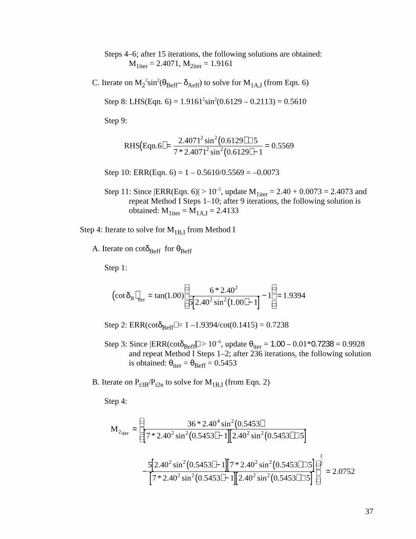
37

Steps 4–6; after 15 iterations, the following solutions are obtained:M1iter = 2.4071, M2iter = 1.9161

C. Iterate on M22sin2(θBeff– δAeff) to solve for M1A,I (from Eqn. 6)

Step 8: LHS(Eqn. 6) = 1.91612sin2(0.6129 – 0.2113) = 0.5610

Step 9:

RHS Eqn.. sin .

* . sin ..6

2 4071 0 6129 57 2 4071 0 6129 1

0 55692 2

2 2( ) = ( ) +( ) −

=

Step 10: ERR(Eqn. 6) = 1 – 0.5610/0.5569 = –0.0073

Step 11: Since |ERR(Eqn. 6)| > 10–5, update M1iter = 2.40 + 0.0073 = 2.4073 andrepeat Method I Steps 1–10; after 9 iterations, the following solution isobtained: M1iter = M1A,I = 2.4133

Step 4: Iterate to solve for M1B,I from Method I

A. Iterate on cotδBeff for θBeff

Step 1:

cot tan( . )* .

. sin ..δB iter( ) =

( ) −[ ] −

=1 00

6 2 40

5 2 40 1 00 11 1 9394

2

2 2

Step 2: ERR(cotδBeff) = 1 –1.9394/cot(0.1415) = 0.7238

Step 3: Since |ERR(cotδBeff)| > 10–6, update θiter = 1.00 – 0.01*0.7238 = 0.9928and repeat Method I Steps 1–2; after 236 iterations, the following solutionis obtained: θiter = θBeff = 0.5453

B. Iterate on Pt3B/Pt2n to solve for M1B,I (from Eqn. 2)

Step 4:

Miter2

4 2

2 2 2 2

36 2 40 0 5453

7 2 40 0 5453 1 2 40 0 5453 5= ( )

( ) −[ ] ( ) +[ ]

* . sin .

* . sin . . sin .

−( ) −[ ] ( ) +[ ]

( ) −[ ] ( ) +[ ]

=

5 2 40 0 5453 1 7 2 40 0 5453 5

7 2 40 0 5453 1 2 40 0 5453 52 0752

2 2 2 2

2 2 2 2

1

2. sin . * . sin .

* . sin . . sin ..

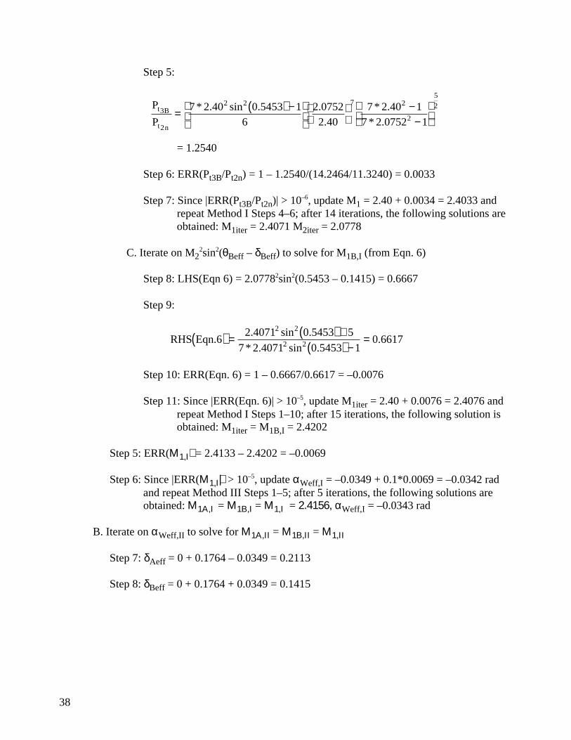
38

Step 5:

P

Pt B

t n

3

2

2 2 7 2

2

5

27 2 40 0 5453 16

2 07522 40

7 2 40 17 2 0752 1

= ( ) −

−−

* . sin . ..

* .* .

= 1.2540

Step 6: ERR(Pt3B/Pt2n) = 1 – 1.2540/(14.2464/11.3240) = 0.0033

Step 7: Since |ERR(Pt3B/Pt2n)| > 10–6, update M1 = 2.40 + 0.0034 = 2.4033 andrepeat Method I Steps 4–6; after 14 iterations, the following solutions areobtained: M1iter = 2.4071 M2iter = 2.0778

C. Iterate on M22sin2(θBeff – δBeff) to solve for M1B,I (from Eqn. 6)

Step 8: LHS(Eqn 6) = 2.07782sin2(0.5453 – 0.1415) = 0.6667

Step 9:

RHS Eqn.. sin .

* . sin ..6

2 4071 0 5453 57 2 4071 0 5453 1

0 66172 2

2 2( ) = ( ) +( ) −

=

Step 10: ERR(Eqn. 6) = 1 – 0.6667/0.6617 = –0.0076

Step 11: Since |ERR(Eqn. 6)| > 10–5, update M1iter = 2.40 + 0.0076 = 2.4076 andrepeat Method I Steps 1–10; after 15 iterations, the following solution isobtained: M1iter = M1B,I = 2.4202

Step 5: ERR(Μ1,Ι) = 2.4133 – 2.4202 = –0.0069

Step 6: Since |ERR(Μ1,Ι)| > 10–5, update αWeff,I = –0.0349 + 0.1*0.0069 = –0.0342 radand repeat Method III Steps 1–5; after 5 iterations, the following solutions areobtained: Μ1Α,Ι = Μ1Β,Ι = Μ1,Ι = 2.4156, αWeff,I = –0.0343 rad

B. Iterate on αWeff,II to solve for Μ1Α,ΙΙ = Μ1Β,ΙΙ = Μ1,ΙΙ

Step 7: δAeff = 0 + 0.1764 – 0.0349 = 0.2113

Step 8: δBeff = 0 + 0.1764 + 0.0349 = 0.1415

39

Step 9: Iterate for M1A,II from Method II

A. Iterate on cotδAeff to solve for θAeff

Step 1:

cot tan( . )* .

. sin ..δA iter( ) =

( ) −[ ] −

=1 00

6 2 40

5 2 40 1 00 11 1 9394

2

2 2

Step 2: ERR(cotδAeff) = 1 – 1.9394/cot(0.2113) = 0.5840

Step 3: Since |ERR(cotδAeff)| > 10–6, update θiter = 1.00 – 0.01*0.5840 = 0.9942and repeat Method I Steps 1–2; after 341 iterations, the following solutionis obtained: θiter = θAeff = 0.6129

B. Iterate on Pt2n/P2A to solve for Μ1Α,ΙΙ

Step 4:

P

Pt n

A

2

22 2

27

2

2

5

267 2 40 0 6129 1

6 2 405

67 2 40 1

=( ) −

−

* . sin .

* .* .

 = 3.8391

Step 5: ERR(Pt2n/P2A) = 3.8391 – 11.3240/3.0196 = 0.0890

Step 6: Since |ERR(Pt2n/P2A)| > 10–6, update M1iter = 2.40 – 0.1*0.0890 = 2.3911and repeat Method II Steps 1–5; after 38 iterations, the following solutionis obtained: M1iter = M1A,II = 2.3589

Step 10: Iterate to solve for M1B,II from Method II

A. Iterate on cotδBeff for θBeff

Step 1:

cot tan( . )* .

. sin ..δB iter( ) =

( ) −[ ] −

=1 00

6 2 40

5 2 40 1 00 11 1 9394

2

2 2

Step 2: ERR(cotδBeff) = 1 – 1.9394/cot(0.1415) = 0.7238

40

Step 3: Since |ERR(cotδBeff)| > 10–6, update θiter = 1.00 – 0.01*0.7238 = 0.9928and repeat Method I Steps 1–2; after 236 iterations, the following solutionis obtained: θiter = θBeff = 0.5453

B. Iterate on Pt2n/P2B to solve for Μ1Β,ΙΙ

Step 4:

P

Pt n

B

2

22 2

27

2

2

5

267 2 40 0 5453 1

6 2 405

67 2 40 1

=( ) −

−

* . sin .

* .* .

 = 4.8110

Step 5: ERR(Pt2n/P2B) = 4.8110 – 11.3240/2.3911 = 0.0751

Step 6: Since |ERR(Pt2n/P2B)| > 10–6, update M1 = 2.40 – 0.1*0.0751 = 2.3925and repeat Method II Steps 1–5; after 26 iterations, the following solutionis obtained: M1iter = M1B,II = 2.3750

Step 11: ERR(Μ1,ΙΙ) = 2.3589 – 2.3750 = –0.0161

Step 12: Since |ERR(Μ1,Ι)| > 10–5, update αWeff,II = –0.0349 – 0.1*0.0161 = –0.0365 radand repeat Method III Steps 7–12; after 3 iterations, the following solutions areobtained: Μ1Α,ΙΙ = Μ1Β,ΙΙ = Μ1,ΙΙ = 2.3671, αWeff,II = –0.0364 rad

C. Iterate on ∆δWeff to solve for Μ1,Ι = Μ1,ΙΙ = Μ1

Step 13: ERR(Μ1) = 2.4156 – 2.3671 = 0.0485

Step 14: Since |ERR(Μ1)| > 10–5, update ∆δWeff = 0 + 0.1*0.0485 = 0.0048 andrepeat Method III Steps 1–13; after 3 iterations, the following solutions areobtained: Μ1,Ι = Μ1,ΙΙ = Μ1 = 2.3916, ∆δWeff = 0.0046 rad = 0.261°,αWeff,I = –0.0359 rad = –2.057°, αWeff,II = –0.0364 rad = –2.086°

41

APPENDIX E

SAMPLE COMPRESSIBILITY PARAMETER CALCULATION

To demonstrate the calculation process for determining the cone-probe fundamentalcompressibility parameter, probe 4 on rake 1 will be analyzed. The following probe data areprovided for the computations:

Pt0 = 18.645 psia

PtY = 12.0886 psia

PA = 4.8990 psia

PB = 3.0313 psia

PC = 2.8279 psia

PD = 4.2387 psia

The compressibility parameter is computed from Eqn. 15:

PRT = + + + =4 8990 3 0313 2 8279 4 23874 12 0886

0 31014. . . .

* ..

The longitudinal and directional sensitivity parameters are computed from Eqn. 16:

PR

PR

AC

BD

= − =

= − = −

4 8990 2 827912 0886

0 17133

3 0313 4 238712 0886

0 099879

. ..

.

. ..

.

To calculate the fundamental compressibility parameter in Eqn. 21, the quadratic coefficients intable 2 (probe 4, rake 1) and an initial guess for PRT0 are required to initiate the iterativecomputations. For the first iteration cycle, PRT0 = 0.28000 is assumed:

PRACbiasT = 5.15935 – 36.2706*0.28000 + 63.2252*0.280002 = –0.0395623

PRBDbiasT = 0.10258 – 0.064912*0.28000 – 0.598695*0.280002 = 0.0374670

lT1 = 3.07195E+04 – 2.09517E+05*0.28000 + 3.56703E+05*0.280002 = 20.25520

lT2 = –6.77677E+08 + 4.76863E+09*0.28000 – 8.33091E+09*0.280002 = 4.39606E+06

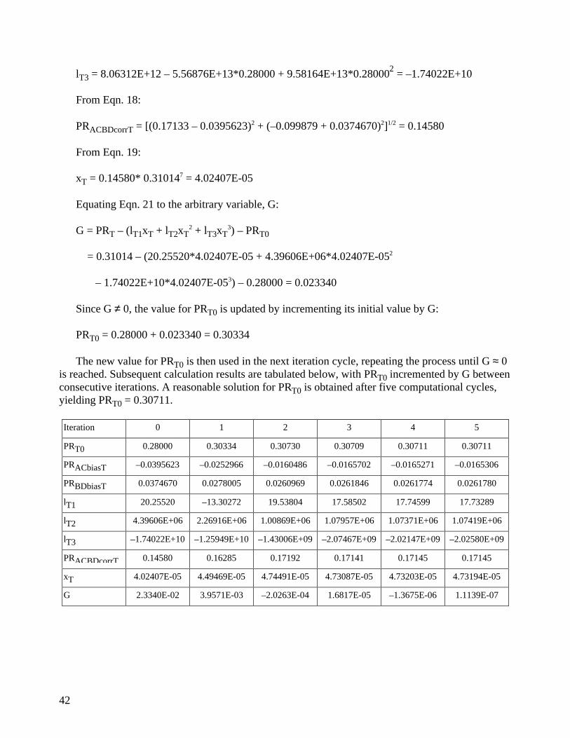
42

lT3 = 8.06312E+12 – 5.56876E+13*0.28000 + 9.58164E+13*0.280002 = –1.74022E+10

From Eqn. 18:

PRACBDcorrT = [(0.17133 – 0.0395623)2 + (–0.099879 + 0.0374670)2]1/2 = 0.14580

From Eqn. 19:

xT = 0.14580* 0.310147 = 4.02407E-05

Equating Eqn. 21 to the arbitrary variable, G:

G = PRT – (lT1xT + lT2xT2 + lT3xT

3) – PRT0

= 0.31014 – (20.25520*4.02407E-05 + 4.39606E+06*4.02407E-052

– 1.74022E+10*4.02407E-053) – 0.28000 = 0.023340

Since G ≠ 0, the value for PRT0 is updated by incrementing its initial value by G:

PRT0 = 0.28000 + 0.023340 = 0.30334

The new value for PRT0 is then used in the next iteration cycle, repeating the process until G ≈ 0is reached. Subsequent calculation results are tabulated below, with PRT0 incremented by G betweenconsecutive iterations. A reasonable solution for PRT0 is obtained after five computational cycles,yielding PRT0 = 0.30711.

Iteration 0 1 2 3 4 5

PRT0 0.28000 0.30334 0.30730 0.30709 0.30711 0.30711

PRACbiasT –0.0395623 –0.0252966 –0.0160486 –0.0165702 –0.0165271 –0.0165306

PRBDbiasT 0.0374670 0.0278005 0.0260969 0.0261846 0.0261774 0.0261780

lT1 20.25520 –13.30272 19.53804 17.58502 17.74599 17.73289

lT2 4.39606E+06 2.26916E+06 1.00869E+06 1.07957E+06 1.07371E+06 1.07419E+06

lT3 –1.74022E+10 –1.25949E+10 –1.43006E+09 –2.07467E+09 –2.02147E+09 –2.02580E+09

PRACBDcorrT 0.14580 0.16285 0.17192 0.17141 0.17145 0.17145

xT 4.02407E-05 4.49469E-05 4.74491E-05 4.73087E-05 4.73203E-05 4.73194E-05

G 2.3340E-02 3.9571E-03 –2.0263E-04 1.6817E-05 –1.3675E-06 1.1139E-07

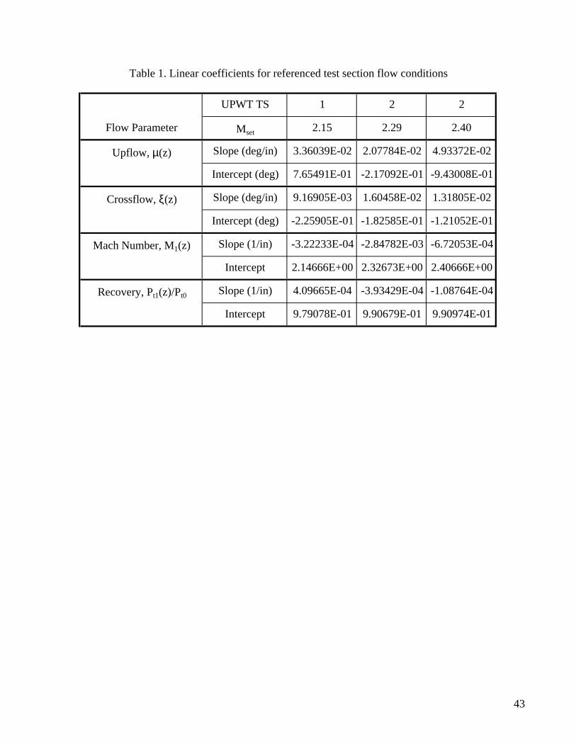
UPWT TS 1 2 2

Flow Parameter Mset 2.15 2.29 2.40

Upflow, µ(z) Slope (deg/in) 3.36039E-02 2.07784E-02 4.93372E-02

Intercept (deg) 7.65491E-01 -2.17092E-01 -9.43008E-01

Crossflow, ξ(z) Slope (deg/in) 9.16905E-03 1.60458E-02 1.31805E-02

Intercept (deg) -2.25905E-01 -1.82585E-01 -1.21052E-01

Mach Number, M1(z) Slope (1/in) -3.22233E-04 -2.84782E-03 -6.72053E-04

Intercept 2.14666E+00 2.32673E+00 2.40666E+00

Recovery, Pt1(z)/Pt0 Slope (1/in) 4.09665E-04 -3.93429E-04 -1.08764E-04

Intercept 9.79078E-01 9.90679E-01 9.90974E-01

Table 1. Linear coefficients for referenced test section flow conditions

43

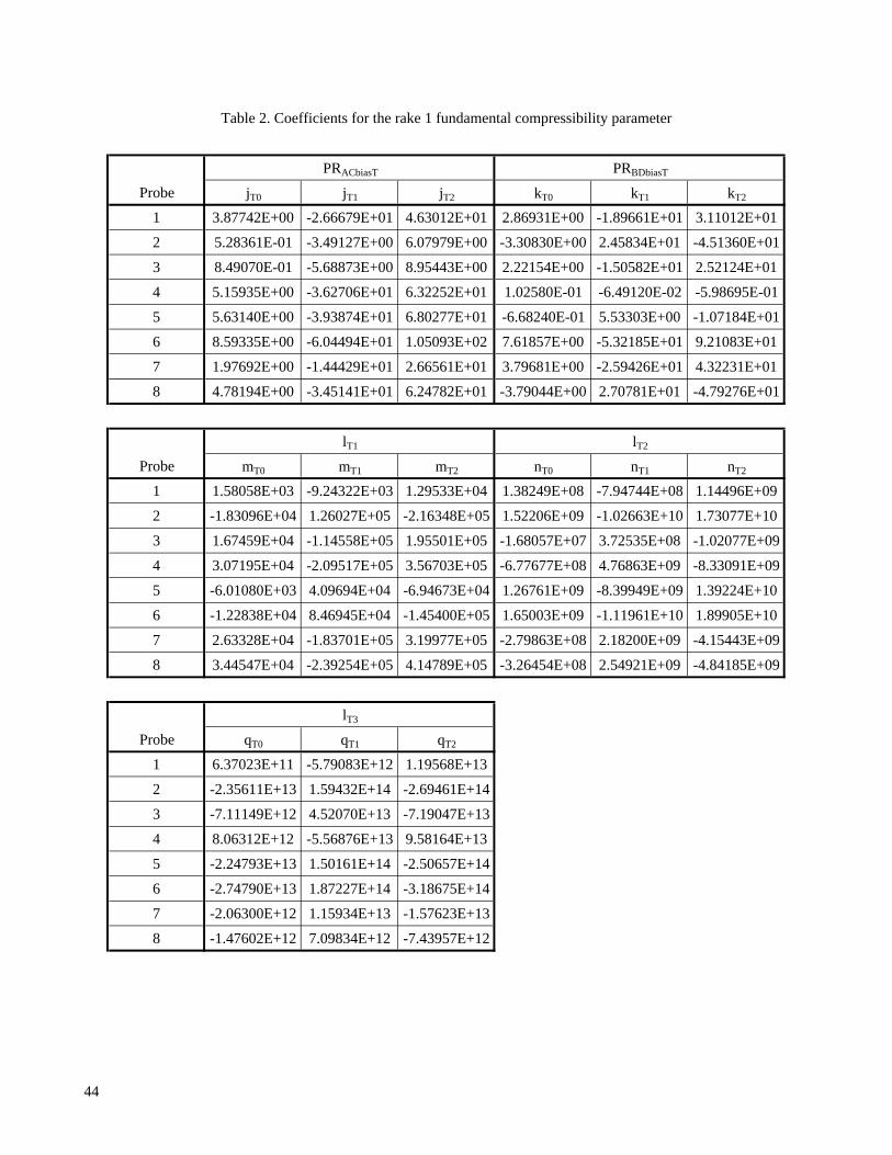
PRACbiasT PRBDbiasT

Probe jT0 jT1 jT2 kT0 kT1 kT2

1 3.87742E+00 -2.66679E+01 4.63012E+01 2.86931E+00 -1.89661E+01 3.11012E+01

2 5.28361E-01 -3.49127E+00 6.07979E+00 -3.30830E+00 2.45834E+01 -4.51360E+01

3 8.49070E-01 -5.68873E+00 8.95443E+00 2.22154E+00 -1.50582E+01 2.52124E+01

4 5.15935E+00 -3.62706E+01 6.32252E+01 1.02580E-01 -6.49120E-02 -5.98695E-01

5 5.63140E+00 -3.93874E+01 6.80277E+01 -6.68240E-01 5.53303E+00 -1.07184E+01

6 8.59335E+00 -6.04494E+01 1.05093E+02 7.61857E+00 -5.32185E+01 9.21083E+01

7 1.97692E+00 -1.44429E+01 2.66561E+01 3.79681E+00 -2.59426E+01 4.32231E+01

8 4.78194E+00 -3.45141E+01 6.24782E+01 -3.79044E+00 2.70781E+01 -4.79276E+01

lT1 lT2

Probe mT0 mT1 mT2 nT0 nT1 nT2

1 1.58058E+03 -9.24322E+03 1.29533E+04 1.38249E+08 -7.94744E+08 1.14496E+09

2 -1.83096E+04 1.26027E+05 -2.16348E+05 1.52206E+09 -1.02663E+10 1.73077E+10

3 1.67459E+04 -1.14558E+05 1.95501E+05 -1.68057E+07 3.72535E+08 -1.02077E+09

4 3.07195E+04 -2.09517E+05 3.56703E+05 -6.77677E+08 4.76863E+09 -8.33091E+09

5 -6.01080E+03 4.09694E+04 -6.94673E+04 1.26761E+09 -8.39949E+09 1.39224E+10

6 -1.22838E+04 8.46945E+04 -1.45400E+05 1.65003E+09 -1.11961E+10 1.89905E+10

7 2.63328E+04 -1.83701E+05 3.19977E+05 -2.79863E+08 2.18200E+09 -4.15443E+09

8 3.44547E+04 -2.39254E+05 4.14789E+05 -3.26454E+08 2.54921E+09 -4.84185E+09

lT3

Probe qT0 qT1 qT2

1 6.37023E+11 -5.79083E+12 1.19568E+13

2 -2.35611E+13 1.59432E+14 -2.69461E+14

3 -7.11149E+12 4.52070E+13 -7.19047E+13

4 8.06312E+12 -5.56876E+13 9.58164E+13

5 -2.24793E+13 1.50161E+14 -2.50657E+14

6 -2.74790E+13 1.87227E+14 -3.18675E+14

7 -2.06300E+12 1.15934E+13 -1.57623E+13

8 -1.47602E+12 7.09834E+12 -7.43957E+12

Table 2. Coefficients for the rake 1 fundamental compressibility parameter

44

PRACbiasT PRBDbiasT

Probe jT0 jT1 jT2 kT0 kT1 kT2

1 9.93132E+00 -7.02481E+01 1.25008E+02 1.11886E+00 -7.90968E+00 1.44470E+01

2 9.00664E-01 -5.68633E+00 8.77864E+00 -2.09080E+00 1.36876E+01 -2.14667E+01

3 1.82968E+00 -1.18867E+01 1.81672E+01 2.64358E+00 -1.91381E+01 3.52681E+01

4 8.45330E-01 -5.51382E+00 8.62861E+00 -3.58330E+00 2.43530E+01 -4.07843E+01

5 3.19486E-01 -2.03997E+00 3.04712E+00 1.33559E+00 -9.54829E+00 1.73636E+01

6 3.21875E-01 -2.01510E+00 3.12523E+00 -4.91985E+00 3.47691E+01 -6.14264E+01

lT1 lT2

Probe mT0 mT1 mT2 nT0 nT1 nT2

1 2.06233E+04 -1.46753E+05 2.60069E+05 -3.18328E+08 2.56042E+09 -4.98197E+09

2 -4.70170E+03 3.00921E+04 -4.80485E+04 5.16231E+08 -3.26680E+09 5.17226E+09

3 1.53285E+03 -1.01725E+04 1.70501E+04 6.25352E+08 -4.15146E+09 6.89531E+09

4 9.64282E+03 -6.57495E+04 1.11863E+05 2.88196E+08 -1.74190E+09 2.62960E+09

5 2.69995E+04 -1.85611E+05 3.18400E+05 -2.36035E+08 1.91786E+09 -3.73149E+09

6 5.19332E+02 -3.03113E+03 4.38688E+03 9.65690E+08 -6.38848E+09 1.05800E+10

lT3

Probe qT0 qT1 qT2

1 5.75679E+10 -4.22371E+12 1.33308E+13

2 -7.26511E+12 4.67084E+13 -7.50726E+13

3 -1.05745E+13 7.12439E+13 -1.19932E+14

4 -6.39594E+12 4.09404E+13 -6.55337E+13

5 -5.84456E+12 3.56734E+13 -5.42728E+13

6 -1.74805E+13 1.16582E+14 -1.94380E+14

Table 3. Coefficients for the rake 2 fundamental compressibility parameter

45

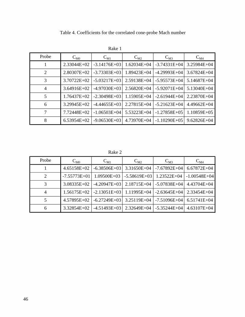
Rake 1

Probe CM0 CM1 CM2 CM3 CM4

1 2.33044E+02 -3.14176E+03 1.62034E+04 -3.74331E+04 3.25984E+04

2 2.80307E+02 -3.73303E+03 1.89423E+04 -4.29993E+04 3.67824E+04

3 3.70722E+02 -5.03217E+03 2.59138E+04 -5.95573E+04 5.14687E+04

4 3.64916E+02 -4.97030E+03 2.56820E+04 -5.92071E+04 5.13040E+04

5 1.76437E+02 -2.30498E+03 1.15905E+04 -2.61944E+04 2.23870E+04

6 3.29945E+02 -4.44655E+03 2.27815E+04 -5.21623E+04 4.49662E+04

7 7.72448E+02 -1.06503E+04 5.53223E+04 -1.27858E+05 1.10859E+05

8 6.53954E+02 -9.06530E+03 4.73970E+04 -1.10290E+05 9.62826E+04

Rake 2

Probe CM0 CM1 CM2 CM3 CM4

1 4.65158E+02 -6.38506E+03 3.31650E+04 -7.67892E+04 6.67872E+04

2 -7.55773E+01 1.09500E+03 -5.58619E+03 1.23522E+04 -1.00548E+04

3 3.08335E+02 -4.20947E+03 2.18715E+04 -5.07838E+04 4.43704E+04

4 1.56175E+02 -2.13051E+03 1.11995E+04 -2.63645E+04 2.33454E+04

5 4.57895E+02 -6.27249E+03 3.25119E+04 -7.51096E+04 6.51741E+04

6 3.32854E+02 -4.51493E+03 2.32649E+04 -5.35244E+04 4.63107E+04

Table 4. Coefficients for the correlated cone-probe Mach number

46

PRACbiasY PRBDbiasY

Probe jY0 jY1 jY2 kY0 kY1 kY2

1 8.29654E+00 -5.45409E+01 9.02695E+01 7.04530E+00 -4.27674E+01 6.50728E+01

2 1.59908E+00 -1.30324E+01 2.63212E+01 -1.21605E+01 8.33190E+01 -1.42183E+02

3 -5.43298E+00 3.82491E+01 -6.67566E+01 -6.91918E+00 4.86581E+01 -8.45437E+01

4 -1.22145E+01 8.35608E+01 -1.43777E+02 2.80416E+00 -2.02750E+01 3.75520E+01

5 -1.03334E+01 7.32933E+01 -1.28354E+02 -4.72693E+00 3.27423E+01 -5.59399E+01

6 -8.72178E+00 6.12402E+01 -1.07246E+02 -2.26857E+00 1.28667E+01 -1.69234E+01

7 3.78072E+01 -2.54995E+02 4.29077E+02 7.12244E+01 -4.94571E+02 8.59493E+02

8 -1.41770E+01 9.95480E+01 -1.75158E+02 3.57808E+01 -2.47096E+02 4.27543E+02

lY0 lY1

Probe mY0 mY1 mY2 nY0 nY1 nY2

1 7.89082E-01 -5.24939E+00 8.72743E+00 -8.32726E+00 5.56242E+01 -9.28902E+01

2 1.65910E-01 -1.19790E+00 2.16107E+00 7.84932E-02 1.55938E+00 -6.42128E+00

3 -3.35901E-01 2.33696E+00 -4.05133E+00 1.58962E+01 -1.09923E+02 1.89773E+02

4 1.49569E-01 -1.06437E+00 1.89135E+00 -1.80404E+01 1.26471E+02 -2.20702E+02

5 -6.82582E-01 4.71575E+00 -8.11587E+00 2.41466E+01 -1.66767E+02 2.87483E+02

6 1.00458E+00 -6.92463E+00 1.19246E+01 -3.00658E+01 2.07259E+02 -3.56780E+02

7 3.52092E+00 -2.44043E+01 4.22494E+01 -4.24751E+01 2.97986E+02 -5.21706E+02

8 1.66867E+00 -1.14532E+01 1.96400E+01 -4.25231E+01 2.95437E+02 -5.12372E+02

lY2 lY3

Probe qY0 qY1 qY2 rY0 rY1 rY2

1 5.62939E+01 -3.88147E+02 6.68547E+02 -1.27378E+02 8.78309E+02 -1.50763E+03

2 4.27282E+01 -3.10965E+02 5.63794E+02 -1.66779E+02 1.18952E+03 -2.11200E+03

3 -4.56012E+01 3.10908E+02 -5.29136E+02 -1.27297E+01 1.03173E+02 -2.00380E+02

4 8.80715E+01 -6.18125E+02 1.07876E+03 -1.88754E+02 1.32376E+03 -2.30389E+03

5 -9.49885E+01 6.54664E+02 -1.12669E+03 9.91666E+01 -6.82282E+02 1.17691E+03

6 2.24289E+02 -1.54151E+03 2.64535E+03 -5.75457E+02 3.95735E+03 -6.79059E+03

7 1.41764E+02 -9.99892E+02 1.75922E+03 -2.23568E+02 1.58096E+03 -2.78707E+03

8 1.60641E+02 -1.12022E+03 1.94994E+03 -3.34916E+02 2.33956E+03 -4.07337E+03

Table 5. Coefficients for the rake 1 correlated pitot pressure

47

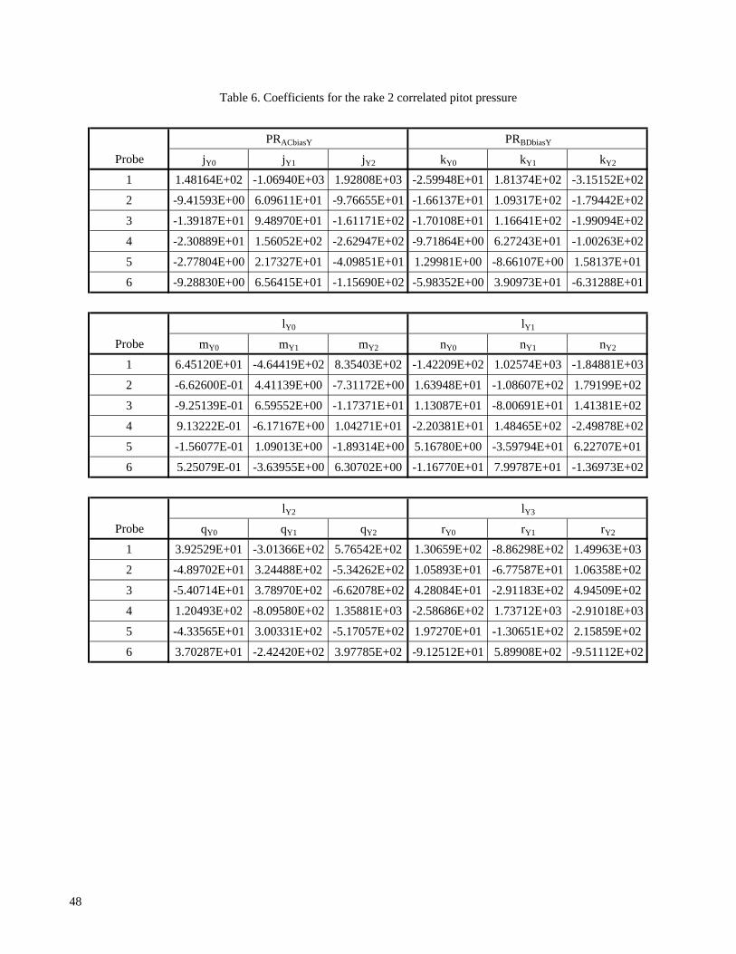
PRACbiasY PRBDbiasY

Probe jY0 jY1 jY2 kY0 kY1 kY2

1 1.48164E+02 -1.06940E+03 1.92808E+03 -2.59948E+01 1.81374E+02 -3.15152E+02

2 -9.41593E+00 6.09611E+01 -9.76655E+01 -1.66137E+01 1.09317E+02 -1.79442E+02

3 -1.39187E+01 9.48970E+01 -1.61171E+02 -1.70108E+01 1.16641E+02 -1.99094E+02

4 -2.30889E+01 1.56052E+02 -2.62947E+02 -9.71864E+00 6.27243E+01 -1.00263E+02

5 -2.77804E+00 2.17327E+01 -4.09851E+01 1.29981E+00 -8.66107E+00 1.58137E+01

6 -9.28830E+00 6.56415E+01 -1.15690E+02 -5.98352E+00 3.90973E+01 -6.31288E+01

lY0 lY1

Probe mY0 mY1 mY2 nY0 nY1 nY2

1 6.45120E+01 -4.64419E+02 8.35403E+02 -1.42209E+02 1.02574E+03 -1.84881E+03

2 -6.62600E-01 4.41139E+00 -7.31172E+00 1.63948E+01 -1.08607E+02 1.79199E+02

3 -9.25139E-01 6.59552E+00 -1.17371E+01 1.13087E+01 -8.00691E+01 1.41381E+02

4 9.13222E-01 -6.17167E+00 1.04271E+01 -2.20381E+01 1.48465E+02 -2.49878E+02

5 -1.56077E-01 1.09013E+00 -1.89314E+00 5.16780E+00 -3.59794E+01 6.22707E+01

6 5.25079E-01 -3.63955E+00 6.30702E+00 -1.16770E+01 7.99787E+01 -1.36973E+02

lY2 lY3

Probe qY0 qY1 qY2 rY0 rY1 rY2

1 3.92529E+01 -3.01366E+02 5.76542E+02 1.30659E+02 -8.86298E+02 1.49963E+03

2 -4.89702E+01 3.24488E+02 -5.34262E+02 1.05893E+01 -6.77587E+01 1.06358E+02

3 -5.40714E+01 3.78970E+02 -6.62078E+02 4.28084E+01 -2.91183E+02 4.94509E+02

4 1.20493E+02 -8.09580E+02 1.35881E+03 -2.58686E+02 1.73712E+03 -2.91018E+03

5 -4.33565E+01 3.00331E+02 -5.17057E+02 1.97270E+01 -1.30651E+02 2.15859E+02

6 3.70287E+01 -2.42420E+02 3.97785E+02 -9.12512E+01 5.89908E+02 -9.51112E+02

Table 6. Coefficients for the rake 2 correlated pitot pressure

48

Probe 1 C0 C1 C2 Probe 2 C0 C1 C2

a0 1.77666E+01 -1.27017E+02 2.13958E+02 a0 4.92881E+00 -3.10856E+01 4.82542E+01

a1 2.03862E+01 -4.44310E+02 7.28966E+02 a1 6.24949E+00 -3.51916E+02 5.66447E+02

c00 -1.80236E+01 1.23121E+02 -2.09761E+02 c00 -1.80307E+01 1.23958E+02 -2.13009E+02

c10 -2.23746E+02 1.56540E+03 -2.73145E+03 c10 -1.40085E+02 9.89622E+02 -1.76858E+03

c20 3.50499E+02 -2.68406E+03 5.02561E+03 c20 -7.37202E+02 5.23368E+03 -9.27270E+03

c30 5.88464E+03 -4.08997E+04 7.06051E+04 c30 2.93661E+03 -2.31363E+04 4.47240E+04

c40 -1.48943E+04 1.15675E+05 -2.21037E+05 c40 1.64032E+04 -1.28149E+05 2.47034E+05

c50 -6.75822E+04 4.66124E+05 -7.96036E+05 c50 4.21365E+03 4.28775E+04 -1.99028E+05

c60 9.89295E+04 -8.59081E+05 1.79915E+06 c60 1.07150E+05 -3.61052E+05 -4.59045E+04

c01 1.37979E+02 -9.35945E+02 1.58122E+03 c01 2.35600E+01 -1.63770E+02 2.80435E+02

c11 -1.16870E+03 8.27007E+03 -1.45655E+04 c11 -2.77321E+03 1.95657E+04 -3.43961E+04

c21 -8.91116E+03 5.92819E+04 -9.79256E+04 c21 -8.20643E+03 5.87673E+04 -1.05562E+05

c31 4.26743E+04 -3.07735E+05 5.50323E+05 c31 1.83330E+05 -1.29780E+06 2.29031E+06

c41 8.89552E+05 -5.96651E+06 9.92746E+06 c41 6.96398E+05 -5.00107E+06 8.95847E+06

c51 -7.02198E+05 5.08103E+06 -9.08992E+06 c51 -4.57472E+06 3.23686E+07 -5.71079E+07

c61 -2.38645E+07 1.61317E+08 -2.71067E+08 c61 -2.07543E+07 1.47818E+08 -2.62544E+08

c02 2.94301E+03 -2.01408E+04 3.44069E+04 c02 2.47721E+03 -1.69893E+04 2.90669E+04

c12 4.76441E+03 -3.39408E+04 5.99015E+04 c12 -1.35873E+03 6.58621E+03 -6.53139E+03

c22 -1.28070E+05 8.93313E+05 -1.55456E+06 c22 6.63495E+04 -4.68075E+05 8.18727E+05

c32 -4.37405E+05 3.06056E+06 -5.33021E+06 c32 7.60885E+05 -4.92825E+06 7.91269E+06

c42 1.37338E+07 -9.45877E+07 1.62699E+08 c42 2.95438E+06 -1.90506E+07 3.06009E+07

c52 2.55397E+05 -2.29178E+06 4.91291E+06 c52 -4.47027E+07 3.01547E+08 -5.06415E+08

c62 -3.29480E+08 2.26809E+09 -3.90111E+09 c62 -2.26986E+08 1.53733E+09 -2.59500E+09

c03 -5.61745E+03 3.80117E+04 -6.40773E+04 c03 -1.93791E+03 1.34983E+04 -2.32278E+04

c13 4.21336E+04 -2.96838E+05 5.21599E+05 c13 1.14426E+05 -8.08601E+05 1.42435E+06

c23 6.06802E+05 -4.13191E+06 7.02285E+06 c23 5.65680E+05 -3.99968E+06 7.07936E+06

c33 -4.95795E+05 3.98167E+06 -7.77464E+06 c33 -7.42673E+06 5.29421E+07 -9.40647E+07

c43 -4.97491E+07 3.38620E+08 -5.74462E+08 c43 -2.84180E+07 2.03733E+08 -3.65328E+08

c53 -7.41551E+06 4.11259E+07 -5.56428E+07 c53 1.57095E+08 -1.12487E+09 2.00767E+09

c63 1.36403E+09 -9.33520E+09 1.59313E+10 c63 6.28965E+08 -4.52512E+09 8.13179E+09

c04 -6.90083E+04 4.72455E+05 -8.07905E+05 c04 -5.97979E+04 4.12294E+05 -7.10261E+05

c14 -8.99452E+04 6.52615E+05 -1.16858E+06 c14 -3.82670E+04 3.63582E+05 -8.00610E+05

c24 3.59187E+06 -2.47245E+07 4.24603E+07 c24 -3.54272E+06 2.47365E+07 -4.29083E+07

c34 1.63848E+07 -1.14463E+08 1.99334E+08 c34 -4.61202E+06 2.05271E+07 -1.49260E+07

c44 -4.36435E+08 2.99302E+09 -5.12349E+09 c44 1.24220E+08 -8.97330E+08 1.61012E+09

c54 -1.65595E+08 1.16822E+09 -2.06367E+09 c54 6.46557E+08 -4.21146E+09 6.78640E+09

c64 1.18345E+10 -8.14290E+10 1.39914E+11 c64 1.58626E+09 -1.00278E+10 1.56321E+10

d0 -6.11746E-01 4.17411E+00 -7.14425E+00 d0 -2.33342E-01 1.60568E+00 -2.73659E+00

d1 1.38218E+01 -9.76110E+01 1.70959E+02 d1 1.36628E+00 -1.23725E+01 2.34164E+01

d2 6.85118E+02 -4.69961E+03 8.05866E+03 d2 5.49594E+02 -3.82352E+03 6.63354E+03

d3 -4.16504E+03 2.91059E+04 -5.06277E+04 d3 -1.41941E+03 1.03315E+04 -1.84556E+04

d4 -7.33975E+04 5.04760E+05 -8.67154E+05 d4 -6.05968E+04 4.21683E+05 -7.31841E+05

d5 1.63255E+05 -1.13647E+06 1.97082E+06 d5 4.18487E+04 -3.03191E+05 5.39823E+05

d6 1.86989E+06 -1.28809E+07 2.21550E+07 d6 1.49014E+06 -1.03665E+07 1.79864E+07

Table 7. Coefficients for the rake 1 correlated angle of attack

49

Probe 3 C0 C1 C2 Probe 4 C0 C1 C2

a0 2.40616E+01 -1.62561E+02 2.82064E+02 a0 4.60723E+01 -3.27059E+02 5.76278E+02

a1 -1.62133E+01 -1.88688E+02 2.87581E+02 a1 1.04807E+02 -1.05124E+03 1.82733E+03

c00 -1.77943E+01 1.22844E+02 -2.11275E+02 c00 -2.35286E+00 1.54251E+01 -2.49765E+01

c10 -1.66414E+02 1.16696E+03 -2.04557E+03 c10 -2.75760E+02 1.93776E+03 -3.41983E+03

c20 2.95756E+02 -2.18844E+03 4.01091E+03 c20 -1.34128E+03 9.61964E+03 -1.72101E+04

c30 -5.06702E+03 3.59801E+04 -6.35026E+04 c30 9.88801E+03 -7.16123E+04 1.29205E+05

c40 -3.87503E+04 2.75555E+05 -4.88413E+05 c40 -2.73922E+04 1.75509E+05 -2.79086E+05

c50 2.24735E+05 -1.57956E+06 2.76266E+06 c50 -1.88342E+05 1.36989E+06 -2.48406E+06

c60 1.02648E+06 -7.21146E+06 1.26243E+07 c60 1.09932E+06 -7.35676E+06 1.22855E+07

c01 3.51911E+01 -2.28382E+02 3.64864E+02 c01 1.75930E+02 -1.20482E+03 2.05846E+03

c11 -8.82941E+02 6.24721E+03 -1.10142E+04 c11 -1.44556E+03 9.88745E+03 -1.68046E+04

c21 5.26398E+03 -3.80200E+04 6.87894E+04 c21 -1.63193E+04 1.16011E+05 -2.05587E+05

c31 3.78892E+04 -2.73099E+05 4.95764E+05 c31 1.22266E+05 -8.44474E+05 1.45021E+06

c41 -7.31654E+04 5.36780E+05 -1.02062E+06 c41 1.56112E+06 -1.09987E+07 1.92863E+07

c51 -6.41153E+05 4.63797E+06 -8.52639E+06 c51 -3.13406E+06 2.17251E+07 -3.74714E+07

c61 -1.54040E+06 1.04126E+07 -1.73159E+07 c61 -3.31608E+07 2.32287E+08 -4.04933E+08

c02 1.37332E+03 -9.26976E+03 1.55041E+04 c02 -4.19018E+02 2.95615E+03 -5.23604E+03

c12 -5.10161E+03 3.64513E+04 -6.44092E+04 c12 1.33935E+04 -9.52366E+04 1.68386E+05

c22 2.05882E+04 -1.56305E+05 3.17598E+05 c22 7.74140E+04 -5.57065E+05 1.00017E+06

c32 2.24408E+06 -1.54936E+07 2.66078E+07 c32 -3.61805E+05 2.80415E+06 -5.33423E+06

c42 5.52846E+06 -3.59783E+07 5.67980E+07 c42 1.25573E+07 -8.43002E+07 1.40795E+08

c52 -8.40884E+07 5.77919E+08 -9.88497E+08 c52 -5.36242E+06 3.03487E+07 -4.10328E+07

c62 -2.69020E+08 1.80021E+09 -2.97706E+09 c62 -3.66859E+08 2.47902E+09 -4.17005E+09

c03 -2.61744E+03 1.73821E+04 -2.85857E+04 c03 -7.33012E+03 4.99560E+04 -8.49184E+04

c13 5.04598E+04 -3.57983E+05 6.34947E+05 c13 4.22705E+04 -2.86550E+05 4.82979E+05

c23 5.18790E+04 -3.26261E+05 5.24654E+05 c23 1.00608E+06 -7.12772E+06 1.26289E+07

c33 -9.62450E+05 8.14313E+06 -1.68705E+07 c33 -2.92067E+06 1.98599E+07 -3.35394E+07

c43 -5.47555E+06 4.18329E+07 -7.99687E+07 c43 -9.69705E+07 6.86382E+08 -1.21336E+09

c53 -2.88412E+07 1.58137E+08 -1.94424E+08 c53 6.91275E+07 -4.71859E+08 8.00373E+08

c63 1.77077E+07 -2.78879E+08 7.77239E+08 c63 2.13801E+09 -1.51063E+10 2.66454E+10

c04 -1.24841E+04 7.91567E+04 -1.21263E+05 c04 3.14622E+04 -2.18402E+05 3.79040E+05

c14 3.63743E+04 -2.72387E+05 4.95024E+05 c14 -3.80609E+05 2.69541E+06 -4.74589E+06

c24 -1.60696E+06 1.22151E+07 -2.37015E+07 c24 -6.62074E+06 4.69363E+07 -8.31111E+07

c34 -5.06365E+07 3.46802E+08 -5.90607E+08 c34 8.57637E+06 -6.55874E+07 1.23311E+08

c44 -5.47017E+07 2.73226E+08 -2.50579E+08 c44 2.91206E+07 -3.26149E+08 7.94493E+08

c54 2.13173E+09 -1.45731E+10 2.47948E+10 c54 1.84039E+08 -1.14444E+09 1.76215E+09

c64 5.77290E+09 -3.75432E+10 5.99926E+10 c64 2.66056E+09 -1.55474E+10 2.15160E+10

d0 -2.07822E+00 1.43284E+01 -2.47548E+01 d0 2.33744E-01 -1.70173E+00 3.01406E+00

d1 3.51513E+01 -2.40175E+02 4.09042E+02 d1 5.32156E+01 -3.56920E+02 5.95785E+02

d2 1.27592E+03 -8.82447E+03 1.52874E+04 d2 -6.39189E+01 5.38696E+02 -1.06266E+03

d3 -5.12250E+03 3.50433E+04 -5.97414E+04 d3 -9.12914E+03 6.17639E+04 -1.04314E+05

d4 -9.73421E+04 6.74830E+05 -1.17221E+06 d4 8.09710E+03 -6.58580E+04 1.27869E+05

d5 1.30090E+05 -8.86938E+05 1.50571E+06 d5 2.31528E+05 -1.56530E+06 2.64244E+06

d6 1.69062E+06 -1.17727E+07 2.05578E+07 d6 -2.34213E+05 1.84738E+06 -3.52173E+06

Table 7. Continued

50

Probe 5 C0 C1 C2 Probe 6 C0 C1 C2

a0 5.21393E+01 -3.73823E+02 6.58351E+02 a0 1.12967E+00 -3.41928E+00 -1.12070E+00

a1 6.90299E+01 -8.09177E+02 1.40907E+03 a1 -3.10679E+01 -9.40324E+01 1.24684E+02

c00 3.90641E+00 -2.72675E+01 4.79400E+01 c00 1.04475E+01 -7.37995E+01 1.30516E+02

c10 -1.04965E+02 7.06064E+02 -1.21584E+03 c10 -1.28509E+02 8.84337E+02 -1.53905E+03

c20 1.17570E+03 -8.07005E+03 1.38199E+04 c20 2.31311E+02 -1.52176E+03 2.49579E+03

c30 1.47589E+03 -1.12548E+04 2.11142E+04 c30 -4.23629E+03 3.07940E+04 -5.63294E+04

c40 -1.01300E+05 6.94459E+05 -1.18914E+06 c40 -4.51875E+04 3.03154E+05 -5.05074E+05

c50 2.27302E+03 3.56191E+03 -3.94981E+04 c50 1.15887E+05 -8.51685E+05 1.57007E+06

c60 1.90067E+06 -1.30130E+07 2.22564E+07 c60 8.24152E+05 -5.42402E+06 8.82741E+06

c01 1.40312E+02 -9.73923E+02 1.68236E+03 c01 1.54162E+02 -1.07225E+03 1.85628E+03

c11 6.41802E+02 -4.37684E+03 7.41659E+03 c11 -1.33014E+03 9.41222E+03 -1.65439E+04

c21 -8.88324E+03 6.08777E+04 -1.03639E+05 c21 2.02791E+03 -1.40022E+04 2.39016E+04

c31 3.07388E+04 -2.24921E+05 4.05413E+05 c31 8.07696E+04 -5.73653E+05 1.01347E+06

c41 1.10778E+06 -7.60309E+06 1.29639E+07 c41 8.47703E+05 -5.94274E+06 1.03595E+07

c51 -1.28814E+06 9.18874E+06 -1.62348E+07 c51 -1.40955E+06 1.00861E+07 -1.79695E+07

c61 -2.01712E+07 1.38176E+08 -2.35213E+08 c61 -2.52494E+07 1.76512E+08 -3.06993E+08

c02 -1.15293E+03 7.90591E+03 -1.35694E+04 c02 -2.43772E+03 1.69635E+04 -2.94960E+04

c12 -1.03083E+03 7.78127E+03 -1.42099E+04 c12 1.97871E+04 -1.38242E+05 2.40167E+05

c22 -2.32995E+05 1.58885E+06 -2.68901E+06 c22 -1.64840E+05 1.13567E+06 -1.94069E+06

c32 1.18765E+06 -8.23240E+06 1.41944E+07 c32 -6.23183E+05 4.24347E+06 -7.11748E+06

c42 2.05327E+07 -1.39303E+08 2.34948E+08 c42 3.46673E+07 -2.40748E+08 4.16129E+08

c52 -3.01604E+07 2.09064E+08 -3.60547E+08 c52 6.56606E+06 -4.16364E+07 6.29136E+07

c62 -3.66761E+08 2.47881E+09 -4.16507E+09 c62 -8.07504E+08 5.60836E+09 -9.69523E+09

c03 -4.82911E+03 3.36012E+04 -5.81334E+04 c03 -8.23595E+03 5.71597E+04 -9.87631E+04

c13 -3.12940E+04 2.07220E+05 -3.42689E+05 c13 2.29243E+04 -1.59624E+05 2.76703E+05

c23 7.08002E+05 -4.91357E+06 8.51482E+06 c23 1.66722E+05 -1.19951E+06 2.16863E+06

c33 -7.43167E+05 6.13338E+06 -1.20848E+07 c33 -1.47945E+06 1.03505E+07 -1.80391E+07

c43 -6.15370E+07 4.25583E+08 -7.34662E+08 c43 -5.15618E+07 3.64986E+08 -6.44270E+08

c53 4.63652E+07 -3.42452E+08 6.23053E+08 c53 1.49828E+07 -1.06998E+08 1.91257E+08

c63 1.06380E+09 -7.34144E+09 1.26468E+10 c63 1.34824E+09 -9.51025E+09 1.67160E+10

c04 4.37709E+04 -2.99987E+05 5.13641E+05 c04 9.07303E+04 -6.29165E+05 1.08961E+06

c14 8.14003E+03 -9.13272E+04 2.05205E+05 c14 -7.83047E+05 5.49300E+06 -9.59420E+06

c24 5.66748E+06 -3.80607E+07 6.35140E+07 c24 5.14971E+06 -3.58357E+07 6.19319E+07

c34 -3.01645E+07 2.10386E+08 -3.64397E+08 c34 4.20032E+07 -2.92843E+08 5.07410E+08

c44 -5.12335E+08 3.44046E+09 -5.75132E+09 c44 -1.11418E+09 7.77643E+09 -1.35181E+10

c54 8.37626E+08 -5.82982E+09 1.00842E+10 c54 -7.66549E+08 5.29498E+09 -9.07228E+09

c64 9.06144E+09 -6.06238E+10 1.00978E+11 c64 2.68387E+10 -1.87297E+11 3.25570E+11

d0 2.41914E+00 -1.66486E+01 2.85744E+01 d0 6.04736E-01 -4.26782E+00 7.52081E+00

d1 4.58615E+01 -3.13708E+02 5.34432E+02 d1 4.96666E+01 -3.39431E+02 5.77565E+02

d2 -9.67660E+02 6.64818E+03 -1.14100E+04 d2 -4.94999E+01 3.80141E+02 -7.27714E+02

d3 -7.07077E+03 4.82274E+04 -8.22129E+04 d3 -8.68325E+03 5.94970E+04 -1.01766E+05

d4 6.74319E+04 -4.64253E+05 7.98178E+05 d4 4.74720E+03 -3.42602E+04 6.22346E+04

d5 1.81140E+05 -1.23213E+06 2.09516E+06 d5 2.41833E+05 -1.65413E+06 2.82444E+06

d6 -1.19557E+06 8.25249E+06 -1.42230E+07 d6 -2.86378E+05 1.99239E+06 -3.47539E+06

Table 7. Continued

51

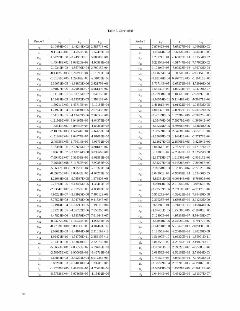
Probe 7 C0 C1 C2 Probe 8 C0 C1 C2

a0 2.10456E+01 -1.46244E+02 2.58571E+02 a0 7.97842E+01 -5.65377E+02 1.00925E+03

a1 -9.11643E+01 3.35856E+02 -6.52497E+02 a1 -3.16444E+02 1.96568E+03 -3.58031E+03

c00 4.52289E+00 -3.24961E+01 5.80080E+01 c00 1.23771E+01 -8.65075E+01 1.51564E+02

c10 -1.45448E+02 1.03820E+03 -1.90563E+03 c10 6.22554E+01 -4.51747E+02 7.77662E+02

c20 2.19345E+03 -1.56776E+04 2.79915E+04 c20 1.17204E+03 -8.07828E+03 1.39742E+04

c30 -8.43125E+03 5.76295E+04 -9.78710E+04 c30 -2.11635E+04 1.50550E+05 -2.67154E+05

c40 -1.81859E+05 1.29689E+06 -2.31038E+06 c40 -8.93176E+04 6.26477E+05 -1.10416E+06

c50 2.39071E+05 -1.64803E+06 2.82179E+06 c50 3.70714E+05 -2.65271E+06 4.72910E+06

c60 3.91827E+06 -2.79008E+07 4.96139E+07 c60 1.55030E+06 -1.09554E+07 1.94769E+07

c01 8.11130E+01 -5.83785E+02 1.04615E+03 c01 -2.77968E+00 1.18561E+01 -7.59392E+00

c11 1.18499E+03 -8.13372E+03 1.39913E+04 c11 -6.96554E+01 5.11446E+02 -9.30671E+02

c21 -1.69211E+03 1.43717E+04 -3.10188E+04 c21 1.46181E+04 -1.01422E+05 1.74583E+05

c31 1.71921E+04 -1.36060E+05 2.67643E+05 c31 4.04037E+04 -2.89956E+05 5.20722E+05

c41 5.51197E+05 -4.12497E+06 7.76653E+06 c41 -2.20139E+05 1.57596E+06 -2.78326E+06

c51 -1.21969E+06 8.94165E+06 -1.64376E+07 c51 -1.05470E+06 7.59279E+06 -1.36904E+07

c61 -1.32643E+07 9.88649E+07 -1.85362E+08 c61 -3.15225E+05 4.89466E+05 1.63668E+06

c02 -2.18076E+03 1.52844E+04 -2.67650E+04 c02 -2.93569E+03 2.04238E+04 -3.55319E+04

c12 -1.51266E+04 1.04877E+05 -1.81080E+05 c12 -1.19038E+03 1.14842E+04 -2.57176E+04

c22 -2.48758E+05 1.75614E+06 -3.09702E+06 c22 -3.11627E+05 2.18708E+06 -3.82594E+06

c32 3.18380E+06 -2.22635E+07 3.88189E+07 c32 1.06064E+06 -7.78226E+06 1.42167E+07

c42 3.09633E+07 -2.18236E+08 3.83966E+08 c42 3.18309E+07 -2.23828E+08 3.92525E+08

c52 -7.89492E+07 5.51859E+08 -9.61586E+08 c52 -2.18713E+07 1.61336E+08 -2.95817E+08

c62 -7.26656E+08 5.11757E+09 -8.99356E+09 c62 -6.31227E+08 4.44326E+09 -7.80096E+09

c03 -5.56069E+03 3.99320E+04 -7.13327E+04 c03 -2.09778E+03 1.52905E+04 -2.77625E+04

c13 -8.69975E+04 6.03446E+05 -1.04273E+06 c13 1.04200E+04 -7.96882E+04 1.52400E+05

c23 1.21039E+05 -9.78537E+05 1.97680E+06 c23 -5.89331E+05 4.00944E+06 -6.76300E+06

c33 2.72748E+05 -6.13455E+05 -1.35415E+06 c33 -3.06013E+06 2.21064E+07 -3.99560E+07

c43 -2.93647E+07 2.19259E+08 -4.09808E+08 c43 -2.22567E+06 2.07110E+07 -4.71473E+07

c53 4.95223E+07 -3.83925E+08 7.40612E+08 c53 5.95627E+07 -4.32628E+08 7.86439E+08

c63 6.77528E+08 -5.04788E+09 9.41324E+09 c63 2.30925E+08 -1.66081E+09 3.01242E+09

c04 9.71914E+04 -6.83211E+05 1.19911E+06 c04 9.65094E+04 -6.71810E+05 1.16844E+06

c14 6.29201E+05 -4.36752E+06 7.55626E+06 c14 -1.87451E+05 1.25830E+06 -2.10700E+06

c24 6.47825E+06 -4.53379E+07 7.91964E+07 c24 7.12800E+06 -4.95336E+07 8.56498E+07

c34 -8.83272E+07 6.14539E+08 -1.06593E+09 c34 -2.42058E+06 2.24824E+07 -4.79177E+07

c44 -8.27538E+08 5.80039E+09 -1.01467E+10 c44 -7.44730E+08 5.21267E+09 -9.09131E+09

c54 2.08662E+09 -1.44974E+10 2.51019E+10 c54 1.13056E+08 -9.20698E+08 1.80259E+09

c64 1.92421E+10 -1.34796E+11 2.35619E+11 c64 1.51490E+10 -1.06320E+11 1.85991E+11

d0 2.17391E+00 -1.53870E+01 2.72973E+01 d0 1.80358E+00 -1.25749E+01 2.19897E+01

d1 -5.66568E+01 4.03650E+02 -7.24606E+02 d1 -3.70341E+01 2.59022E+02 -4.55083E+02

d2 -2.58905E+02 1.90062E+03 -3.49718E+03 d2 2.08859E+02 -1.52163E+03 2.74024E+03

d3 4.67842E+03 -3.35294E+04 6.01238E+04 d3 5.75557E+03 -4.03657E+04 7.07063E+04

d4 8.83268E+03 -6.84088E+04 1.33281E+05 d4 -3.33222E+04 2.37091E+05 -4.19402E+05

d5 -1.32039E+05 9.49138E+05 -1.70639E+06 d5 -2.06513E+05 1.45528E+06 -2.56119E+06

d6 -5.57838E+04 5.07468E+05 -1.13402E+06 d6 1.04844E+06 -7.43420E+06 1.31307E+07

Table 7. Concluded

52

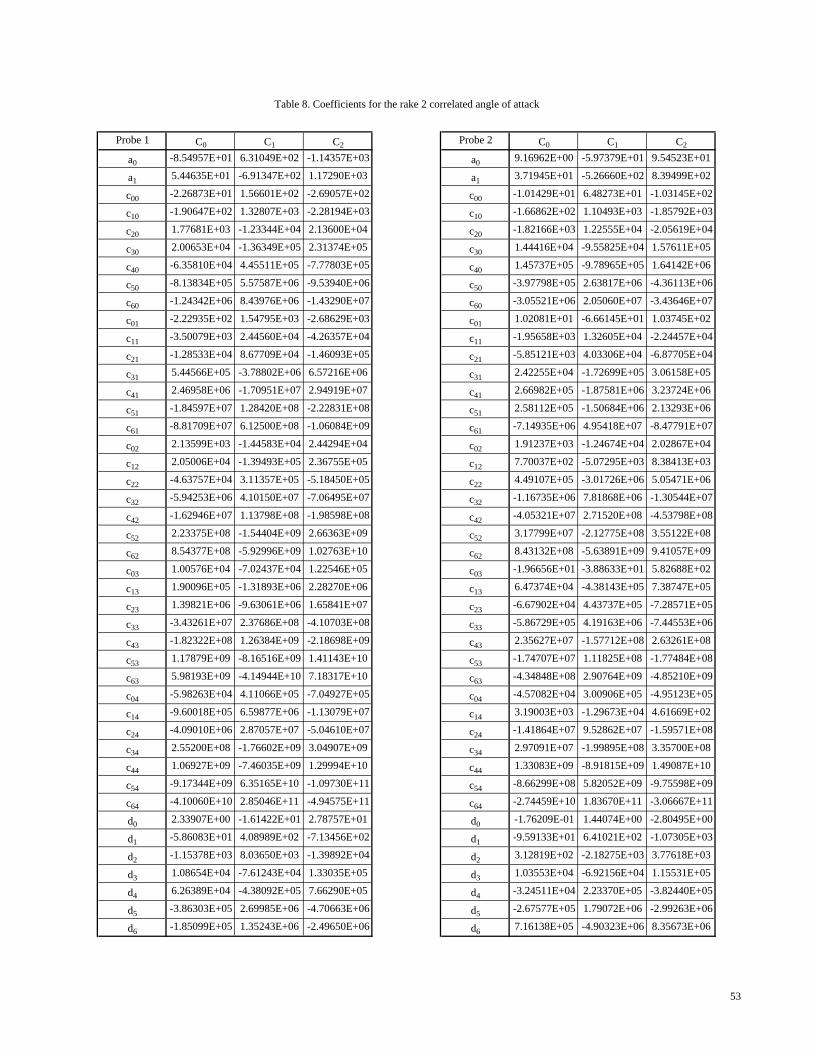
Probe 1 C0 C1 C2 Probe 2 C0 C1 C2

a0 -8.54957E+01 6.31049E+02 -1.14357E+03 a0 9.16962E+00 -5.97379E+01 9.54523E+01

a1 5.44635E+01 -6.91347E+02 1.17290E+03 a1 3.71945E+01 -5.26660E+02 8.39499E+02

c00 -2.26873E+01 1.56601E+02 -2.69057E+02 c00 -1.01429E+01 6.48273E+01 -1.03145E+02

c10 -1.90647E+02 1.32807E+03 -2.28194E+03 c10 -1.66862E+02 1.10493E+03 -1.85792E+03

c20 1.77681E+03 -1.23344E+04 2.13600E+04 c20 -1.82166E+03 1.22555E+04 -2.05619E+04

c30 2.00653E+04 -1.36349E+05 2.31374E+05 c30 1.44416E+04 -9.55825E+04 1.57611E+05

c40 -6.35810E+04 4.45511E+05 -7.77803E+05 c40 1.45737E+05 -9.78965E+05 1.64142E+06

c50 -8.13834E+05 5.57587E+06 -9.53940E+06 c50 -3.97798E+05 2.63817E+06 -4.36113E+06

c60 -1.24342E+06 8.43976E+06 -1.43290E+07 c60 -3.05521E+06 2.05060E+07 -3.43646E+07

c01 -2.22935E+02 1.54795E+03 -2.68629E+03 c01 1.02081E+01 -6.66145E+01 1.03745E+02

c11 -3.50079E+03 2.44560E+04 -4.26357E+04 c11 -1.95658E+03 1.32605E+04 -2.24457E+04

c21 -1.28533E+04 8.67709E+04 -1.46093E+05 c21 -5.85121E+03 4.03306E+04 -6.87705E+04

c31 5.44566E+05 -3.78802E+06 6.57216E+06 c31 2.42255E+04 -1.72699E+05 3.06158E+05

c41 2.46958E+06 -1.70951E+07 2.94919E+07 c41 2.66982E+05 -1.87581E+06 3.23724E+06

c51 -1.84597E+07 1.28420E+08 -2.22831E+08 c51 2.58112E+05 -1.50684E+06 2.13293E+06

c61 -8.81709E+07 6.12500E+08 -1.06084E+09 c61 -7.14935E+06 4.95418E+07 -8.47791E+07

c02 2.13599E+03 -1.44583E+04 2.44294E+04 c02 1.91237E+03 -1.24674E+04 2.02867E+04

c12 2.05006E+04 -1.39493E+05 2.36755E+05 c12 7.70037E+02 -5.07295E+03 8.38413E+03

c22 -4.63757E+04 3.11357E+05 -5.18450E+05 c22 4.49107E+05 -3.01726E+06 5.05471E+06

c32 -5.94253E+06 4.10150E+07 -7.06495E+07 c32 -1.16735E+06 7.81868E+06 -1.30544E+07

c42 -1.62946E+07 1.13798E+08 -1.98598E+08 c42 -4.05321E+07 2.71520E+08 -4.53798E+08

c52 2.23375E+08 -1.54404E+09 2.66363E+09 c52 3.17799E+07 -2.12775E+08 3.55122E+08

c62 8.54377E+08 -5.92996E+09 1.02763E+10 c62 8.43132E+08 -5.63891E+09 9.41057E+09

c03 1.00576E+04 -7.02437E+04 1.22546E+05 c03 -1.96656E+01 -3.88633E+01 5.82688E+02

c13 1.90096E+05 -1.31893E+06 2.28270E+06 c13 6.47374E+04 -4.38143E+05 7.38747E+05

c23 1.39821E+06 -9.63061E+06 1.65841E+07 c23 -6.67902E+04 4.43737E+05 -7.28571E+05

c33 -3.43261E+07 2.37686E+08 -4.10703E+08 c33 -5.86729E+05 4.19163E+06 -7.44553E+06

c43 -1.82322E+08 1.26384E+09 -2.18698E+09 c43 2.35627E+07 -1.57712E+08 2.63261E+08

c53 1.17879E+09 -8.16516E+09 1.41143E+10 c53 -1.74707E+07 1.11825E+08 -1.77484E+08

c63 5.98193E+09 -4.14944E+10 7.18317E+10 c63 -4.34848E+08 2.90764E+09 -4.85210E+09

c04 -5.98263E+04 4.11066E+05 -7.04927E+05 c04 -4.57082E+04 3.00906E+05 -4.95123E+05

c14 -9.60018E+05 6.59877E+06 -1.13079E+07 c14 3.19003E+03 -1.29673E+04 4.61669E+02

c24 -4.09010E+06 2.87057E+07 -5.04610E+07 c24 -1.41864E+07 9.52862E+07 -1.59571E+08

c34 2.55200E+08 -1.76602E+09 3.04907E+09 c34 2.97091E+07 -1.99895E+08 3.35700E+08

c44 1.06927E+09 -7.46035E+09 1.29994E+10 c44 1.33083E+09 -8.91815E+09 1.49087E+10

c54 -9.17344E+09 6.35165E+10 -1.09730E+11 c54 -8.66299E+08 5.82052E+09 -9.75598E+09

c64 -4.10060E+10 2.85046E+11 -4.94575E+11 c64 -2.74459E+10 1.83670E+11 -3.06667E+11

d0 2.33907E+00 -1.61422E+01 2.78757E+01 d0 -1.76209E-01 1.44074E+00 -2.80495E+00

d1 -5.86083E+01 4.08989E+02 -7.13456E+02 d1 -9.59133E+01 6.41021E+02 -1.07305E+03

d2 -1.15378E+03 8.03650E+03 -1.39892E+04 d2 3.12819E+02 -2.18275E+03 3.77618E+03

d3 1.08654E+04 -7.61243E+04 1.33035E+05 d3 1.03553E+04 -6.92156E+04 1.15531E+05

d4 6.26389E+04 -4.38092E+05 7.66290E+05 d4 -3.24511E+04 2.23370E+05 -3.82440E+05

d5 -3.86303E+05 2.69985E+06 -4.70663E+06 d5 -2.67577E+05 1.79072E+06 -2.99263E+06

d6 -1.85099E+05 1.35243E+06 -2.49650E+06 d6 7.16138E+05 -4.90323E+06 8.35673E+06

Table 8. Coefficients for the rake 2 correlated angle of attack

53

Probe 3 C0 C1 C2 Probe 4 C0 C1 C2

a0 3.19434E+01 -2.22542E+02 3.85438E+02 a0 2.04811E+01 -1.49536E+02 2.49857E+02

a1 -2.39431E+00 -2.89602E+02 4.68707E+02 a1 -1.47543E+01 -1.82111E+02 2.62818E+02

c00 -3.54604E-01 2.02814E+00 -2.77872E+00 c00 -2.05319E+00 1.07338E+01 -1.63340E+01

c10 -2.84907E+02 2.00401E+03 -3.49613E+03 c10 -3.02483E+02 2.00595E+03 -3.39597E+03

c20 -2.15942E+03 1.47031E+04 -2.50100E+04 c20 9.61942E+02 -6.33729E+03 1.04176E+04

c30 1.68061E+04 -1.15966E+05 1.99844E+05 c30 2.59979E+04 -1.73696E+05 2.89402E+05

c40 1.59150E+05 -1.08555E+06 1.85064E+06 c40 -1.28619E+04 8.39700E+04 -1.36579E+05

c50 -3.47429E+05 2.39443E+06 -4.11999E+06 c50 -1.26124E+06 8.43904E+06 -1.40886E+07

c60 -3.35694E+06 2.29646E+07 -3.92675E+07 c60 -3.61283E+06 2.42127E+07 -4.04887E+07

c01 1.46300E+02 -1.00458E+03 1.71766E+03 c01 8.10686E+01 -5.23050E+02 8.33744E+02

c11 4.09570E+02 -2.62109E+03 4.14175E+03 c11 2.17725E+03 -1.44192E+04 2.37382E+04

c21 9.53516E+03 -6.48419E+04 1.10122E+05 c21 8.54198E+03 -6.09196E+04 1.08385E+05

c31 -1.57045E+05 1.06995E+06 -1.81674E+06 c31 -2.59494E+05 1.68924E+06 -2.72894E+06

c41 4.00617E+04 -4.13944E+05 9.40096E+05 c41 -4.94138E+05 3.36451E+06 -5.72114E+06

c51 5.10757E+06 -3.50129E+07 5.98421E+07 c51 8.59557E+06 -5.55324E+07 8.89599E+07

c61 -1.01105E+07 7.27132E+07 -1.30199E+08 c61 2.80187E+07 -1.82414E+08 2.94984E+08

c02 -6.06841E+02 4.17341E+03 -7.19007E+03 c02 -4.17376E+02 2.79052E+03 -4.66137E+03

c12 1.20246E+04 -8.32096E+04 1.44015E+05 c12 3.14743E+04 -2.10284E+05 3.50038E+05

c22 5.84065E+05 -4.00309E+06 6.85154E+06 c22 -4.44635E+04 2.86392E+05 -4.61008E+05

c32 -1.28607E+05 8.71142E+05 -1.52839E+06 c32 -3.28359E+06 2.17228E+07 -3.57715E+07

c42 -4.86836E+07 3.34160E+08 -5.72420E+08 c42 -1.27759E+06 8.34199E+06 -1.32931E+07

c52 -2.13271E+07 1.47509E+08 -2.53139E+08 c52 1.54397E+08 -1.02270E+09 1.68773E+09

c62 1.10002E+09 -7.55690E+09 1.29531E+10 c62 4.90624E+08 -3.24836E+09 5.35586E+09

c03 -6.80005E+03 4.65739E+04 -7.93882E+04 c03 -4.25240E+03 2.78958E+04 -4.53863E+04

c13 -4.08112E+04 2.76058E+05 -4.64825E+05 c13 -1.53939E+05 1.02703E+06 -1.70725E+06

c23 -5.93303E+05 4.07409E+06 -6.97410E+06 c23 -1.02055E+05 8.26953E+05 -1.63600E+06

c33 9.14218E+06 -6.25710E+07 1.06734E+08 c33 2.22951E+07 -1.47837E+08 2.44319E+08

c43 2.58412E+07 -1.75645E+08 2.97219E+08 c43 3.26150E+07 -2.21480E+08 3.75915E+08

c53 -2.62934E+08 1.80278E+09 -3.08147E+09 c53 -7.88686E+08 5.21544E+09 -8.59579E+09

c63 -1.41173E+08 9.26217E+08 -1.50112E+09 c63 -2.56544E+09 1.70327E+10 -2.82037E+10

c04 2.29156E+04 -1.55051E+05 2.62257E+05 c04 3.61498E+03 -2.34469E+04 3.82852E+04

c14 -2.97956E+05 2.03964E+06 -3.49028E+06 c14 -1.12497E+06 7.52004E+06 -1.25294E+07

c24 -1.86418E+07 1.27983E+08 -2.19274E+08 c24 1.46092E+06 -9.21816E+06 1.44076E+07

c34 -2.59935E+06 1.97495E+07 -3.55038E+07 c34 1.49028E+08 -9.90270E+08 1.64033E+09

c44 1.61264E+09 -1.10841E+10 1.90019E+10 c44 1.09935E+08 -7.45160E+08 1.26010E+09

c54 9.04591E+08 -6.28030E+09 1.08325E+10 c54 -6.17674E+09 4.10255E+10 -6.79420E+10

c64 -3.62926E+10 2.49590E+11 -4.28055E+11 c64 -1.94793E+10 1.29599E+11 -2.15024E+11

d0 -8.62893E-01 5.93706E+00 -1.02134E+01 d0 1.45549E+00 -9.43688E+00 1.47732E+01

d1 3.66053E+01 -2.47902E+02 4.19234E+02 d1 -7.19318E+01 4.83173E+02 -8.21695E+02

d2 5.35623E+02 -3.67839E+03 6.31684E+03 d2 -6.81969E+02 4.53712E+03 -7.53430E+03

d3 -3.65234E+03 2.42847E+04 -4.04138E+04 d3 6.31764E+03 -4.31265E+04 7.33683E+04

d4 -4.23630E+04 2.90762E+05 -4.99328E+05 d4 4.37736E+04 -2.94342E+05 4.93960E+05

d5 9.19296E+04 -6.09292E+05 1.01128E+06 d5 -2.13046E+05 1.46089E+06 -2.49422E+06

d6 8.25171E+05 -5.66498E+06 9.73510E+06 d6 -1.09086E+06 7.42222E+06 -1.25887E+07

Table 8. Continued

54

Probe 5 C0 C1 C2 Probe 6 C0 C1 C2

a0 -6.46899E+00 4.44996E+01 -8.47579E+01 a0 9.28387E+00 -6.06612E+01 1.05057E+02

a1 -9.13391E+01 3.36424E+02 -6.41976E+02 a1 -3.91913E+01 -3.08247E+01 8.80932E+00

c00 -5.64650E-01 2.33763E+00 -4.04088E+00 c00 1.77255E+01 -1.23979E+02 2.16309E+02

c10 -1.52075E+02 1.03592E+03 -1.80956E+03 c10 -1.52900E+02 9.98181E+02 -1.70179E+03

c20 1.65698E+03 -1.13191E+04 1.93261E+04 c20 -2.18784E+03 1.50500E+04 -2.58616E+04

c30 1.71982E+04 -1.15841E+05 1.94695E+05 c30 1.23454E+04 -8.22339E+04 1.36214E+05

c40 -7.47923E+04 5.17362E+05 -8.94032E+05 c40 2.46934E+05 -1.69545E+06 2.90453E+06

c50 -1.13952E+06 7.75444E+06 -1.31759E+07 c50 -4.70011E+05 3.17153E+06 -5.33063E+06

c60 -2.65708E+06 1.80159E+07 -3.04981E+07 c60 -6.27698E+06 4.31141E+07 -7.38700E+07

c01 6.43833E+01 -4.52689E+02 7.90731E+02 c01 2.28307E+01 -1.60777E+02 2.81355E+02

c11 1.69289E+03 -1.16538E+04 2.00159E+04 c11 6.27430E+02 -4.22756E+03 7.15087E+03

c21 -5.19308E+03 3.43932E+04 -5.69242E+04 c21 1.75017E+04 -1.22700E+05 2.14350E+05

c31 -9.96130E+04 6.57276E+05 -1.07347E+06 c31 1.53518E+04 -1.13773E+05 2.11539E+05

c41 3.24917E+05 -2.23402E+06 3.82977E+06 c41 -1.08400E+03 2.19041E+05 -7.57307E+05

c51 5.26605E+06 -3.48257E+07 5.70854E+07 c51 -1.61320E+06 1.13390E+07 -1.99594E+07

c61 1.27234E+07 -8.33303E+07 1.35099E+08 c61 -1.41856E+07 9.28399E+07 -1.50845E+08

c02 -2.32528E+03 1.61159E+04 -2.78291E+04 c02 -3.12445E+03 2.15445E+04 -3.70946E+04

c12 1.34451E+04 -9.16974E+04 1.56143E+05 c12 1.52488E+04 -1.00724E+05 1.65826E+05

c22 -1.74162E+05 1.19743E+06 -2.05707E+06 c22 4.11795E+05 -2.81777E+06 4.80882E+06

c32 -4.20933E+06 2.86802E+07 -4.87218E+07 c32 -1.82203E+06 1.20745E+07 -1.99382E+07

c42 5.73659E+06 -4.03772E+07 7.10163E+07 c42 -4.23545E+07 2.88455E+08 -4.89693E+08

c52 2.64420E+08 -1.81052E+09 3.09222E+09 c52 6.14823E+07 -4.12422E+08 6.89866E+08

c62 7.73417E+08 -5.28755E+09 9.01588E+09 c62 1.08047E+09 -7.35559E+09 1.24819E+10

c03 -3.56413E+03 2.53869E+04 -4.49311E+04 c03 -1.54053E+03 1.06717E+04 -1.83857E+04

c13 -1.18244E+05 8.20251E+05 -1.42029E+06 c13 -5.28442E+04 3.67145E+05 -6.34947E+05

c23 4.62397E+05 -3.17633E+06 5.44777E+06 c23 -1.24116E+06 8.73608E+06 -1.53110E+07

c33 1.18827E+07 -8.16866E+07 1.40077E+08 c33 -2.25929E+06 1.51993E+07 -2.56503E+07

c43 -1.03766E+07 7.16911E+07 -1.23686E+08 c43 2.60493E+07 -1.96916E+08 3.67267E+08

c53 -5.21319E+08 3.57451E+09 -6.11394E+09 c53 1.28570E+08 -8.78081E+08 1.50033E+09

c63 -1.42787E+09 9.78150E+09 -1.67166E+10 c63 2.41257E+08 -1.26951E+09 1.52862E+09

c04 7.33078E+04 -5.06466E+05 8.71969E+05 c04 9.19683E+04 -6.31741E+05 1.08324E+06

c14 -4.05386E+05 2.77238E+06 -4.73209E+06 c14 -3.67365E+05 2.38901E+06 -3.86685E+06

c24 7.54806E+06 -5.20749E+07 8.97165E+07 c24 -9.60873E+06 6.52024E+07 -1.10379E+08

c34 1.53407E+08 -1.05091E+09 1.79507E+09 c34 6.70484E+07 -4.47198E+08 7.44039E+08

c44 -2.57221E+08 1.79858E+09 -3.14189E+09 c44 1.13933E+09 -7.71379E+09 1.30201E+10

c54 -9.35187E+09 6.42538E+10 -1.10107E+11 c54 -2.13979E+09 1.43954E+10 -2.41645E+10

c64 -2.65644E+10 1.82259E+11 -3.11848E+11 c64 -3.03713E+10 2.05874E+11 -3.47909E+11

d0 7.46026E-01 -4.90252E+00 8.00906E+00 d0 3.92899E+00 -2.65850E+01 4.51060E+01

d1 -8.42795E+01 5.87125E+02 -1.02685E+03 d1 -6.10299E+01 4.20077E+02 -7.33304E+02

d2 -1.04290E+02 6.71986E+02 -1.09965E+03 d2 -8.41850E+02 5.73028E+03 -9.75869E+03

d3 1.01090E+04 -7.07033E+04 1.23702E+05 d3 6.01242E+03 -4.19079E+04 7.26575E+04

d4 2.21960E+04 -1.51422E+05 2.60563E+05 d4 3.76582E+04 -2.55733E+05 4.36568E+05

d5 -3.09008E+05 2.16517E+06 -3.79520E+06 d5 -1.68045E+05 1.17150E+06 -2.02938E+06

d6 -9.43920E+05 6.54602E+06 -1.14018E+07 d6 -4.66813E+05 3.14688E+06 -5.36874E+06

Table 8. Concluded

55

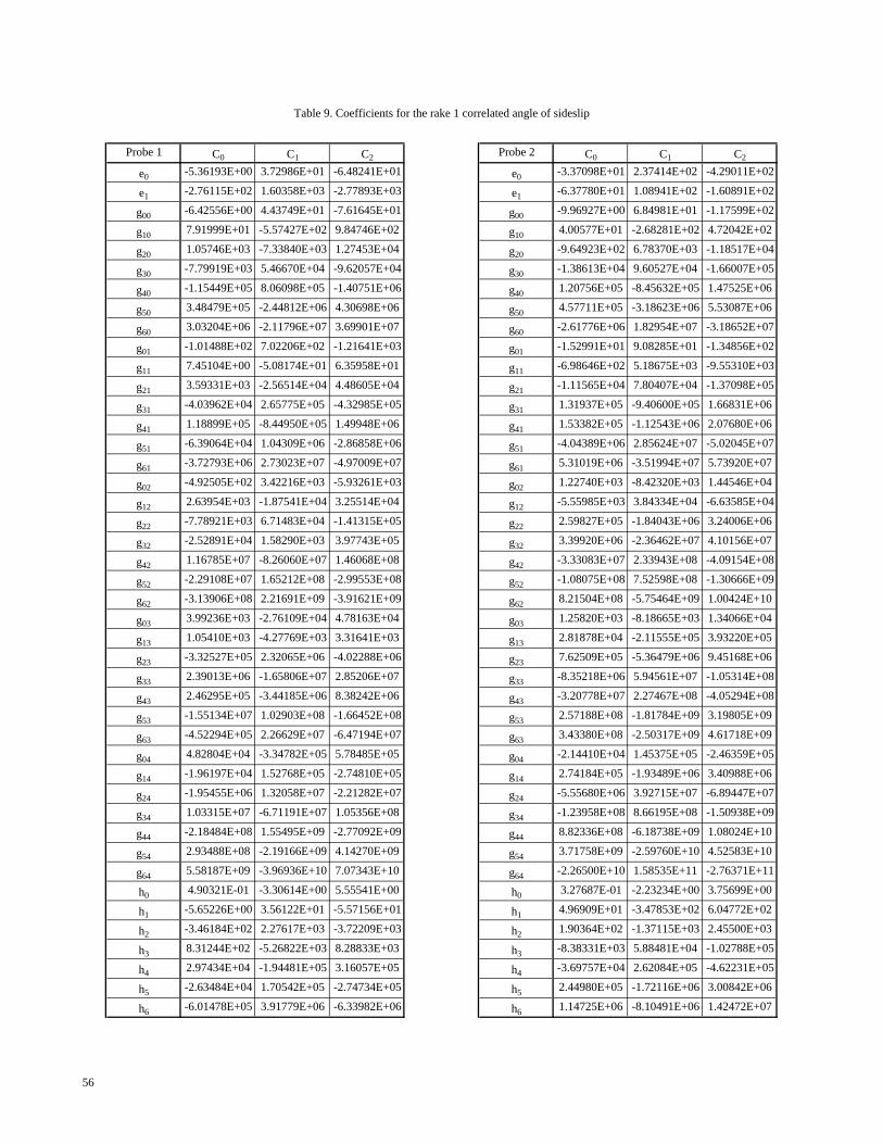
Probe 1 C0 C1 C2 Probe 2 C0 C1 C2

e0 -5.36193E+00 3.72986E+01 -6.48241E+01 e0 -3.37098E+01 2.37414E+02 -4.29011E+02

e1 -2.76115E+02 1.60358E+03 -2.77893E+03 e1 -6.37780E+01 1.08941E+02 -1.60891E+02

g00 -6.42556E+00 4.43749E+01 -7.61645E+01 g00 -9.96927E+00 6.84981E+01 -1.17599E+02

g10 7.91999E+01 -5.57427E+02 9.84746E+02 g10 4.00577E+01 -2.68281E+02 4.72042E+02

g20 1.05746E+03 -7.33840E+03 1.27453E+04 g20 -9.64923E+02 6.78370E+03 -1.18517E+04

g30 -7.79919E+03 5.46670E+04 -9.62057E+04 g30 -1.38613E+04 9.60527E+04 -1.66007E+05

g40 -1.15449E+05 8.06098E+05 -1.40751E+06 g40 1.20756E+05 -8.45632E+05 1.47525E+06

g50 3.48479E+05 -2.44812E+06 4.30698E+06 g50 4.57711E+05 -3.18623E+06 5.53087E+06

g60 3.03204E+06 -2.11796E+07 3.69901E+07 g60 -2.61776E+06 1.82954E+07 -3.18652E+07

g01 -1.01488E+02 7.02206E+02 -1.21641E+03 g01 -1.52991E+01 9.08285E+01 -1.34856E+02

g11 7.45104E+00 -5.08174E+01 6.35958E+01 g11 -6.98646E+02 5.18675E+03 -9.55310E+03

g21 3.59331E+03 -2.56514E+04 4.48605E+04 g21 -1.11565E+04 7.80407E+04 -1.37098E+05

g31 -4.03962E+04 2.65775E+05 -4.32985E+05 g31 1.31937E+05 -9.40600E+05 1.66831E+06

g41 1.18899E+05 -8.44950E+05 1.49948E+06 g41 1.53382E+05 -1.12543E+06 2.07680E+06

g51 -6.39064E+04 1.04309E+06 -2.86858E+06 g51 -4.04389E+06 2.85624E+07 -5.02045E+07

g61 -3.72793E+06 2.73023E+07 -4.97009E+07 g61 5.31019E+06 -3.51994E+07 5.73920E+07

g02 -4.92505E+02 3.42216E+03 -5.93261E+03 g02 1.22740E+03 -8.42320E+03 1.44546E+04

g12 2.63954E+03 -1.87541E+04 3.25514E+04 g12 -5.55985E+03 3.84334E+04 -6.63585E+04

g22 -7.78921E+03 6.71483E+04 -1.41315E+05 g22 2.59827E+05 -1.84043E+06 3.24006E+06

g32 -2.52891E+04 1.58290E+03 3.97743E+05 g32 3.39920E+06 -2.36462E+07 4.10156E+07

g42 1.16785E+07 -8.26060E+07 1.46068E+08 g42 -3.33083E+07 2.33943E+08 -4.09154E+08

g52 -2.29108E+07 1.65212E+08 -2.99553E+08 g52 -1.08075E+08 7.52598E+08 -1.30666E+09

g62 -3.13906E+08 2.21691E+09 -3.91621E+09 g62 8.21504E+08 -5.75464E+09 1.00424E+10

g03 3.99236E+03 -2.76109E+04 4.78163E+04 g03 1.25820E+03 -8.18665E+03 1.34066E+04

g13 1.05410E+03 -4.27769E+03 3.31641E+03 g13 2.81878E+04 -2.11555E+05 3.93220E+05

g23 -3.32527E+05 2.32065E+06 -4.02288E+06 g23 7.62509E+05 -5.36479E+06 9.45168E+06

g33 2.39013E+06 -1.65806E+07 2.85206E+07 g33 -8.35218E+06 5.94561E+07 -1.05314E+08

g43 2.46295E+05 -3.44185E+06 8.38242E+06 g43 -3.20778E+07 2.27467E+08 -4.05294E+08

g53 -1.55134E+07 1.02903E+08 -1.66452E+08 g53 2.57188E+08 -1.81784E+09 3.19805E+09

g63 -4.52294E+05 2.26629E+07 -6.47194E+07 g63 3.43380E+08 -2.50317E+09 4.61718E+09

g04 4.82804E+04 -3.34782E+05 5.78485E+05 g04 -2.14410E+04 1.45375E+05 -2.46359E+05

g14 -1.96197E+04 1.52768E+05 -2.74810E+05 g14 2.74184E+05 -1.93489E+06 3.40988E+06

g24 -1.95455E+06 1.32058E+07 -2.21282E+07 g24 -5.55680E+06 3.92715E+07 -6.89447E+07

g34 1.03315E+07 -6.71191E+07 1.05356E+08 g34 -1.23958E+08 8.66195E+08 -1.50938E+09

g44 -2.18484E+08 1.55495E+09 -2.77092E+09 g44 8.82336E+08 -6.18738E+09 1.08024E+10

g54 2.93488E+08 -2.19166E+09 4.14270E+09 g54 3.71758E+09 -2.59760E+10 4.52583E+10

g64 5.58187E+09 -3.96936E+10 7.07343E+10 g64 -2.26500E+10 1.58535E+11 -2.76371E+11

h0 4.90321E-01 -3.30614E+00 5.55541E+00 h0 3.27687E-01 -2.23234E+00 3.75699E+00

h1 -5.65226E+00 3.56122E+01 -5.57156E+01 h1 4.96909E+01 -3.47853E+02 6.04772E+02

h2 -3.46184E+02 2.27617E+03 -3.72209E+03 h2 1.90364E+02 -1.37115E+03 2.45500E+03

h3 8.31244E+02 -5.26822E+03 8.28833E+03 h3 -8.38331E+03 5.88481E+04 -1.02788E+05

h4 2.97434E+04 -1.94481E+05 3.16057E+05 h4 -3.69757E+04 2.62084E+05 -4.62231E+05

h5 -2.63484E+04 1.70542E+05 -2.74734E+05 h5 2.44980E+05 -1.72116E+06 3.00842E+06

h6 -6.01478E+05 3.91779E+06 -6.33982E+06 h6 1.14725E+06 -8.10491E+06 1.42472E+07

Table 9. Coefficients for the rake 1 correlated angle of sideslip

56

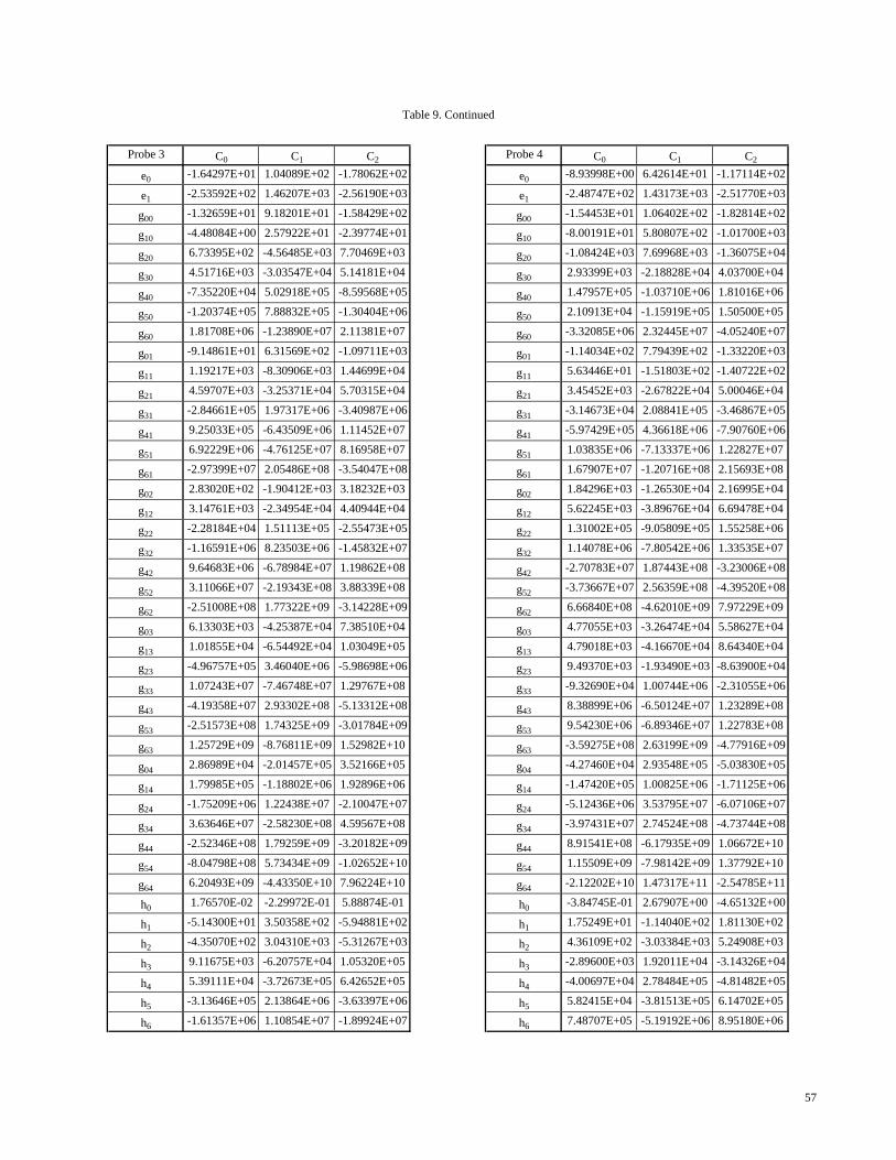
Probe 3 C0 C1 C2 Probe 4 C0 C1 C2

e0 -1.64297E+01 1.04089E+02 -1.78062E+02 e0 -8.93998E+00 6.42614E+01 -1.17114E+02

e1 -2.53592E+02 1.46207E+03 -2.56190E+03 e1 -2.48747E+02 1.43173E+03 -2.51770E+03

g00 -1.32659E+01 9.18201E+01 -1.58429E+02 g00 -1.54453E+01 1.06402E+02 -1.82814E+02

g10 -4.48084E+00 2.57922E+01 -2.39774E+01 g10 -8.00191E+01 5.80807E+02 -1.01700E+03

g20 6.73395E+02 -4.56485E+03 7.70469E+03 g20 -1.08424E+03 7.69968E+03 -1.36075E+04

g30 4.51716E+03 -3.03547E+04 5.14181E+04 g30 2.93399E+03 -2.18828E+04 4.03700E+04

g40 -7.35220E+04 5.02918E+05 -8.59568E+05 g40 1.47957E+05 -1.03710E+06 1.81016E+06

g50 -1.20374E+05 7.88832E+05 -1.30404E+06 g50 2.10913E+04 -1.15919E+05 1.50500E+05

g60 1.81708E+06 -1.23890E+07 2.11381E+07 g60 -3.32085E+06 2.32445E+07 -4.05240E+07

g01 -9.14861E+01 6.31569E+02 -1.09711E+03 g01 -1.14034E+02 7.79439E+02 -1.33220E+03

g11 1.19217E+03 -8.30906E+03 1.44699E+04 g11 5.63446E+01 -1.51803E+02 -1.40722E+02

g21 4.59707E+03 -3.25371E+04 5.70315E+04 g21 3.45452E+03 -2.67822E+04 5.00046E+04

g31 -2.84661E+05 1.97317E+06 -3.40987E+06 g31 -3.14673E+04 2.08841E+05 -3.46867E+05

g41 9.25033E+05 -6.43509E+06 1.11452E+07 g41 -5.97429E+05 4.36618E+06 -7.90760E+06

g51 6.92229E+06 -4.76125E+07 8.16958E+07 g51 1.03835E+06 -7.13337E+06 1.22827E+07

g61 -2.97399E+07 2.05486E+08 -3.54047E+08 g61 1.67907E+07 -1.20716E+08 2.15693E+08

g02 2.83020E+02 -1.90412E+03 3.18232E+03 g02 1.84296E+03 -1.26530E+04 2.16995E+04

g12 3.14761E+03 -2.34954E+04 4.40944E+04 g12 5.62245E+03 -3.89676E+04 6.69478E+04

g22 -2.28184E+04 1.51113E+05 -2.55473E+05 g22 1.31002E+05 -9.05809E+05 1.55258E+06

g32 -1.16591E+06 8.23503E+06 -1.45832E+07 g32 1.14078E+06 -7.80542E+06 1.33535E+07

g42 9.64683E+06 -6.78984E+07 1.19862E+08 g42 -2.70783E+07 1.87443E+08 -3.23006E+08

g52 3.11066E+07 -2.19343E+08 3.88339E+08 g52 -3.73667E+07 2.56359E+08 -4.39520E+08

g62 -2.51008E+08 1.77322E+09 -3.14228E+09 g62 6.66840E+08 -4.62010E+09 7.97229E+09

g03 6.13303E+03 -4.25387E+04 7.38510E+04 g03 4.77055E+03 -3.26474E+04 5.58627E+04

g13 1.01855E+04 -6.54492E+04 1.03049E+05 g13 4.79018E+03 -4.16670E+04 8.64340E+04

g23 -4.96757E+05 3.46040E+06 -5.98698E+06 g23 9.49370E+03 -1.93490E+03 -8.63900E+04

g33 1.07243E+07 -7.46748E+07 1.29767E+08 g33 -9.32690E+04 1.00744E+06 -2.31055E+06

g43 -4.19358E+07 2.93302E+08 -5.13312E+08 g43 8.38899E+06 -6.50124E+07 1.23289E+08

g53 -2.51573E+08 1.74325E+09 -3.01784E+09 g53 9.54230E+06 -6.89346E+07 1.22783E+08

g63 1.25729E+09 -8.76811E+09 1.52982E+10 g63 -3.59275E+08 2.63199E+09 -4.77916E+09

g04 2.86989E+04 -2.01457E+05 3.52166E+05 g04 -4.27460E+04 2.93548E+05 -5.03830E+05

g14 1.79985E+05 -1.18802E+06 1.92896E+06 g14 -1.47420E+05 1.00825E+06 -1.71125E+06

g24 -1.75209E+06 1.22438E+07 -2.10047E+07 g24 -5.12436E+06 3.53795E+07 -6.07106E+07

g34 3.63646E+07 -2.58230E+08 4.59567E+08 g34 -3.97431E+07 2.74524E+08 -4.73744E+08

g44 -2.52346E+08 1.79259E+09 -3.20182E+09 g44 8.91541E+08 -6.17935E+09 1.06672E+10

g54 -8.04798E+08 5.73434E+09 -1.02652E+10 g54 1.15509E+09 -7.98142E+09 1.37792E+10

g64 6.20493E+09 -4.43350E+10 7.96224E+10 g64 -2.12202E+10 1.47317E+11 -2.54785E+11

h0 1.76570E-02 -2.29972E-01 5.88874E-01 h0 -3.84745E-01 2.67907E+00 -4.65132E+00

h1 -5.14300E+01 3.50358E+02 -5.94881E+02 h1 1.75249E+01 -1.14040E+02 1.81130E+02

h2 -4.35070E+02 3.04310E+03 -5.31267E+03 h2 4.36109E+02 -3.03384E+03 5.24908E+03

h3 9.11675E+03 -6.20757E+04 1.05320E+05 h3 -2.89600E+03 1.92011E+04 -3.14326E+04

h4 5.39111E+04 -3.72673E+05 6.42652E+05 h4 -4.00697E+04 2.78484E+05 -4.81482E+05

h5 -3.13646E+05 2.13864E+06 -3.63397E+06 h5 5.82415E+04 -3.81513E+05 6.14702E+05

h6 -1.61357E+06 1.10854E+07 -1.89924E+07 h6 7.48707E+05 -5.19192E+06 8.95180E+06

Table 9. Continued

57

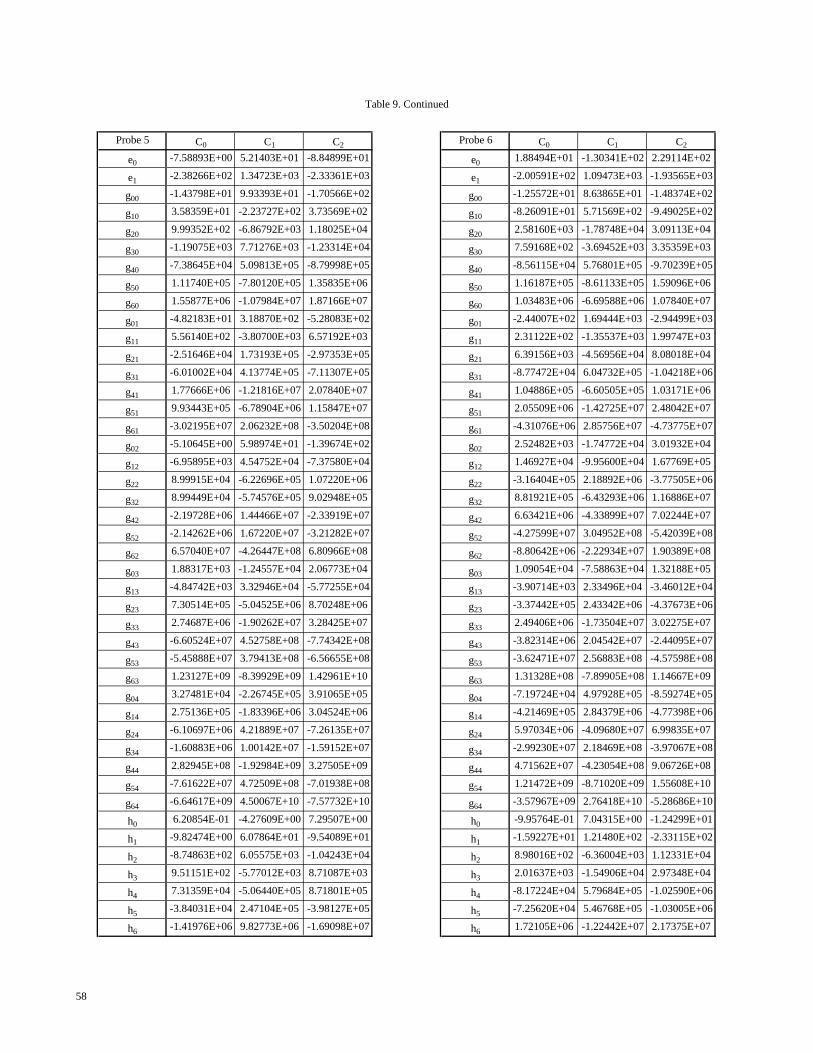
Probe 5 C0 C1 C2 Probe 6 C0 C1 C2

e0 -7.58893E+00 5.21403E+01 -8.84899E+01 e0 1.88494E+01 -1.30341E+02 2.29114E+02

e1 -2.38266E+02 1.34723E+03 -2.33361E+03 e1 -2.00591E+02 1.09473E+03 -1.93565E+03

g00 -1.43798E+01 9.93393E+01 -1.70566E+02 g00 -1.25572E+01 8.63865E+01 -1.48374E+02

g10 3.58359E+01 -2.23727E+02 3.73569E+02 g10 -8.26091E+01 5.71569E+02 -9.49025E+02

g20 9.99352E+02 -6.86792E+03 1.18025E+04 g20 2.58160E+03 -1.78748E+04 3.09113E+04

g30 -1.19075E+03 7.71276E+03 -1.23314E+04 g30 7.59168E+02 -3.69452E+03 3.35359E+03

g40 -7.38645E+04 5.09813E+05 -8.79998E+05 g40 -8.56115E+04 5.76801E+05 -9.70239E+05

g50 1.11740E+05 -7.80120E+05 1.35835E+06 g50 1.16187E+05 -8.61133E+05 1.59096E+06

g60 1.55877E+06 -1.07984E+07 1.87166E+07 g60 1.03483E+06 -6.69588E+06 1.07840E+07

g01 -4.82183E+01 3.18870E+02 -5.28083E+02 g01 -2.44007E+02 1.69444E+03 -2.94499E+03

g11 5.56140E+02 -3.80700E+03 6.57192E+03 g11 2.31122E+02 -1.35537E+03 1.99747E+03

g21 -2.51646E+04 1.73193E+05 -2.97353E+05 g21 6.39156E+03 -4.56956E+04 8.08018E+04

g31 -6.01002E+04 4.13774E+05 -7.11307E+05 g31 -8.77472E+04 6.04732E+05 -1.04218E+06

g41 1.77666E+06 -1.21816E+07 2.07840E+07 g41 1.04886E+05 -6.60505E+05 1.03171E+06

g51 9.93443E+05 -6.78904E+06 1.15847E+07 g51 2.05509E+06 -1.42725E+07 2.48042E+07

g61 -3.02195E+07 2.06232E+08 -3.50204E+08 g61 -4.31076E+06 2.85756E+07 -4.73775E+07

g02 -5.10645E+00 5.98974E+01 -1.39674E+02 g02 2.52482E+03 -1.74772E+04 3.01932E+04

g12 -6.95895E+03 4.54752E+04 -7.37580E+04 g12 1.46927E+04 -9.95600E+04 1.67769E+05

g22 8.99915E+04 -6.22696E+05 1.07220E+06 g22 -3.16404E+05 2.18892E+06 -3.77505E+06

g32 8.99449E+04 -5.74576E+05 9.02948E+05 g32 8.81921E+05 -6.43293E+06 1.16886E+07

g42 -2.19728E+06 1.44466E+07 -2.33919E+07 g42 6.63421E+06 -4.33899E+07 7.02244E+07

g52 -2.14262E+06 1.67220E+07 -3.21282E+07 g52 -4.27599E+07 3.04952E+08 -5.42039E+08

g62 6.57040E+07 -4.26447E+08 6.80966E+08 g62 -8.80642E+06 -2.22934E+07 1.90389E+08

g03 1.88317E+03 -1.24557E+04 2.06773E+04 g03 1.09054E+04 -7.58863E+04 1.32188E+05

g13 -4.84742E+03 3.32946E+04 -5.77255E+04 g13 -3.90714E+03 2.33496E+04 -3.46012E+04

g23 7.30514E+05 -5.04525E+06 8.70248E+06 g23 -3.37442E+05 2.43342E+06 -4.37673E+06

g33 2.74687E+06 -1.90262E+07 3.28425E+07 g33 2.49406E+06 -1.73504E+07 3.02275E+07

g43 -6.60524E+07 4.52758E+08 -7.74342E+08 g43 -3.82314E+06 2.04542E+07 -2.44095E+07

g53 -5.45888E+07 3.79413E+08 -6.56655E+08 g53 -3.62471E+07 2.56883E+08 -4.57598E+08

g63 1.23127E+09 -8.39929E+09 1.42961E+10 g63 1.31328E+08 -7.89905E+08 1.14667E+09

g04 3.27481E+04 -2.26745E+05 3.91065E+05 g04 -7.19724E+04 4.97928E+05 -8.59274E+05

g14 2.75136E+05 -1.83396E+06 3.04524E+06 g14 -4.21469E+05 2.84379E+06 -4.77398E+06

g24 -6.10697E+06 4.21889E+07 -7.26135E+07 g24 5.97034E+06 -4.09680E+07 6.99835E+07

g34 -1.60883E+06 1.00142E+07 -1.59152E+07 g34 -2.99230E+07 2.18469E+08 -3.97067E+08

g44 2.82945E+08 -1.92984E+09 3.27505E+09 g44 4.71562E+07 -4.23054E+08 9.06726E+08

g54 -7.61622E+07 4.72509E+08 -7.01938E+08 g54 1.21472E+09 -8.71020E+09 1.55608E+10

g64 -6.64617E+09 4.50067E+10 -7.57732E+10 g64 -3.57967E+09 2.76418E+10 -5.28686E+10

h0 6.20854E-01 -4.27609E+00 7.29507E+00 h0 -9.95764E-01 7.04315E+00 -1.24299E+01

h1 -9.82474E+00 6.07864E+01 -9.54089E+01 h1 -1.59227E+01 1.21480E+02 -2.33115E+02

h2 -8.74863E+02 6.05575E+03 -1.04243E+04 h2 8.98016E+02 -6.36004E+03 1.12331E+04

h3 9.51151E+02 -5.77012E+03 8.71087E+03 h3 2.01637E+03 -1.54906E+04 2.97348E+04

h4 7.31359E+04 -5.06440E+05 8.71801E+05 h4 -8.17224E+04 5.79684E+05 -1.02590E+06

h5 -3.84031E+04 2.47104E+05 -3.98127E+05 h5 -7.25620E+04 5.46768E+05 -1.03005E+06

h6 -1.41976E+06 9.82773E+06 -1.69098E+07 h6 1.72105E+06 -1.22442E+07 2.17375E+07

Table 9. Continued

58

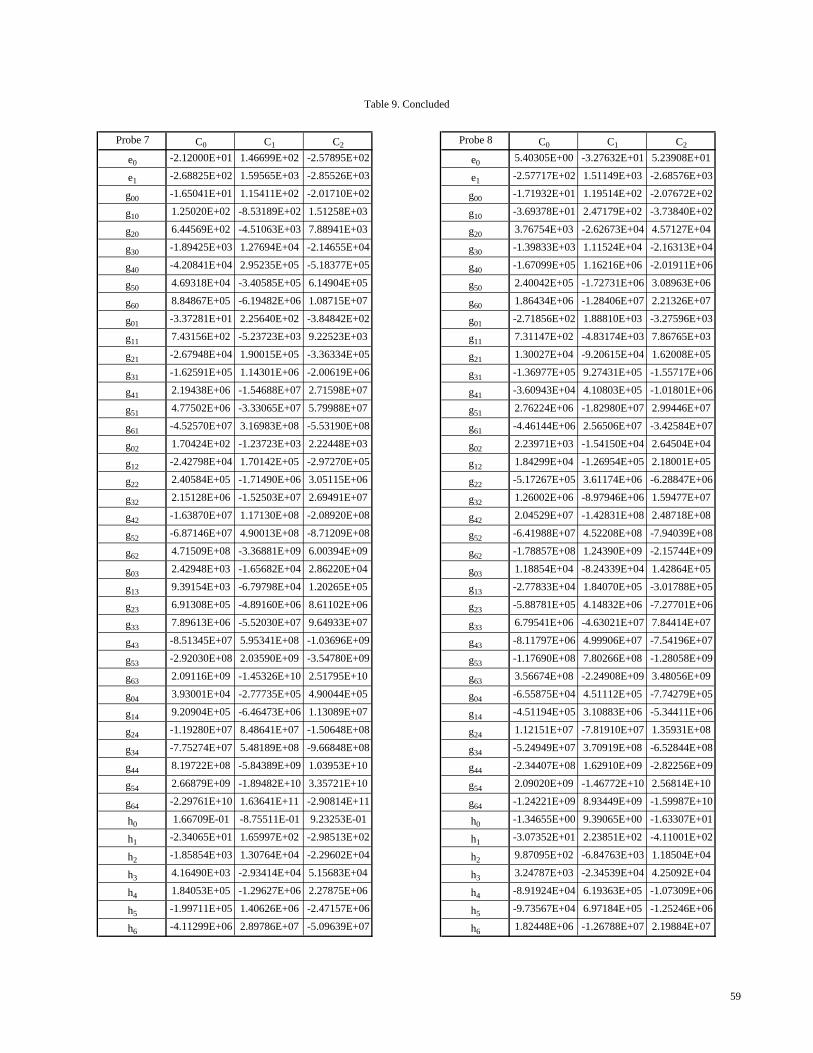
Probe 7 C0 C1 C2 Probe 8 C0 C1 C2

e0 -2.12000E+01 1.46699E+02 -2.57895E+02 e0 5.40305E+00 -3.27632E+01 5.23908E+01

e1 -2.68825E+02 1.59565E+03 -2.85526E+03 e1 -2.57717E+02 1.51149E+03 -2.68576E+03

g00 -1.65041E+01 1.15411E+02 -2.01710E+02 g00 -1.71932E+01 1.19514E+02 -2.07672E+02

g10 1.25020E+02 -8.53189E+02 1.51258E+03 g10 -3.69378E+01 2.47179E+02 -3.73840E+02

g20 6.44569E+02 -4.51063E+03 7.88941E+03 g20 3.76754E+03 -2.62673E+04 4.57127E+04

g30 -1.89425E+03 1.27694E+04 -2.14655E+04 g30 -1.39833E+03 1.11524E+04 -2.16313E+04

g40 -4.20841E+04 2.95235E+05 -5.18377E+05 g40 -1.67099E+05 1.16216E+06 -2.01911E+06

g50 4.69318E+04 -3.40585E+05 6.14904E+05 g50 2.40042E+05 -1.72731E+06 3.08963E+06

g60 8.84867E+05 -6.19482E+06 1.08715E+07 g60 1.86434E+06 -1.28406E+07 2.21326E+07

g01 -3.37281E+01 2.25640E+02 -3.84842E+02 g01 -2.71856E+02 1.88810E+03 -3.27596E+03

g11 7.43156E+02 -5.23723E+03 9.22523E+03 g11 7.31147E+02 -4.83174E+03 7.86765E+03

g21 -2.67948E+04 1.90015E+05 -3.36334E+05 g21 1.30027E+04 -9.20615E+04 1.62008E+05

g31 -1.62591E+05 1.14301E+06 -2.00619E+06 g31 -1.36977E+05 9.27431E+05 -1.55717E+06

g41 2.19438E+06 -1.54688E+07 2.71598E+07 g41 -3.60943E+04 4.10803E+05 -1.01801E+06

g51 4.77502E+06 -3.33065E+07 5.79988E+07 g51 2.76224E+06 -1.82980E+07 2.99446E+07

g61 -4.52570E+07 3.16983E+08 -5.53190E+08 g61 -4.46144E+06 2.56506E+07 -3.42584E+07

g02 1.70424E+02 -1.23723E+03 2.22448E+03 g02 2.23971E+03 -1.54150E+04 2.64504E+04

g12 -2.42798E+04 1.70142E+05 -2.97270E+05 g12 1.84299E+04 -1.26954E+05 2.18001E+05

g22 2.40584E+05 -1.71490E+06 3.05115E+06 g22 -5.17267E+05 3.61174E+06 -6.28847E+06

g32 2.15128E+06 -1.52503E+07 2.69491E+07 g32 1.26002E+06 -8.97946E+06 1.59477E+07

g42 -1.63870E+07 1.17130E+08 -2.08920E+08 g42 2.04529E+07 -1.42831E+08 2.48718E+08

g52 -6.87146E+07 4.90013E+08 -8.71209E+08 g52 -6.41988E+07 4.52208E+08 -7.94039E+08

g62 4.71509E+08 -3.36881E+09 6.00394E+09 g62 -1.78857E+08 1.24390E+09 -2.15744E+09

g03 2.42948E+03 -1.65682E+04 2.86220E+04 g03 1.18854E+04 -8.24339E+04 1.42864E+05

g13 9.39154E+03 -6.79798E+04 1.20265E+05 g13 -2.77833E+04 1.84070E+05 -3.01788E+05

g23 6.91308E+05 -4.89160E+06 8.61102E+06 g23 -5.88781E+05 4.14832E+06 -7.27701E+06

g33 7.89613E+06 -5.52030E+07 9.64933E+07 g33 6.79541E+06 -4.63021E+07 7.84414E+07

g43 -8.51345E+07 5.95341E+08 -1.03696E+09 g43 -8.11797E+06 4.99906E+07 -7.54196E+07

g53 -2.92030E+08 2.03590E+09 -3.54780E+09 g53 -1.17690E+08 7.80266E+08 -1.28058E+09

g63 2.09116E+09 -1.45326E+10 2.51795E+10 g63 3.56674E+08 -2.24908E+09 3.48056E+09

g04 3.93001E+04 -2.77735E+05 4.90044E+05 g04 -6.55875E+04 4.51112E+05 -7.74279E+05

g14 9.20904E+05 -6.46473E+06 1.13089E+07 g14 -4.51194E+05 3.10883E+06 -5.34411E+06

g24 -1.19280E+07 8.48641E+07 -1.50648E+08 g24 1.12151E+07 -7.81910E+07 1.35931E+08

g34 -7.75274E+07 5.48189E+08 -9.66848E+08 g34 -5.24949E+07 3.70919E+08 -6.52844E+08

g44 8.19722E+08 -5.84389E+09 1.03953E+10 g44 -2.34407E+08 1.62910E+09 -2.82256E+09

g54 2.66879E+09 -1.89482E+10 3.35721E+10 g54 2.09020E+09 -1.46772E+10 2.56814E+10

g64 -2.29761E+10 1.63641E+11 -2.90814E+11 g64 -1.24221E+09 8.93449E+09 -1.59987E+10

h0 1.66709E-01 -8.75511E-01 9.23253E-01 h0 -1.34655E+00 9.39065E+00 -1.63307E+01

h1 -2.34065E+01 1.65997E+02 -2.98513E+02 h1 -3.07352E+01 2.23851E+02 -4.11001E+02

h2 -1.85854E+03 1.30764E+04 -2.29602E+04 h2 9.87095E+02 -6.84763E+03 1.18504E+04

h3 4.16490E+03 -2.93414E+04 5.15683E+04 h3 3.24787E+03 -2.34539E+04 4.25092E+04

h4 1.84053E+05 -1.29627E+06 2.27875E+06 h4 -8.91924E+04 6.19363E+05 -1.07309E+06

h5 -1.99711E+05 1.40626E+06 -2.47157E+06 h5 -9.73567E+04 6.97184E+05 -1.25246E+06

h6 -4.11299E+06 2.89786E+07 -5.09639E+07 h6 1.82448E+06 -1.26788E+07 2.19884E+07

Table 9. Concluded

59

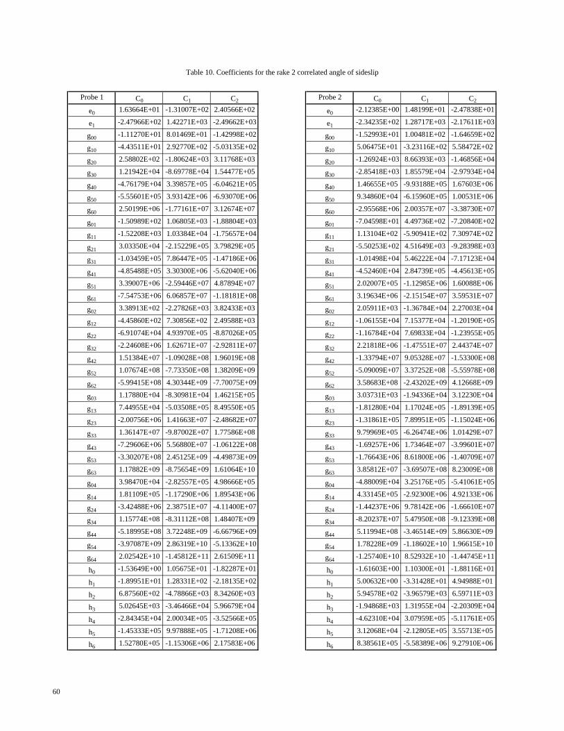
Probe 1 C0 C1 C2 Probe 2 C0 C1 C2

e0 1.63664E+01 -1.31007E+02 2.40566E+02 e0 -2.12385E+00 1.48199E+01 -2.47838E+01

e1 -2.47966E+02 1.42271E+03 -2.49662E+03 e1 -2.34235E+02 1.28717E+03 -2.17611E+03

g00 -1.11270E+01 8.01469E+01 -1.42998E+02 g00 -1.52993E+01 1.00481E+02 -1.64659E+02

g10 -4.43511E+01 2.92770E+02 -5.03135E+02 g10 5.06475E+01 -3.23116E+02 5.58472E+02

g20 2.58802E+02 -1.80624E+03 3.11768E+03 g20 -1.26924E+03 8.66393E+03 -1.46856E+04

g30 1.21942E+04 -8.69778E+04 1.54477E+05 g30 -2.85418E+03 1.85579E+04 -2.97934E+04

g40 -4.76179E+04 3.39857E+05 -6.04621E+05 g40 1.46655E+05 -9.93188E+05 1.67603E+06

g50 -5.55601E+05 3.93142E+06 -6.93070E+06 g50 9.34860E+04 -6.15960E+05 1.00531E+06

g60 2.50199E+06 -1.77161E+07 3.12674E+07 g60 -2.95568E+06 2.00357E+07 -3.38730E+07

g01 -1.50989E+02 1.06805E+03 -1.88804E+03 g01 -7.04598E+01 4.49736E+02 -7.20840E+02

g11 -1.52208E+03 1.03384E+04 -1.75657E+04 g11 1.13104E+02 -5.90941E+02 7.30974E+02

g21 3.03350E+04 -2.15229E+05 3.79829E+05 g21 -5.50253E+02 4.51649E+03 -9.28398E+03

g31 -1.03459E+05 7.86447E+05 -1.47186E+06 g31 -1.01498E+04 5.46222E+04 -7.17123E+04

g41 -4.85488E+05 3.30300E+06 -5.62040E+06 g41 -4.52460E+04 2.84739E+05 -4.45613E+05

g51 3.39007E+06 -2.59446E+07 4.87894E+07 g51 2.02007E+05 -1.12985E+06 1.60088E+06

g61 -7.54753E+06 6.06857E+07 -1.18181E+08 g61 3.19634E+06 -2.15154E+07 3.59531E+07

g02 3.38913E+02 -2.27826E+03 3.82433E+03 g02 2.05911E+03 -1.36784E+04 2.27003E+04

g12 -4.45860E+02 7.30856E+02 2.49588E+03 g12 -1.06155E+04 7.15377E+04 -1.20190E+05

g22 -6.91074E+04 4.93970E+05 -8.87026E+05 g22 -1.16784E+04 7.69833E+04 -1.23955E+05

g32 -2.24608E+06 1.62671E+07 -2.92811E+07 g32 2.21818E+06 -1.47551E+07 2.44374E+07

g42 1.51384E+07 -1.09028E+08 1.96019E+08 g42 -1.33794E+07 9.05328E+07 -1.53300E+08

g52 1.07674E+08 -7.73350E+08 1.38209E+09 g52 -5.09009E+07 3.37252E+08 -5.55978E+08

g62 -5.99415E+08 4.30344E+09 -7.70075E+09 g62 3.58683E+08 -2.43202E+09 4.12668E+09

g03 1.17880E+04 -8.30981E+04 1.46215E+05 g03 3.03731E+03 -1.94336E+04 3.12230E+04

g13 7.44955E+04 -5.03508E+05 8.49550E+05 g13 -1.81280E+04 1.17024E+05 -1.89139E+05

g23 -2.00756E+06 1.41663E+07 -2.48682E+07 g23 -1.31861E+05 7.89951E+05 -1.15024E+06

g33 1.36147E+07 -9.87002E+07 1.77586E+08 g33 9.79969E+05 -6.26474E+06 1.01429E+07

g43 -7.29606E+06 5.56880E+07 -1.06122E+08 g43 -1.69257E+06 1.73464E+07 -3.99601E+07

g53 -3.30207E+08 2.45125E+09 -4.49873E+09 g53 -1.76643E+06 8.61800E+06 -1.40709E+07

g63 1.17882E+09 -8.75654E+09 1.61064E+10 g63 3.85812E+07 -3.69507E+08 8.23009E+08

g04 3.98470E+04 -2.82557E+05 4.98666E+05 g04 -4.88009E+04 3.25176E+05 -5.41061E+05

g14 1.81109E+05 -1.17290E+06 1.89543E+06 g14 4.33145E+05 -2.92300E+06 4.92133E+06

g24 -3.42488E+06 2.38751E+07 -4.11400E+07 g24 -1.44237E+06 9.78142E+06 -1.66610E+07

g34 1.15774E+08 -8.31112E+08 1.48407E+09 g34 -8.20237E+07 5.47950E+08 -9.12339E+08

g44 -5.18995E+08 3.72248E+09 -6.66796E+09 g44 5.11994E+08 -3.46514E+09 5.86630E+09

g54 -3.97087E+09 2.86319E+10 -5.13362E+10 g54 1.78228E+09 -1.18602E+10 1.96615E+10

g64 2.02542E+10 -1.45812E+11 2.61509E+11 g64 -1.25740E+10 8.52932E+10 -1.44745E+11

h0 -1.53649E+00 1.05675E+01 -1.82287E+01 h0 -1.61603E+00 1.10300E+01 -1.88116E+01

h1 -1.89951E+01 1.28331E+02 -2.18135E+02 h1 5.00632E+00 -3.31428E+01 4.94988E+01

h2 6.87560E+02 -4.78866E+03 8.34260E+03 h2 5.94578E+02 -3.96579E+03 6.59711E+03

h3 5.02645E+03 -3.46466E+04 5.96679E+04 h3 -1.94868E+03 1.31955E+04 -2.20309E+04

h4 -2.84345E+04 2.00034E+05 -3.52566E+05 h4 -4.62310E+04 3.07959E+05 -5.11761E+05

h5 -1.45333E+05 9.97888E+05 -1.71208E+06 h5 3.12068E+04 -2.12805E+05 3.55713E+05

h6 1.52780E+05 -1.15306E+06 2.17583E+06 h6 8.38561E+05 -5.58389E+06 9.27910E+06

Table 10. Coefficients for the rake 2 correlated angle of sideslip

60

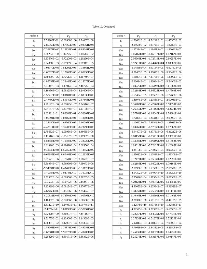
Probe 3 C0 C1 C2 Probe 4 C0 C1 C2

e0 7.50908E-01 -3.39968E+00 8.74067E+00 e0 -1.50631E+01 8.74240E+01 -1.45353E+02

e1 -2.85366E+02 1.67965E+03 -2.93561E+03 e1 -2.04670E+02 1.09721E+03 -1.87859E+03

g00 -7.37971E+00 5.12938E+01 -8.85241E+01 g00 -1.67334E+01 1.11498E+02 -1.82093E+02

g10 8.28284E+00 -6.44275E+01 1.11613E+02 g10 1.06160E+02 -6.66512E+02 1.12162E+03

g20 9.33676E+02 -6.72200E+03 1.20260E+04 g20 2.56669E+03 -1.72719E+04 2.90257E+04

g30 8.04358E+03 -5.71969E+04 1.01312E+05 g30 8.92419E+03 -6.24780E+04 1.08607E+05

g40 -1.04970E+05 7.54292E+05 -1.34861E+06 g40 -6.04859E+04 4.00154E+05 -6.62767E+05

g50 -1.66025E+05 1.17203E+06 -2.06290E+06 g50 -5.09403E+05 3.50093E+06 -5.98472E+06

g60 2.48009E+06 -1.77613E+07 3.16740E+07 g60 -1.11864E+06 7.83705E+06 -1.35956E+07

g01 -1.85757E+02 1.26449E+03 -2.15075E+03 g01 -2.62614E+01 1.83064E+02 -3.24900E+02

g11 2.03847E+03 -1.41914E+04 2.46775E+04 g11 1.03725E+03 -6.36492E+03 9.61288E+03

g21 4.18036E+03 -2.68325E+04 4.24606E+04 g21 1.32183E+04 -8.86328E+04 1.47809E+05

g31 -1.57415E+05 1.09101E+06 -1.88336E+06 g31 -1.69494E+05 1.08565E+06 -1.72600E+06

g41 -2.47490E+05 1.59349E+06 -2.57668E+06 g41 -1.81978E+06 1.20850E+07 -2.00089E+07

g51 1.99192E+06 -1.37025E+07 2.34516E+07 g51 5.36782E+06 -3.47203E+07 5.58059E+07

g61 8.04187E+06 -5.43748E+07 9.23178E+07 g61 4.26055E+07 -2.81168E+08 4.62234E+08

g02 1.02881E+01 5.86389E+01 -3.52207E+02 g02 1.57761E+03 -1.05040E+04 1.74801E+04

g12 -1.05591E+04 7.08167E+04 -1.18603E+05 g12 -1.77895E+04 1.20448E+05 -2.03907E+05

g22 -2.38150E+05 1.69560E+06 -3.00298E+06 g22 -1.10622E+05 7.51540E+05 -1.28013E+06

g32 -4.43514E+05 3.35208E+06 -6.23499E+06 g32 1.03765E+06 -6.97335E+06 1.17667E+07

g42 2.75662E+07 -1.95958E+08 3.46665E+08 g42 -6.94407E+05 4.37731E+06 -6.31212E+06

g52 8.13516E+06 -6.25137E+07 1.17987E+08 g52 8.88152E+06 -6.15715E+07 1.03525E+08

g62 -5.84586E+08 4.16386E+09 -7.38029E+09 g62 1.33980E+08 -9.06109E+08 1.51352E+09

g03 6.61996E+03 -4.48690E+04 7.60556E+04 g03 1.05815E+03 -7.72425E+03 1.42805E+04

g13 -9.41046E+04 6.55655E+05 -1.13859E+06 g13 -9.24158E+04 5.79002E+05 -8.96257E+05

g23 -9.69985E+05 6.60408E+06 -1.12135E+07 g23 -1.65012E+06 1.10830E+07 -1.85309E+07

g33 7.35671E+06 -5.09548E+07 8.78627E+07 g33 1.12470E+07 -7.15830E+07 1.12891E+08

g43 6.80984E+07 -4.66950E+08 7.99073E+08 g43 1.62189E+08 -1.08029E+09 1.79180E+09

g53 -9.34091E+07 6.43400E+08 -1.10120E+09 g53 -2.58950E+08 1.63530E+09 -2.55570E+09

g63 -1.49087E+09 1.02744E+10 -1.76734E+10 g63 -2.94302E+09 1.94004E+10 -3.18295E+10

g04 2.52562E+04 -1.80356E+05 3.20233E+05 g04 -2.85096E+04 1.87354E+05 -3.07508E+05

g14 5.57573E+05 -3.80772E+06 6.49247E+06 g14 4.29124E+04 -4.50049E+05 1.04750E+06

g24 7.23939E+06 -5.08154E+07 8.87677E+07 g24 -4.80055E+06 3.20564E+07 -5.31529E+07

g34 -4.62460E+05 -5.15166E+06 2.25424E+07 g34 1.38259E+07 -7.75629E+07 1.01119E+08

g44 -8.20831E+08 5.78304E+09 -1.01398E+10 g44 6.10468E+08 -4.05999E+09 6.71462E+09

g54 1.16092E+08 -5.92066E+08 6.66500E+08 g54 -8.76320E+08 5.50103E+09 -8.47199E+09

g64 1.61221E+10 -1.14063E+11 2.00748E+11 g64 -1.22579E+10 8.09756E+10 -1.32886E+11

h0 -2.48774E-01 1.88198E+00 -3.52794E+00 h0 -4.80525E+00 3.28337E+01 -5.66965E+01

h1 3.52020E+00 -3.46097E+01 7.49116E+01 h1 1.22257E+01 -8.84939E+01 1.47631E+02

h2 1.51755E+02 -1.13900E+03 2.14369E+03 h2 2.27932E+02 -1.51378E+03 2.52120E+03

h3 4.86351E+02 -2.42007E+03 2.85363E+03 h3 -5.97843E+03 4.11857E+04 -7.08001E+04

h4 -1.83168E+04 1.33833E+05 -2.45753E+05 h4 -3.76619E+04 2.54281E+05 -4.29506E+05

h5 -1.68984E+04 9.91873E+04 -1.49400E+05 h5 1.45435E+05 -1.00829E+06 1.74236E+06

h6 5.29429E+05 -3.80171E+06 6.86362E+06 h6 8.25279E+05 -5.63157E+06 9.60147E+06

Table 10. Continued

61

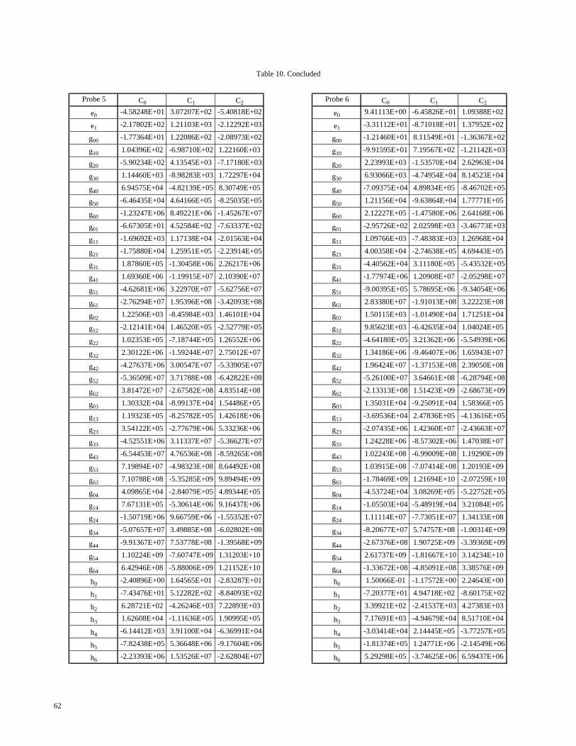
Probe 5 C0 C1 C2 Probe 6 C0 C1 C2

e0 -4.58248E+01 3.07207E+02 -5.40818E+02 e0 9.41113E+00 -6.45826E+01 1.09388E+02

e1 -2.17802E+02 1.21103E+03 -2.12292E+03 e1 -3.31112E+01 -8.71018E+01 1.37952E+02

g00 -1.77364E+01 1.22086E+02 -2.08973E+02 g00 -1.21460E+01 8.11549E+01 -1.36367E+02

g10 1.04396E+02 -6.98710E+02 1.22160E+03 g10 -9.91595E+01 7.19567E+02 -1.21142E+03

g20 -5.90234E+02 4.13545E+03 -7.17180E+03 g20 2.23993E+03 -1.53570E+04 2.62963E+04

g30 1.14460E+03 -8.98283E+03 1.72297E+04 g30 6.93066E+03 -4.74954E+04 8.14523E+04

g40 6.94575E+04 -4.82139E+05 8.30749E+05 g40 -7.09375E+04 4.89834E+05 -8.46702E+05

g50 -6.46435E+04 4.64166E+05 -8.25035E+05 g50 1.21156E+04 -9.63864E+04 1.77771E+05

g60 -1.23247E+06 8.49221E+06 -1.45267E+07 g60 2.12227E+05 -1.47580E+06 2.64168E+06

g01 -6.67305E+01 4.52584E+02 -7.63337E+02 g01 -2.95726E+02 2.02598E+03 -3.46773E+03

g11 -1.69692E+03 1.17138E+04 -2.01563E+04 g11 1.09766E+03 -7.48383E+03 1.26968E+04

g21 -1.75880E+04 1.25951E+05 -2.23914E+05 g21 4.00358E+04 -2.74638E+05 4.69443E+05

g31 1.87860E+05 -1.30458E+06 2.26217E+06 g31 -4.40562E+04 3.11180E+05 -5.43532E+05

g41 1.69360E+06 -1.19915E+07 2.10390E+07 g41 -1.77974E+06 1.20908E+07 -2.05298E+07

g51 -4.62681E+06 3.22970E+07 -5.62756E+07 g51 -9.00395E+05 5.78695E+06 -9.34054E+06

g61 -2.76294E+07 1.95396E+08 -3.42093E+08 g61 2.83380E+07 -1.91013E+08 3.22223E+08

g02 1.22506E+03 -8.45984E+03 1.46101E+04 g02 1.50115E+03 -1.01490E+04 1.71251E+04

g12 -2.12141E+04 1.46520E+05 -2.52779E+05 g12 9.85623E+03 -6.42635E+04 1.04024E+05

g22 1.02353E+05 -7.18744E+05 1.26552E+06 g22 -4.64180E+05 3.21362E+06 -5.54939E+06

g32 2.30122E+06 -1.59244E+07 2.75012E+07 g32 1.34186E+06 -9.46407E+06 1.65943E+07

g42 -4.27637E+06 3.00547E+07 -5.33905E+07 g42 1.96424E+07 -1.37153E+08 2.39050E+08

g52 -5.36509E+07 3.71788E+08 -6.42822E+08 g52 -5.26100E+07 3.64661E+08 -6.28794E+08

g62 3.81472E+07 -2.67582E+08 4.83514E+08 g62 -2.13313E+08 1.51423E+09 -2.68673E+09

g03 1.30332E+04 -8.99137E+04 1.54486E+05 g03 1.35031E+04 -9.25091E+04 1.58366E+05

g13 1.19323E+05 -8.25782E+05 1.42618E+06 g13 -3.69536E+04 2.47836E+05 -4.13616E+05

g23 3.54122E+05 -2.77679E+06 5.33236E+06 g23 -2.07435E+06 1.42360E+07 -2.43663E+07

g33 -4.52551E+06 3.11337E+07 -5.36627E+07 g33 1.24228E+06 -8.57302E+06 1.47038E+07

g43 -6.54453E+07 4.76536E+08 -8.59265E+08 g43 1.02243E+08 -6.99009E+08 1.19290E+09

g53 7.19894E+07 -4.98323E+08 8.64492E+08 g53 1.03915E+08 -7.07414E+08 1.20193E+09

g63 7.10788E+08 -5.35285E+09 9.89494E+09 g63 -1.78469E+09 1.21694E+10 -2.07259E+10

g04 4.09865E+04 -2.84079E+05 4.89344E+05 g04 -4.53724E+04 3.08269E+05 -5.22752E+05

g14 7.67131E+05 -5.30614E+06 9.16437E+06 g14 -1.05503E+04 -5.48919E+04 3.21084E+05

g24 -1.50719E+06 9.66759E+06 -1.55352E+07 g24 1.11114E+07 -7.73051E+07 1.34133E+08

g34 -5.07657E+07 3.49885E+08 -6.02802E+08 g34 -8.20677E+07 5.74757E+08 -1.00314E+09

g44 -9.91367E+07 7.53778E+08 -1.39568E+09 g44 -2.67376E+08 1.90725E+09 -3.39369E+09

g54 1.10224E+09 -7.60747E+09 1.31203E+10 g54 2.61737E+09 -1.81667E+10 3.14234E+10

g64 6.42946E+08 -5.88006E+09 1.21152E+10 g64 -1.33672E+08 -4.85091E+08 3.38576E+09

h0 -2.40896E+00 1.64565E+01 -2.83287E+01 h0 1.50066E-01 -1.17572E+00 2.24643E+00

h1 -7.43476E+01 5.12282E+02 -8.84093E+02 h1 -7.20377E+01 4.94718E+02 -8.60175E+02

h2 6.28721E+02 -4.26246E+03 7.22893E+03 h2 3.39921E+02 -2.41537E+03 4.27383E+03

h3 1.62608E+04 -1.11636E+05 1.90995E+05 h3 7.17691E+03 -4.94679E+04 8.51710E+04

h4 -6.14412E+03 3.91100E+04 -6.36991E+04 h4 -3.03414E+04 2.14445E+05 -3.77257E+05

h5 -7.82438E+05 5.36648E+06 -9.17604E+06 h5 -1.81374E+05 1.24771E+06 -2.14549E+06

h6 -2.23393E+06 1.53526E+07 -2.62804E+07 h6 5.29298E+05 -3.74625E+06 6.59437E+06

Table 10. Concluded

62

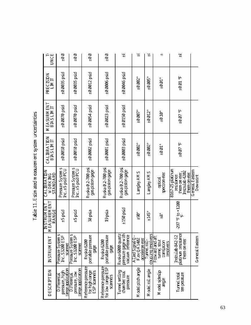
63

64

Figure 1. Mach number error due to total pressure recovery.

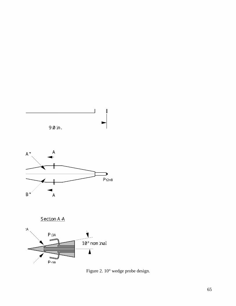
65

Figure 2. 10° wedge probe design.

66

Figure 3. 4 X 4 cone-probe rake assembly.

67

Figure 4. 2 X 4 cone-probe rake assembly.

68

Figure 5. 2 X 3 cone-probe rake assembly.

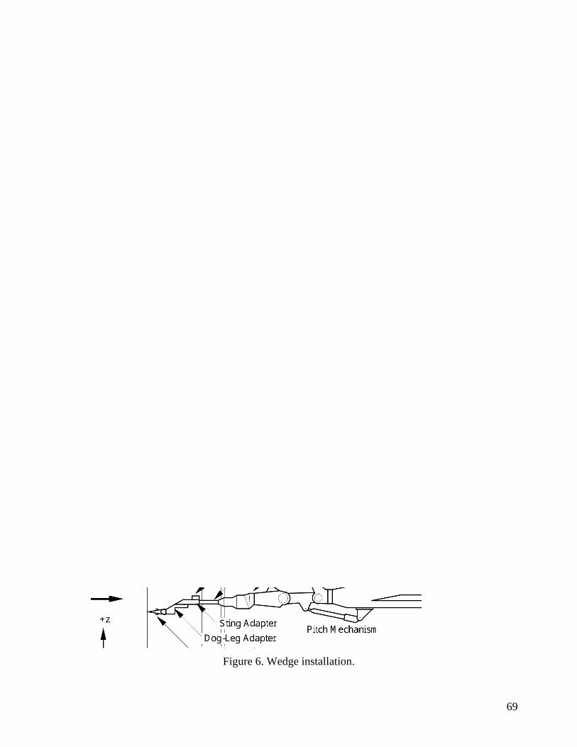
69

Figure 6. Wedge installation.

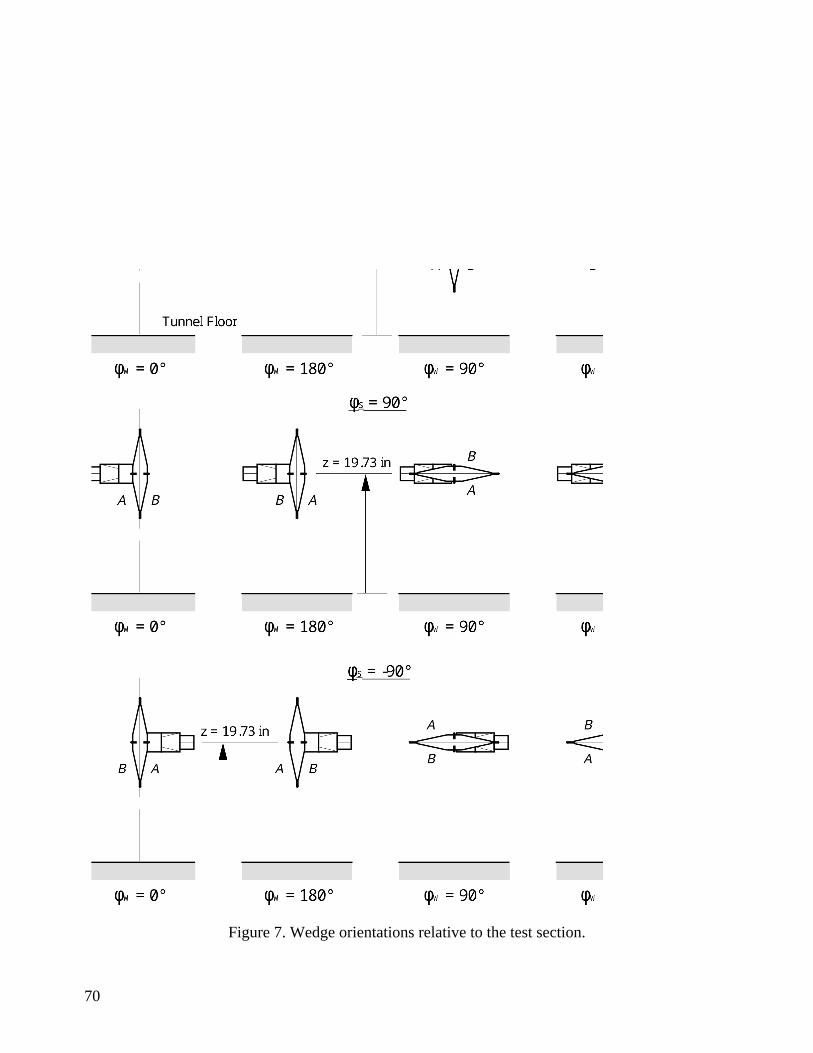
70

Figure 7. Wedge orientations relative to the test section.

71

Figure 8. Cone-probe rake installation.

72

Figure 9. Wedge positioning for cone-probe calibration.

73

Figure 10. Measured sting adapter to model pitch angle relationship.

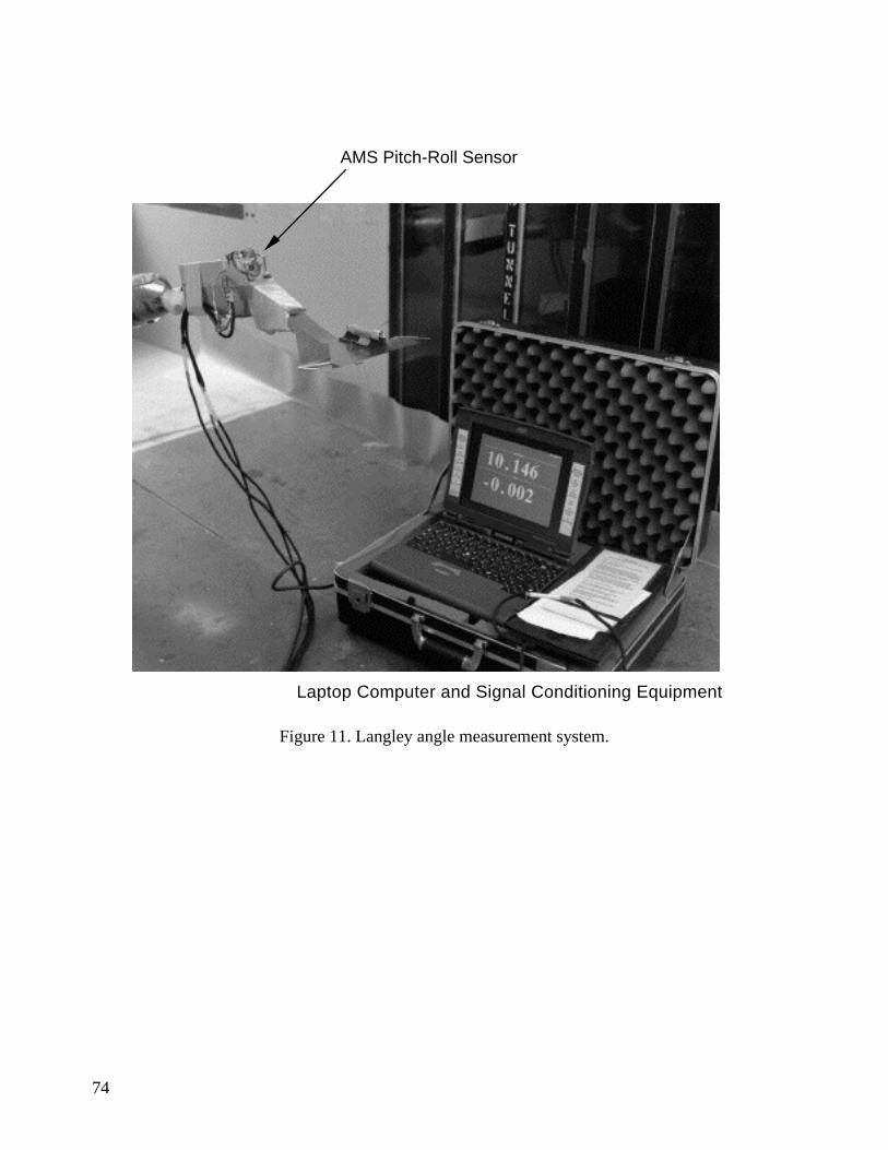
74

AMS Pitch-Roll Sensor

Laptop Computer and Signal Conditioning Equipment

Figure 11. Langley angle measurement system.

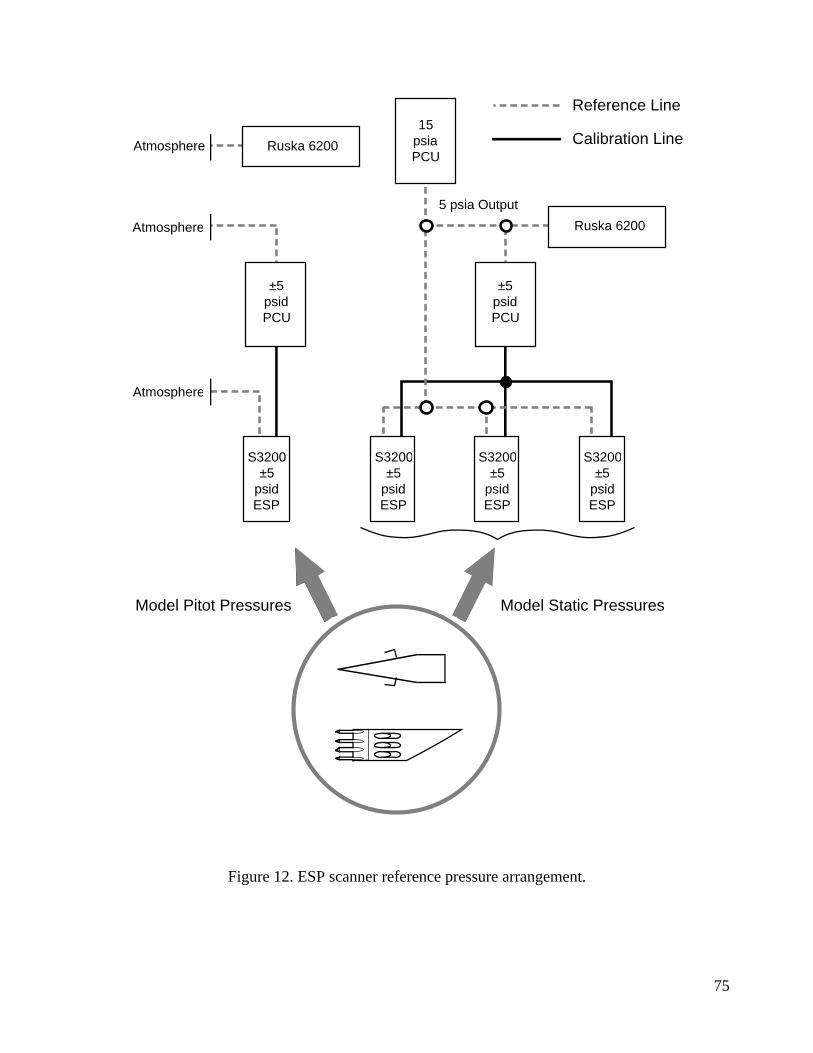
75

S3200±5

psid ESP

±5 psid PCU

Atmosphere

15 psia PCU

±5 psid PCU

S3200±5

psid ESP

S3200±5

psid ESP

S3200±5

psid ESP

Atmosphere Ruska 6200

Ruska 6200Atmosphere

Reference Line

Calibration Line

Model Static PressuresModel Pitot Pressures

5 psia Output

Figure 12. ESP scanner reference pressure arrangement.

76

Figure 13. General wedge flow relationship.

77

Figure 14. Complementary wedge pressure and geometric variables.

Figure 15. Boundary layer displacement effect on oblique shock.

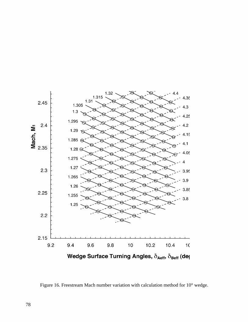
78

Figure 16. Freestream Mach number variation with calculation method for 10° wedge.

79

Figure 17. Freestream normal shock recovery distribution.

80

Figure 18. Wedge angle of attack sensitivity to static pressure ratio.

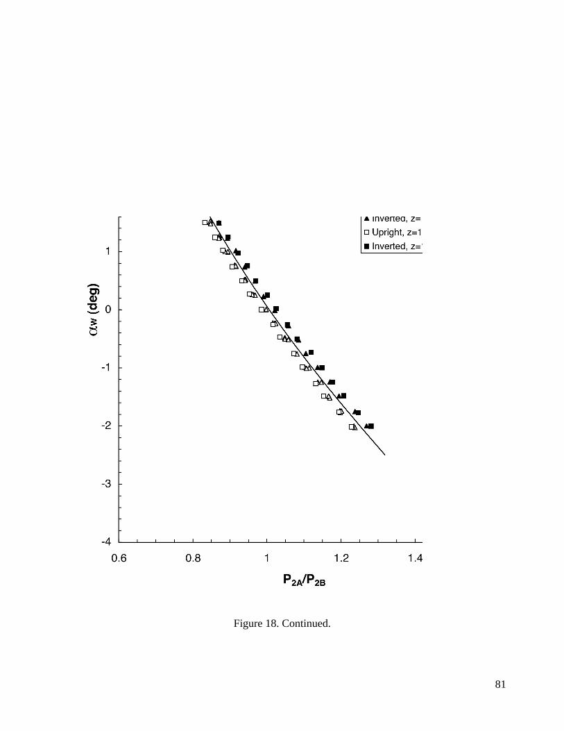
81

Figure 18. Continued.

82

Figure 18. Concluded.

Figure 19. Tunnel upflow and crossflow derivation.

-3

-2

-1

0

1

2

3

-2 -1 0 1 2 3 4

αWcorr (deg)

ε (d

eg)

µ = -ε0 = 1.311°

-3

-2

-1

0

1

2

3

-2 -1 0 1 2 3 4

αWcorr (deg)

ε (d

eg)

µ = -ε0 = 1.428°

-3

-2

-1

0

1

2

3

-3 -2 -1 0 1 2 3

αWcorr (deg)

ψ (

deg

)

ξ = ψ0 = -0.077°

-3

-2

-1

0

1

2

3

-3 -2 -1 0 1 2 3

αWcorr (deg)

ψ (

deg

)

ξ = ψ0 = -0.045°

z = 16.24 in

z = 19.73 in

Upflow Crossflow

UPWT Test Section 1, Mset = 2.15

83

Figure 19. Continued.

-3

-2

-1

0

1

2

3

-3 -2 -1 0 1 2 3

αWcorr (deg)

ε (d

eg)

µ = -ε0 = 0.121°

-3

-2

-1

0

1

2

3

-3 -2 -1 0 1 2 3

αWcorr (deg)

ε (d

eg)

µ = -ε0 = 0.193°

-3

-2

-1

0

1

2

3

-3 -2 -1 0 1 2 3

αWcorr (deg)

ψ (

deg

)

ξ = ψ0 = 0.078°

-3

-2

-1

0

1

2

3

-3 -2 -1 0 1 2 3

αWcorr (deg)

ψ (

deg

)

ξ = ψ0 = 0.134°

z = 16.24 in

z = 19.73 in

Upflow Crossflow

UPWT Test Section 2, Mset = 2.29

84

Figure 19. Concluded.

-3

-2

-1

0

1

2

3

-3 -2 -1 0 1 2 3

αWcorr (deg)

ε (d

eg)

µ = -ε0 = -0.141°

-3

-2

-1

0

1

2

3

-3 -2 -1 0 1 2 3

αWcorr (deg)

ε (d

eg)

µ = -ε0 = 0.030°

-3

-2

-1

0

1

2

3

-3 -2 -1 0 1 2 3

αWcorr (deg)

ψ (

deg

)

ξ = ψ0 = 0.093°

-3

-2

-1

0

1

2

3

-3 -2 -1 0 1 2 3

αWcorr (deg)

ψ (

deg

)

ξ = ψ0 = 0.139°

z = 16.24 in

z = 19.73 in

Upflow Crossflow

UPWT Test Section 2, Mset = 2.40

85

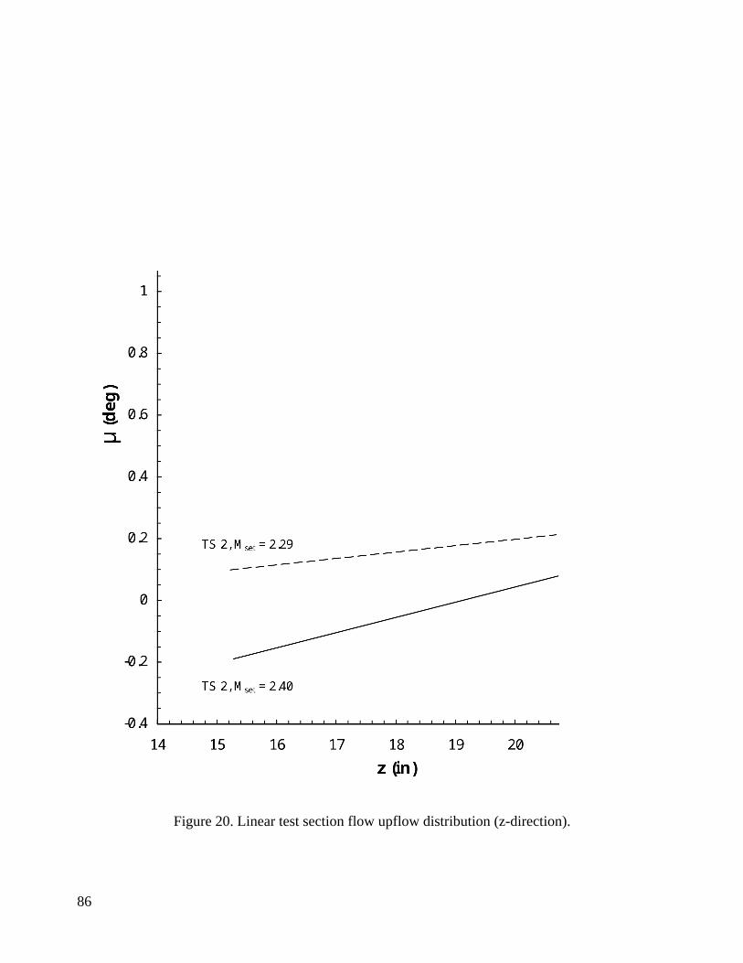
86

Figure 20. Linear test section flow upflow distribution (z-direction).

87

Figure 21. Linear test section flow crossflow distribution (z-direction).

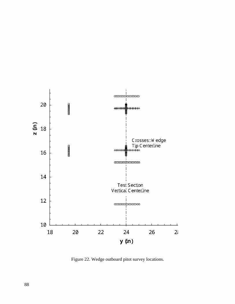
88

Figure 22. Wedge outboard pitot survey locations.

Figure 23. Linear test section Mach number distribution (z-cirection) for variouscalculation methods.

2.36

2.37

2.38

2.39

2.4

2.41

2.42

2.43

15 16 17 18 19 20

z (in)

M1

Mset = 2.40

2.25

2.26

2.27

2.28

2.29

2.3

2.31

2.32

15 16 17 18 19 20

z (in)

M1

Method I

Method II

Method III

Perfect Recovery

Mset = 2.29

2.11

2.12

2.13

2.14

2.15

2.16

2.17

2.18

15 16 17 18 19 20

z (in)

M1

Mset = 2.15

UPWT TS 2UPWT TS 1

UPWT TS 2

89

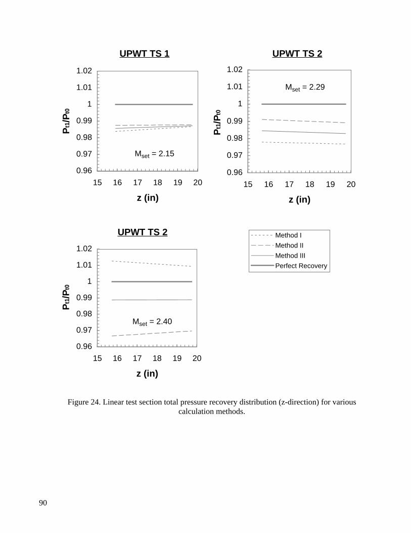
Figure 24. Linear test section total pressure recovery distribution (z-direction) for variouscalculation methods.

0.96

0.97

0.98

0.99

1

1.01

1.02

15 16 17 18 19 20

z (in)

Pt1

/Pt0

Mset = 2.40

0.96

0.97

0.98

0.99

1

1.01

1.02

15 16 17 18 19 20

z (in)

Pt1

/Pt0

Method I

Method II

Method III

Perfect Recovery

Mset = 2.29

0.96

0.97

0.98

0.99

1

1.01

1.02

15 16 17 18 19 20

z (in)

Pt1

/Pt0

Mset = 2.15

UPWT TS 2UPWT TS 1

UPWT TS 2

90

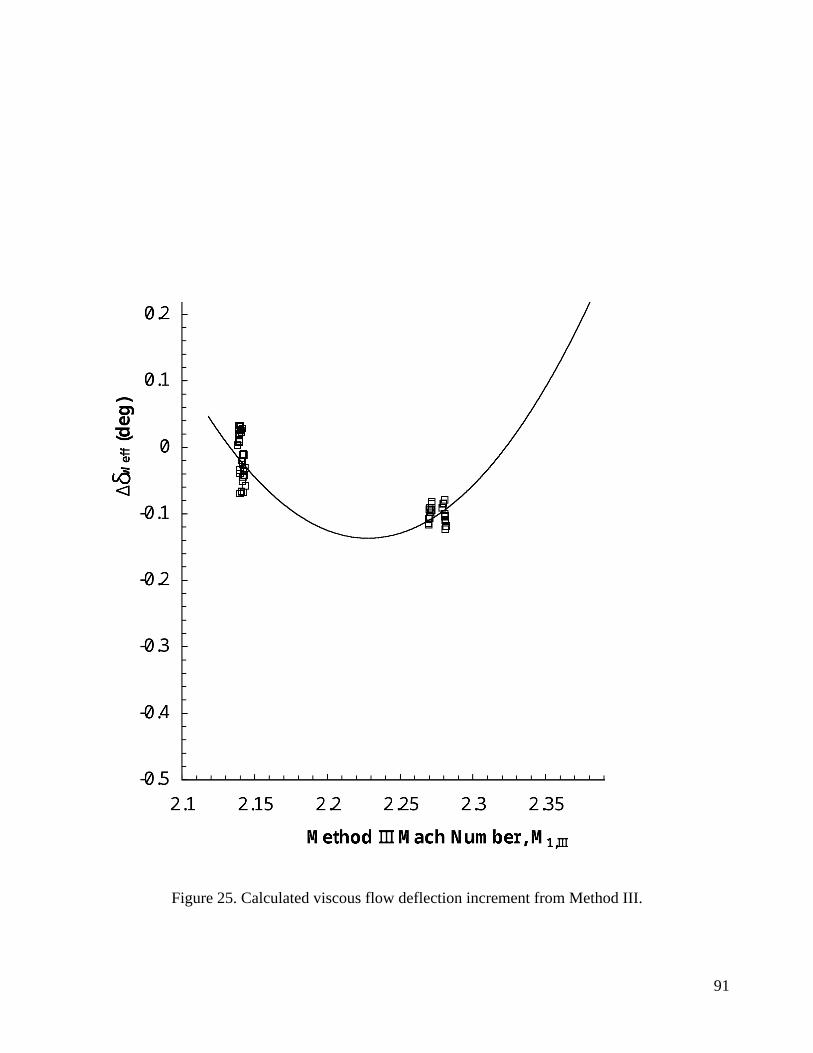
91

Figure 25. Calculated viscous flow deflection increment from Method III.

Figure 26. Comparison of Mach number sensitivity to wedge inclination.

8°

10°

12°

-40

-30

-20

-10

0

2 2.1 2.2 2.3 2.4 2.5

M1

(∆M

1/M

1)/(

∆P2/

P2)

Method II Mach Sensitivity

δ (deg)

8°

10°

12°

1

2

3

4

5

2 2.1 2.2 2.3 2.4 2.5

(∆M

1/M

1)/(

∆Pt3/P

t3)

δ (deg)

Method I Mach Sensitivity

92

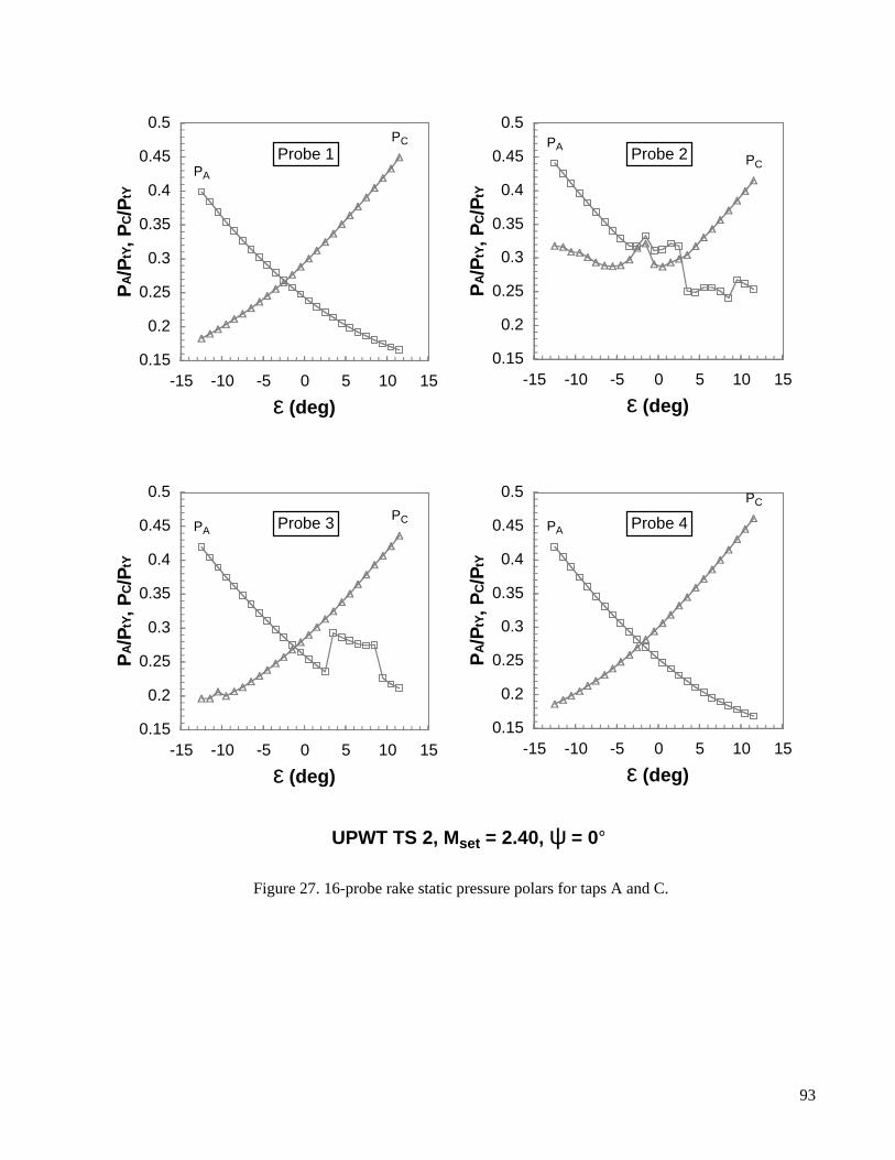
Figure 27. 16-probe rake static pressure polars for taps A and C.

PC

PA

0.15

0.2

0.25

0.3

0.35

0.4

0.45

0.5

-15 -10 -5 0 5 10 15

ε (deg)

PA/P

tY, P

C/P

tY

Probe 1 PC

PA

0.15

0.2

0.25

0.3

0.35

0.4

0.45

0.5

-15 -10 -5 0 5 10 15

ε (deg)

PA/P

tY, P

C/P

tY

Probe 2

PCPA

0.15

0.2

0.25

0.3

0.35

0.4

0.45

0.5

-15 -10 -5 0 5 10 15

ε (deg)

PA/P

tY, P

C/P

tY

Probe 3

PC

PA

0.15

0.2

0.25

0.3

0.35

0.4

0.45

0.5

-15 -10 -5 0 5 10 15

ε (deg)

PA/P

tY, P

C/P

tY

Probe 4

UPWT TS 2, Mset = 2.40, ψ = 0°

93

Figure 27. Continued.

PCPA

0.15

0.2

0.25

0.3

0.35

0.4

0.45

0.5

-15 -10 -5 0 5 10 15

ε (deg)

PA/P

tY, P

C/P

tY

Probe 5PC

PA

0.15

0.2

0.25

0.3

0.35

0.4

0.45

0.5

-15 -10 -5 0 5 10 15

ε (deg)

PA/P

tY, P

C/P

tY

Probe 6

PCPA

0.15

0.2

0.25

0.3

0.35

0.4

0.45

0.5

-15 -10 -5 0 5 10 15

ε (deg)

PA/P

tY, P

C/P

tY

Probe 7PC

PA

0.15

0.2

0.25

0.3

0.35

0.4

0.45

0.5

-15 -10 -5 0 5 10 15

ε (deg)

PA/P

tY, P

C/P

tY

Probe 8

UPWT TS 2, Mset = 2.40, ψ = 0°

94

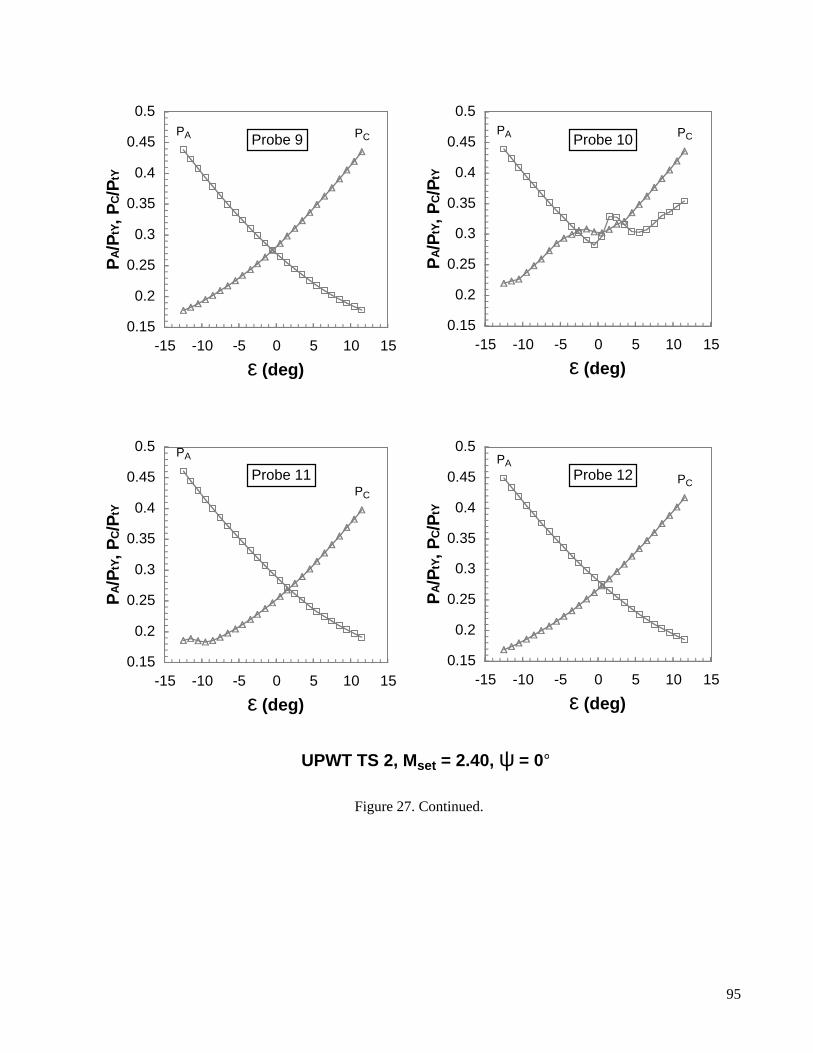
Figure 27. Continued.

PCPA

0.15

0.2

0.25

0.3

0.35

0.4

0.45

0.5

-15 -10 -5 0 5 10 15

ε (deg)

PA/P

tY, P

C/P

tY

Probe 9 PCPA

0.15

0.2

0.25

0.3

0.35

0.4

0.45

0.5

-15 -10 -5 0 5 10 15

ε (deg)

PA/P

tY, P

C/P

tY

Probe 10

PC

PA

0.15

0.2

0.25

0.3

0.35

0.4

0.45

0.5

-15 -10 -5 0 5 10 15

ε (deg)

PA/P

tY, P

C/P

tY

Probe 11 PC

PA

0.15

0.2

0.25

0.3

0.35

0.4

0.45

0.5

-15 -10 -5 0 5 10 15

ε (deg)

PA/P

tY, P

C/P

tY

Probe 12

UPWT TS 2, Mset = 2.40, ψ = 0°

95

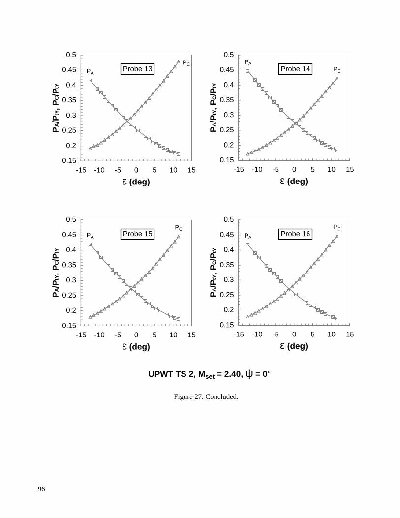
Figure 27. Concluded.

PC

PA

0.15

0.2

0.25

0.3

0.35

0.4

0.45

0.5

-15 -10 -5 0 5 10 15

ε (deg)

PA/P

tY, P

C/P

tY

Probe 13 PC

PA

0.15

0.2

0.25

0.3

0.35

0.4

0.45

0.5

-15 -10 -5 0 5 10 15

ε (deg)

PA/P

tY, P

C/P

tY

Probe 14

PCPA

0.15

0.2

0.25

0.3

0.35

0.4

0.45

0.5

-15 -10 -5 0 5 10 15

ε (deg)

PA/P

tY, P

C/P

tY

Probe 15PC

PA

0.15

0.2

0.25

0.3

0.35

0.4

0.45

0.5

-15 -10 -5 0 5 10 15

ε (deg)

PA/P

tY, P

C/P

tY

Probe 16

UPWT TS 2, Mset = 2.40, ψ = 0°

96

97

Probes Affected by Flow Disturbances

1 2 3 4

56 7

8

9 10

1112

13 14 15 16

Rake Body Channel Blockage

Figure 28. Location of affected probes relative to rake blockage areas.

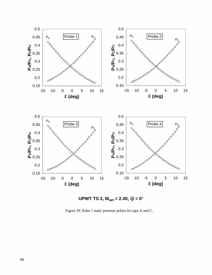
Figure 29. Rake 1 static pressure polars for taps A and C.

PA PC

0.15

0.2

0.25

0.3

0.35

0.4

0.45

0.5

-15 -10 -5 0 5 10 15

ε (deg)

PA/P

tY, P

C/P

tY

Probe 1 PAPC

0.15

0.2

0.25

0.3

0.35

0.4

0.45

0.5

-15 -10 -5 0 5 10 15

ε (deg)

PA/P

tY, P

C/P

tY

Probe 2

PA

PC

0.15

0.2

0.25

0.3

0.35

0.4

0.45

0.5

-15 -10 -5 0 5 10 15

ε (deg)

PA/P

tY, P

C/P

tY

Probe 3 PA PC

0.15

0.2

0.25

0.3

0.35

0.4

0.45

0.5

-15 -10 -5 0 5 10 15

ε (deg)

PA/P

tY, P

C/P

tY

Probe 4

UPWT TS 2, Mset = 2.40, ψ = 0°

98

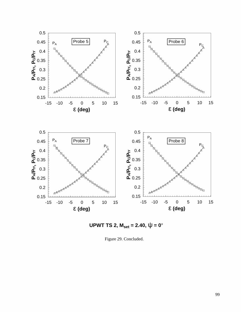
Figure 29. Concluded.

PAPC

0.15

0.2

0.25

0.3

0.35

0.4

0.45

0.5

-15 -10 -5 0 5 10 15

ε (deg)

PA/P

tY, P

C/P

tY

Probe 5 PAPC

0.15

0.2

0.25

0.3

0.35

0.4

0.45

0.5

-15 -10 -5 0 5 10 15

ε (deg)

PA/P

tY, P

C/P

tY

Probe 6

PA

PC

0.15

0.2

0.25

0.3

0.35

0.4

0.45

0.5

-15 -10 -5 0 5 10 15

ε (deg)

PA/P

tY, P

C/P

tY

Probe 7PA

PC

0.15

0.2

0.25

0.3

0.35

0.4

0.45

0.5

-15 -10 -5 0 5 10 15

ε (deg)

PA/P

tY, P

C/P

tY

Probe 8

UPWT TS 2, Mset = 2.40, ψ = 0°

99

Figure 30. Rake 2 static pressure polars for taps A and C.

PA

PC

0.15

0.2

0.25

0.3

0.35

0.4

0.45

0.5

-15 -10 -5 0 5 10 15

ε (deg)

PA/P

tY, P

C/P

tY

Probe 1PC

PA

0.15

0.2

0.25

0.3

0.35

0.4

0.45

0.5

-15 -10 -5 0 5 10 15

ε (deg)

PA/P

tY, P

C/P

tY

Probe 2

PCPA

0.15

0.2

0.25

0.3

0.35

0.4

0.45

0.5

-15 -10 -5 0 5 10 15

ε (deg)

PA/P

tY, P

C/P

tY

Probe 3

PC

PA

0.15

0.2

0.25

0.3

0.35

0.4

0.45

0.5

-15 -10 -5 0 5 10 15

ε (deg)

PA/P

tY, P

C/P

tY

Probe 4

UPWT TS 2, Mset = 2.40, ψ = 0°

100

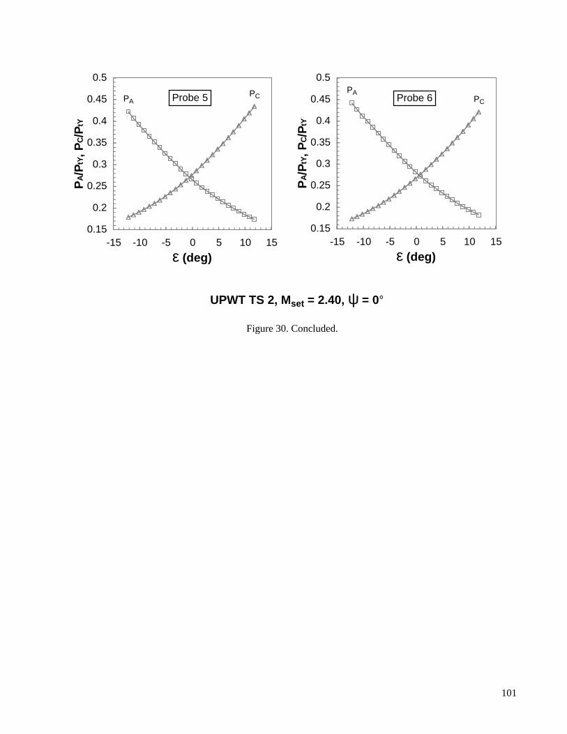
Figure 30. Concluded.

PAPC

0.15

0.2

0.25

0.3

0.35

0.4

0.45

0.5

-15 -10 -5 0 5 10 15

ε (deg)

PA/P

tY, P

C/P

tY

Probe 5 PC

PA

0.15

0.2

0.25

0.3

0.35

0.4

0.45

0.5

-15 -10 -5 0 5 10 15

ε (deg)

PA/P

tY, P

C/P

tY

Probe 6

UPWT TS 2, Mset = 2.40, ψ = 0°

101

102

16-Probe RakeMset = 2.15

8-Probe RakeMset = 2.40

6-Probe RakeMset = 2.29

Figure 31. Shadowgraph of cone-probe flow structure.

103

Figure 32. Cone-probe orientation angles.

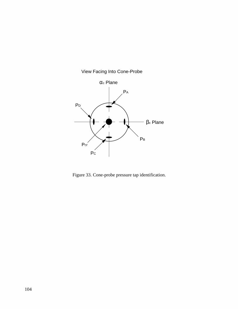
104

PA

PtY

αc Plane

βc Plane

PB

PC

PD

View Facing Into Cone-Probe

Figure 33. Cone-probe pressure tap identification.

Figure 34. Compressibility parameter variation with flow angle for rake 1.

Mset

2.15

2.29

2.40

0.26

0.265

0.27

0.275

0.28

0.285

0.29

0.295

0.3

0.305

0.31

0.315

0.32

-15 -10 -5 0 5 10 15

αC (deg)

PR

T

Nominal βC = 0°

Probe 1

Mset

2.15

2.29

2.40

0.26

0.265

0.27

0.275

0.28

0.285

0.29

0.295

0.3

0.305

0.31

0.315

0.32

-15 -10 -5 0 5 10 15

βC (deg)

PR

T

Nominal αC = 0°

105

Figure 34. Continued.

Mset

2.15

2.29

2.40

0.26

0.265

0.27

0.275

0.28

0.285

0.29

0.295

0.3

0.305

0.31

0.315

0.32

-15 -10 -5 0 5 10 15

αC (deg)

PR

T

Nominal βC = 0°

Probe 2

Mset

2.15

2.29

2.40

0.26

0.265

0.27

0.275

0.28

0.285

0.29

0.295

0.3

0.305

0.31

0.315

0.32

-15 -10 -5 0 5 10 15

βC (deg)

PR

T

Nominal αC = 0°

106

Figure 34. Continued.

Mset

2.15

2.29

2.40

0.26

0.265

0.27

0.275

0.28

0.285

0.29

0.295

0.3

0.305

0.31

0.315

0.32

-15 -10 -5 0 5 10 15

αC (deg)

PR

T

Nominal βC = 0°

Probe 3

Mset

2.15

2.29

2.40

0.26

0.265

0.27

0.275

0.28

0.285

0.29

0.295

0.3

0.305

0.31

0.315

0.32

-15 -10 -5 0 5 10 15

βC (deg)

PR

T

Nominal αC = 0°

107

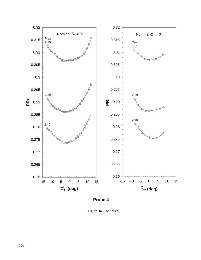
Figure 34. Continued.

Mset

2.15

2.29

2.40

0.26

0.265

0.27

0.275

0.28

0.285

0.29

0.295

0.3

0.305

0.31

0.315

0.32

-15 -10 -5 0 5 10 15

αC (deg)

PR

T

Nominal βC = 0°

Probe 4

Mset

2.15

2.29

2.40

0.26

0.265

0.27

0.275

0.28

0.285

0.29

0.295

0.3

0.305

0.31

0.315

0.32

-15 -10 -5 0 5 10 15

βC (deg)

PR

T

Nominal αC = 0°

108

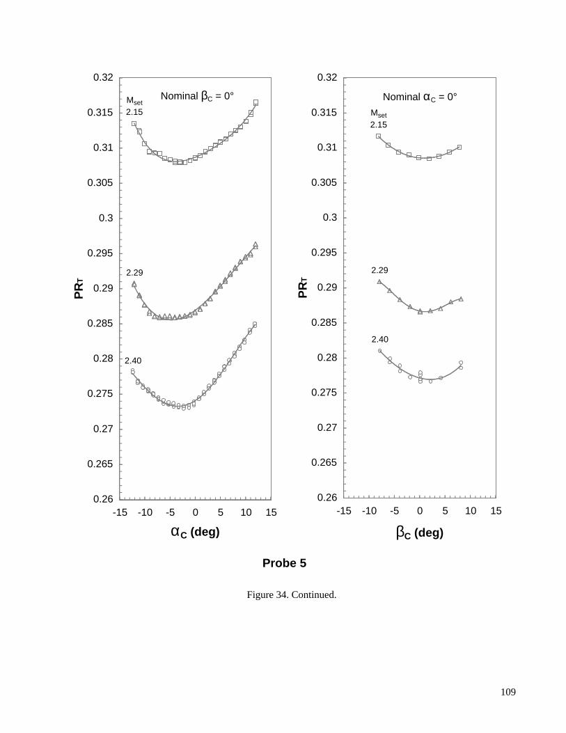
Figure 34. Continued.

Mset

2.15

2.29

2.40

0.26

0.265

0.27

0.275

0.28

0.285

0.29

0.295

0.3

0.305

0.31

0.315

0.32

-15 -10 -5 0 5 10 15

αC (deg)

PR

T

Nominal βC = 0°

Probe 5

Mset

2.15

2.29

2.40

0.26

0.265

0.27

0.275

0.28

0.285

0.29

0.295

0.3

0.305

0.31

0.315

0.32

-15 -10 -5 0 5 10 15

βC (deg)

PR

T

Nominal αC = 0°

109

Figure 34. Continued.

Mset

2.15

2.29

2.40

0.26

0.265

0.27

0.275

0.28

0.285

0.29

0.295

0.3

0.305

0.31

0.315

0.32

-15 -10 -5 0 5 10 15

αC (deg)

PR

T

Nominal βC = 0°

Probe 6

Mset

2.15

2.29

2.40

0.26

0.265

0.27

0.275

0.28

0.285

0.29

0.295

0.3

0.305

0.31

0.315

0.32

-15 -10 -5 0 5 10 15

βC (deg)

PR

T

Nominal αC = 0°

110

Figure 34. Continued.

Mset

2.15

2.29

2.40

0.26

0.265

0.27

0.275

0.28

0.285

0.29

0.295

0.3

0.305

0.31

0.315

0.32

-15 -10 -5 0 5 10 15

αC (deg)

PR

T

Nominal βC = 0°

Probe 7

Mset

2.15

2.29

2.40

0.26

0.265

0.27

0.275

0.28

0.285

0.29

0.295

0.3

0.305

0.31

0.315

0.32

-15 -10 -5 0 5 10 15

βC (deg)

PR

T

Nominal αC = 0°

111

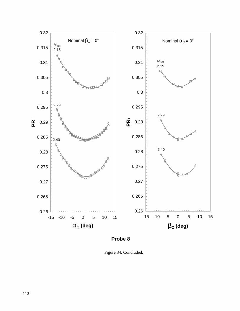
Figure 34. Concluded.

Mset

2.15

2.29

2.40

0.26

0.265

0.27

0.275

0.28

0.285

0.29

0.295

0.3

0.305

0.31

0.315

0.32

-15 -10 -5 0 5 10 15

αC (deg)

PR

T

Nominal βC = 0°

Probe 8

Mset

2.15

2.29

2.40

0.26

0.265

0.27

0.275

0.28

0.285

0.29

0.295

0.3

0.305

0.31

0.315

0.32

-15 -10 -5 0 5 10 15

βC (deg)

PR

T

Nominal αC = 0°

112

Figure 35. Compressibility parameter variation with flow angle for rake 2.

Mset

2.15

2.29

2.40

0.26

0.265

0.27

0.275

0.28

0.285

0.29

0.295

0.3

0.305

0.31

0.315

0.32

-15 -10 -5 0 5 10 15

αC (deg)

PR

T

Nominal βC = 0°

Probe 1

Mset

2.15

2.29

2.40

0.26

0.265

0.27

0.275

0.28

0.285

0.29

0.295

0.3

0.305

0.31

0.315

0.32

-15 -10 -5 0 5 10 15

βC (deg)

PR

T

Nominal αC = 0°

113

Figure 35. Continued.

Mset

2.15

2.29

2.40

0.27

0.275

0.28

0.285

0.29

0.295

0.3

0.305

0.31

0.315

0.32

0.325

0.33

-15 -10 -5 0 5 10 15

αC (deg)

PR

T

Nominal βC = 0°

Probe 2

Mset

2.15

2.29

2.40

0.27

0.275

0.28

0.285

0.29

0.295

0.3

0.305

0.31

0.315

0.32

0.325

0.33

-15 -10 -5 0 5 10 15

βC (deg)

PR

T

Nominal αC = 0°

114

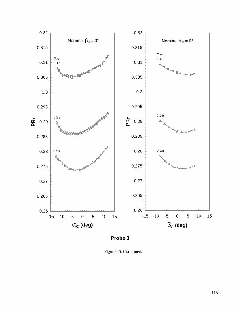
Figure 35. Continued.

Mset

2.15

2.29

2.40

0.26

0.265

0.27

0.275

0.28

0.285

0.29

0.295

0.3

0.305

0.31

0.315

0.32

-15 -10 -5 0 5 10 15

αC (deg)

PR

T

Nominal βC = 0°

Probe 3

Mset

2.15

2.29

2.40

0.26

0.265

0.27

0.275

0.28

0.285

0.29

0.295

0.3

0.305

0.31

0.315

0.32

-15 -10 -5 0 5 10 15

βC (deg)

PR

T

Nominal αC = 0°

115

Figure 35. Continued.

Mset

2.15

2.29

2.40

0.27

0.275

0.28

0.285

0.29

0.295

0.3

0.305

0.31

0.315

0.32

0.325

0.33

-15 -10 -5 0 5 10 15

αC (deg)

PR

T

Nominal βC = 0°

Probe 4

Mset

2.15

2.29

2.40

0.27

0.275

0.28

0.285

0.29

0.295

0.3

0.305

0.31

0.315

0.32

0.325

0.33

-15 -10 -5 0 5 10 15

βC (deg)

PR

T

Nominal αC = 0°

116

Figure 35. Continued.

Mset

2.15

2.29

2.40

0.26

0.265

0.27

0.275

0.28

0.285

0.29

0.295

0.3

0.305

0.31

0.315

0.32

-15 -10 -5 0 5 10 15

αC (deg)

PR

T

Nominal βC = 0°

Probe 5

Mset

2.15

2.29

2.40

0.26

0.265

0.27

0.275

0.28

0.285

0.29

0.295

0.3

0.305

0.31

0.315

0.32

-15 -10 -5 0 5 10 15

βC (deg)

PR

T

Nominal αC = 0°

117

Figure 35. Concluded.

Mset

2.15

2.29

2.40

0.26

0.265

0.27

0.275

0.28

0.285

0.29

0.295

0.3

0.305

0.31

0.315

0.32

-15 -10 -5 0 5 10 15

αC (deg)

PR

T

Nominal βC = 0°

Probe 6

Mset

2.15

2.29

2.40

0.26

0.265

0.27

0.275

0.28

0.285

0.29

0.295

0.3

0.305

0.31

0.315

0.32

-15 -10 -5 0 5 10 15

βC (deg)

PR

T

Nominal αC = 0°

118

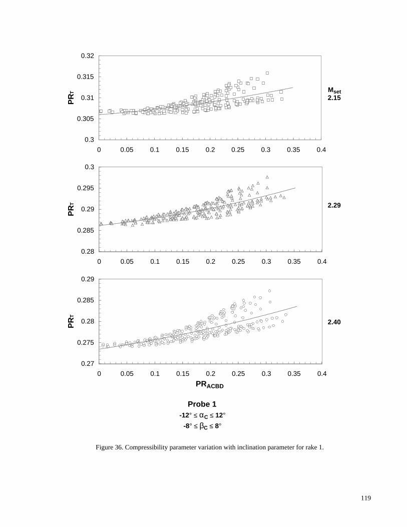
Figure 36. Compressibility parameter variation with inclination parameter for rake 1.

0.3

0.305

0.31

0.315

0.32

0 0.05 0.1 0.15 0.2 0.25 0.3 0.35 0.4

PR

T

0.28

0.285

0.29

0.295

0.3

0 0.05 0.1 0.15 0.2 0.25 0.3 0.35 0.4

PR

T

0.27

0.275

0.28

0.285

0.29

0 0.05 0.1 0.15 0.2 0.25 0.3 0.35 0.4

PRACBD

PR

T

Probe 1-12° ≤ αC ≤ 12°

-8° ≤ βC ≤ 8°

Mset2.15

2.29

2.40

119

Figure 36. Continued.

0.3

0.305

0.31

0.315

0.32

0 0.05 0.1 0.15 0.2 0.25 0.3 0.35 0.4

PR

T

0.28

0.285

0.29

0.295

0.3

0 0.05 0.1 0.15 0.2 0.25 0.3 0.35 0.4

PR

T

0.27

0.275

0.28

0.285

0.29

0 0.05 0.1 0.15 0.2 0.25 0.3 0.35 0.4

PRACBD

PR

T

Probe 2-12° ≤ αC ≤ 12°

-8° ≤ βC ≤ 8°

Mset2.15

2.29

2.40

120

Figure 36. Continued.

0.3

0.305

0.31

0.315

0.32

0 0.05 0.1 0.15 0.2 0.25 0.3 0.35 0.4

PR

T

0.28

0.285

0.29

0.295

0.3

0 0.05 0.1 0.15 0.2 0.25 0.3 0.35 0.4

PR

T

0.27

0.275

0.28

0.285

0.29

0 0.05 0.1 0.15 0.2 0.25 0.3 0.35 0.4

PRACBD

PR

T

Probe 3-12° ≤ αC ≤ 12°

-8° ≤ βC ≤ 8°

Mset2.15

2.29

2.40

121

Figure 36. Continued.

0.3

0.305

0.31

0.315

0.32

0 0.05 0.1 0.15 0.2 0.25 0.3 0.35 0.4

PR

T

0.28

0.285

0.29

0.295

0.3

0 0.05 0.1 0.15 0.2 0.25 0.3 0.35 0.4

PR

T

0.27

0.275

0.28

0.285

0.29

0 0.05 0.1 0.15 0.2 0.25 0.3 0.35 0.4

PRACBD

PR

T

Probe 4-12° ≤ αC ≤ 12°

-8° ≤ βC ≤ 8°

Mset2.15

2.29

2.40

122

Figure 36. Continued.

0.3

0.305

0.31

0.315

0.32

0 0.05 0.1 0.15 0.2 0.25 0.3 0.35 0.4

PR

T

0.28

0.285

0.29

0.295

0.3

0 0.05 0.1 0.15 0.2 0.25 0.3 0.35 0.4

PR

T

0.27

0.275

0.28

0.285

0.29

0 0.05 0.1 0.15 0.2 0.25 0.3 0.35 0.4

PRACBD

PR

T

Probe 5-12° ≤ αC ≤ 12°

-8° ≤ βC ≤ 8°

Mset2.15

2.29

2.40

123

Figure 36. Continued.

0.3

0.305

0.31

0.315

0.32

0 0.05 0.1 0.15 0.2 0.25 0.3 0.35 0.4

PR

T

0.28

0.285

0.29

0.295

0.3

0 0.05 0.1 0.15 0.2 0.25 0.3 0.35 0.4

PR

T

0.27

0.275

0.28

0.285

0.29

0 0.05 0.1 0.15 0.2 0.25 0.3 0.35 0.4

PRACBD

PR

T

Probe 6-12° ≤ αC ≤ 12°

-8° ≤ βC ≤ 8°

Mset2.15

2.29

2.40

124

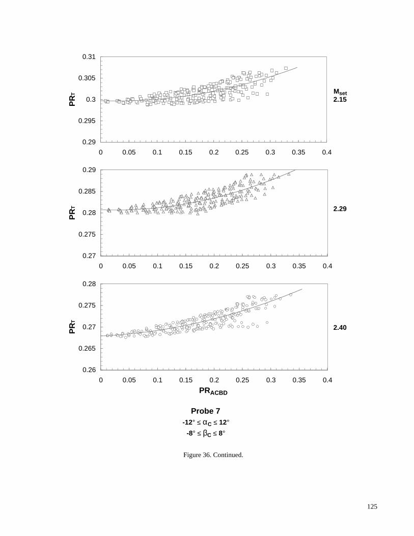
Figure 36. Continued.

0.29

0.295

0.3

0.305

0.31

0 0.05 0.1 0.15 0.2 0.25 0.3 0.35 0.4

PR

T

0.27

0.275

0.28

0.285

0.29

0 0.05 0.1 0.15 0.2 0.25 0.3 0.35 0.4

PR

T

0.26

0.265

0.27

0.275

0.28

0 0.05 0.1 0.15 0.2 0.25 0.3 0.35 0.4

PRACBD

PR

T

Probe 7-12° ≤ αC ≤ 12°

-8° ≤ βC ≤ 8°

Mset2.15

2.29

2.40

125

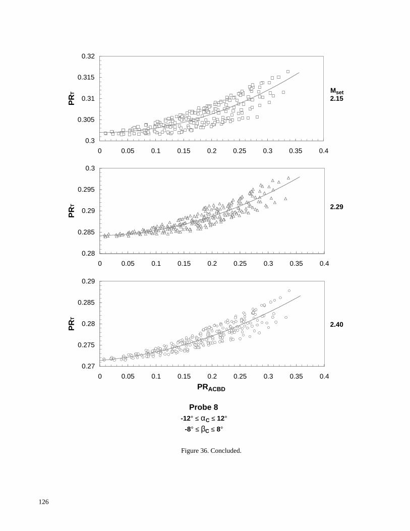
Figure 36. Concluded.

0.3

0.305

0.31

0.315

0.32

0 0.05 0.1 0.15 0.2 0.25 0.3 0.35 0.4

PR

T

0.28

0.285

0.29

0.295

0.3

0 0.05 0.1 0.15 0.2 0.25 0.3 0.35 0.4

PR

T

0.27

0.275

0.28

0.285

0.29

0 0.05 0.1 0.15 0.2 0.25 0.3 0.35 0.4

PRACBD

PR

T

Probe 8-12° ≤ αC ≤ 12°

-8° ≤ βC ≤ 8°

Mset2.15

2.29

2.40

126

Figure 37. Compressibility parameter variation with inclination parameter for rake 2.

0.3

0.305

0.31

0.315

0.32

0 0.05 0.1 0.15 0.2 0.25 0.3 0.35 0.4

PR

T

0.28

0.285

0.29

0.295

0.3

0 0.05 0.1 0.15 0.2 0.25 0.3 0.35 0.4

PR

T

0.27

0.275

0.28

0.285

0.29

0 0.05 0.1 0.15 0.2 0.25 0.3 0.35 0.4

PRACBD

PR

T

Probe 1-12° ≤ αC ≤ 12°

-8° ≤ βC ≤ 8°

Mset2.15

2.29

2.40

127

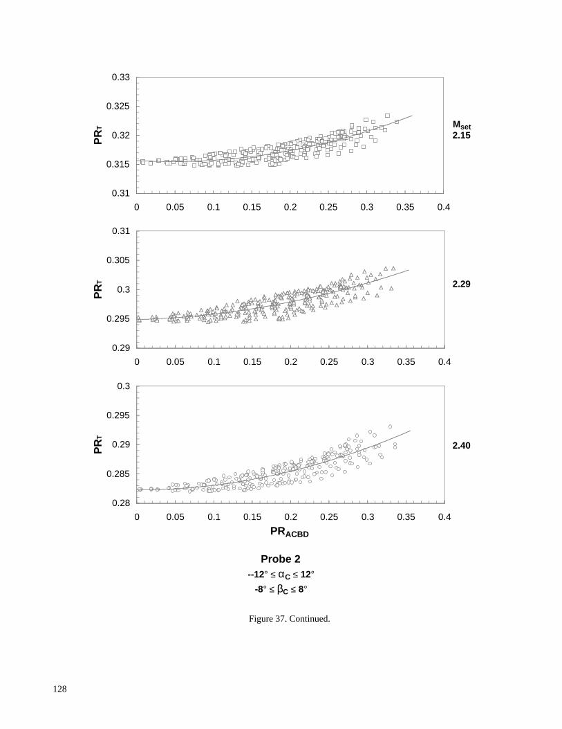
Figure 37. Continued.

0.31

0.315

0.32

0.325

0.33

0 0.05 0.1 0.15 0.2 0.25 0.3 0.35 0.4

PR

T

0.29

0.295

0.3

0.305

0.31

0 0.05 0.1 0.15 0.2 0.25 0.3 0.35 0.4

PR

T

0.28

0.285

0.29

0.295

0.3

0 0.05 0.1 0.15 0.2 0.25 0.3 0.35 0.4

PRACBD

PR

T

Probe 2--12° ≤ αC ≤ 12°

-8° ≤ βC ≤ 8°

Mset2.15

2.29

2.40

128

Figure 37. Continued.

0.3

0.305

0.31

0.315

0.32

0 0.05 0.1 0.15 0.2 0.25 0.3 0.35 0.4

PR

T

0.28

0.285

0.29

0.295

0.3

0 0.05 0.1 0.15 0.2 0.25 0.3 0.35 0.4

PR

T

0.27

0.275

0.28

0.285

0.29

0 0.05 0.1 0.15 0.2 0.25 0.3 0.35 0.4

PRACBD

PR

T

Probe 3-12° ≤ αC ≤ 12°

-8° ≤ βC ≤ 8°

Mset2.15

2.29

2.40

129

Figure 37. Continued.

0.31

0.315

0.32

0.325

0.33

0 0.05 0.1 0.15 0.2 0.25 0.3 0.35 0.4

PR

T

0.29

0.295

0.3

0.305

0.31

0 0.05 0.1 0.15 0.2 0.25 0.3 0.35 0.4

PR

T

0.28

0.285

0.29

0.295

0.3

0 0.05 0.1 0.15 0.2 0.25 0.3 0.35 0.4

PRACBD

PR

T

Probe 4-12° ≤ αC ≤ 12°

-8° ≤ βC ≤ 8°

Mset2.15

2.29

2.40

130

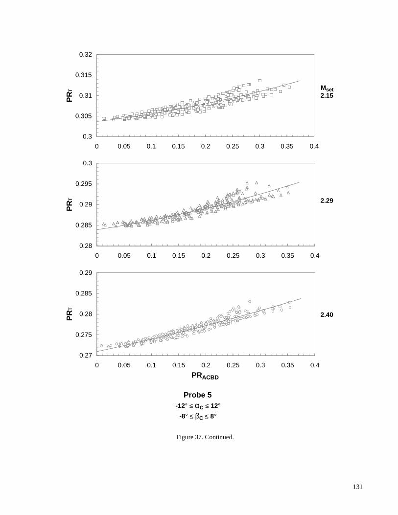
Figure 37. Continued.

0.3

0.305

0.31

0.315

0.32

0 0.05 0.1 0.15 0.2 0.25 0.3 0.35 0.4

PR

T

0.28

0.285

0.29

0.295

0.3

0 0.05 0.1 0.15 0.2 0.25 0.3 0.35 0.4

PR

T

0.27

0.275

0.28

0.285

0.29

0 0.05 0.1 0.15 0.2 0.25 0.3 0.35 0.4

PRACBD

PR

T

Probe 5-12° ≤ αC ≤ 12°

-8° ≤ βC ≤ 8°

Mset2.15

2.29

2.40

131

Figure 37. Concluded.

0.3

0.305

0.31

0.315

0.32

0 0.05 0.1 0.15 0.2 0.25 0.3 0.35 0.4

PR

T

0.28

0.285

0.29

0.295

0.3

0 0.05 0.1 0.15 0.2 0.25 0.3 0.35 0.4

PR

T

0.27

0.275

0.28

0.285

0.29

0 0.05 0.1 0.15 0.2 0.25 0.3 0.35 0.4

PRACBD

PR

T

Probe 6-12° ≤ αC ≤ 12°

-8° ≤ βC ≤ 8°

Mset2.15

2.29

2.40

132

Figure 38. Compressibility parameter variation with corrected inclination parameter for rake 1.

0.3

0.305

0.31

0.315

0.32

0 0.00002 0.00004 0.00006 0.00008 0.0001

PR

T

0.28

0.285

0.29

0.295

0.3

0 0.00002 0.00004 0.00006 0.00008 0.0001

PR

T

0.27

0.275

0.28

0.285

0.29

0 0.00002 0.00004 0.00006 0.00008 0.0001PRACBDcorrT

PR

T

Probe 1-8° ≤ αC, βC ≤ 8°

Mset2.15

2.29

2.40

133

Figure 38. Continued.

0.3

0.305

0.31

0.315

0.32

0 0.00002 0.00004 0.00006 0.00008 0.0001

PR

T

0.28

0.285

0.29

0.295

0.3

0 0.00002 0.00004 0.00006 0.00008 0.0001

PR

T

0.27

0.275

0.28

0.285

0.29

0 0.00002 0.00004 0.00006 0.00008 0.0001PRACBDcorrT

PR

T

Probe 2-8° ≤ αC, βC ≤ 8°

Mset2.15

2.29

2.40

134

Figure 38. Continued.

0.3

0.305

0.31

0.315

0.32

0 0.00002 0.00004 0.00006 0.00008 0.0001

PR

T

0.28

0.285

0.29

0.295

0.3

0 0.00002 0.00004 0.00006 0.00008 0.0001

PR

T

0.27

0.275

0.28

0.285

0.29

0 0.00002 0.00004 0.00006 0.00008 0.0001PRACBDcorrT

PR

T

Probe 3-8° ≤ αC, βC ≤ 8°

Mset2.15

2.29

2.40

135

Figure 38. Continued.

0.3

0.305

0.31

0.315

0.32

0 0.00002 0.00004 0.00006 0.00008 0.0001

PR

T

0.28

0.285

0.29

0.295

0.3

0 0.00002 0.00004 0.00006 0.00008 0.0001

PR

T

0.27

0.275

0.28

0.285

0.29

0 0.00002 0.00004 0.00006 0.00008 0.0001PRACBDcorrT

PR

T

Probe 4-8° ≤ αC, βC ≤ 8°

Mset2.15

2.29

2.40

136

Figure 38. Continued.

0.3

0.305

0.31

0.315

0.32

0 0.00002 0.00004 0.00006 0.00008 0.0001

PR

T

0.28

0.285

0.29

0.295

0.3

0 0.00002 0.00004 0.00006 0.00008 0.0001

PR

T

0.27

0.275

0.28

0.285

0.29

0 0.00002 0.00004 0.00006 0.00008 0.0001PRACBDcorrT

PR

T

Probe 5-8° ≤ αC, βC ≤ 8°

Mset2.15

2.29

2.40

137

Figure 38. Continued.

0.3

0.305

0.31

0.315

0.32

0 0.00002 0.00004 0.00006 0.00008 0.0001

PR

T

0.28

0.285

0.29

0.295

0.3

0 0.00002 0.00004 0.00006 0.00008 0.0001

PR

T

0.27

0.275

0.28

0.285

0.29

0 0.00002 0.00004 0.00006 0.00008 0.0001PRACBDcorrT

PR

T

Probe 6-8° ≤ αC, βC ≤ 8°

Mset2.15

2.29

2.40

138

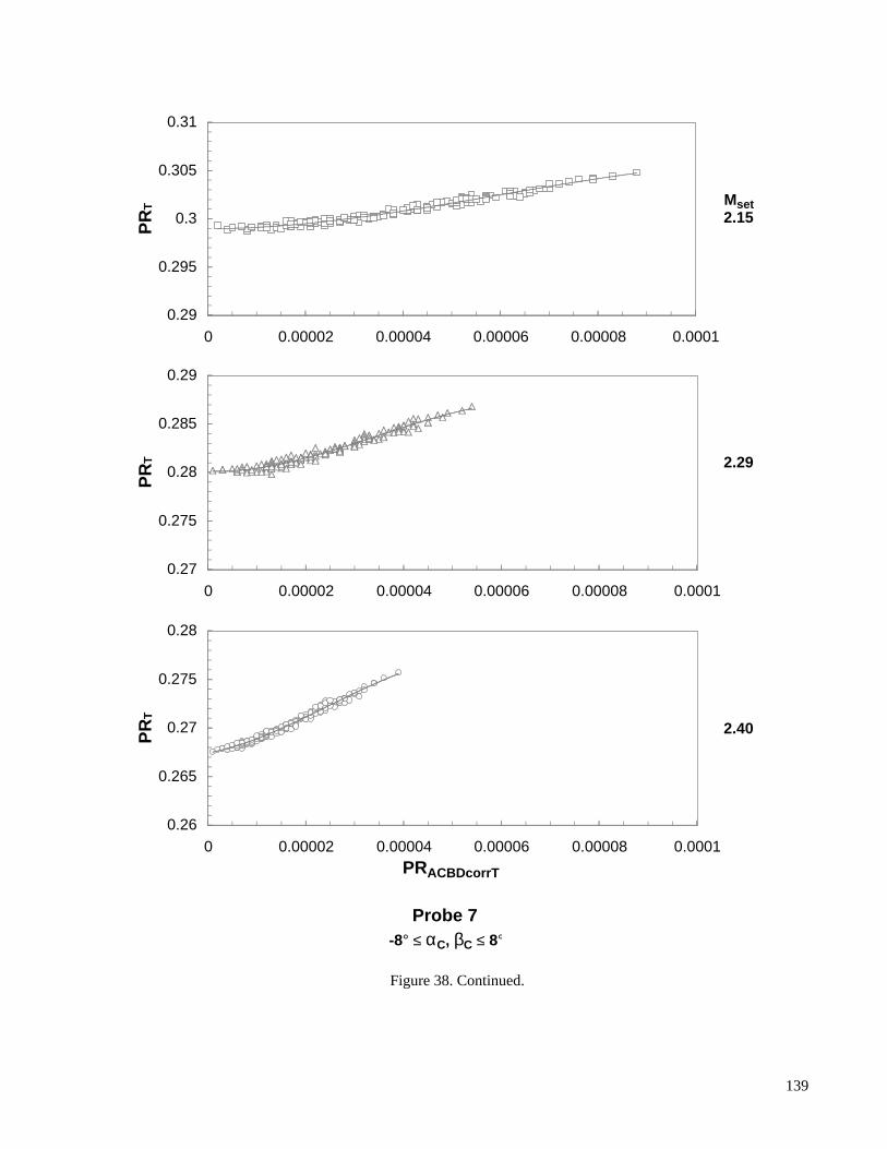
Figure 38. Continued.

0.29

0.295

0.3

0.305

0.31

0 0.00002 0.00004 0.00006 0.00008 0.0001

PR

T

0.27

0.275

0.28

0.285

0.29

0 0.00002 0.00004 0.00006 0.00008 0.0001

PR

T

0.26

0.265

0.27

0.275

0.28

0 0.00002 0.00004 0.00006 0.00008 0.0001PRACBDcorrT

PR

T

Probe 7-8° ≤ αC, βC ≤ 8°

Mset2.15

2.29

2.40

139

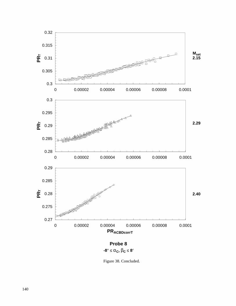
Figure 38. Concluded.

0.3

0.305

0.31

0.315

0.32

0 0.00002 0.00004 0.00006 0.00008 0.0001

PR

T

0.28

0.285

0.29

0.295

0.3

0 0.00002 0.00004 0.00006 0.00008 0.0001

PR

T

0.27

0.275

0.28

0.285

0.29

0 0.00002 0.00004 0.00006 0.00008 0.0001PRACBDcorrT

PR

T

Probe 8-8° ≤ αC, βC ≤ 8°

Mset2.15

2.29

2.40

140

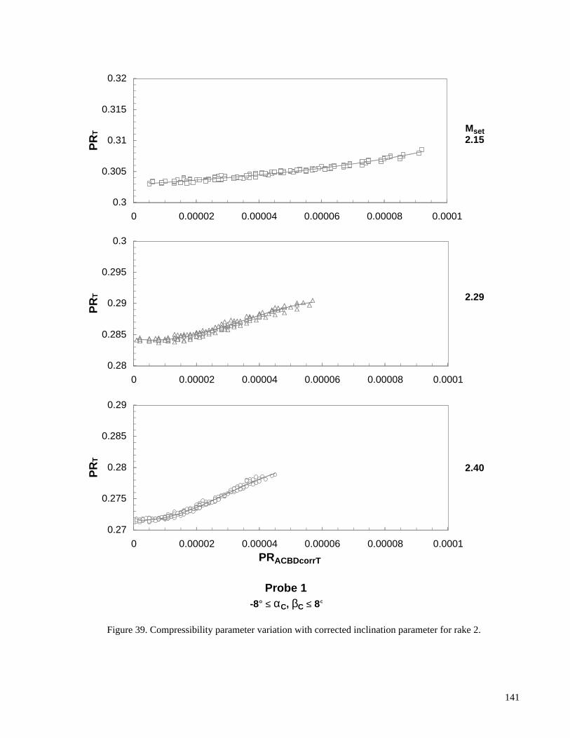
Figure 39. Compressibility parameter variation with corrected inclination parameter for rake 2.

0.3

0.305

0.31

0.315

0.32

0 0.00002 0.00004 0.00006 0.00008 0.0001

PR

T

0.28

0.285

0.29

0.295

0.3

0 0.00002 0.00004 0.00006 0.00008 0.0001

PR

T

0.27

0.275

0.28

0.285

0.29

0 0.00002 0.00004 0.00006 0.00008 0.0001PRACBDcorrT

PR

T

Probe 1-8° ≤ αC, βC ≤ 8°

Mset2.15

2.29

2.40

141

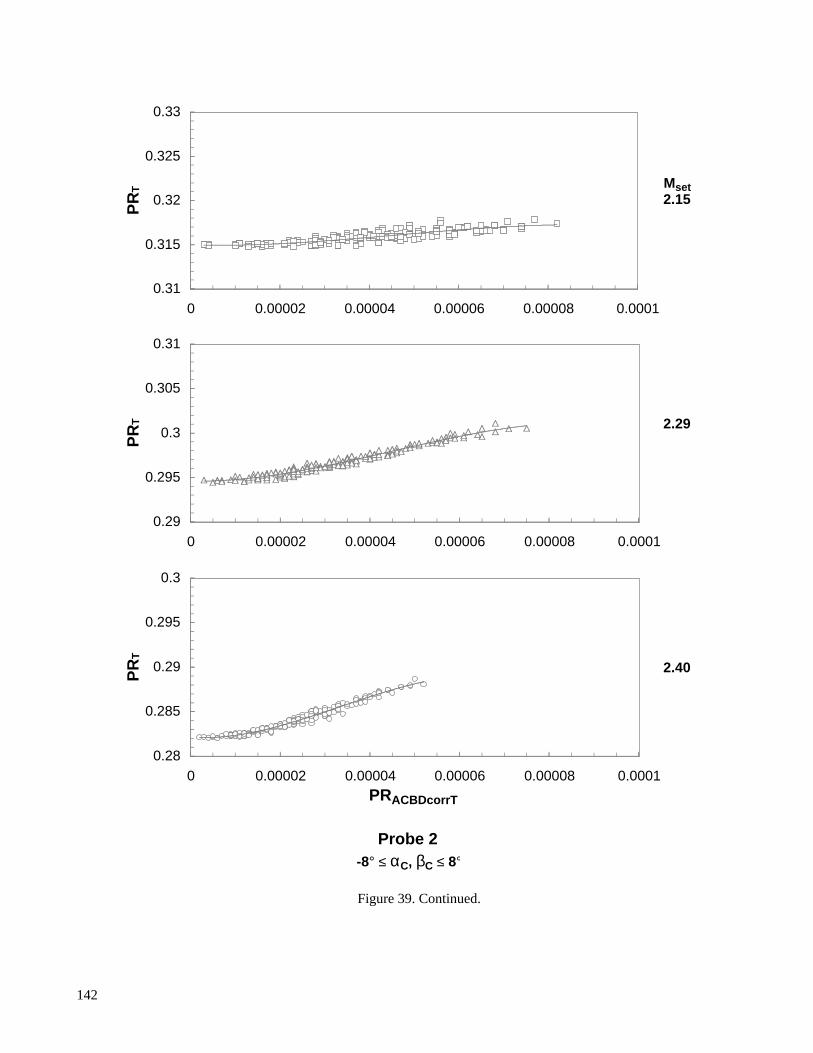
Figure 39. Continued.

0.31

0.315

0.32

0.325

0.33

0 0.00002 0.00004 0.00006 0.00008 0.0001

PR

T

0.29

0.295

0.3

0.305

0.31

0 0.00002 0.00004 0.00006 0.00008 0.0001

PR

T

0.28

0.285

0.29

0.295

0.3

0 0.00002 0.00004 0.00006 0.00008 0.0001PRACBDcorrT

PR

T

Probe 2-8° ≤ αC, βC ≤ 8°

Mset2.15

2.29

2.40

142

Figure 39. Continued.

0.3

0.305

0.31

0.315

0.32

0 0.00002 0.00004 0.00006 0.00008 0.0001

PR

T

0.28

0.285

0.29

0.295

0.3

0 0.00002 0.00004 0.00006 0.00008 0.0001

PR

T

0.27

0.275

0.28

0.285

0.29

0 0.00002 0.00004 0.00006 0.00008 0.0001PRACBDcorrT

PR

T

Probe 3-8° ≤ αC, βC ≤ 8°

Mset2.15

2.29

2.40

143

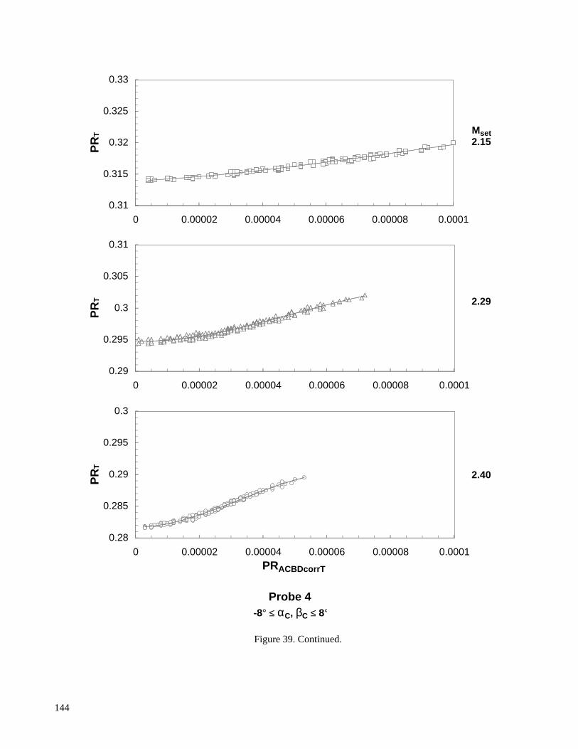
Figure 39. Continued.

0.31

0.315

0.32

0.325

0.33

0 0.00002 0.00004 0.00006 0.00008 0.0001

PR

T

0.29

0.295

0.3

0.305

0.31

0 0.00002 0.00004 0.00006 0.00008 0.0001

PR

T

0.28

0.285

0.29

0.295

0.3

0 0.00002 0.00004 0.00006 0.00008 0.0001PRACBDcorrT

PR

T

Probe 4-8° ≤ αC, βC ≤ 8°

Mset2.15

2.29

2.40

144

Figure 39. Continued.

0.3

0.305

0.31

0.315

0.32

0 0.00002 0.00004 0.00006 0.00008 0.0001

PR

T

0.28

0.285

0.29

0.295

0.3

0 0.00002 0.00004 0.00006 0.00008 0.0001

PR

T

0.27

0.275

0.28

0.285

0.29

0 0.00002 0.00004 0.00006 0.00008 0.0001PRACBDcorrT

PR

T

Probe 5-8° ≤ αC, βC ≤ 8°

Mset2.15

2.29

2.40

145

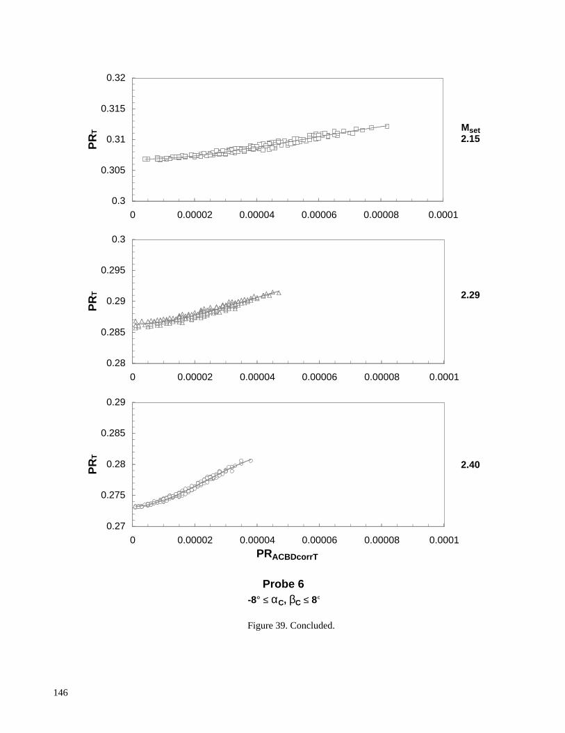
Figure 39. Concluded.

0.3

0.305

0.31

0.315

0.32

0 0.00002 0.00004 0.00006 0.00008 0.0001

PR

T

0.28

0.285

0.29

0.295

0.3

0 0.00002 0.00004 0.00006 0.00008 0.0001

PR

T

0.27

0.275

0.28

0.285

0.29

0 0.00002 0.00004 0.00006 0.00008 0.0001PRACBDcorrT

PR

T

Probe 6-8° ≤ αC, βC ≤ 8°

Mset2.15

2.29

2.40

146

147

Figure 40. Fundamental cone-probe compressibility parameter model.

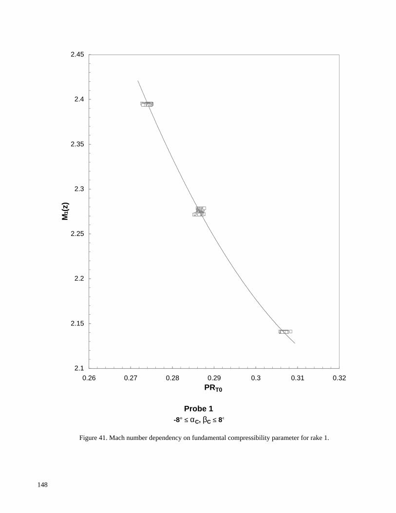
Figure 41. Mach number dependency on fundamental compressibility parameter for rake 1.

2.1

2.15

2.2

2.25

2.3

2.35

2.4

2.45

0.26 0.27 0.28 0.29 0.3 0.31 0.32PRT0

M1(

z)

Probe 1-8° ≤ αC, βC ≤ 8°

148

Figure 41. Continued.

2.1

2.15

2.2

2.25

2.3

2.35

2.4

2.45

0.26 0.27 0.28 0.29 0.3 0.31 0.32PRT0

M1(

z)

Probe 2-8° ≤ αC, βC ≤ 8°

149

Figure 41. Continued.

2.1

2.15

2.2

2.25

2.3

2.35

2.4

2.45

0.26 0.27 0.28 0.29 0.3 0.31 0.32PRT0

M1(

z)

Probe 3-8° ≤ αC, βC ≤ 8°

150

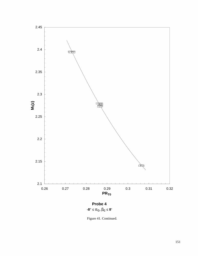
Figure 41. Continued.

2.1

2.15

2.2

2.25

2.3

2.35

2.4

2.45

0.26 0.27 0.28 0.29 0.3 0.31 0.32PRT0

M1(

z)

Probe 4-8° ≤ αC, βC ≤ 8°

151

Figure 41. Continued.

2.1

2.15

2.2

2.25

2.3

2.35

2.4

2.45

0.26 0.27 0.28 0.29 0.3 0.31 0.32PRT0

M1(

z)

Probe 5-8° ≤ αC, βC ≤ 8°

152

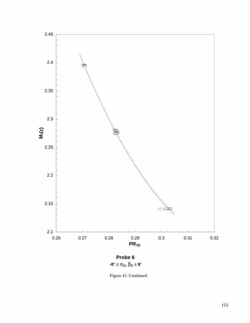
Figure 41. Continued.

2.1

2.15

2.2

2.25

2.3

2.35

2.4

2.45

0.26 0.27 0.28 0.29 0.3 0.31 0.32PRT0

M1(

z)

Probe 6-8° ≤ αC, βC ≤ 8°

153

Figure 41. Continued.

2.1

2.15

2.2

2.25

2.3

2.35

2.4

2.45

0.26 0.27 0.28 0.29 0.3 0.31 0.32PRT0

M1(

z)

Probe 7-8° ≤ αC, βC ≤ 8°

154

Figure 41. Concluded.

2.1

2.15

2.2

2.25

2.3

2.35

2.4

2.45

0.26 0.27 0.28 0.29 0.3 0.31 0.32PRT0

M1(

z)

Probe 8-8° ≤ αC, βC ≤ 8°

155

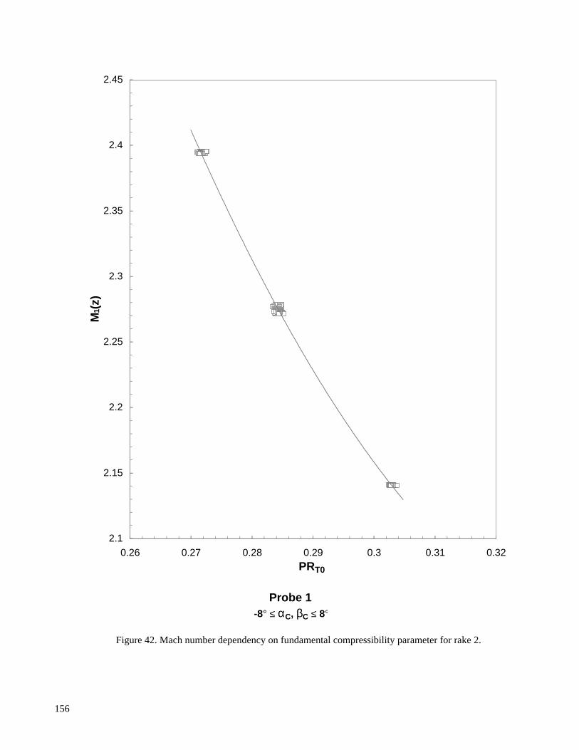
Figure 42. Mach number dependency on fundamental compressibility parameter for rake 2.

2.1

2.15

2.2

2.25

2.3

2.35

2.4

2.45

0.26 0.27 0.28 0.29 0.3 0.31 0.32PRT0

M1(

z)

Probe 1-8° ≤ αC, βC ≤ 8°

156

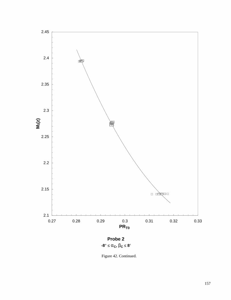
Figure 42. Continued.

2.1

2.15

2.2

2.25

2.3

2.35

2.4

2.45

0.27 0.28 0.29 0.3 0.31 0.32 0.33PRT0

M1(

z)

Probe 2-8° ≤ αC, βC ≤ 8°

157

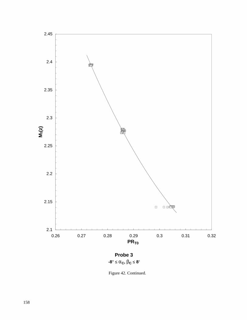
Figure 42. Continued.

2.1

2.15

2.2

2.25

2.3

2.35

2.4

2.45

0.26 0.27 0.28 0.29 0.3 0.31 0.32PRT0

M1(

z)

Probe 3-8° ≤ αC, βC ≤ 8°

158

Figure 42. Continued.

2.1

2.15

2.2

2.25

2.3

2.35

2.4

2.45

0.27 0.28 0.29 0.3 0.31 0.32 0.33PRT0

M1(

z)

Probe 4-8° ≤ αC, βC ≤ 8°

159

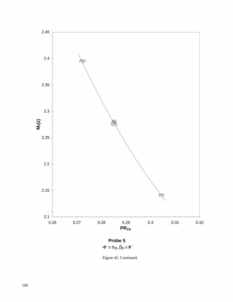
Figure 42. Continued.

2.1

2.15

2.2

2.25

2.3

2.35

2.4

2.45

0.26 0.27 0.28 0.29 0.3 0.31 0.32PRT0

M1(

z)

Probe 5-8° ≤ αC, βC ≤ 8°

160

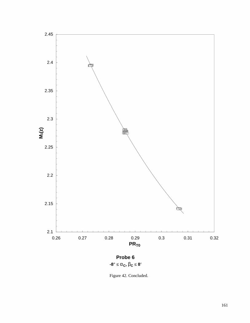
Figure 42. Concluded.

2.1

2.15

2.2

2.25

2.3

2.35

2.4

2.45

0.26 0.27 0.28 0.29 0.3 0.31 0.32PRT0

M1(

z)

Probe 6-8° ≤ αC, βC ≤ 8°

161

Figure 43. Mach number correlation residual for rake 1.

0

0.005

0.01

0.015

0.02

2.1 2.15 2.2 2.25 2.3 2.35 2.4

Average M1Ccal

±2σ(

M1C

cal)

Probe 1

0

0.005

0.01

0.015

0.02

2.1 2.15 2.2 2.25 2.3 2.35 2.4

Average M1Ccal

±2σ(

M1C

cal)

Probe 2

0

0.005

0.01

0.015

0.02

2.1 2.15 2.2 2.25 2.3 2.35 2.4

Average M1Ccal

±2σ(

M1C

cal)

Probe 3

0

0.005

0.01

0.015

0.02

2.1 2.15 2.2 2.25 2.3 2.35 2.4

Average M1Ccal

±2σ(

M1C

cal)

±4°/±4°±4°/±8°±8°/±4°±8°/±8°

Probe 4

αC/βC Range

162

Figure 43. Concluded.

0

0.005

0.01

0.015

0.02

2.1 2.15 2.2 2.25 2.3 2.35 2.4

Average M1Ccal

±2σ(

M1C

cal)

Probe 5

0

0.005

0.01

0.015

0.02

2.1 2.15 2.2 2.25 2.3 2.35 2.4

Average M1Ccal

±2σ(

M1C

cal)

Probe 6

0

0.005

0.01

0.015

0.02

2.1 2.15 2.2 2.25 2.3 2.35 2.4

Average M1Ccal

±2σ(

M1C

cal)

Probe 7

0

0.005

0.01

0.015

0.02

2.1 2.15 2.2 2.25 2.3 2.35 2.4

Average M1Ccal

±2σ(

M1C

cal)

±4°/±4°±4°/±8°±8°/±4°±8°/±8°

Probe 8

αC/βC Range

163

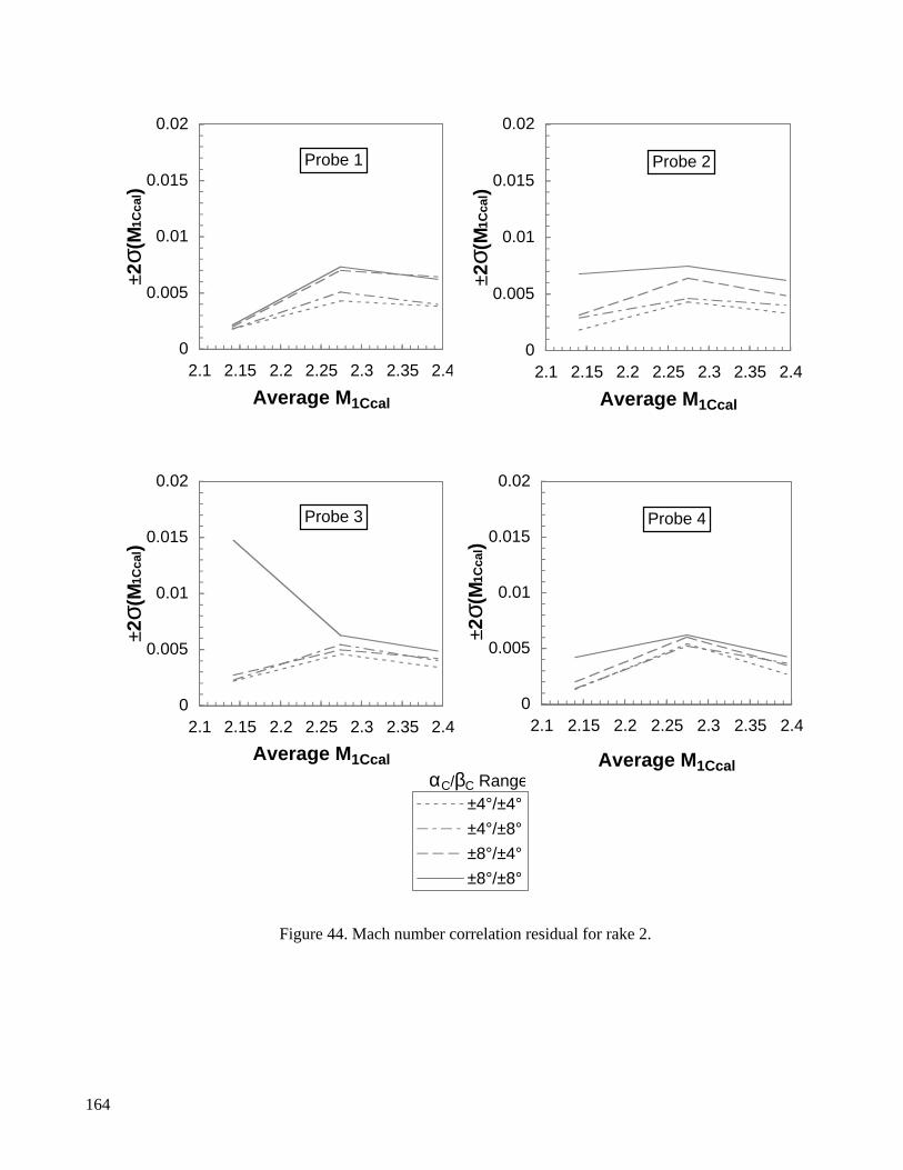
Figure 44. Mach number correlation residual for rake 2.

0

0.005

0.01

0.015

0.02

2.1 2.15 2.2 2.25 2.3 2.35 2.4

Average M1Ccal

±2σ(

M1C

cal)

Probe 1

0

0.005

0.01

0.015

0.02

2.1 2.15 2.2 2.25 2.3 2.35 2.4

Average M1Ccal

±2σ(

M1C

cal)

Probe 2

0

0.005

0.01

0.015

0.02

2.1 2.15 2.2 2.25 2.3 2.35 2.4

Average M1Ccal

±2σ(

M1C

cal)

Probe 3

0

0.005

0.01

0.015

0.02

2.1 2.15 2.2 2.25 2.3 2.35 2.4

Average M1Ccal

±2σ(

M1C

cal)

±4°/±4°±4°/±8°±8°/±4°±8°/±8°

Probe 4

αC/βC Range

164

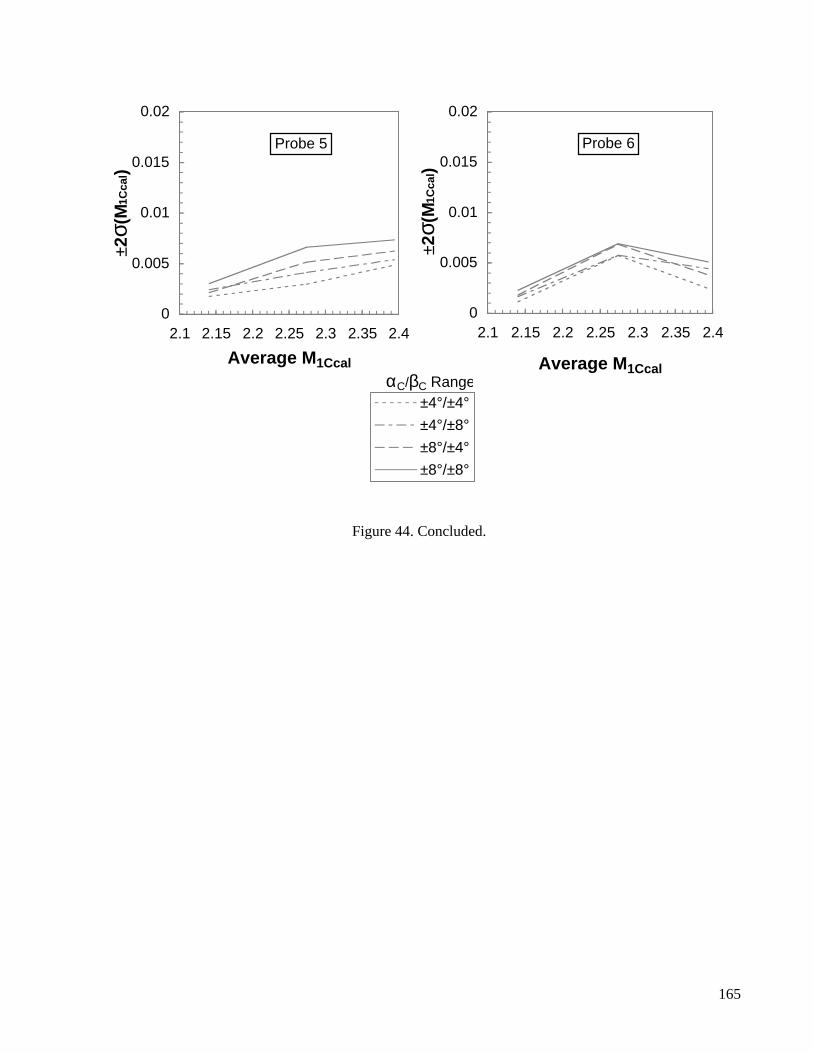
Figure 44. Concluded.

0

0.005

0.01

0.015

0.02

2.1 2.15 2.2 2.25 2.3 2.35 2.4

Average M1Ccal

±2σ(

M1C

cal)

Probe 5

0

0.005

0.01

0.015

0.02

2.1 2.15 2.2 2.25 2.3 2.35 2.4

Average M1Ccal

±2σ(

M1C

cal)

±4°/±4°±4°/±8°±8°/±4°±8°/±8°

Probe 6

αC/βC Range

165

Figure 45. Pitot pressure variation with flow angle for rake 1.

Mset

2.15

2.29

2.40

0.52

0.53

0.54

0.55

0.56

0.57

0.58

0.59

0.6

0.61

0.62

0.63

0.64

0.65

0.66

-15 -10 -5 0 5 10 15

αC (deg)

Pty/P

t0

Nominal βC = 0°

Probe 1

Mset

2.15

2.29

2.40

0.52

0.53

0.54

0.55

0.56

0.57

0.58

0.59

0.6

0.61

0.62

0.63

0.64

0.65

0.66

-15 -10 -5 0 5 10 15

βC (deg)

Pty/P

t0

Nominal αC = 0°

166

Figure 45. Continued.

Mset

2.15

2.29

2.40

0.52

0.53

0.54

0.55

0.56

0.57

0.58

0.59

0.6

0.61

0.62

0.63

0.64

0.65

0.66

-15 -10 -5 0 5 10 15

αC (deg)

Pty/P

t0

Nominal βC = 0°

Probe 2

Mset

2.15

2.29

2.40

0.52

0.53

0.54

0.55

0.56

0.57

0.58

0.59

0.6

0.61

0.62

0.63

0.64

0.65

0.66

-15 -10 -5 0 5 10 15

βC (deg)

Pty/P

t0

Nominal αC = 0°

167

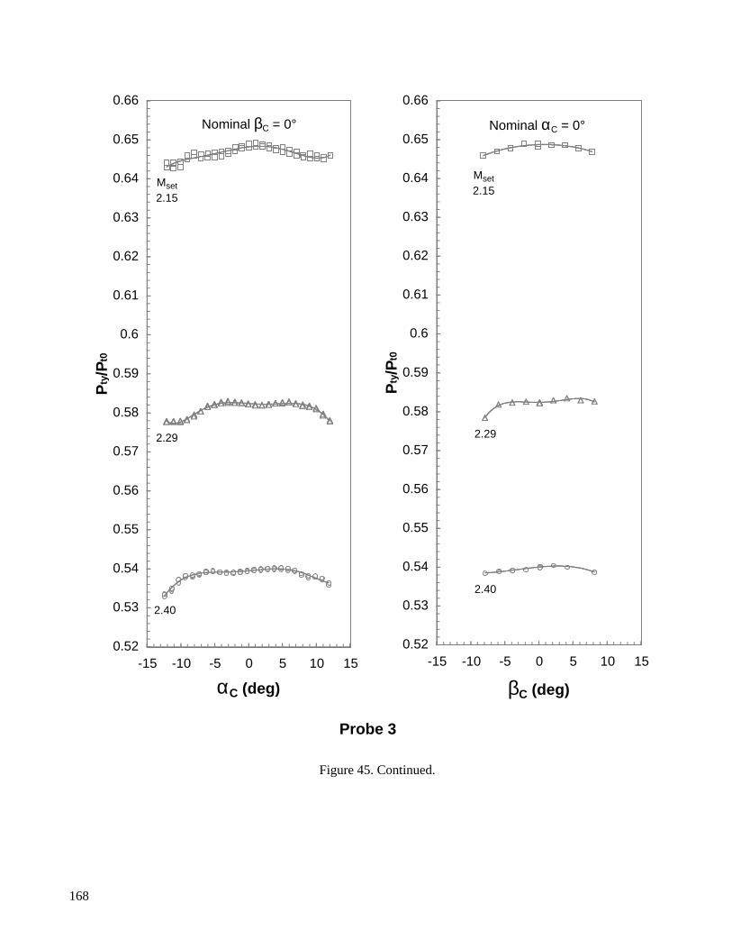
Figure 45. Continued.

Mset

2.15

2.29

2.40

0.52

0.53

0.54

0.55

0.56

0.57

0.58

0.59

0.6

0.61

0.62

0.63

0.64

0.65

0.66

-15 -10 -5 0 5 10 15

αC (deg)

Pty/P

t0

Nominal βC = 0°

Probe 3

Mset

2.15

2.29

2.40

0.52

0.53

0.54

0.55

0.56

0.57

0.58

0.59

0.6

0.61

0.62

0.63

0.64

0.65

0.66

-15 -10 -5 0 5 10 15

βC (deg)

Pty/P

t0

Nominal αC = 0°

168

Figure 45. Continued.

Mset

2.15

2.29

2.40

0.52

0.53

0.54

0.55

0.56

0.57

0.58

0.59

0.6

0.61

0.62

0.63

0.64

0.65

0.66

-15 -10 -5 0 5 10 15

αC (deg)

Pty/P

t0

Nominal βC = 0°

Probe 4

Mset

2.15

2.29

2.40

0.52

0.53

0.54

0.55

0.56

0.57

0.58

0.59

0.6

0.61

0.62

0.63

0.64

0.65

0.66

-15 -10 -5 0 5 10 15

βC (deg)

Pty/P

t0

Nominal αC = 0°

169

Figure 45. Continued.

Mset

2.15

2.29

2.40

0.52

0.53

0.54

0.55

0.56

0.57

0.58

0.59

0.6

0.61

0.62

0.63

0.64

0.65

0.66

-15 -10 -5 0 5 10 15

αC (deg)

Pty/P

t0

Nominal βC = 0°

Probe 5

Mset

2.15

2.29

2.40

0.52

0.53

0.54

0.55

0.56

0.57

0.58

0.59

0.6

0.61

0.62

0.63

0.64

0.65

0.66

-15 -10 -5 0 5 10 15

βC (deg)

Pty/P

t0

Nominal αC = 0°

170

Figure 45. Continued.

Mset

2.15

2.29

2.40

0.52

0.53

0.54

0.55

0.56

0.57

0.58

0.59

0.6

0.61

0.62

0.63

0.64

0.65

0.66

-15 -10 -5 0 5 10 15

αC (deg)

Pty/P

t0

Nominal βC = 0°

Probe 6

Mset

2.15

2.29

2.40

0.52

0.53

0.54

0.55

0.56

0.57

0.58

0.59

0.6

0.61

0.62

0.63

0.64

0.65

0.66

-15 -10 -5 0 5 10 15

βC (deg)

Pty/P

t0

Nominal αC = 0°

171

Figure 45. Continued.

Mset

2.15

2.29

2.40

0.52

0.53

0.54

0.55

0.56

0.57

0.58

0.59

0.6

0.61

0.62

0.63

0.64

0.65

0.66

-15 -10 -5 0 5 10 15

αC (deg)

Pty/P

t0

Nominal βC = 0°

Probe 7

Mset

2.15

2.29

2.40

0.52

0.53

0.54

0.55

0.56

0.57

0.58

0.59

0.6

0.61

0.62

0.63

0.64

0.65

0.66

-15 -10 -5 0 5 10 15

βC (deg)

Pty/P

t0

Nominal αC = 0°

172

Figure 45. Concluded.

Mset

2.15

2.29

2.40

0.52

0.53

0.54

0.55

0.56

0.57

0.58

0.59

0.6

0.61

0.62

0.63

0.64

0.65

0.66

-15 -10 -5 0 5 10 15

αC (deg)

Pty/P

t0

Nominal βC = 0°

Probe 8

Mset

2.15

2.29

2.40

0.52

0.53

0.54

0.55

0.56

0.57

0.58

0.59

0.6

0.61

0.62

0.63

0.64

0.65

0.66

-15 -10 -5 0 5 10 15

βC (deg)

Pty/P

t0

Nominal αC = 0°

173

Figure 46. Pitot pressure variation with flow angle for rake 2.

Mset

2.15

2.29

2.40

0.52

0.53

0.54

0.55

0.56

0.57

0.58

0.59

0.6

0.61

0.62

0.63

0.64

0.65

0.66

-15 -10 -5 0 5 10 15

αC (deg)

Pty/P

t0

Nominal βC = 0°

Probe 1

Mset

2.15

2.29

2.40

0.52

0.53

0.54

0.55

0.56

0.57

0.58

0.59

0.6

0.61

0.62

0.63

0.64

0.65

0.66

-15 -10 -5 0 5 10 15

βC (deg)

Pty/P

t0

Nominal αC = 0°

174

Figure 46. Continued.

Mset

2.15

2.29

2.40

0.52

0.53

0.54

0.55

0.56

0.57

0.58

0.59

0.6

0.61

0.62

0.63

0.64

0.65

0.66

-15 -10 -5 0 5 10 15

αC (deg)

Pty/P

t0

Nominal βC = 0°

Probe 2

Mset

2.15

2.29

2.40

0.52

0.53

0.54

0.55

0.56

0.57

0.58

0.59

0.6

0.61

0.62

0.63

0.64

0.65

0.66

-15 -10 -5 0 5 10 15

βC (deg)

Pty/P

t0

Nominal αC = 0°

175

Figure 46. Continued.

Mset

2.15

2.29

2.40

0.52

0.53

0.54

0.55

0.56

0.57

0.58

0.59

0.6

0.61

0.62

0.63

0.64

0.65

0.66

-15 -10 -5 0 5 10 15

αC (deg)

Pty/P

t0

Nominal βC = 0°

Probe 3

Mset

2.15

2.29

2.40

0.52

0.53

0.54

0.55

0.56

0.57

0.58

0.59

0.6

0.61

0.62

0.63

0.64

0.65

0.66

-15 -10 -5 0 5 10 15

βC (deg)

Pty/P

t0

Nominal αC = 0°

176

Figure 46. Continued.

Mset

2.15

2.29

2.40

0.52

0.53

0.54

0.55

0.56

0.57

0.58

0.59

0.6

0.61

0.62

0.63

0.64

0.65

0.66

-15 -10 -5 0 5 10 15

αC (deg)

Pty/P

t0

Nominal βC = 0°

Probe 4

Mset

2.15

2.29

2.40

0.52

0.53

0.54

0.55

0.56

0.57

0.58

0.59

0.6

0.61

0.62

0.63

0.64

0.65

0.66

-15 -10 -5 0 5 10 15

βC (deg)

Pty/P

t0

Nominal αC = 0°

177

Figure 46. Continued.

Mset

2.15

2.29

2.40

0.52

0.53

0.54

0.55

0.56

0.57

0.58

0.59

0.6

0.61

0.62

0.63

0.64

0.65

0.66

-15 -10 -5 0 5 10 15

αC (deg)

Pty/P

t0

Nominal βC = 0°

Probe 5

Mset

2.15

2.29

2.40

0.52

0.53

0.54

0.55

0.56

0.57

0.58

0.59

0.6

0.61

0.62

0.63

0.64

0.65

0.66

-15 -10 -5 0 5 10 15

βC (deg)

Pty/P

t0

Nominal αC = 0°

178

Figure 46. Concluded.

Mset

2.15

2.29

2.40

0.52

0.53

0.54

0.55

0.56

0.57

0.58

0.59

0.6

0.61

0.62

0.63

0.64

0.65

0.66

-15 -10 -5 0 5 10 15

αC (deg)

Pty/P

t0

Nominal βC = 0°

Probe 6

Mset

2.15

2.29

2.40

0.52

0.53

0.54

0.55

0.56

0.57

0.58

0.59

0.6

0.61

0.62

0.63

0.64

0.65

0.66

-15 -10 -5 0 5 10 15

βC (deg)

Pty/P

t0

Nominal αC = 0°

179

Figure 47. Pitot pressure variation with inclination parameter for rake 1.

0.635

0.64

0.645

0.65

0.655

0 0.05 0.1 0.15 0.2 0.25 0.3 0.35 0.4

Pty/P

t0

0.565

0.57

0.575

0.58

0.585

0 0.05 0.1 0.15 0.2 0.25 0.3 0.35 0.4

Pty/P

t0

0.525

0.53

0.535

0.54

0.545

0 0.05 0.1 0.15 0.2 0.25 0.3 0.35 0.4PRACBD

Pty/P

t0

Probe 1-8° ≤ αC, βC ≤ 8°

Mset2.15

2.29

2.40

180

Figure 47. Continued.

0.64

0.645

0.65

0.655

0.66

0 0.05 0.1 0.15 0.2 0.25 0.3 0.35 0.4

Pty/P

t0

0.57

0.575

0.58

0.585

0.59

0 0.05 0.1 0.15 0.2 0.25 0.3 0.35 0.4

Pty/P

t0

0.53

0.535

0.54

0.545

0.55

0 0.05 0.1 0.15 0.2 0.25 0.3 0.35 0.4PRACBD

Pty/P

t0

Probe 2-8° ≤ αC, βC ≤ 8°

Mset2.15

2.29

2.40

181

Figure 47. Continued.

0.64

0.645

0.65

0.655

0.66

0 0.05 0.1 0.15 0.2 0.25 0.3 0.35 0.4

Pty/P

t0

0.57

0.575

0.58

0.585

0.59

0 0.05 0.1 0.15 0.2 0.25 0.3 0.35 0.4

Pty/P

t0

0.53

0.535

0.54

0.545

0.55

0 0.05 0.1 0.15 0.2 0.25 0.3 0.35 0.4PRACBD

Pty/P

t0

Probe 3-8° ≤ αC, βC ≤ 8°

Mset2.15

2.29

2.40

182

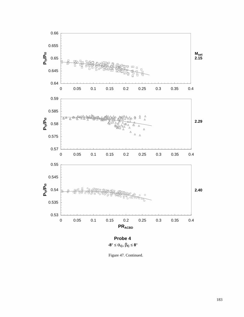
Figure 47. Continued.

0.64

0.645

0.65

0.655

0.66

0 0.05 0.1 0.15 0.2 0.25 0.3 0.35 0.4

Pty

/Pt0

0.57

0.575

0.58

0.585

0.59

0 0.05 0.1 0.15 0.2 0.25 0.3 0.35 0.4

Pty

/Pt0

0.53

0.535

0.54

0.545

0.55

0 0.05 0.1 0.15 0.2 0.25 0.3 0.35 0.4

PRACBD

Pty

/Pt0

Probe 4-8° ≤ αC, βC ≤ 8°

Mset2.15

2.29

2.40

183

Figure 47. Continued.

0.635

0.64

0.645

0.65

0.655

0 0.05 0.1 0.15 0.2 0.25 0.3 0.35 0.4

Pty/P

t0

0.57

0.575

0.58

0.585

0.59

0 0.05 0.1 0.15 0.2 0.25 0.3 0.35 0.4

Pty/P

t0

0.53

0.535

0.54

0.545

0.55

0 0.05 0.1 0.15 0.2 0.25 0.3 0.35 0.4PRACBD

Pty/P

t0

Probe 5-8° ≤ αC, βC ≤ 8°

Mset2.15

2.29

2.40

184

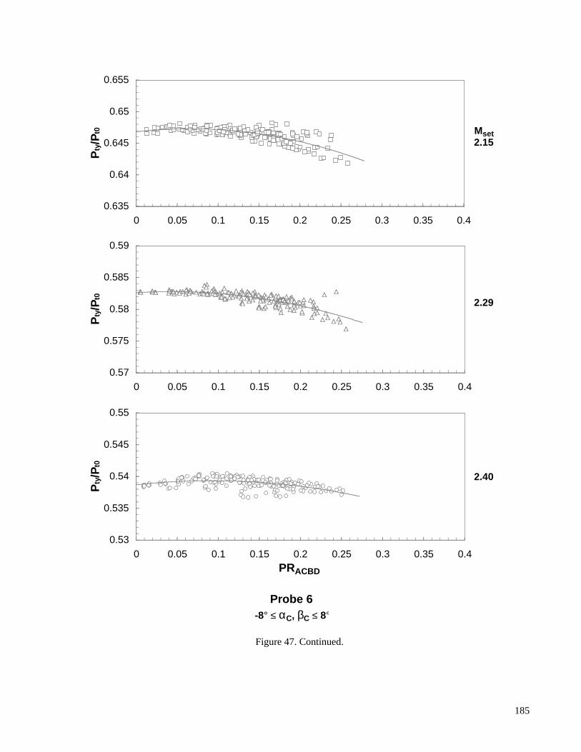
Figure 47. Continued.

0.635

0.64

0.645

0.65

0.655

0 0.05 0.1 0.15 0.2 0.25 0.3 0.35 0.4

Pty/P

t0

0.57

0.575

0.58

0.585

0.59

0 0.05 0.1 0.15 0.2 0.25 0.3 0.35 0.4

Pty/P

t0

0.53

0.535

0.54

0.545

0.55

0 0.05 0.1 0.15 0.2 0.25 0.3 0.35 0.4PRACBD

Pty/P

t0

Probe 6-8° ≤ αC, βC ≤ 8°

Mset2.15

2.29

2.40

185

Figure 47. Continued.

0.635

0.64

0.645

0.65

0.655

0 0.05 0.1 0.15 0.2 0.25 0.3 0.35 0.4

Pty/P

t0

0.57

0.575

0.58

0.585

0.59

0 0.05 0.1 0.15 0.2 0.25 0.3 0.35 0.4

Pty/P

t0

0.53

0.535

0.54

0.545

0.55

0 0.05 0.1 0.15 0.2 0.25 0.3 0.35 0.4PRACBD

Pty/P

t0

Probe 7-8° ≤ αC, βC ≤ 8°

Mset2.15

2.29

2.40

186

Figure 47. Concluded.

0.63

0.635

0.64

0.645

0.65

0 0.05 0.1 0.15 0.2 0.25 0.3 0.35 0.4

Pty/P

t0

0.565

0.57

0.575

0.58

0.585

0 0.05 0.1 0.15 0.2 0.25 0.3 0.35 0.4

Pty/P

t0

0.525

0.53

0.535

0.54

0.545

0 0.05 0.1 0.15 0.2 0.25 0.3 0.35 0.4PRACBD

Pty/P

t0

Probe 8-8° ≤ αC, βC ≤ 8°

Mset2.15

2.29

2.40

187

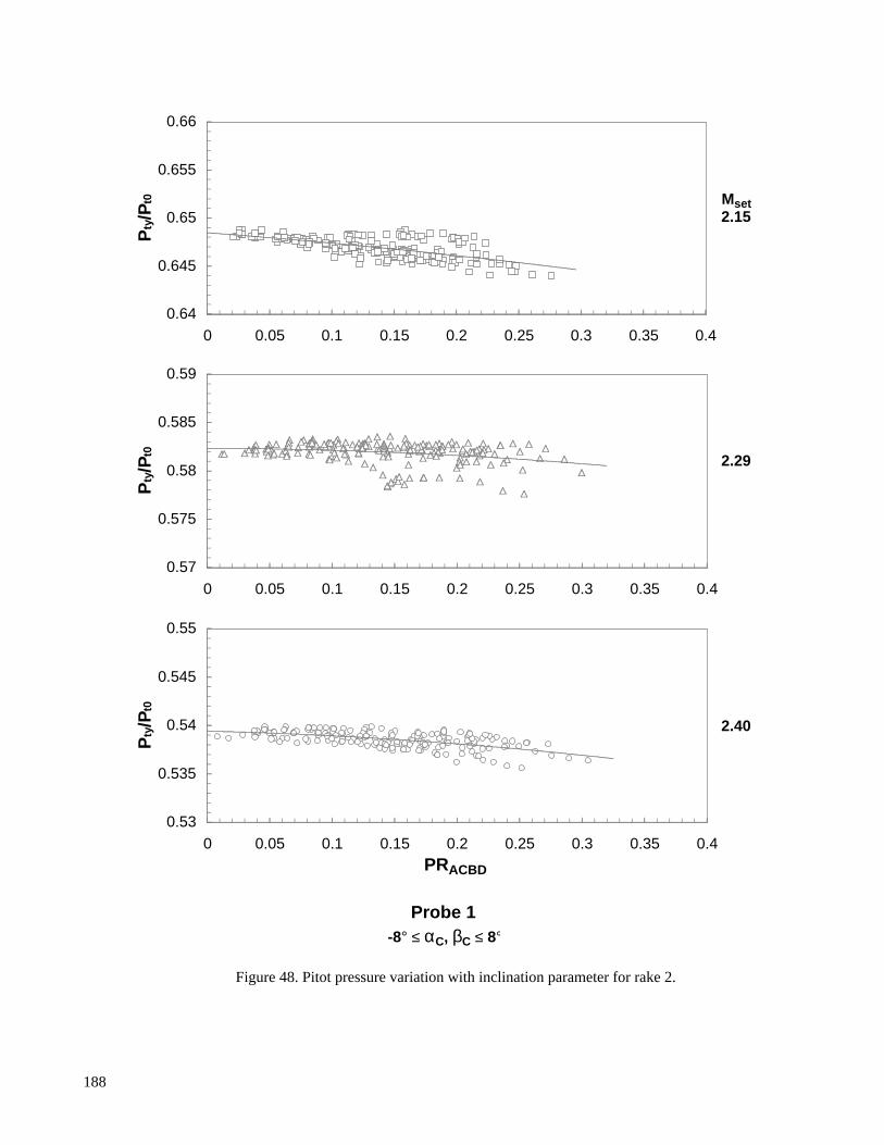
Figure 48. Pitot pressure variation with inclination parameter for rake 2.

0.64

0.645

0.65

0.655

0.66

0 0.05 0.1 0.15 0.2 0.25 0.3 0.35 0.4

Pty/P

t0

0.57

0.575

0.58

0.585

0.59

0 0.05 0.1 0.15 0.2 0.25 0.3 0.35 0.4

Pty/P

t0

0.53

0.535

0.54

0.545

0.55

0 0.05 0.1 0.15 0.2 0.25 0.3 0.35 0.4PRACBD

Pty/P

t0

Probe 1-8° ≤ αC, βC ≤ 8°

Mset2.15

2.29

2.40

188

Figure 48. Continued.

0.635

0.64

0.645

0.65

0.655

0 0.05 0.1 0.15 0.2 0.25 0.3 0.35 0.4

Pty/P

t0

0.57

0.575

0.58

0.585

0.59

0 0.05 0.1 0.15 0.2 0.25 0.3 0.35 0.4

Pty/P

t0

0.53

0.535

0.54

0.545

0.55

0 0.05 0.1 0.15 0.2 0.25 0.3 0.35 0.4PRACBD

Pty/P

t0

Probe 2-8° ≤ αC, βC ≤ 8°

Mset2.15

2.29

2.40

189

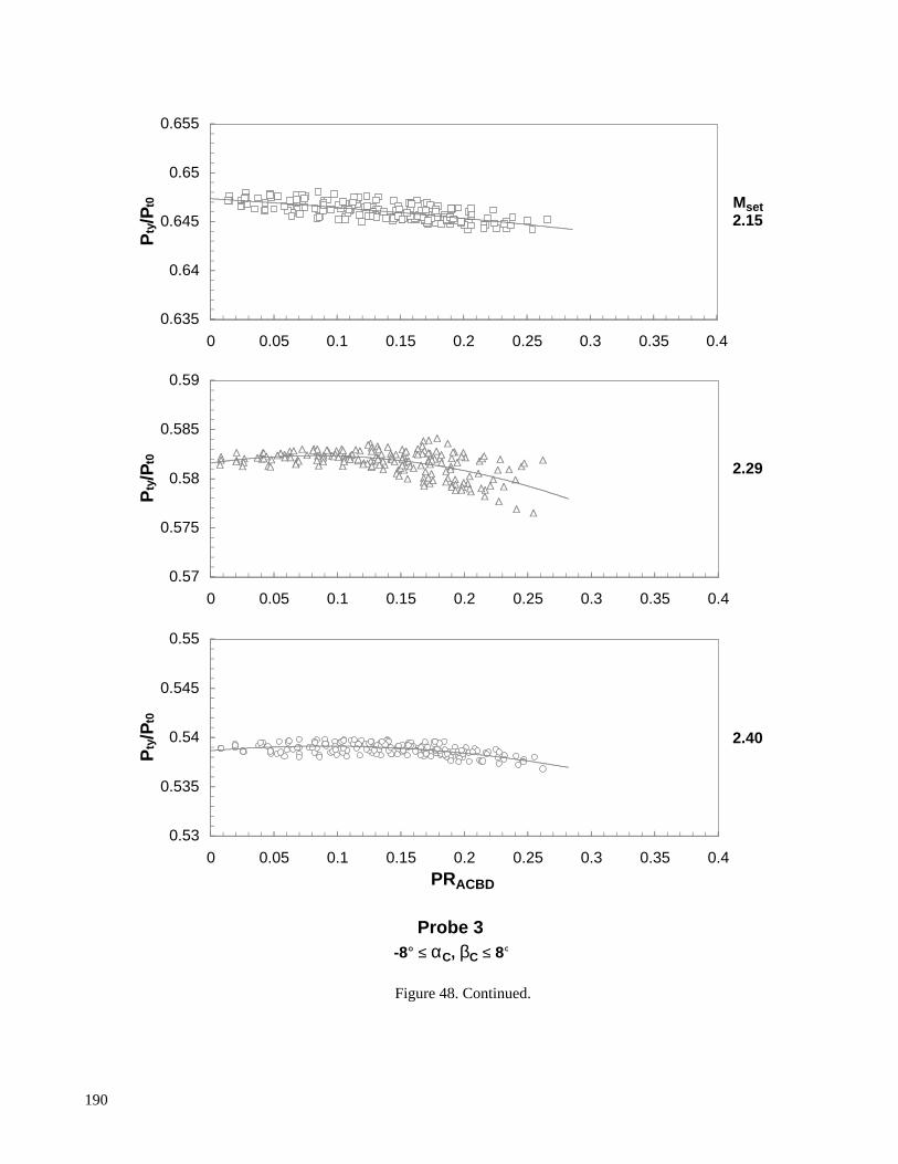
Figure 48. Continued.

0.635

0.64

0.645

0.65

0.655

0 0.05 0.1 0.15 0.2 0.25 0.3 0.35 0.4

Pty/P

t0

0.57

0.575

0.58

0.585

0.59

0 0.05 0.1 0.15 0.2 0.25 0.3 0.35 0.4

Pty/P

t0

0.53

0.535

0.54

0.545

0.55

0 0.05 0.1 0.15 0.2 0.25 0.3 0.35 0.4PRACBD

Pty/P

t0

Probe 3-8° ≤ αC, βC ≤ 8°

Mset2.15

2.29

2.40

190

Figure 48. Continued.

0.635

0.64

0.645

0.65

0.655

0 0.05 0.1 0.15 0.2 0.25 0.3 0.35 0.4

Pty/P

t0

0.57

0.575

0.58

0.585

0.59

0 0.05 0.1 0.15 0.2 0.25 0.3 0.35 0.4

Pty/P

t0

0.53

0.535

0.54

0.545

0.55

0 0.05 0.1 0.15 0.2 0.25 0.3 0.35 0.4PRACBD

Pty/P

t0

Probe 4-8° ≤ αC, βC ≤ 8°

Mset2.15

2.29

2.40

191

Figure 48. Continued.

0.635

0.64

0.645

0.65

0.655

0 0.05 0.1 0.15 0.2 0.25 0.3 0.35 0.4

Pty/P

t0

0.565

0.57

0.575

0.58

0.585

0 0.05 0.1 0.15 0.2 0.25 0.3 0.35 0.4

Pty/P

t0

0.525

0.53

0.535

0.54

0.545

0 0.05 0.1 0.15 0.2 0.25 0.3 0.35 0.4PRACBD

Pty/P

t0

Probe 5-8° ≤ αC, βC ≤ 8°

Mset2.15

2.29

2.40

192

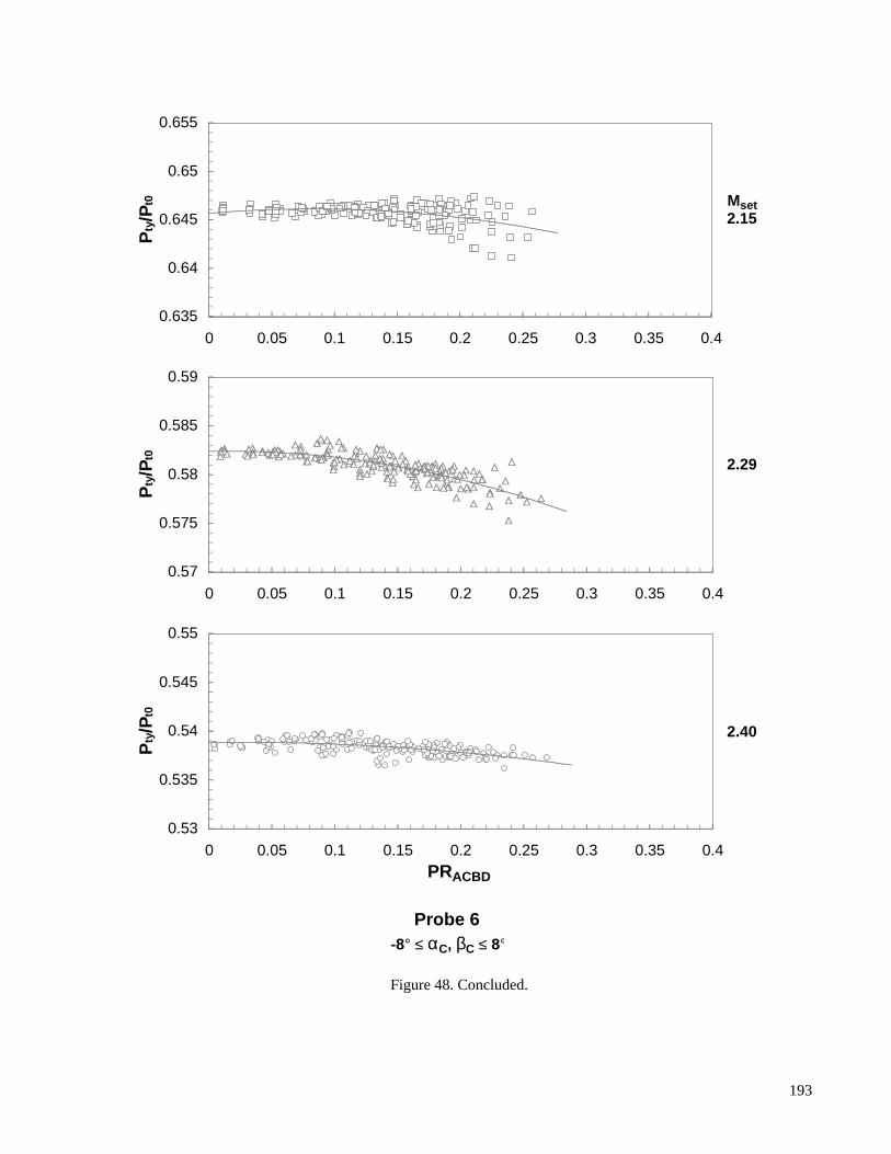
Figure 48. Concluded.

0.635

0.64

0.645

0.65

0.655

0 0.05 0.1 0.15 0.2 0.25 0.3 0.35 0.4

Pty/P

t0

0.57

0.575

0.58

0.585

0.59

0 0.05 0.1 0.15 0.2 0.25 0.3 0.35 0.4

Pty/P

t0

0.53

0.535

0.54

0.545

0.55

0 0.05 0.1 0.15 0.2 0.25 0.3 0.35 0.4PRACBD

Pty/P

t0

Probe 6-8° ≤ αC, βC ≤ 8°

Mset2.15

2.29

2.40

193

194

Figure 49. Cone-probe pitot pressure model.

Figure 50. Converged solution of pitot pressure deviation for rake 1.

0.635

0.64

0.645

0.65

0.655

0 0.1 0.2 0.3 0.4 0.5

Pty/P

t0

0.565

0.57

0.575

0.58

0.585

0 0.1 0.2 0.3 0.4 0.5

Pty/P

t0

0.525

0.53

0.535

0.54

0.545

0 0.1 0.2 0.3 0.4 0.5PRACBDcorrY

Pty/P

t0

Probe 1-8° ≤ αC, βC ≤ 8°

Mset2.15

2.29

2.40

195

Figure 50. Continued.

0.64

0.645

0.65

0.655

0.66

0 0.1 0.2 0.3 0.4 0.5

Pty/P

t0

0.57

0.575

0.58

0.585

0.59

0 0.1 0.2 0.3 0.4 0.5

Pty/P

t0

0.53

0.535

0.54

0.545

0.55

0 0.1 0.2 0.3 0.4 0.5PRACBDcorrY

Pty/P

t0

Probe 2-8° ≤ αC, βC ≤ 8°

Mset2.15

2.29

2.40

196

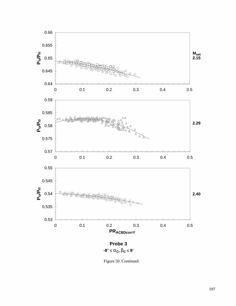
Figure 50. Continued.

0.64

0.645

0.65

0.655

0.66

0 0.1 0.2 0.3 0.4 0.5

Pty/P

t0

0.57

0.575

0.58

0.585

0.59

0 0.1 0.2 0.3 0.4 0.5

Pty/P

t0

0.53

0.535

0.54

0.545

0.55

0 0.1 0.2 0.3 0.4 0.5PRACBDcorrY

Pty/P

t0

Probe 3-8° ≤ αC, βC ≤ 8°

Mset2.15

2.29

2.40

197

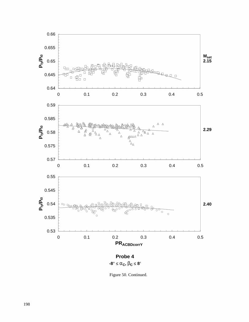
Figure 50. Continued.

0.64

0.645

0.65

0.655

0.66

0 0.1 0.2 0.3 0.4 0.5

Pty/P

t0

0.57

0.575

0.58

0.585

0.59

0 0.1 0.2 0.3 0.4 0.5

Pty/P

t0

0.53

0.535

0.54

0.545

0.55

0 0.1 0.2 0.3 0.4 0.5PRACBDcorrY

Pty/P

t0

Probe 4-8° ≤ αC, βC ≤ 8°

Mset2.15

2.29

2.40

198

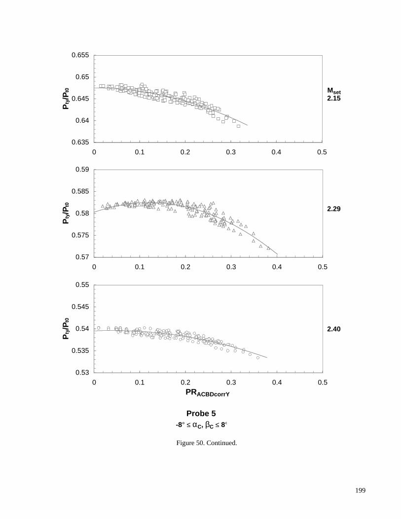
Figure 50. Continued.

0.635

0.64

0.645

0.65

0.655

0 0.1 0.2 0.3 0.4 0.5

Pty/P

t0

0.57

0.575

0.58

0.585

0.59

0 0.1 0.2 0.3 0.4 0.5

Pty/P

t0

0.53

0.535

0.54

0.545

0.55

0 0.1 0.2 0.3 0.4 0.5PRACBDcorrY

Pty/P

t0

Probe 5-8° ≤ αC, βC ≤ 8°

Mset2.15

2.29

2.40

199

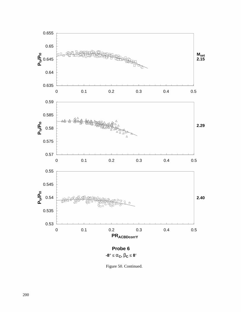
Figure 50. Continued.

0.635

0.64

0.645

0.65

0.655

0 0.1 0.2 0.3 0.4 0.5

Pty/P

t0

0.57

0.575

0.58

0.585

0.59

0 0.1 0.2 0.3 0.4 0.5

Pty/P

t0

0.53

0.535

0.54

0.545

0.55

0 0.1 0.2 0.3 0.4 0.5PRACBDcorrY

Pty/P

t0

Probe 6-8° ≤ αC, βC ≤ 8°

Mset2.15

2.29

2.40

200

Figure 50. Continued.

0.635

0.64

0.645

0.65

0.655

0 0.1 0.2 0.3 0.4 0.5

Pty/P

t0

0.57

0.575

0.58

0.585

0.59

0 0.1 0.2 0.3 0.4 0.5

Pty/P

t0

0.53

0.535

0.54

0.545

0.55

0.3 0.4 0.5 0.6 0.7 0.8PRACBDcorrY

Pty/P

t0

Probe 7-8° ≤ αC, βC ≤ 8°

Mset2.15

2.29

2.40

201

Figure 50. Concluded.

0.63

0.635

0.64

0.645

0.65

0 0.1 0.2 0.3 0.4 0.5

Pty/P

t0

0.565

0.57

0.575

0.58

0.585

0 0.1 0.2 0.3 0.4 0.5

Pty/P

t0

0.525

0.53

0.535

0.54

0.545

0 0.1 0.2 0.3 0.4 0.5PRACBDcorrY

Pty/P

t0

Probe 8-8° ≤ αC, βC ≤ 8°

Mset2.15

2.29

2.40

202

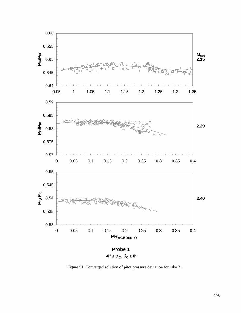
Figure 51. Converged solution of pitot pressure deviation for rake 2.

0.64

0.645

0.65

0.655

0.66

0.95 1 1.05 1.1 1.15 1.2 1.25 1.3 1.35

Pty/P

t0

0.57

0.575

0.58

0.585

0.59

0 0.05 0.1 0.15 0.2 0.25 0.3 0.35 0.4

Pty/P

t0

0.53

0.535

0.54

0.545

0.55

0 0.05 0.1 0.15 0.2 0.25 0.3 0.35 0.4PRACBDcorrY

Pty/P

t0

Probe 1-8° ≤ αC, βC ≤ 8°

Mset2.15

2.29

2.40

203

Figure 51. Continued.

0.635

0.64

0.645

0.65

0.655

0 0.05 0.1 0.15 0.2 0.25 0.3 0.35 0.4

Pty/P

t0

0.57

0.575

0.58

0.585

0.59

0 0.05 0.1 0.15 0.2 0.25 0.3 0.35 0.4

Pty/P

t0

0.53

0.535

0.54

0.545

0.55

0 0.05 0.1 0.15 0.2 0.25 0.3 0.35 0.4PRACBDcorrY

Pty/P

t0

Probe 2-8° ≤ αC, βC ≤ 8°

Mset2.15

2.29

2.40

204

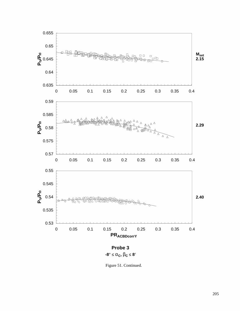
Figure 51. Continued.

0.635

0.64

0.645

0.65

0.655

0 0.05 0.1 0.15 0.2 0.25 0.3 0.35 0.4

Pty/P

t0

0.57

0.575

0.58

0.585

0.59

0 0.05 0.1 0.15 0.2 0.25 0.3 0.35 0.4

Pty/P

t0

0.53

0.535

0.54

0.545

0.55

0 0.05 0.1 0.15 0.2 0.25 0.3 0.35 0.4PRACBDcorrY

Pty/P

t0

Probe 3-8° ≤ αC, βC ≤ 8°

Mset2.15

2.29

2.40

205

Figure 51. Continued.

0.635

0.64

0.645

0.65

0.655

0 0.05 0.1 0.15 0.2 0.25 0.3 0.35 0.4

Pty/P

t0

0.57

0.575

0.58

0.585

0.59

0 0.05 0.1 0.15 0.2 0.25 0.3 0.35 0.4

Pty/P

t0

0.53

0.535

0.54

0.545

0.55

0 0.05 0.1 0.15 0.2 0.25 0.3 0.35 0.4PRACBDcorrY

Pty/P

t0

Probe 4-8° ≤ αC, βC ≤ 8°

Mset2.15

2.29

2.40

206

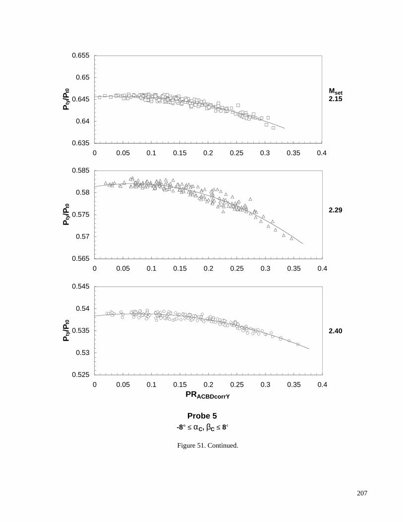
Figure 51. Continued.

0.635

0.64

0.645

0.65

0.655

0 0.05 0.1 0.15 0.2 0.25 0.3 0.35 0.4

Pty/P

t0

0.565

0.57

0.575

0.58

0.585

0 0.05 0.1 0.15 0.2 0.25 0.3 0.35 0.4

Pty/P

t0

0.525

0.53

0.535

0.54

0.545

0 0.05 0.1 0.15 0.2 0.25 0.3 0.35 0.4PRACBDcorrY

Pty/P

t0

Probe 5-8° ≤ αC, βC ≤ 8°

Mset2.15

2.29

2.40

207

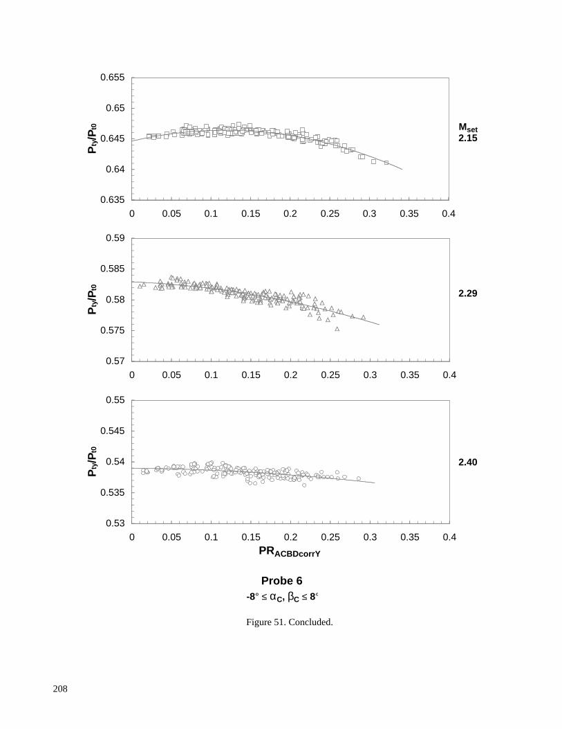
Figure 51. Concluded.

0.635

0.64

0.645

0.65

0.655

0 0.05 0.1 0.15 0.2 0.25 0.3 0.35 0.4

Pty/P

t0

0.57

0.575

0.58

0.585

0.59

0 0.05 0.1 0.15 0.2 0.25 0.3 0.35 0.4

Pty/P

t0

0.53

0.535

0.54

0.545

0.55

0 0.05 0.1 0.15 0.2 0.25 0.3 0.35 0.4PRACBDcorrY

Pty/P

t0

Probe 6-8° ≤ αC, βC ≤ 8°

Mset2.15

2.29

2.40

208

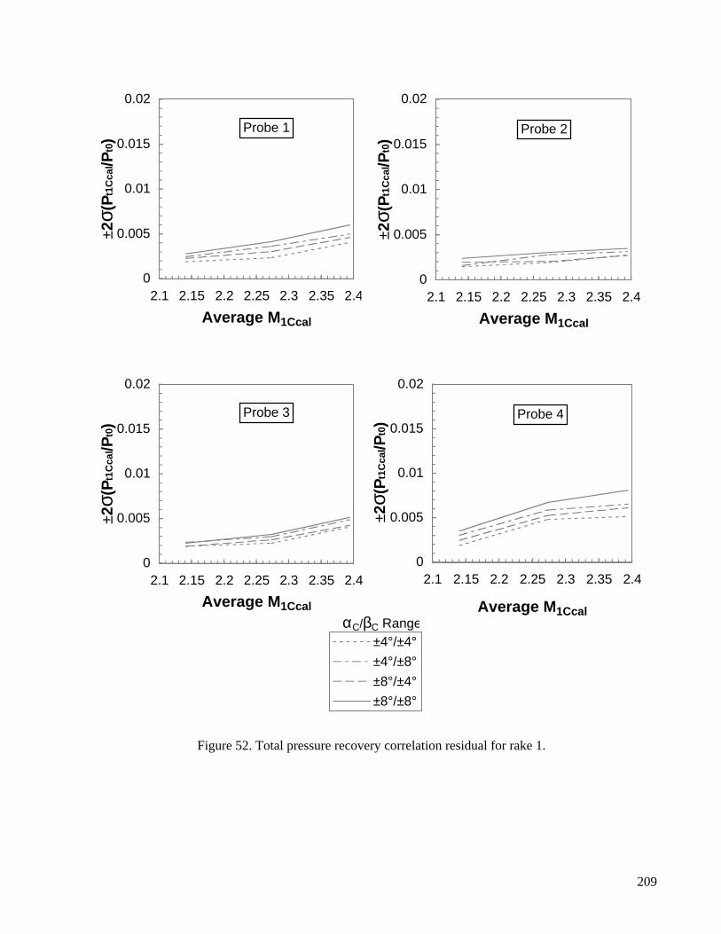
Figure 52. Total pressure recovery correlation residual for rake 1.

0

0.005

0.01

0.015

0.02

2.1 2.15 2.2 2.25 2.3 2.35 2.4

Average M1Ccal

±2σ(

Pt1

Cca

l/Pt0)

Probe 1

0

0.005

0.01

0.015

0.02

2.1 2.15 2.2 2.25 2.3 2.35 2.4

Average M1Ccal

±2σ(

Pt1

Cca

l/Pt0)

Probe 2

0

0.005

0.01

0.015

0.02

2.1 2.15 2.2 2.25 2.3 2.35 2.4

Average M1Ccal

±2σ(

Pt1

Cca

l/Pt0)

Probe 3

0

0.005

0.01

0.015

0.02

2.1 2.15 2.2 2.25 2.3 2.35 2.4

Average M1Ccal

±2σ(

Pt1

Cca

l/Pt0)

±4°/±4°±4°/±8°±8°/±4°±8°/±8°

Probe 4

αC/βC Range

209

Figure 52. Concluded.

0

0.005

0.01

0.015

0.02

2.1 2.15 2.2 2.25 2.3 2.35 2.4

Average M1Ccal

±2σ(

Pt1

Cca

l/Pt0)

Probe 5

0

0.005

0.01

0.015

0.02

2.1 2.15 2.2 2.25 2.3 2.35 2.4

Average M1Ccal

±2σ(

Pt1

Cca

l/Pt0)

Probe 6

0

0.005

0.01

0.015

0.02

2.1 2.15 2.2 2.25 2.3 2.35 2.4

Average M1Ccal

±2σ(

Pt1

Cca

l/Pt0)

Probe 7

0

0.005

0.01

0.015

0.02

2.1 2.15 2.2 2.25 2.3 2.35 2.4

Average M1Ccal

±2σ(

Pt1

Cca

l/Pt0)

±4°/±4°±4°/±8°±8°/±4°±8°/±8°

Probe 8

αC/βC Range

210

Figure 53. Total pressure recovery correlation residual for rake 2.

0

0.005

0.01

0.015

0.02

2.1 2.15 2.2 2.25 2.3 2.35 2.4

Average M1Ccal

±2σ(

Pt1

Cca

l/Pt0)

Probe 1

0

0.005

0.01

0.015

0.02

2.1 2.15 2.2 2.25 2.3 2.35 2.4

Average M1Ccal

±2σ(

Pt1

Cca

l/Pt0)

Probe 2

0

0.005

0.01

0.015

0.02

2.1 2.15 2.2 2.25 2.3 2.35 2.4

Average M1Ccal

±2σ(

Pt1

Cca

l/Pt0)

Probe 3

0

0.005

0.01

0.015

0.02

2.1 2.15 2.2 2.25 2.3 2.35 2.4

Average M1Ccal

±2σ(

Pt1

Cca

l/Pt0)

±4°/±4°±4°/±8°±8°/±4°±8°/±8°

Probe 4

αC/βC Range

211

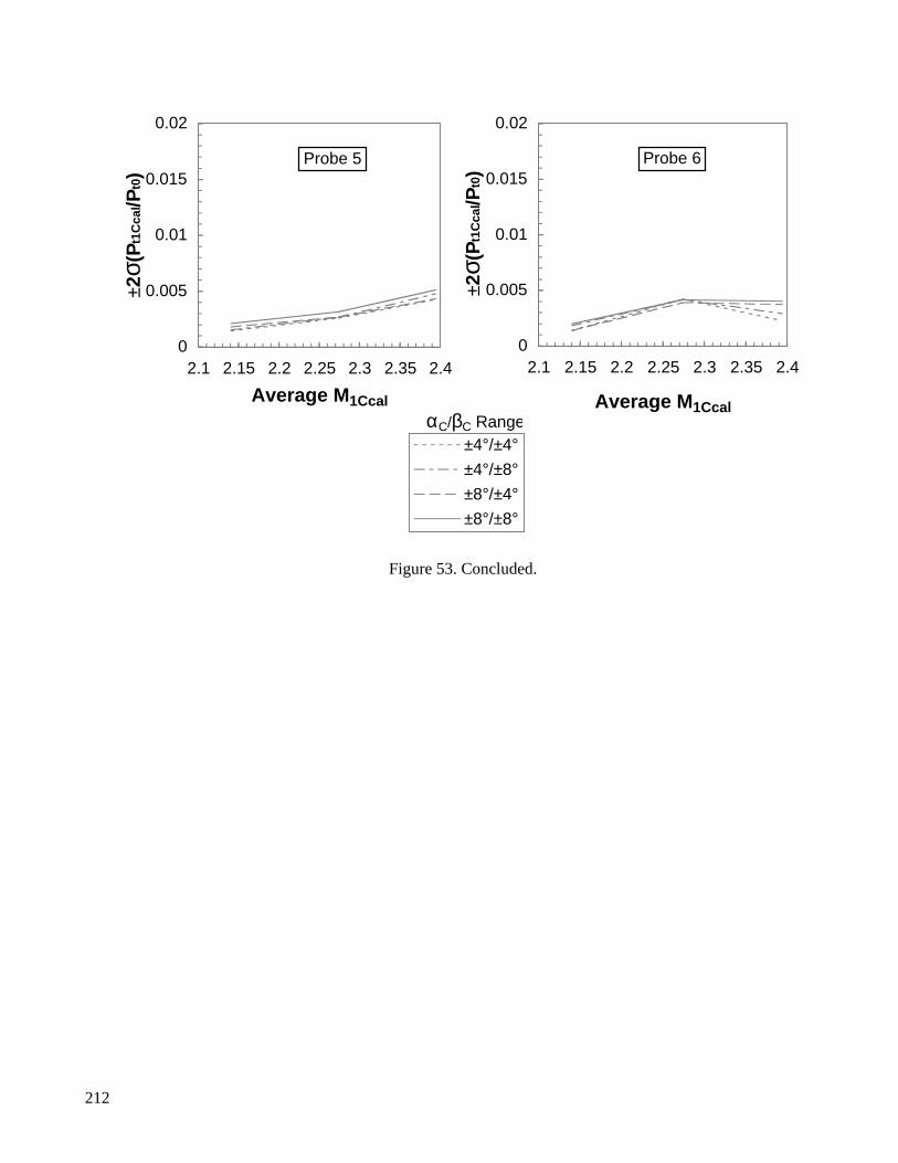
Figure 53. Concluded.

0

0.005

0.01

0.015

0.02

2.1 2.15 2.2 2.25 2.3 2.35 2.4

Average M1Ccal

±2σ(

Pt1

Cca

l/Pt0)

Probe 5

0

0.005

0.01

0.015

0.02

2.1 2.15 2.2 2.25 2.3 2.35 2.4

Average M1Ccal

±2σ(

Pt1

Cca

l/Pt0)

±4°/±4°±4°/±8°±8°/±4°±8°/±8°

Probe 6

αC/βC Range

212

Figure 54. Cone-probe angle of attack variation for rake 1 at Mset = 2.40.

-15

-10

-5

0

5

10

15

-0.3 -0.2 -0.1 0 0.1 0.2 0.3

PRAC

αC (d

eg)

Probe 1Mset = 2.40, Nominal βC = 0°

213

Figure 54. Continued.

-15

-10

-5

0

5

10

15

-0.3 -0.2 -0.1 0 0.1 0.2 0.3PRAC

αC (d

eg)

Probe 2Mset = 2.40, Nominal βC = 0°

214

Figure 54. Continued.

-15

-10

-5

0

5

10

15

-0.3 -0.2 -0.1 0 0.1 0.2 0.3PRAC

αC (d

eg)

Probe 3Mset = 2.40, Nominal βC = 0°

215

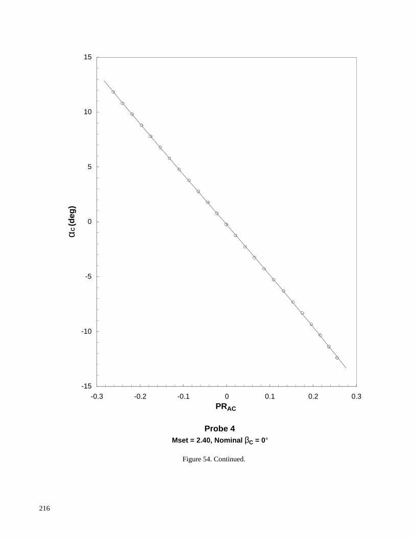
Figure 54. Continued.

-15

-10

-5

0

5

10

15

-0.3 -0.2 -0.1 0 0.1 0.2 0.3PRAC

αC (d

eg)

Probe 4Mset = 2.40, Nominal βC = 0°

216

Figure 54. Continued.

-15

-10

-5

0

5

10

15

-0.3 -0.2 -0.1 0 0.1 0.2 0.3PRAC

αC (d

eg)

Probe 5Mset = 2.40, Nominal βC = 0°

217

Figure 54. Continued.

-15

-10

-5

0

5

10

15

-0.3 -0.2 -0.1 0 0.1 0.2 0.3PRAC

αC (d

eg)

Probe 6Mset = 2.40, Nominal βC = 0°

218

Figure 54. Continued.

-15

-10

-5

0

5

10

15

-0.3 -0.2 -0.1 0 0.1 0.2 0.3PRAC

αC (d

eg)

Probe 7Mset = 2.40, Nominal βC = 0°

219

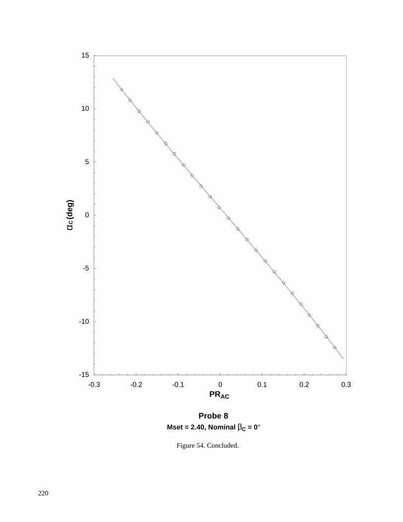
Figure 54. Concluded.

-15

-10

-5

0

5

10

15

-0.3 -0.2 -0.1 0 0.1 0.2 0.3PRAC

αC (d

eg)

Probe 8Mset = 2.40, Nominal βC = 0°

220

Figure 55. Cone-probe angle of attack variation for rake 2 at Mset =2.40.

-15

-10

-5

0

5

10

15

-0.3 -0.2 -0.1 0 0.1 0.2 0.3

PRAC

αC (d

eg)

Probe 1Mset = 2.40, Nominal βC = 0°

221

Figure 55. Continued.

-15

-10

-5

0

5

10

15

-0.3 -0.2 -0.1 0 0.1 0.2 0.3PRAC

αC (d

eg)

Probe 2Mset = 2.40, Nominal βC = 0°

222

Figure 55. Continued.

-15

-10

-5

0

5

10

15

-0.3 -0.2 -0.1 0 0.1 0.2 0.3PRAC

αC (d

eg)

Probe 3Mset = 2.40, Nominal βC = 0°

223

Figure 55. Continued.

-15

-10

-5

0

5

10

15

-0.3 -0.2 -0.1 0 0.1 0.2 0.3PRAC

αC (d

eg)

Probe 4Mset = 2.40, Nominal βC = 0°

224

Figure 55. Continued.

-15

-10

-5

0

5

10

15

-0.3 -0.2 -0.1 0 0.1 0.2 0.3PRAC

αC (d

eg)

Probe 5Mset = 2.40, Nominal βC = 0°

225

Figure 55. Concluded.

-15

-10

-5

0

5

10

15

-0.3 -0.2 -0.1 0 0.1 0.2 0.3PRAC

αC (d

eg)

Probe 6Mset = 2.40, Nominal βC = 0°

226

Figure 56. Angle of attack correlation residual for rake 1.

0

0.05

0.1

0.15

0.2

2.1 2.15 2.2 2.25 2.3 2.35 2.4

Average M1Ccal

±2σ(

αCca

l), d

egProbe 1

0

0.05

0.1

0.15

0.2

2.1 2.15 2.2 2.25 2.3 2.35 2.4

Average M1Ccal

±2σ(

αCca

l), d

eg

Probe 2

0

0.05

0.1

0.15

0.2

2.1 2.15 2.2 2.25 2.3 2.35 2.4

Average M1Ccal

±2σ(

αCca

l), d

eg

Probe 3

0

0.05

0.1

0.15

0.2

2.1 2.15 2.2 2.25 2.3 2.35 2.4

Average M1Ccal

±2σ(

αCca

l), d

eg

±4°/±4°±4°/±8°±8°/±4°±8°/±8°

Probe 4

αC/βC Range

227

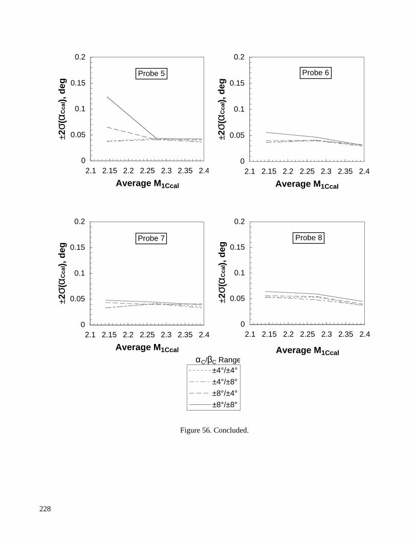
Figure 56. Concluded.

0

0.05

0.1

0.15

0.2

2.1 2.15 2.2 2.25 2.3 2.35 2.4

Average M1Ccal

±2σ(

αCca

l), d

egProbe 5

0

0.05

0.1

0.15

0.2

2.1 2.15 2.2 2.25 2.3 2.35 2.4

Average M1Ccal

±2σ(

αCca

l), d

eg

Probe 6

0

0.05

0.1

0.15

0.2

2.1 2.15 2.2 2.25 2.3 2.35 2.4

Average M1Ccal

±2σ(

αCca

l), d

eg

Probe 7

0

0.05

0.1

0.15

0.2

2.1 2.15 2.2 2.25 2.3 2.35 2.4

Average M1Ccal

±2σ(

αCca

l), d

eg

±4°/±4°±4°/±8°±8°/±4°±8°/±8°

Probe 8

αC/βC Range

228

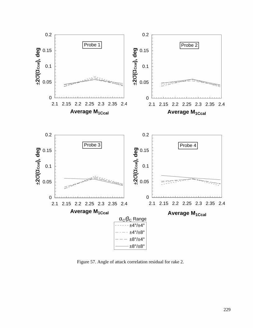
Figure 57. Angle of attack correlation residual for rake 2.

0

0.05

0.1

0.15

0.2

2.1 2.15 2.2 2.25 2.3 2.35 2.4

Average M1Ccal

±2σ(

αCca

l), d

egProbe 1

0

0.05

0.1

0.15

0.2

2.1 2.15 2.2 2.25 2.3 2.35 2.4

Average M1Ccal

±2σ(

αCca

l), d

eg

Probe 2

0

0.05

0.1

0.15

0.2

2.1 2.15 2.2 2.25 2.3 2.35 2.4

Average M1Ccal

±2σ(

αCca

l), d

eg

Probe 3

0

0.05

0.1

0.15

0.2

2.1 2.15 2.2 2.25 2.3 2.35 2.4

Average M1Ccal

±2σ(

αCca

l), d

eg

±4°/±4°±4°/±8°±8°/±4°±8°/±8°

Probe 4

αC/βC Range

229

Figure 57. Concluded.

0

0.05

0.1

0.15

0.2

2.1 2.15 2.2 2.25 2.3 2.35 2.4

Average M1Ccal

±2σ(

αCca

l), d

egProbe 5

0

0.05

0.1

0.15

0.2

2.1 2.15 2.2 2.25 2.3 2.35 2.4

Average M1Ccal

±2σ(

αCca

l), d

eg

±4°/±4°±4°/±8°±8°/±4°±8°/±8°

Probe 6

αC/βC Range

230

Figure 58. Cone-probe angle of sideslip variation for rake 1 at Mset = 2.40.

-10

-8

-6

-4

-2

0

2

4

6

8

10

-0.2 -0.15 -0.1 -0.05 0 0.05 0.1 0.15 0.2

PRBD

βC (d

eg)

Probe 1Mset = 2.40, Nominal αC = 0°

231

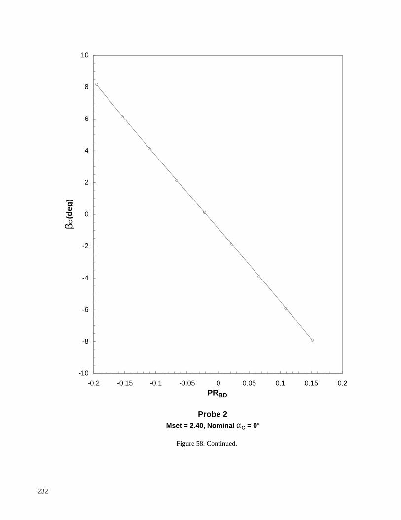
Figure 58. Continued.

-10

-8

-6

-4

-2

0

2

4

6

8

10

-0.2 -0.15 -0.1 -0.05 0 0.05 0.1 0.15 0.2PRBD

βC (d

eg)

Probe 2Mset = 2.40, Nominal αC = 0°

232

Figure 58. Continued.

-10

-8

-6

-4

-2

0

2

4

6

8

10

-0.25 -0.2 -0.15 -0.1 -0.05 0 0.05 0.1 0.15PRBD

βC (d

eg)

Probe 3Mset = 2.40, Nominal αC = 0°

233

Figure 58. Continued.

-10

-8

-6

-4

-2

0

2

4

6

8

10

-0.2 -0.15 -0.1 -0.05 0 0.05 0.1 0.15 0.2PRBD

βC (d

eg)

Probe 4Mset = 2.40, Nominal αC = 0°

234

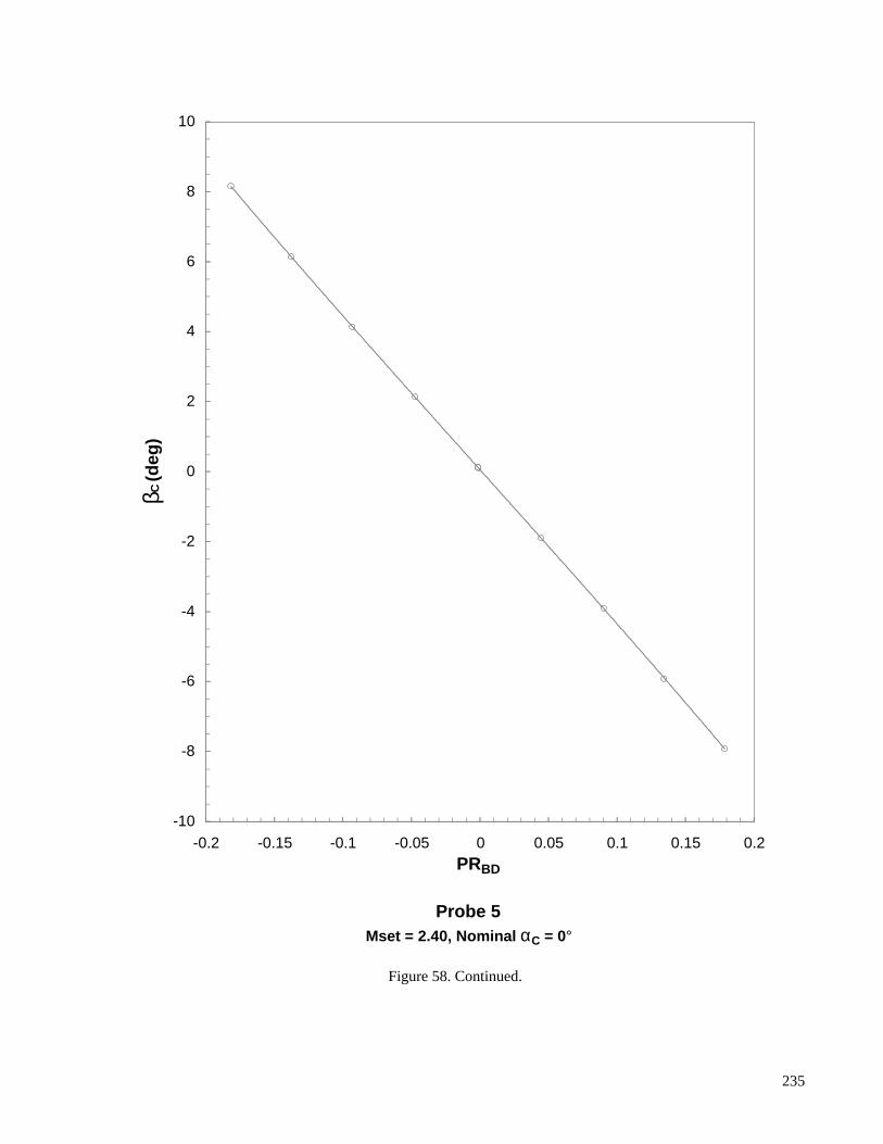
Figure 58. Continued.

-10

-8

-6

-4

-2

0

2

4

6

8

10

-0.2 -0.15 -0.1 -0.05 0 0.05 0.1 0.15 0.2PRBD

βC (d

eg)

Probe 5Mset = 2.40, Nominal αC = 0°

235

Figure 58. Continued.

-10

-8

-6

-4

-2

0

2

4

6

8

10

-0.2 -0.15 -0.1 -0.05 0 0.05 0.1 0.15 0.2PRBD

βC (d

eg)

Probe 6Mset = 2.40, Nominal αC = 0°

236

Figure 58. Continued.

-10

-8

-6

-4

-2

0

2

4

6

8

10

-0.2 -0.15 -0.1 -0.05 0 0.05 0.1 0.15 0.2PRBD

βC (d

eg)

Probe 7Mset = 2.40, Nominal αC = 0°

237

Figure 58. Concluded.

-10

-8

-6

-4

-2

0

2

4

6

8

10

-0.2 -0.15 -0.1 -0.05 0 0.05 0.1 0.15 0.2PRBD

βC (d

eg)

Probe 8Mset = 2.40, Nominal αC = 0°

238

Figure 59. Cone-probe angle of sideslip variation for rake 2 at Mset = 2.40.

-10

-8

-6

-4

-2

0

2

4

6

8

10

-0.25 -0.2 -0.15 -0.1 -0.05 0 0.05 0.1 0.15

PRBD

βC (d

eg)

Probe 1Mset = 2.40, Nominal αC = 0°

239

Figure 59. Continued.

-10

-8

-6

-4

-2

0

2

4

6

8

10

-0.2 -0.15 -0.1 -0.05 0 0.05 0.1 0.15 0.2PRBD

βC (d

eg)

Probe 2Mset = 2.40, Nominal αC = 0°

240

Figure 59. Continued.

-10

-8

-6

-4

-2

0

2

4

6

8

10

-0.2 -0.15 -0.1 -0.05 0 0.05 0.1 0.15 0.2PRBD

βC (d

eg)

Probe 3Mset = 2.40, Nominal αC = 0°

241

Figure 59. Continued.

-10

-8

-6

-4

-2

0

2

4

6

8

10

-0.25 -0.2 -0.15 -0.1 -0.05 0 0.05 0.1 0.15PRBD

βC (d

eg)

Probe 4Mset = 2.40, Nominal αC = 0°

242

Figure 59. Continued.

-10

-8

-6

-4

-2

0

2

4

6

8

10

-0.25 -0.2 -0.15 -0.1 -0.05 0 0.05 0.1 0.15PRBD

βC (d

eg)

Probe 5Mset = 2.40, Nominal αC = 0°

243

Figure 59. Concluded.

-10

-8

-6

-4

-2

0

2

4

6

8

10

-0.2 -0.15 -0.1 -0.05 0 0.05 0.1 0.15 0.2PRBD

βC (d

eg)

Probe 6Mset = 2.40, Nominal αC = 0°

244

Figure 60. Angle of sideslip correlation residual for rake 1.

0

0.05

0.1

0.15

0.2

2.1 2.15 2.2 2.25 2.3 2.35 2.4

Average M1Ccal

±2σ(

βCca

l), d

egProbe 1

0

0.05

0.1

0.15

0.2

2.1 2.15 2.2 2.25 2.3 2.35 2.4

Average M1Ccal

±2σ(

βCca

l), d

eg

Probe 2

0

0.05

0.1

0.15

0.2

2.1 2.15 2.2 2.25 2.3 2.35 2.4

Average M1Ccal

±2σ(

βCca

l), d

eg

Probe 3

0

0.05

0.1

0.15

0.2

2.1 2.15 2.2 2.25 2.3 2.35 2.4

Average M1Ccal

±2σ(

βCca

l), d

eg

±4°/±4°±4°/±8°±8°/±4°±8°/±8°

Probe 4

αC/βC Range

245

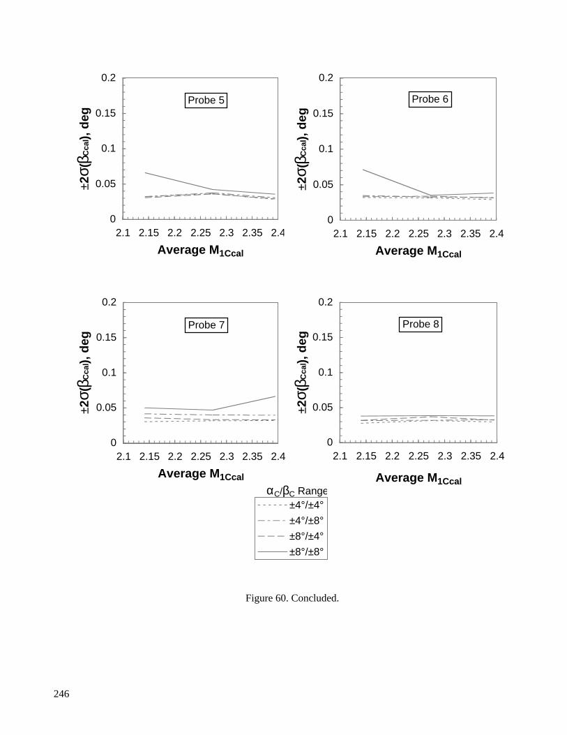
Figure 60. Concluded.

0

0.05

0.1

0.15

0.2

2.1 2.15 2.2 2.25 2.3 2.35 2.4

Average M1Ccal

±2σ(

βCca

l), d

egProbe 5

0

0.05

0.1

0.15

0.2

2.1 2.15 2.2 2.25 2.3 2.35 2.4

Average M1Ccal

±2σ(

βCca

l), d

eg

Probe 6

0

0.05

0.1

0.15

0.2

2.1 2.15 2.2 2.25 2.3 2.35 2.4

Average M1Ccal

±2σ(

βCca

l), d

eg

Probe 7

0

0.05

0.1

0.15

0.2

2.1 2.15 2.2 2.25 2.3 2.35 2.4

Average M1Ccal

±2σ(

βCca

l), d

eg

±4°/±4°±4°/±8°±8°/±4°±8°/±8°

Probe 8

αC/βC Range

246

Figure 61. Angle of sideslip correlation residual for rake 2.

0

0.05

0.1

0.15

0.2

2.1 2.15 2.2 2.25 2.3 2.35 2.4

Average M1Ccal

±2σ(

βCca

l), d

egProbe 1

0

0.05

0.1

0.15

0.2

2.1 2.15 2.2 2.25 2.3 2.35 2.4

Average M1Ccal

±2σ(

βCca

l), d

eg

Probe 2

0

0.05

0.1

0.15

0.2

2.1 2.15 2.2 2.25 2.3 2.35 2.4

Average M1Ccal

±2σ(

βCca

l), d

eg

Probe 3

0

0.05

0.1

0.15

0.2

2.1 2.15 2.2 2.25 2.3 2.35 2.4

Average M1Ccal

±2σ(

βCca

l), d

eg

±4°/±4°±4°/±8°±8°/±4°±8°/±8°

Probe 4

αC/βC Range

247

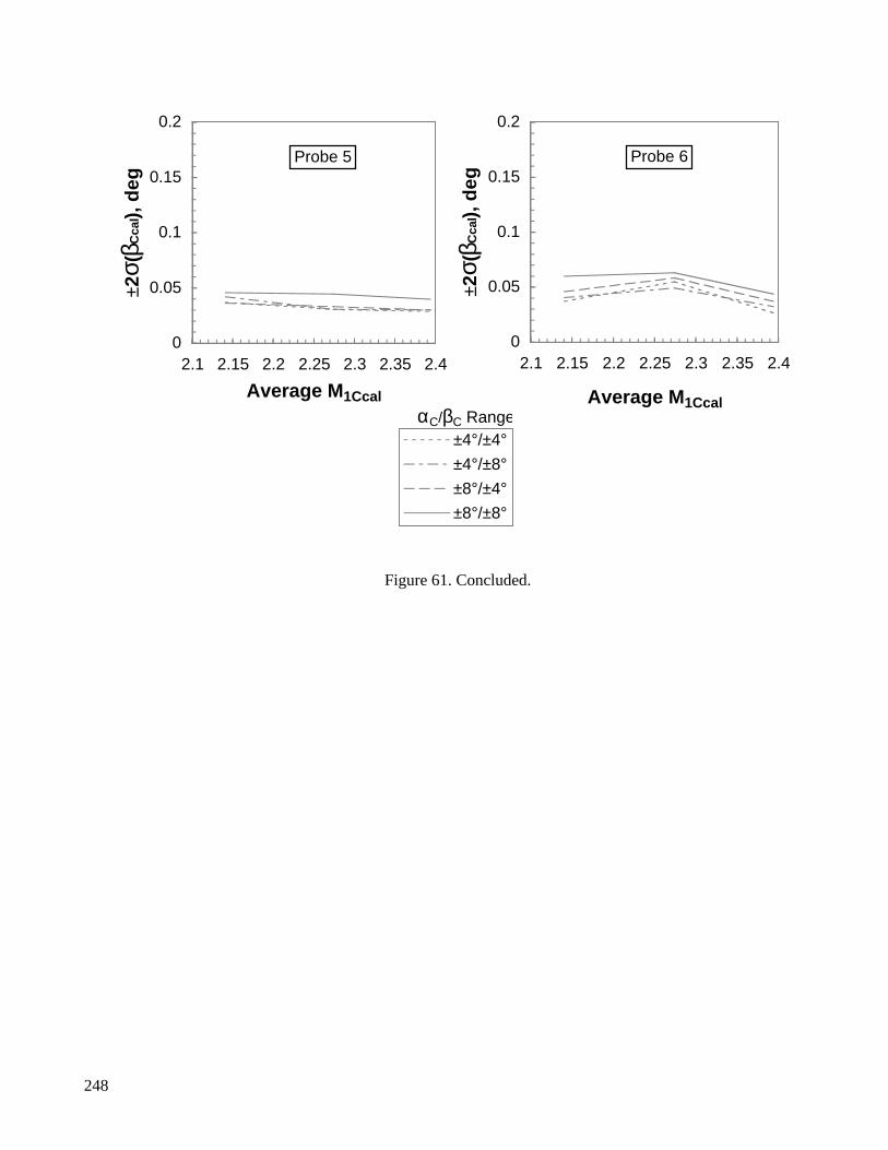
Figure 61. Concluded.

0

0.05

0.1

0.15

0.2

2.1 2.15 2.2 2.25 2.3 2.35 2.4

Average M1Ccal

±2σ(

βCca

l), d

egProbe 5

0

0.05

0.1

0.15

0.2

2.1 2.15 2.2 2.25 2.3 2.35 2.4

Average M1Ccal

±2σ(

βCca

l), d

eg

±4°/±4°±4°/±8°±8°/±4°±8°/±8°

Probe 6

αC/βC Range

248

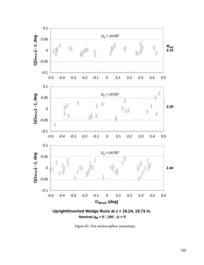
Figure 62. Test section upflow uncertainty.

-0.1

-0.05

0

0.05

0.1

-0.5 -0.4 -0.3 -0.2 -0.1 0 0.1 0.2 0.3 0.4 0.5

ε( αW

corr)

- ε, d

egUµ = ±0.05°

-0.1

-0.05

0

0.05

0.1

-0.5 -0.4 -0.3 -0.2 -0.1 0 0.1 0.2 0.3 0.4 0.5

ε( αW

corr)

- ε, d

eg

Uµ = ±0.05°

-0.1

-0.05

0

0.05

0.1

-0.5 -0.4 -0.3 -0.2 -0.1 0 0.1 0.2 0.3 0.4 0.5

αWcorr (deg)

ε( αW

corr)

- ε, d

eg

Uµ = ±0.05°

Upright/Inverted Wedge Runs at z = 16.24, 19.73 in. Nominal φM = 0°, 180°, ψ = 0°

Mset2.15

2.29

2.40

249

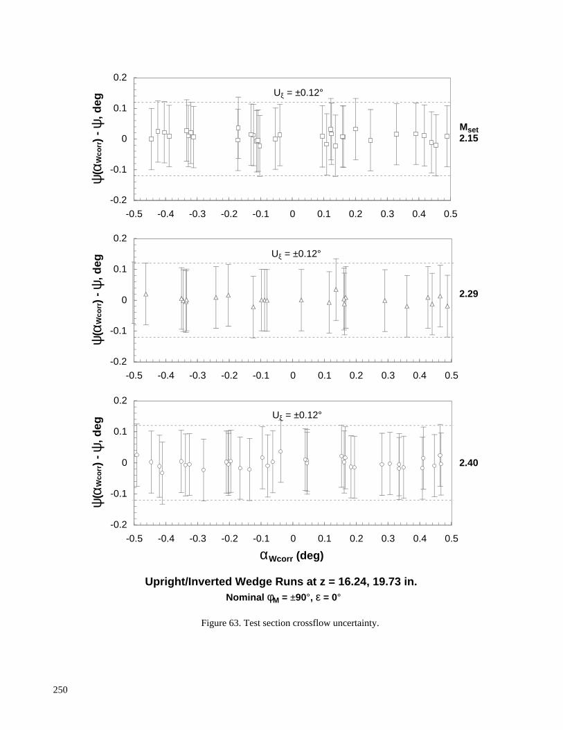
Figure 63. Test section crossflow uncertainty.

-0.2

-0.1

0

0.1

0.2

-0.5 -0.4 -0.3 -0.2 -0.1 0 0.1 0.2 0.3 0.4 0.5

ψ( α

Wco

rr)

- ψ, d

egUξ = ±0.12°

-0.2

-0.1

0

0.1

0.2

-0.5 -0.4 -0.3 -0.2 -0.1 0 0.1 0.2 0.3 0.4 0.5

ψ( α

Wco

rr)

- ψ, d

eg

Uξ = ±0.12°

-0.2

-0.1

0

0.1

0.2

-0.5 -0.4 -0.3 -0.2 -0.1 0 0.1 0.2 0.3 0.4 0.5

αWcorr (deg)

ψ( α

Wco

rr)

- ψ, d

eg

Uξ = ±0.12°

Upright/Inverted Wedge Runs at z = 16.24, 19.73 in. Nominal φM = ±90°, ε = 0°

Mset2.15

2.29

2.40

250

Figure 64. Test section Mach number uncertainty for Method III calculation.

-0.01

-0.005

0

0.005

0.01

2.137 2.138 2.139 2.14 2.141 2.142 2.143 2.144

M1(

z) E

rro

rUM1 = ±0.005

-0.01

-0.005

0

0.005

0.01

2.268 2.27 2.272 2.274 2.276 2.278 2.28 2.282 2.284

M1(

z) E

rro

r

UM1 = ±0.005

-0.01

-0.005

0

0.005

0.01

2.39 2.391 2.392 2.393 2.394 2.395 2.396 2.397 2.398

M1,III

M1(

z) E

rro

r

UM1 = ±0.005

Upright/Inverted Wedge Runs at z = 16.24, 19.73 in. Nominal ε, ψ within ±0.25° of stream angle

Mset2.15

2.29

2.40

251

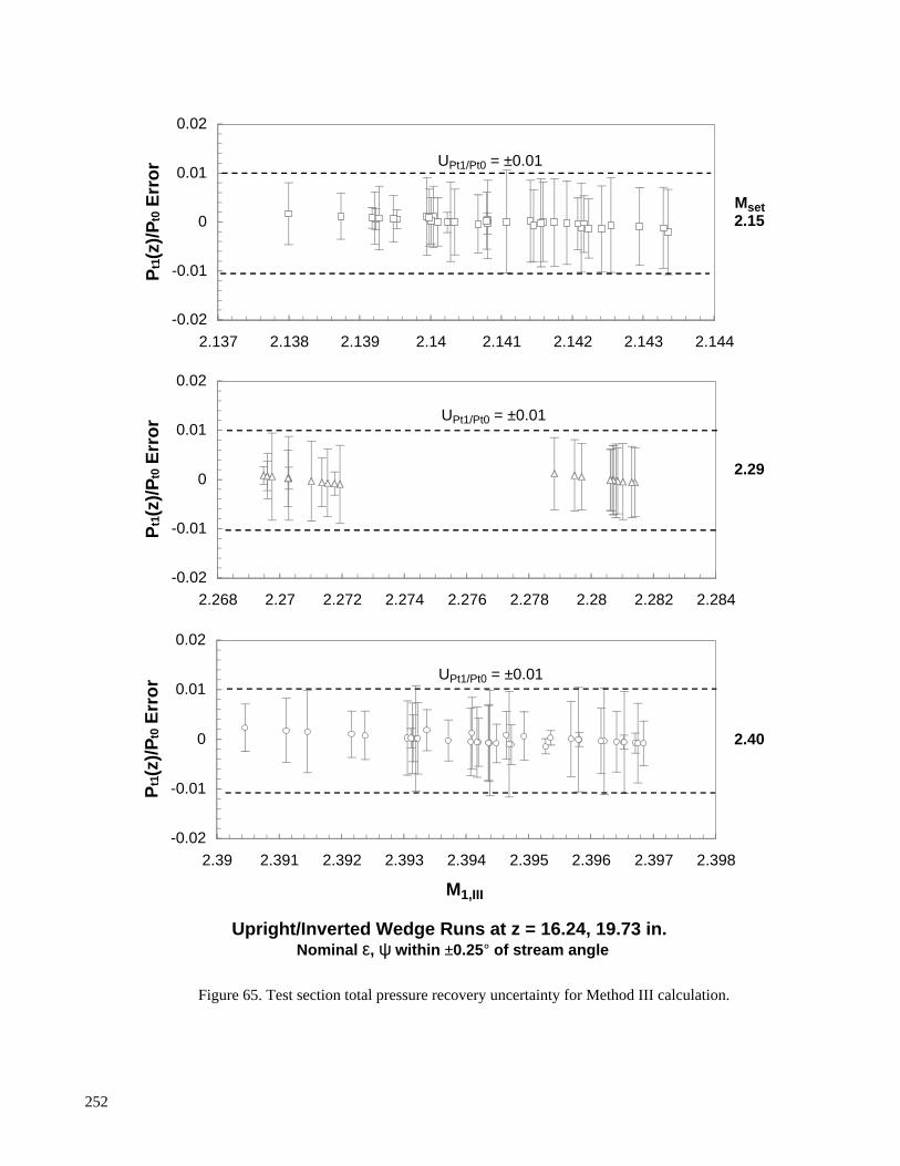
Figure 65. Test section total pressure recovery uncertainty for Method III calculation.

-0.02

-0.01

0

0.01

0.02

2.137 2.138 2.139 2.14 2.141 2.142 2.143 2.144

Pt1(z

)/P

t0 E

rro

r UPt1/Pt0 = ±0.01

-0.02

-0.01

0

0.01

0.02

2.268 2.27 2.272 2.274 2.276 2.278 2.28 2.282 2.284

Pt1(z

)/P

t0 E

rro

r UPt1/Pt0 = ±0.01

-0.02

-0.01

0

0.01

0.02

2.39 2.391 2.392 2.393 2.394 2.395 2.396 2.397 2.398

M1,III

Pt1(z

)/P

t0 E

rro

r UPt1/Pt0 = ±0.01

Upright/Inverted Wedge Runs at z = 16.24, 19.73 in. Nominal ε, ψ within ±0.25° of stream angle

Mset2.15

2.29

2.40

252

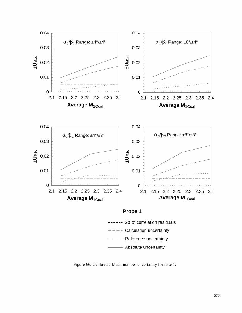
Figure 66. Calibrated Mach number uncertainty for rake 1.

0

0.01

0.02

0.03

0.04

2.1 2.15 2.2 2.25 2.3 2.35 2.4

Average M1Ccal

±UM

1c

αC/βC Range: ±4°/±4°

0

0.01

0.02

0.03

0.04

2.1 2.15 2.2 2.25 2.3 2.35 2.4

Average M1Ccal

±UM

1c

αC/βC Range: ±8°/±4°

0

0.01

0.02

0.03

0.04

2.1 2.15 2.2 2.25 2.3 2.35 2.4

Average M1Ccal

±UM

1c

αC/βC Range: ±4°/±8°

Probe 1

0

0.01

0.02

0.03

0.04

2.1 2.15 2.2 2.25 2.3 2.35 2.4Average M1Ccal

±UM

1c

αC/βC Range: ±8°/±8°

2σ of correlation residuals

Calculation uncertainty

Reference uncertainty

Absolute uncertainty

253

Figure 66. Continued.

0

0.01

0.02

0.03

0.04

2.1 2.15 2.2 2.25 2.3 2.35 2.4

Average M1Ccal

±UM

1c

αC/βC Range: ±4°/±4°

0

0.01

0.02

0.03

0.04

2.1 2.15 2.2 2.25 2.3 2.35 2.4

Average M1Ccal

±UM

1c

αC/βC Range: ±8°/±4°

0

0.01

0.02

0.03

0.04

2.1 2.15 2.2 2.25 2.3 2.35 2.4

Average M1Ccal

±UM

1c

αC/βC Range: ±4°/±8°

Probe 2

0

0.01

0.02

0.03

0.04

2.1 2.15 2.2 2.25 2.3 2.35 2.4Average M1Ccal

±UM

1c

αC/βC Range: ±8°/±8°

2σ of correlation residuals

Calculation uncertainty

Reference uncertainty

Absolute uncertainty

254

Figure 66. Continued.

0

0.01

0.02

0.03

0.04

2.1 2.15 2.2 2.25 2.3 2.35 2.4

Average M1Ccal

±UM

1c

αC/βC Range: ±4°/±4°

0

0.01

0.02

0.03

0.04

2.1 2.15 2.2 2.25 2.3 2.35 2.4

Average M1Ccal

±UM

1c

αC/βC Range: ±8°/±4°

0

0.01

0.02

0.03

0.04

2.1 2.15 2.2 2.25 2.3 2.35 2.4

Average M1Ccal

±UM

1c

αC/βC Range: ±4°/±8°

Probe 3

0

0.01

0.02

0.03

0.04

2.1 2.15 2.2 2.25 2.3 2.35 2.4Average M1Ccal

±UM

1c

αC/βC Range: ±8°/±8°

2σ of correlation residuals

Calculation uncertainty

Reference uncertainty

Absolute uncertainty

255

Figure 66. Continued.

0

0.01

0.02

0.03

0.04

2.1 2.15 2.2 2.25 2.3 2.35 2.4

Average M1Ccal

±UM

1c

αC/βC Range: ±4°/±4°

0

0.01

0.02

0.03

0.04

2.1 2.15 2.2 2.25 2.3 2.35 2.4

Average M1Ccal

±UM

1c

αC/βC Range: ±8°/±4°

0

0.01

0.02

0.03

0.04

2.1 2.15 2.2 2.25 2.3 2.35 2.4

Average M1Ccal

±UM

1c

αC/βC Range: ±4°/±8°

Probe 4

0

0.01

0.02

0.03

0.04

2.1 2.15 2.2 2.25 2.3 2.35 2.4Average M1Ccal

±UM

1c

αC/βC Range: ±8°/±8°

2σ of correlation residuals

Calculation uncertainty

Reference uncertainty

Absolute uncertainty

256

Figure 66. Continued.

0

0.01

0.02

0.03

0.04

2.1 2.15 2.2 2.25 2.3 2.35 2.4

Average M1Ccal

±UM

1c

αC/βC Range: ±4°/±4°

0

0.01

0.02

0.03

0.04

2.1 2.15 2.2 2.25 2.3 2.35 2.4

Average M1Ccal

±UM

1c

αC/βC Range: ±8°/±4°

0

0.01

0.02

0.03

0.04

2.1 2.15 2.2 2.25 2.3 2.35 2.4

Average M1Ccal

±UM

1c

αC/βC Range: ±4°/±8°

Probe 5

0

0.01

0.02

0.03

0.04

2.1 2.15 2.2 2.25 2.3 2.35 2.4Average M1Ccal

±UM

1c

αC/βC Range: ±8°/±8°

2σ of correlation residuals

Calculation uncertainty

Reference uncertainty

Absolute uncertainty

257

Figure 66. Continued.

0

0.01

0.02

0.03

0.04

2.1 2.15 2.2 2.25 2.3 2.35 2.4

Average M1Ccal

±UM

1c

αC/βC Range: ±4°/±4°

0

0.01

0.02

0.03

0.04

2.1 2.15 2.2 2.25 2.3 2.35 2.4

Average M1Ccal

±UM

1c

αC/βC Range: ±8°/±4°

0

0.01

0.02

0.03

0.04

2.1 2.15 2.2 2.25 2.3 2.35 2.4

Average M1Ccal

±UM

1c

αC/βC Range: ±4°/±8°

Probe 6

0

0.01

0.02

0.03

0.04

2.1 2.15 2.2 2.25 2.3 2.35 2.4Average M1Ccal

±UM

1c

αC/βC Range: ±8°/±8°

2σ of correlation residuals

Calculation uncertainty

Reference uncertainty

Absolute uncertainty

258

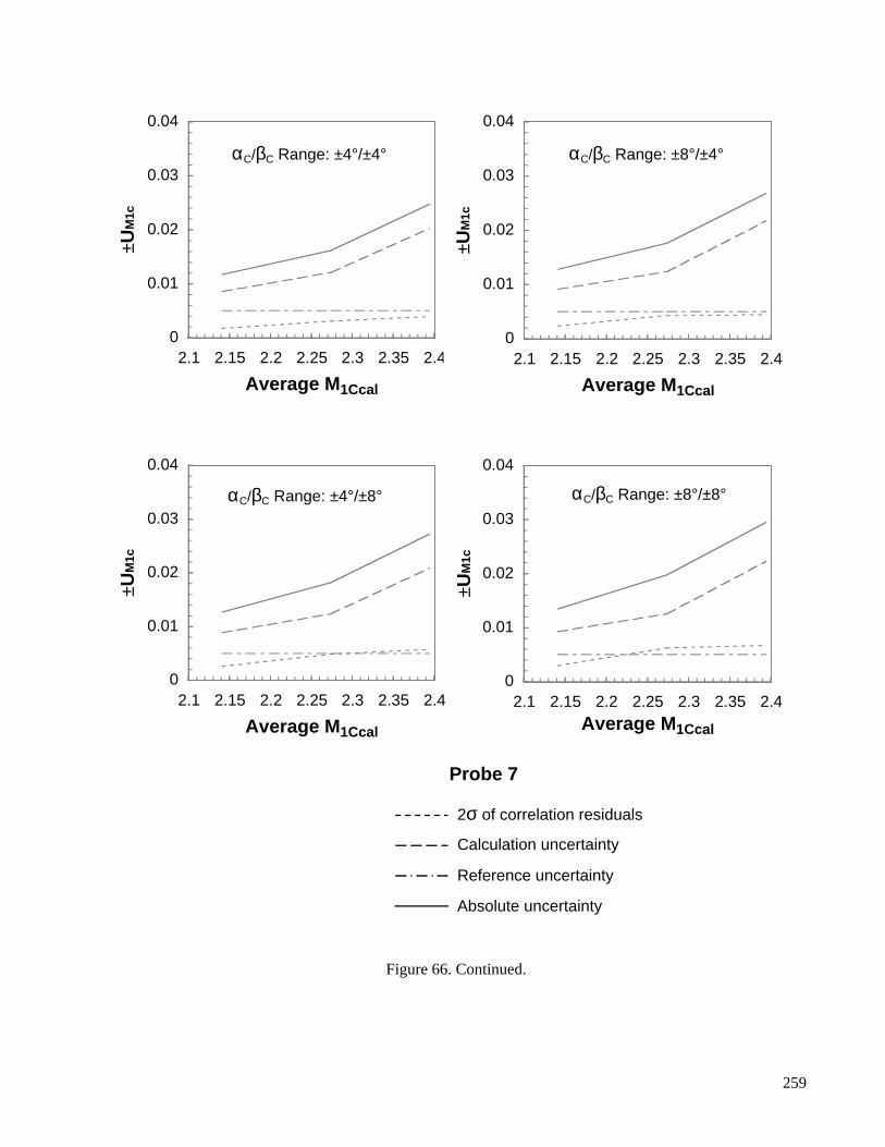
Figure 66. Continued.

0

0.01

0.02

0.03

0.04

2.1 2.15 2.2 2.25 2.3 2.35 2.4

Average M1Ccal

±UM

1c

αC/βC Range: ±4°/±4°

0

0.01

0.02

0.03

0.04

2.1 2.15 2.2 2.25 2.3 2.35 2.4

Average M1Ccal

±UM

1c

αC/βC Range: ±8°/±4°

0

0.01

0.02

0.03

0.04

2.1 2.15 2.2 2.25 2.3 2.35 2.4

Average M1Ccal

±UM

1c

αC/βC Range: ±4°/±8°

Probe 7

0

0.01

0.02

0.03

0.04

2.1 2.15 2.2 2.25 2.3 2.35 2.4Average M1Ccal

±UM

1c

αC/βC Range: ±8°/±8°

2σ of correlation residuals

Calculation uncertainty

Reference uncertainty

Absolute uncertainty

259

Figure 66. Concluded.

0

0.01

0.02

0.03

0.04

2.1 2.15 2.2 2.25 2.3 2.35 2.4

Average M1Ccal

±UM

1c

αC/βC Range: ±4°/±4°

0

0.01

0.02

0.03

0.04

2.1 2.15 2.2 2.25 2.3 2.35 2.4

Average M1Ccal

±UM

1c

αC/βC Range: ±8°/±4°

0

0.01

0.02

0.03

0.04

2.1 2.15 2.2 2.25 2.3 2.35 2.4

Average M1Ccal

±UM

1c

αC/βC Range: ±4°/±8°

Probe 8

0

0.01

0.02

0.03

0.04

2.1 2.15 2.2 2.25 2.3 2.35 2.4Average M1Ccal

±UM

1c

αC/βC Range: ±8°/±8°

2σ of correlation residuals

Calculation uncertainty

Reference uncertainty

Absolute uncertainty

260

Figure 67. Calibrated Mach number uncertainty for rake 2.

0

0.01

0.02

0.03

0.04

2.1 2.15 2.2 2.25 2.3 2.35 2.4

Average M1Ccal

±UM

1c

αC/βC Range: ±4°/±4°

0

0.01

0.02

0.03

0.04

2.1 2.15 2.2 2.25 2.3 2.35 2.4

Average M1Ccal

±UM

1c

αC/βC Range: ±8°/±4°

0

0.01

0.02

0.03

0.04

2.1 2.15 2.2 2.25 2.3 2.35 2.4

Average M1Ccal

±UM

1c

αC/βC Range: ±4°/±8°

Probe 1

0

0.01

0.02

0.03

0.04

2.1 2.15 2.2 2.25 2.3 2.35 2.4Average M1Ccal

±UM

1c

αC/βC Range: ±8°/±8°

2σ of correlation residuals

Calculation uncertainty

Reference uncertainty

Absolute uncertainty

261

Figure 67. Continued.

0

0.01

0.02

0.03

0.04

2.1 2.15 2.2 2.25 2.3 2.35 2.4

Average M1Ccal

±UM

1c

αC/βC Range: ±4°/±4°

0

0.01

0.02

0.03

0.04

2.1 2.15 2.2 2.25 2.3 2.35 2.4

Average M1Ccal

±UM

1c

αC/βC Range: ±8°/±4°

0

0.01

0.02

0.03

0.04

2.1 2.15 2.2 2.25 2.3 2.35 2.4

Average M1Ccal

±UM

1c

αC/βC Range: ±4°/±8°

Probe 2

0

0.01

0.02

0.03

0.04

2.1 2.15 2.2 2.25 2.3 2.35 2.4Average M1Ccal

±UM

1c

αC/βC Range: ±8°/±8°

2σ of correlation residuals

Calculation uncertainty

Reference uncertainty

Absolute uncertainty

262

Figure 67. Continued.

0

0.01

0.02

0.03

0.04

2.1 2.15 2.2 2.25 2.3 2.35 2.4

Average M1Ccal

±UM

1c

αC/βC Range: ±4°/±4°

0

0.01

0.02

0.03

0.04

2.1 2.15 2.2 2.25 2.3 2.35 2.4

Average M1Ccal

±UM

1c

αC/βC Range: ±8°/±4°

0

0.01

0.02

0.03

0.04

2.1 2.15 2.2 2.25 2.3 2.35 2.4

Average M1Ccal

±UM

1c

αC/βC Range: ±4°/±8°

Probe 3

0

0.01

0.02

0.03

0.04

2.1 2.15 2.2 2.25 2.3 2.35 2.4Average M1Ccal

±UM

1c

αC/βC Range: ±8°/±8°

2σ of correlation residuals

Calculation uncertainty

Reference uncertainty

Absolute uncertainty

263

Figure 67. Continued.

0

0.01

0.02

0.03

0.04

2.1 2.15 2.2 2.25 2.3 2.35 2.4

Average M1Ccal

±UM

1c

αC/βC Range: ±4°/±4°

0

0.01

0.02

0.03

0.04

2.1 2.15 2.2 2.25 2.3 2.35 2.4

Average M1Ccal

±UM

1c

αC/βC Range: ±8°/±4°

0

0.01

0.02

0.03

0.04

2.1 2.15 2.2 2.25 2.3 2.35 2.4

Average M1Ccal

±UM

1c

αC/βC Range: ±4°/±8°

Probe 4

0

0.01

0.02

0.03

0.04

2.1 2.15 2.2 2.25 2.3 2.35 2.4Average M1Ccal

±UM

1c

αC/βC Range: ±8°/±8°

2σ of correlation residuals

Calculation uncertainty

Reference uncertainty

Absolute uncertainty

264

Figure 67. Continued.

0

0.01

0.02

0.03

0.04

2.1 2.15 2.2 2.25 2.3 2.35 2.4

Average M1Ccal

±UM

1c

αC/βC Range: ±4°/±4°

0

0.01

0.02

0.03

0.04

2.1 2.15 2.2 2.25 2.3 2.35 2.4

Average M1Ccal

±UM

1c

αC/βC Range: ±8°/±4°

0

0.01

0.02

0.03

0.04

2.1 2.15 2.2 2.25 2.3 2.35 2.4

Average M1Ccal

±UM

1c

αC/βC Range: ±4°/±8°

Probe 5

0

0.01

0.02

0.03

0.04

2.1 2.15 2.2 2.25 2.3 2.35 2.4Average M1Ccal

±UM

1c

αC/βC Range: ±8°/±8°

2σ of correlation residuals

Calculation uncertainty

Reference uncertainty

Absolute uncertainty

265

Figure 67. Concluded.

0

0.01

0.02

0.03

0.04

2.1 2.15 2.2 2.25 2.3 2.35 2.4

Average M1Ccal

±UM

1c

αC/βC Range: ±4°/±4°

0

0.01

0.02

0.03

0.04

2.1 2.15 2.2 2.25 2.3 2.35 2.4

Average M1Ccal

±UM

1c

αC/βC Range: ±8°/±4°

0

0.01

0.02

0.03

0.04

2.1 2.15 2.2 2.25 2.3 2.35 2.4

Average M1Ccal

±UM

1c

αC/βC Range: ±4°/±8°

Probe 6

0

0.01

0.02

0.03

0.04

2.1 2.15 2.2 2.25 2.3 2.35 2.4Average M1Ccal

±UM

1c

αC/βC Range: ±8°/±8°

2σ of correlation residuals

Calculation uncertainty

Reference uncertainty

Absolute uncertainty

266

Figure 68. Calibrated total pressure uncertainty for rake 1.

0

0.02

0.04

0.06

0.08

0.1

2.1 2.15 2.2 2.25 2.3 2.35 2.4

Average M1Ccal

±UP

t1c/

Pt0

αC/βC Range: ±4°/±4°

0

0.02

0.04

0.06

0.08

0.1

2.1 2.15 2.2 2.25 2.3 2.35 2.4

Average M1Ccal

±UP

t1c/

Pt0

αC/βC Range: ±8°/±4°

0

0.02

0.04

0.06

0.08

0.1

2.1 2.15 2.2 2.25 2.3 2.35 2.4

Average M1Ccal

±UP

t1c/

Pt0

αC/βC Range: ±4°/±8°

Probe 1

0

0.02

0.04

0.06

0.08

0.1

2.1 2.15 2.2 2.25 2.3 2.35 2.4Average M1Ccal

±UP

t1c/

Pt0

αC/βC Range: ±8°/±8°

2σ of correlation residuals

Calculation uncertainty

Reference uncertainty

Absolute uncertainty

267

Figure 68. Continued.

0

0.02

0.04

0.06

0.08

0.1

2.1 2.15 2.2 2.25 2.3 2.35 2.4

Average M1Ccal

±UP

t1c/

Pt0

αC/βC Range: ±4°/±4°

0

0.02

0.04

0.06

0.08

0.1

2.1 2.15 2.2 2.25 2.3 2.35 2.4

Average M1Ccal

±UP

t1c/

Pt0

αC/βC Range: ±8°/±4°

0

0.02

0.04

0.06

0.08

0.1

2.1 2.15 2.2 2.25 2.3 2.35 2.4

Average M1Ccal

±UP

t1c/

Pt0

αC/βC Range: ±4°/±8°

Probe 2

0

0.02

0.04

0.06

0.08

0.1

2.1 2.15 2.2 2.25 2.3 2.35 2.4Average M1Ccal

±UP

t1c/

Pt0

αC/βC Range: ±8°/±8°

2σ of correlation residuals

Calculation uncertainty

Reference uncertainty

Absolute uncertainty

268

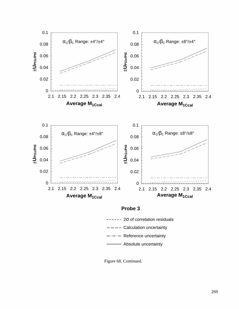
Figure 68. Continued.

0

0.02

0.04

0.06

0.08

0.1

2.1 2.15 2.2 2.25 2.3 2.35 2.4

Average M1Ccal

±UP

t1c/

Pt0

αC/βC Range: ±4°/±4°

0

0.02

0.04

0.06

0.08

0.1

2.1 2.15 2.2 2.25 2.3 2.35 2.4

Average M1Ccal

±UP

t1c/

Pt0

αC/βC Range: ±8°/±4°

0

0.02

0.04

0.06

0.08

0.1

2.1 2.15 2.2 2.25 2.3 2.35 2.4

Average M1Ccal

±UP

t1c/

Pt0

αC/βC Range: ±4°/±8°

Probe 3

0

0.02

0.04

0.06

0.08

0.1

2.1 2.15 2.2 2.25 2.3 2.35 2.4Average M1Ccal

±UP

t1c/

Pt0

αC/βC Range: ±8°/±8°

2σ of correlation residuals

Calculation uncertainty

Reference uncertainty

Absolute uncertainty

269

Figure 68. Continued.

0

0.02

0.04

0.06

0.08

0.1

2.1 2.15 2.2 2.25 2.3 2.35 2.4

Average M1Ccal

±UP

t1c/

Pt0

αC/βC Range: ±4°/±4°

0

0.02

0.04

0.06

0.08

0.1

2.1 2.15 2.2 2.25 2.3 2.35 2.4

Average M1Ccal

±UP

t1c/

Pt0

αC/βC Range: ±8°/±4°

0

0.02

0.04

0.06

0.08

0.1

2.1 2.15 2.2 2.25 2.3 2.35 2.4

Average M1Ccal

±UP

t1c/

Pt0

αC/βC Range: ±4°/±8°

Probe 4

0

0.02

0.04

0.06

0.08

0.1

2.1 2.15 2.2 2.25 2.3 2.35 2.4Average M1Ccal

±UP

t1c/

Pt0

αC/βC Range: ±8°/±8°

2σ of correlation residuals

Calculation uncertainty

Reference uncertainty

Absolute uncertainty

270

Figure 68. Continued.

0

0.02

0.04

0.06

0.08

0.1

2.1 2.15 2.2 2.25 2.3 2.35 2.4

Average M1Ccal

±UP

t1c/

Pt0

αC/βC Range: ±4°/±4°

0

0.02

0.04

0.06

0.08

0.1

2.1 2.15 2.2 2.25 2.3 2.35 2.4

Average M1Ccal

±UP

t1c/

Pt0

αC/βC Range: ±8°/±4°

0

0.02

0.04

0.06

0.08

0.1

2.1 2.15 2.2 2.25 2.3 2.35 2.4

Average M1Ccal

±UP

t1c/

Pt0

αC/βC Range: ±4°/±8°

Probe 5

0

0.02

0.04

0.06

0.08

0.1

2.1 2.15 2.2 2.25 2.3 2.35 2.4Average M1Ccal

±UP

t1c/

Pt0

αC/βC Range: ±8°/±8°

2σ of correlation residuals

Calculation uncertainty

Reference uncertainty

Absolute uncertainty

271

Figure 68. Continued.

0

0.02

0.04

0.06

0.08

0.1

2.1 2.15 2.2 2.25 2.3 2.35 2.4

Average M1Ccal

±UP

t1c/

Pt0

αC/βC Range: ±4°/±4°

0

0.02

0.04

0.06

0.08

0.1

2.1 2.15 2.2 2.25 2.3 2.35 2.4

Average M1Ccal

±UP

t1c/

Pt0

αC/βC Range: ±8°/±4°

0

0.02

0.04

0.06

0.08

0.1

2.1 2.15 2.2 2.25 2.3 2.35 2.4

Average M1Ccal

±UP

t1c/

Pt0

αC/βC Range: ±4°/±8°

Probe 6

0

0.02

0.04

0.06

0.08

0.1

2.1 2.15 2.2 2.25 2.3 2.35 2.4Average M1Ccal

±UP

t1c/

Pt0

αC/βC Range: ±8°/±8°

2σ of correlation residuals

Calculation uncertainty

Reference uncertainty

Absolute uncertainty

272

Figure 68. Continued.

0

0.02

0.04

0.06

0.08

0.1

2.1 2.15 2.2 2.25 2.3 2.35 2.4

Average M1Ccal

±UP

t1c/

Pt0

αC/βC Range: ±4°/±4°

0

0.02

0.04

0.06

0.08

0.1

2.1 2.15 2.2 2.25 2.3 2.35 2.4

Average M1Ccal

±UP

t1c/

Pt0

αC/βC Range: ±8°/±4°

0

0.02

0.04

0.06

0.08

0.1

2.1 2.15 2.2 2.25 2.3 2.35 2.4

Average M1Ccal

±UP

t1c/

Pt0

αC/βC Range: ±4°/±8°

Probe 7

0

0.02

0.04

0.06

0.08

0.1

2.1 2.15 2.2 2.25 2.3 2.35 2.4Average M1Ccal

±UP

t1c/

Pt0

αC/βC Range: ±8°/±8°

2σ of correlation residuals

Calculation uncertainty

Reference uncertainty

Absolute uncertainty

273

Figure 68. Concluded.

0

0.02

0.04

0.06

0.08

0.1

2.1 2.15 2.2 2.25 2.3 2.35 2.4

Average M1Ccal

±UP

t1c/

Pt0

αC/βC Range: ±4°/±4°

0

0.02

0.04

0.06

0.08

0.1

2.1 2.15 2.2 2.25 2.3 2.35 2.4

Average M1Ccal

±UP

t1c/

Pt0

αC/βC Range: ±8°/±4°

0

0.02

0.04

0.06

0.08

0.1

2.1 2.15 2.2 2.25 2.3 2.35 2.4

Average M1Ccal

±UP

t1c/

Pt0

αC/βC Range: ±4°/±8°

Probe 8

0

0.02

0.04

0.06

0.08

0.1

2.1 2.15 2.2 2.25 2.3 2.35 2.4Average M1Ccal

±UP

t1c/

Pt0

αC/βC Range: ±8°/±8°

2σ of correlation residuals

Calculation uncertainty

Reference uncertainty

Absolute uncertainty

274

Figure 69. Calibrated total pressure uncertainty for rake 2.

0

0.02

0.04

0.06

0.08

0.1

2.1 2.15 2.2 2.25 2.3 2.35 2.4

Average M1Ccal

±UP

t1c/

Pt0

αC/βC Range: ±4°/±4°

0

0.02

0.04

0.06

0.08

0.1

2.1 2.15 2.2 2.25 2.3 2.35 2.4

Average M1Ccal

±UP

t1c/

Pt0

αC/βC Range: ±8°/±4°

0

0.02

0.04

0.06

0.08

0.1

2.1 2.15 2.2 2.25 2.3 2.35 2.4

Average M1Ccal

±UP

t1c/

Pt0

αC/βC Range: ±4°/±8°

Probe 1

0

0.02

0.04

0.06

0.08

0.1

2.1 2.15 2.2 2.25 2.3 2.35 2.4Average M1Ccal

±UP

t1c/

Pt0

αC/βC Range: ±8°/±8°

2σ of correlation residuals

Calculation uncertainty

Reference uncertainty

Absolute uncertainty

275

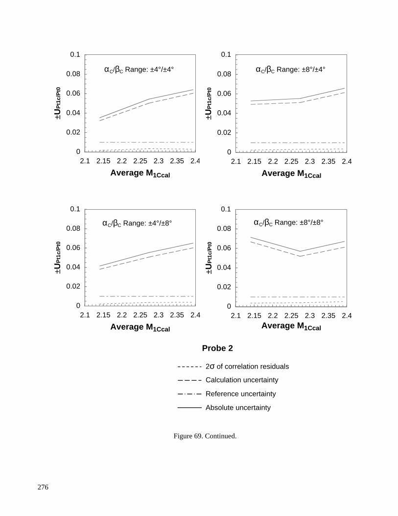
Figure 69. Continued.

0

0.02

0.04

0.06

0.08

0.1

2.1 2.15 2.2 2.25 2.3 2.35 2.4

Average M1Ccal

±UP

t1c/

Pt0

αC/βC Range: ±4°/±4°

0

0.02

0.04

0.06

0.08

0.1

2.1 2.15 2.2 2.25 2.3 2.35 2.4

Average M1Ccal

±UP

t1c/

Pt0

αC/βC Range: ±8°/±4°

0

0.02

0.04

0.06

0.08

0.1

2.1 2.15 2.2 2.25 2.3 2.35 2.4

Average M1Ccal

±UP

t1c/

Pt0

αC/βC Range: ±4°/±8°

Probe 2

0

0.02

0.04

0.06

0.08

0.1

2.1 2.15 2.2 2.25 2.3 2.35 2.4Average M1Ccal

±UP

t1c/

Pt0

αC/βC Range: ±8°/±8°

2σ of correlation residuals

Calculation uncertainty

Reference uncertainty

Absolute uncertainty

276

Figure 69. Continued.

0

0.02

0.04

0.06

0.08

0.1

2.1 2.15 2.2 2.25 2.3 2.35 2.4

Average M1Ccal

±UP

t1c/

Pt0

αC/βC Range: ±4°/±4°

0

0.02

0.04

0.06

0.08

0.1

2.1 2.15 2.2 2.25 2.3 2.35 2.4

Average M1Ccal

±UP

t1c/

Pt0

αC/βC Range: ±8°/±4°

0

0.02

0.04

0.06

0.08

0.1

2.1 2.15 2.2 2.25 2.3 2.35 2.4

Average M1Ccal

±UP

t1c/

Pt0

αC/βC Range: ±4°/±8°

Probe 3

0

0.02

0.04

0.06

0.08

0.1

2.1 2.15 2.2 2.25 2.3 2.35 2.4Average M1Ccal

±UP

t1c/

Pt0

αC/βC Range: ±8°/±8°

2σ of correlation residuals

Calculation uncertainty

Reference uncertainty

Absolute uncertainty

277

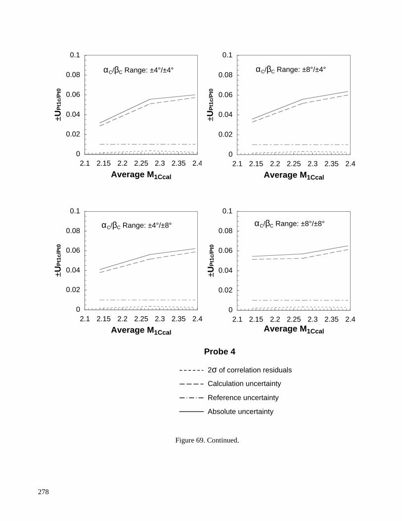
Figure 69. Continued.

0

0.02

0.04

0.06

0.08

0.1

2.1 2.15 2.2 2.25 2.3 2.35 2.4

Average M1Ccal

±UP

t1c/

Pt0

αC/βC Range: ±4°/±4°

0

0.02

0.04

0.06

0.08

0.1

2.1 2.15 2.2 2.25 2.3 2.35 2.4

Average M1Ccal

±UP

t1c/

Pt0

αC/βC Range: ±8°/±4°

0

0.02

0.04

0.06

0.08

0.1

2.1 2.15 2.2 2.25 2.3 2.35 2.4

Average M1Ccal

±UP

t1c/

Pt0

αC/βC Range: ±4°/±8°

Probe 4

0

0.02

0.04

0.06

0.08

0.1

2.1 2.15 2.2 2.25 2.3 2.35 2.4Average M1Ccal

±UP

t1c/

Pt0

αC/βC Range: ±8°/±8°

2σ of correlation residuals

Calculation uncertainty

Reference uncertainty

Absolute uncertainty

278

Figure 69. Continued.

0

0.02

0.04

0.06

0.08

0.1

2.1 2.15 2.2 2.25 2.3 2.35 2.4

Average M1Ccal

±UP

t1c/

Pt0

αC/βC Range: ±4°/±4°

0

0.02

0.04

0.06

0.08

0.1

2.1 2.15 2.2 2.25 2.3 2.35 2.4

Average M1Ccal

±UP

t1c/

Pt0

αC/βC Range: ±8°/±4°

0

0.02

0.04

0.06

0.08

0.1

2.1 2.15 2.2 2.25 2.3 2.35 2.4

Average M1Ccal

±UP

t1c/

Pt0

αC/βC Range: ±4°/±8°

Probe 5

0

0.02

0.04

0.06

0.08

0.1

2.1 2.15 2.2 2.25 2.3 2.35 2.4Average M1Ccal

±UP

t1c/

Pt0

αC/βC Range: ±8°/±8°

2σ of correlation residuals

Calculation uncertainty

Reference uncertainty

Absolute uncertainty

279

Figure 69. Concluded.

0

0.02

0.04

0.06

0.08

0.1

2.1 2.15 2.2 2.25 2.3 2.35 2.4

Average M1Ccal

±UP

t1c/

Pt0

αC/βC Range: ±4°/±4°

0

0.02

0.04

0.06

0.08

0.1

2.1 2.15 2.2 2.25 2.3 2.35 2.4

Average M1Ccal

±UP

t1c/

Pt0

αC/βC Range: ±8°/±4°

0

0.02

0.04

0.06

0.08

0.1

2.1 2.15 2.2 2.25 2.3 2.35 2.4

Average M1Ccal

±UP

t1c/

Pt0

αC/βC Range: ±4°/±8°

Probe 6

0

0.02

0.04

0.06

0.08

0.1

2.1 2.15 2.2 2.25 2.3 2.35 2.4Average M1Ccal

±UP

t1c/

Pt0

αC/βC Range: ±8°/±8°

2σ of correlation residuals

Calculation uncertainty

Reference uncertainty

Absolute uncertainty

280

Figure 70. Calibrated angle of attack uncertainty for rake 1.

0

0.05

0.1

0.15

0.2

0.25

0.3

2.1 2.15 2.2 2.25 2.3 2.35 2.4

Average M1Ccal

±Uαc

(d

eg)

αC/βC Range: ±4°/±4°

0

0.05

0.1

0.15

0.2

0.25

0.3

2.1 2.15 2.2 2.25 2.3 2.35 2.4

Average M1Ccal

±Uαc

(d

eg)

αC/βC Range: ±8°/±4°

0

0.05

0.1

0.15

0.2

0.25

0.3

2.1 2.15 2.2 2.25 2.3 2.35 2.4

Average M1Ccal

±Uαc

(d

eg)

αC/βC Range: ±4°/±8°

Probe 1

0

0.05

0.1

0.15

0.2

0.25

0.3

2.1 2.15 2.2 2.25 2.3 2.35 2.4Average M1Ccal

±Uαc

(d

eg)

αC/βC Range: ±8°/±8°

2σ of correlation residuals

Calculation uncertainty

Reference uncertainty

Absolute uncertainty

281

Figure 70. Continued.

0

0.05

0.1

0.15

0.2

0.25

0.3

2.1 2.15 2.2 2.25 2.3 2.35 2.4

Average M1Ccal

±Uαc

(d

eg)

αC/βC Range: ±4°/±4°

0

0.05

0.1

0.15

0.2

0.25

0.3

2.1 2.15 2.2 2.25 2.3 2.35 2.4

Average M1Ccal

±Uαc

(d

eg)

αC/βC Range: ±8°/±4°

0

0.05

0.1

0.15

0.2

0.25

0.3

2.1 2.15 2.2 2.25 2.3 2.35 2.4

Average M1Ccal

±Uαc

(d

eg)

αC/βC Range: ±4°/±8°

Probe 2

0

0.05

0.1

0.15

0.2

0.25

0.3

2.1 2.15 2.2 2.25 2.3 2.35 2.4Average M1Ccal

±Uαc

(d

eg)

αC/βC Range: ±8°/±8°

2σ of correlation residuals

Calculation uncertainty

Reference uncertainty

Absolute uncertainty

282

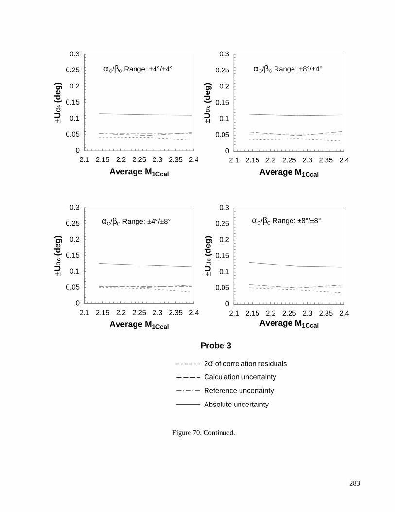
Figure 70. Continued.

0

0.05

0.1

0.15

0.2

0.25

0.3

2.1 2.15 2.2 2.25 2.3 2.35 2.4

Average M1Ccal

±Uαc

(d

eg)

αC/βC Range: ±4°/±4°

0

0.05

0.1

0.15

0.2

0.25

0.3

2.1 2.15 2.2 2.25 2.3 2.35 2.4

Average M1Ccal

±Uαc

(d

eg)

αC/βC Range: ±8°/±4°

0

0.05

0.1

0.15

0.2

0.25

0.3

2.1 2.15 2.2 2.25 2.3 2.35 2.4

Average M1Ccal

±Uαc

(d

eg)

αC/βC Range: ±4°/±8°

Probe 3

0

0.05

0.1

0.15

0.2

0.25

0.3

2.1 2.15 2.2 2.25 2.3 2.35 2.4Average M1Ccal

±Uαc

(d

eg)

αC/βC Range: ±8°/±8°

2σ of correlation residuals

Calculation uncertainty

Reference uncertainty

Absolute uncertainty

283

Figure 70. Continued.

0

0.05

0.1

0.15

0.2

0.25

0.3

2.1 2.15 2.2 2.25 2.3 2.35 2.4

Average M1Ccal

±Uαc

(d

eg)

αC/βC Range: ±4°/±4°

0

0.05

0.1

0.15

0.2

0.25

0.3

2.1 2.15 2.2 2.25 2.3 2.35 2.4

Average M1Ccal

±Uαc

(d

eg)

αC/βC Range: ±8°/±4°

0

0.05

0.1

0.15

0.2

0.25

0.3

2.1 2.15 2.2 2.25 2.3 2.35 2.4

Average M1Ccal

±Uαc

(d

eg)

αC/βC Range: ±4°/±8°

Probe 4

0

0.05

0.1

0.15

0.2

0.25

0.3

2.1 2.15 2.2 2.25 2.3 2.35 2.4Average M1Ccal

±Uαc

(d

eg)

αC/βC Range: ±8°/±8°

2σ of correlation residuals

Calculation uncertainty

Reference uncertainty

Absolute uncertainty

284

Figure 70. Continued.

0

0.05

0.1

0.15

0.2

0.25

0.3

2.1 2.15 2.2 2.25 2.3 2.35 2.4

Average M1Ccal

±Uαc

(d

eg)

αC/βC Range: ±4°/±4°

0

0.05

0.1

0.15

0.2

0.25

0.3

2.1 2.15 2.2 2.25 2.3 2.35 2.4

Average M1Ccal

±Uαc

(d

eg)

αC/βC Range: ±8°/±4°

0

0.05

0.1

0.15

0.2

0.25

0.3

2.1 2.15 2.2 2.25 2.3 2.35 2.4

Average M1Ccal

±Uαc

(d

eg)

αC/βC Range: ±4°/±8°

Probe 5

0

0.05

0.1

0.15

0.2

0.25

0.3

2.1 2.15 2.2 2.25 2.3 2.35 2.4Average M1Ccal

±Uαc

(d

eg)

αC/βC Range: ±8°/±8°

2σ of correlation residuals

Calculation uncertainty

Reference uncertainty

Absolute uncertainty

285

Figure 70. Continued.

0

0.05

0.1

0.15

0.2

0.25

0.3

2.1 2.15 2.2 2.25 2.3 2.35 2.4

Average M1Ccal

±Uαc

(d

eg)

αC/βC Range: ±4°/±4°

0

0.05

0.1

0.15

0.2

0.25

0.3

2.1 2.15 2.2 2.25 2.3 2.35 2.4

Average M1Ccal

±Uαc

(d

eg)

αC/βC Range: ±8°/±4°

0

0.05

0.1

0.15

0.2

0.25

0.3

2.1 2.15 2.2 2.25 2.3 2.35 2.4

Average M1Ccal

±Uαc

(d

eg)

αC/βC Range: ±4°/±8°

Probe 6

0

0.05

0.1

0.15

0.2

0.25

0.3

2.1 2.15 2.2 2.25 2.3 2.35 2.4Average M1Ccal

±Uαc

(d

eg)

αC/βC Range: ±8°/±8°

2σ of correlation residuals

Calculation uncertainty

Reference uncertainty

Absolute uncertainty

286

Figure 70. Continued.

0

0.05

0.1

0.15

0.2

0.25

0.3

2.1 2.15 2.2 2.25 2.3 2.35 2.4

Average M1Ccal

±Uαc

(d

eg)

αC/βC Range: ±4°/±4°

0

0.05

0.1

0.15

0.2

0.25

0.3

2.1 2.15 2.2 2.25 2.3 2.35 2.4

Average M1Ccal

±Uαc

(d

eg)

αC/βC Range: ±8°/±4°

0

0.05

0.1

0.15

0.2

0.25

0.3

2.1 2.15 2.2 2.25 2.3 2.35 2.4

Average M1Ccal

±Uαc

(d

eg)

αC/βC Range: ±4°/±8°

Probe 7

0

0.05

0.1

0.15

0.2

0.25

0.3

2.1 2.15 2.2 2.25 2.3 2.35 2.4Average M1Ccal

±Uαc

(d

eg)

αC/βC Range: ±8°/±8°

2σ of correlation residuals

Calculation uncertainty

Reference uncertainty

Absolute uncertainty

287

Figure 70. Concluded.

0

0.05

0.1

0.15

0.2

0.25

0.3

2.1 2.15 2.2 2.25 2.3 2.35 2.4

Average M1Ccal

±Uαc

(d

eg)

αC/βC Range: ±4°/±4°

0

0.05

0.1

0.15

0.2

0.25

0.3

2.1 2.15 2.2 2.25 2.3 2.35 2.4

Average M1Ccal

±Uαc

(d

eg)

αC/βC Range: ±8°/±4°

0

0.05

0.1

0.15

0.2

0.25

0.3

2.1 2.15 2.2 2.25 2.3 2.35 2.4

Average M1Ccal

±Uαc

(d

eg)

αC/βC Range: ±4°/±8°

Probe 8

0

0.05

0.1

0.15

0.2

0.25

0.3

2.1 2.15 2.2 2.25 2.3 2.35 2.4Average M1Ccal

±Uαc

(d

eg)

αC/βC Range: ±8°/±8°

2σ of correlation residuals

Calculation uncertainty

Reference uncertainty

Absolute uncertainty

288

Figure 71. Calibrated angle of attack uncertainty for rake 2.

0

0.05

0.1

0.15

0.2

0.25

0.3

2.1 2.15 2.2 2.25 2.3 2.35 2.4

Average M1Ccal

±Uαc

(d

eg)

αC/βC Range: ±4°/±4°

0

0.05

0.1

0.15

0.2

0.25

0.3

2.1 2.15 2.2 2.25 2.3 2.35 2.4

Average M1Ccal

±Uαc

(d

eg)

αC/βC Range: ±8°/±4°

0

0.05

0.1

0.15

0.2

0.25

0.3

2.1 2.15 2.2 2.25 2.3 2.35 2.4

Average M1Ccal

±Uαc

(d

eg)

αC/βC Range: ±4°/±8°

Probe 1

0

0.05

0.1

0.15

0.2

0.25

0.3

2.1 2.15 2.2 2.25 2.3 2.35 2.4Average M1Ccal

±Uαc

(d

eg)

αC/βC Range: ±8°/±8°

2σ of correlation residuals

Calculation uncertainty

Reference uncertainty

Absolute uncertainty

289

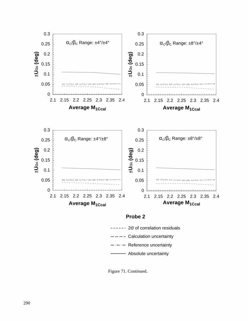
Figure 71. Continued.

0

0.05

0.1

0.15

0.2

0.25

0.3

2.1 2.15 2.2 2.25 2.3 2.35 2.4

Average M1Ccal

±Uαc

(d

eg)

αC/βC Range: ±4°/±4°

0

0.05

0.1

0.15

0.2

0.25

0.3

2.1 2.15 2.2 2.25 2.3 2.35 2.4

Average M1Ccal

±Uαc

(d

eg)

αC/βC Range: ±8°/±4°

0

0.05

0.1

0.15

0.2

0.25

0.3

2.1 2.15 2.2 2.25 2.3 2.35 2.4

Average M1Ccal

±Uαc

(d

eg)

αC/βC Range: ±4°/±8°

Probe 2

0

0.05

0.1

0.15

0.2

0.25

0.3

2.1 2.15 2.2 2.25 2.3 2.35 2.4Average M1Ccal

±Uαc

(d

eg)

αC/βC Range: ±8°/±8°

2σ of correlation residuals

Calculation uncertainty

Reference uncertainty

Absolute uncertainty

290

Figure 71. Continued.

0

0.05

0.1

0.15

0.2

0.25

0.3

2.1 2.15 2.2 2.25 2.3 2.35 2.4

Average M1Ccal

±Uαc

(d

eg)

αC/βC Range: ±4°/±4°

0

0.05

0.1

0.15

0.2

0.25

0.3

2.1 2.15 2.2 2.25 2.3 2.35 2.4

Average M1Ccal

±Uαc

(d

eg)

αC/βC Range: ±8°/±4°

0

0.05

0.1

0.15

0.2

0.25

0.3

2.1 2.15 2.2 2.25 2.3 2.35 2.4

Average M1Ccal

±Uαc

(d

eg)

αC/βC Range: ±4°/±8°

Probe 3

0

0.05

0.1

0.15

0.2

0.25

0.3

2.1 2.15 2.2 2.25 2.3 2.35 2.4Average M1Ccal

±Uαc

(d

eg)

αC/βC Range: ±8°/±8°

2σ of correlation residuals

Calculation uncertainty

Reference uncertainty

Absolute uncertainty

291

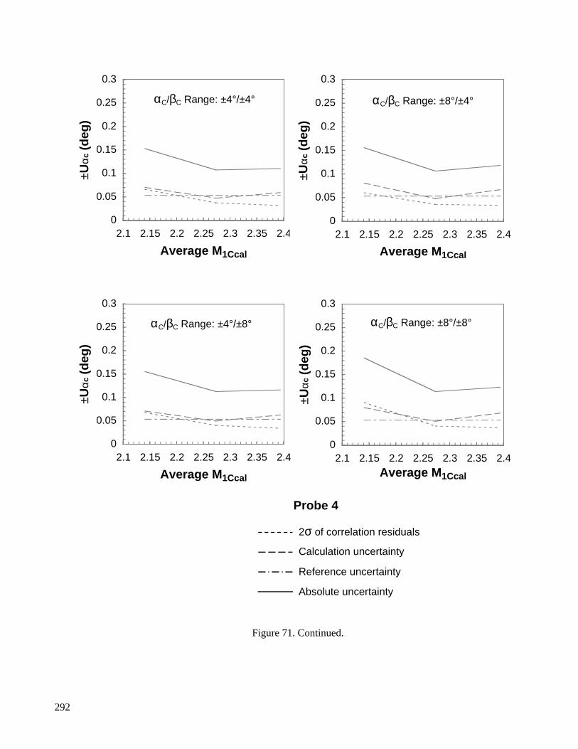
Figure 71. Continued.

0

0.05

0.1

0.15

0.2

0.25

0.3

2.1 2.15 2.2 2.25 2.3 2.35 2.4

Average M1Ccal

±Uαc

(d

eg)

αC/βC Range: ±4°/±4°

0

0.05

0.1

0.15

0.2

0.25

0.3

2.1 2.15 2.2 2.25 2.3 2.35 2.4

Average M1Ccal

±Uαc

(d

eg)

αC/βC Range: ±8°/±4°

0

0.05

0.1

0.15

0.2

0.25

0.3

2.1 2.15 2.2 2.25 2.3 2.35 2.4

Average M1Ccal

±Uαc

(d

eg)

αC/βC Range: ±4°/±8°

Probe 4

0

0.05

0.1

0.15

0.2

0.25

0.3

2.1 2.15 2.2 2.25 2.3 2.35 2.4Average M1Ccal

±Uαc

(d

eg)

αC/βC Range: ±8°/±8°

2σ of correlation residuals

Calculation uncertainty

Reference uncertainty

Absolute uncertainty

292

Figure 71. Continued.

0

0.05

0.1

0.15

0.2

0.25

0.3

2.1 2.15 2.2 2.25 2.3 2.35 2.4

Average M1Ccal

±Uαc

(d

eg)

αC/βC Range: ±4°/±4°

0

0.05

0.1

0.15

0.2

0.25

0.3

2.1 2.15 2.2 2.25 2.3 2.35 2.4

Average M1Ccal

±Uαc

(d

eg)

αC/βC Range: ±8°/±4°

0

0.05

0.1

0.15

0.2

0.25

0.3

2.1 2.15 2.2 2.25 2.3 2.35 2.4

Average M1Ccal

±Uαc

(d

eg)

αC/βC Range: ±4°/±8°

Probe 5

0

0.05

0.1

0.15

0.2

0.25

0.3

2.1 2.15 2.2 2.25 2.3 2.35 2.4Average M1Ccal

±Uαc

(d

eg)

αC/βC Range: ±8°/±8°

2σ of correlation residuals

Calculation uncertainty

Reference uncertainty

Absolute uncertainty

293

Figure 71. Concluded.

0

0.05

0.1

0.15

0.2

0.25

0.3

2.1 2.15 2.2 2.25 2.3 2.35 2.4

Average M1Ccal

±Uαc

(d

eg)

αC/βC Range: ±4°/±4°

0

0.05

0.1

0.15

0.2

0.25

0.3

2.1 2.15 2.2 2.25 2.3 2.35 2.4

Average M1Ccal

±Uαc

(d

eg)

αC/βC Range: ±8°/±4°

0

0.05

0.1

0.15

0.2

0.25

0.3

2.1 2.15 2.2 2.25 2.3 2.35 2.4

Average M1Ccal

±Uαc

(d

eg)

αC/βC Range: ±4°/±8°

Probe 6

0

0.05

0.1

0.15

0.2

0.25

0.3

2.1 2.15 2.2 2.25 2.3 2.35 2.4Average M1Ccal

±Uαc

(d

eg)

αC/βC Range: ±8°/±8°

2σ of correlation residuals

Calculation uncertainty

Reference uncertainty

Absolute uncertainty

294

Figure 72. Calibrated angle of sideslip uncertainty for rake 1.

0

0.05

0.1

0.15

0.2

0.25

0.3

2.1 2.15 2.2 2.25 2.3 2.35 2.4

Average M1Ccal

±Uβc

(d

eg)

αC/βC Range: ±4°/±4°

0

0.05

0.1

0.15

0.2

0.25

0.3

2.1 2.15 2.2 2.25 2.3 2.35 2.4

Average M1Ccal

±Uβc

(d

eg)

αC/βC Range: ±8°/±4°

0

0.05

0.1

0.15

0.2

0.25

0.3

2.1 2.15 2.2 2.25 2.3 2.35 2.4

Average M1Ccal

±Uβc

(d

eg)

αC/βC Range: ±4°/±8°

Probe 1

0

0.05

0.1

0.15

0.2

0.25

0.3

2.1 2.15 2.2 2.25 2.3 2.35 2.4Average M1Ccal

±Uβc

(d

eg)

αC/βC Range: ±8°/±8°

2σ of correlation residuals

Calculation uncertainty

Reference uncertainty

Absolute uncertainty

295

Figure 72. Continued.

0

0.05

0.1

0.15

0.2

0.25

0.3

2.1 2.15 2.2 2.25 2.3 2.35 2.4

Average M1Ccal

±Uβc

(d

eg)

αC/βC Range: ±4°/±4°

0

0.05

0.1

0.15

0.2

0.25

0.3

2.1 2.15 2.2 2.25 2.3 2.35 2.4

Average M1Ccal

±Uβc

(d

eg)

αC/βC Range: ±8°/±4°

0

0.05

0.1

0.15

0.2

0.25

0.3

2.1 2.15 2.2 2.25 2.3 2.35 2.4

Average M1Ccal

±Uβc

(d

eg)

αC/βC Range: ±4°/±8°

Probe 2

0

0.05

0.1

0.15

0.2

0.25

0.3

2.1 2.15 2.2 2.25 2.3 2.35 2.4Average M1Ccal

±Uβc

(d

eg)

αC/βC Range: ±8°/±8°

2σ of correlation residuals

Calculation uncertainty

Reference uncertainty

Absolute uncertainty

296

Figure 72. Continued.

0

0.05

0.1

0.15

0.2

0.25

0.3

2.1 2.15 2.2 2.25 2.3 2.35 2.4

Average M1Ccal

±Uβc

(d

eg)

αC/βC Range: ±4°/±4°

0

0.05

0.1

0.15

0.2

0.25

0.3

2.1 2.15 2.2 2.25 2.3 2.35 2.4

Average M1Ccal

±Uβc

(d

eg)

αC/βC Range: ±8°/±4°

0

0.05

0.1

0.15

0.2

0.25

0.3

2.1 2.15 2.2 2.25 2.3 2.35 2.4

Average M1Ccal

±Uβc

(d

eg)

αC/βC Range: ±4°/±8°

Probe 3

0

0.05

0.1

0.15

0.2

0.25

0.3

2.1 2.15 2.2 2.25 2.3 2.35 2.4Average M1Ccal

±Uβc

(d

eg)

αC/βC Range: ±8°/±8°

2σ of correlation residuals

Calculation uncertainty

Reference uncertainty

Absolute uncertainty

297

Figure 72. Continued.

0

0.05

0.1

0.15

0.2

0.25

0.3

2.1 2.15 2.2 2.25 2.3 2.35 2.4

Average M1Ccal

±Uβc

(d

eg)

αC/βC Range: ±4°/±4°

0

0.05

0.1

0.15

0.2

0.25

0.3

2.1 2.15 2.2 2.25 2.3 2.35 2.4

Average M1Ccal

±Uβc

(d

eg)

αC/βC Range: ±8°/±4°

0

0.05

0.1

0.15

0.2

0.25

0.3

2.1 2.15 2.2 2.25 2.3 2.35 2.4

Average M1Ccal

±Uβc

(d

eg)

αC/βC Range: ±4°/±8°

Probe 4

0

0.05

0.1

0.15

0.2

0.25

0.3

2.1 2.15 2.2 2.25 2.3 2.35 2.4Average M1Ccal

±Uβc

(d

eg)

αC/βC Range: ±8°/±8°

2σ of correlation residuals

Calculation uncertainty

Reference uncertainty

Absolute uncertainty

298

Figure 72. Continued.

0

0.05

0.1

0.15

0.2

0.25

0.3

2.1 2.15 2.2 2.25 2.3 2.35 2.4

Average M1Ccal

±Uβc

(d

eg)

αC/βC Range: ±4°/±4°

0

0.05

0.1

0.15

0.2

0.25

0.3

2.1 2.15 2.2 2.25 2.3 2.35 2.4

Average M1Ccal

±Uβc

(d

eg)

αC/βC Range: ±8°/±4°

0

0.05

0.1

0.15

0.2

0.25

0.3

2.1 2.15 2.2 2.25 2.3 2.35 2.4

Average M1Ccal

±Uβc

(d

eg)

αC/βC Range: ±4°/±8°

Probe 5

0

0.05

0.1

0.15

0.2

0.25

0.3

2.1 2.15 2.2 2.25 2.3 2.35 2.4Average M1Ccal

±Uβc

(d

eg)

αC/βC Range: ±8°/±8°

2σ of correlation residuals

Calculation uncertainty

Reference uncertainty

Absolute uncertainty

299

Figure 72. Continued.

0

0.05

0.1

0.15

0.2

0.25

0.3

2.1 2.15 2.2 2.25 2.3 2.35 2.4

Average M1Ccal

±Uβc

(d

eg)

αC/βC Range: ±4°/±4°

0

0.05

0.1

0.15

0.2

0.25

0.3

2.1 2.15 2.2 2.25 2.3 2.35 2.4

Average M1Ccal

±Uβc

(d

eg)

αC/βC Range: ±8°/±4°

0

0.05

0.1

0.15

0.2

0.25

0.3

2.1 2.15 2.2 2.25 2.3 2.35 2.4

Average M1Ccal

±Uβc

(d

eg)

αC/βC Range: ±4°/±8°

Probe 6

0

0.05

0.1

0.15

0.2

0.25

0.3

2.1 2.15 2.2 2.25 2.3 2.35 2.4Average M1Ccal

±Uβc

(d

eg)

αC/βC Range: ±8°/±8°

2σ of correlation residuals

Calculation uncertainty

Reference uncertainty

Absolute uncertainty

300

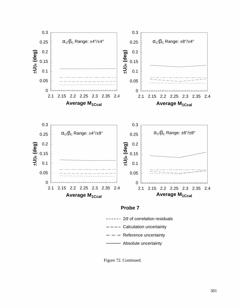
Figure 72. Continued.

0

0.05

0.1

0.15

0.2

0.25

0.3

2.1 2.15 2.2 2.25 2.3 2.35 2.4

Average M1Ccal

±Uβc

(d

eg)

αC/βC Range: ±4°/±4°

0

0.05

0.1

0.15

0.2

0.25

0.3

2.1 2.15 2.2 2.25 2.3 2.35 2.4

Average M1Ccal

±Uβc

(d

eg)

αC/βC Range: ±8°/±4°

0

0.05

0.1

0.15

0.2

0.25

0.3

2.1 2.15 2.2 2.25 2.3 2.35 2.4

Average M1Ccal

±Uβc

(d

eg)

αC/βC Range: ±4°/±8°

Probe 7

0

0.05

0.1

0.15

0.2

0.25

0.3

2.1 2.15 2.2 2.25 2.3 2.35 2.4Average M1Ccal

±Uβc

(d

eg)

αC/βC Range: ±8°/±8°

2σ of correlation residuals

Calculation uncertainty

Reference uncertainty

Absolute uncertainty

301

Figure 72. Concluded.

0

0.05

0.1

0.15

0.2

0.25

0.3

2.1 2.15 2.2 2.25 2.3 2.35 2.4

Average M1Ccal

±Uβc

(d

eg)

αC/βC Range: ±4°/±4°

0

0.05

0.1

0.15

0.2

0.25

0.3

2.1 2.15 2.2 2.25 2.3 2.35 2.4

Average M1Ccal

±Uβc

(d

eg)

αC/βC Range: ±8°/±4°

0

0.05

0.1

0.15

0.2

0.25

0.3

2.1 2.15 2.2 2.25 2.3 2.35 2.4

Average M1Ccal

±Uβc

(d

eg)

αC/βC Range: ±4°/±8°

Probe 8

0

0.05

0.1

0.15

0.2

0.25

0.3

2.1 2.15 2.2 2.25 2.3 2.35 2.4Average M1Ccal

±Uβc

(d

eg)

αC/βC Range: ±8°/±8°

2σ of correlation residuals

Calculation uncertainty

Reference uncertainty

Absolute uncertainty

302

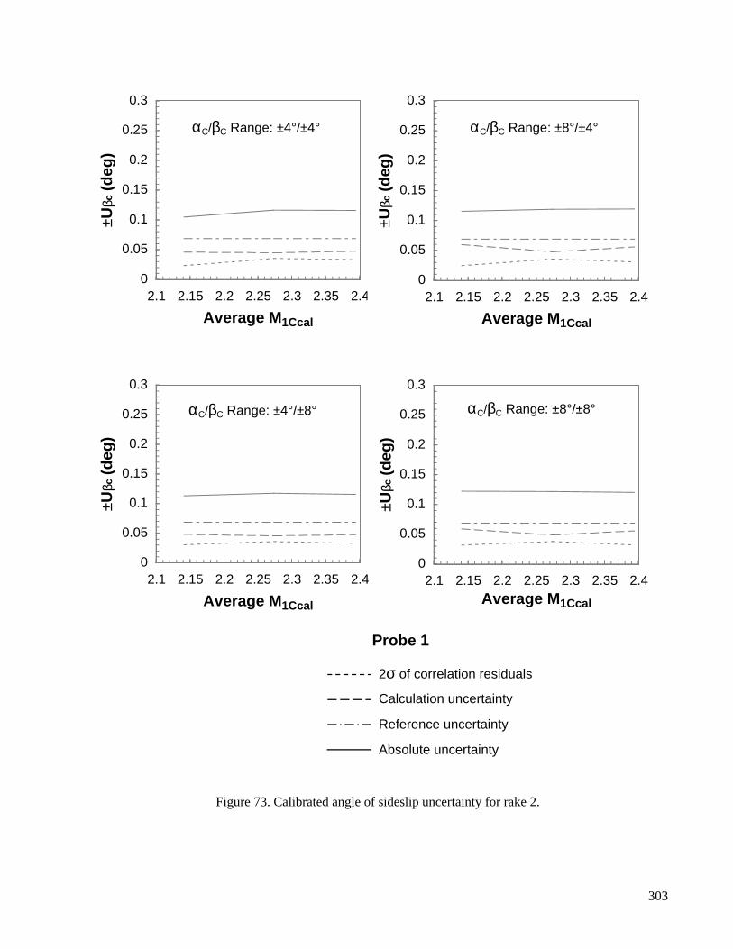
Figure 73. Calibrated angle of sideslip uncertainty for rake 2.

0

0.05

0.1

0.15

0.2

0.25

0.3

2.1 2.15 2.2 2.25 2.3 2.35 2.4

Average M1Ccal

±Uβc

(d

eg)

αC/βC Range: ±4°/±4°

0

0.05

0.1

0.15

0.2

0.25

0.3

2.1 2.15 2.2 2.25 2.3 2.35 2.4

Average M1Ccal

±Uβc

(d

eg)

αC/βC Range: ±8°/±4°

0

0.05

0.1

0.15

0.2

0.25

0.3

2.1 2.15 2.2 2.25 2.3 2.35 2.4

Average M1Ccal

±Uβc

(d

eg)

αC/βC Range: ±4°/±8°

Probe 1

0

0.05

0.1

0.15

0.2

0.25

0.3

2.1 2.15 2.2 2.25 2.3 2.35 2.4Average M1Ccal

±Uβc

(d

eg)

αC/βC Range: ±8°/±8°

2σ of correlation residuals

Calculation uncertainty

Reference uncertainty

Absolute uncertainty

303

Figure 73. Continued.

0

0.05

0.1

0.15

0.2

0.25

0.3

2.1 2.15 2.2 2.25 2.3 2.35 2.4

Average M1Ccal

±Uβc

(d

eg)

αC/βC Range: ±4°/±4°

0

0.05

0.1

0.15

0.2

0.25

0.3

2.1 2.15 2.2 2.25 2.3 2.35 2.4

Average M1Ccal

±Uβc

(d

eg)

αC/βC Range: ±8°/±4°

0

0.05

0.1

0.15

0.2

0.25

0.3

2.1 2.15 2.2 2.25 2.3 2.35 2.4

Average M1Ccal

±Uβc

(d

eg)

αC/βC Range: ±4°/±8°

Probe 2

0

0.05

0.1

0.15

0.2

0.25

0.3

2.1 2.15 2.2 2.25 2.3 2.35 2.4Average M1Ccal

±Uβc

(d

eg)

αC/βC Range: ±8°/±8°

2σ of correlation residuals

Calculation uncertainty

Reference uncertainty

Absolute uncertainty

304

Figure 73. Continued.

0

0.05

0.1

0.15

0.2

0.25

0.3

2.1 2.15 2.2 2.25 2.3 2.35 2.4

Average M1Ccal

±Uβc

(d

eg)

αC/βC Range: ±4°/±4°

0

0.05

0.1

0.15

0.2

0.25

0.3

2.1 2.15 2.2 2.25 2.3 2.35 2.4

Average M1Ccal

±Uβc

(d

eg)

αC/βC Range: ±8°/±4°

0

0.05

0.1

0.15

0.2

0.25

0.3

2.1 2.15 2.2 2.25 2.3 2.35 2.4

Average M1Ccal

±Uβc

(d

eg)

αC/βC Range: ±4°/±8°

Probe 3

0

0.05

0.1

0.15

0.2

0.25

0.3

2.1 2.15 2.2 2.25 2.3 2.35 2.4Average M1Ccal

±Uβc

(d

eg)

αC/βC Range: ±8°/±8°

2σ of correlation residuals

Calculation uncertainty

Reference uncertainty

Absolute uncertainty

305

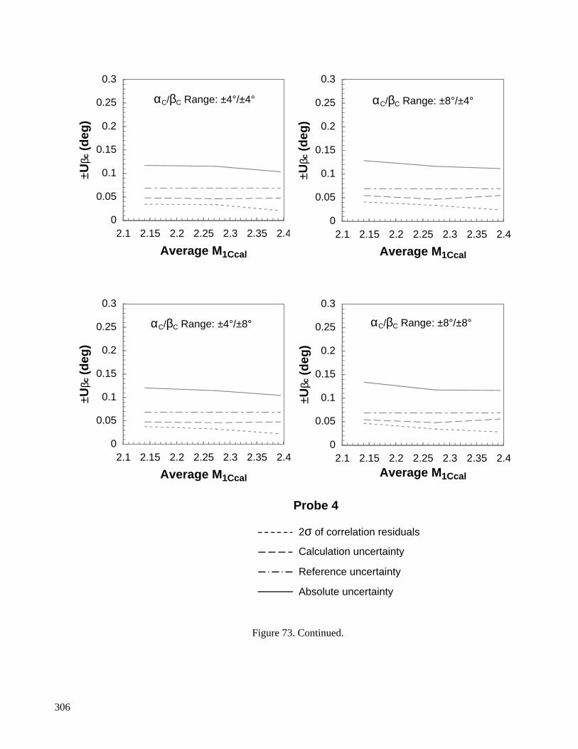
Figure 73. Continued.

0

0.05

0.1

0.15

0.2

0.25

0.3

2.1 2.15 2.2 2.25 2.3 2.35 2.4

Average M1Ccal

±Uβc

(d

eg)

αC/βC Range: ±4°/±4°

0

0.05

0.1

0.15

0.2

0.25

0.3

2.1 2.15 2.2 2.25 2.3 2.35 2.4

Average M1Ccal

±Uβc

(d

eg)

αC/βC Range: ±8°/±4°

0

0.05

0.1

0.15

0.2

0.25

0.3

2.1 2.15 2.2 2.25 2.3 2.35 2.4

Average M1Ccal

±Uβc

(d

eg)

αC/βC Range: ±4°/±8°

Probe 4

0

0.05

0.1

0.15

0.2

0.25

0.3

2.1 2.15 2.2 2.25 2.3 2.35 2.4Average M1Ccal

±Uβc

(d

eg)

αC/βC Range: ±8°/±8°

2σ of correlation residuals

Calculation uncertainty

Reference uncertainty

Absolute uncertainty

306

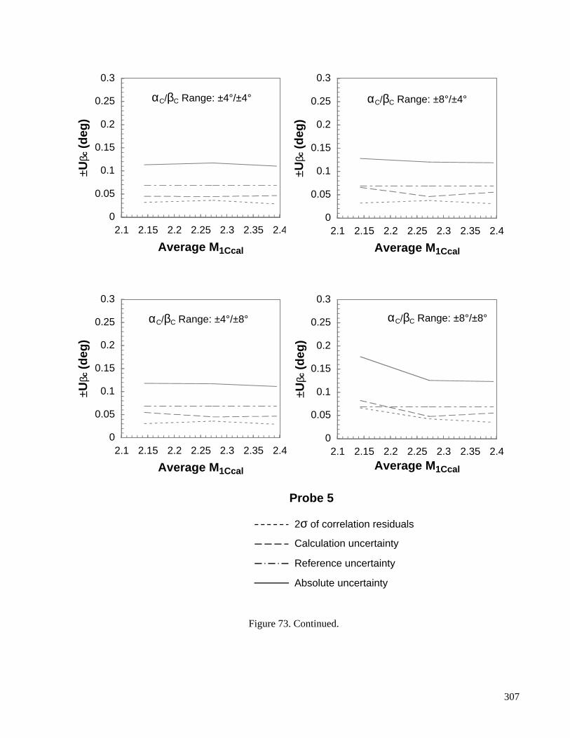
Figure 73. Continued.

0

0.05

0.1

0.15

0.2

0.25

0.3

2.1 2.15 2.2 2.25 2.3 2.35 2.4

Average M1Ccal

±Uβc

(d

eg)

αC/βC Range: ±4°/±4°

0

0.05

0.1

0.15

0.2

0.25

0.3

2.1 2.15 2.2 2.25 2.3 2.35 2.4

Average M1Ccal

±Uβc

(d

eg)

αC/βC Range: ±8°/±4°

0

0.05

0.1

0.15

0.2

0.25

0.3

2.1 2.15 2.2 2.25 2.3 2.35 2.4

Average M1Ccal

±Uβc

(d

eg)

αC/βC Range: ±4°/±8°

Probe 5

0

0.05

0.1

0.15

0.2

0.25

0.3

2.1 2.15 2.2 2.25 2.3 2.35 2.4Average M1Ccal

±Uβc

(d

eg)

αC/βC Range: ±8°/±8°

2σ of correlation residuals

Calculation uncertainty

Reference uncertainty

Absolute uncertainty

307

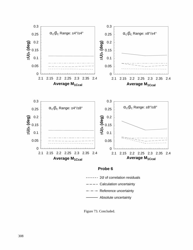
Figure 73. Concluded.

0

0.05

0.1

0.15

0.2

0.25

0.3

2.1 2.15 2.2 2.25 2.3 2.35 2.4

Average M1Ccal

±Uβc

(d

eg)

αC/βC Range: ±4°/±4°

0

0.05

0.1

0.15

0.2

0.25

0.3

2.1 2.15 2.2 2.25 2.3 2.35 2.4

Average M1Ccal

±Uβc

(d

eg)

αC/βC Range: ±8°/±4°

0

0.05

0.1

0.15

0.2

0.25

0.3

2.1 2.15 2.2 2.25 2.3 2.35 2.4

Average M1Ccal

±Uβc

(d

eg)

αC/βC Range: ±4°/±8°

Probe 6

0

0.05

0.1

0.15

0.2

0.25

0.3

2.1 2.15 2.2 2.25 2.3 2.35 2.4Average M1Ccal

±Uβc

(d

eg)

αC/βC Range: ±8°/±8°

2σ of correlation residuals

Calculation uncertainty

Reference uncertainty

Absolute uncertainty

308

REPORT DOCUMENTATION PAGE

8. PERFORMING ORGANIZATION REPORT NUMBER

10. SPONSORING/MONITORING AGENCY REPORT NUMBER

Form Approved

OMB No. 0704-0188

12b. DISTRIBUTION CODE12a. DISTRIBUTION/AVAILABILITY STATEMENT

7. PERFORMING ORGANIZATION NAME(S) AND ADDRESS(ES)

4. TITLE AND SUBTITLE 5. FUNDING NUMBERS

6. AUTHOR(S)

1. AGENCY USE ONLY (Leave blank)

9. SPONSORING/MONITORING AGENCY NAME(S) AND ADDRESS(ES)

2. REPORT DATE 3. REPORT TYPE AND DATES COVERED

15. NUMBER OF PAGES

16. PRICE CODE

20. LIMITATION OF ABSTRACT19. SECURITY CLASSIFICATION OF ABSTRACT

18. SECURITY CLASSIFICATION OF THIS PAGE

17. SECURITY CLASSIFICATION OF REPORT

14. SUBJECT TERMS

13. ABSTRACT (Maximum 200 words)

Standard Form 298 (Rev. 2-89)Prescribed by ANSI Std. Z39-18298-102

NSN 7540-01-280-5500

Public reporting burden for this collection of information is estimated to average 1 hour per response, including the time for reviewing instructions, searching existing data sources,gathering and maintaining the data needed, and completing and reviewing the collection of information. Send comments regarding this burden estimate or any other aspect of thiscollection of information, including suggestions for reducing this burden, to Washington Headquarters Services, Directorate for information Operations and Reports, 1215 JeffersonDavis Highway, Suite 1204, Arlington, VA 22202-4302, and to the Office of Management and Budget, Paperwork Reduction Project (0704-0188), Washington, DC 20503.

11. SUPPLEMENTARY NOTES

Unclassified Unclassified

Unclassified — UnlimitedSubject Category 01 Distribution: StandardAvailability: NASA CASI (301) 621-0390

A-99V-002

NASA/TM–1999-208764

March 1999

Ames Research CenterMoffett Field, CA 94035-1000

National Aeronautics and Space AdministrationWashington, DC 20546-0001

313

A14

Cone-Probe Rake Design and Calibration for SupersonicWind Tunnel Models

Mark J. Won

A series of experimental investigations were conducted at the NASA Langley Unitary Plan Wind Tunnel(UPWT) to calibrate cone-probe rakes designed to measure the flow field on 1–2% scale, high-speed windtunnel models from Mach 2.15 to 2.4. The rakes were developed from a previous design that exhibitedunfavorable measurement characteristics caused by a high probe spatial density and flow blockage from therake body. Calibration parameters included Mach number, total pressure recovery, and flow angularity.Reference conditions were determined from a localized UPWT test section flow survey using a 10° super-sonic wedge probe. Test section Mach number and total pressure were determined using a novel iterativetechnique that accounted for boundary layer effects on the wedge surface. Cone-probe measurements werecorrelated to the surveyed flow conditions using analytical functions and recursive algorithms that resolvedMach number, pressure recovery, and flow angle to within ±0.01, ±1% and ±0.1°, respectively, for angles ofattack and sideslip between ±8°. Uncertainty estimates indicated the overall cone-probe calibration accuracywas strongly influenced by the propagation of measurement error into the calculated results.

Cone-probe, Wind tunnel instrumentation, Flow quality

Technical Memorandum

Point of Contact: Mark J. Won, Ames Research Center, MS 227-6, Moffett Field, CA 94035-1000 (650) 604-5865

537-07-20