1

______________________________________________________________________________

Conduction-Like Transport Processes

______________________________________________________________________________

Finite volume numerical formulation developed for steady conduction can be used to study

diffusion controlled transport processes other than conduction. Such processes include

hydrodynamically fully-developed flows in constant cross-sectional area ducts, thermally fully-

developed pipe flows, potential flows, flows through porous media and mass diffusion processes

among others.

Hydrodynamically Fully-Developed Flow

Considser a flow entering a pipe with a rectangular cross-section as shown in Fig. 1.

Figure 1 Developing flow through a rectangular duct

In the entrance region, velocity u, v and w are functions of x, y and z coordinates and the

pressure gradient along the x-, y-, and z-directions are not constant. Thus we have to consider

three momentum equations to solve for the velocity field. However, far away from the entrance,

2

velocity w becomes a function of (x, y) only and is independent of z. Also, velocity components u

and v are very small and can be neglected for straight pipe flows. Under these conditions, z-

momentum equation simplifies to

If the width of the duct cross section is much larger than the height, Eq.(1) reduces to 1-d

diffusion equation

0

dz

dP

dy

dw

dy

d (2)

where dp/dz is a constant. Eqns. (1) and (2) are similar to 2-d and 1-d steady conduction equation

and can be solved by conduction numerical formulation with the following replacement:

Likewise for hydrodynamically-fully-developed flow through a circular pipe with a

constant cross-section as shown in Fig.2, z-momentum equation becomes

0=z

P-)

y

w(

y+)

x

w(

x

z

P-)

z

w(

z+)

y

w(

y+)

x

w(

x=

z

ww+

y

wv+

x

wu

(1)

T w;k ;S -P

z

(3)

1

r r(r

w

r) +

1

r( r

1

r

w) -

dP

dz= 0

(4)

3

Figure 2 Velocity components in cylindrical coordinate

If the flow is axisymmetric as well, Eq.(3) reduces to

0=dz

dP-)

r

w(r

rr

1

d

d

d

d (4)

Eqns. (3,4) are similar to steady conduction in polar coordinates and can be solved by

conduction formulations. Heat transfer process is due to thermal diffusion caused by conductivity

and momentum transfer process is due to momentum diffusion caused by the viscosity of fluid.

Note the limitations imposed on these formulation. They are steady state and constant source

term.

By applying conduction formulation we can analyze various momentum transfer problems.

Several examples follow.

___________________________________________________________________________

EXAMPLE 1

Consider a fully-developed laminar in a circular pipe. The diameter of the pipe 2 cm, and the

pressure gradient along the axis is -5 Pa/m. The fluid is water and viscosity is assumed to be

constant. 20 uniform control volumes are used for the radial direction. Note that x is the radial

coordinate. Solid boundary condition is used at the surface (r=R) and symmetric boundary at the

center (r=0). Cross sectional area increases along the radius. One-dimensional steady conduction

program is modified to solve this problem.

Listing of program.

%cond1d_input_laminar_pipe_flow.m %transient, 1-dimensional conduction with varying cross section area %,nonuniform condutivity and sources. Finite volume formulation %using matlab program. (By Dr. S. Han, Feb, 2013) %%%%%%%%%%%%%%%%%%%%%%%%%%%%%%%%%%%%%%%%%%%%%%%%%%%%%%%%%%%%%%%% %list of symbols: % ac=cross-sectional area % dt=time step % iflag=0 (solution converged) ,iflag=1 (solution is not converged) % iter=iteration counter % maxiter= maximum iteration allowed in a time step % n=number of control volumes % te=temperature at new time level % this problem % tep=projected temperature at new time level % te0=temperature at old time level

4

% tk=diffusion coefficent(thermal conductivity) % tstop=time to stop computation % x=independent variable (spatial coordinate), dx=delta x % function figure1.m: plots line graph x vs te %************************************************************************** %*****comments %te=axial velocity, tk=molecular viscosity, x=radial coordinate in this %problem******** clear all close all clc %specify periodic boundary iperiodic=0; %not a periodic boundary; 1=periodic boundary %specify the number of control volumes n=20; %number of conrol volumes maxiter=100;% maximum number iteration in each time step mwrite=0;%%print results at every 10 time steps dt=1.0e10;%time step tstop=20;%time to stop the calculation np1=n+1;np2=n+2;np3=n+3; re=1.0;%relaxation coefficient for simultaneous equation %define calculation domain dx=ones(1,np2); dia=0.02; tl=dia/2;%radius delx=tl/n; dx=delx*dx; if iperiodic==0; %non-periodic boundary dx(1,1)=1.0e-10; dx(1,np2)=1.0e-10; else dx(1,1)=dx(1,np1); dx(1,np2)=dx(1,2); end % x(1,1)=0; for i=1:np2 x(1,i+1)=x(1,i)+dx(1,i); end %define cross sectional area for i=1:np3 ac(1,i)=x(i);%area of circular pipe is pi*dia*1 end %%%%%%%%%%%%%%%%%%%%%%%%%% %prescribe intitial temperatures calling function inital for i=1:np2 te0(i)=0;%zero velocity te(i)=te0(1,i); tep(i)=te(1,i); %predicted value at the next iteration end %%%%%%%%%%%%%%%%%%%%%%%%%%%%%%%%%%%%%%%%%%%%%%%%%%%% %time loop begins here t=0; %starting time plotte=[te'];%save temperatures for plot iwrite=1; %printout counter, iwrite<mwrite then skip printout

5

while t<tstop ;% time loop (outer do loop)......................(1) %iteration for convergence iter=0; iflag=1; %iteration loop for the convergence while iflag==1 % Inner do loop within a time step..........(2) %prescribe thermal property for i=1:np2 tk(1,i)=855e-6;%dynamic viscosity ro(1,i)=999;%density, not important cp(1,i)=4179;%specific heat, not important end %prescribe the boundary conditions %intialize fluxes qx0c=zeros(1); qx0p=zeros(1); qx0=zeros(1); qx1c=zeros(1); qx1p=zeros(1); qx1=zeros(1); %bx0(1)=1,2,3(known temperature, known flux, periodic) at x=0 %bx1(1)=1,2,3 (same) at x=xmax %at x=0 bx0(1)=2;%axi-symetric, zero momentum flux qx0(1)=0; %at x=xmax bx1(1)=1;%solid wall = zero velocity te(1)=0; %incorporate source terms dpdz=-5;%pressure gradient for i=1:np2 sp(1,i)=0; sc(1,i)=-dpdz; end %solve equations calling cond1d_invariant. cond1d_invariant; % %%%%%%%%%%%%%%%%%%%%%%%%%%%%%%%%%%%%%%%%%%%%%%%%%%% end % this end goes with the while iflag==1, inner do loop.......(2) % %advance to next time t=t+dt;%increase time to next level for i=1:np2 te0(1,i)=te(1,i);%reinitialize variable tep(1,i)=te0(1,i); end %write the results at this time? if iwrite>mwrite %print the results at selected time intervals fprintf('iteration number is %i \n',iter) disp('transient temperatures are') fprintf('%9.3f\n',te) plotte=[plotte te']; % iwrite=0;

6

end %this end goes with if iwrite>mwrite iwrite=iwrite+1; end %this end goes with time loop while t<tstop, outer do loop.....(1) %plot the result x.vs.te for i=1:np2 xc(i)=0.5*(x(i)+x(i+1)); end w=te;%axial velocity %exact solution %dia=0.02; %dpdz=-5; for i=1:np2 w_exact(i)=-dpdz*dia^2/(16*tk(1))*(1-(2*xc(i)/dia)^2); end plot(xc,w,'o',xc,w_exact) legend ('numerical','exact') xlabel('radius, m'), ylabel('axial velocity m/s') title('laminar pipe flow') grid on

Results are compared with the known exact solution and are in excellent agreement (Fig.3).

Figure 3. Fully-developed axial velocity profile in a circular pipe.

0 0.002 0.004 0.006 0.008 0.01 0.012-0.02

0

0.02

0.04

0.06

0.08

0.1

0.12

radius, m

axia

l velo

city m

/s

laminar pipe flow

numerical

exact

7

Example 2

Fully-developed velocity distribution through a rectangular duct with a cross sectional area as

shown in Fig.4 is desired. The fluid is assumed to be air. Transient 2-d conduction program

cond2d.m is modified.

Figure 4 Rectangular duct

Due to the symmetry of the problem, left half of the domain is considered and 10 by 10 uniform

control volumes are used. We note that

Thermodynamic properties are those of air at 300 K and assumed to remain constant. They

are density (1.1614 kg/m3), dynamic viscosity (1.86x10-5 N.s/m2) and specific heat (1007 J/kg.K).

Initial velocity is assumed to be zero.

Velocity is set to zero on all solid surface and axisymmetric condition is used at x=L/2. The

source term, a constant pressure gradient of dP/dz=-0.005 Pa/m is assumed. It should be noted

that pressure gradient should be selected such that fully developed flow should be

laminar. If the flow is turbulent, viscosity must be modified to account for turbulent mixing

effect on the momentum transfer. This topic will be addressed in a later section.

It is customary to present the flow characteristics in terms of Reynolds number (Re) and friction

factor, f. These values are calculated after obtaining velocity distribution. Reynolds number is

given by

T w;k

8

where w is the average flow velocity that is calculated by

Friction factor, f, is defined by

where Dh is the hydraulic diameter of the cross-section of the duct given for the present case as

It can be shown that (see Ref. 1) friction factor times Reynolds number is independent of fluid

and pressure gradient and is a function of cross sectional geometry alone.

Listing of program %cond2d_input_duct_flow.m %transient, 2-dimensional conduction (thickness is assumed to be 1) %,nonuniform condutivity and sources. Finite volume formulation %using matlab program. (By Dr. S. Han, Feb 21, 2013). %%%%%%%%%%%%%%%%%%%%%%%%%%%%%%%%%%%%%%%%%%%%%%%%%%%%%%%%%%%%%%%% % geometry selection:geo=1(cartesian, x,y), geo=2(cylindrical axisymmetric,

x=z,y=r), % geo=3 (polar ,x=r,y=theta (in radian)) % clear all close all clc %comments*******************************

Re =w Dh

(5)

A

yxw

=dxdy

dxdyy)w(x,=w

jiji,ji

(6)

f =-(

dP

dz) D

1

2w

h

2

(7)

hD =4Area

Wettedperimeter=

4(0.1x0.1)

0.3 (8)

)fcn(=constnat=Ref geometry (9)

9

%te=w,tk=viscosity********************** %specify the geometry geo=1; %specified cyclic boundary or not %x-direction. 0=non periodic, 1=periodic iperiodic=0; %y-direction. 0=non-periodic, 1=periodic jperiodic=0; %specify the number of control volumes n=10;%number of control volumes in x-direction m=10;%number of control volumes in y-direction np1=n+1;np2=n+2;np3=n+3; mp1=m+1;mp2=m+2;mp3=m+3; maxiter=100;%maximum iteration number %assign time step and maximum time tstop=2500; %time to stop calculation dt=1.0e10; %time increment, dt=1.0e10 for steady state calculation only mwrite=0; %time iteration to print the results. If dt>tstop set mwrite=0 re=1;%relaxation coefficient %define calculation domain (problem dependent) width=0.1;% in x-direction delx=width/n; dx=ones(1,np2); dx=delx*dx; if iperiodic==0 dx(1,1)=1.0e-10; dx(1,np2)=1.0e-10; else dx(1)=dx(np1); dx(np2)=dx(2); end % if geo=3 , y is angular direction and must be in radian height=0.1;% in y-direction dely=height/m; dy=ones(mp2,1); dy=dely*dy; if jperiodic==0 dy(1,1)=1.0e-10; dy(mp2,1)=1.0e-10; else dy(1)=dy(mp1); dy(mp2)=dy(2); end % %assign x-coordinate x(1,1)=0;%cartesian coordinate for i=1:np2 x(1,i+1)=x(1,i)+dx(1,i); end %assign y-coordinate y(1,1)=0;%cartesian coordinate for j=1:mp2 y(j+1,1)=y(j,1)+dy(j,1); end %prescribe intitial temperatures for all control volumes (problem dependent)

10

for j=1:mp2 for i=1:np2 te0(j,i)=0;%initial velocity te(j,i)=te0(j,i); tep(j,i)=te(j,i); %predicted value at the next iteration end end %%%%%%%%%%%%%%% %time loop begins here t=0;%starting time plotte=[te]; %save data for plot iwrite=1;%printout counter, iwrtie<mwrite means skip print out while t<tstop % calculation continues until

t>tstop.......................OUTER LOOP(1) %iteration for convergence in each time step iter=0; iflag=1; %iflag=1 means convergence is not met %iteration loop for the convergence while iflag==1 % end is at the end of program

.......................INNER LOOP(2) %prescribe thermal conductivity, density and specific heat (problem %dependent) for i=1:np2 for j=1:mp2 tk(j,i)=1.86e-5;%dynamic viscosity ro(j,i)=1.1614;%density cp(j,i)=1007;%specific heat end end %prescribe boundary temperature (problem dependent) %initialize fluxes qx0c=zeros(mp2,1); qx0p=zeros(mp2,1); qx0=zeros(mp2,1); qx1c=zeros(mp2,1); qx1p=zeros(mp2,1); qx1=zeros(mp2,1); qy0c=zeros(1,np2); qy0p=zeros(1,np2); qy0=zeros(1,np2); qy1c=zeros(1,np2); qy1p=zeros(1,np2); qy1=zeros(1,np2); %bx0(j)=1,2,3(known temperature, known flux, periodic) at x=0 %bx1(j)=1,2,3 (same) at x=xmax %by0(i)=1,2,3(known temperature, known flux, periodic) at y=0 %by1(i)=1,2,3 (same) at y=ymax %at x=0 & x=xmax for j=1:mp2 bx0(j)=1; te(j,1)=0; bx1(j)=2; qx1(j)=0; end %at y=0 & y=ymax

11

for i=1:np2 by0(i)=1; te(1,i)=0; by1(i)=1; te(mp2,i)=0; end %evaluate sourec terms (problem dependent) dpdz=-0.005; for i=1:np2 for j=1:mp2 sp(j,i)=0; sc(j,i)=-dpdz; end end % cond2d_invariant;%problem independent % end % this end goes with the while iflag==1 at the top................INNER

LOOP (2) %solution converged within time step or iter > maxiter %advance to the next time level t=t+dt; %increase time %reinitialize dependent variable for i=1:np2 for j=1:mp2 te0(j,i)=te(j,i);%new temperature becomes old temperature tep(j,i)=te0(j,i); end end %write the results at this time? if iwrite>mwrite %print the results fprintf('iteration number is %i \n',iter) fprintf('time is %9.3f\n',t) % iwrite=0; end iwrite=iwrite+1; end %this end goes with while t<tstop%...............................OUTER

LOOP(1) %plot the result figure2d(geo,x,y,m,n,te);%function for 2-D contour plot %additional calculations %calculate average velocity width=0.1; height=0.1; dpdz=-0.005; wsum=0; for j=2:mp1 for i=2:np1 wsum=wsum+te(j,i)*dx(1,i)*dy(j,1); end end area=width*height; wavg=wsum/area;%average velocity

12

%calculate friction factor dh=4*area/(2*width+height);%hydraulic diameter red=ro(2,2)*wavg*dh/tk(2,2);%Reynolds number f=-dpdz*dh/(0.5*ro(2,2)*wavg^2); %friction factor fred=f*red; fprintf('f*red= %9.3e \n',fred)

Results:

Numerical solutions were obtained after 64 iterations. Reynolds number is 1311 that is

smaller than accepted critical Reynolds number of 2300 for laminar flow. fRe number is 60.7

which is in good agreement with known value of 62.2 (see Table 1).

Figure 5. Velocity contour in a rectangular duct.

Table 1

Friction factor (Cf=f/4) and Nusselt number for fully developed laminar flow in ducts

temperature contour

x(m)

y(m

)

0.01 0.02 0.03 0.04 0.05 0.06 0.07 0.08 0.09 0.1

0.01

0.02

0.03

0.04

0.05

0.06

0.07

0.08

0.09

0.1

13

Thermally Fully-Developed Flow

Thermally fully-developed flow can be obtained when the flow is hydrodynamically fully-

developed and thermal boundary conditions at the pipe surface meet certain requirements.

Consider a hydrodymically fully-developed duct flow subject to constant heat flux at the surface

(Fig. 6).

14

Fig. 6 Thermal boundary layer development in a heated rectangular duct

Temperature of the fluid will continue to increase as the fluid moves along the duct and the

temperature gradient along the axis will never be equal to zero. Thermally fully-developed flow is

a flow for which a non-dimensional temperature defined by

is independent of the axial direction, i.e.,

In these expression, Ts(z,s) is the wall temperature and Tm(z) is the average fluid temperature,

defined by

(x,y,z) =T (z,s) - T(x,y,z)

T (z,s) - T (z)

s

s m

(10)

y)(x,= (11)

mP

P

T (z) =C wTdxdy

C wdxdy=

wTdxdy

w A

(12)

"

sq

Thermally fully-developed

Thermal entry length

z, w

x , u

y , v

15

where w(x,y) is the velocity and w is the mean velocity.

Energy equation for a low speed flow through a rectangular duct may be expressed by

For a hydrodynamically fully-deveolped flow,

u = v = 0 (14)

and the conduction in the axial direction is much smaller than conduction in x-, and y-direction

and convection in axial direction.

Thus, Eq.(13) reduces to

Eq.(15) is a conduction equation with a source term contributed by fluid motion and can

be solved by 2-D steady conduction formulation. The source term in Eq.(15) represents energy

transfer by convection. Evaluation of temperature gradient is not possible except for thermally

fully-developed cases. It is shown that temperature gradients along the axis can be evaluated for

several types of boundary conditions [1]. They are:

Type 1. Axially uniform heat flux at the boundary, qs'' = qs''(s).

Type 2. Axially uniform surface temperature, Ts = Ts(s).

S)z

T(k

z+)

y

T(k

y+)

x

T(k

x=)

z

Tw+

y

Tv+

x

T(uCP

(13)

0=Sz

TwC-)

y

T(k

y+)

x

T(k

xP

(15)

T(x,y,z)

z=

T (z,s)

z=

dT

dz

s m (16)

T(x,y,z)

z=

T (s) - T(x,y,z)

T (s) - T (z)

dT (z)

dz

s

s m

m (17)

16

Type 3. Axially uniform convective environment, h= h(s) and T=T(s).

The mean fluid temperature gradient in the axial direction is obtained by considering an

energy balance at a control volume as shown in Fig .7.

Figure 7 Energy balance at a control volume

where A is the cross-section area of the duct. The mean temperature of the fluid increases as

where Qt is the energy entering through a unit length of duct wall to the fluid and calculated by

dz

(z)dT

(z)T-(s)T

z)y,T(x,-(s)T=

z

z)y,T(x, m

m

(18)

0=zQ+...]+zdz

(z)dT+(z)TA[Cw-(z)TACw

t

mmPmP

m t

P

dT (z)

dz=

Q

C w A (19)

dss)(z,"s

q=dAs)(z,q=Qs

s"

ss

t (20)

)(zTCm mp )( zzTCm mp

z zz

tQ

17

Surface heat flux, qs'' is an explicitly known value for boundary type 1, but it is not

known for boundary types 2 and 3 and needs to be calculated as a part of problems. Thus type 1

introduces linear source term while type 2 and 3 nonlinear source terms.

For circular pipe flow, temperature field in the thermally fully-developed region is

0=z

TwC-)

T1(k

1+)

Tk(

1P S

rrrr

rr

(21)

If the flow is axisymmetric, Eq.(21) reduces to

0=z

TwC-)

Tk(

1P S

dr

dr

dr

d

r

(22)

_______________________________________________________________________________

EXAMPLE 3

Problem Description:

Consider a thermally fully-developed flow through a circular pipe. A hydrodynamically

fully-developed velocity profile is already obtained in Example 1. Since thermally fully developed

flow requires hydrodymically fully-developed flow, velocity must be known. We could use the

velocity field already obtained in Example 1 and use it for this problem. Or we could solve

velocity and temperature equations at the same time. The first approach is used in this example.

Total heat transfer rate per unit length of the duct is given. It is assumed that the pipe wall has a

very high thermal conductivity such that wall temperature is uniform circumferentially. The

thickness of the wall is also neglected. Geometry and fluid properties are the same as in a

previous example. Eq.(22) is used for the energy equation with the source terms

AwC

QwC-=

dz

dTwC=

z

TwC-=S

0=S

P

tP

mPPC

P

where Qt is the total energy entering to the fluid per unit length of the pipe. Since wall

conductivity is very large, temperature of the wall is uniform regardless of surface heat flux

distribution. Only total magnitude of heat transfer rate is needed. Any value of Qt can be used.

For the present calculation, it is assumed that

The amount of heat transfer rate Qt is arbitrary and the non-dimensional temperature and Nusselt

tQ =1.0W

18

number are independent of its magnitude.

Local convective heat transfer coefficient at all axial location (z) is given by

where s indicates locations along the circumference of the duct cross-section. Local Nusselt

number is defined by

where Dh is the hydraulic diameter and kf is the conductivity of the fluid. Average convective

coefficient is defined by

where L is the total wetted length of the circumference of the duct. Average Nusselt number is

then defined by

It can be shown that average Nusselt number depends only on the geometry of the duct cross-

section and the thermal boundary conditions [1].

Non-dimensional temperature is defined by

T-(s)T

(s)q=h(s)

ms

"

s

uh

f

N (s) =h(s) D

k

h =1

Lh(s)ds

0

L

N u =h D

k

h

f

T-T

)T(-T=)(

mwall

wall rr

19

where Twall is a representive surface wall temperature. In the present case, we select Twall=0.

Non-dimensional temperature profile and Nusselt number are independent of wall temperature.

They are a function of duct geometry and thermal boundary type only [1].

Listing of program

%cond1d_pipe_laminar_heat.m %transient, 1-dimensional conduction with varying cross section area %,nonuniform condutivity and sources. Finite volume formulation %using matlab program. (By Dr. S. Han, Sep 25, 2007) %modified to include all types of boundary conditions. (May 5, 2012) %%%%%%%%%%%%%%%%%%%%%%%%%%%%%%%%%%%%%%%%%%%%%%%%%%%%%%%%%%%%%%%% %list of symbols: % ac=cross-sectional area % dt=time step % iflag=0 (solution converged) ,iflag=1 (solution is not converged) % iter=iteration counter % maxiter= maximum iteration allowed in a time step % n=number of control volumes % te=temperature at new time level. % tep=projected temperature at new time level % te0=temperature at old time level % tk=diffusion coefficent(thermal conductivity) % tstop=time to stop computation % x=independent variable (spatial coordinate), dx=delta x %funtions called in sequence: % function grid1d_pipe_laminar:assigns grid system % function inital_pipe_laminar:initialize the dependent variable, te and

tep % function propty_pipe_laminar_heat:=evaluate thermal properties % function boundy_pipe_laminar_heat:set boundary condition for dependent

variable % function source1d_pipe_laminar_heat.m: prescribe source terms % function solve.m:evaulate coefficients and sources and solve % the resulting simultaneous equations by calling function tdma % function convcheck.m:check the convergence, te=tep? % function figure1.m: plots line graph x vs te %************************************************************************** %%%%Note in this program te=temperature, tk=conductivity, x=radial coordinate clear all close all clc %specify periodic boundary iperiodic=0; %not a periodic boundary; 1=periodic boundary %specify the number of control volumes n=20; %number of conrol volumes. must be the same used in previous pipe flow maxiter=100;% maximum number iteration in each time step mwrite=0;%%print results at every 10 time steps dt=1.0e10;%time step, only steady state (dt>tstop) tstop=20;%time to stop the calculation np1=n+1; np2=n+2; np3=n+3;

20

re=1.0;%relaxation coefficient for simultaneous equation %define calculation domain calling function grid1d [x,dx,ac]=grid1d_pipe_laminar(iperiodic,n); %%%%%%%%%%%%%%%%%%%%%%%%%% %prescribe intitial temperatures calling function inital [te,tep,te0]=inital_pipe_laminar(n); %%%%%%%%%%%%%%%%%%%%%%%%%%%%%%%%%%%%%%%%%%%%%%%%%%%% %time loop begins here t=0; %starting time %plotte=[te'];%save temperatures for plot iwrite=1; %printout counter, iwrite<mwrite then skip printout while t<tstop %iteration for convergence iter=0; iflag=1; %iteration loop for the convergence while iflag==1 % end is at the end of program ********************(1) %prescribe thermal property calling function propty. [tk,ro,cp]=propty_pipe_laminar_heat(n); %thermal conductivity, density and

specific heat %incorpolate boundary conditions calling boundy. [te,bx0,qx0c,qx0p,qx0,bx1,qx1c,qx1p,qx1]=boundy_pipe_laminar_heat(te,tk,dx,n,

t,dt); %incorporate source terms load velocity_pipe_laminar ; % load axial velocity from previous calculation %calculate average velocity sum=0; for i=1:np2 dsum=(x(i)+0.5*dx(i))*dx(i)*w(i); sum=sum+dsum; end w_avg=2*sum/(x(np2)^2); qt=1; %energy going into the pipe from wall, any value is fine dtdz=qt/(ro(1)*cp(1)*w_avg*pi*x(np2)^2); for i=1:np2 sc(i)=-ro(1)*cp(1)*w(i)*dtdz; sp(i)=0; end %[sp,sc]=source1d_pipe_laminar(te,n,x,dx,ac,t); %solve equation calling function solve [te,qx0,qx1]=solve(dx,ac,tk,te,tep,te0,ro,cp,dt,n,sp,sc,re,... bx0,qx0c,qx0p,qx0,bx1,qx1c,qx1p,qx1); %%%%%%%%%%%%%%%%%%%%%%%%%%%%%%%%%%% %check the convergence of solution by calling convcheck. [iflag,iter,tep]=convcheck(te,tep,n,iter,maxiter); if iter>maxiter disp('iter is greater than maxiter') break end %%%%%%%%%%%%%%%%%%%%%%%%%%%%%%%%%%%%%%%%%%%%%%%%%%% end % this end goes with the while iflag==1 at the top***************** % %advance to next time t=t+dt;%increase time to next level for i=1:np2

21

te0(1,i)=te(1,i);%reinitialize variable tep(1,i)=te0(1,i); end %write the results at this time? if iwrite>mwrite %print the results at selected time intervals fprintf('iteration number is %i \n',iter) disp('temperatures are') fprintf('%9.3f\n',te) %plotte=[plotte te']; % iwrite=0; end %this end goes with if iwrite>mwrite iwrite=iwrite+1; end %this end goes with time loop while t<tstop%%%%%%%%%%%%%%%%%%%%%%%%%%(1) %plot the result x.vs.te and compare with exact solution %locate mid-point of control volumes for i=1:np2 xc(i)=0.5*(x(i)+x(i+1)); end subplot(1,2,1) plot(xc,w/w_avg,'o') legend ('numerical') xlabel('radius, m'), ylabel('w/w-avg') title('non-dimensiona radial velocity') grid on %calculate the nusselt number sum=0; for i=1:np2 dsum=(x(1,i)+0.5*dx(1,i))*dx(1,i)*w(1,i)*te(1,i); sum=sum+dsum; end tmean=2*sum/(w_avg*x(1,np2)^2);%mean fluid temperature qflux=qt/(pi*2*x(1,np2)*1); hconv=qflux/(te(1,np2)-tmean); nu=hconv*2*x(1,np2)/tk(1,1);%nusselt number disp(['Nusselt number= ' num2str(nu)]); %non-dimensional temperature profile for i=1:np2 theta(i)=(te(np2)-te(i))/(te(np2)-tmean); end subplot(1,2,2) plot(xc,theta,'x')%temperature plot grid on title('non-dimensional temperature profile'),xlabel('radial distance

m'),ylabel('theta' )

Results:

22

Fig. 8 shows non-dimensional velocity and temperature profiles. Average Nusselt number is

4.37 in a good agreement with the known value of 4.36 shown in Table 1.

Figure 8 Non-dimensional velocity (left) and temperature (right) profiles in a laminar circular

pipe

Fully-developed turbulent duct flow When the Reynolds number is great than 2300, flow becomes turbulent and turbulent flow

mixing dominates the transport of momentum and energy. The simplest turbulent flow model is

the Prandtl’s mixing length model that may be expressed as

y

uLmt

2 (21)

where Lm is the mixing length, that depends on the types of flow. Prandtl’s mixing length Lm

with van Driest damping near the solid wall is

0 0.005 0.01 0.0150

0.2

0.4

0.6

0.8

1

1.2

1.4

1.6

1.8

2

radius, m

w/w

-avg

non-dimensiona radial velocity

numerical

0 0.005 0.01 0.0150

0.2

0.4

0.6

0.8

1

1.2

1.4

1.6

1.8non-dimensional temperature profile

radial distance m

theta

23

2/1*

*

)/(

/

)]/exp(14.0

w

m

v

yvy

AyyL

(22)

The term in the bracket is the van Driest damping factor. In Eq.(22), y is the distance measured

from the solid surface, w is the wall shear stress. For a smooth wall A+=26. For a circular

pipe, Nikuradse’s empirical formula in conjunction with van Driest damping is more convenient

to use.

42

06.008.014.0

R

r

R

r

R

Lm (23)

where R is the radius of the pipe.

____________________________________________________________________________

Example 4 __________________________

To study the effects of turbulent mixing in pipe flow, pressure gradient along the axis in Example

1 is increased from -5 Pa/m to -300 Pa/m. The Reynolds number for the resulting flow is 1.538

x104 and the flow is turbulent. Modifications are made on the cond1d_input_pipe_lminar by

including turbulent viscosity. Control volume number is increased to 40 to capture rapid change

of flow properties near the wall.

Listing of program

%cond1d_input_turbulent_pipe_flow.m %transient, 1-dimensional conduction with varying cross section area %,nonuniform condutivity and sources. Finite volume formulation %using matlab program. (By Dr. S. Han, Feb, 2013) %%%%%%%%%%%%%%%%%%%%%%%%%%%%%%%%%%%%%%%%%%%%%%%%%%%%%%%%%%%%%%%% %list of symbols: % ac=cross-sectional area % dt=time step % iflag=0 (solution converged) ,iflag=1 (solution is not converged) % iter=iteration counter % maxiter= maximum iteration allowed in a time step % n=number of control volumes % te=temperature at new time level % this problem % tep=projected temperature at new time level % te0=temperature at old time level % tk=diffusion coefficent(thermal conductivity) % tstop=time to stop computation % x=independent variable (spatial coordinate), dx=delta x % function figure1.m: plots line graph x vs te %**************************************************************************

24

%*****comments %te=axial velocity, tk=molecular viscosity, x=radial coordinate in this %problem******** clear all close all clc %specify periodic boundary iperiodic=0; %not a periodic boundary; 1=periodic boundary %specify the number of control volumes n=40; %number of conrol volumes maxiter=100;% maximum number iteration in each time step mwrite=0;%%print results at every 10 time steps dt=1.0e10;%time step tstop=20;%time to stop the calculation np1=n+1;np2=n+2;np3=n+3; re=1.0;%relaxation coefficient for simultaneous equation %define calculation domain dx=ones(1,np2); dia=0.02; tl=dia/2;%radius delx=tl/n; dx=delx*dx; if iperiodic==0; %non-periodic boundary dx(1,1)=1.0e-10; dx(1,np2)=1.0e-10; else dx(1,1)=dx(1,np1); dx(1,np2)=dx(1,2); end % x(1,1)=0; for i=1:np2 x(1,i+1)=x(1,i)+dx(1,i); end %define cross sectional area for i=1:np3 ac(1,i)=x(i);%area of circular pipe is pi*dia*1 end %%%%%%%%%%%%%%%%%%%%%%%%%% %prescribe intitial temperatures calling function inital for i=1:np2 te0(i)=0;%zero velocity te(i)=te0(1,i); tep(i)=te(1,i); %predicted value at the next iteration end %%%%%%%%%%%%%%%%%%%%%%%%%%%%%%%%%%%%%%%%%%%%%%%%%%%% %time loop begins here t=0; %starting time plotte=[te'];%save temperatures for plot iwrite=1; %printout counter, iwrite<mwrite then skip printout while t<tstop ;% time loop (outer do loop)......................(1) %iteration for convergence iter=0; iflag=1; %initialize turbulent viscosity

25

vist=zeros(1,np2); %iteration loop for the convergence while iflag==1 % Inner do loop within a time step..........(2) %prescribe thermal property for i=1:np2 tk(1,i)=855e-6;%dynamic viscosity ro(1,i)=999;%density, not important cp(1,i)=4179;%specific heat, not important end visl=tk;%laminar viscosity %calculate turbulent viscosity w=te;%axial velocity dpdz=-3.0e2;%pressure gradient dia=0.02; radius=dia/2; %calculate average velocity sum=0; for i=1:np2 dsum=w(i)*(x(i)+0.5*dx(i))*dx(i); sum=sum+dsum; end w_avg=2*sum/(radius^2);%mean velocity % mixinglength_pipe_nikuradse;%mixing length model % tk=visl+vist;%true viscosity % %prescribe the boundary conditions %intialize fluxes qx0c=zeros(1); qx0p=zeros(1); qx0=zeros(1); qx1c=zeros(1); qx1p=zeros(1); qx1=zeros(1); %bx0(1)=1,2,3(known temperature, known flux, periodic) at x=0 %bx1(1)=1,2,3 (same) at x=xmax %at x=0 bx0(1)=2;%axi-symetric, zero momentum flux qx0(1)=0; %at x=xmax bx1(1)=1;%solid wall = zero velocity te(1)=0; %incorporate source terms for i=1:np2 sp(1,i)=0; sc(1,i)=-dpdz; end %solve equations calling cond1d_invariant. cond1d_invariant; % %%%%%%%%%%%%%%%%%%%%%%%%%%%%%%%%%%%%%%%%%%%%%%%%%%% end % this end goes with the while iflag==1, inner do loop.......(2) % %advance to next time

26

t=t+dt;%increase time to next level for i=1:np2 te0(1,i)=te(1,i);%reinitialize variable tep(1,i)=te0(1,i); end %write the results at this time? if iwrite>mwrite %print the results at selected time intervals fprintf('iteration number is %i \n',iter) disp('transient temperatures are') fprintf('%9.3f\n',te) plotte=[plotte te']; % iwrite=0; end %this end goes with if iwrite>mwrite iwrite=iwrite+1; end %this end goes with time loop while t<tstop, outer do loop.....(1) %plot the result x.vs.te for i=1:np2 xc(i)=0.5*(x(i)+x(i+1)); end w=te;%axial velocity %calculate Reynolds number and friction factor (fr) red=ro(1)*w_avg*dia/visl(1,1); fr_numerical=-dpdz*2*dia/(ro(1)*w_avg^2) %fr_moody=0.316*red^(-0.25) fr_moody=(1/(-1.8*log10(6.9/red)))^2 %Haaland formula frred=red*fr_numerical; %measured turbulent velocity profile (White) w_max=w_avg*(1+1.33*sqrt(fr_numerical)); % for i=1:np2 w_measured(i)=w_max*(1-xc(i)/xc(np2))^(1/7); end plot(xc,w,'o',xc,w_measured) legend ('numerical','measured') xlabel('radius, m'), ylabel('axial velocity m/s') title('turbulent pipe flow') grid on %save numerical velocity and turbulent viscosity data for heat transfer

calculation save velocity_pipe_turbulent w vist visl red fr_numerical

Results:

Fig. 9 shows velocity distribution with turbulent mixing. Turbulent flow profile shows flatter

region in the central part of the pipe due to enhanced momentum diffusion by turbulent mixing.

Numerical velocity profile is compared with measured profile and is in good agreement. Friction

factor calculated is 0.0277 that is in good agreement with measured of 0.0275 in Moody chart [2].

27

Figure 9 Velocity profile for turbulent pipe flow (Red=11000)

_______________________

Example 5

____________

Next we consider heat transfer in a fully-developed turbulent pipe flow with constant wall

temperature. Turbulent mixing enhances heat transfer and it is usually implemented by using

turbulent Prandtl number defined by

(24)

where is the turbulent viscosity, is the turbulent conductivity and Cp is the specific heat.

Turbulent Prandtl number is usually varies from 0.9 to 1.0. Using the turbulent viscosity

calculated in Example 4, we can evaluate the turbulent conductivity. Thus heat transfer program

used for laminar flow heat transfer (Example 3) can be used with very few modifications.

%cond1d_pipe_turbulent_heat.m %transient, 1-dimensional conduction with varying cross section area %,nonuniform condutivity and sources. Finite volume formulation %using matlab program. (By Dr. S. Han, Sep 25, 2007) %modified to include all types of boundary conditions. (May 5, 2012) %%%%%%%%%%%%%%%%%%%%%%%%%%%%%%%%%%%%%%%%%%%%%%%%%%%%%%%%%%%%%%%%

0 0.002 0.004 0.006 0.008 0.01 0.0120

0.1

0.2

0.3

0.4

0.5

0.6

0.7

0.8

radius, m

axia

l velo

city m

/sturbulent pipe flow

numerical

measured

28

%list of symbols: % ac=cross-sectional area % dt=time step % iflag=0 (solution converged) ,iflag=1 (solution is not converged) % iter=iteration counter % maxiter= maximum iteration allowed in a time step % n=number of control volumes % te=temperature at new time level. % tep=projected temperature at new time level % te0=temperature at old time level % tk=diffusion coefficent(thermal conductivity) % tstop=time to stop computation % x=independent variable (spatial coordinate), dx=delta x %funtions called in sequence: % function grid1d_pipe_laminar:assigns grid system % function inital_pipe_laminar:initialize the dependent variable, te and

tep % function propty_pipe_laminar_heat:=evaluate thermal properties % function boundy_pipe_laminar_heat:set boundary condition for dependent

variable % function source1d_pipe_laminar_heat.m: prescribe source terms % function solve.m:evaulate coefficients and sources and solve % the resulting simultaneous equations by calling function tdma % function convcheck.m:check the convergence, te=tep? % function figure1.m: plots line graph x vs te %************************************************************************** %%%%Note in this program te=temperature, tk=turbulent conductivity, x=radial

coordinate clear all close all clc %specify periodic boundary iperiodic=0; %not a periodic boundary; 1=periodic boundary %specify the number of control volumes n=40; %number of conrol volumes. must be the same used in previous pipe flow maxiter=100;% maximum number iteration in each time step mwrite=0;%%print results at every 10 time steps dt=1.0e10;%time step, only steady state (dt>tstop) tstop=20;%time to stop the calculation np1=n+1; np2=n+2; np3=n+3; re=1.0;%relaxation coefficient for simultaneous equation %define calculation domain calling function grid1d [x,dx,ac]=grid1d_pipe_laminar(iperiodic,n); %%%%%%%%%%%%%%%%%%%%%%%%%% %prescribe intitial temperatures calling function inital [te,tep,te0]=inital_pipe_laminar(n); %%%%%%%%%%%%%%%%%%%%%%%%%%%%%%%%%%%%%%%%%%%%%%%%%%%% %time loop begins here t=0; %starting time %plotte=[te'];%save temperatures for plot iwrite=1; %printout counter, iwrite<mwrite then skip printout while t<tstop %iteration for convergence

29

iter=0; iflag=1; %iteration loop for the convergence while iflag==1 % end is at the end of program ********************(1) %prescribe thermal property calling function propty. [tk,ro,cp]=propty_pipe_laminar_heat(n); %thermal conductivity, density and

specific heat tkl=tk;%laminar conductivity %incorpolate boundary conditions calling boundy. [te,bx0,qx0c,qx0p,qx0,bx1,qx1c,qx1p,qx1]=boundy_pipe_laminar_heat(te,tk,dx,n,

t,dt); %incorporate source terms load velocity_pipe_turbulent ; % load data from previous velocity calculation %vist=tk;%turbulent viscosity from previous calculation prt=1.0;%turbulent Prandtl number tkt=vist.*cp/prt;%turbulent conductivity tk=tkl+tkt;%total conductivity %calculate average velocity sum=0; for i=1:np2 dsum=(x(i)+0.5*dx(i))*dx(i)*w(i); sum=sum+dsum; end w_avg=2*sum/(x(np2)^2); qt=10; %energy going into the pipe from wall, any value is fine dtdz=qt/(ro(1)*cp(1)*w_avg*pi*x(np2)^2); for i=1:np2 sc(i)=-ro(1)*cp(1)*w(i)*dtdz; sp(i)=0; end %[sp,sc]=source1d_pipe_laminar(te,n,x,dx,ac,t); %solve equation calling function solve [te,qx0,qx1]=solve(dx,ac,tk,te,tep,te0,ro,cp,dt,n,sp,sc,re,... bx0,qx0c,qx0p,qx0,bx1,qx1c,qx1p,qx1); %%%%%%%%%%%%%%%%%%%%%%%%%%%%%%%%%%% %check the convergence of solution by calling convcheck. [iflag,iter,tep]=convcheck(te,tep,n,iter,maxiter); if iter>maxiter disp('iter is greater than maxiter') break end %%%%%%%%%%%%%%%%%%%%%%%%%%%%%%%%%%%%%%%%%%%%%%%%%%% end % this end goes with the while iflag==1 at the top***************** % %advance to next time t=t+dt;%increase time to next level for i=1:np2 te0(1,i)=te(1,i);%reinitialize variable tep(1,i)=te0(1,i); end %write the results at this time? if iwrite>mwrite %print the results at selected time intervals fprintf('iteration number is %i \n',iter) disp('temperatures are')

30

fprintf('%9.3f\n',te) %plotte=[plotte te']; % iwrite=0; end %this end goes with if iwrite>mwrite iwrite=iwrite+1; end %this end goes with time loop while t<tstop%%%%%%%%%%%%%%%%%%%%%%%%%%(1) %plot the result x.vs.te and compare with exact solution %locate mid-point of control volumes for i=1:np2 xc(i)=0.5*(x(i)+x(i+1)); end subplot(1,2,1) plot(xc,w/w_avg,'o') legend ('numerical') xlabel('radius, m'), ylabel('w/w-avg') title('non-dimensiona radial velocity') grid on %calculate the nusselt number sum=0; for i=1:np2 dsum=(x(1,i)+0.5*dx(1,i))*dx(1,i)*w(1,i)*te(1,i); sum=sum+dsum; end tmean=2*sum/(w_avg*x(1,np2)^2);%mean fluid temperature qflux=qt/(pi*2*x(1,np2)*1); hconv=qflux/(te(1,np2)-tmean); nu=hconv*2*x(1,np2)/tkl(1);%nusselt number disp(['Nusselt number= ' num2str(nu)]); %calculate nusselt number using available correlation equations pr=(visl(1)*cp(1))/tkl(1); %Prandtl number nu_chilton=0.023*red^0.8*pr^0.33 nu_kay=0.0155*pr^0.5*red^0.83 %non-dimensional temperature profile for i=1:np2 theta(i)=(te(np2)-te(i))/(te(np2)-tmean); end subplot(1,2,2) plot(xc,theta,'x')%temperature plot legend('numerical') grid on title('non-dimensional temperature profile'),xlabel('radial distance

m'),ylabel('theta' )

Results:

Figure 10 shows non-dimensional velocity and temperature

distribution. Nusselt number is 90.83 that is in the range of

experimentally determined Nusselt number correlation of Chilton

(78.24) and Kay (99.14) [3].

31

Figure 10 Non-dimensional velocity and temperature distribution of turbulent pipe flow with

constant wall heat flux (Red=11000)

Potential Flow

Potential flow is realized when the effects of viscosity of fluid are neglected. As an

example, consider air flow around an airfoil. Due to the viscosity of the fluid, velocity is zero at

the solid boundary and rapidly increases to the free stream velocity through a thin boundary layer.

Flow is separated from the solid surface and develops into a wake. Away from the boundary layer

and wake, viscosity effects of the fluid can be neglected to a good approximation. This

assumption leads to irrotational flow. If we neglect the effects of viscosity, fluid particles slide on

the surface and no flow separation will occur. Such a flow is called the inviscid flow and flow

field is irrotational everywhere.

0 0.005 0.01 0.0150

0.2

0.4

0.6

0.8

1

1.2

1.4

radius, m

w/w

-avg

non-dimensiona radial velocity

numerical

0 0.005 0.01 0.0150

0.2

0.4

0.6

0.8

1

1.2

1.4

radial distance m

theta

non-dimensional temperature profile

numerical

32

Figure 11 Flow around an airfoil

For the irrotational flow, vorticity is zero. Thus

For the 2-dimensional flow in the Cartesian coordinates, Eq.(25) is

The stream function that satisfies the mass conservation equation of 2-dimensional incompressible

flow in Cartesian coordinate is

Substituting Eq.(27) into Eq.(26) we obtain

Eq.(28) is the Laplace equation. Adding a source term to Eq.(28), we obtain Poisson equation,

0=vx=

(25)

u

y-

v

x= 0 (26)

x

-=v;y

=u

(27)

2

2

2

2x

+y

= 0

(28)

2

2

2

2x

+y

+ S = 0

(29)

33

We note that Eq.(29) is in a form of 2-dimensional conduction equation and thus can be solved by

using steady 2-D conduction formulation with the following replacement:

It can be shown that in irrotational flow, Bernoulli's equation is valid everywhere in the

flow field [4]. Thus

Once velocity is found from Eq.(29), pressure distributions can be calculated by Eq.(31).

________________________________________________________________________________

EXAMPLE 6

____________________

Problem description:

As an example of potential flow, let us imagine a frictionless fluid entering a two-

dimensional channel as shown in the Fig.12. In the middle of the channel, a solid

rectangular block is placed. We would like to determine the velocity distribution in the

channel assumig the flow is inviscid.

Figure 12 Inviscid flow in a channel with a solid block

Geo=1 with N=12 and M=10. Only steady state solution is valid. Thus a large time

1.0k;T (30)

P

+ gz+V

2= constant

2

(31)

2

2

3 3 3

34

step is used. Diffusion coefficient is set to 1.0. In the blocked region, however,

diffusion coefficient should be very large to impose the stream function value all the way

to the control volume interfaces between the flow domain and the solid region. Thus,

TK(I,J)=1.010 for the solid region. Initial value of stream function is assumed to be zero

everywhere. Final solution will not depend on the initial value.

Appropriate boundary conditions are

First boundary condition implies that at x=0=L, y-direction velocity is negligible. This

assumption is only true when exit and inlet are placed very far away from the solid block

in the channel. Source term linearization method is used to represent the solid block. That

is

The value of stream function in the solid block is set to y(1), since stream function on the

surface of the solid block should be equal to the value at y=0.

%cond2d_input_potential.m %transient, 2-dimensional conduction (thickness is assumed to be 1) %,nonuniform condutivity and sources. Finite volume formulation %using matlab program. (By Dr. S. Han, Feb 21, 2013). %%%%%%%%%%%%%%%%%%%%%%%%%%%%%%%%%%%%%%%%%%%%%%%%%%%%%%%%%%%%%%%% % geometry selection:geo=1(cartesian, x,y), geo=2(cylindrical axisymmetric,

x=z,y=r), % geo=3 (polar ,x=r,y=theta (in radian)) % clear all close all clc %comments: te=stream function %specify the geometry geo=1; %specified cyclic boundary or not %x-direction. 0=non periodic, 1=periodic

H=;H=yAt

0=;0=yAt

0=x

=v;L=xand0=xAt

(32)

desired

20C

20P 10=Sand10-=S (33)

35

iperiodic=0; %y-direction. 0=non-periodic, 1=periodic jperiodic=0; %specify the number of control volumes n=12;%number of control volumes in x-direction m=10;%number of control volumes in y-direction np1=n+1;np2=n+2;np3=n+3; mp1=m+1;mp2=m+2;mp3=m+3; maxiter=100;%maximum iteration number %assign time step and maximum time tstop=2500; %time to stop calculation dt=1.0e10; %time increment, dt=1.0e10 for steady state calculation only mwrite=0; %time iteration to print the results. If dt>tstop set mwrite=0 re=1;%relaxation coefficient %define calculation domain (problem dependent) width=9;% in x-direction delx=width/n; dx=ones(1,np2); dx=delx*dx; if iperiodic==0 dx(1,1)=1.0e-10; dx(1,np2)=1.0e-10; else dx(1)=dx(np1); dx(np2)=dx(2); end % if geo=3 , y is angular direction and must be in radian height=4;% in y-direction dely=height/m; dy=ones(mp2,1); dy=dely*dy; if jperiodic==0 dy(1,1)=1.0e-10; dy(mp2,1)=1.0e-10; else dy(1)=dy(mp1); dy(mp2)=dy(2); end % %assign x-coordinate x(1,1)=0;%cartesian coordinate for i=1:np2 x(1,i+1)=x(1,i)+dx(1,i); end %assign y-coordinate y(1,1)=0;%cartesian coordinate for j=1:mp2 y(j+1,1)=y(j,1)+dy(j,1); end %prescribe intitial temperatures for all control volumes (problem dependent) for j=1:mp2 for i=1:np2 te0(j,i)=0;%initial stream function te(j,i)=te0(j,i); tep(j,i)=te(j,i); %predicted value at the next iteration

36

end end %%%%%%%%%%%%%%% %time loop begins here t=0;%starting time %plotte=[te]; %save data for plot iwrite=1;%printout counter, iwrtie<mwrite means skip print out while t<tstop % calculation continues until

t>tstop.......................OUTER LOOP(1) %iteration for convergence in each time step iter=0; iflag=1; %iflag=1 means convergence is not met %iteration loop for the convergence while iflag==1 % end is at the end of program

.......................INNER LOOP(2) %prescribe thermal conductivity, density and specific heat (problem %dependent) for i=1:np2 for j=1:mp2 tk(j,i)=1;%conductivity ro(j,i)=1;%density cp(j,i)=1;%specific heat end end %solid block for i=6:9 for j=1:6 tk(j,i)=1.0e10; end end %prescribe boundary temperature (problem dependent) %initialize fluxes qx0c=zeros(mp2,1); qx0p=zeros(mp2,1); qx0=zeros(mp2,1); qx1c=zeros(mp2,1); qx1p=zeros(mp2,1); qx1=zeros(mp2,1); qy0c=zeros(1,np2); qy0p=zeros(1,np2); qy0=zeros(1,np2); qy1c=zeros(1,np2); qy1p=zeros(1,np2); qy1=zeros(1,np2); %bx0(j)=1,2,3(known temperature, known flux, periodic) at x=0 %bx1(j)=1,2,3 (same) at x=xmax %by0(i)=1,2,3(known temperature, known flux, periodic) at y=0 %by1(i)=1,2,3 (same) at y=ymax %at x=0 & x=xmax for j=1:mp2 bx0(j)=2; bx1(j)=2; end %at y=0 & y=ymax for i=1:np2

37

by0(i)=1; te(1,i)=1; by1(i)=1; te(mp2,i)=4; end %evaluate sourec terms (problem dependent) for i=1:np2 for j=1:mp2 sp(j,i)=0; sc(j,i)=0; end end %solid block for i=6:9 for j=1:6 sp(j,i)=-1.0e20; sc(j,i)=1.0e20*te(1,1) end end % cond2d_invariant;%problem independent % end % this end goes with the while iflag==1 at the top......INNER LOOP (2) %solution converged within time step or iter > maxiter %advance to the next time level t=t+dt; %increase time %reinitialize dependent variable for i=1:np2 for j=1:mp2 te0(j,i)=te(j,i);%new temperature becomes old temperature tep(j,i)=te0(j,i); end end %write the results at this time? if iwrite>mwrite %print the results fprintf('iteration number is %i \n',iter) fprintf('time is %9.3f\n',t) % disp('temperatures are') % fprintf('%9.3f\n',te) iwrite=0; end iwrite=iwrite+1; end %this end goes with while t<tstop%.......................OUTER LOOP(1) %plot the result subplot(1,2,1) figure2d(geo,x,y,m,n,te);%2-D contour plot %additional calculation for the velocity vector plot subplot(1,2,2) X=linspace(0,9,14);%x coordinate(0, 9, n+2) Y=linspace(0,4,12);%y coordinate(0, 4, m+2) [v,u]=gradient(te,0.75,0.4);% (dvar,dx, dy),te=stream function quiver(X,Y,u,-v,1);%(x,y,u,v,scale)

38

Results:

The value of stream function and velocity vector plot is shown. We observe that u velocity

is higher at y > H/2 and lower at y < H/2 due to the solid block. Maximum flow speed occurs

around the corners of the block. Velocity vector plot shows the magnitude and direction of the

flow.

Figure 13 Stream function (left) and velocity vector plot (right)

Fluid flow in Porous Medium

Convection-diffusion in porous media occurs in wide range of engineering problems, such

as contaminant dispersion in ground water, heat pipe application, nuclear reactor cooling and

energy storage systems. Fluid flow through porous medium can be approximated by using the

Darcy law.

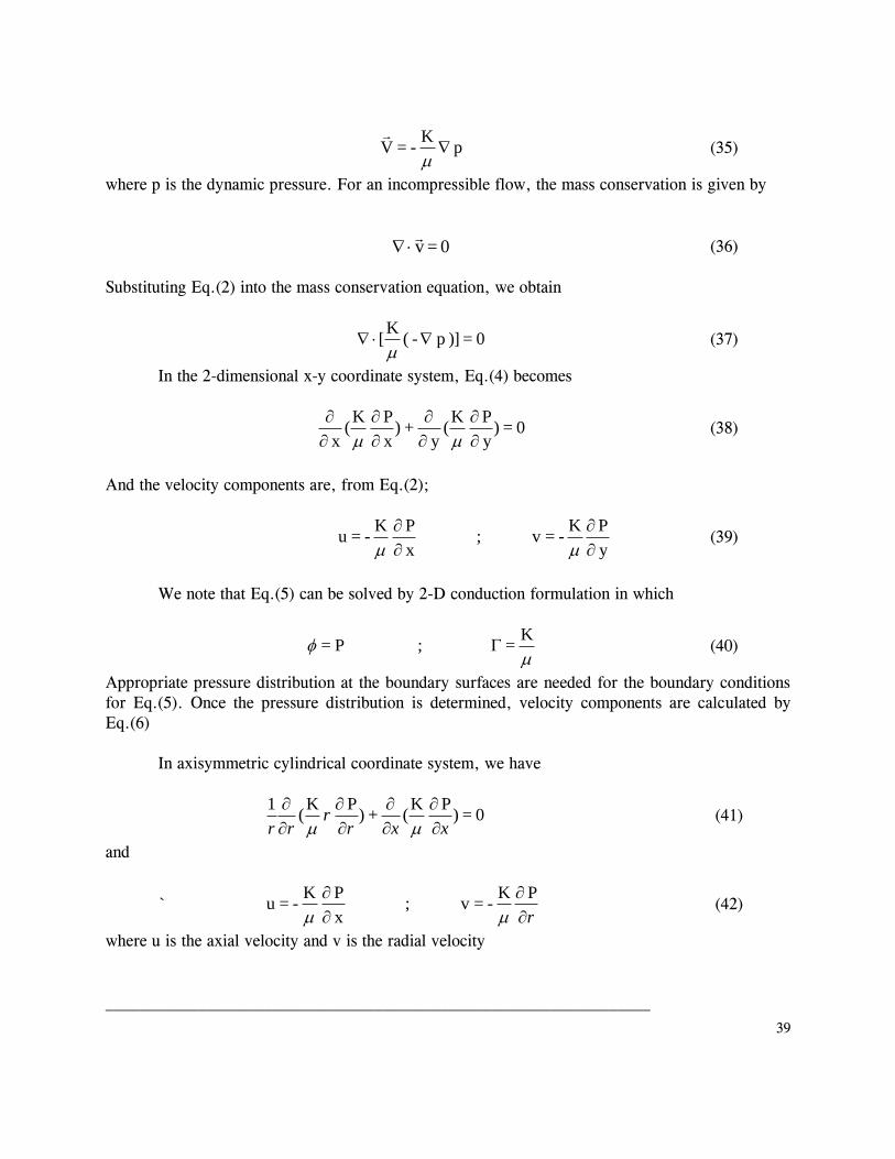
)g + p - (K

= V

(34)

where K is the permeability of the porous medium, is the dynamic viscosity of the fluid and p is

the thermodynamic pressure, which is the sum of hydrostatic and hydrodynamic pressures. By

canceling the hydrostatic pressure gradient and the body force, Eq.(1) reduces to

temperature contour

x(m)

y(m

)

2 4 6 8

0.5

1

1.5

2

2.5

3

3.5

4

0 2 4 6 8 10-0.5

0

0.5

1

1.5

2

2.5

3

3.5

4

4.5

39

p K

- = V

(35)

where p is the dynamic pressure. For an incompressible flow, the mass conservation is given by

0 = v (36)

Substituting Eq.(2) into the mass conservation equation, we obtain

0 = )] p - (K

[

(37)

In the 2-dimensional x-y coordinate system, Eq.(4) becomes

0 = )y

P

K(

y + )

x

P

K(

x

(38)

And the velocity components are, from Eq.(2);

y

PK- = v ;

x

P

K- =u

(39)

We note that Eq.(5) can be solved by 2-D conduction formulation in which

K

= ; P = (40)

Appropriate pressure distribution at the boundary surfaces are needed for the boundary conditions

for Eq.(5). Once the pressure distribution is determined, velocity components are calculated by

Eq.(6)

In axisymmetric cylindrical coordinate system, we have

0 = )P

K

( + )P

K

(1

xxrr

rr

(41)

and

` r

PK- = v ;

x

P

K- =u

(42)

where u is the axial velocity and v is the radial velocity

_________________________________________________________________

40

Example 7

_________________________________________________________________

As an example, flow through a concentric annular wick in a heat pipe application is

considered. Fig. 14 shows a simplified geometry of heat pipe application. Flow enters from

the right opening at the bottom and leaves through the opening at the bottom in the left side.

Pressures are known at the openings. Fluid is ammonia and the permeability of the medium is

3.1x10-9 m2. The ammonia properties are: density (670 kg/m3), and dynamic viscosity (2.1x10-4

kg/ms). The pressures at the inlet and the exit are p1=176 Pa and p2=88 Pa, respectively.

Dimensions are L1=L3=0.3 m, L2=0.9 m and H=Ro -Ri =0.2-0.1=0.1 m. Except the

openings, all surfaces are solid boundary and no flow boundary conditions are used for the

pressure.

A grid system with 15 by 8 uniform control volumes is used for the cylindrical

geometry (geo=2 in cond2d.m). A steady state solution is desired so a very large time step is

used. The diffusion coefficient in this problem is K/. The boundary conditions for the

dependent variable, P are needed. At the vertical solid walls, u=0 and at the horizontal solid

walls, v=0. This implies zero flux boundary condition at all solid boundaries. At the open

boundary, known pressures are prescribed. After obtaining the pressure distribution, velocity u

and v are calculated by Eq. (8).

Figure 14 Flow through a porous medium

A steady state is obtained after 78 iterations. Fig. 15 shows the pressure contours and

the velocity vectors. Except the regions near the inlet and outlet, pressure distribution is almost

linear along the x-direction and the vertical flow speed (v) becomes negligible.

P1

wick

P2

L1

L2

L3

x

y

H

= Ro

Ri

41

Figure 15 Pressure distribution and velocity vectors

Velocity data are saved as a matlab file, uv_porous, that will be used for heat transfer

calculation discussed later. Total volume flow rate is 1.148e-4 m3/s.

Listing of cond2d_porous.mat %cond2d_input_porous.m %transient, 2-dimensional flow in porous medium %Finite volume formulation %%%%%%%%%%%%%%%%%%%%%%%%%%%%%%%%%%%%%%%%%%%%%%%%%%%%%%%%%%%%%%%% % figure2d_convp % geometry selection:geo=1(cartesian, x,y), geo=2(cylindrical axisymmetric,

x=z,y=r), % geo=3 (polar ,x=r,y=theta (in radian)) %in this application dependent variable 'te' is the dynamic pressure %select the geometry close all clear all clc geo=2; %specify the number of control volumes n=15;%number of control volumes in x-direction m=8;%number of control volumes in y-direction np1=n+1; np2=n+2; np3=n+3; mp1=m+1; mp2=m+2; mp3=m+3; maxiter=2000;%maximum iteration number %assign time step and maximum time tstop=100; %time to stop calculation dt=1.0e20; %time increment, dt=1.0e10 for steady state calculation mwrite=0; %time iteration to print the results. If dt>tstop set mwrite=0 re=1;%relaxation coefficient

temperature contour

x(m)

y(m

)

0 0.5 1 1.50.1

0.12

0.14

0.16

0.18

0.2

42

iperiodic=0; jperiodic=0; %define calculation domain width=1.5;% in x-direction delx=width/n; dx=ones(1,np2); dx=delx*dx; if iperiodic==0 dx(1,1)=1.0e-10; dx(1,np2)=1.0e-10; else dx(1)=dx(np1); dx(np2)=dx(2); end % if geo=3 , y is angular direction and must be in radian ro=0.2;%outer radius ri=0.1;%inner radius height=ro-ri;% in y-direction dely=height/m; dy=ones(mp2,1); dy=dely*dy; if jperiodic==0 dy(1,1)=1.0e-10; dy(mp2,1)=1.0e-10; else dy(1)=dy(mp1); dy(mp2)=dy(2); end % %assign x-coordinate if geo==3 x(1,1)=ri;%inner radius for the polar coordinate else x(1,1)=0;%cartesian coordinate or axisymmetric end for i=1:np2 x(1,i+1)=x(1,i)+dx(1,i); end %assign y-coordinate if geo==1 y(1,1)=0;%cartesian coordinate or polar else y(1,1)=ri; %inner radius for axisymmetric end for j=1:mp2 y(j+1,1)=y(j,1)+dy(j,1); end %prescribe intitial values %te=dynamic pressure in this program for j=1:mp2 for i=1:np2 te0(j,i)=0.5*(176+88); te(j,i)=te0(j,i); tep(j,i)=te(j,i); %predicted value at the next iteration end

43

end %%%%%%%%%%%%%%% %time loop begins here t=0;%starting time %plottime=[t]; %plotte=[te(mp2,np2)]; %save data for plot iwrite=1;%printout counter, iwrtie<mwrite means skip print out while t<tstop % calculation continues until t>tstop%%%%%%%%%%%%%%%OUTER LOOP %iteration for convergence in each time step iter=0; iflag=1; %iflag=1 means convergence is not met %iteration loop for the convergence while iflag==1 % end is at the end of program ***************INNER LOOP %prescribe properties pk=3.1e-9;%permeability vis=2.1e-4;%viscocity for i=1:np2 for j=1:mp2 tk(j,i)=pk/vis;%diffusion coefficient ro(j,i)=670;%density cp(j,i)=4740;%specific heat end end %prescribe boundary conditions %initialize fluxes qx0c=zeros(mp2,1); qx0p=zeros(mp2,1); qx0=zeros(mp2,1); qx1c=zeros(mp2,1); qx1p=zeros(mp2,1); qx1=zeros(mp2,1); qy0c=zeros(1,np2); qy0p=zeros(1,np2); qy0=zeros(1,np2); qy1c=zeros(1,np2); qy1p=zeros(1,np2); qy1=zeros(1,np2); %bx0(j)=1,2,3(known temperature, known flux, periodic) at x=0 %bx1(j)=1,2,3 (same) at x=xmax %by0(i)=1,2,3(known temperature, known flux, periodic) at y=0 %by1(i)=1,2,3 (same) at y=ymax %at x=0 & x=xmax for j=1:mp2 bx0(j)=2; bx1(j)=2; end %at y=r1, inner radius for i=1:4 by0(i)=1; te(1,i)=88; end for i=5:13 by0(i)=2; end for i=14:np2

44

by0(i)=1; te(1,i)=2*88; end %y=ro, outer radius for i=1:np2 by1(i)=2; end %evaluate sourec terms for i=1:np2 for j=1:mp2 sp(j,i)=0; sc(j,i)=0; end end %%%%%%%%%%%%%%% cond2d_invariant; %%%%%%%%%%%%%%% end % this end goes with the while iflag==1 at the top************INNER LOOP %solution converged within time step or iter > maxiter %advance to the next time level t=t+dt; %increase time %reinitialize dependent variable for i=1:np2 for j=1:mp2 te0(j,i)=te(j,i);%new temperature becomes old temperature tep(j,i)=te0(j,i); end end %write the results at this time? if iwrite>mwrite %print the results fprintf('iteration number is %i \n',iter) fprintf('time is %9.3f\n',t) iwrite=0; end iwrite=iwrite+1; %plottime=[plottime t]; %plotte=[plotte te(mp2,np2)]; end %this end goes with while t<tstop%%%%%%%%%%%%%%%%%%%%%%%%%%%%%%OUTER LOOP %calculate the velocity using pressure u=zeros(mp2,np3); v=zeros(np2,mp3); %x-direction velocity for j=1:mp2 u(j,1)=0; %solid wall at x=0 u(j,np3)=0;%solid wall at x=L end for i=2:np2 for j=1:mp2 u(j,i)=-tk(j,i)*(te(j,i)-te(j,i-1))/(0.5*(dx(1,i-1)+dx(1,i))); end end %y-direction velocity for i=1:np2 v(mp3,i)=0; %solid wall outer radius

45

v(1,i)=0; %solid wall inner radius end for j=2:mp2 for i=1:np2 v(j,i)=-tk(j,i)*(te(j,i)-te(j-1,i))/(0.5*(dy(j-1,1)+dy(j,1))); end end %open boundary at the inner boundary for i=1:np2 if i<5 | i>13 v(1,i)=v(2,i); end end %save the velocity data save uv_porous u v %plot figure2d_convp(geo,x,y,m,n,te,u,v); %calculate the volume flow rate vdot=0; for i=14:np2 vdot=vdot+v(1,i)*dx(i)*2*pi*y(1); end disp(['volume flow rate m^3/s = ' num2str(vdot)])

46

Problems

1. To improve the heat transfer rate, fins are frequently used. The following diagram shows

fins internally placed in a circular pipe. Internal fins increase heat transfer rate and

pressure drop along the pipe resulting in increased pumping power. Assume same

geometry, flow properties and pressure drop as in Example 7.2, except the presence of

internal fins. Assume a high conductivity wall.

Part 1.

(a) Obtain hydrodynamically fully-developed flow with internal fins. Plot w(x,y)/wavg.

(b) Calculate friction factor times Reynolds number. Use two types of hydraulic diameter;

Dh=D and Dh=4A/wetted perimeter.

Part 2.

(c) Obtain thermally-fully-developed temperature field with internal fins and plot non-

dimensional temperature. Assume axially uniform wall heat flux and high conductivity

wall.

(d) Calculate local Nusselt Number at the surface of the pipe and average Nusselt

number. Use two different types of Dh as in question (b).

47

2. The following diagram shows a cross-section of a heat exchanger with rectangular fins

attached to the base plate. Air is flowing in the z-direction and is fully developed lamanar

flow. The pressure drop in the z-direction is 0.2 pa/m. Use air properties at 300 K and

1 atm pressure.

Part 1:

(a) Determine the fully-developed velocity. Use 2 control volumes for the half thickness

of the fin that falls in the calculation domain, 8 equal control volumes in the

remaining x-distance. Use 8 equal control volumes for the fin height and 4 control

volumes for the clearance.

(b) Plot nondimensional velocity distribution (w/wavg).

(c) Calculate f times Re.

Part 2:

(d) Obtain thermally fully-developed temperature distribution when the top plate is

insulated and the base plate is sujected to a uniform heat flux. Assume conductivity of the

fin is 4 times higher than the conductivity of the fluid.

(e) Plot nondimensional temperature distribution.

(f) Claculate local Nusselt number along the base plate and the average Nusslet

number.

48

3. Consider a fully-developed laminar channel flow as shown in the figure. Three surfaces

are insulated and the top surface is subject to (a) constant heat flux and (b) constant

temperature. Calculate the Nusselt number along the surfaces and the average Nusselt

number. Neglect the presence of the walls.

4. Show that for fully-developed laminar flow through a circular pipe, the average Nusselt

number is 3.66 with constant temperature and 4.36 with constant wall heat flux boundary

conditions.

49

5. Consider a half cylindrical pipe as shown in the figure. The bottom surface is insulated

and the remaining surface is subject to (a) constant wall temperature and (b) constant wall

heat flux. The flow is a fully developed laminar flow.

Calculate (a) the friction factor times the Reynolds number and (b) local and average

Nusselt number for both thermal boundary conditions. Neglect the wall effects.

6. A circular pipe carries a fully-developed laminar flow . The bottom half of the pipe is

insulated and the top half of the pipe is subject to a constant heat flux. Calculate the

local and average Nusselt number.

50

7. A double pipe heat exchanger made of two concentric circular pipes is frequently used. To

improve the heat transfer rate, radial fins are attached thereby increasing the heat transfer area.

Figure shows such a design. In the inner pipe, water vapor at 1 atm pressure is condensing and

the air flows through the sectored annular spaces. Temperature at the inner surface is equal to the

saturation temperature of water vapor at 1 atm (100 0C). Temperature at the fin can be assumed to

be 100 0C since the conductivity of the fin is very large. Outer surface of the pipe is insulated.

Neglect the thickness of the pipes and the fins. Use the same geometry, air flow properties and

pressure drop as in Example 7.2 except the inner pipe (Rin/Rout =0.2) and internal fins.

(a) Obtain hydrodynamically fully-developed velocity distribution using 10 (radial) by 5 (angular)

uniform control volumes. Print and plot w/wavg.

(b) Calculate fRe.

(c) Obtain and plot nondimensional thermally fully-developed temperature distrribution.

(d) Calculate local Nusselt number along the inner surface and along the fin and average Nusselt

number.

(e) Repeat the calculations without internal fins and compare with the results with internal fins in

terms of friction factor and average Nusselt number.

51

8. To improve the heat transfer rate a fin (partition) is placed in the middle of a rectangular

channel as shown in the figure. The aspect ratio, W/H, is 2.0. Assume laminar flow.

Part 1. Hydrodynamically fully developed flow.

(a) By modifying C7E1INP file, obtain hydrodynamically fully developed velocity

distribution, w(x,y). Plot non-dimensional velocity contour w(x,y)/wavg.

(b) Calculate the friction factor times the Reynolds number. Use the same hydraulic diameter

as defined for the channel without the partition. In this way we can compare the effect of

the partition on the friction factor and the pressure drop.

Part 2. Thermally fully developed flow.

(c) Use the velocity distribution obtained in part 1 for a thermally fully developed flow with

constant wall heat flux. Assume a very large conductivity for the walls and the partition.

This implies temperature is uniform in the partition as well as in the walls. Modify

C7E3INP file to include the partition. Plot the non-dimensional temperature distribution.

(d) Calculate the average Nusselt number including the partition. Compare with the case

without the partition.

(e) Discuss the effects of partition on the pressure drop and the rate of heat transfer.

W

H

W/2

H/2

Qw

52

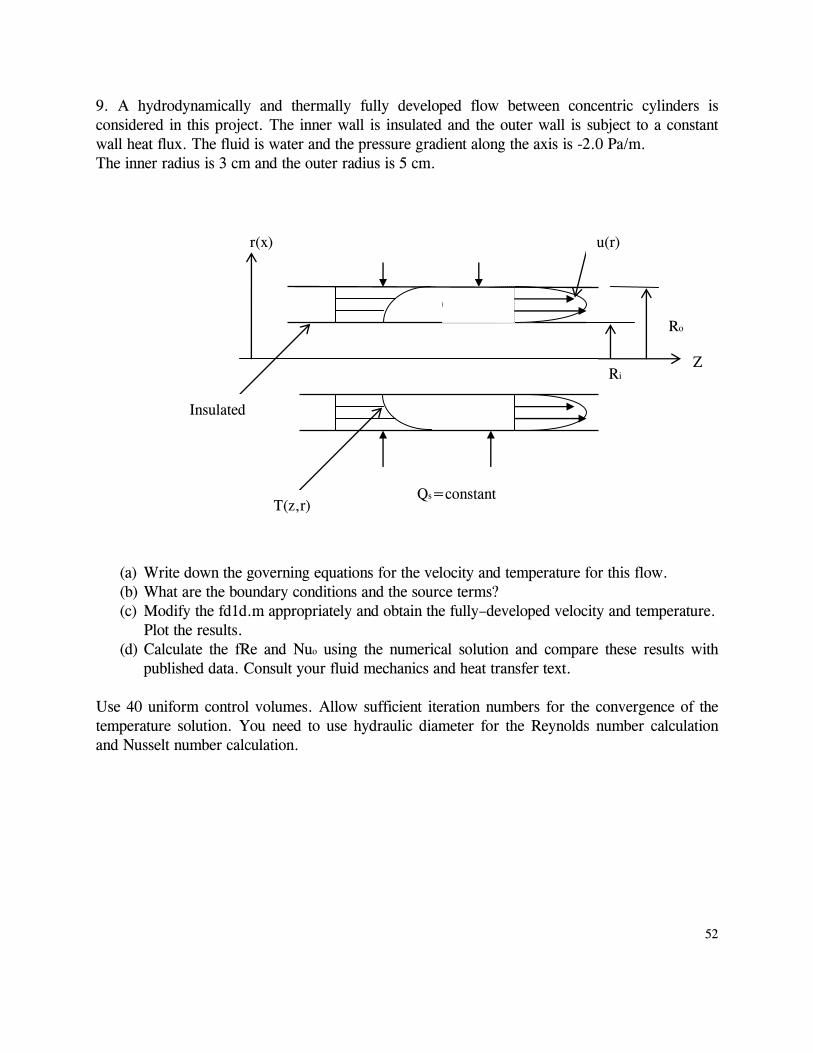
9. A hydrodynamically and thermally fully developed flow between concentric cylinders is

considered in this project. The inner wall is insulated and the outer wall is subject to a constant

wall heat flux. The fluid is water and the pressure gradient along the axis is -2.0 Pa/m.

The inner radius is 3 cm and the outer radius is 5 cm.

(a) Write down the governing equations for the velocity and temperature for this flow.

(b) What are the boundary conditions and the source terms?

(c) Modify the fd1d.m appropriately and obtain the fully–developed velocity and temperature.

Plot the results.

(d) Calculate the fRe and Nuo using the numerical solution and compare these results with

published data. Consult your fluid mechanics and heat transfer text.

Use 40 uniform control volumes. Allow sufficient iteration numbers for the convergence of the

temperature solution. You need to use hydraulic diameter for the Reynolds number calculation

and Nusselt number calculation.

Ro

Ri

Qs=constant T(z,r)

Z

r(x) u(r)

Insulated