conduction and convection phenomena through a … · conduction and convection phenomena through a...

Applied Mathematical Modelling 31 (2007) 1444–1459

www.elsevier.com/locate/apm

Conduction and convection phenomena through a slabwith thermal heterogeneities

A. Tadeu *, N. Simoes

Department of Civil Engineering, Faculty of Sciences and Technology, University of Coimbra, Polo II,

Pinhal de Marrocos, 3030-290 Coimbra, Portugal

Received 1 June 2005; received in revised form 1 November 2005; accepted 12 April 2006Available online 30 June 2006

Abstract

This paper addresses the computation of the three-dimensional transient heat transfer through a layered solid and/orfluid formation containing irregular inclusions. The use of appropriate Green’s functions for a flat layer formation in aboundary element method formulation avoids the discretization of the layer interface boundaries.

Both conduction and convection are taken into account in the heat diffusion generated by a source, placed somewherein the layered system, assuming a known convection velocity field. This work is an extension of earlier work by the authors,in which only the conduction phenomenon was considered. As before, the calculation process is defined first in thefrequency domain, while the final time series are later computed by applying inverse (fast) Fourier transforms. Onceagain, complex frequencies are used in order to avoid aliasing phenomena.

The applicability of the model is illustrated by solving the case of a solid layer submerged in a fluid medium andcontaining multiple circular cylindrical thermal heterogeneities. The importance of convection phenomena is studied fordifferent inclusions’ thermal properties.� 2006 Elsevier Inc. All rights reserved.

Keywords: Transient heat transfer; Conduction; Convection; Boundary element method; 2.5D Green’s functions; Frequency domain;Fourier transform

1. Introduction

Analytical solutions can only be used to solve simple problems, while the boundary element method (BEM)can be applied to deal with general problems. The BEM provides an alternative to the well established finiteelement method (FEM) for solving physical problems, such as that of heat diffusion, for which BEM codeshave been developed by various authors, including Brebbia et al. [1], Pina and Fernandez [2]. Most of theknown techniques that use BEM to solve transient heat transfer problems utilize ‘‘time marching schemes’’or Laplace transforms.

0307-904X/$ - see front matter � 2006 Elsevier Inc. All rights reserved.

doi:10.1016/j.apm.2006.04.010

* Corresponding author. Tel.: +351 239797204; fax: +351 239797190.E-mail address: [email protected] (A. Tadeu).

mailto:[email protected]

A. Tadeu, N. Simoes / Applied Mathematical Modelling 31 (2007) 1444–1459 1445

As examples of ‘‘time marching’’ approaches, several works can be cited: Chang et al. [3] and Shaw [4] useda time-dependent fundamental solution for studying transient heat processes; later, Wrobel and Brebbia [5]described a formulation for axisymmetric diffusion problems; Carini et al. [6] implemented a symmetricboundary element method for studying the transient heat conduction over a two-dimensional homogeneousdomain using semi-analytical integrations; also using a time marching boundary element method, Lesnicet al. [7] solved the unsteady diffusion equation in both one and two dimensions, taking into account the treat-ment of singularities.

As mentioned above, an alternative numerical scheme, the Laplace transform technique, can be imple-mented, too, to solve heat transfer problems. The purpose is to remove the time-dependent derivative, usinginstead a transform variable. However, this process then requires an inverse transform to find the solutionin the time domain. A Laplace transform boundary element method approach was used, for example, bySutradhar et al. [8,9] to solve the three-dimensional transient heat conduction in functionally gradedmaterials.

Several numerical schemes have been proposed to improve the efficiency of the BEM and its applicability tomore general problems, such as those involving nonlinearities. The dual reciprocity boundary method(DRBEM) is one of these techniques, and this was originally proposed by Nardini and Brebbia [10]. A numberof works were subsequently published, including those by Satravaha and Zhu [11,12], applying the Laplacetransform dual reciprocity method to the case of transient heat conduction in the presence of nonlinear mate-rial properties (thermal conductivity, density and specific heat coefficients were all assumed to be functions oftemperature), boundary conditions and sources. Guven and Madenci [13] developed a coupled finite element–boundary element analysis method for the solution of transient two-dimensional heat conduction of domainswith dissimilar materials and geometric discontinuities. Tanaka and Tanaka [14] studied the heat conductionin anisotropic non-homogeneous media using a BEM formulation based on the application of fundamentalsolutions for a fictitious homogeneous medium. This approach was first used by Butterfield for potential flowproblems [15]. In order to study the transient heat conduction with nonlinear source terms in a domain wherethe thermal material properties change in spatial co-ordinates Sladek et al. [16] applied a local boundary inte-gral equation method.

The BEM requires the discretization of the solid and fluid thermal interfaces and the knowledge of funda-mental solutions. The definition of suitable Green’s functions can avoid the discretization of some of thosethermal interfaces, leading to a more efficient formulation. This paper computes the three-dimensional tran-sient heat transfer through a flat-layered formation that contains heterogeneities, using Green’s functions thatavoid the discretization of the flat interfaces.

The technique proposed in this paper is an adaptation and extension of a formulation used by the authorsto solve a similar problem, where only the conduction phenomenon was addressed [17]. In the work describedhere, both the conduction and the convection phenomena are taken into account with a pre-prescribed con-vection velocity.

The technique proposed makes use of time Fourier transforms to allow the calculations to be made in thefrequency domain. This procedure overcomes some of the difficulties posed by the ‘‘time marching’’ andLaplace transforms approach, which may lead to loss of accuracy and the amplification of small truncationerrors. If a spatial Fourier transform is then applied in the z and x directions the three-dimensional solutioncan be obtained as a sum of 2D problems with different spatial wavenumbers kz and kx.

The Green’s functions for a layered medium, without heterogeneities, can be obtained as a superposition ofheat plane sources, as was described originally by Lamb [18] for the propagation of elastodynamic waves intwo-dimensional media. This approach was later adopted by other authors, such as Bouchon [19] and Tadeuand Antonio [20] to compute three-dimensional elastodynamic fields using a discrete wave number represen-tation. The solution can be expressed as the sum of the heat source terms equal to those in the unboundedspace and the surface terms. These last terms need to satisfy the boundary conditions at the flat layer inter-faces: continuity of normal fluxes and temperatures.

This paper first defines the three-dimensional problem and describes how the solution for a point source,applied in an infinite domain, can be written as a continuous superposition of heat plane terms, in the fre-quency domain. The time domain solutions, obtained after applying inverse frequency and spatial Fouriertransforms, are compared with analytical solutions [21,22]. Next, the analytical Green’s functions for a layer

1446 A. Tadeu, N. Simoes / Applied Mathematical Modelling 31 (2007) 1444–1459

formation bounded by two semi-infinite media are described, implemented and compared with those com-puted by the BEM model, which incorporates Green’s functions for an unbounded medium and have the dis-advantage of requiring the discretization of the boundary interfaces. Notice that the extension of theinterfaces’ discretization is limited by introducing damping; otherwise the system of equations involved wouldbe too large to be solved.

These Green’s functions are then incorporated into a BEM code to compute the heat transfer in the pres-ence of cylindrical thermal heterogeneities placed in a solid layer bounded by two semi-infinite layers. Differentsimulations are performed to illustrate the applicability of the proposed model, and to evaluate the importanceof the convection phenomena and the presence of thermal heterogeneities in heat diffusion across a solid layerbounded by fluid media.

2. 3D problem formulation

Transient heat transfer by conduction and convection in a homogeneous, isotropic body can be modelledby

o2

ox2þ o2

oy2þ o2

oz2

� �T � 1

KV x

o

oxþ V y

o

oyþ V z

o

oz

� �T ¼ 1

KoTot; ð1Þ

in which Vx, Vy and Vz are the pre-prescribed velocity components in directions x, y and z respectively, t istime, T(t,x,y,z) is temperature, K = k/(qc) is the thermal diffusivity, k is the thermal conductivity, q is the den-sity and c is the specific heat. A Fourier transformation in the time domain applied to Eq. (1) gives the equa-tion below, expressed in the frequency domain

o2

ox2þ o

2

oy2þ o

2

oz2

� �� 1

KV x

o

oxþ V y

o

oyþ V z

o

oz

� �þ

ffiffiffiffiffiffiffiffiffi�ix

K

r !20@ 1AbT ðx; x; y; zÞ ¼ 0; ð2Þ

where i ¼ffiffiffiffiffiffiffi�1p

and x is the frequency. Eq. (2) differs from the Helmholtz equation by the presence of a con-vective term. For a heat point source, applied at (0,0,0) in an unbounded medium, of the formp(x,x,y,z, t) = d(x)d(y)d(z)ei(xt), where d(y) and d(z) are Dirac-delta functions, the fundamental solution ofEq. (2) (see [22]) can be expressed as

bT f ðx; x; y; zÞ ¼e

V xxþV y yþV zz2K

2kffiffiffiffiffiffiffiffiffiffiffiffiffiffiffiffiffiffiffiffiffiffiffiffix2 þ y2 þ z2

p e�i

ffiffiffiffiffiffiffiffiffiffiffiffiffiffiffiffiffiffiffiffiffi�

V 2xþV 2

yþV 2z

4K2 �ixK

q ffiffiffiffiffiffiffiffiffiffiffiffiffiffix2þy2þz2p

: ð3Þ

To avoid the computational requirements of 3D problem formulation when the geometry of the problem re-mains constant along the z direction, the full 3D problem can be expressed as a summation of simpler 2D solu-tions. This requires the application of a Fourier transformation along that direction, writing this as asummation of 2D solutions with different spatial wavenumbers kz (see [23]). The application of a spatial Fou-rier transformation to

e�i

ffiffiffiffiffiffiffiffiffiffiffiffiffiffiffiffiffiffiffiffiffi�

V 2xþV 2

yþV 2z

4K2 �ixK

q ffiffiffiffiffiffiffiffiffiffiffiffiffiffix2þy2þz2p

ffiffiffiffiffiffiffiffiffiffiffiffiffiffiffiffiffiffiffiffiffiffiffiffix2 þ y2 þ z2

p ; ð4Þ

along the z direction, leads to this fundamental solution

eT f ðx; x; y; kzÞ ¼�ie

V xxþV y yþV zz2K

4kH0

ffiffiffiffiffiffiffiffiffiffiffiffiffiffiffiffiffiffiffiffiffiffiffiffiffiffiffiffiffiffiffiffiffiffiffiffiffiffiffiffiffiffiffiffiffiffiffiffiffiffiffiffiffiffiffiffiffiffi�

V 2x þ V 2

y þ V 2z

4K2� ix

K� ðkzÞ2

sr0

0@ 1A; ð5Þ

where H0( ) are Hankel functions of the second kind and order 0, and r0 ¼ffiffiffiffiffiffiffiffiffiffiffiffiffiffix2 þ y2

p.

This response is related to a spatially varying heat line source of the type pðx; x; y; kz; tÞ ¼ dðxÞdðyÞeiðxt�kzzÞ

(see Fig. 1).

x

y

z

(0,0 ,0)

Fig. 1. Spatially harmonic varying line load.


The full three-dimensional solution can be synthesized by applying an inverse Fourier transform along the

kz domain to the expression �i2

H0

ffiffiffiffiffiffiffiffiffiffiffiffiffiffiffiffiffiffiffiffiffiffiffiffiffiffiffiffiffiffiffiffiffiffiffiffiffiffiffiffiffiffiffiffiffi� V 2

xþV 2yþV 2

z

4K2 � ixK � ðkzÞ2

qr0

� �,

eT ðx; x; y; zÞ ¼ eV xxþV y yþV zz

2K


p Z 1

�1

�i

2H0

ffiffiffiffiffiffiffiffiffiffiffiffiffiffiffiffiffiffiffiffiffiffiffiffiffiffiffiffiffiffiffiffiffiffiffiffiffiffiffiffiffiffiffiffiffiffiffiffiffiffiffiffiffiffiffiffiffiffi�

V 2x þ V 2

y þ V 2z

4K2� ix

K� ðkzÞ2

sr0

0@ 1Ae�ikzz dkz: ð6Þ

Assuming the existence of virtual sources, equally spaced at Lz, along z, then Eq. (6) changes into

eT ðx; x; y; zÞ ¼ eV xxþV y yþV zz

2K

2kffiffiffiffiffiffiffiffiffiffiffiffiffiffiffiffiffiffiffiffiffiffiffix2 þ y2 þ z2

p Z 1

�1

�i

2H0

ffiffiffiffiffiffiffiffiffiffiffiffiffiffiffiffiffiffiffiffiffiffiffiffiffiffiffiffiffiffiffiffiffiffiffiffiffiffiffiffiffiffiffiffiffiffiffiffiffiffiffiffiffiffiffiffiffi�

V 2x þ V 2

y þ V 2z

4K2� ix

K� ðkzÞ2

sr0

0@ 1Ae�ikzzX1

m¼�1e�ikzmLz dkz: ð7Þ

Using the results from distribution theory (e.g. [24]) this equation can be expressed as

eT ðx; x; y; zÞ ¼ 2pLz

eV xxþV y yþV zz

2K


p X1m¼�1

H0

ffiffiffiffiffiffiffiffiffiffiffiffiffiffiffiffiffiffiffiffiffiffiffiffiffiffiffiffiffiffiffiffiffiffiffiffiffiffiffiffiffiffiffiffiffiffiffiffiffiffiffiffiffiffiffiffiffiffiffiffi�

V 2x þ V 2

y þ V 2z

4K2� ix

K� ðkzmÞ2

sr0

0@ 1Ae�ikzmz; ð8Þ

where kzm is the axial wavenumber given by kzm ¼ 2pLz

m. Eq. (8) can be approximated in turn by a finite discretesummation, which enables the solution to be obtained by solving a limited number of two-dimensionalproblems,

eT ðx; x; y; zÞ ¼ 2pLz

eV xxþV y yþV zz

2K


p XM

m¼�M

H0

ffiffiffiffiffiffiffiffiffiffiffiffiffiffiffiffiffiffiffiffiffiffiffiffiffiffiffiffiffiffiffiffiffiffiffiffiffiffiffiffiffiffiffiffiffiffiffiffiffiffiffiffiffiffiffiffiffiffiffiffi�

V 2x þ V 2

y þ V 2z

4K2� ix

K� ðkzmÞ2

sr0

0@ 1Ae�ikzmz: ð9Þ

The distance Lz must be large enough to prevent spatial contamination from the virtual sources [25]. An anal-ogous approach has been used by Tadeu et al. [26] and Godinho et al. [27] to solve problems of wavepropagation.

The fundamental solution of the differential equation obtained from Eq. (2) after the application of a spa-tial Fourier transformation along the z direction (see Eq. (10)) is Eq. (5), with Vz = 0.

o2

ox2þ o2

oy2

� �� 1

KV x

o

oxþ V y

o

oy

� �þ

ffiffiffiffiffiffiffiffiffiffiffiffiffiffiffiffiffiffiffiffiffiffiffiffi�ix

K� ðkzÞ2

r !20@ 1AeT ðx; x; y; kzÞ ¼ 0: ð10Þ

Eq. (5), for a spatially sinusoidal harmonic heat line source applied at the point (0, 0) along the z direction,subject to convection velocities Vx, Vy and Vz, can be further manipulated and written as a continuous super-position of heat plane phenomena, as in Garvin [28],


V xxþV y yþV zz2K

4pk

Z þ1

�1

e�imjyj

m

� �e�ikxðxÞ dkx; ð11Þ


where m ¼ffiffiffiffiffiffiffiffiffiffiffiffiffiffiffiffiffiffiffiffiffiffiffiffiffiffiffiffiffiffiffiffiffiffiffiffiffiffiffiffiffiffiffiffiffiffiffiffiffiffiffiffiffiffiffi� V 2

xþV 2yþV 2

z

2K � ixK � ðkzÞ2 � k2

x

qwith (Im(m) 6 0), and the integration is related to the horizontal wave

number (kx) along the x direction. The use of the expansion of the Hankel function is described by Morse andFeshbach [29].

Assuming the existence of an infinite number of virtual sources, these continuous integrals can be trans-formed into a summation if an infinite number of such sources is distributed along the x direction, spacedat equal intervals Lx. The above equation can then be written as


V xxþV y yþV zz2K

4kE0

Xn¼þ1n¼�1

Emn

� �Ed; ð12Þ

where E0 ¼ �i2kLx

, E ¼ e�imnjyj, Ed ¼ e�ikxnðxÞ, mn ¼ffiffiffiffiffiffiffiffiffiffiffiffiffiffiffiffiffiffiffiffiffiffiffiffiffiffiffiffiffiffiffiffiffiffiffiffiffiffiffiffiffiffiffiffiffiffiffiffiffiffiffiffiffiffiffiffi� V 2

xþV 2yþV 2

z

4K2 � ixK � ðkzÞ2 � k2

xn

qwith (Im(mn) 6 0), kxn ¼ 2p

Lxn,

which can in turn be approximated by a finite sum of equations (N). Note that kz = 0 corresponds to thetwo-dimensional case.

2.1. Responses in the time domain

The heat responses in the spatial–temporal domain are obtained by means of an inverse fast Fourier trans-form in kz and kx and in the frequency domain. In order to prevent the aliasing phenomena, complex frequen-cies with a small imaginary part of the form xc = x � ig (with g = 0.7Dx, and Dx being the frequency step)are used in the computation procedure. The constant g cannot be made arbitrarily large, since this leads eitherto severe loss of numerical precision, or to underflows and overflows in the evaluation of the exponential win-dows (see [30]). The time evolution of the heat source amplitude can be diversified. The time Fourier transfor-mation of the incident heat field defines the frequency domain where the BEM solution needs to be computed.The response may need to be computed from 0.0 Hz up to very high frequencies. An intrinsic characteristic ofthis problem is that the heat responses decay very fast as the frequency increases, which allows us to limit theupper frequency for the solution. The static response can be computed when the frequency is zero, since theuse of complex frequencies leads to arguments for the Hankel function that are different from zero (xc = �igfor 0.0 Hz).

2.2. Verification of the solution

The formulation described above was verified by computing heat propagation in an unbounded mediumwhen conduction and convection are considered. The results obtained were compared with the analyticalresponse in the time domain.

The exact solution of the three, two or one-dimensional convective diffusion, expressed by Eq. (1), in anunbounded medium subjected to a unit heat source can be found in the literature, see Banerjee [21]. The timesolution at (x,y,z) for a unit heat source placed at (0,0,0) at time t = t0 in an unbounded medium is given bythe expression

T ðt; x; y; zÞ ¼ e�ð�sV xþxÞ2�ð�sV yþyÞ2�ð�sV zþzÞ2

4Ks

qcð4pKsÞd=2; if t > t0; ð13Þ

where s = t � t0; the parameter d can be 3, 2 or 1 depending on whether we are in the presence of a three, twoor one-dimensional problem, respectively.

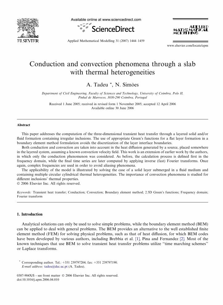
The verification example assumes that a homogeneous unbounded medium was excited by a cylindricalheat source (d = 2) placed at (0,0,0). The material’s density (q), specific heat (c), and the thermal conductivity(k) attributed to the medium were 2300 kg m�3, 880.0 J kg�1 �C�1 and 1.4 W m�1 �C�1, respectively. The con-vection velocity ascribed in the x, y directions was 1 · 10�6 m/s.

The heat responses were calculated along a line of 40 receivers placed from (x = �1.5, y = 0.35, z = 0) to(x = 1.5, y = 0.35, z = 0). The calculations, using the formulation described above, were done in the frequencyrange [0, 1024 · 10�7 Hz] with an increment of Dx = 10�7 Hz, which defines a time window of T = 2777.8 h.

0

0.1

0.2

0.3

0.4

0.5

-1.5 -1.0 -0.5 0 0.5 1.0 1.5

350 h450 h550 h650 h

X (m)

Tem

per

atu

re (

°C)

Fig. 2. Temperature distribution along a line of 40 receivers, at different times (350 h, 450 h, 550 h and 650 h) for a cylindrical (d = 2) unitheat source.


The correspondent time domain responses were obtained by applying a numerical inverse fast Fouriertransform in kz and in the frequency domain. These responses are illustrated in Fig. 2 by marks, while the solidlines indicate the solution computed using Eq. (13). The two solutions show good agreement. It is interestingto note that the response is not symmetric because of the convection phenomenon in the x direction.

2.3. 2.5D heat diffusion Green’s functions in a flat layer bounded by two unbounded media

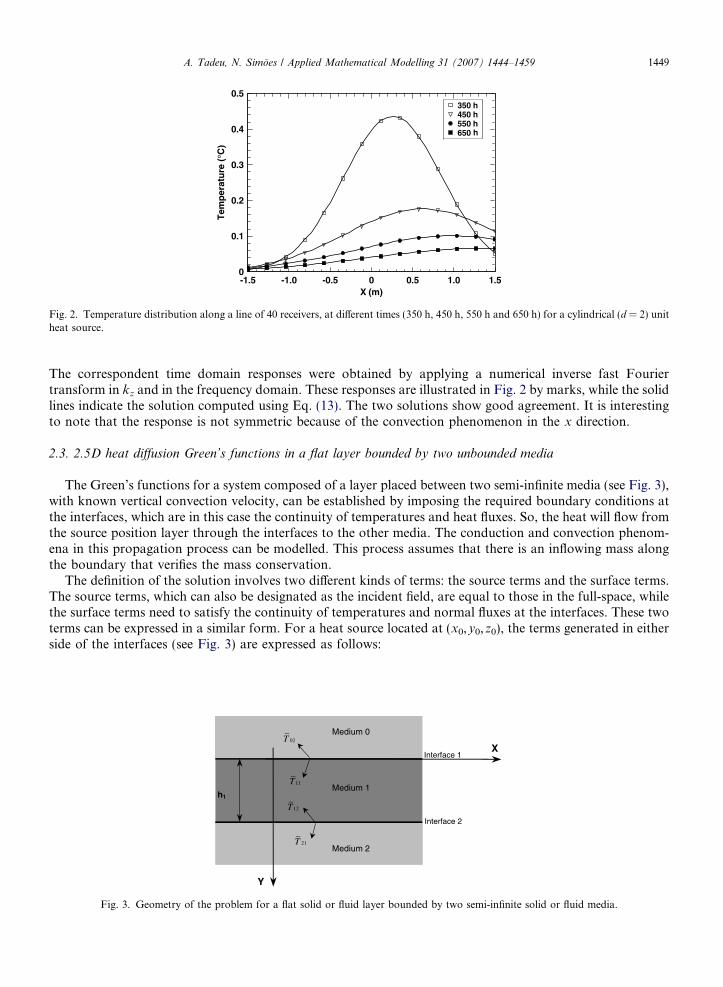
The Green’s functions for a system composed of a layer placed between two semi-infinite media (see Fig. 3),with known vertical convection velocity, can be established by imposing the required boundary conditions atthe interfaces, which are in this case the continuity of temperatures and heat fluxes. So, the heat will flow fromthe source position layer through the interfaces to the other media. The conduction and convection phenom-ena in this propagation process can be modelled. This process assumes that there is an inflowing mass alongthe boundary that verifies the mass conservation.

The definition of the solution involves two different kinds of terms: the source terms and the surface terms.The source terms, which can also be designated as the incident field, are equal to those in the full-space, whilethe surface terms need to satisfy the continuity of temperatures and normal fluxes at the interfaces. These twoterms can be expressed in a similar form. For a heat source located at (x0,y0,z0), the terms generated in eitherside of the interfaces (see Fig. 3) are expressed as follows:

X

Medium 0

Medium 2

h1

Y

Interface 1

Interface 2

Medium 1

~02T

~11T

~12T

~21T

Fig. 3. Geometry of the problem for a flat solid or fluid layer bounded by two semi-infinite solid or fluid media.


Upper semi-infinite space (interface 1)

eT 02ðx; x; y; kzÞ ¼ E00eV y0ðy�y0Þ

2K0

Xn¼þ1n¼�1

E01

mn0

Abn0

� �Ed; ð14Þ

Solid layer (interface 1)


2K1

Xn¼þ1n¼�1

E11

mn1

Atn1

� �Ed; ð15Þ

Solid layer (interface 2)


2K1

Xn¼þ1n¼�1

E12

mn1

Abn1

� �Ed; ð16Þ

Lower semi-infinite space (interface 2)


2K2

Xn¼þ1n¼�1

E21

mn2

Atn2

� �Ed; ð17Þ

where E0j = � i/2kjLx, E00 ¼ e�imn0y , E11 ¼ e�imn1y , E12 ¼ e�imn1jy�h1j, E21 ¼ e�imn2jy�h1j and mnj ¼ffiffiffiffiffiffiffiffiffiffiffiffiffiffiffiffiffiffiffiffiffiffiffiffiffiffiffiffiffiffiffiffiffiffiffiffiffiffiffiffiffiffiffiffiffiffiffiffiffiffiffiffiffiffiffiffiffiffiffiffiffiffiffiffiffi�ðV yj=2KjÞ2 � ix=Kj � k2

z � k2xn

qwith Im(mnj) 6 0 (j = 1 corresponds to the intermediate layer (medium 1),

while j = 0 and j = 2 indicate the upper and lower semi-infinite media, respectively (medium 0, 2)). Meanwhile,Kj = kj/qjcj is the thermal diffusivity in the medium j (kj, qj and cj are the thermal conductivity, the density andthe specific heat of the material in the medium, j, respectively) and Vyj is the convection in the y direction in thefluid medium j.

The unknown coefficients Abn0, At

n1, Abn1 and At

n2 are computed by establishing the appropriate boundary con-ditions, so that the field produced simultaneously by the source and surface terms leads to the continuity ofheat fluxes and temperatures at y = h1 and y = 0. Assuming that the heat source is in the intermediate layer,the following system results when the boundary conditions are imposed for each value of n:

V y0

2K0þ imn0

h ic10

c21� V y1

2K1� imn1

h i� V y1

2K1þ imn1

h ie�imn1h1 0

k1c30

k0c41�1 �e�imn1h1 0

0V y1

2K1� imn1

h ie�imn1h1

V y1

2K1þ imn1

h i� V y2

2K2� imn2

h ic22

c11

0 e�imn1h1 1 � k1c22

k2c11

2666664

3777775Ab

n0

Atn1

Abn1

Atn2

26643775 ¼

b1

b2

b3

b4

26643775; ð18Þ

where c1j ¼ 1mnj

eV yjðPj

l¼1hl�y0Þ

2Kj , c2j ¼ 1mnj

eV yjðPj�1

l¼1hl�y0Þ

2Kj , while b1 ¼ ½V y1=2K1 þ imn1�e�imn1y0 , b2 ¼ e�imn1y0 , b3 ¼�½V y1=2K1 � imn1�e�imn1jh1�y0j and b4 ¼ �e�imn1jh1�y0j, if the source is in the intermediate layer (0 < y0 < h1).

The temperature for the three-layer media is computed by adding the contribution of the source terms tothat associated with the surface terms originated at the various interfaces. This leads to the following expres-sions for the temperatures in the three media, when the source is in the intermediate layer,

eT ðx; x; y; kzÞ ¼ E00eV y0ðy�y0Þ

2K0

Xn¼þ1n¼�1

E01

mn0

Abn0

� �Ed; if y < 0;

eT ðx; x; y; kzÞ ¼�i

4k1

eV y1ðy�y0Þ

2K1 H0ðKt1r1Þ þ E01eV y1ðy�y0Þ

2K1

�Xn¼þ1

n¼�1

E11

mn1

Atn1 þ

E12

mn1

Abn1

� �Ed; if 0 < y < h1;

eT ðx; x; y; kzÞ ¼ E02eV y2ðy�y0Þ

2K2

Xn¼þ1n¼�1

E21

mn2

Atn2

� �Ed; if y > h1;

ð19Þ

where Kt1 ¼ffiffiffiffiffiffiffiffiffiffiffiffiffiffiffiffiffiffiffiffiffiffiffiffiffiffiffiffiffiffiffiffiffiffiffi� V 2

y1

4K21

� ixK1� ðkzÞ2

rand r1 ¼

ffiffiffiffiffiffiffiffiffiffiffiffiffiffiffiffiffiffiffiffiffiffiffiffiffiffiffiffiffiffiffiffiffiffiffiffiffiffiffiffiffiðx� x0Þ2 þ ðy � y0Þ

2q

.


This derivation assumes that the spatially sinusoidal harmonic heat source is located in the intermediatelayer. However, the equations can be easily manipulated to cater for another position of the source.

3. Boundary element formulation

The fundamental BEM equations are not described in detail here, since they can be found in Wrobel [5].The boundary integral equations for a homogeneous isotropic medium layer that is embedded by an infinitemedium and contains a cylindrical body (bounded by a surface S), when this system is subjected to an incidentheat field given by eT inc, are expressed as follows:

along the exterior domain

peT ðextÞðx0; y0; kz;xÞ ¼Z

S

qðextÞðx; y; gn; kz;xÞGðextÞðx; y; x0; y0; kz;xÞds

�Z

S

H ðextÞðx; y; gn; x0; y0; kz;xÞeT ðextÞðx; y; kz;xÞds

�Z

S

GðextÞðx; y; x0; y0; kz;xÞeT ðextÞðx; y; kz;xÞV ðextÞn dsþ eT incðx0; y0; kz;xÞ; ð20Þ

along the interior domain

peT ðintÞðx0; y0; kz;xÞ ¼Z

S

qðintÞðx; y; gn; kz;xÞGðintÞðx; y; x0; y0; kz;xÞds

�Z

S

H ðintÞðx; y; gn; x0; y0; kz;xÞeT ðintÞðx; y; kz;xÞds

�Z

S

GðintÞðx; y; x0; y0; kz;xÞeT ðintÞðx; y; kz;xÞV ðintÞn ds: ð21Þ

The boundary integral equations incorporate a convective term, where Vn = Vxnx + Vyny. In these equations,the superscripts ‘‘int’’ and ‘‘ext’’ refer to the interior and exterior domains respectively, gn is the unit outwardnormal along the boundary, G and H are respectively the fundamental solutions (Green’s functions) for thetemperature (eT Þ and heat flux (q), at (x,y) due to a virtual point heat load at (x0,y0). The factor p is a constantdefined by the shape of the boundary, taking the value 1/2 if the shape is smooth and (x0,y0) 2 S. Note thatthis formulation assumes initial conditions of null temperatures and null heat fluxes throughout the domain.Other initial conditions would require the evaluation of surface or volume integrals.

If the boundary is discretized into N straight boundary elements, with one nodal point in the middle of eachelement, Eqs. (20) and (21) take the form:

along the exterior domain
XN
l¼1

qðextÞklGðextÞkl �XN

l¼1

eT ðextÞklH ðextÞkl �XN

l¼1

GðextÞkleT ðextÞklV ðextÞn þ eT k

incl¼ pkl

eT ðextÞkl; ð22Þ

along the interior domain
XN
l¼1

qðintÞklGðintÞkl �XN

l¼1

eT ðintÞklH ðintÞkl �XN

l¼1

GðintÞkleT ðintÞklVnðintÞ ¼ pkleT ðintÞkl; ð23Þ

where

q(ext)kl and eT ðextÞkl are the nodal heat fluxes and temperatures in the exterior domain,q(int)kl and eT ðintÞkl are the nodal heat fluxes and temperatures in the interior domain,H ðextÞkl ¼

RCl

H ðextÞðx; xl; yl; gl; xk; yk; kzÞdCl; H ðintÞkl ¼R

ClH ðintÞðx; xl; yl; gl; xk; yk; kzÞdCl;

GðextÞkl ¼R

ClGðextÞðx; xl; yl; xk; yk; kzÞdCl; GðintÞkl ¼

RCl

GðintÞðx; xl; yl; xk; yk; kzÞdCl;


where gl is the unit outward normal for the lth boundary segment Cl. In Eqs. (22) and (23), H(ext) (x,xl,yl,gl,xk,yk,kz) and G(ext) (x,xl,yl,xk,yk,kz) are respectively the Green’s functions for the heat fluxes and tempera-ture components in the exterior medium of the inclusion, that is, for a flat layer bounded by two unboundedmedia. H(int)(x,xl,yl,gl,xk,yk,kz) and G(int) (x,xl,yl,xk,yk,kz) are respectively the Green’s functions for theheat fluxes and temperature components in the interior medium of the inclusion, that is, for an unboundedmedium, at point (xl,yl), caused by a concentrated heat load acting at the source point (xk,yk). If the loadedelement coincides with the element being integrated, the factor pkl takes the value 1/2.

The two-and-a-half dimensional Green’s functions for temperature and heat fluxes in Cartesian co-ordi-nates are those for an unbounded medium,

Fig. 4.infinite

Gðx; y; x0; y0; kz;xÞ ¼�i

4ke

Vr02K H0ðktrrÞ;

Hðx; xl; yl; gl; xk; yk; kzÞ ¼�i

4e

Vr02K

V2K

or0

ogl

� �H0ðktrrÞ � ktrH 1ðktrrÞ

orogl

� �� ;

ð24Þ

where V is the assumed radial convection velocity, ktr ¼ffiffiffiffiffiffiffiffiffiffiffiffiffiffiffiffiffiffiffiffiffiffiffiffiffiffiffiffiffiffiffiffiffi�V 2

4K2 þ �ixK � ðkzÞ2

q, r ¼

ffiffiffiffiffiffiffiffiffiffiffiffiffiffiffiffiffiffiffiffiffiffiffiffiffiffiffiffiffiffiffiffiffiffiffiffiffiffiffiffiffiffiffiffiðxl � xkÞ2 þ ðyl � ykÞ

2q

,

r0 ¼ffiffiffiffiffiffiffiffiffiffiffiffiffiffix2 þ y2

pis the distance to the convection source position, and Hn( ) are Hankel functions of the second

kind and order n.If the element to be integrated is not the loaded element, the integrations in Eqs. (22) and (23) are evaluated

using a Gaussian quadrature scheme, while for the loaded element, the existing singular integrands in thesource terms of the Green’s functions are calculated in closed form (see Tadeu et al. [31,32]).

The final system of equations is assembled assuring the continuity of temperatures and heat fluxes along theboundary of the inclusion. The unknown nodal temperatures and heat fluxes are obtained by solving this sys-tem of equations, allowing the heat field along the domain to be defined.

The final integral equations are manipulated and combined so as to impose the continuity of temperaturesand heat fluxes along the boundary of the inclusion, and a system of equations is assembled. The solution ofthis system of equations gives the nodal temperatures and heat fluxes, which allow the reflected heat field to bedefined.

4. Verification of the Green’s functions

In order to verify the accuracy of the Green’s functions, the results were compared with those arrived byapplying the BEM model using the Green’s solutions for an unbounded medium. BEM applications imply thediscretization of all material interfaces. Notice that the BEM code implemented and used here was first testedusing a simple problem geometry (circular cylindrical geometries), for which analytical solutions are known(not included here).

XMedium 1

Medium 1

h1=0.50 m

Y

• SourceRec. 1

Interface 1

Interface 2

Rec. 3

Medium 2 Rec. 2

Geometry of the problem used in the verification of the Green’s functions. A 0.5 m thick layer (medium 2), bounded by two semi-media (media 1).

Table 1Material’s thermal properties used for the verification of the Green’s functions

Medium 1 Medium 2

Thermal conductivity, k [W m�1 �C�1] 0.72 1.4Density, q [kg m�3] 1860.0 2300.0Specific heat, cp [J kg�1 �C�1] 780.0 880.0


The performance of the analytical Green’s functions is illustrated using a system built by a layer (medium2), 0.5 m thick, placed between two unbounded media (media 1), as shown in Fig. 4. A harmonic heat linesource is applied in medium 2 at point (x = �0.1 m, y = �0.1 m). The thermal material properties of thelayered formation are listed in Table 1. The convection velocities chosen for medium 1 and 2 were�1 · 10�7 m/s and 5 · 10�7 m/s, respectively.

Since complex frequencies are used, the full discretization of the layer interfaces is avoided, as described byBouchon and Aki [25] and Phinney [33]. The distance that has been imposed for the discretization is given by

the expression, Ldist ¼ 2ffiffiffiffiffiffiffiffiffiffiffiffiffiffiffiffiffiffiffiffiffiffiffiffikj=ðqjcjDf Þ

q. In order to get the largest spatial distance, the thermal material prop-

erties used were those of medium 2, which allow the highest thermal diffusivity.

The computations were performed in the frequency range (0, 32 · 0.5 · 10�5 Hz), with a frequency incre-ment of Dx = 0.5 · 10�5 Hz. Fig. 5 shows the real and imaginary parts of the heat responses at receiversRec. 1 (x = 0.1 m, y = �0.15 m), Rec. 2 (x = 0.1 m, y = 0.25 m) and Rec. 3 (x = 0.1 m, y = 0.65 m) whenkz = 0.4 rad/m. The analytical responses are displayed by the solid lines, while the marks correspond to theBEM solution. The square and round marks correspond to the real and imaginary parts of the responses,respectively. The BEM model uses 200 constant boundary elements to discretize the layer interfaces.

-0.006

-0.004

-0.002

0

0.002

0.004

0 0.00005 0.00010 0.00015Frequency (Hz)

Am

plitu

de (

° C)

-0.010

-0.005

0

0.005

0.010

0.015

0 0.00005 0.00010 0.00015Frequency (Hz)

Am

plitu

de (

° C)

-0.0010

-0.0005

0

0.0005

0.0010

0.0015

0 0.00005 0.00010 0.00015Frequency (Hz)

Am

plitu

de (

° C)

(a) (b)

(c)

Fig. 5. Validation for a layer without inclusions bounded by two semi-infinite media. Frequency responses (real and imaginary parts): (a)Receiver Rec. 1; (b) Receiver Rec. 2; (c) Receiver Rec. 3.


These two solutions are in very close agreement. Equally good results were obtained from tests in whichreceivers and sources were placed at different points.

5. Verification of the BEM model using the proposed Green’s functions

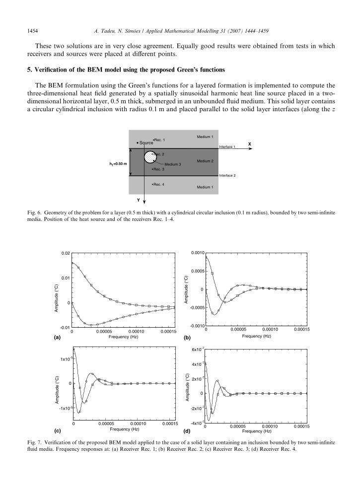
The BEM formulation using the Green’s functions for a layered formation is implemented to compute thethree-dimensional heat field generated by a spatially sinusoidal harmonic heat line source placed in a two-dimensional horizontal layer, 0.5 m thick, submerged in an unbounded fluid medium. This solid layer containsa circular cylindrical inclusion with radius 0.1 m and placed parallel to the solid layer interfaces (along the z

X

Medium 1

Medium 1

h1=0.50 m

Y

Interface 1

Interface 2

Rec. 3

Rec. 4

Medium 3Medium 2

Rec. 2

• SourceRec. 1

Fig. 6. Geometry of the problem for a layer (0.5 m thick) with a cylindrical circular inclusion (0.1 m radius), bounded by two semi-infinitemedia. Position of the heat source and of the receivers Rec. 1–4.

-0.01

0

0.01

0.02

0 0.00005 0.00010 0.00015Frequency (Hz)

Am

plitu

de (

°C)

Am

plitu

de (

°C)

Am

plitu

de (

°C)

-0.0010

-0.0005

0

0.0005

0.0010

0 0.00005 0.00010 0.00015

Frequency (Hz)

-1x10-5

0

1x10-5

0 0.00005 0.00010 0.00015Frequency (Hz)

Am

plitu

de (

°C)

-4x10-7

-2x10-7

0

2x10-7

4x10-7

6x10-7

0 0.00005 0.00010 0.00015Frequency (Hz)

(a) (b)

(c) (d)

Fig. 7. Verification of the proposed BEM model applied to the case of a solid layer containing an inclusion bounded by two semi-infinitefluid media. Frequency responses at: (a) Receiver Rec. 1; (b) Receiver Rec. 2; (c) Receiver Rec. 3; (d) Receiver Rec. 4.


direction) (see Fig. 6). Incorporating the Green’s functions, derived above, into the BEM formulation, the dis-cretization is limited to the inclusion surface. The solutions obtained are compared with those given by theBEM formulation which uses the Green’s functions only for the unbounded media and requires the additionaldiscretization of the flat interfaces.

The properties and the assumed convection velocities of media 1 and 2 are the same as those used in ver-ification section above, while the thermal properties and the convection velocity in the inclusion are assumedto be k3 = 0.12 W m�1 �C�1, c3 = 1380.0 J kg�1 �C�1 and q3 = 510 kg m�3 and �2 · 10�7 m/s, respectively.This system is heated by a harmonic line source located at (x = �0.1 m, y = �0.1 m). All the calculationsare also performed in the frequency range [0, 32 · 0.5 · 10�5 Hz] with a frequency increment of Dx = 10�5 Hzincluding a complex component given by g (g = 0.7Dx). Fig. 7 displays the real and imaginary parts of theresponses at receivers 1–4 when kz = 0.4 rad/m. The receivers Rec. 1–4 are placed at (x = 0.1 m,y = �0.15 m), (x = 0.1 m, y = 0.1 m), (x = 0.1 m, y = 0.35 m) and (x = 0.1 m, y = 0.6 m), respectively.

The solid lines represent responses of the proposed formulation, while the marks correspond to the BEMsolutions using the full boundary discretization. The square and round marks indicate the real and imaginaryparts of the BEM responses, respectively. The standard BEM uses 250 constant boundary elements to modelthe layer interfaces and the inclusion boundary, while the proposed model uses only 50 constant boundaryelements to discretize the inclusion. All the plots reveal an excellent agreement between the two solutionspresented.

6. Applications

In order to illustrate the applicability of the formulation presented above, several simulations have beenperformed. They use a layered system built with a solid concrete layer (medium 2) containing three inclusions(medium 3), and buried in two semi-infinite water media (medium 1). Inside the solid layer, 0.3 m thick, threecylindrical circular inclusions with 0.055 m of radius are modelled, as shown in Fig. 8a. The semi-infinite watermedia were assumed to allow both conduction and convection phenomena, while only the conduction phe-nomenon exists in the solid layer. This process assumes that there is an inflowing mass along the top of theupper and the bottom of the lower boundaries that verifies the mass conservation.

Two different systems are modelled: in the first (Case 1) the inclusions are made of polystyrene (with ther-mal properties k = 0.027 W m�1 �C�1, c = 1210 J kg�1 �C�1 and q = 55 kg m�3); in the second (Case 2) steelproperties (with thermal properties k = 63.9 W m�1 �C�1, c = 434.0 J kg�1 �C�1 and q = 7832.0 kg m�3) wereprescribed for the inclusions. The vertical convection velocities allowed at the top and bottom water mediumwere 2 · 10�6 m/s and 1 · 10�6 m/s, respectively.

The thermal conductivity, specific heat and density of the concrete layer are k = 1.4 W m�1 �C�1,c = 880 J kg�1 �C�1 and q = 2300 kg m�3, respectively. The thermal properties of the top and bottom

X

Medium 1

Medium 1

h1=0.30 m

Interface 1

Interface 2

Medium 2

0.1 m

Y

Rec. 1

Rec. 2

Rec. 3Medium 3

Heat plane source

2 10 mytV −6

−6

= ×

1 10 m/sybV = ×

0 5 10 15 20 250

200

400

600

800

1000

1200

Time (h)

Sou

rce

pow

er (

W)

/s

(a) (b)

Fig. 8. Geometry and source power information of the problem: (a) Solid layer with three circular cylindrical inclusions, bounded by twounbounded fluid media; (b) Heating curve of the source.

Case 1 Case 2

-0.5 0 0.5-0.1

0

0.1

0.2

0.3

0.4

20

3

0.5

1510

0.1

1.5

5

0.25

124

7.5

y(m

)

-0.5 0 0.5-0.1

0

0.1

0.2

0.3

0.4

20

3

0.5

1510

7.5

0.1

1.5

5

0.25

1

2

4y(m

)-0.5 0 0.5

-0.1

0

0.1

0.2

0.3

0.4

10

1.5

3

7.5

5

2

4

y(m

)

-0.5 0 0.5-0.1

0

0.1

0.2

0.3

0.4

10

3

7.5

1.5

54

2

x(m)x(m)

x(m)x(m)

y(m

)

(a)

(b)

Fig. 9. Distribution of temperature registered at a grid of receivers for a homogeneous concrete layer with circular inclusions ofpolystyrene (Case1) and steel (Case2), when convection velocity is ascribed to the top and bottom media: (a) t = 10 h; (b) t = 20 h.


unbounded media were kept constant and similar to those of the water: k = 0.606 W m�1 �C�1,c = 4181 J kg�1 �C�1 and q = 998.0 kg m�3.

The calculations are first performed in the frequency domain [0, 128 · 0.5 · 10�5 Hz], with a frequencyincrement of 0.5 · 10�5 Hz. This defines a time window with a total duration of 55.56 h. Null initial temper-atures and heat fluxes are prescribed along the full domain.

These systems were subjected to a plane heat source placed in the lower medium (y0 = �0.1 m). The energyemitted by the plane heat source was assumed to have a trapezoidal evolution, as shown in Fig. 8b. The heatsource starts emitting energy at t � 0.76 h and its power is increased linearly from 0.0 W to 1000.0 W, reachingmaximum power at t � 3.46 h; the source keeps introducing heat into the system, continuously, for a period oft � 2.72 h; the power then falls linearly; it reaches 0.0 W at t � 8.89 h. Note that different temporal powersource evolutions could be easily implemented.

Fig. 9 presents contour plots obtained at t = 10 h and t = 20 h, using the temperature amplitudes obtainedover a fine grid of receivers. The convection phenomenon is modelled assuming that its origin coincides withthe position of the heat source. The marked differences observed between the computations performed forCase 1 and Case 2 scenarios are attributed to the different thermal properties of the inclusions, since the restof system remains the same. The temperature curves in the presence of the polystyrene inclusions (Case 1)reveal higher temperatures at the bottom of the inclusions and lower temperatures behind the inclusion whencompared with the Case 2 (steel inclusions). The energy being accumulated at the source side of the inclusions,observed in the Case 1, is due to the low thermal diffusivity coefficient of the polystyrene.

For comparison, Fig. 10 displays similar results computed when no convection is allowed in the fluid media.Comparing the two cases in Figs. 9 and 10 at t = 10 h, it is interesting to note that the heat spreads faster whenpositive vertical convection velocities are ascribed to the top and bottom media. Higher temperatures aretherefore registered along the solid media. At t = 20 h, the heating sources are already switched off. However,as can be seen for both cases analysed, the energy is still propagating across the domain, since the heat equi-librium is not completed.

To better illustrate the time evolution of the heat diffusion, the results computed at three receivers areshown in Fig. 11. The receivers Rec. 1, Rec. 2 and Rec. 3 are placed at (x = 0.0 m, y = 0.073 m),(x = 0.0 m, y = 0.145 m) and (x = 0.0 m, y = 0.216 m), respectively, as displayed in Fig. 8a.

Case 1 Case 2

-0.5 0 0.5-0.1

0

0.1

0.2

0.3

0.4

20

4

1

0.05

1510

0.25

2

7.5

0.1

0.5

1.5

35

y(m

)

-0.5 0 0.5-0.1

0

0.1

0.2

0.3

0.4

20

4

1

0.05

15 10

0.25

2

7.5

0.1

0.5

1.535

y(m

)-0.5 0 0.5

-0.1

0

0.1

0.2

0.3

0.4

10

21

7.5

45

1.53

x(m) x(m)

x(m)x(m)

y(m

)

-0.5 0 0.5-0.1

0

0.1

0.2

0.3

0.4

15

1.5

5

10

0.5

7.5

3

12

4

y(m

)

(a)

(b)

Fig. 10. Distribution of temperature registered at a grid of receivers for a homogeneous concrete layer with circular inclusions ofpolystyrene (Case1) and steel (Case2), considering only the conduction phenomenon: (a) t = 10 h; (b) t = 20 h.

Conduction phenomenon Conduction and convection phenomena

0 5 10 15 20 250

5

10

15

Time (h)

Tem

pera

ture

(°c

)

Rec. 1Rec. 2Rec. 3

0 5 10 15 20 250

5

10

15

Time (h)

Tem

pera

ture

(°c

)

Rec. 1Rec. 2Rec. 3

0 5 10 15 20 250

5

10

15

Time (h)

Tem

pera

ture

(°c

)

Rec. 1Rec. 2Rec. 3

0 5 10 15 20 250

5

10

15

Time (h)

Tem

pera

ture

(°c

)

Rec. 1Rec. 2Rec. 3

(a)

(b)

Fig. 11. Temperature evolution at the receivers Rec. 1, 2 and 3: (a) Case 1 (polystyrene inclusions); (b) Case 2 (steel inclusions).



The receiver Rec.1, which is closer to the position of the heat plane source, is the first to record a progres-sive change of temperature. The higher temperatures registered at the Rec. 1 when the inclusion is made ofpolystyrene (Case 1) confirm its insulating properties. The receiver placed inside the polystyrene inclusion alsorecords higher temperatures than those registered in the steel inclusion, because the energy does not propagateeasily through this material. Notice also that, the receiver located immediately behind the inclusion (receiver 3)registers lower temperatures when the inclusion is made of polystyrene (Case 1).

The results illustrated in Fig. 11 show that, in the time window being studied, only the receiver nearest theheat source records a fall in temperature after the source power has dropped to 0 W. In fact, the temperature isstill increasing at the receivers placed further away from the heat source. The energy equilibrium along thedomain takes a long time to be established, as can be predicted from the results obtained for a time windowof 25.55 h.

The modelling of the positive convection velocity along the y direction introduces marked differences in thethermal response along the domain. For example the receiver Rec. 1 registers a maximum temperature of11.4 �C when both conduction and convection phenomena are modelled, while the same receiver in the pres-ence of the conduction alone records a temperature of 9.75 �C. The presence of the convection enables the heatto flow faster, and so the temperature falls sooner.

Once the source has reached the maximum power, the differences between the temperatures registered at thereceivers is seen to be higher in the presence of the extruded polystyrene inclusions (Case 1). The oppositebehaviour (small thermal gradient) is found in Case 2 because the steel allows higher thermal diffusivity.The temperature variation inside the steel inclusion is very small; as a consequence, the temperature curvefor Rec. 2 and 3 are very close and similar (see Fig. 11b).

Finally, it is important to remember that the heat transfer across a layer formation can be affected to a con-siderable extent by the presence of thermal heterogeneities and the convection phenomenon. The proposedformulation can help to model this kind of problem with greater efficiency.

7. Conclusions

The transient heat transfer by conduction and convection across a solid layer with heterogeneities, boundedby two semi-infinite media has been described.

This paper has illustrated how heat diffusion can be determined in the frequency domain, reformulating themathematical and numerical formulations found in other fields such as wave problems. The BEM techniqueproposed can handle any type of heat source and allows the modelling of layered media without having todiscretize the solid interfaces. A series of verifications were performed to assure the formulation’s accuracy:the verification of the frequency domain approach using the Green’s functions for the unbounded medium;the verification of the Green’s functions for a layered formation; and the verification of the formulation basedon a BEM model that includes the Green’s functions for the layered formation.

The proposed formulation was used to compute the temperature distribution evolution for a solid layercontaining several thermal heterogeneities. Different thermal properties were prescribed for the inclusionsand both the conduction and convection phenomena were modelled. The results obtained demonstrate theparticular importance of the convection phenomenon, and the marked influence of the thermal heterogeneitieson the heat transfer across a layered formation.

References

[1] C.A. Brebbia, J.C.F. Telles, L.C. Wrobel, Boundary Element Techniques: Theory and Applications in Engineering, Springer, Berlin,1984.

[2] M.L.G. Pina, J.L.M. Fernandez, Applications in heat conduction by BEM, in: C.A. Brebbia (Ed.), Topics in Boundary ElementResearch, Springer, Berlin, 1984.

[3] Y.P. Chang, C.S. Kang, D.J. Chen, The use of fundamental Green’s functions for solution of problems of heat conduction inanisotropic media, Int. J. Heat Mass Transfer 16 (1973) 1905–1918.

[4] R.P. Shaw, An integral equation approach to diffusion, Int. J. Heat Mass Transfer 17 (1974) 693–699.[5] L.C. Wrobel, C.A. Brebbia, A formulation of the boundary element method for axisymmetric transient heat conduction, Int. J. Heat

Mass Transfer 24 (1981) 843–850.


[6] A. Carini, M. Diligenti, A. Salvadori, Implementation of a symmetric boundary element method in transient heat conduction withsemi-analytical integrations, Int. J. Numer. Methods Eng. 46 (1999) 1819–1843.

[7] D. Lesnic, L. Elliot, D.B. Ingham, Treatment of singularities in time-dependent problems using the boundary element method, Eng.Anal. Bound. Elem. EABE 16 (1995) 65–70.

[8] A. Sutradhar, G.H. Paulino, L.J. Gray, Transient heat conduction in homogeneous and non-homogeneous materials by the Laplacetransform Galerkin boundary element method, Eng. Anal. Bound. Elem. EABE 26 (2) (2002) 119–132.

[9] A. Sutradhar, G.H. Paulino, The simple boundary element method for transient heat conduction in functionally graded materials,Comput. Methods Appl. Mech. Eng. 193 (2004) 4511–4539.

[10] D. Nardini, C.A. Brebbia, A new approach to free vibration analysis using boundary elements, Boundary Element Methods inEngineering, Computational Mechanics Publications/Springer-Verlag, Southampton/Berlin, 1982.

[11] S.P. Zhu, P. Satravaha, An efficient computational method for nonlinear transient heat conduction problems, Appl. Math. Model. 20(1996) 513–522.

[12] P. Satravaha, S. Zhu, An application of the LTDRM to transient diffusion problems with nonlinear material properties and nonlinearboundary conditions, Appl. Math. Comput. 87 (1997) 127–160.

[13] I. Guven, E. Madenci, Transient heat conduction analysis in a piecewise homogeneous domain by a coupled boundary and finiteelement method, Int. J. Numer. Methods. Eng. 56 (2003) 351–380.

[14] M. Tanaka, K. Tanaka, Transient heat conduction problems in inhomogeneous media discretized by means of boundary volumeelement, Nucl. Eng. Des. 60 (1980) 381–387.

[15] R. Butterfield, An application of the boundary element method to potential flow problems in generally inhomogeneous bodies, in:C.A. Brebbia (Ed.), Recent Advances in Boundary Element Method, Pentech Press, London, 1978.

[16] J. Sladek, V. Sladek, Ch. Zhang, A local BIEM for analysis of transient heat conduction with nonlinear source terms in FGMs, Eng.Anal. Bound. Elem. EABE 28 (2004) 1–11.

[17] A. Tadeu, J. Antonio, L. Godinho, N. Simoes, Boundary element method analyses of transient heat conduction in an unboundedsolid layer containing inclusions, Comput. Mech. 34 (2004) 99–110.

[18] H. Lamb, On the propagation of tremors at the surface of an elastic solid, Philos. Trans. Roy. Soc. London A203 (1904) 1–42.[19] M. Bouchon, Discrete wave number representation of elastic wave fields in three-space dimensions, J. Geophys. Res. 84 (1979) 3609–

3614.[20] A. Tadeu, J. Antonio, 2.5D Green’s functions for elastodynamic problems in layered acoustic and elastic formations, J. Comput.

Model. Eng. Sci. CMES 2 (4) (2001) 477–495.[21] P.K. Banerjee, The Boundary Element Methods in Engineering, McGraw-Hill, England, 1981.[22] H.S. Carslaw, J.C. Jaeger, Conduction of Heat in Solids, second ed., Oxford University Press, 1959.[23] Gradshteyn, Ryzhik, Tables of integrals, series, and products, 1980.[24] L. Schwartz, Theorie des distributions, Hermann, Paris, 1966.[25] M. Bouchon, K. Aki, Time-domain transient elastodynamic analysis of 3D solids by BEM, Int. J. Numer. Methods Eng. 26 (1977)

1709–1728.[26] A. Tadeu, L. Godinho, P. Santos, Wave motion between two fluid filled boreholes in an elastic medium, Eng. Anal. Bound. Elem.

EABE 26 (2) (2002) 101–117.[27] L. Godinho, J. Antonio, A. Tadeu, 3D sound scattering by rigid barriers in the vicinity of tall buildings, J. Appl. Acoust. 62 (11)

(2001) 1229–1248.[28] W. Garvin, Exact transient solution of the buried line source problem, Proc. Roy. Soc. London, Ser. A – Math. Phys. Sci. 234 (1199)

(1955) 528–541.[29] P.M. Morse, Feshbach Methods of Theoretical Physics, McGraw-Hill, New York, 1953, p. 823.[30] E. Kausel, J.M. Roesset, Frequency domain analysis of undamped systems, J. Eng. Mech. ASCE 118 (4) (1992) 721–734.[31] A. Tadeu, P. Santos, E. Kausel, Closed-form integration of singular terms for constant, linear and quadratic boundary elements –

Part I: SH wave propagation, Eng. Anal. Bound. Elem. EABE 23 (8) (1999) 671–681.[32] A. Tadeu, P. Santos, E. Kausel, Closed-form integration of singular terms for constant, linear and quadratic boundary elements –

Part II: SV-P wave propagation, Eng. Anal. Bound. Elem. EABE 23 (9) (1999) 757–768.[33] R.A. Phinney, Theoretical calculation of the spectrum of first arrivals in the layered elastic medium, J. Geophys. Res. 70 (1965) 5107–

5123.

conduction and convection phenomena through a … · conduction and convection phenomena through a...

Documents