Conditional Random Fields as Recurrent Neural Networks

Shuai Zheng1* Sadeep Jayasumana1∗ Bernardino Romera-Paredes1 Vibhav Vineet1,2†

Zhizhong Su3 Dalong Du3 Chang Huang3 Philip H. S. Torr1

1Torr-Vision Group, University of Oxford 2Stanford University 3Baidu Research

Abstract

Pixel-level labelling tasks, such as semantic segmenta-

tion, play a central role in image understanding. Recent ap-

proaches have attempted to harness the capabilities of deep

learning techniques for image recognition to tackle pixel-

level labelling tasks. One central issue in this methodology

is the limited capacity of deep learning techniques to de-

lineate visual objects. To solve this problem, we introduce

a new form of convolutional neural network that combines

the strengths of Convolutional Neural Networks (CNNs)

and Conditional Random Fields (CRFs)-based probabilis-

tic graphical modelling. To this end, we formulate Con-

ditional Random Fields with Gaussian pairwise potentials

and mean-field approximate inference as Recurrent Neural

Networks. This network, called CRF-RNN, is then plugged

in as a part of a CNN to obtain a deep network that has

desirable properties of both CNNs and CRFs. Importantly,

our system fully integrates CRF modelling with CNNs, mak-

ing it possible to train the whole deep network end-to-end

with the usual back-propagation algorithm, avoiding offline

post-processing methods for object delineation.

We apply the proposed method to the problem of seman-

tic image segmentation, obtaining top results on the chal-

lenging Pascal VOC 2012 segmentation benchmark.

1. Introduction

Low-level computer vision problems such as semantic

image segmentation or depth estimation often involve as-

signing a label to each pixel in an image. While the feature

representation used to classify individual pixels plays an im-

portant role in this task, it is similarly important to consider

factors such as image edges, appearance consistency and

spatial consistency while assigning labels in order to obtain

accurate and precise results.

Designing a strong feature representation is a key chal-

lenge in pixel-level labelling problems. Work on this topic

∗Authors contributed equally.†Work conducted while author at the University of Oxford.

includes: TextonBoost [50], TextonForest [49], and Ran-

dom Forest-based classifiers [48]. Recently, supervised

deep learning approaches such as large-scale deep Convolu-

tional Neural Networks (CNNs) have been immensely suc-

cessful in many high-level computer vision tasks such as

image recognition [29] and object detection [19]. This mo-

tivates exploring the use of CNNs for pixel-level labelling

problems. The key insight is to learn a strong feature rep-

resentation end-to-end for the pixel-level labelling task in-

stead of hand-crafting features with heuristic parameter tun-

ing. In fact, a number of recent approaches including the

particularly interesting works FCN [35] and DeepLab [9]

have shown a significant accuracy boost by adapting state-

of-the-art CNN based image classifiers to the semantic seg-

mentation problem.

However, there are significant challenges in adapting

CNNs designed for high level computer vision tasks such as

object recognition to pixel-level labelling tasks. Firstly, tra-

ditional CNNs have convolutional filters with large recep-

tive fields and hence produce coarse outputs when restruc-

tured to produce pixel-level labels [35]. Presence of max-

pooling layers in CNNs further reduces the chance of get-

ting a fine segmentation output [9]. This, for instance, can

result in non-sharp boundaries and blob-like shapes in se-

mantic segmentation tasks. Secondly, CNNs lack smooth-

ness constraints that encourage label agreement between

similar pixels, and spatial and appearance consistency of the

labelling output. Lack of such smoothness constraints can

result in poor object delineation and small spurious regions

in the segmentation output [57, 56, 30, 37].

On a separate track to the progress of deep learning

techniques, probabilistic graphical models have been devel-

oped as effective methods to enhance the accuracy of pixel-

level labelling tasks. In particular, Markov Random Fields

(MRFs) and its variant Conditional Random Fields (CRFs)

have observed widespread success in this area [30, 27] and

have become one of the most successful graphical models

used in computer vision. The key idea of CRF inference

for semantic labelling is to formulate the label assignment

problem as a probabilistic inference problem that incor-

porates assumptions such as the label agreement between

43211529

similar pixels. CRF inference is able to refine weak and

coarse pixel-level label predictions to produce sharp bound-

aries and fine-grained segmentations. Therefore, intuitively,

CRFs can be used to overcome the drawbacks in utilizing

CNNs for pixel-level labelling tasks.

One way to utilize CRFs to improve the semantic la-

belling results produced by a CNN is to apply CRF infer-

ence as a post-processing step disconnected from the train-

ing of the CNN [9]. Arguably, this does not fully harness

the strength of CRFs since it is not integrated with the deep

network – the deep network cannot adapt its weights to the

CRF behaviour during the training phase.

In this paper, we propose an end-to-end deep learn-

ing solution for the pixel-level semantic image segmenta-

tion problem. Our formulation combines the strengths of

both CNNs and CRF based graphical models in one unified

framework. More specifically, we formulate mean-field in-

ference of dense CRF with Gaussian pairwise potentials as

a Recurrent Neural Network (RNN) which can refine coarse

outputs from a traditional CNN in the forward pass, while

passing error differentials back to the CNN during train-

ing. Importantly, with our formulation, the whole deep net-

work, which comprises a traditional CNN and an RNN for

CRF inference, can be trained end-to-end utilizing the usual

back-propagation algorithm.

Arguably, when properly trained, the proposed network

should outperform a system where CRF inference is applied

as a post-processing method on independent pixel-level pre-

dictions produced by a pre-trained CNN. Our experimental

evaluation confirms that this indeed is the case.

2. Related Work

In this section we review approaches that make use of

deep learning and CNNs for low-level computer vision

tasks, with a focus on semantic image segmentation. A wide

variety of approaches have been proposed to tackle the se-

mantic image segmentation task using deep learning. These

approaches can be categorized into two main strategies.

The first strategy is based on utilizing separate mecha-

nisms for feature extraction, and image segmentation ex-

ploiting the edges of the image [2, 36]. One representative

instance of this scheme is the application of a CNN for the

extraction of meaningful features, and using superpixels to

account for the structural pattern of the image. Two repre-

sentative examples are [18, 36], where the authors first ob-

tained superpixels from the image and then used a feature

extraction process on each of them. The main disadvantage

of this strategy is that errors in the initial proposals (e.g:

super-pixels) may lead to poor predictions, no matter how

good the feature extraction process is. Pinheiro and Col-

lobert [44] employed an RNN to model the spatial depen-

dencies during scene parsing. In contrast to their approach,

we show that a typical graphical model such as a CRF can

be formulated as an RNN to form a part of a deep network,

to perform end-to-end training combined with a CNN.

The second strategy is to directly learn a nonlinear model

from the images to the label map. This, for example, was

shown in [16], where the authors replaced the last fully con-

nected layers of a CNN by convolutional layers to keep spa-

tial information. An important contribution in this direction

is [35], where Long et al. used the concept of fully con-

volutional networks, and the notion that top layers obtain

meaningful features for object recognition whereas low lay-

ers keep information about the structure of the image, such

as edges. In their work, connections from early layers to

later layers were used to combine these cues. Bell et al. [5]

and Chen et al. [9, 39] used a CRF to refine segmentation

results obtained from a CNN. Bell et al. focused on material

recognition and segmentation, whereas Chen et al. reported

very significant improvements on semantic image segmen-

tation. In contrast to these works, which employed CRF

inference as a standalone post-processing step disconnected

from the CNN training, our approach is an end-to-end train-

able network that jointly learns the parameters of the CNN

and the CRF in one unified deep network.

Works that use neural networks to predict structured out-

put are found in different domains. For example, Do et

al. [13] proposed an approach to combine deep neural net-

works and Markov networks for sequence labeling tasks.

Another domain which benefits from the combination of

CNNs and structured loss is handwriting recognition. In [6],

the authors combined a CNN with Hidden Markov Models

for that purpose, whereas more recently, Peng et al. [43]

used a modified version of CRFs. Related to this line of

works, in [24] a joint CNN and CRF model was used for

text recognition on natural images. Tompson et al. [55]

showed the use of joint training of a CNN and an MRF for

human pose estimation, while Chen et al. [10] focused on

the image classification problem with a similar approach.

Another prominent work is [20], in which the authors ex-

press Deformable Part Models, a kind of MRF, as a layer

in a neural network. In our approach we cast a different

graphical model as a neural network layer.

A number of approaches have been proposed for au-

tomatic learning of graphical model parameters and joint

training of classifiers and graphical models. Barbu et al. [4]

proposed a joint training of a MRF/CRF model together

with an inference algorithm in their Active Random Field

approach. Domke [14] advocated back-propagation based

parameter optimization in graphical models when approxi-

mate inference methods such as mean-field and belief prop-

agation are used. This idea was utilized in [26], where a bi-

nary dense CRF was used for human pose estimation. Sim-

ilarly, Ross et al. [45] and Stoyanov et al. [52] showed how

back-propagation through belief propagation can be used to

optimize model parameters. Ross et al. [45], in particular,

1530

proposed an approach based on learning messages. Many

of these ideas can be traced back to [53], which proposed

unrolling message passing algorithms as simpler operations

that could be performed within a CNN. In a different setup,

Krahenbuhl and Koltun [28] demonstrated automatic pa-

rameter tuning of dense CRF when a modified mean-field

algorithm is used for inference. An alternative inference ap-

proach for dense CRF, not based on mean-field, is proposed

in [58].

In contrast to the works described above, our approach

shows that it is possible to formulate dense CRF as an RNN

so that one can form an end-to-end trainable system for se-

mantic image segmentation which combines the strengths

of deep learning and graphical modelling. The concurrent

and independent work [47] explores a similar joint training

approach for semantic segmentation.

3. Conditional Random Fields

In this section we provide a brief overview of CRF for

pixel-wise labelling and introduce the notation used in the

paper. A CRF, used in the context of pixel-wise label pre-

diction, models pixel labels as random variables that form

a MRF when conditioned upon a global observation. The

global observation is usually taken to be the image.

Let Xi be the random variable associated to pixel i,

which represents the label assigned to the pixel i and

can take any value from a pre-defined set of labels L ={l1, l2, . . . , lL}. Let X be the vector formed by the ran-

dom variables X1, X2, . . . , XN , where N is the number of

pixels in the image. Given a graph G = (V,E), where

V = {X1, X2, . . . , XN}, and a global observation (im-

age) I, the pair (I,X) can be modelled as a CRF charac-

terized by a Gibbs distribution of the form P (X = x|I) =1

Z(I) exp(−E(x|I)). Here E(x) is called the energy of

the configuration x ∈ LN and Z(I) is the partition func-

tion [31]. From now on, we drop the conditioning on I in

the notation for convenience.

In the fully connected pairwise CRF model of [27], the

energy of a label assignment x is given by:

E(x) =∑

i

ψu(xi) +∑

i<j

ψp(xi, xj), (1)

where the unary energy components ψu(xi) measure the

inverse likelihood (and therefore, the cost) of the pixel

i taking the label xi, and pairwise energy components

ψp(xi, xj) measure the cost of assigning labels xi, xj to

pixels i, j simultaneously. In our model, unary energies are

obtained from a CNN, which, roughly speaking, predicts la-

bels for pixels without considering the smoothness and the

consistency of the label assignments. The pairwise ener-

gies provide an image data-dependent smoothing term that

encourages assigning similar labels to pixels with similar

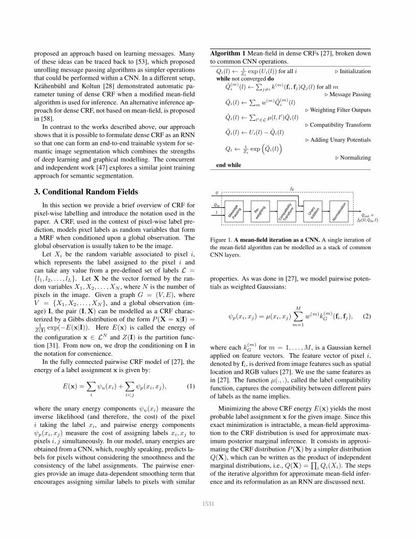
Algorithm 1 Mean-field in dense CRFs [27], broken down

to common CNN operations.

Qi(l)←1Zi

exp (Ui(l)) for all i ⊲ Initialization

while not converged do

Q(m)i (l)←

∑

j 6=ik(m)(fi, fj)Qj(l) for all m

⊲ Message Passing

Qi(l)←∑

mw(m)Q

(m)i (l)

⊲ Weighting Filter Outputs

Qi(l)←∑

l′∈L µ(l, l′)Qi(l)⊲ Compatibility Transform

Qi(l)← Ui(l)− Qi(l)⊲ Adding Unary Potentials

Qi ←1Zi

exp(

Qi(l))

⊲ Normalizing

end while

Figure 1. A mean-field iteration as a CNN. A single iteration of

the mean-field algorithm can be modelled as a stack of common

CNN layers.

properties. As was done in [27], we model pairwise poten-

tials as weighted Gaussians:

ψp(xi, xj) = µ(xi, xj)M∑

m=1

w(m)k(m)G (fi, fj), (2)

where each k(m)G for m = 1, . . . ,M , is a Gaussian kernel

applied on feature vectors. The feature vector of pixel i,

denoted by fi, is derived from image features such as spatial

location and RGB values [27]. We use the same features as

in [27]. The function µ(., .), called the label compatibility

function, captures the compatibility between different pairs

of labels as the name implies.

Minimizing the above CRF energy E(x) yields the most

probable label assignment x for the given image. Since this

exact minimization is intractable, a mean-field approxima-

tion to the CRF distribution is used for approximate max-

imum posterior marginal inference. It consists in approxi-

mating the CRF distribution P (X) by a simpler distribution

Q(X), which can be written as the product of independent

marginal distributions, i.e., Q(X) =∏

iQi(Xi). The steps

of the iterative algorithm for approximate mean-field infer-

ence and its reformulation as an RNN are discussed next.

1531

4. A Mean-field Iteration as a Stack of CNN

Layers

A key contribution of this paper is to show that the mean-

field CRF inference can be reformulated as a Recurrent

Neural Network (RNN). To this end, we first consider in-

dividual steps of the mean-field algorithm summarized in

Algorithm 1 [27], and describe them as CNN layers. Our

contribution is based on the observation that filter-based ap-

proximate mean-field inference approach for dense CRFs

relies on applying Gaussian spatial and bilateral filters on

the mean-field approximates in each iteration. Unlike the

standard convolutional layer in a CNN, in which filters are

fixed after the training stage, we use edge-preserving Gaus-

sian filters [54, 40], coefficients of which depend on the

original spatial and appearance information of the image.

These filters have the additional advantages of requiring a

smaller set of parameters, despite the filter size being po-

tentially as big as the image.

While reformulating the steps of the inference algorithm

as CNN layers, it is essential to be able to calculate er-

ror differentials in each layer w.r.t. its inputs in order to

be able to back-propagate the error differentials to previous

layers during training. We also discuss how to calculate er-

ror differentials w.r.t. the parameters in each layer, enabling

their optimization through the back-propagation algorithm.

Therefore, in our formulation, CRF parameters such as the

weights of the Gaussian kernels and the label compatibil-

ity function can also be optimized automatically during the

training of the full network.

Once the individual steps of the algorithm are broken

down as CNN layers, the full algorithm can then be for-

mulated as an RNN. We explain this in Section 5 after dis-

cussing the steps of Algorithm 1 in detail below. In Algo-

rithm 1 and the remainder of this paper, we use Ui(l) to

denote the negative of the unary energy introduced in the

previous section, i.e., Ui(l) = −ψu(Xi = l). In the con-

ventional CRF setting, this input Ui(l) to the mean-field al-

gorithm is obtained from an independent classifier.

4.1. Initialization

In the initialization step of the algorithm, the operation

Qi(l) ←1Zi

exp (Ui(l)), where Zi =∑

l exp(Ui(l)), is

performed. Note that this is equivalent to applying a soft-

max function over the unary potentials U across all the la-

bels at each pixel. The softmax function has been exten-

sively used in CNN architectures before and is therefore

well known in the deep learning community. This operation

does not include any parameters and the error differentials

received at the output of the step during back-propagation

could be passed down to the unary potential inputs after per-

forming usual backward pass calculations of the softmax

transformation.

4.2. Message Passing

In the dense CRF formulation of [27], message passing

is implemented by applying M Gaussian filters on Q val-

ues. Gaussian filter coefficients are derived based on image

features such as the pixel locations and RGB values, which

reflect how strongly a pixel is related to other pixels. Since

the CRF is potentially fully connected, each filter’s recep-

tive field spans the whole image, making it infeasible to use

a brute-force implementation of the filters. Fortunately, sev-

eral approximation techniques exist to make computation

of high dimensional Gaussian filtering significantly faster.

Following [27], we use the permutohedral lattice implemen-

tation [1], which can compute the filter response in O(N)time, where N is the number of pixels of the image [1].

During back-propagation, error derivatives w.r.t. the fil-

ter inputs are calculated by sending the error derivatives

w.r.t. the filter outputs through the same M Gaussian fil-

ters in reverse direction. In terms of permutohedral lattice

operations, this can be accomplished by only reversing the

order of the separable filters in the blur stage, while building

the permutohedral lattice, splatting, and slicing in the same

way as in the forward pass. Therefore, back-propagation

through this filtering stage can also be performed in O(N)time. Following [27], we use two Gaussian kernels, a spa-

tial kernel and a bilateral kernel. In this work, for simplicity,

we keep the bandwidth values of the filters fixed.

4.3. Weighting Filter Outputs

The next step of the mean-field iteration is taking a

weighted sum of theM filter outputs from the previous step,

for each class label l. When each class label is considered

individually, this can be viewed as usual convolution with

a 1 × 1 filter with M input channels, and one output chan-

nel. Since both inputs and the outputs to this step are known

during back-propagation, the error derivative w.r.t. the filter

weights can be computed, making it possible to automat-

ically learn the filter weights (relative contributions from

each Gaussian filter output from the previous stage). Er-

ror derivative w.r.t. the inputs can also be computed in the

usual manner to pass the error derivatives down to the previ-

ous stage. To obtain a higher number of tunable parameters,

in contrast to [27], we use independent kernel weights for

each class label. The intuition is that the relative importance

of the spatial kernel vs the bilateral kernel depends on the

visual class. For example, bilateral kernels may have on the

one hand a high importance in bicycle detection, because

similarity of colours is determinant; on the other hand they

may have low importance for TV detection, given that what-

ever is inside the TV screen may have different colours.

4.4. Compatibility Transform

In the compatibility transform step, outputs from the pre-

vious step (denoted by Q in Algorithm 1) are shared be-

1532

tween the labels to a varied extent, depending on the com-

patibility between these labels. Compatibility between the

two labels l and l′ is parameterized by the label compatibil-

ity function µ(l, l′). The Potts model, given by µ(l, l′) =[l 6= l′], where [.] is the Iverson bracket, assigns a fixed

penalty if different labels are assigned to pixels with simi-

lar properties. A limitation of this model is that it assigns

the same penalty for all different pairs of labels. Intuitively,

better results can be obtained by taking the compatibility

between different label pairs into account and penalizing

the assignments accordingly. For example, assigning la-

bels “person” and “bicycle” to nearby pixels should have

a lesser penalty than assigning “sky” and “bicycle”. There-

fore, learning the function µ from data is preferred to fixing

it in advance with Potts model. We also relax our compat-

ibility transform model by assuming µ(l, l′) 6= µ(l′, l) in

general.

Compatibility transform step can be viewed as another

convolution layer where the spatial receptive field of the fil-

ter is 1 × 1, and the number of input and output channels

are both L. Learning the weights of this filter is equivalent

to learning the label compatibility function µ. Transferring

error differentials from the output of this step to the input

can be done since this step is a usual convolution operation.

4.5. Adding Unary Potentials

In this step, the output from the compatibility transform

stage is subtracted element-wise from the unary inputs U .

While no parameters are involved in this step, transferring

error differentials can be done trivially by copying the dif-

ferentials at the output of this step to both inputs with the

appropriate sign.

4.6. Normalization

Finally, the normalization step of the iteration can be

considered as another softmax operation with no parame-

ters. Differentials at the output of this step can be passed on

to the input using the softmax operation’s backward pass.

5. The End-to-end Trainable Network

We now describe our end-to-end deep learning system

for semantic image segmentation. To pave the way for this,

we first explain how repeated mean-field iterations can be

organized as an RNN.

5.1. CRF as RNN

In the previous section, it was shown that one iteration

of the mean-field algorithm can be formulated as a stack of

common CNN layers (see Fig. 1). We use the function fθto denote the transformation done by one mean-field iter-

ation: given an image I , pixel-wise unary potential values

U and an estimation of marginal probabilities Qin from the

FCN CRF-RNN

Figure 2. The End-to-end Trainable Network. Schematic vi-

sualization of our full network which consists of a CNN and the

CNN-CRF network. Best viewed in colour.previous iteration, the next estimation of marginal distribu-

tions after one mean-field iteration is given by fθ(U,Qin, I).The vector θ =

{

w(m), µ(l, l′)}

, m ∈ {1, . . . ,M}, l, l′ ∈{l1, . . . , lL} represents the CRF parameters described in

Section 4.

Multiple mean-field iterations can be implemented by re-

peating the above stack of layers in such a way that each

iteration takesQ value estimates from the previous iteration

and the unary values in their original form. This is equiva-

lent to treating the iterative mean-field inference as a Recur-

rent Neural Network (RNN). The behaviour of the network

is given by the following equations where H1, H2 are hid-

den states, and T is the number of mean-field iterations:

H1(t) =

{

softmax(U), t = 0

H2(t− 1), 0 < t ≤ T,(3)

H2(t) = fθ(U,H1(t), I), 0 ≤ t ≤ T, (4)

Y (t) =

{

0, 0 ≤ t < T

H2(t), t = T.(5)

We name this RNN structure CRF-RNN. Parameters of

the CRF-RNN are same as the mean-field parameters de-

scribed in Section 4 and denoted by θ here. Since the calcu-

lation of error differentials w.r.t. these parameters in a single

iteration was described in Section 4, they can be learnt in the

RNN setting using the standard back-propagation through

time algorithm [46, 38]. It was shown in [27] that the mean-

field iterative algorithm for dense CRF converges in less

than 10 iterations. Furthermore, in practice, after about 5

iterations, increasing the number of iterations usually does

not significantly improve results [27]. Therefore, it does

not suffer from the vanishing and exploding gradient prob-

lem inherent to deep RNNs [7, 41]. This allows us to use a

plain RNN architecture instead of more sophisticated archi-

tectures such as LSTMs in our network.

5.2. Completing the Picture

Our approach comprises a fully convolutional network

stage, which predicts pixel-level labels without consid-

ering structure, followed by a CRF-RNN stage, which

1533

performs CRF-based probabilistic graphical modelling for

structured prediction. The complete system, therefore, uni-

fies strengths of both CNNs and CRFs and is trainable

end-to-end using the back-propagation algorithm [32] and

the Stochastic Gradient Descent (SGD) procedure. During

training, a whole image (or many of them) can be used as

the mini-batch and the error at each pixel output of the net-

work can be computed using an appropriate loss function

such as the softmax loss with respect to the ground truth

segmentation of the image. We used the FCN-8s architec-

ture of [35] as the first part of our network, which provides

unary potentials to the CRF. This network is based on the

VGG-16 network [51] but has been restructured to perform

pixel-wise prediction instead of image classification. The

complete architecture of our network, including the FCN-

8s part can be found in the supplementary material.

In the forward pass through the network, once the com-

putation enters the CRF-RNN after passing through the

CNN stage, it takes T iterations for the data to leave the

loop created by the RNN. Neither the CNN that provides

unary values nor the layers after the CRF-RNN (i.e., the

loss layers) need to perform any computations during this

time since the refinement happens only inside the RNN’s

loop. Once the output Y leaves the loop, next stages of the

deep network after the CRF-RNN can continue the forward

pass. In our setup, a softmax loss layer directly follows the

CRF-RNN and terminates the network.

During the backward pass, once the error differentials

reach the CRF-RNN’s output Y , they similarly spend T it-

erations within the loop before reaching the RNN input U

in order to propagate to the CNN which provides the unary

input. In each iteration inside the loop, error differentials

are computed inside each component of the mean-field it-

eration as described in Section 4. We note that unnecessar-

ily increasing the number of mean-field iterations T could

potentially result in the vanishing and exploding gradient

problems in the CRF-RNN.

6. Implementation Details

In the present section we describe the implementation

details of the proposed network, as well as its training pro-

cess. The high-level architecture of our system, which was

implemented using the popular Caffe [25] deep learning li-

brary, is shown in Fig. 2. Complete architecture of the deep

network can be found in the supplementary material. The

source code and the trained models of our approach will be

made publicly available.

We initialized the first part of the network using the pub-

licly available weights of the FCN-8s network [35]. The

compatibility transform parameters of the CRF-RNN were

initialized using the Potts model, and kernel width and

weight parameters were obtained from a cross-validation

process. We found that such initialization results in faster

convergence of training. During the training phase, param-

eters of the whole network were optimized end-to-end using

the back-propagation algorithm. In particular, we used full

image training described in [35], with learning rate fixed at

10−13 and momentum set to 0.99. These extreme values of

the parameters were used since we employed only one im-

age per batch to avoid reaching memory limits of the GPU.

In all our experiments, during training, we set the num-

ber of mean-field iterations T in the CRF-RNN to 5 to avoid

vanishing/exploding gradient problems and to reduce the

training time. During the test time, iteration count was in-

creased to 10. The effect of this parameter value on the

accuracy is discussed in Section 7.1.

Loss function During the training of the models that

achieved the best results reported in this paper, we used the

standard softmax loss function, that is, the log-likelihood

error function [28]. The standard metric used in the Pascal

VOC challenge is the average intersection over union (IU),

which we also use here to report the results. In our experi-

ments we found that high values of IU on the validation set

were associated to low values of the averaged softmax loss,

to a large extent. We also tried the robust log-likelihood

in [28] as a loss function for training. However, this did not

result in increased accuracy nor faster convergence.

Normalization techniques As described in Section 4,

we use the exponential function followed by pixel-wise nor-

malization across channels in several stages of the CRF-

RNN. Since this operation has a tendency to result in small

gradients with respect to the input when the input value is

large, we conducted several experiments where we replaced

this by a rectified linear unit (ReLU) operation followed by

a normalization across the channels. Our hypothesis was

that this approach may approximate the original operation

adequately while speeding up the training due to improved

gradients. Furthermore, ReLU would induce sparsity on the

probability of labels assigned to pixels, implicitly pruning

low likelihood configurations, which could have a positive

effect. However, this approach did not lead to better results,

obtaining 1% IU lower than that of original setting.

7. Experiments

We present experimental results with the proposed CRF-

RNN framework. We use two datasets: the Pascal VOC

2012 dataset, and the Pascal Context dataset. We use the

Pascal VOC 2012 dataset as it has become the golden stan-

dard to comprehensively evaluate any new semantic seg-

mentation approach. We also use the Pascal Context dataset

to assess how well our approach performs on a dataset with

different characteristics.

Pascal VOC Datasets

In order to evaluate our approach with existing methods un-

der the same circumstances, we conducted two main exper-

1534

Figure 3. Qualitative results on the validation set of Pascal

VOC 2012. FCN [35] is a CNN-based model that does not em-

ploy CRF. Deeplab [9] is a two-stage approach, where the CNN is

trained first, and then CRF is applied on top of the CNN output.

Our approach is an end-to-end trained system that integrates both

CNN and CRF-RNN in one deep network. Best viewed in colour.

iments with the Pascal VOC 2012 dataset, followed by a

qualitative experiment.

In the first experiment, following [35, 36, 39], we used

a training set consisted of VOC 2012 training data (1464

images), and training and validation data of [22], which

amounts to a total of 11,685 images. After removing the

overlapping images between VOC 2012 validation data and

this training dataset, we were left with 346 images from the

original VOC 2012 validation set to validate our models on.

We call this set the reduced validation set in the sequel. An-

notations of the VOC 2012 test set, which consists of 1456

images, are not publicly available and hence the final results

on the test set were obtained by submitting the results to the

Pascal VOC challenge evaluation server [17]. Regardless

of the smaller number of images, we found that the relative

improvements of the accuracy on our validation set were in

good agreement with the test set.

As a first step we directly compared the potential advan-

tage of learning the model end-to-end with respect to alter-

natives. These are plain FCN-8s without applying CRF, and

with CRF as a postprocessing method disconnected from

the training of FCN, which is comparable to the approach

described in [9] and [39]. The results are reported in Table 1

and show a clear advantage of the end-to-end strategy over

the offline application of CRF as a post-processing method.

This can be attributed to the fact that during the SGD train-

ing of the CRF-RNN, the CNN component and the CRF

component learn how to co-operate with each other to pro-

duce the optimum output of the whole network.

We then proceeded to compare our approach with all

state-of-the-art methods that used training data from the

standard VOC 2012 training and validation sets, and from

the dataset published with [21]. The results are shown in

Table 2, above the bar, and we can see that our approach

outperforms all competitors.

In the second experiment, in addition to the above train-

ing set, we used data from the Microsoft COCO dataset [34]

as was done in [39] and [11]. We selected images from

COCO 2014 training set where the ground truth segmen-

tation has at least 200 pixels marked with classes labels

present in the VOC 2012 dataset. With this selection, we

ended up using 66,099 images from the COCO dataset and

therefore a total of 66,099 + 11,685 = 77,784 training im-

ages were used in the second experiment. The same reduced

validation set was used in this second experiment as well.

In this case, we first fine-tuned the plain FCN-32s network

(without the CRF-RNN part) on COCO data, then we built

an FCN-8s network with the learnt weights and finally train

the CRF-RNN network end-to-end using VOC 2012 train-

ing data only. Since the MS COCO ground truth segmen-

tation data contains somewhat coarse segmentation masks

where objects are not delineated properly, we found that

fine-tuning our model with COCO did not yield significant

improvements. This can be understood because the primary

advantage of our model comes from delineating the objects

and improving fine segmentation boundaries. The VOC

2012 training dataset therefore helps our model learn this

task effectively. The results of this experiment are shown in

Table 2, below the bar, and we see that our approach sets a

new state-of-the-art on the VOC 2012 dataset.

Note that in both setups, our approach outperforms com-

peting methods due to the end-to-end training of the CNN

and CRF in the unified CRF-RNN framework. We also

evaluated our models on the VOC 2010, and VOC 2011 test

set (see Table 2). In all cases our method achieves the state-

of-the-art performance.

Method Without COCO With COCO

Plain FCN-8s 61.3 68.3

FCN-8s and CRF disconnected 63.7 69.5

End-to-end training of

CRF-RNN69.6 72.9

Table 1. Mean IU accuracy of our approach, CRF-RNN, compared

with similar methods, evaluated on the reduced VOC 2012 valida-

tion set.

1535

MethodVOC 2010

test

VOC 2011

test

VOC 2012

test

BerkeleyRC [3] n/a 39.1 n/a

O2PCPMC [8] 49.6 48.8 47.8

Divmbest [42] n/a n/a 48.1

NUS-UDS [15] n/a n/a 50.0

SDS [22] n/a n/a 51.6

MSRA-CFM [12] n/a n/a 61.8

FCN-8s [35] n/a 62.7 62.2

Hypercolumn [23] n/a n/a 62.6

Zoomout [36] 64.4 64.1 64.4

Context-Deep-

CNN-CRF [33]n/a n/a 70.7

DeepLab-MSc [9] n/a n/a 71.6

Our method 73.6 72.4 72.0

BoxSup [11] n/a n/a 71.0

DeepLab [9, 39] n/a n/a 72.7

Our method 75.7 75.0 74.7

Table 2. Mean IU accuracy of our approach, CRF-RNN, com-

pared to the other approaches on the Pascal VOC 2010-2012 test

datasets. Methods from the first group do not use MS COCO data

for training. The methods from the second group use both COCO

and VOC datasets for training.

Pascal Context Dataset

We conducted an experiment on the Pascal Context dataset

[37], which differs from the previous one in the larger num-

ber of classes considered, 59. We used the provided parti-

tions of training and validation sets, and the obtained results

are reported in Table 3.

Method O2P [8] CFM [12]FCN-

8s [35]

CRF-

RNN

Mean IU 18.1 31.5 37.78 39.28

Table 3. Mean IU accuracy of our approach, CRF-RNN, evaluated

on the Pascal Context validation set.

7.1. Effect of Design Choices

We performed a number of additional experiments on the

Pascal VOC 2012 validation set described above to study

the effect of some design choices we made.

We studied the performance gains attained by our mod-

ifications to CRF over the CRF approach [27]. We found

that using different filter weights for different classes im-

proved the performance by 1.8 percentage points, and that

introducing the asymmetric compatibility transform further

boosted the performance by 0.9 percentage points.

Regarding the RNN parameter iteration count T , incre-

menting it to T = 10 during the test time, from T = 5during the train time, produced an accuracy improvement

of 0.2 percentage points. Setting T = 10 also during train-

ing reduced the accuracy by 0.7 percentage points. We be-

lieve that this might be due to a vanishing gradient effect

caused by using too many iterations. In practice that leads

to the first part of the network (the one producing unary po-

tentials) receiving a very weak error gradient signal during

training, thus hampering its learning capacity.

End-to-end training after the initialization of CRF pa-

rameters improved performance by 3.4 percentage points.

We also conducted an experiment where we froze the FCN-

8s part and fine-tuned only the RNN part (i.e., CRF param-

eters). It improved the performance over initialization by

only 1 percentage point. We therefore conclude that end-

to-end training helped to boost the accuracy of the system

significantly.

Treating each iteration of mean-field inference as an in-

dependent step with its own parameters, and training end-

to-end with 5 such iterations yielded a final mean IU score

of only 70.9, supporting the hypothesis that the recurrent

structure of our approach is important for its success.

8. Conclusion

We presented CRF-RNN, an interpretation of dense

CRFs as Recurrent Neural Networks. Our formulation

fully integrates CRF-based probabilistic graphical mod-

elling with emerging deep learning techniques. In partic-

ular, the proposed CRF-RNN can be plugged in as a part

of a traditional deep neural network: It is capable of pass-

ing on error differentials from its outputs to inputs dur-

ing back-propagation based training of the deep network

while learning CRF parameters. We demonstrate the use

of this approach by utilizing it for the semantic segmenta-

tion task: we form an end-to-end trainable deep network

by combining a fully convolutional neural network with the

CRF-RNN. Our system achieves a new state-of-the-art on

the popular Pascal VOC segmentation benchmark. This im-

provement can be attributed to combining the strengths of

CNNs and CRFs in a single deep network.

In the future, we plan to investigate the advan-

tages/disadvantages of restricting the capabilities of the

RNN part of our network to mean-field inference of dense

CRF. A sensible baseline to the work presented here would

be to use more standard RNNs (e.g. LSTMs) that learn to

iteratively improve the input unary potentials to make them

closer to the ground-truth.

Acknowledgement This work was supported by grants Leverhulme

Trust, EPSRC EP/I001107/2 and ERC 321162-HELIOS. We thank the

Caffe team, Baidu IDL, and the Oxford ARC team for their support. We

gratefully acknowledge GPU donations from NVIDIA.

References

[1] A. Adams, J. Baek, and M. A. Davis. Fast high-dimensional filtering

using the permutohedral lattice. CGF, 2010.

[2] P. Arbelaez, B. Hariharan, C. Gu, S. Gupta, L. Bourdev, and J. Malik.

Semantic segmentation using regions and parts. In CVPR, 2012.

[3] P. Arbelaez, M. Maire, C. Fowlkes, and J. Malik. Contour detection

and hierarchical image segmentation. TPAMI, (5), 2011.

[4] A. Barbu. Training an active random field for real-time image de-

noising. TIP, (11), 2009.

1536

[5] S. Bell, P. Upchurch, N. Snavely, and K. Bala. Material recognition

in the wild with the materials in context database. In CVPR, 2015.

[6] Y. Bengio, Y. LeCun, and D. Henderson. Globally trained hand-

written word recognizer using spatial representation, convolutional

neural networks, and hidden markov models. In NIPS, 1994.

[7] Y. Bengio, P. Simard, and P. Frasconi. Learning long-term depen-

dencies with gradient descent is difficult. IEEE TNN, 1994.

[8] J. Carreira, R. Caseiro, J. Batista, and C. Sminchisescu. Free-form

region description with second-order pooling. TPAMI, 2014.

[9] L.-C. Chen, G. Papandreou, I. Kokkinos, K. Murphy, and A. L.

Yuille. Semantic image segmentation with deep convolutional nets

and fully connected crfs. In ICLR, 2015.

[10] L.-C. Chen, A. G. Schwing, A. L. Yuille, and R. Urtasun. Learning

deep structured models. In ICLRW, 2015.

[11] J. Dai, K. He, and J. Sun. Boxsup: Exploiting bounding boxes to su-

pervise convolutional networks for semantic segmentation. In ICCV,

2015.

[12] J. Dai, K. He, and J. Sun. Convolutional feature masking for joint

object and stuff segmentation. In CVPR, 2015.

[13] T.-M.-T. Do and T. Artieres. Neural conditional random fields. In

NIPS, 2010.

[14] J. Domke. Learning graphical model parameters with approximate

marginal inference. 2013.

[15] J. Dong, Q. Chen, S. Yan, and A. Yuille. Towards unified object

detection and semantic segmentation. In ECCV, 2014.

[16] D. Eigen, C. Puhrsch, and R. Fergus. Depth map prediction from a

single image using a multi-scale deep network. In NIPS, 2014.

[17] M. Everingham, S. M. A. Eslami, L. Van Gool, C. K. I. Williams,

J. Winn, and A. Zisserman. The pascal visual object classes chal-

lenge: A retrospective. IJCV, 111(1).

[18] C. Farabet, C. Couprie, L. Najman, and Y. LeCun. Learning hierar-

chical features for scene labeling. TPAMI, 2013.

[19] R. Girshick, J. Donahue, T. Darrell, and J. Malik. Rich feature hier-

archies for accurate object detection and semantic segmentation. In

CVPR, 2014.

[20] R. Girshick, F. Iandola, T. Darrell, and J. Malik. Deformable part

models are convolutional neural networks. In CVPR, 2015.

[21] B. Hariharan, P. Arbelaez, L. D. Bourdev, S. Maji, and J. Malik.

Semantic contours from inverse detectors. In ICCV, 2011.

[22] B. Hariharan, P. Arbelaez, R. Girshick, and J. Malik. Simultaneous

detection and segmentation. In ECCV, 2014.

[23] B. Hariharan, P. Arbelaez, R. Girshick, and J. Malik. Hypercolumns

for object segmentation and fine-grained localization. In CVPR,

2015.

[24] M. Jaderberg, K. Simonyan, A. Vedaldi, and A. Zisserman. Deep

structured output learning for unconstrained text recognition. In

ICLR, 2015.

[25] Y. Jia, E. Shelhamer, J. Donahue, S. Karayev, J. Long, R. Girshick,

S. Guadarrama, and T. Darrell. Caffe: Convolutional architecture for

fast feature embedding. In ACM Multimedia.

[26] M. Kiefel and P. V. Gehler. Human pose estmation with fields of

parts. In ECCV, 2014.

[27] P. Krahenbuhl and V. Koltun. Efficient inference in fully connected

crfs with gaussian edge potentials. In NIPS, 2011.

[28] P. Krahenbuhl and V. Koltun. Parameter learning and convergent

inference for dense random fields. In ICML, 2013.

[29] A. Krizhevsky, I. Sutskever, and G. E. Hinton. Imagenet classifica-

tion with deep convolutional neural networks. In NIPS, 2012.

[30] L. Ladicky, C. Russell, P. Kohli, and P. H. Torr. Associative hierar-

chical crfs for object class image segmentation. In ICCV, 2009.

[31] J. D. Lafferty, A. McCallum, and F. C. N. Pereira. Conditional ran-

dom fields: Probabilistic models for segmenting and labeling se-

quence data. In ICML, 2001.

[32] Y. LeCun, L. Bottou, Y. Bengio, and P. Haffner. Gradient-based

learning applied to document recognition. Proceedings of the IEEE,

(11), 1998.

[33] G. Lin, C. Shen, I. Reid, and A. van dan Hengel. Efficient piecewise

training of deep structured models for semantic segmentation. In

arXiv:1504.01013, 2015.

[34] T.-Y. Lin, M. Maire, S. Belongie, L. Bourdev, R. Girshick, J. Hays,

P. Perona, D. Ramanan, C. L. Zitnick, and P. Dollar. Microsoft coco:

Common objects in context. In arXiv:1405.0312, 2014.

[35] J. Long, E. Shelhamer, and T. Darrell. Fully convolutional networks

for semantic segmentation. In CVPR, 2015.

[36] M. Mostajabi, P. Yadollahpour, and G. Shakhnarovich. Feedforward

semantic segmentation with zoom-out features. In CVPR, 2015.

[37] R. Mottaghi, X. Chen, X. Liu, N.-G. Cho, S.-W. Lee, S. Fidler, R. Ur-

tasun, and A. Yuille. The role of context for object detection and

semantic segmentation in the wild. In CVPR, 2014.

[38] M. C. Mozer. Backpropagation. chapter A Focused Backpropagation

Algorithm for Temporal Pattern Recognition. L. Erlbaum Associates

Inc., 1995.

[39] G. Papandreou, L.-C. Chen, K. Murphy, and A. L. Yuille. Weakly-

and semi-supervised learning of a dcnn for semantic image segmen-

tation. In ICCV, 2015.

[40] S. Paris and F. Durand. A fast approximation of the bilateral filter

using a signal processing approach. (1), 2013.

[41] R. Pascanu, C. Gulcehre, K. Cho, and Y. Bengio. On the difficulty of

training recurrent neural networks. In ICML, 2013.

[42] G. S. Payman Yadollahpour, Dhruv Batra. Discriminative re-ranking

of diverse segmentations. In CVPR, 2013.

[43] J. Peng, L. Bo, and J. Xu. Conditional neural fields. In NIPS, 2009.

[44] P. H. O. Pinheiro and R. Collobert. Recurrent convolutional neural

networks for scene labeling. In ICML, 2014.

[45] S. Ross, D. Munoz, M. Hebert, and J. A. Bagnell. Learning message-

passing inference machines for structured prediction. In CVPR,

2011.

[46] D. E. Rumelhart, G. E. Hinton, and R. J. Williams. Neurocomputing:

Foundations of research. chapter Learning Internal Representations

by Error Propagation. MIT Press, 1988.

[47] A. G. Schwing and R. Urtasun. Fully connected deep structured net-

works. In arXiv:1503.02351, 2015.

[48] J. Shotton, A. Fitzgibbon, M. Cook, T. Sharp, M. Finocchio,

R. Moore, A. Kipman, and A. Blake. Real-time human pose recog-

nition in parts from single depth images. In CVPR, 2011.

[49] J. Shotton, M. Johnson, and R. Cipolla. Semantic texton forests for

image categorization and segmentation. In CVPR, 2008.

[50] J. Shotton, J. Winn, C. Rother, and A. Criminisi. Textonboost for im-

age understanding: Multi-class object recognition and segmentation

by jointly modeling texture, layout, and context. IJCV, (1), 2009.

[51] K. Simonyan and A. Zisserman. Very deep convolutional networks

for large-scale image recognition. In ICLR, 2014.

[52] V. Stoyanov, A. Ropson, and J. Eisner. Empirical risk minimization

of graphical model parameters given approximate inference, decod-

ing, and model structure. In AISTATS, 2011.

[53] S. C. Tatikonda and M. I. Jordan. Loopy belief propagation and gibbs

measures. In UAI, 2002.

[54] C. Tomasi and R. Manduchi. Bilateral filtering for gray and color

images. In CVPR, 1998.

[55] J. J. Tompson, A. Jain, Y. LeCun, and C. Bregler. Joint training

of a convolutional network and a graphical model for human pose

estimation. In NIPS, 2014.

[56] Z. Tu. Auto-context and its application to high-level vision tasks. In

CVPR, 2008.

[57] Z. Tu, X. Chen, A. L. Yuille, and S.-C. Zhu. Image parsing: Unify-

ing segmentation, detection, and recognition. IJCV, 63(2):113–140,

2005.

[58] Y. Zhang and T. Chen. Efficient inference for fully-connected crfs

with stationarity. In CVPR, 2012.

1537