conditional first-order second-moment method and its...
TRANSCRIPT

Conditional first-order second-moment method and its application
to the quantification of uncertainty in groundwater modeling
Harald Kunstmann
Institute for Meteorology and Climate Research-Atmospheric Environmental Research, Karlsruhe Research CenterTechnology and Environment, Garmisch-Partenkirchen, Germany
Wolfgang Kinzelbach and Tobias Siegfried
Institute for Hydromechanics and Water Resources Management, Swiss Federal Institute of Technology Zurich,Zurich, Switzerland
Received 16 October 2000; revised 4 June 2001; accepted 4 September 2001; published 10 April 2002.
[1] Decision making in water resources management usually requires the quantification ofuncertainties. Monte Carlo techniques are suited for this analysis but imply a huge computationaleffort. An alternative and computationally efficient approach is the first-order second-moment(FOSM) method which directly propagates parameter uncertainty into the result. We apply theFOSM method to both the groundwater flow and solute transport equations. It is shown howconditioning on the basis of measured heads and/or concentrations yields the ‘‘principle ofinterdependent uncertainty’’ that correlates the uncertainties of feasible hydraulic conductivities andrecharge rates. The method is used to compute the uncertainty of steady state heads and of steadystate solute concentrations. It is illustrated by an application to the Palla Road Aquifer in semiaridBotswana, for which the quantification of the uncertainty range of groundwater recharge is of primeinterest. The uncertainty bounds obtained by the FOSM method correspond well with the resultsobtained by the Monte Carlo method. The FOSM method, however, is much more advantageouswith respect to computational efficiency. It is shown that at the planned abstraction rate theprobability of exceeding the natural replenishment of the Palla Road Aquifer by overpumping is30%. INDEX TERMS: 1832 Hydrology: Groundwater transport; 1869 Hydrology: Stochasticprocesses; 3260 Mathematical Geophysics: Inverse theory; 9305 Information Related to GeographicRegion: Africa; KEYWORDS: uncertainty propagation, inverse stochastic modeling, groundwaterrecharge, first-order second-moment method, Monte Carlo method, environmental tracer
1. Introduction
[2] Groundwater models are widely used although their predic-
tive power is limited because of the uncertainty of the model
parameters. The reliability of predictions depends on the accuracy
of available knowledge of aquifer structure, boundary conditions,
aquifer parameters, and future hydrological input parameters as
well as on errors, because models are, in general, simplified
versions of reality. Lacking aquifer parameters can be estimated
by fitting modeled piezometric heads (and/or concentrations) to
measurements made in the past. However, even a perfectly
calibrated model cannot entirely remove uncertainty because the
inverse problem does not necessarily have a unique solution.
[3] Imperfect knowledge of aquifer parameters can be expressed
by giving sets or distributions of input parameters instead of single
values, e.g., a set of transmissivities and/or recharge rates. If the
resulting range of the possible drawdowns or concentrations at an
observation point is known, the probability of failure of a proposed
management or remediation scheme can be estimated, and con-
servative scenarios can be designed.
[4] The Monte Carlo Method is widely used in stochastic
modeling. It is a versatile method which, in principle, can always
be applied. It consists of performing a large number of deterministic
calculations for random realizations of the problem and a statistical
analysis of results. The computational effort may become huge,
however, before results converge, and the number of realizations
necessary is at best only approximately known in advance.
[5] An alternative and computationally efficient approach is the
first-order second-moment technique (FOSM) [Dettinger and Wil-
son, 1981] which directly propagates the uncertainty originating
from parameter uncertainty. It can be applied in all cases where the
parameter variances are moderate.
[6] The basic idea for the first-order second-moment (FOSM)
method applied to groundwater problems was introduced by
Dettinger and Wilson [1981]. Townley and Wilson [1985] general-
ized this approach to include unsteady flows and the effect of
randomness in the storage coefficient and in the boundary con-
ditions. Whereas Dettinger [1979] concentrated on a one-dimen-
sional example, Townley [1983] verified the FOSM method for a
problem in two dimensions by comparing the results with the
Monte Carlo results presented by Smith and Freeze [1979]. The
original formulation of the FOSM method [Dettinger and Wilson,
1981; Townley and Wilson, 1985] includes a computationally
efficient way of calculating sensitivity matrices that does not
require the repeated evaluation of the system equation. This
technique for calculating the sensitivity matrices has been applied
to the groundwater flow equation but not yet to the transport
equation. Applications so far have been for simple configurations
with a small number of nodes. Conditioning of the uncertainty
propagation by head or concentration measurements within the
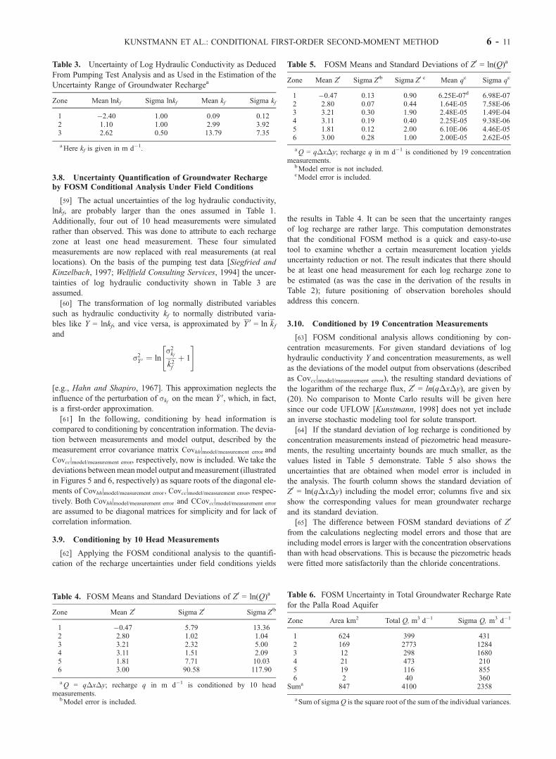
FOSM method, as it is presented in this work, was not performed.
[7] A modified approach of the FOSM method, which com-
putes sensitivity matrices by the repeated evaluation of the systemCopyright 2002 by the American Geophysical Union.0043-1397/02/2000WR000022$09.00
6 - 1
WATER RESOURCES RESEARCH, VOL. 38, NO. 4, 1035, 10.1029/2000WR000022, 2002
equation, was applied to a few field studies. James and Old-
enburg [1997] used the FOSM method to describe a trichlor-
ethylene contamination. Tiedemann and Gorelick [1993] applied
it to the optimization of a groundwater contaminant capture
design.
[8] Besides the FOSM method another numerical approach has
been used to treat stochastic groundwater flow: The distributed
parameter approach (DPA) is based on the differential equations
describing the mean and covariance of head. This approach has
been developed in detail by McLaughlin and Wood [1988] and was
explored in earlier work by Tang and Pinder [1977] and Devary
and Doctor [1982]. Graham and McLaughlin [1989a, 1989b] used
the DPA to derive expressions for predicting uncertainty in a solute
transport exercise and compared the results to Monte Carlo
analysis. The FOSM and the DPA are based on different Taylor
series approximations; however, the expansion is made around the
same set of variables. With FOSM the piezometric head (or solute
concentration matrix) is expanded around the model parameters
and substituted into the definition for the head (or solute concen-
tration) covariance matrix, whereas DPA is based on approximat-
ing matrix terms in a spatially discretized model system of
equations, perturbed around the model parameters. The second
difference is the manner in which the temporal discretization is
made. For DPA the temporal discretization is made on the head
covariance equation, whereas with FOSM a temporally discretized
Taylor series of the head equation is substituted into the head
covariance [Kunstmann, 1998]. At steady state the two methods
DPA and FOSM yield the same expression for the head covariance
matrix. The transient expressions for the head covariance matrices
differ, while the transient expressions for the cross-covariance
matrices (between heads and parameters) are found to be identical
[Connell, 1995; Kunstmann, 1998]. Another important difference
between the DPA and the FOSM approach, as presented in this
work, is that the FOSM method calculates the uncertainty prop-
agation for the coupled flow and transport equation. First, the
covariance matrix of the piezometric heads and the mixed param-
eter head covariance matrices are calculated by the uncertainty
propagation based on the flow equation. These three covariance
matrices, in turn, are prerequisites for the calculation of the
covariance matrix of the solute concentration. The requirements
of smallness of parameter variability are the same for both methods
as they are both linear. Other early papers [e.g., Delhomme, 1979;
Clifton and Neumann, 1982; Cooley, 1979] have addressed the
estimation of the covariance of predicted heads due to uncertain
parameters using other techniques. The application of derived head
statistics to Bayesian estimation is discussed, for example, by
Hoeksema and Kitanidis [1985] and Dagan [1982].
[9] If the probability associated with a limited number of
‘‘failure’’ states is of interest, the first-order reliability method
(FORM) can be used as a computationally efficient alternative to
Monte Carlo simulations. Such questions arise in the context of
safety assessments, where the probability of exceeding a target risk
level or a corresponding concentration threshold has to be deter-
mined. In FORM the exceedance probability is approximated to
first order. The FORM method was originally developed in the
field of structural reliability [Ang and Tang, 1984; Madsen et al.,
1986] and has been applied for uncertainty analyses of environ-
mental flow and transport problems since [Sitar et al., 1987;
Hamed et al., 1995; Xiang and Mishra, 1997; Skaggs and Barry,
1997].
[10] In this paper, the FOSM method is presented in a way
that is suitable for field case applications. The FOSM is embed-
ded in a finite difference approach and applied to both the partial
differential equations of groundwater flow and solute transport.
We extend the method to conditional analysis, showing how the
introduction of measurements of piezometric heads or solute
concentrations influence the uncertainty propagation. Closed
formulae obtained by the method clearly explain how condition-
ing information diminishes the uncertainty of model output.
These formulae quantify the uncertainty arising from the non-
uniqueness of the inverse problem. This ‘‘principle of interde-
pendent uncertainty’’ shows how the uncertainties of hydraulic
conductivity (or transmissivity) and groundwater recharge are
related to each other in the presence of head or concentration
measurements. The influence of model and measurement errors is
included. The proposed method is applied to a case study in
semiarid Botswana where the quantification of groundwater
recharge and its uncertainty bounds were of prime interest.
FOSM results are compared to results from a Monte Carlo
calculation.
[11] For a further example of the FOSM method the reader is
referred to Kunstmann and Kinzelbach [2000], who show the
application of the unconditional and conditional FOSM method
to the computation of stochastic wellhead protection zones for an
aquifer in Gambach (Germany) by combining the FOSM method
and Kolmogorov backward equation analysis. In contrast to
Kunstmann and Kinzelbach [2000] this paper introduces the theory
of unconditional and conditional FOSM method in detail as well as
the incorporation of model/measurement error.
2. Theory
2.1. The FOSM Method: Unconditional Moments
[12] The numerical solution of the two-dimensional steady state
groundwater flow equation for confined aquifers
r � mkfrh� �
þ q ¼ 0 ð1Þ
is usually obtained by finite element or finite difference schemes
for unknown piezometric head h at specified grid points,
represented as a vector h. The aquifer parameters, such as the
hydraulic conductivity kf (length time �1), the thickness of the
aquifer m (length), and the recharge/discharge rates q (length3
time �1 length �2) can also be specified as vectors p at all grid
points.
[13] In subsurface hydrology, flow parameters such as hydraulic
conductivity are often found to be lognormally distributed in space
[Gelhar, 1993]. In the following it is assumed that both the
hydraulic conductivity kf and the groundwater recharge q are
lognormally distributed. Thus Y = ln kf and Z = ln q are normally
distributed stochastic variables. Whereas the assumption of a
lognormally distributed hydraulic conductivity is experimentally
well justified [e.g., Gelhar, 1993], a lognormally distributed
groundwater recharge, however, is assumed for purely practical
reasons: When applying parameter estimation algorithms, as per-
formed in the application presented in this work, positive values for
groundwater recharge are always obtained. The assumption of
lognormally distributed kf and q is not a restriction to the general-
ity of the method. Everything could be also derived for quantities q
and kf instead of Y and Z. The aquifer parameters p (i.e., log
hydraulic conductivity Y or log recharge Z ) are assumed to be
uncertain. They are described under the preceding assumptions as
having a mean value p and a covariance Cov (p). If the model
setup is based on a zonation of log hydraulic conductivity, the
elements of Y are given by zonal values of Y : Y 2 <NY, with <
6 - 2 KUNSTMANN ET AL.: CONDITIONAL FIRST-ORDER SECOND-MOMENT METHOD

indicating the space of real numbers and with NY equal to the
number of zones within which log hydraulic conductivity Y is
assumed to be uniform. The same can hold for Z. If the zonal
values are uncorrelated, CovYY , and CovZZ are of diagonal shape.
The entries of the diagonal elements are the squared standard
deviations of the uncertainties of the zonal values.
[14] The first moment of the heads is approximated to first-order
accuracy [Dettinger and Wilson, 1981] by the mean heads h
obtained as the solution of (1) using the mean values of the aquifer
parameters p.
E h pð Þ½ � ¼ h¼1 h pð Þ: ð2Þ
The propagation of parameter uncertainties into the head
uncertainties, given by the covariance matrix Cov(h), can be
approximated by inserting the Taylor series expansion of h into
Covhh � Cov hð Þ ¼ E h� h� �
� h� h� �� �
; ð3Þ
yielding
Covhh ¼1DhY � CovYY � DT
hY þ DhZ � CovZZ � DThZ
þ DhZ � CovZY � DThY þ DhY � CovYZ � DT
hZ ; ð4Þ
where the superscript T denotes the transpose of the matrix. The
parameter head cross-covariance matrices are obtained from
CovhY � E h� h� �
� Y� Y� �� �
¼1 DhY � CovYY þ DhZ � CovZY ð5Þ
CovhZ � E h� h� �
� Z� Z� �� �
¼1 DhZ � CovZZ þ DhY � CovYZ ð6Þ
[Dettinger and Wilson, 1981; Townley and Wilson, 1985]. The
superscript above the equal sign indicates the order of the approx-
imation. DhY � DYThð ÞjY¼ Y; Z¼ Z
andDhZ � DZT hð ÞjY¼ Y; Z¼ Z
are
first derivatives of h with respect to the transpose of the parameter
vectors (Y, Z), evaluated at their mean values. These derivatives
are Jacobian matrices expressing the sensitivity of hi to variations
or uncertainties in Yj and Zj. In unconditional analysis it is
assumed that Z and Y are uncorrelated and that CovYZ = CovYZ =
null matrix. Since the second moments are calculated in first-order
accuracy, the method is named the ‘‘first-order second-moment
method.’’
[15] The FOSM method is now applied to the two-dimensional
(2-D) steady state solute transport equation [e.g., Bear, 1972]
nm r � vcð Þ � r � Dmol þ Ddisp
� �� rc
�� �� qcin ¼ 0;
�ð7Þ
where c is solute concentration (mass length�3 ), v is 2-D pore
velocity vector (length time�1), nm is mobile porosity [dimen-
sionless], Dmol is molecular diffusion coefficient (length2 time�1),
Ddisp is dispersion tensor (length2 time�1) according to
[Scheidegger, 1961], q is recharge per unit horizontal area
(length3 time�1 length�2), cin is pollutant concentration in
inflows to aquifer (mass length�3), and m is thickness of aquifer
(length).
[16] The velocity v is given by Darcy’s law:
v ¼ � 1
nmkfrh ¼ � 1
nmeYrh: ð8Þ
The first-order approximation of the mean concentrations E(c) is
the solution of the partial differential equation using the mean
values of all aquifer parameters,
E c Y;Z; hð Þ½ � ¼ c¼1 c Y; Z; h� �
: ð9Þ
The covariance of the concentration in steady state can be derived
in analogy to the flow equation and is given by
Covcc ¼1Dch � Covhh � DT
ch þ DcY � CovYY � DTcY þ DcZ � CovZZ � DT
cZ
þ Dch � CovhY � DTcY þ DcY � CovYh � DT
ch
þ Dch � CovhZ � DTcZ þ DcZ � CovZh � DT
ch
þ DcY � CovYZ � DTcZ þ DcZ � CovZY � DT
cY : ð10Þ
Dch, DcY, and DcZ indicate the sensitivity matrices of the solute
concentration with respect to the piezometric heads, log
hydraulic conductivity Y, and log recharge Z. The computation
of Covcc requires evaluation of Covhh, CovhY, and CovhZ from
(4), (5), and (6). The uncertainty of the concentrations is then
described in terms of variances of c, given by sc2, the diagonal
elements of Covcc.
[17] The computational advantage of the FOSM method
depends on how the sensitivity matrices are calculated and how
matrix multiplications are organized. Details are given by Kunst-
mann [1998]. Thus the rank of the n � n covariance matrices, such
as Covhh and Covcc, is the limiting factor for the computational
efficiency of the method. If only the variances of the head
simulations are of interest, calculation of the diagonal of Covhhis sufficient. However, if the uncertainties of the solute concen-
trations are required, all entries of Covhh must be evaluated. In the
application presented in section 3, only the standard deviations of
the concentrations are of interest, and thus only the diagonal
elements of Covcc need to be calculated. If only specific grid
points are of interest, one can skip the computation for other grid
points thus reducing computational effort.
[18] Uncertainty in the dispersion tensor Ddisp implicitly is
included in the analysis as far as it can be traced back to uncertainty
in the velocity field. Uncertainty in the velocity field, in general,
arises from uncertainty in hydraulic conductivity, piezometric
heads, thickness of the aquifer, and porosity (equation (8)). The
uncertainty in conductivity and recharge propagates into uncer-
tainty in heads, which, in turn, propagates into uncertainty in the
velocity field. Porosity and the thickness of the aquifer are assumed
to be known ‘‘perfectly.’’ The same holds for dispersivity, which
together with the velocity field, constitutes Ddisp. In principle, there
is no difficulty extending the FOSM approach to additional uncer-
tainties such as uncertainty of porosity, thickness of the aquifer, or
dispersivities.
[19] In the unconditional case presented so far, the mixed
parameter covariances, CovZY and CovYZ, are assumed to vanish;
that is, the uncertainties of log recharge and log hydraulic
conductivity are assumed to be uncorrelated. In the presence
of head or concentration measurements these uncertainties
become related to each other as the measurements express the
interaction of both. This relationship leads to the conditional
FOSM method.
2.2. FOSM Method: Conditional Moments
[20] Usually, estimates of hydraulic conductivity and recharge
are obtained by inverse modeling techniques. In a steady state
KUNSTMANN ET AL.: CONDITIONAL FIRST-ORDER SECOND-MOMENT METHOD 6 - 3
calibration process, aquifer parameters are varied until measured
and simulated heads at the observation points agree as closely as
possible, for example, until
c2 ¼XNi¼1
hmodeled;i � hobserved;i� �2
s2hobserved;i! min ) Y ; Z; ð11Þ
with Y and Z being the corresponding optimal parameter estimates.
Unfortunately, this calibration can lead to nonunique results [e.g.,
Carrera and Neumann, 1986], as different sets of parameters Y
and Z can yield the same distribution of simulated piezometric
heads, especially if both fluxes and hydraulic conductivities are
unknown. For example, for negligible well discharge, essentially
the same head distribution can be obtained for high recharge and
high hydraulic conductivity, as well as for low recharge and low
hydraulic conductivity. In general, there is a set of combinations of
Y and Z that lead to a practically identical model output at the
measurement locations. A decisive question of parameter estima-
tion therefore is which set of recharge rates Z 2 Z � sZ� �
will
lead to an identical model output at the measurement locations for
a given set of possible hydraulic conductivities Y 2 Y � sY� �
.
[21] A ‘‘principle of interdependent uncertainty’’ can be derived
from the equations of the unconditional FOSM method using the
idea that, if specific entries of Covhh or Covcc are known through
measurements, the uncertainty propagation equations yield non-
trivial correlations between the parameter covariances CovZZ and
CovYY. The measurement of a piezometric head at grid point
location k gives knowledge of that head within its uncertainty
bounds because of measurement errors. Its uncertainty, shk , is
therefore reduced to the measurement error sh|measurement error. All
covariance matrix elements composed of factors, shk , such as
Covhh, CovhY, and CovhZ, then read (with r indicating the
correlation coefficient) as follows:
Covhh k;l
�� ¼ rhkhlshkshl ð12Þ
if k or l are measurement locations,
CovhY k;i
�� ¼ rhkYishksYi ¼ 0; 8i ¼ 1; . . . ;NY ð13Þ
if k is the measurement location,
CovhZ k;j
�� ¼ rhkZjshksZj ¼ 0; 8j ¼ 1; . . . ;NZ ð14Þ
if k is measurement location. In the example presented, it is
assumed that there is no correlation between measurement errors of
heads and parameters Y and Z. Therefore (12) reduces toCovhh k;k
�� ¼ s2hk . Equations (12)–(14) determine the relationship
between uncertainties in Y and Z when heads are used for
conditioning.
[22] To establish the system of equations that determines the
relation between CovYY and CovZZ, the n � n head covariance
matrix Covhh is projected to a Nh � Nh ‘‘measurement subspace,’’
where Nh is the number of head measurements. The projection
matrix P has Nh rows and n columns:
P 2 <Nh�n ð15Þ
The rows of P are unit vectors e 2 <n with ei = 1 if i is a
measurement location. By defining ~Dhy = PDhY, and ~DhZ = PDhZ,
one obtains the requirement
Cov0hh � P Covhh PT ¼ ~DhY CovYY ~DT
hY þ ~DhZ CovZZ ~DThZ
þ~DhZ CovZY ~DThY þ ~DhY CovYZ ~DT
hZ
¼! Cov0hh measurement error;j ð16Þ
with Covhh|measurement error denoting the measurement error
covariance matrix. If the errors are not correlated, this matrix is
of diagonal form. In practical applications one can interpret the
deviations between model output and measurement values as a
combined model and measurement error sh. It is in this way that a
‘‘goodness of fit’’ criterion enters the conditional first-order
second-moment method.
[23] Equation (16) can be solved exactly for CovZZ if the
number of head measurements Nh is equal to the number of
parameters whose uncertainty range is to be estimated. If Nh is
greater than NZ, the system is overdetermined, and (16) can only be
fulfilled in a least squares sense. In that case, CovZZ must be
determined in a way such that kCov0hh – Covhh|measurement errork2 isminimal (where k k2 denotes the square norm of a matrix):
Cov0hh � Covhh jmeasurement error
2! min: ð17Þ
If the uncertainty range of log recharge Z is of interest, (16) can be
solved for CovZZ:
CovZZ ¼ ~DThZ � ~DhZ
� ��1� ~DThZ � ðCovhhjmeasurement error � ~DhY � CovYY
� ~DThY � ~DhZ � CovZY � ~DT
hY � ~DhY � CovYZ � ~DThZÞ
� ~DhZ � ~DThZ � ~DhZ
� ��1: ð18Þ
The residual of (17) is then minimal, because CovZZ is obtained by
solving the normal equations of a regression problem [Golub and
Van Loan, 1996]. In case there are less head measurements than
zones, that is, the model is overparameterized, the system of
equations is undetermined, and no regression is possible.
[24] The expression for CovZY in (18) can be derived by (13)
and (5), finally leading to
CovZY ¼ � ~DThZ � ~DhZ
� ��1� ~DThZ
~DhY � CovYY : ð19Þ
For each value of log hydraulic conductivity Y that lies within its
certainty range (given by the trace CovYY), there will be a value of
log recharge Z within its uncertainty range (given by the trace
CovZZ) that ensures that the model output at the measurement
points will remain the same. Equation (18) quantifies this
interdependence of the uncertainty ranges of log transmissivity Y
and log recharge Z. This is the principle of interdependent
uncertainty.
[25] Similarly to the derivation of CovZZ, the uncertainty range
of log hydraulic conductivity Y, CovYY, at given CovZZ can be
derived. Concentration measurements can likewise be used in
conditioning the uncertainty range of either CovZZ or CovYY.
Similarly to the relation between CovZZ and CovZY for given head
measurements, relations on the basis of concentration measure-
ments can be deduced. The uncertainty range of log recharge Z for
given concentration measurements and uncertainty in log trans-
missivity Y can be evaluated as
CovZZ ¼ ~DcZ þ ~Dch � DhZ
� �T � ~DcZ þ ~Dch � DhZ
� �h i�1
� ~DcZ þ ~Dch
�� DhZÞT � Covcc measurement errorj � ~DcY � CovYY � ~DT
cY
�
6 - 4 KUNSTMANN ET AL.: CONDITIONAL FIRST-ORDER SECOND-MOMENT METHOD
�~DcY � CovYZ � ~DTcZ � ~DcZ � CovZY � ~DT
cY
�~Dch � DhYCovYY � DThY � ~DT
ch � ~Dch � DhZCovZY � DThY � ~DT
ch
�~Dch � DhY � CovYZ � DThZ � ~DT
ch
�~DcY � CovYh � ~DTch � ~Dch � CovhY � ~DT
cY
�~DcZ � CovZY � DThY � ~DT
ch � ~Dch � DhY � CovYZ� ~DT
cZ
�� ~DcZ þ ~Dch � DhZ
� �� ½ð~DcZ þ ~Dch � DhZÞT
� ð~DcZ þ ~Dch � DhZÞ��1; ð20Þ
with CovZY given by
CovZY ¼ � ~DcZ þ ~Dch � DhZ
� �T � ~DcZ þ ~Dch � DhZ
� �h i�1
� ~DcZ þ ~Dch � DhZ
� �T ~DcY þ ~Dch � DhY
� �CovYY : ð21Þ
Equations (20) and (21) again relate the covariances of CovYY and
CovZZ to each other, now expressing the principle of interdepen-
dent uncertainty in the presence of concentration measurements.
[26] In the Monte Carlo approach, the primary alternative to this
approach, the incorporation of head or concentration information is
much more tedious and costly: A conditional Monte Carlo simu-
lation requires the application of the inverse method for each
realization.
[27] The deviations between measured and computed values are
not only due to measurement error but also to the inadequacy of
the model. To the latter type of error, which arises, for example,
from the limited validity of equations applied, the limited reso-
lution of input parameters, or two-dimensional flow and transport
approximation, we refer to as ‘‘model error’’ in this work. Every-
thing said above about measurement error can therefore be
extended to model error. Since the model error could be spatially
correlated, Covhh|measurement/model error would be a full matrix.
2.3. Limitations of the Method
[28] The FOSM method has two main limitations. First, the size
of the covariance matrices can become infeasibly large as the
number of nodes in the model becomes large. Owing to this
limitation, realistic calculations are at present confined to steady
state models of flow and transport. In time varying computations
the large n � n matrices Covhh and Covcc have to be propagated at
each time step, diminishing the computational efficiency relative to
alternatives such as the Monte Carlo method. The limitation to
steady state situations for piezometric heads and solute concen-
trations restricts the range of applications for which the FOSM
method in its presented formulation can be used. However,
important tasks remain where this limitation does not matter.
One is the application of the FOSM method to the determination
of stochastic wellhead protection zones [Kunstmann et al., 1998;
Kunstmann, 1998]. Another feasible application is the estimation
of the uncertainty range of aquifer parameters such as groundwater
recharge by conditioning with steady state environmental tracer
data, as described in this paper.
[29] Second, uncertainty in parameters must be moderate, as the
method is inherently a linear method.
[30] The first limit can partly be overcome by the efficient
multiplication of matrices. At present, the number of nodes can be
as much as several thousand nodes, which is sufficient for two-
dimensional case studies.
[31] An extension of the Taylor series expansion to second-
order terms, in principle, can improve the restriction on the limited
variability of aquifer parameters. Such an extension yields the
second-order second-moment method. The computationally effi-
cient calculation of second derivatives, however, is cumbersome to
realize in a computer code.
3. Application
3.1. Background
[32] The conditional FOSM method is now applied to an aquifer
in semiarid Botswana. The code UFLOW [Kunstmann, 1998]
contains all relevant routines of the theory presented and addition-
ally the algorithms for the corresponding Monte Carlo simulations.
This allows the comparison of the conditional FOSM method with
inverse stochastic modeling by Monte Carlo simulations.
[33] The future water supply of Gaborone, the capital of
Botswana, is to be ensured by the construction of the North-South
Water Carrier. Once finished, water will be collected in a dam in
the northeastern part of the country and transported over �300 km
to the city by means of a pipeline. If the system fails, either because
of lack of water in the dam or technical problems with the pumping
system, backup solutions based on groundwater resources are
required. Several aquifers between Gaborone and Francistown
have been investigated in terms of their potential yields. The
groundwater abstraction potential of the Ntane sandstone aquifer
in the Palla Road area (see Figure 1) is considered here [see also
Siegfried and Kinzelbach, 1997]. Sustainability in the context of
groundwater resources management requires that extractions from
the aquifer do not exceed natural replenishment over a prolonged
time period. The concept allows overdraft if a recovery period is
subsequently granted to meet the equilibrium condition in the long
run. Since the recharge rate is of major importance for the long-
term extraction capacity, sustainable groundwater management
requires quantification of its uncertainty bounds:
qrecharge
¼ qrecharge
� srecharge
ð22Þ
or, if the recharge is assumed to be lognormally distributed, with
Z = ln qrecharge,
Z ¼ Z � sZ : ð23Þ
Once the uncertainty bounds of qrecharge are quantified, con-
servative and sustainable decisions can be made.
3.2. Hydrogeological Setting of the Palla Road Aquifer
[34] Kalahari beds of variable thickness (up to 40 m) cover the
model area and together with the several underlying layers described
below constitute the Palla Road Aquifer. These deposits tend to
thicken toward the center of the Kalahari basin situated to the west.
They consist of unconsolidated aeolian sands, which commonly are
calcretized or silcretized. In areas with extensive calcretization, such
as pan structures, total dissolved solids (TDS) measurements of
shallow groundwater confirm that substantial groundwater replen-
ishment (i.e., >1 mm yr�1) is restricted to areas with little calcreti-
zation [Moehadu, 1997]. Below the Kalahari beds a basalt layer of
variable thickness extends under �75% of the area. The variability
of the thickness is related to intensive faulting as well as to the
unevenness of the topography on which the lava was extruded. The
basalt cover tends to thicken toward the west. Groundwater recharge
potential increases where the basalt layer is thinner and where the
basalt is fractured. The underlying Lebung formation consists of an
aquitard (Mosolotsane siltstones) and the Ntane sandstone aquifer.
The Mosolotsane siltstone shows a gradual transition into the
predominantly sandy Ntane, which occasionally contains lenses of
KUNSTMANN ET AL.: CONDITIONAL FIRST-ORDER SECOND-MOMENT METHOD 6 - 5

siltstone. The Mosolotsane siltstone formation acts as a hydraulic
boundary between the underlying highly saline Ecca sandstone
aquifer and the Ntane freshwater aquifer. However, there are
locations where the Ecca sandstone is shifted against the Ntane
sandstone or where a hydraulic connection between the two aquifers
is established because of a structural weakness of the Mosolotsane
formation. In these locations, contamination of Ntane water with the
saline Eccawaters occurs. Transport modeling of TDS concentration
will address this concern. The Ntane sandstone outcrops between the
Palla Road wellfield (in the southeastern quadrant of the model grid,
see Figure 2) and the Kadimotse fault where the basalt cover is
missing (�25% of the model area). The excellent water quality
found in the Palla Road wellfield is related to a strongly increased
recharge in this outcrop area.
[35] Estimates of mean recharge values were made using the
soil chloride method [Gieske, 1992], which was first introduced by
Figure 1. Site location of the Palla Road Aquifer.
Figure 2. Six recharge and lateral inflow zones of the Palla Road Aquifer with log recharge q in ln(m d�1) werechosen. Fixed-head cells are indicated also.
6 - 6 KUNSTMANN ET AL.: CONDITIONAL FIRST-ORDER SECOND-MOMENT METHOD
Eriksson and Khunakasem [1969]. Evaporation and recharge rates
are estimated by determining the ratio of average chloride content
in precipitation to that in groundwater. This technique has been
used to evaluate recharge in a range of environments [Allison and
Hughes, 1978; Edmunds and Walton, 1980; Sharma and Hughes,
1985; Gieske, 1992; Wood and Sanford, 1995]. Reviews of the
method are given by Simmers [1988] and Lerner et al. [1990].
3.3. Model Layout and Boundary Conditionsfor the Palla Road Aquifer
[36] The model area extends over 57 km in the east-west
direction and 34 km from northeast to southeast. The total head
difference over the length of the aquifer is �100 m. The spatial
discretization lengths�x and�y were chosen as 1000 m [Siegfried
and Kinzelbach, 1997]. The aquifer was assumed to be confined
with aquifer thickness estimated from borehole logs [Wellfield
Consulting Services, 1994]. Longitudinal dispersivity aL was
estimated to be 1 km, and transversal dispersivity aT was set to
100 m.
[37] The recharge pattern was divided into six different zones.
These groundwater recharge zones are assumed to represent areas
with uniform recharge rates, with values that are uncertain and
have a lognormal distribution. In the following the six zones of log
recharge Z are summarized in the log recharge vector Z 2 <6. The
recharge zonation and the locations of the lateral inflows and their
corresponding values are shown in Figure 2. Zone 1 covers the
largest part of the model region and encompasses the area where
the Ntane sandstone is covered with Stromberg lava. Recharge is
highest in the Ntane sandstone outcrop areas (zone 2, in the
northeast of the model area). Boundary fluxes were estimated from
the area of the catchments draining into each boundary segment
using areal recharge rates from information provided by Wellfield
Consulting Services [1994].
[38] Zone 4 accounts for the contamination of the Ntane water by
groundwater originating from the Ecca aquifer (Ecca-Saltwater
Intrusion). Assuming proportionality between chloride and TDS
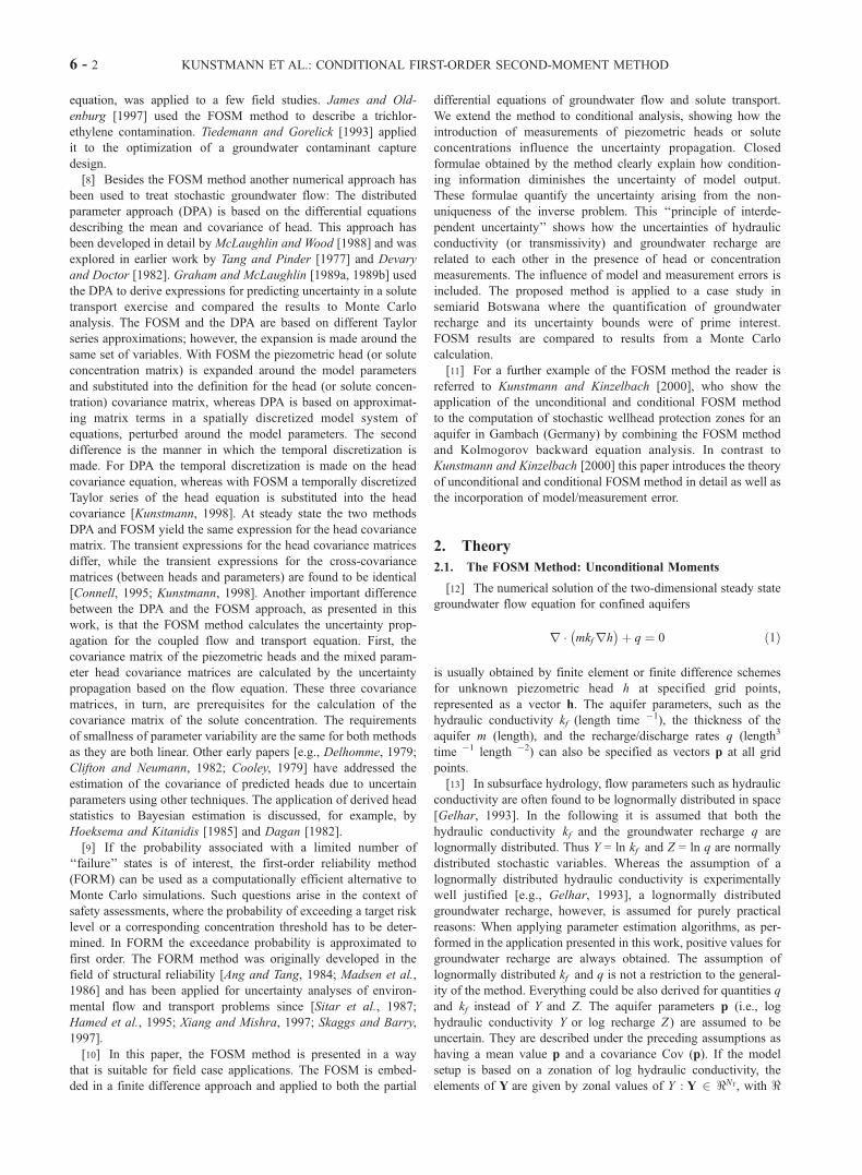
concentration, the TDS concentrations of inflows shown in Figure 3
can be estimated using the soil chloride method [see Siegfried and
Kinzelbach, 1997].
[39] The only outflow from the model area is on the southeastern
edge. It was modeled by a fixed-head boundary (see Figure 2), since
in the prepumping steady state situation the boundary always was
on outflow boundary.
[40] Siegfried and Kinzelbach [1997] developed a deterministic
flow and transport model adjusting the hydraulic conductivities
such that simulated heads and chloride concentrations matched
observations, assuming that recharge data were more reliable than
conductivity data. Recharge estimates could be justified by both
flow and salinity conditions, while the conductivities were only
known as point values from pumping test sites, which are not
representative of mean values for the zones used. Steady state
calibration attempted to match observed heads in 1992, the first
year with sufficient data. A cone of depression resulting from
groundwater extraction in the Palla Road wellfield had at that time
not yet spread, and extraction could be neglected. The hydraulic
conductivity distribution was divided into three zones, based on
geological structures following fault lines and a paleochannel
structure along the centerline of the aquifer. The model parameter
values were calibrated by taking into account both piezometric
head and TDS concentration measurements.
[41] The calibrated zones of log hydraulic conductivity Y0 = ln kf,
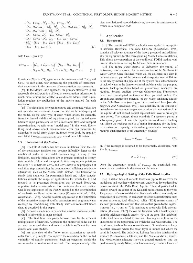
with zonal parameters, are shown in Figure 4. In the following the
three zones of log hydraulic conductivity Y are summarized in the
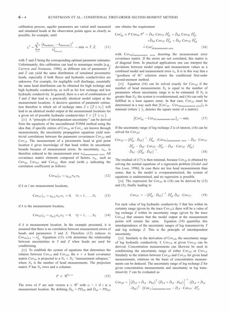
vector Y0 2 <3. On the basis of these mean parameters, flow and
solute transport can be simulated. The good correspondences
between observed and calculated heads and concentrations are
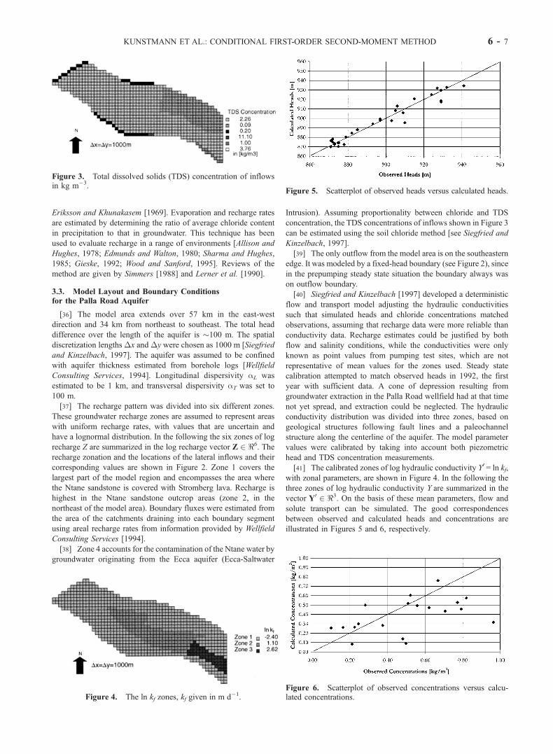
illustrated in Figures 5 and 6, respectively.
Figure 3. Total dissolved solids (TDS) concentration of inflowsin kg m�3.
Figure 4. The ln kf zones, kf given in m d�1.
Figure 5. Scatterplot of observed heads versus calculated heads.
Figure 6. Scatterplot of observed concentrations versus calcu-lated concentrations.
KUNSTMANN ET AL.: CONDITIONAL FIRST-ORDER SECOND-MOMENT METHOD 6 - 7

[42] The correlation between observed and calculated concen-
trations is less satisfactory than for heads. The deviations are due to
the simplification of the natural system by choosing a two-dimen-
sional model with a very limited number of free parameters.
Calculations yield an integral value over the whole depth not
accounting for the actual salinity profile. Little knowledge on the
situation at the boundary is available. Also, salinity intrusion from
the Ecca aquifer into some boreholes may be contaminating some
observations [Siegfried and Kinzelbach, 1997].
[43] The fitted values of hydraulic conductivity kf and the
assumed values for groundwater recharge q are only one set of
parameters that can satisfy observed head and concentration
measurements. In terms of the sustainability constraint it is there-
fore vital to quantify the uncertainty range of groundwater recharge
associated with the nonuniqueness of the solution of the inverse
problem as well as with the quality of the data.
3.4. Corresponding Monte Carlo Simulation
[44] In the following the conditional FOSM method is
compared to inverse stochastic modeling by conditional Monte
Carlo simulations. The comparisons, for simplicity, will first
assume that there are no model and measurement errors (i.e.,
Covhh|model/measurement error = null matrix). The uncertainty of the
log hydraulic conductivity, as estimated by pumping test anal-
ysis, is used to deduce the FOSM interdependent uncertainty of
log recharge Z, according to (18), and (20). Section 3.5
describes how a Monte Carlo simulation is performed that
corresponds to the conditional FOSM method so that a compar-
ison of the two methods is possible.
[45] A conditional Monte Carlo simulation generates realiza-
tions of log hydraulic conductivity according to an assumed
covariance structure. Then, for each log hydraulic conductivity
realization the parameters of log recharge are fitted such that the
weighted least squares deviation c2 between measured and mod-
eled values of piezometric heads is minimized. The example
discussed assumes that the uncertainties of the three zones of
hydraulic conductivity are uncorrelated; the matrix CovYY is there-
fore diagonal. Random realizations of log hydraulic conductivity Y
can be generated by Cholesky decomposition [Press et al., 1992]
of the covariance matrix CovYY, following Robin et al. [1993], for
any given covariance structure. Details are given by [Kunstmann,
1998]. When CovYY is diagonal, the decomposition is trivial.
[46] For each realization v of log hydraulic conductivity Y the
flow model must be run in inverse mode to fit the corresponding
log recharges Z,
vYrandom;v c2 ¼
XNi¼1
hmodeled;i � hobserved;i� �2
s2hi! min;
)v Zestimated: ð24Þ
This minimization was accomplished here by application of the
Marquardt-Levenberg algorithm [Press et al., 1992] to each
realization of Y. Convergence of first and second moments of
concentrations in the Monte Carlo approach is checked by
monitoring the evolution of the average-per-node (APN) first and
second moment of TDS concentration as N 0MC is increased:
cAPN N 0MC
� �¼ 1
n
Xj;iegrid
c j;i N0MC
� �ð25Þ
s2cAPN N 0MC
� �¼ 1
n
Xj;iegrid
s2c j;iN 0MC
� �: ð26Þ
N0MC denotes the number of Monte Carlo realizations performed at
which (25) and (26) are evaluated; n denotes the total number of
nodes. In addition, the mean and the variance of the zonal values of
the generated log hydraulic conductivity Y and the fitted log
recharge Z are calculated.
[47] In steady state situations (as in the case study discussed) the
Marquardt-Levenberg algorithm requires estimates of the sensitiv-
ities @h/@p; in this application the sensitivities were determined by
direct derivation from the model equations (see Kunstmann [1998]
for details). If the parameters to be estimated are the log recharge Z,
the sensitivities required by the Marquardt-Levenberg algorithm
are the entries of the sensitivity matrix DhZ
@hmodeled;i
@Zk¼ DhZ l¼i;k
�� ð27Þ
introduced in (4), (5), and (6). The CPU time savings by the direct
evaluation of these sensitivities are enormous. The conditional
Monte Carlo method used in this study is therefore already
computationally more efficient than one based on sensitivity
calculations that use a secant approximation [Yeh, 1986]. Never-
theless, the conditional Monte Carlo method is still computation-
ally more demanding than the conditional FOSM method, as
shown in section 3.5.
3.5. Comparison Between Conditional FOSM Methodand Conditional Monte Carlo Simulation
[48] In the following analysis, Z0 = lnQ = ln(q�x�y) is used as
the variable describing recharge instead of Z = lnq. With given
head measurements and for a given level of uncertainty in log
hydraulic conductivity Y (Table 1), the conditional FOSM method
first calculates the mixed covariances CovZ0Y and CovYZ0 (equation
(19)) and then the uncertainty of Z0, expressed through its cova-
riance matrix CovZ0Z0 (equation (18)). These uncertainties then are
propagated into estimates of piezometric head and solute concen-
tration uncertainty (equations (4) and (10)).
[49] For the purpose of investigating the equivalence between the
FOSM and Monte Carlo methods the uncertainty range of Y = lnkf is
chosen such that the first-order approximation of the FOSMmethod
is valid. Ten head measurements were selected for the inverse
stochastic analysis of the Palla Road Aquifer. Four out of the 10
were interpolated since there was not a measurement available in
each zone of groundwater recharge. The four synthetic head
measurements will be replaced by real head measurements, and a
larger CovYY will be used in section 3.6.
[50] Our assumption of no model and measurement errors
means that the fitting of recharge values for each realization of
the Monte Carlo simulation is performed with the head values
calculated by the mean model parameters, Y and Z0, instead of the
real head measurements. This approach is necessary to be fully
compatible with the conditional FOSM method in the formulation
that does not include model and measurement errors. The deviation
Table 1. Mean and Standard Deviation of lnkf for the Three
Hydraulic Conductivity Zones as Used in the Comparison Between
Conditional FOSM Method and Conditional Monte Carlo Methoda
Zone Mean lnkf Sigma lnkf Mean kf Sigma kf
1 �2.40 0.40 0.09 0.042 1.10 0.40 2.99 1.253 2.62 0.20 13.79 2.79
aHere kf is given in m d�1.
6 - 8 KUNSTMANN ET AL.: CONDITIONAL FIRST-ORDER SECOND-MOMENT METHOD

of measured heads from the average computed heads is for our
purposes primarily the model error that will be discussed in section
3.8 and section 3.9.
3.6. Comparison of Resulting CovZZ Between FOSMand Monte Carlo Method
[51] As a check of the conditional FOSM method and the
principle of interdependent uncertainty, we first compare the
diagonal of CovZ0Z0 obtained by (18) with Monte Carlo statis-
tics. FOSM conditional analysis gives the uncertainty of log
recharge CovZ0Z0 for specified head measurements and specified
CovYY.
[52] The square roots of the diagonal elements of CovZ0Z0 from
FOSM are compared to the log recharge rates fitted in the condi-
tional Monte Carlo simulations in Table 2. The good correspond-
ence between Monte Carlo and FOSMmethod results clearly shows
the consistency of the proposed FOSM formulae. The calculated
CovZ0Z0 is now inserted into the propagation of the head and
concentration uncertainty, and the results are compared to the
Monte Carlo method. The calculation of the covariance propagation
of Covhh and Covcc is performed according to the expressions given
in (4) and (10).
3.7. Comparison of First and Second Moments of Headsand TDS Concentrations
[53] The resulting mean piezometric head distribution is illus-
trated in Figure 7. Increased recharge is responsible for the steep
gradients visible in the northeastern area, whereas higher effective
conductivity in the graben structure to the south diminishes head
gradients there. There is no difference in the results between
FOSM and Monte Carlo approach, indicating that the first moment
is not yet influenced by the parameter perturbation.
[54] The second moment of the piezometric head is illustrated in
Figures 8 and 9. The first and second moments of heads from the
FOSM and Monte Carlo results are satisfactorily similar. There are
10 local minima for the standard deviation of the heads in fact,
exactly at the 10 measurement locations. These minima are
smoothed in Figures 8 and 9 because of the interpolation applied.
The minima would be exactly equal to zero if (16) could be solved
exactly, that is, if the number of head measurements would be equal
to the number of groundwater recharge zones. In the case of 10 head
measurements and six groundwater recharge zones, as in the
example presented, (16) can only be fulfilled in a least squares
sense, yielding local minima of the heads’ standard deviations at the
measurement locations.
[55] Figure 10 shows the concentration distribution. The calcu-
lation confirms that the excellent water quality found in the Palla
Road wellfield can be explained by the increased recharge in the
area where the Ntane sandstone outcrops. The intrusion of low-
quality water still represents the main threat to the Palla Road
wellfield and is visible as a saltwater plume along the southern
boundary of the aquifer. FOSM and Monte Carlo distributions of
mean concentrations correspond well, indicating that the first
moment of the TDS concentrations has also not been shifted by
the parameter uncertainties.
Table 2. Comparison of Mean Z 0 and Standard Deviation Sigma
Z0 as Calculated by the Monte Carlo and the FOSM Methodsa
Zone MONTE CARLO FOSM
Mean Z0 Sigma Z0 Mean Z0 Sigma Z0
1 �0.58 0.78 �0.47 1.212 2.77 0.30 2.80 0.353 3.13 0.32 3.21 0.594 3.03 0.26 3.11 0.225 1.73 0.29 1.81 0.326 2.76 0.81 3.00 0.98
aZ0 = ln(Q), Q = (q�x�y), and recharge q is given in m d�1.
Figure 7. First moment of heads in meters (first-order second-moment (FOSM) method, Palla Road Aquifer, conditioned by 10head measurements).
Figure 8. Standard deviations of heads in meters (FOSMmethod, Palla Road Aquifer, conditioned by 10 head measure-ments).
Figure 9. Standard deviations of heads in meters (Monte Carlomethod, Palla Road Aquifer, conditioned by 10 head measure-ments).
KUNSTMANN ET AL.: CONDITIONAL FIRST-ORDER SECOND-MOMENT METHOD 6 - 9

[56] Figures 11 and 12 show the standard deviations of TDS
concentrations, conditioned by the 10 head measurements. The
similarities between standard deviations from the FOSM method
and Monte Carlo method are clearly visible. The FOSM standard
deviation is larger in the southeastern region than in theMonte Carlo
result.
[57] The convergence behavior of the Monte Carlo simula-
tion, according to (25) and (26), is illustrated in Figure 13.
About 500 realizations were sufficient to achieve convergence.
Only 694 out of the 750 realizations of the Monte Carlo method
were accepted to be included into the statistics since the c2
values of the remaining 56 realizations exceeded the specified
threshold value. The FOSM method was �35 times less
demanding of CPU time than 500 Monte Carlo realizations
and was 60 times less demanding than 750 Monte Carlo
realizations. If the convergence control variables were normally
distributed, one could give a priori estimates for the required
number of Monte Carlo simulations for any desired confidence
levels [e.g., Bronstein et al., 1996].
[58] If one is only interested in the uncertainty range CovZ0Z0
(equation (18)) and not in the resulting uncertainty of the head or
concentration distribution, Covhh (see Figures 8 and 9) and Covcc(see Figures 11 and 12), the FOSM method shows its largest
advantage over the Monte Carlo method. In this case the prop-
agation of large size covariance matrices required for obtaining
Covhh and Covcc can be omitted in the FOSM method, whereas the
Monte Carlo method still requires the time-consuming repeated
solution of the system equations for the random realizations
generated. The CPU time requirement for the calculation of
standard deviations sz of the FOSM method alone (Table 2) is
<1% of the Monte Carlo requirements.
Figure 10. First moment of concentrations in kg m�3 (FOSMmethod, Palla Road Aquifer, conditioned by 10 head measure-ments).
Figure 11. Standard deviations of concentrations in kg m�3
(FOSM method, Palla Road Aquifer, conditioned by 10 headmeasurements).
Figure 12. Standard deviations of concentrations in kg m�3
(Monte Carlo method, Palla Road, conditioned by 10 headmeasurements).
Figure 13. Convergence behavior of (a) first and (b) secondmoment of concentrations (Monte Carlo method, Palla RoadAquifer, conditioned by 10 head measurements).
6 - 10 KUNSTMANN ET AL.: CONDITIONAL FIRST-ORDER SECOND-MOMENT METHOD
3.8. Uncertainty Quantification of Groundwater Rechargeby FOSM Conditional Analysis Under Field Conditions
[59] The actual uncertainties of the log hydraulic conductivity,
lnkf, are probably larger than the ones assumed in Table 1.
Additionally, four out of 10 head measurements were simulated
rather than observed. This was done to attribute to each recharge
zone at least one head measurement. These four simulated
measurements are now replaced with real measurements (at real
locations). On the basis of the pumping test data [Siegfried and
Kinzelbach, 1997; Wellfield Consulting Services, 1994] the uncer-
tainties of log hydraulic conductivity shown in Table 3 are
assumed.
[60] The transformation of log normally distributed variables
such as hydraulic conductivity kf to normally distributed varia-
bles like Y = lnkf, and vice versa, is approximated by Y 0 = ln kfand
s2Y 0 ¼ lns2kf�k2f
þ 1
" #
[e.g., Hahn and Shapiro, 1967]. This approximation neglects the
influence of the perturbation of skf on the mean �Y 0, which, in fact,
is a first-order approximation.
[61] In the following, conditioning by head information is
compared to conditioning by concentration information. The devia-
tion between measurements and model output, described by the
measurement error covariance matrix Covhh|model/measurement error and
Covcc|model/measurement error, respectively, now is included. We take the
deviations betweenmeanmodel output andmeasurement (illustrated
in Figures 5 and 6, respectively) as square roots of the diagonal ele-
ments of Covhh|model/measurement error , Covcc|model/measurement error, respec-
tively. Both Covhh|model/measurement error and CCovcc|model/measurement error
are assumed to be diagonal matrices for simplicity and for lack of
correlation information.
3.9. Conditioning by 10 Head Measurements
[62] Applying the FOSM conditional analysis to the quantifi-
cation of the recharge uncertainties under field conditions yields
the results in Table 4. It can be seen that the uncertainty ranges
of log recharge are rather large. This computation demonstrates
that the conditional FOSM method is a quick and easy-to-use
tool to examine whether a certain measurement location yields
uncertainty reduction or not. The result indicates that there should
be at least one head measurement for each log recharge zone to
be estimated (as was the case in the derivation of the results in
Table 2); future positioning of observation boreholes should
address this concern.
3.10. Conditioned by 19 Concentration Measurements
[63] FOSM conditional analysis allows conditioning by con-
centration measurements. For given standard deviations of log
hydraulic conductivity Y and concentration measurements, as well
as the deviations of the model output from observations (described
as Covcc|model/measurement error), the resulting standard deviations of
the logarithm of the recharge flux, Z0 = ln(q�x�y), are given by
(20). No comparison to Monte Carlo results will be given here
since our code UFLOW [Kunstmann, 1998] does not yet include
an inverse stochastic modeling tool for solute transport.
[64] If the standard deviation of log recharge is conditioned by
concentration measurements instead of piezometric head measure-
ments, the resulting uncertainty bounds are much smaller, as the
values listed in Table 5 demonstrate. Table 5 also shows the
uncertainties that are obtained when model error is included in
the analysis. The fourth column shows the standard deviation of
Z0 = ln(q�x�y) including the model error; columns five and six
show the corresponding values for mean groundwater recharge
and its standard deviation.
[65] The difference between FOSM standard deviations of Z0
from the calculations neglecting model errors and those that are
including model errors is larger with the concentration observations
than with head observations. This is because the piezometric heads
were fitted more satisfactorily than the chloride concentrations.
Table 3. Uncertainty of Log Hydraulic Conductivity as Deduced
From Pumping Test Analysis and as Used in the Estimation of the
Uncertainty Range of Groundwater Rechargea
Zone Mean lnkf Sigma lnkf Mean kf Sigma kf
1 �2.40 1.00 0.09 0.122 1.10 1.00 2.99 3.923 2.62 0.50 13.79 7.35
aHere kf is given in m d�1.
Table 4. FOSM Means and Standard Deviations of Z0 = ln(Q)a
Zone Mean Z0 Sigma Z0 Sigma Z0b
1 �0.47 5.79 13.362 2.80 1.02 1.043 3.21 2.32 5.004 3.11 1.51 2.095 1.81 7.71 10.036 3.00 90.58 117.90
aQ = q�x�y; recharge q in m d�1 is conditioned by 10 headmeasurements.
bModel error is included.
Table 5. FOSM Means and Standard Deviations of Z0 = ln(Q)a
Zone Mean Z0 Sigma Z0b Sigma Z0 c Mean qc Sigma qc
1 �0.47 0.13 0.90 6.25E-07d 6.98E-072 2.80 0.07 0.44 1.64E-05 7.58E-063 3.21 0.30 1.90 2.48E-05 1.49E-044 3.11 0.19 0.40 2.25E-05 9.38E-065 1.81 0.12 2.00 6.10E-06 4.46E-056 3.00 0.28 1.00 2.00E-05 2.62E-05
aQ = q�x�y; recharge q in m d�1 is conditioned by 19 concentrationmeasurements.
bModel error is not included.cModel error is included.
Table 6. FOSM Uncertainty in Total Groundwater Recharge Rate
for the Palla Road Aquifer
Zone Area km2 Total Q, m3 d�1 Sigma Q, m3 d�1
1 624 399 4312 169 2773 12843 12 298 16804 21 473 2105 19 116 8556 2 40 360
Suma 847 4100 2358
aSum of sigma Q is the square root of the sum of the individual variances.
KUNSTMANN ET AL.: CONDITIONAL FIRST-ORDER SECOND-MOMENT METHOD 6 - 11

[66] The final estimates of sz include the uncertainties related to
the nonuniqueness of the inverse problem and to the quality of fit
of the measurements. In spite of the worse fit of the concentration
measurements compared to the head measurements, the value of
concentration measurements for conditioning is larger than the
value of head information. This is due to the fact that concen-
trations reflect both mixing ratios and streamlines and therefore
contain valuable information on fluxes, which would remain
ambiguous with head information only.
[67] Thus greater emphasis on the measurement of environ-
mental tracers may be warranted [see also Kauffmann and
Kinzelbach, 1989; Zoellmann and Kinzelbach, 1996; Plumacher
and Kinzelbach, 1998]. In settings such as the Palla Road
Aquifer, the best information comes from environmental tracer
concentrations. Generally, the relaxation times of heads are much
smaller than the relaxation times of concentrations: The tracer
concentration is assumed to reflect the history of the aquifer for
the last 1000–4000 years, whereas the steady state head distri-
bution probably reflects the past 50 years. Therefore care must be
taken when comparing long-term average head to tracer informa-
tion. The recharge information deduced from environmental
tracers and from piezometric heads reflect two different time-
scales.
4. Conclusions for the Palla Road Aquifer
[68] The mean natural replenishment of the Palla Road aquifer
is estimated to be 4100 m3 d�1. The uncertainty of this value, as
derived from the FOSM method conditioned by TDS measure-
ments, is 2400 m3 d�1 (Table 6).
[69] The probability density function of the resulting lognor-
mally distributed recharge is illustrated in Figure 14. The deriva-
tion of Figure 14 includes the approximation that the sum of six
independent lognormally distributed zonal recharge values is
essentially lognormally distributed.
[70] In 1996, pumpage from the Palla Road wellfield was
�3100 m3 d�1, which is also the long-term average value consid-
ered for future operation. The probability density function in
Figure 14 shows the probability that the actual recharge is smaller
that this pumpage rate, i.e., the failure probability of the manage-
ment scheme:
probability actual recharge < 3100 m3 d�1� �
¼ 30%:
This failure probability is rather high. Moreover, the natural
replenishment of the aquifer is the practical maximum amount of
water that can theoretically be extracted. It does not yet include
possible minimum outflow requirements for ecological reasons.
Moreover, the calculated failure probability does not include
uncertainties arising from possible climate change effects that are
neglected in the soil chloride method. If the pumping was
decreased to 2000 m3 d�1, the failure probability would be
reduced to 10%, and if it was decreased to 1000 m3 d�1, the
estimated failure probability would be reduced to 0.4%.
[71] The final estimation of the recharge uncertainty includes
both the uncertainties related to the nonuniqueness of the inverse
problem and the uncertainties related to the model/measurement
errors. This may lead to a criterion for an optimal number of
zones for hydraulic conductivity (or transmissivity) and recharge.
An increased number of zones will improve the goodness of fit
but increases the nonuniqueness of the result. A reduced number
of zones worsens the goodness of fit but decreases the uncertainty
related to the nonuniqueness of the inverse problem. The optimal
number of zones would be the number that minimizes some joint
uncertainty consisting of both Covcc|model/measurement error (or
Covhh|model/measurement error) and CovZZ (at given a priori CovYY).
The optimal number would depend on the model application and
other conditions that will be recognizable only after many more
settings are analyzed by the methods developed here.
5. Summary
[72] On the basis of a first-order Taylor series expansion the
first-order second-moment (FOSM) method was extended and
applied to the groundwater flow and solute transport equations
in both unconditional and conditional analysis. The FOSM
method is a fast and reliable method to estimate uncertainty
of groundwater models. The two main limitations of the method
are the size of the covariance matrices appearing and the
restriction to moderate variability of parameters as it is inher-
ently a linear method. Closed formulae obtained by the method
clearly explain how conditioning information diminishes the
uncertainty of the model output. The uncertainty arising from
the nonuniqueness of the inverse problem is quantified. This
principle of interdependent uncertainty shows how the uncer-
tainties of hydraulic conductivity and groundwater recharge are
related to each other in the presence of head or concentration
measurements. In addition, the influence of model and measure-
ment errors is quantified.
[73] We applied the conditional FOSM method and the principle
of interdependent uncertainty to a field case study in Botswana.
The objective was to quantify the exploitation potential of an
aquifer in terms of its mean annual recharge and its uncertainty
bounds. The results obtained by the FOSM method were compared
with a corresponding Monte Carlo simulation, and the conditional
FOSM method successfully reproduced the Monte Carlo result.
The FOSM method, however, required 30–60 times less CPU
time.
[74] The analysis for the Palla Road Aquifer revealed a failure
probability for the present management scheme of at least 30%. It
was demonstrated that the value of concentration measurements for
conditioning is much larger than the value of head information.
Figure 14. Probability density function of the groundwaterrecharge for the Palla Road Aquifer.
6 - 12 KUNSTMANN ET AL.: CONDITIONAL FIRST-ORDER SECOND-MOMENT METHOD
This reflects the fact that concentrations imply mixing ratios and
streamlines and therefore valuable information on fluxes, which
would remain ambiguous with head information only. More
emphasis therefore must be directed to the measurement of
environmental tracers to supplement piezometric heads.
[75] Acknowledgments. The advice of Lloyd Townley at Townley &Associates Pty Ltd, Claremont, Australia, and helpful discussions withDennis McLaughlin at MIT, Boston, USA, are gratefully acknowledged.The work on the Palla Road aquifer was only possible with the help ofGeotechnical Consulting Services and the Department of Water Affairs,both in Gaborone, Botswana. Their contribution is also gratefully acknowl-edged.
ReferencesAllison, G. B., and M. W. Hughes, The use of environmental chloride andtritium to estimate total recharge in an unconfined aquifer, Aust. J. SoilRes., 16, 181–195, 1978.
Ang, A. H. S., and W. H. Tang, Probability Concepts in EngineeringPlanning and Design, vol. II, Decision, Risk and Reliability, John Wiley,New York, 1984.
Bear, J., Dynamics of Fluids in Porous Media, Dover, New York, 1972.Bronstein, I., K. Semendjajew, G. Grosche, V. Ziegler, and D. Ziegler,Teubner Taschenbuch der Mathematik, B. G. Teubner, Stuttgart, Ger-many, 1996.
Carrera, J., and S. Neumann, Estimation of aquifer parameters under tran-sient and steady state conditions, 1, Maximum likelihood method incor-porating prior information, Water Resour. Res., 22(2), 199–210, 1986.
Clifton, P. M., and S. P. Neumann, Effects of kriging and inverse modelingon conditional simulation of the Avra Valley aquifer in southern Arizona,Water Resour. Res., 18(4), 1215–1234, 1982.
Connell, L. D., An analysis of perturbation based methods for the treatmentof parameter uncertainty in numerical groundwater models, Transp. Por-ous Media, 21, 225–240, 1995.
Cooley, R. L., A method of estimating parameters and assessing reliabilityfor models of steady state groundwater flow, 2, Application of statisticalanalysis, Water Resour. Res., 15(3), 603–617, 1979.
Dagan, G., Analysis of flow through heterogeneous random aquifers, 2,Unsteady flow in confined formations, Water Resour. Res., 18(5),1571–1585, 1982.
Delhomme, J. P., Spatial variability and uncertainty in groundwater flowparameters, A geostatistical approach, Water Resour. Res., 15(2), 269–280, 1979.
Dettinger, M., Numerical modeling of aquifer system under uncertainty: Asecond moment analysis, M. Sci. thesis Dep. of Civ. Eng., Mass. Inst.of Technol., Cambridge, 1979.
Dettinger, M. D., and J. L. Wilson, First order analysis of uncertainty innumerical models of groundwater flow, 1, Mathematical development,Water Resour. Res., 17(1), 149–161, 1981.
Devary, J. L., and P. G. Doctor, Pore velocity estimation uncertainties,Water Resour. Res., 18(4), 1157–1164, 1982.
Edmunds, W. M., and N. R. G. Walton, A geochemical and isotopic ap-proach to recharge evaluation in semi-arid zones—Past and present, inArid Zone Hydrology: Investigations With Isotope Techniques, Rep. 47–68, Int. At. Energy Agency, Vienna, 1980.
Eriksson, E., and V. Khunakasem, Chloride concentration in groundwater,recharge rate and rate of deposition of chloride in the Israel coastal plain,J. Hydrol., 7, 178–197, 1969.
Gelhar, L. W., Stochastic Subsurface Hydrology, Prentice-Hall, EnglewoodCliffs, N. J., 1993.
Gieske, A., Dynamics of Groundwater Recharge, A Case Study in Semi-Arid Eastern Botswana, Acad. Proefschr., Enschede, Netherlands, 1992.
Golub, G. H., and C. F. Van Loan, Matrix Computations, 3rd ed. JohnHopkins Univ. Press, Baltimore, Md., 1996.
Graham, W., and D. McLaughlin, Stochastic analysis of nonstationary sub-surface solute transport, 1, Unconditional moments, Water Resour. Res.,25(1), 215–232, 1989a.
Graham, W., and D. McLaughlin, Stochastic analysis of nonstationary sub-surface solute transport, 2, Conditional moments, Water Resour. Res.,25(11), 2331–2355, 1989b.
Hahn, G. J., and S. S. Shapiro, Statistical Models in Engineering, JohnWiley, New York, 1967.
Hamed, M. M., J. P. Conte, and P. B. Bedient, Probabilistic screening toolfor groundwater contamination and risk assessment, J. Environ. Eng.,121(11), 767–775, 1995.
Hoeksema, R. J., and P. K. Kitanidis, Comparison of Gaussian conditionalmean and kriging estimation in the geostatistical solution of the inverseproblem, Water Resour. Res., 21(6), 825–836, 1985.
James, A. L., and C. M. Oldenburg, Linear and Monte Carlo uncertaintyanalysis for subsurface contaminant transport simulation, Water Resour.Res., 33(11), 2495–2508, 1997.
Kauffmann, C., and W. Kinzelbach, Parameter estimation in contaminanttransport modelling, in Contaminant Transport in Groundwater, editedby H. Kobus, and W. Kinzelbach, A. A. Balkema, Brookfield, Vt., 1989.
Kunstmann, H., Computationally efficient methods for the quantification ofuncertainties in groundwater modeling, Diss. ETH 12722, Inst. fur Hy-dromech. und Wasserwirt. Eidg. Tech. Hochsch. Zurich, Zurich, Switzer-land, 1998.
Kunstmann, H., and W. Kinzelbach, Computation of stochastic wellheadprotection zones by combining the first-order second-moment methodand Kolmogorov backward equation analysis, J. Hydrol., 237, 127–146, 2000.
Kunstmann, H., W. Kinzelbach, and G. van Tonder, Groundwater resourcesmanagement under uncertainty, paper presented at XII International Con-ference on Computational Methods in Water Resources, Inst. of Chem.Eng. and High Temp. Chem. Processes — Found. for Res and Technol.,Crete, Greece, June 1998.
Lerner, D. N., A. S. Issar, and I. Simmers, Groundwater recharge, A guide tounderstanding and estimating natural recharge, Int. Contrib. Hydrogeol.,vol. 8, Heinz Heise, Hannover, Germany, 1990.
Madsen, H., S. Krenk, and N. C. Lind, Methods of Structural Safety, Pre-ntice-Hall, Englewood Cliffs, N. J., 1986.
McLaughlin, D. B., and E. F. Wood, A distributed parameter approach forevaluating the accuracy of groundwater model predictions, 1, Theory,Water Resour. Res., 24(7), 1037–1047, 1988.
Moehadu, O. M., GIS Based Groundwater Recharge Potential Evaluation— A Case Study at Khurutshe, ‘‘Kgatleng/Central District’’, Botswana,,Int. Inst. for Aerospace SUW. and Sci., (ITC), Enschede, Netherlands,1997.
Plumacher, J., and W. Kinzelbach, Regionale Stromungs- und Transport-modellierung zur Ermittlung des Einzugsgebiets der Mineralquellen vonStuttgart - Bad Cannstatt, in Das Stuttgarter Mineralwasser—Herkunftund Genese, edited by W. T. Ufrecht and G. Einsele, no. 1, pp. 117–137,Schriftenreihe des Amtes fur Umweltschutz, Stuttgart, Germany, 1998.
Press, W. H., S. A. Teukolsky, W. T. Vetterling, and B. P. Flannery, Numer-ical Recipes in C, The Art of Scientific Computing, 2nd ed., CambridgeUniv. Press, New York, 1992.
Robin, M. J. L., A. L. Gutjahr, E. A. Sudick, and J. L. Wilson, Cross-correlated random field generation with the direct Fourier transformmethod, Water Resour. Res., 29(7), 2385–2397, 1993.
Scheidegger, A. E., General theory of dispersion in porous media, J. Appl.Phys., 25(8), 994–1001, 1961.
Sharma, M. L., and M. W. Hughes, Groundwater recharge estimation usingchloride, deuterium and oxygen-18 profiles in the deep coastal sands ofWestern Australia, J. Hydrol., 81, 93–109, 1985.
Siegfried, T., and W. Kinzelbach, Modeling of groundwater withdrawal andits consequences to the aquifer — A case study in semi-arid Botswana,report, Inst. of Hydromech. and Water Resour. Manage., Swiss FederalInst. of Technol. Zurich, Zurich, Switzerland, 1997.
Simmers, I., Estimation of natural groundwater recharge, in Proceedingsof NATO Advanced Research. Workshop, Antalya, Turkey, March 1987,NATO ASI Ser., Ser. C, vol. 222, edited by I. Simmers, D. Reidel,Norwell, Mass., 1988.
Sitar, N., J. D. Cawlfield, and A. Der Kiureghian, A first-order reliabilityapproach to stochastic analysis of subsurface flow and solute transport,Water Resour. Res., 23(5), 794–804, 1987.
Skaggs, T. H., and D. A. Barry, The first-over reliability method of pre-dicting cumulative mass flux in heterogeneous porous formations, WaterResour. Res., 33(6), 1485–1494, 1997.
Smith, L., and R. A. Freeze, Stochastic analysis of steady state groundwaterflow in a bounded domain, 2, Two-dimensional simulations, Water Re-sour. Res., 15(6), 1543–1559, 1979.
Tang, D. H., and G. F. Pinder, Simulation of groundwater flow and masstransport under uncertainty, Adv. Water Resour., 1(1), 25–30, 1977.
Tiedemann, C., and S. M. Gorelick, Analysis of uncertainty in optimalgroundwater contaminant capture design, Water Resour. Res., 29(7),2139–2153, 1993.
Townley, L., Numerical models of groundwater flow: Prediction and para-
KUNSTMANN ET AL.: CONDITIONAL FIRST-ORDER SECOND-MOMENT METHOD 6 - 13

meter estimation in the presence of uncertainty, Ph.D. thesis, Dep. of Civ.Eng., Mass. Inst. of Technol., Cambridge, 1983.
Townley, L. R., and J. L. Wilson, Computationally efficient algorithms forparameter estimation and uncertainty propagation in numerical models ofgroundwater flow, Water Resour. Res., 21(12), 1851–1860, 1985.
Wellfield Consulting Services, Main report, Palla Road groundwater re-sources investigation, Phase 1, report, Gaborone, Botswana, 1994.
Wood, W., and W. E. Sanford, Chemical and isotopic methods for quantify-ing ground-water recharge in a regional, semiarid environment, Ground-water, 33(3), 458–468, 1995.
Xiang, Y., and S. Mishra, Probabilistic multiphase flow modeling using thelimit-state method, Groundwater, 35(5), 820–824, 1997.
Yeh, W. W.-G., Review of parameter identification procedures in ground-water hydrology: The inverse problem, Water Resour. Res., 22(2), 95–108, 1986.
Zoellmann, K., and W. Kinzelbach, Use of a numerical flow andtransport model in the interpretation of environmental tracer data,paper presented at ModelCARE 96, Colo. Sch. of Mines, Golden,1996.
����������������������������W. Kinzelbach and T. Siegfried, Institute for Hydromechanics and
Water Resources Management, Swiss Federal Institute of TechnologyZurich, ETH Honggerberg, CH-8093 Zurich, Switzerland. ([email protected]; [email protected])
H. Kunstmann, Institute for Meteorology and Climate Research-Atmospheric Environmental Research, Karlsruhe Research CenterTechnology and Environment, Kreuzeckbahnstrasse 19, D-82467Garmisch-Partenkirchen, Germany. ([email protected])
6 - 14 KUNSTMANN ET AL.: CONDITIONAL FIRST-ORDER SECOND-MOMENT METHOD