The Office of Financial Research (OFR) Working Paper Series allows members of the OFR staff and their coauthors to disseminate preliminary research findings in a format intended to generate discussion and critical comments. Papers in the OFR Working Paper Series are works in progress and subject to revision. Views and opinions expressed are those of the authors and do not necessarily represent official positions or policy of the OFR or Treasury. Comments and suggestions for improvements are welcome and should be directed to the authors. OFR working papers may be quoted without additional permission.

Concentrated Capital Losses and the Pricing of

Corporate Credit Risk

Emil Siriwardane Office of Financial Research and New York University Stern School of Business emil.siriwardane@treasury.gov

14-10 | December 22, 2014

Concentrated Capital Losses and the Pricing of

Corporate Credit Risk∗

Emil N. Siriwardane†

December 22, 2014

Abstract

Using proprietary credit default swap (CDS) data from 2010 to 2014, I show that capital�uctuations for sellers of CDS protection are an important determinant of CDS spread move-ments. I �rst establish that markets are dominated by a handful of net protection sellers,with �ve sellers accounting for nearly half of all net selling. In turn, a reduction in their totalcapital increases CDS spreads. Capital �uctuations of the largest �ve sellers account for morethan 10 percent of the time-series variation in spread changes, a signi�cant amount given thatobservable �rm and macroeconomic factors account for less than 17 percent of variation duringthis time period. I then demonstrate that the concentration of sellers creates fragility � higherconcentration results in more volatile risk premiums. I also employ a number of complimentaryapproaches to address identi�cation, such as using the 2011 Japanese tsunami as an exogenousshock to the risk bearing capacity of CDS traders. My �ndings are consistent with asset pricingmodels with limited investment capital, but also suggest that both the level and distributionof capital are crucial for accurately describing price dynamics.

∗The views expressed in this paper are those of the author's and do not necessarily re�ect the position ofthe Depository Trust & Clearing Corporation (DTCC), the O�ce of Financial Research (OFR), or the U.S.Treasury. DTCC data is con�dential and this paper does not reveal any con�dential information.

I am very grateful to my dissertation committee: Robert Engle (chair), Viral Acharya, Xavier Gabaix,and Stijn Van Nieuwerburgh. In addition, I have bene�ted from conversations with Tobias Adrian, DavidBackus, Daniel Barth, Nishani Bourmault, Matteo Crosignani, Itamar Dreschler, Greg Du�ee, Darrell Du�e,Andrea Eisfeldt, Nikunj Kapadia, Matteo Maggiori, Patricia Mosser, Holger Mueller, Martin Oehmke,Thomas Philippon, Sriram Rajan, Alexi Savov, Philipp Schnabl, Kevin Sheppard, and Sumudu Watugala.I am also extremely indebted to Joe Bishop, Rob Capellini, Jin Ohm, and Valerie Wells for all of their helpon this project. I thankfully acknowledge grant support from the Macro Financial Modeling Group (MFM)and the NYU Stern Center for Global Economy and Business.

For the latest version, see http://people.stern.nyu.edu/esiriwar/pdf/Siriwardane_JMP.pdf.†A�liation: NYU Stern School of Business and the O�ce of Financial Research, U.S. Department of Trea-

sury. Address: 44 West 4th St., Floor 9-Room 197K. New York, NY 10012. E-mail: esiriwar@stern.nyu.edu.

1

1 Introduction

The 2007-09 �nancial crisis highlighted the role that limited investment capital plays in de-

termining equilibrium asset prices, a feature that has since been embedded in many popular

asset pricing models.1 A common element of these models is that capital cannot �ow fric-

tionlessly to investment opportunities, and in turn, risk premiums adjust with the available

amount of risk bearing capital in the market. In this paper, I explore two ways that capital

�uctuations for traders in the credit default swap (CDS) market a�ect the pricing of credit

risk.2 First, I show that increases in the level of credit spreads are driven by decreases in the

total amount of risk bearing capital for sellers of CDS protection. Second, I show that the

volatility of default risk premiums increases as the concentration of CDS protection sellers

rises. My �ndings suggest that both the level and distribution of investment capital in a

market are critical for accurately describing asset price dynamics.

I measure capital �uctuations for each trader using changes in the mark-to-market value

of all of its CDS positions.3 To conduct my analysis, I use a proprietary dataset of more

than 600 million CDS positions written on 5700 underlying reference entities and 900 CDS

indices. The proprietary data is provided by the Depository Trust & Clearing Corporation

(DTCC), and contains detailed information on the portfolios of nearly 1700 counterparties.

The DTCC supplies trade processing and registration services for all major dealers of CDS,

so I am able to e�ectively observe the entire U.S. market from 2010 to 2014. To the best of

my knowledge, I am the �rst to map true economic exposures via CDS for every counterparty

and reference entity in the U.S. based on individual transaction data.

Through this data, I discover a salient feature of CDS markets: they are dominated by

a handful of net protection buyers and sellers, with sellers twice as concentrated as buyers.

The top �ve sellers account for nearly half of all net selling, or in other words, 50 percent of

net selling is in the hands of less than 0.1 percent of the total number of CDS traders. I refer

to these large CDS players as mega-sellers, mega-buyers, or more generally, mega-players.

Because mega-sellers represent such a large share of the market, I begin by studying

1e.g. Froot and O'Connell (2008), Mitchell, Pedersen, and Pulvino (2007), He and Krishnamurthy (2013),Brunnermeier and Sannikov (2014), or Du�e and Strulovici (2012).

2In a CDS contract, the buyer of insurance pays a premium to a seller for protection against corporatedefault. The buyer and seller in the swap are called �counterparties.� The insurance contract covers thedefault of an underlying �rm, or �reference entity.�

3I treat capital �uctuations for CDS trading desks as the relevant state variable for pricing, and I arguethat this is a sensible assumption in Section 4. In Section 7.1, I provide more institutional details and someempirical evidence consistent with this interpretation.

2

how their capital a�ects CDS pricing. I formally explore the relationship between capital

�uctuations and credit spreads using a panel regression with log-CDS spread changes as the

dependent variable. I address identi�cation in this setting by testing whether losses from

one portion of a mega-seller's CDS portfolio a�ect pricing for unrelated reference entities.

As an example of my strategy, I test whether changes in the CDS spread of Ford Motor

Company can be explained by mega-seller capital losses coming from positions taken outside

of the auto-industry. I also control for a large number of reference entity characteristics and

macroeconomic variables that may drive movements in CDS spreads.

I �nd that mega-seller capital changes have a substantial e�ect on CDS spreads. Capital

�uctuations of the �ve largest sellers in the market account for nearly one-ninth of the

variation in weekly CDS spread movements. To put this in perspective, observable �rm-level

and macroeconomic factors explain only one-sixth of spread variation over the same time

period. Following with intuition, capital losses raise the e�ective risk aversion of sellers,

thereby increasing the premium they require for bearing default risk. When the �ve largest

sellers incur a one standard deviation capital loss, the level of CDS spreads rises by 2.8

percent per week. This elasticity is economically large, as the standard deviation of weekly

spread movements is 6 percent for the average �rm in my sample. Consistent with many

theoretical models of limited investment capital, I also demonstrate a non-linear relationship

between risk bearing capital and CDS pricing � capital losses impact spreads more than

capital gains.

In isolation, these �ndings do not necessarily imply that concentration itself a�ects pre-

miums, as opposed to just the total level of capital in the market. The second objective of

my paper is therefore to show why concentration, or the distribution of risk bearing capital,

is indeed important for pricing. High concentration creates fragility because an idiosyncratic

capital shock to an important seller can have a sizable impact on aggregate risk bearing

capital. Consequently, the volatility of risk premiums increases as sellers become more con-

centrated.

As one way to establish a link between volatility and concentration, I estimate what I

call the aggregate price of credit risk, denoted by Πt, from a panel of CDS spreads. In simple

terms, Πt captures the average component of credit spreads that cannot be explained by

fundamental default risk.4 Next, I estimate a GARCH volatility model for log-changes in

Πt, and I refer to this estimated volatility series as σπt . To quantify the concentration of sellers

4Gilchrist and Zakrajsek (2012) refer to their version of essentially the same quantity as the �excess bondpremium.�

3

in CDS, I compute a standard Her�ndahl measure for natural sellers of CDS protection.

I then test how σπt responds to changes in the concentration of sellers. Volatility rises

substantially as sellers become more concentrated. A one standard deviation increase in

seller concentration (via the seller Her�ndahl) is associated with a 2 percent increase in

the volatility of the price of credit risk. An increase of this magnitude is large given that

risk prices are relatively smooth. Put di�erently, a one standard deviation increase in seller

concentration results in a 1.75 standard deviation event for σπt . These �ndings highlight why

the distribution of risk bearing capital � not just the level � is important for asset price

dynamics.5

For completeness, all of my empirical tests consider the e�ects of both buyer and seller

capital �uctuations, though my exposition focuses primarily on sellers of CDS because I do

not observe the joint bond-CDS portfolio for buyers. Thus, it is di�cult to interpret how

a buyer's mark-to-market CDS loss impacts his entire portfolio. On the other hand, it is

more likely that large seller losses a�ect their overall wealth because directly hedging a sold

CDS position requires costly shorting of the underlying bond. I discuss these issues further

in Section 2. Furthermore, net sellers are much more concentrated than buyers, so their risk

bearing capacity should have a greater in�uence on CDS pricing. As expected, I �nd little

evidence of a relationship between credit spreads and buyer capital movements. In addition,

buyer concentration does not appear to impact the volatility of the price of credit risk.

To bolster the interpretation of my main results, the latter portion of the paper further

addresses identi�cation issues in a few ways. First, I use the 2011 Japanese tsunami to

study how an exogenous shock to mega-seller risk bearing capacity a�ected CDS spreads on

U.S. �rms. My proprietary data reveals that U.S. counterparties had large net exposure to

Japanese �rms prior to the tsunami, a necessary condition for mega-players to propagate

the shock to U.S. �rms. I �nd no evidence of mega-buyers transmitting the shock of the

tsunami to U.S. reference entities. However, �rms whose primary protection sellers were

highly exposed to Japanese �rms saw their CDS spreads rise 2.5 percent in the week after

the tsunami, relative to reference entities whose main sellers had low exposure to Japan. To

emphasize the importance of concentrated positions, I make use of the fact that one seller �

seller J � had a particularly outsized exposure to Japanese �rms. I then compare U.S. �rms

5In Appendix A, I show that capital losses for all natural sellers, as opposed to just mega-sellers, arefollowed by increases in the price of credit risk. I also o�er more evidence that mega-seller capital �uctuationse�ectively represent the entire market. On the other hand, there is no response in risk prices to dollar lossesof the �average� CDS seller. If the distribution of risk bearing capital was unimportant, this would not bethe case.

4

based only on J 's share of their selling (or buying). I �nd that U.S. �rms where seller J had

a larger share of selling also experienced larger spread increases after the tsunami struck.

For all of the preceding analyses, I used aggregated CDS spread quotes as the relevant

dependent variable, but my last identi�cation technique also �nds evidence that seller capital

losses a�ect pricing using executed transactions.6 More speci�cally, I exploit variation in CDS

premiums for a single buyer purchasing protection from multiple sellers on a �xed reference

entity and date. By controlling for all unobservable characteristics of the buyer and the

reference entity, I am able provide causal evidence that seller losses impact subsequent CDS

spreads. My results indicate that sellers who have incurred larger capital losses charge

relatively higher premiums for CDS protection.7

Related Literature

My paper adds to a rapidly growing literature that studies the behavior of asset prices when

capital cannot �ow frictionlessly to investment opportunities. The importance of capital

market frictions is central to theoretical models of limits to arbitrage (Shleifer and Vishny

(1997); Kyle and Xiong (2001)), slow moving capital (Du�e (2010); Acharya, Shin, and

Yorulmazer (2013); Du�e and Strulovici (2012)), and �nancial intermediary-based asset

pricing (Brunnermeier and Sannikov (2014); He and Krishnamurthy (2013); Adrian and

Boyarchenko (2013)). On the empirical side, examples of previous studies on asset pricing

with limited investment capital include Froot and O'Connell (2008), Gabaix, Krishnamurthy,

and Vigneron (2007), Mitchell, Pedersen, and Pulvino (2007), Coval and Sta�ord (2007),

Chen, Joslin, and Ni (2014b), Acharya, Schaefer, and Zhang (2014), and Adrian, Etula, and

Muir (2014). My �rst major �nding augments the aforementioned theoretical and empirical

work by showing that �uctuations in seller capital play a sizable role in generating time

variation in CDS spreads.8 Relative to the existing empirical research in these �elds, my

6When I refer to �CDS spreads� or �aggregated CDS spread quotes�, I mean those coming from standarddata vendors like Markit and Bloomberg, who report a composite CDS spread for each reference entity. Thecomposite spread is a function of many dealer quotes.

7For a related application in the banking literature, see the �within-�rm� estimator applied by Khwajaand Mian (2008) or Chodorow-Reich (2014).

8My �ndings are closely related to Acharya, Schaefer, and Zhang (2014), who �nd that CDS spreads rosefor �rms outside of the auto-industry following the downgrade of GM and Ford in 2005. Their explanation isthat �nancial intermediaries were reluctant to bear additional credit risk, presumably because their existinginventories were exposed to General Motors and Ford. My losses-a�ect-pricing result is consistent with thisintuition as well. Chen, Joslin, and Ni (2014b) also �nd a very similar result in options markets, where thepremium for out-of-the-money options (and other asset classes) increases as �nancial intermediaries reducetheir desire to sell put options to institutional investors.

5

paper also provides more direct evidence that limited investment capital impact asset prices,

a contribution made possible by the richness of my data on CDS positions.

Many asset pricing models with capital market frictions use a representative intermediary

or investor who faces some impediment to investment. However, as my results show, con-

sidering the e�ect of multiple investors with heterogeneous market shares (or constraints) is

helpful for understanding higher moments of risk premiums. Thus, incorporating concentra-

tion e�ects into theoretical models of limited investment capital may improve the empirical

performance of these models.

My paper also adds to a large literature on how credit risk is priced in the economy.

Examples of work in this area include Du�ee (1998), Elton, Gruber, Agrawal, and Mann

(2001), Collin-Dufresne, Goldstein, and Martin (2001). A common conclusion of these stud-

ies is variables that measure fundamental default risk, such as those from structural models

of credit, explain a surprisingly low amount of credit spread variation. More recently, struc-

tural models of credit have introduced time varying risk premiums for corporate bonds. Some

examples of this approach are Chen, Collin-Dufresne, and Goldstein (2009) or Chen, Cui,

He, and Milbradt (2014a). These papers focus on �rm exposure to macroeconomic or liq-

uidity risks, whereas my results propose that changes in seller risk bearing capital partially

account for movements in credit spreads. Because some large CDS sellers are themselves

intermediaries, the general theme of my paper is also in line with previous studies that

link �nancial-intermediary activity to corporate bond pricing (e.g. Green, Holli�eld, and

Schurho� (2007), Newman and Rierson (2004)).

In terms of real e�ects, Gilchrist and Zakrajsek (2012) have a related paper demonstrating

that shocks to the price of credit risk lead to signi�cant declines in consumption, investment,

and output. These authors conjecture that shocks are driven by the risk bearing capacity

of �nancial intermediaries. I add to this conjecture by showing that capital shocks to mega-

sellers, some of whom are �nancial intermediaries, can explain shocks to credit risk prices.

More speci�cally, in Appendix A a simple variance decomposition indicates that one-�fth

of unexpected changes in the price of credit risk can be attributed to shocks to the capital

of natural CDS sellers. Consequently, my �ndings have important implications not just for

asset pricing, but also for real activity.9

My work is also related to a recent theoretical paper by Atkeson, Eisfeldt, and Weill

9My �ndings also connect to recent research asking whether CDS markets are redundant to corporate bondmarkets. Oehmke and Zawadowski (2014) give a theoretical foundation for non-redundant CDS markets,and the evidence in my paper broadly supports their claim.

6

(2014a), whose model predicts that banks with large preexisting risk exposure, or those

with low e�ective risk bearing capacity, charge a high spread for selling CDS in equilibrium.

One way to map my results to their model is to de�ne their traders with low risk bearing

capacity as mega-sellers who have previously lost money in CDS. Moreover, these authors

introduce exit decisions following an unexpected negative shock to CDS traders. When new

counterparties are hard to �nd � as I show is true by virtue of the concentration in CDS �

their model suggests there are cases where negative idiosyncratic shocks can lead to increases

in prices. My �nding about how concentration can induce fragility is broadly consistent with

this intuition.

Lastly, a signi�cant innovation in this paper is a comprehensive set of facts describing

CDS markets in the United States. What separates the data in this study is the granularity

of my information. Unlike previous work, I observe the full identities of counterparties, terms

of trade, and (nearly) all outstanding CDS exposures going back to 2010. Less detailed forms

of the DTCC data I employ have been used by Schachar (2012), Chen, Fleming, Jackson,

Li, and Sarka (2011), Oehmke and Zawadowski (2013), Atkeson, Eisfeldt, and Weill (2013),

and Du�e, Scheicher, and Vuillemey (2014). Because I am able to determine the ultimate

net CDS buyers and sellers for each reference entity, my empirical work should also aid

ongoing e�orts to understand how derivatives markets may a�ect �nancial stability. Du�e,

Li, and Lubke (2011) and references therein provide an overview of these issues. A lot

of regulatory focus has been on improving transparency and reducing counterparty risk in

over-the-counter (OTC) markets, particularly through central clearing of OTC derivatives.

My paper highlights a di�erent aspect of the market; namely, limited participation. The

existence of mega-sellers and mega-buyers poses a di�erent set of issues that may or may

not be solved by recent regulatory e�orts.

The remainder of the paper proceeds as follows. Section 2 gives a brief description of

the data and methods used in this paper, with details found in a separate Data Appendix.

Section 3 presents the main stylized facts that form the basis of the rest of the paper. Section

4 establishes my two main results about how the level and concentration of capital a�ect CDS

premiums. In Appendix A, I conduct additional robustness tests that support the primary

conclusions drawn in Section 4. Section 5 provides more empirical support of my main results

by using the 2011 Japanese tsunami as an exogenous shock to the risk bearing capacity of

CDS market participants. Section 6 presents an alternative way I mitigate identi�cation

concerns through actual CDS transactions. Finally, in Section 7, I discuss why capital losses

may increase e�ective risk aversion and also provide some concluding remarks.

7

2 Data Description and Empirical Work

2.1 Data on CDS Transactions and Positions

As mentioned, the data I work with is provided by the DTCC, who provides trade processing

services for every major dealer in credit default swaps. I have access to two complimentary

subsets of the DTCC's database: transactions and positions. Transactions represent �ows

in CDS, and positions represent stocks. For example, a new transaction between two coun-

terparties also results in a new outstanding position between them. Future amendments or

additional transactions on the same underlying reference entity simply add to their existing

position. In practice, computing positions from transactions is quite complicated and is done

using the DTCC's own internal algorithms.

For both transactions and positions, my data contains full information on the counter-

parties in the trade, the pricing terms, the swap type, the notional amount, the initiation

date, and so forth. Within the DTCC's trade repository data, I am privy to any transaction

or position that meets one of two conditions: (i) the underlying reference entity is a U.S. �rm

or (ii) at least one of the counterparties in the swap is registered in the U.S.. In addition, my

data includes all North American index CDS transactions and positions (that is, any where

the reference entity is in the �CDX.NA.� family). Taken together, my data e�ectively covers

the entire CDS market for U.S. �rms. The data begins in 2010 and is updated continuously

on a weekly basis. I truncate my analysis in June 2014.

This dataset is enormous and contains more than 40 million index positions and 600

million single name positions. To be as precise as possible, I have carefully documented each

step of my data processing in a separate Data Appendix. When necessary, I also provide

additional detail about the underlying data in the empirical analysis contained in the main

text.

Index Swaps Index swaps constitute nearly half the gross notional of the entire CDS

market, so accounting for exposures via index swaps is crucial for understanding true credit

risk exposures. CDS index products contain a basket of single name swaps. For example,

suppose I sell $100 of notional on an index swap that contains 100 di�erent single names. If

one of the names defaults, I have to then pay out $1 in notional to the buyer of the index

swap. After I make my payment, there are 99 names in the index remaining. A future

default of one of these names also results in a payout of $1. Writing $100 in protection via

an index is equivalent to writing 100 di�erent single name swaps, each worth $1 in notional.

8

To think about the amount of credit risk exposure to a single reference entity, I am careful

to consider exposures via single name swaps and index swaps. Full details of this procedure

can be found in the Data Appendix, Section 1.3.

An important caveat is that this process does not consider the liquidity advantages of

index swaps over single name swaps. However, because my principal concern is with the

allocation and pricing of credit risk, I ignore any liquidity components that might otherwise

complicate netting index positions against single name positions.

A Comment on Only U.S. Reference Entities For the remainder of the paper, there

are applications where it is important to be aware of the limitations of my data. In partic-

ular, it is often necessary that I restrict myself to U.S. reference entities because I am not

certain that I see the entire market for non-U.S. reference entities. Data Appendix Section

1.4 contains a detailed methodology of how I �lter only U.S. reference entities. I take a con-

servative approach to creating this subset because many reference entities in the raw data

do not have a listed country. In addition, I exclude reference entities written on mortgage

backed securities, which I detail in Data Appendix Section 1.4.2.

A Comment on Bearing Credit Risk Through CDS I will often make statements

about ultimate sellers of CDS protections, and in particular the largest net sellers, bearing

corporate credit risk. However, because I do not observe the total portfolio of any coun-

terparty, I am implicitly assuming that these sellers are not hedging their sold protection

using other instruments. As noted earlier, the most direct hedge would be shorting a cor-

porate bond, but evidence suggests it is very costly, especially at a large scale (Nashikkar

and Pedersen (2007)). At a minimum, it seems safe to assume that net sellers are not fully

hedging by shorting the underlying cash instrument. This assumption is most plausible for

the largest net sellers because the quantity of bonds they would need to short to fully hedge

are large.10 An alternative way to hedge a sold position might be, for instance, to buy a deep

out-of-the-money put option. While I also cannot rule this out, my empirical analysis of the

price of credit risk provides additional evidence why the largest ultimate sellers of protection

are actually bearing credit risk overall. If losses to the CDS portfolio do not change total

10In addition, I have done my best to spot check that some of the largest sellers are not fully hedgingtheir sold protection. When the seller is a dealer, I have compared their positions to their reported shortselling of all corporate bonds in regulatory reports. When the seller is a hedge fund, I have veri�ed thattheir advertised strategies are explicitly to take credit risk through selling CDS. I cannot report the speci�cresults of these inquiries for legal reasons.

9

wealth, theoretical models would not predict a relationship between CDS portfolio losses

and credit risk pricing.

2.2 Market Wide Data on CDS Pricing

I obtain CDS spreads from the data vendor Markit, which reports a composite CDS spread

term structure for a large number of reference entities. They compute their composite CDS

spread using quotes from more than 30 major market participants. Quotes are translated to

a composite spread through Markit's own internal algorithms. For this reason, the Markit

CDS spread re�ects both quotes and realized transactions. This distinction will be important

to keep in mind when I use transactional data to address identi�cation.

I will additionally rely on information on the physical measure of default. As is relatively

standard, I proxy for the physical likelihood of default using Moody's Expected Default

Frequency (EDF) database. I describe each of these data in Section 1.2 of the Data Appendix.

2.3 Notation and Terminology

Throughout the paper, I will make use of the following terminology and notation. A reference

entity is the underlying �rm on which a credit default swap is written. For instance, if Hedge

Fund ABC sells protection to Hedge Fund DEF for the default of �rm X, then �X� is the

reference entity in the transaction. The counterparties in a transaction are the buyer and

the seller of insurance. Continuing with the previous example, the two counterparties would

be Hedge Fund ABC and Hedge Fund DEF. NS(c, r, t) denotes the net amount of protection

sold by counterparty c on reference entity r on date t. For example, suppose that, as of date

t, Counterparty c has sold 100 of notional insurance on Reference Entity r, but also has

bought 25 of notional insurance on Reference Entity r. The net amount sold by c on r as of

date t is then 100− 25 = 75. Thus, negative values of NS(c, r, t) indicate the counterparty

is a net buyer of protection. Ct is the set of all counterparties that have open positions in

the CDS market as of date t. Lastly, Rt is the set of reference entities traded in the CDS

market as of date t.

3 Facts About Credit Risk Sharing in CDS Markets

Before exploring how CDS trader capital a�ects the pricing of credit risk in Section 4, I

�rst document the existence and market share of mega-players in CDS markets. I start by

10

quantifying the size, or the amount of net risk transferred, by CDS. I then build a simple

measure that captures the aggregate concentration of net buyers and net sellers of protection.

I also document additional facts regarding the network structure and risk �ows in the Online

Appendix, Section 1.

3.1 How Much Credit Risk Is Actually Transferred?

How big is the CDS market? Knowing the size of the overall CDS market, and of a particular

reference entity, is important for at least two reasons. The �rst and most basic reason is that

the true size of the entire CDS market has been di�cult to pin down quantitatively due to

data constraints. Indeed, the total gross notional of outstanding positions has been computed

by a variety of sources. However, the gross notional does not provide much information about

the amount of risk transferred.11

The second reason is to quantify the market share of buyers and sellers of each reference

entity. In turn, this requires me knowing the net amount of risk outstanding for each reference

entity r on date t, which I compute as follows:

NO(r, t) :=∑c∈Ct

max (NS(c, r, t), 0) (1)

NO(r, t) is analogous to the face value of debt outstanding in bond markets. By symmetry,

it is also equivalent to summing the net amount bought across counterparties who are net

buyers overall. The total amount of net outstanding in the market is then computed by

summing NO(r, t) over all reference entities:

NO(t) :=∑r∈Rt

NO(r, t) (2)

The left axis of Figure 1 plots my estimate of the total net outstanding NO(t) through

time.12 In early 2010, the size of the U.S. CDS market was just under $2 trillion. It has

11To illustrate why, consider two transactions. In the �rst, Counterparty ABC sells $100 of protectionon Reference Entity X to Counterparty DEF. In the second, Counterparty ABC buys $100 of protection onReference Entity X from Counterparty DEF. The gross notional outstanding is 100 + 100 = 200. But, thenet exposure of Counterparty ABC to Counterparty DEF is zero. There is no actual credit risk transferredbetween the two counterparties. I analyze the gross notional and related metrics in the Online Appendix,Section 1.

12Section 1 of the Online Appendix provides a more re�ned look at the size of U.S. CDS markets. Icompute my estimate by taking the average size between the: (i) the entire dataset and (ii) reference entitiesthat I can de�nitely classify as a U.S. �rm. The former is an upper bound. Conversely, the latter is a lower

11

Figure 1: Net Notional Outstanding in CDS Markets

Mar 2010

Sep2010

Mar 2011

Sep2011

Mar 2012

Sep2012

Mar 2013

Sep2013

Mar 2014

Date

1200

1300

1400

1500

1600

1700

1800

1900

2000

Tot

alN

etN

otio

nal

Ou

tsta

nd

ing

($b

n)

Entire US Mkt ($1665 bn) US Mkt - Top 100 ($141 bn)

100

110

120

130

140

150

160

170

180

Top

100

Net

Not

ion

alO

uts

tan

din

g($

bn

)

Notes: The left axis of this �gure plots the net notional outstanding in U.S. CDS markets, computed as NO(t) =∑r∈Rt

∑c∈Ct max (NS(c, r, t), 0). The size of the U.S. market is the average of the net notional using all positions in the

dataset and positions for reference entities that I can de�nitely classify as based in the U.S.. I take the average of the two

because the former is an upper bound on the size of the U.S. market, and the latter is a lower bound. A U.S. reference entity is

de�ned according to the methodology in the Data Appendix. The right axis of this �gure shows the net notional outstanding

for the largest 100 reference entities. In the legend, time-series averages are in parentheses.

declined 33 percent to $1.3 trillion as of May 2014. The average total net notional outstanding

over the entire sample is $1.7 trillion.

Despite the downward trend in the size of the CDS market, the amount of credit risk

transferred is still large. As a rough comparison of magnitude, the size of the U.S. corporate

bond market is approximately $9 trillion, so CDS markets are anywhere from 15 to 20 percent

of the size of corporate bond markets. These results are echoed by Oehmke and Zawadowski

(2013), who �nd the ratio of CDS net notional to debt outstanding is, on average, 19.7

percent. However, they consider net outstanding notional through single name CDS only.

My estimates take into account positions via single name CDS and index CDS, while also

encompassing a wider range of reference entities.

The dotted line on the right axis of Figure 1 also shows that the net notional outstanding

bound because I am conservative in classifying �rms as U.S. based.

12

is concentrated in the top 100 reference entities. For example, in May 2014, the top 100

reference entities represented less than 2 percent of all traded reference entities, but accounted

for 11 percent of total net notional outstanding.13 I keep this fact in mind when computing

the average market share of a counterparty across reference entities. Clearly, more weight

must be given to sellers and buyers who have a signi�cant presence in the market for the

largest reference entities.

3.2 Concentration of Buyers and Sellers of CDS Protection

In reality, there are many ways to measure the concentration of buyers and sellers of CDS.

In this section, I use a simple measure that can be interpreted as the market share of

aggregate net selling. In the Online Appendix, I take a complimentary approach that looks

at concentration within a reference entity, then commonality of buyers and sellers across

reference entities. No matter the route taken, the end conclusion is the same: a small set

of buyers, and an even smaller set of sellers, are responsible for most of the credit risk

transferred by CDS.

To start de�ne counterparty c's market share in a single reference entity r as:

MSS(c, r, t) =NS(c, r, t)

NO(r, t)

where, again, NS(c, r, t) is the net amount sold by c on r, and NO(r, t) is the net notional

outstanding on r. If MSS(c, r, t) = 20 percent, then c accounts for 20 percent of all selling

in r. Conversely, if MSS(c, r, t) = −20 percent then c accounts for 20 percent of all buying

in r. The subscript S serves as a reminder that positive values re�ect sellers of protection.

Next, to compute the aggregate share of selling for each counterparty, I take a size-

weighted average across all reference entities:

MSS(c, t) :=∑r∈Rt

ωrtMSS(c, r, t)

ωrt = NO(r, t)/∑r

NO(r, t) (3)

13To put more structure on the cross-sectional size distribution, I used data from February 28, 2014 toestimate a power law coe�cient via the rank 1/2 estimator of Gabaix and Ibragimov (2011). The estimatedpower law coe�cient for CDS size is 0.48 (with t-statistic of 171.708), con�rming that the largest referenceentities play an outsized role in CDS markets.

13

Figure 2: Share of Top Five Aggregate Sellers and Buyers of CDS Protection

Jul 2010

Jan 2011

Jul 2011

Jan 2012

Jul 2012

Jan 2013

Jul 2013

Jan 20140.0

0.1

0.2

0.3

0.4

0.5

0.6

Agg

rega

teM

arke

tS

har

e

Aggregate Share of Top 5 Sellers

Aggregate Share of Top 5 Buyers

Notes: This �gure plots the aggregate share of the top �ve sellers and buyers of CDS protection through time. The share of

a single counterparty c in a given reference entity is the proportion of net selling by c in that reference entity. The aggregate

share of net selling by c is the size-weighted average share across all reference entities. The top �ve sellers are those with the

largest aggregate share, and the top �ve buyers are those with the most negative aggregate share. I convert the market share

of buyers to a positive number because my de�nition assigns negative shares to net buyers.

where I use a size-weighted average instead of an equal-weighted average to o�set the in�u-

ence of extremely small reference entities.

MSS(c, t) is a parsimonious measure of the importance of c as a seller in the aggregate

economy. If c is a seller in the largest reference entities, then MSS(c, t) will be large and

positive. Similarly, if c is a buyer in the largest reference entities, thenMSS(c, t) will be very

negative. Notice, though, if a counterparty o�sets net positions across reference entities (i.e.

sells in one name, and buys in another), then its aggregate share will tend towards zero.

In turn, I de�ne the top �ve aggregate sellers at each point in time as the traders with

the largest MSS(c, t). The top �ve buyers are the �ve counterparties with the most negative

MSS(c, t). Figure 2 then plots the total share of the top �ve sellers and buyers through time.

For illustration, I have converted the market share of buyers to a positive number because,

again, my de�nition assigns negative shares to net buyers.

Net sellers of CDS are highly concentrated. According to my de�nition of market share,

the top �ve sellers account for 50 percent of all protection sold. Put di�erently, because there

are about 1700 counterparties in the market, 50 percent of all selling is in the hands of less

14

Figure 3: Persistence of Top Five Aggregate Sellers and Buyers

3

4

5

6

Bu

yer

Per

sist

ence

(Cou

nt)

Jul 2010

Jan 2011

Jul 2011

Jan 2012

Jul 2012

Jan 2013

Jul 2013

Jan 20143

4

5

6

Sel

ler

Per

sist

ence

(Cou

nt)

Notes: This �gure plots the persistence of the aggregate share of the top �ve sellers and buyers of CDS protection through

time. For week t, I count the number of the top �ve buyers who are also in the top �ve in week t − 1. I do the same for the

persistence of top sellers.

than 0.1 percent of potential counterparties. Buyers are also concentrated, albeit only half

as concentrated as sellers. The top �ve buyers are responsible for roughly 20 to 25 percent of

net buying in the aggregate. In addition, the share of the top �ve sellers and top �ve buyers

is relatively constant throughout my sample period.

The identities of the top �ve buyers and sellers are also persistent through time. Figure

3 plots, for both buyers and sellers, the count of top �ve counterparties that remains the

same from time t − 1 to t. For example, in week t, I count the number of top �ve sellers

who were also in the top �ve in the previous week. On average, 94 percent of the top �ve

buyers and 96 percent of the top �ve sellers remain constant from week to week. Not only

are CDS markets highly concentrated with a few mega-buyers and mega-sellers, but this

organizational feature of the market is also fairly static through time.

15

Figure 4: Aggregate Proportion of Buying and Selling, by Counterparty Type

0.0

0.1

0.2

0.3

0.4

0.5

0.6

0.7

PB

(y,t

)

CCP

Commercial Bank

Dealer

Gov’t Agency

HF/Asset Manager

Insurance

Investment Bank

Non-Financial

Other

Mar 2010

Sep2010

Mar 2011

Sep2011

Mar 2012

Sep2012

Mar 2013

Sep2013

Mar 2014

Date

0.0

0.1

0.2

0.3

0.4

0.5

0.6

0.7

0.8

0.9

PS(y,t

)

Notes: This �gure plots the aggregate proportion of net selling and buying done by each counterparty type. For each reference

entity, I compute the proportion of net buying and selling by each counterparty type. To aggregate, I compute the size-weighted

average, across reference entities, of the proportion bought and sold by each type.

3.3 Who Bears Credit Risk and Who Buys Protection?

Given the size and concentration of the CDS market, it is natural to ask: who are the

mega-sellers and mega-buyers of credit protection? I answer this question by assigning every

counterparty in my dataset to one of the types listed in Table 3 of the Online Appendix.

Examples of types are commercial banks, insurance companies, and dealers.

Next, for each reference entity and date, I compute the proportion of net buying and

selling done by each type. For instance, I compute what proportion of GE's net outstanding

is sold by insurance companies. The computation is analogous to calculating the market

share of an individual counterparty in a reference entity, except I do so for a counterparty

type. Finally, I create an aggregate index of the proportion bought and sold by each type

y, which I denote by PB(y, t) and P S(y, t). Each aggregate index is simply type y's size-

weighted average market share across all reference entities.14

Figure 4 plots both P S(y, t) and PB(y, t) for all counterparty types through time. The

14More details of these computations are also found in the Online Appendix, Section 1.3.3.

16

top panel begins with the aggregate proportion of buying by counterparty type. Dealers and

hedge funds/asset managers (HFAMs) are the two largest buyers. In the aggregate, dealers

have consistently purchased approximately 55 percent of protection, with the remaining

buying going to HFAMs.

The aggregate proportion of selling by counterparty types appears in the bottom panel

of Figure 4. In contrast to buyers, the composition of sellers has dramatically changed since

2010. At the beginning of the sample, dealers accounted for 80 percent of all protection

sold in U.S. CDS markets, with this share heavily skewed towards fewer than �ve dealers

(approximately 50 percent of aggregate selling). However, the total proportion sold by

dealers has declined by almost half, with dealers accounting for almost 40 percent of total

selling by the end of the sample.15 Instead, HFAMs have grown into a much larger role in

bearing credit risk via selling in U.S. CDS markets. More speci�cally, fewer than �ve HFAMs

account for nearly 30 percent of all net selling of protection as of the �rst quarter of 2014.

Why Are Markets So Concentrated? Intuitively, concentration develops naturally in

any market with high �xed entry costs.16 CDS markets are costly to enter for a few reasons.

First, trading CDS requires back-o�ce processing of trades and risk management to manage

existing positions. To this point, many smaller hedge funds will pay their dealer an additional

fee in return for the dealer handling the oversight of trades. Moreover, establishing a CDS

desk requires substantial information acquisition (Merton (1987)), not only in terms of hiring

traders and managers with expertise in credit risk, but also speci�cally in credit derivatives.

Second, CDS trading is similar to banking in the sense that relationships are �sticky.�17 For

example, in the Online Appendix I show that the average non-dealer trades with only three

counterparties. In lieu of the costs of building new trading relationships, it is no surprise

that trading activity in all OTC markets is dominated by a handful of dealers who can use

their existing relationships from many lines of business. Third, operating a CDS desk is

costly from a funding standpoint. Since the 2007-09 crisis, it has been common practice for

CDS positions to be marked-to-market every day. Consequently, CDS desks need a stable

source of funding in order to survive daily �uctuations in mark-to-market values. There are

large economies to scale in terms of funding, and as a result, large dealers and hedge funds

15The 40 percent can be further decomposed as follows: fewer than �ve dealers account for 26 percent ofall total selling, with other dealers accounting for the remaining 14 percent.

16By concentration, I mean the large net buyers and net sellers I have documented in this section. Thisis a slightly di�erent than the concept of concentration put forth in Atkeson et al. (2014a), who are morefocused on large intermediaries who are on both sides of many trades.

17See, for example, Chodorow-Reich (2014).

17

naturally emerge as key players in the market.

Of course, there are a multitude of additional reasons why CDS markets are concentrated.

The purpose of this paper is not to answer this question, but rather to understand how limited

capital in the market ultimately a�ects pricing in CDS. However, my �ndings do shed some

light on the question of concentration. For instance, because I �nd that HFAMs have become

a dominant seller of CDS protection, it is unlikely that relationships play a �rst order role in

concentration; if relationships were primarily driving concentration, dealers would always be

mega-players. On the other hand, the fact that limited capital does seem to impact prices

suggests that funding frictions may be important for explaining the existence of mega-players

in CDS. While concentration is certainly an interesting and important topic, further inquiry

is outside of the scope of my paper.

4 Capital Fluctuations and the Pricing of Credit Risk:

Main Results

The two core �ndings of this paper are: (i) a decrease in the level of seller capital leads to

an increase in CDS spread levels and (ii) an increase in the concentration of sellers generates

more volatile risk premiums. In this section, I develop both of these points empirically.

Before proceeding, I discuss how I measure risk bearing capital.

Using the Market Value of CDS Positions to Measure Changes in Capital

I de�ne the risk bearing capital of an individual trading desk (counterparty in my case) as the

capital available to the desk for the purposes of initiating and maintaining new investments.18

Naturally, the risk bearing capital of sellers in the market is just the sum of all sellers' capital.

In my empirical work, I treat changes in the mark-to-market value of each counterparty's

CDS positions (CDS pro�ts and losses, or P&L) as a direct proxy for changes in their risk

bearing capital. I focus on the risk bearing capital at the CDS desk, as opposed to the entire

trading entity (e.g. hedge fund or dealer), for a few important reasons. The �rst reason is

best seen by a simple example. Consider a multi-strategy hedge fund that trades in many

di�erent asset classes, one of which is CDS. It is not clear that the capital of the entire hedge

18Even in swaps, capital is required to initiate new trades because of initial margin payments and upfrontpayments that make the swap NPV zero. Maintaining an existing trade requires capital to make payments onnet bought positions, variation margin payments, and in the case of net sellers, potential default payments.

18

fund is representative of the capital that the CDS desk adds to the market. An arguably

better view is that the CDS desk is allocated some capital upfront and this capital grows

or declines based on the performance of the desk. Thus, at least at shorter frequencies,

�uctuations in the risk bearing capital of a desk can be proxied by �uctuations in the mark-

to-market value of the positions it takes. Mitchell, Pedersen, and Pulvino (2007) provide

evidence consistent with this story by showing that information barriers within a �rm can

lead to capital constraints for speci�c trading desks who have experienced mark-to-market

losses.

Of course, purchases of CDS protection are often used to hedge underlying corporate

bond positions. In the case of a counterparty who buys CDS to hedge their corporate bond

portfolio, the capital of the CDS desk alone likely does not capture the true dynamics of

their risk bearing capital. However, the wealth of the CDS desk should capture the risk

bearing capital of large protection sellers because it is unlikely their positions are hedged

with other securities. At the end of the day, this debate can be resolved empirically. If the

P&L of the CDS trading desk tracks changes in risk bearing capital well, then P&L should

also help explain price movements. Consistent with this argument, I �nd that seller capital,

not buyer capital, impacts prices.

From an institutional perspective, it is natural to think CDS desk-speci�c capital is the

correct state variable for pricing (e.g. e�ective risk aversion). Trading desks at large dealers

and hedge funds are subject to risk limits (e.g. value-at-risk), which may tighten with

prolonged losses. More importantly, poor portfolio performance means CDS traders have

less capital to make variation margin payments on mark-to-market losses. If raising new

capital on short notice is costly, losses will naturally constrain the ability to take on new

risk, thereby raising the e�ective risk aversion of protection sellers.19 Section 7.1 provides

more institutional details and some empirical evidence consistent with this interpretation.

The �nal reason I use P&L as a measure of risk bearing capital is practical. Recent

empirical research on slow moving capital and limited intermediary risk bearing capacity

has used leverage as a measure of risk bearing capacity.20 The theoretical underpinnings of

19See Atkeson, Eisfeldt, and Weill (2014a) for a theoretical example of risk limits. Another potential chan-nel for losses to a�ect pricing follows from Froot, Arabadjis, Cates, and Lawrence (2011), who demonstratethat loss aversion for institutional investors a�ects future trading. Froot and O'Connell (2008) also develop amodel where costly external �nancing of intermediaries leads to above-fair pricing of catastrophe insurance.They �nd their e�ect to be particularly strong after large losses.

20e.g. He and Krishnamurthy (2013), Adrian and Boyarchenko (2013), and Brunnermeier and Sannikov(2014). Even within this literature, it is unclear whether leverage should be measured using book values ormarket values.

19

this work suggest leverage is a sensible metric because it is a proxy for the wealth available

for bearing risk. In some sense, I have a more direct measure of this wealth because I have

proprietary data on actual positional holdings, which means I can compute the dollar value

of each counterparty's CDS portfolio. Moreover, I �nd that hedge funds are a large player

in CDS, but leverage measures for these entities are either non-existent or poorly measured.

Using the P&L of counterparties to measure of changes in their risk bearing capital crucially

allows me to account for traders who do not have better available alternative proxies for

wealth.

Computing the mark-to-market value of each counterparty's CDS portfolio is itself a com-

putationally challenging task. It requires me to mark more than 600 million CDS positions

to market for each day in my sample period. To keep the problem manageable, I choose the

simplest possible methodology, with the details found in Section 2 of the Data Appendix.

4.1 Risk Bearing Capital and the Level of CDS Premiums

The �rst message of my paper is that risk premiums in CDS depend on the total amount of

capital behind natural CDS protection sellers. By natural sellers, I mean those counterparties

who are most often net sellers of protection.21 I make this point in the most straightforward

fashion by asking whether CDS spread movements are explained by simultaneous movements

in the risk bearing capital of natural CDS protection sellers.

In addition, I begin my analysis by focusing on the risk bearing capital of mega-sellers

because their capital �uctuations e�ectively represent capital �uctuations of all sellers. This

statement follows directly from the fact that sellers of CDS are extremely concentrated, as

shown in Section 3. In Appendix A, I study capital �uctuations of all natural sellers, though

starting with mega-seller capital also sets the stage for examining why the distribution of

risk bearing capital is relevant for pricing.

The di�culty in explaining movements of CDS spreads with changes in capital is re-

verse causality: are capital �uctuations (i.e. mark-to-market changes) causing CDS spread

movements or vice versa? One way to circumvent this issue is by testing whether losses in

one part of a mega-seller's portfolio in�uence pricing of other, unrelated portions of their

portfolio. My approach is similar in spirit to Froot and O'Connell (2008), who show that

21I provide a formal de�nition of natural sellers in Appendix A. Intuitively, it is the set of counterpartieswho are most often net sellers of protection. Much of my empirical work also considers the e�ect of buyercapital �uctuations (emanating from their CDS portfolios) and o�ers strong support of the idea that sellercapital is the relevant variable for pricing.

20

losses to a large seller of catastrophe reinsurance a�ect the pricing of this insurance. Their

identi�cation technique examines, for example, whether a hurricane in Florida causes prices

to rise for freeze damage insurance in New England.

The following regression implements a similar concept in the context of CDS markets:22

∆ log (CDSrt) = ar + β′

1∆Zrt + β′

2∆Xt + ζsOCFsrt + ζbOCF

brt + εrt (4)

where CDSrt is the 5-year CDS spread of reference entity r at time t. I obtain these spreads

from the data vendor Markit, and relegate further details of the underlying data to the

Data Appendix. ar is a reference entity �xed e�ect that absorbs any time invariant �rm

characteristics. Zrt is a vector containing Moody's 5-year expected default frequency (EDF)

and Markit's expected loss-given-default (LGD); I choose these �rm-level controls based on

reduced form models of credit risk.23 In some versions of regression (4), Zrt also includes

the CDS spread implied by options markets. To compute an option-implied CDS spread

for reference entity r, I translate the price of out-of-the-money put options to CDS spreads

using the methodology of Carr and Wu (2011). The details of this procedure are contained

in Appendix D.4. The important advantage of using option-implied CDS spreads is they

control for a large number of unobservable �rm-level and macroeconomic factors that may

drive credit spreads.

Xt is a set of observable macroeconomic variables that may also cause CDS spread move-

ments. I choose these controls based on theoretical models of credit risk and previous research

on credit spread variation.24 These variables are the log equity-to-price ratio for the S&P

500, VIX, TED, CFNAI, 10 year Treasury yield, 10-year-minus-2-year Treasury yield, and

the CBOE Option Skew index. After �rst di�erencing these aforementioned controls, I also

include the excess market return of the CRSP value-weighted index.25 In some speci�ca-

22The two approaches are not, however, directly comparable. Continuing with the hurricane example,Froot and O'Connell (2008) consider demand e�ects by controlling losses to buyers of hurricane insurance.The logic is after a hurricane, buyers will update their probability models and demand more hurricaneinsurance. To capture this idea, I have estimated the regression with the losses of the top �ve buyers of r'sCDS speci�cally. I �nd the e�ect of mega-seller risk bearing capacity to be basically the same.

23I use the term reduced-form in the spirit of the work by Jarrow and Turnbull (1995) and Du�e andSingleton (1999). The popular alternative to this approach are so-called structural models of credit, a laMerton (1974).

24e.g. Du�ee (1998), Bai and Wu (2012), Collin-Dufresne et al. (2001), Ericsson et al. (2009), or Tang andYan (2013)

25It may seem redundant to include the log-change in the S&P 500 index, but I do so in order to accountfor higher frequency (weekly) equity movements. The earnings-to-price ratio is monthly and taken fromRobert Shiller's website.

21

tions, I replace the vector Xt with a time �xed e�ect to ensure that the point estimates in

the regression are not biased by any unobservable macroeconomic factors.

The important variables in regression (4) are the OCF measures, which stand for �outside

capital �uctuations�. For example, OCF srt captures the capital �uctuations of mega-sellers,

with the caveat that these �uctuations are due to changes in the market value of positions

on reference entities outside of r's industry. Formally, OCF srt is computed as:

OCF srt =

∑c∈TSt−1

∆Vc,−r,t

where Vc,−r,t is the mark-to-market value of counterparty c's portfolio for all reference entities

outside of the same industry as r. TSt−1 is the top �ve aggregate sellers of protection, or

what I refer to as mega-sellers, at time t − 1. OCF brt is the same variable, but for the top

�ve aggregate buyers. I include outside capital �uctuations of mega-buyers as a �rst check

of whether their capital levels have any e�ect on pricing.

Because this regression accounts for �rm-level fundamentals (via Zrt) and macroeconomic

factors (via Xt or a time �xed e�ect), I argue that any impact of OCF on spread changes is

attributed to limited capital of sellers and buyers. Table 1 contains the results of regression

(4).

It is best to view Column (1) of Table 1 as a benchmark. It is a regression of CDS

spread changes on all observable reference entity and macroeconomic controls. The bottom

line from Column (1) is that my control variables can only capture 16.4 percent of spread

variation on their own.

Column (3) adds the outside capital variables to the baseline regression with �rm and

macroeconomic controls. As is clear from the point estimates and their standard errors, out-

side capital �uctuations for large sellers � not large buyers � are an important determinant

of spread changes. A one standard deviation capital loss to large sellers on positions from

outside of r's industry results in an increase of 2.7 percent in the level of r's CDS spread.26

To put this in perspective, the standard deviation of spread movements across all �rms in

my sample is about 6 percent. Thus, a one standard deviation outside loss for mega-sellers

creates an e�ect on spreads on the order of 50 percent of a standard deviation. I view this

as a lower bound on the e�ect of seller capital losses on prices, given that I exclude losses

26In this setting, the level of the CDS spread is analogous to a price level for a stock. Similarly, the log-change in the CDS spread is analogous to a return for a stock. So in other words, a one standard deviationoutside loss for important sellers results in a 2.7 percent �return� for the CDS spread, or an increase in thelevel of CDS spreads by 2.7 percent.

22

Table 1: Losses Transmit Across Important Sellers' Portfolios

Dep. Variable ∆ log(CDSrt)(1) (2) (3) (4) (5) (6)

OCF srt -0.027 -0.028 -0.028

(-12.5)** (-11.2)** (-8.39)**OCF b

rt 0.003 0.004 -0.001 -0.000(1.93)* (2.20)** (-0.55) (-0.14)

OCF srt × 1OCF srt≥0 -0.022

(-8.6)**OCF s

rt × 1OCF srt<0 -0.031(-13.1)**

EDF and LGD Yes Yes Yes Yes Yes YesMacro Variables Yes No Yes Yes No No

Time FE No Yes No No Yes YesOption-Implied CDS No No No No No Yes

Adj. R2 16.4 28.9 27.5 27.4 33.2 39.0N 65,272 65,884 61,869 61,869 62,459 29,412

Notes: This table presents the results of the regression: ∆ log (CDSrt) = ar + ιt+β′∆Zrt+ ζsOCF srt+ ζbOCF

brt+εrt. OCF srt

is the change the mark-to-market value of mega-sellers' CDS portfolio, excluding reference entities in r's industry. OCF brt

is the same measure, for mega-buyers. Mega-sellers (buyers) are those with the �ve most positive (negative) market shares,

de�ned in Equation (3). Variables have been standardized to have a mean of zero and variance of one. All standard errors are

double-clustered by reference entity and time. **,* indicates coe�cient is statistically di�erent than zero at the 5 percent and

10 percent con�dence level, respectively. Data is weekly and spans March 2010 to May 2014.

coming from positions on �rms in r's industry for the purpose of identi�cation.

Column (3) also indicates that capital losses help explain an additional 11 percent of

spread variations, which is large given that observable macroeconomic and �rm fundamentals

explain only 16.4 percent on their own. Another way to view the incremental R2 in column

(3) versus column (1) is that capital �uctuations for the �ve largest sellers of CDS protection

can explain about one-ninth of the variation in CDS spreads.27

Column (4) splits outside capital �uctuations for sellers into two components: one where

OCF srt is positive and one where it is negative. This speci�cation allows risk premiums

to interact non-linearly with risk bearing capital, a common feature of many intermediary-

based asset pricing models.28 The point estimates in column (5) show that reductions in risk

bearing capital are more in�uential than gains, so the direction of the non-linearity �ts with

27Column (2) includes a time �xed e�ect but omits the OCF variables. The R2 in this regression is 28.9.The �xed e�ect makes this is a more conservative benchmark. However, I view the proper benchmark ascolumn (1) because these are observable variables.

28e.g. He and Krishnamurthy (2013) or Brunnermeier and Sannikov (2014).

23

intuition.29

Columns (5) and (6) add controls that reinforce the stability of the point estimates in

column (3). Column (5) removes macroeconomic controls from the regression and replaces

them with a time �xed e�ect to absorb any unobservable characteristics common to the cross

section of �rms. Importantly, the point estimate on OCF srt remains essentially unchanged.

Because one might still be concerned that I am omitting important �rm-level characteristics,

column (6) adds option-implied CDS spreads to the regression. The sample size in this

speci�cation is cut in half because of an imperfect match between CDS data and options

prices. Still, the key message is that, even after incorporating information on the �rm

implied by options markets, the e�ect of large sellers' outside losses on spread movements is

statistically signi�cant and about 2.8 percent in magnitude.

In isolation, I cannot use the results in Table 1 to claim that capital �uctuations at

mega-sellers are special per se, relative to capital �uctuations in the aggregate. The reason

is that mega-sellers represent a large portion of the market (nearly half), so their capital is

e�ectively the total capital in the market. My �ndings so far only indicate that the total

risk bearing capital of sellers moves CDS premiums.

To further illustrate the distinction, consider the following thought experiment: hold the

total level of risk bearing capital �xed, but vary the distribution of capital within natural

sellers of protection. In this case, most theoretical models would suggest that the level of

risk premiums should not change, even if all of the capital was allocated to a small set of

traders. My next task is to argue why concentration, or the distribution of risk bearing

capital, is also important for pricing.

4.2 Concentration of Risk Bearing Capital and the Volatility of

Risk Premiums

Perhaps the most obvious reason to care about concentration is fragility. If CDS markets are

dominated by a handful of important sellers, then a capital shock to one of these key players

will have a sizable e�ect on the total amount of risk bearing capital, and presumably, prices.30

As a result, even though the level of risk premiums may be una�ected by the distribution of

risk bearing capital, the volatility of risk premiums will depend on concentration. A similar

29In this speci�cation, the standard error on the point estimate for mega-buyer outside capital �uctuationsis small, most likely because the panel gives me good statistical precision. Still, the economic magnitude isnegligible.

30Later, I use the 2011 Japanese tsunami as a case study to illustrate this idea.

24

concept for macroeconomic growth has been studied recently by Gabaix (2011) and Kelly,

Lustig, and Van Nieuwerburgh (2014).

4.2.1 The Aggregate Price of Credit Risk

As a high-level way to quantify the volatility of risk premiums, I begin by estimating an

aggregate measure of CDS premiums via the following panel regression:

log(CDSrt) = ar + β′Zrt + πt + εrt (5)

where ar is a reference entity �xed e�ect and Zrt captures reference entity fundamentals.

The �rm-level variables I use for this exercise are Moody's 5-year EDF and Markit's LGD.

The key variable in regression (5) is πt. Intuitively, at each point in time, it measures

the cross-sectional average portion of log-spreads that is not captured by �rm fundamentals.

Gilchrist and Zakrajsek (2012) refer to a similar quantity as the �excess bond premium�.31

As a result, I interpret πt as the log of the price of credit risk. In Appendix D.1, I also use a

highly stylized reduced form model of credit risk that is consistent with my interpretation.

The empirical details behind my estimate of πt are also found in Appendix D.1. Keep in

mind that, because it is estimated via a time �xed e�ect, the �tted value of πt is relative to

its own level at the beginning of the sample.

My ultimate objective is to measure the volatility of Πt := exp(πt), but the level of Πt

is itself interesting. The solid blue line corresponding to the left axis of Figure 5 plots my

estimate of the price of credit risk through time. It is clear that there is signi�cant time-series

variation in the level of the aggregate price of credit risk. As my analysis from Section 4.1

shows, some of this variation can be attributed to �uctuations in seller risk bearing capital.

The two major peaks in this series occur during the summer of 2012, and the late fall/winter

of 2011. Macroeconomic news in the fall and winter of 2011 was headlined by concerns over

the spread of the European sovereign debt crisis, as well as a downgrade in the credit rating

of United States debt. The summer of 2012 also had many major macroeconomic events,

most notably the worsening of the European sovereign debt crisis, increased political turmoil

31In fact, these authors estimate the excess bond premium in a very similar fashion. They run a version ofthe panel regression (5), and then compute �tted credit spreads. They then de�ne the excess bond premiumas cross-sectional average di�erence between actual and �tted credit spreads. πt is e�ectively the (log of the)same quantity, but I estimate it in a single step using a time �xed e�ect. Gilchrist and Zakrajsek (2012) alsoinclude some additional �rm controls such as a credit rating indicator. The �rm �xed e�ect in my sampleaccomplishes basically the same thing, given I have a much shorter sample than theirs and ratings do notchange vary much in my sample.

25

Figure 5: Aggregate Price of Credit Risk

Jan 2011

Jul 2011

Jan 2012

Jul 2012

Jan 2013

Jul 2013

Jan 20140.8

1.0

1.2

1.4

1.6

1.8L

evel

Price of Credit Risk - Level (Left)

Price of Credit Risk - GARCH Volatility (Right)

0.010

0.015

0.020

0.025

0.030

0.035

0.040

0.045

0.050

0.055

Wee

kly

GA

RC

HV

olat

ilit

y

Notes: The left axis of this �gure plots the price of risk, Π̂t = exp(π̂t), estimated from the following regression: log (CDSrt) =

ar + β1 log (EDFrt) + β2 log (LGDrt) + πt + εrt. EDFrt and LGDrt are the Moody's 5 year expected default frequency and

industry loss-given-default, respectively, for reference entity r. ar is a �rm �xed-e�ect and πt is a time �xed-e�ect. The shaded

region represents 95 percent con�dence bands, where the standard errors were computed using the Delta method. All standard

errors were clustered by reference entity and time. The right axis of this �gure plots the GARCH(1,1) estimate for the series

∆πt.

regarding the U.S. debt ceiling, and the expiration of the Bush tax-cuts (the ��scal cli��).

As is clear from the trend at the end of the time series, the price of credit risk basically

returned to early 2010 levels by mid-2014.

4.2.2 Volatility in the Price of Credit Risk and Seller Concentration

The red dashed line in Figure 5 (right axis) plots an estimate of the volatility of the price of

credit risk. I provide the full details of this estimate shortly, but the key observation is there

is also signi�cant time-series variation in the volatility of Πt. My second major point in this

paper is that this volatility is an increasing function of the concentration of CDS protection

sellers.

To illustrate the mechanism, I assume a highly stylized representation of equilibrium risk

premiums in CDS. Suppose that the price of credit risk, Πt, at any given point in time is a

26

decreasing function of the total amount of capital held by natural sellers, denoted by Ct:

Πt = f(Ct)

where f′< 0.32 Additionally, suppose that the capital of each natural seller s in the market

is Cs,t and that individual capital evolves according to:

Cs,t+1 = Cs,t (1 + εs,t+1)

where εs,t+1 is an independent shock to seller s's risk bearing capital. To focus on concentra-

tion, I assume the volatility of εs,t+1 is the same across sellers and given by σε. It is certainly

possible to allow richer dynamics in capital evolution, but this simple structure is enough to

demonstrate the main idea. After using the identity that Ct =∑

sCs,t, a simple �rst order

Taylor approximation yields the following formula for the growth rate of the price of credit

risk:

∆Πt+1

Πt

=∑s

ωstεs,t+1

ωst =Cst

κ+ Ct(6)

where κ is a constant from the Taylor approximation.33 ωst measures the contribution by

seller s to the overall stock of risk bearing capital. In a concentrated market, ωst will be

large for the major sellers.

Next, I compute the volatility of the growth in the price of credit risk as:

σ

(∆Πt+1

Πt

)= HS

t σε

where HSt = (

∑s ω

2st)

1/2is a measure of the concentration of sellers in the economy and is

e�ectively a standard Her�ndahl index.

Intuitively, when natural sellers of protection become more concentrated, their idiosyn-

cratic capital shocks do not �wash out� in the aggregate, thereby generating excess volatility

32See Du�e and Strulovici (2012) for a complete model with this equilibrium feature.33Speci�cally, κ =

[f(C)/f

′(C)]−C, where C is the expansion point. In a simple case where Πt = −bCt

for some b > 0, then κ = 0.

27

in the price of credit risk.34 This is one sense in which the concentration of risk bearing

capital � and not just the level � matters for pricing.

With this motivating example in mind, I estimate the volatility of log-changes in the price

of credit risk, ∆πt, using a standard GARCH(1,1) model. I denote the estimated volatility

series for ∆πt by σπt . In addition, I compute the Her�ndahl for natural sellers and buyers at

each point in time as follows:

HSt =

∑c∈Ast

(MSS(c, t))2

1/2

HBt =

∑c∈Abt

(MSS(c, t))2

1/2

where MSS(c, t) is counterparty c's aggregate market shares from Section 3.2.35 Ast and Abt

are the set of natural sellers and buyers at time t, respectively. I de�ne natural sellers as

those with a positive market share and natural buyers as those with a negative share.

I then estimate a simple regression to determine the e�ect of concentration on volatility:

log(σπt+1) = a+ ρ log(σπt ) + ψsHSt + ψbH

Bt (7)

where I use log values to avoid potential econometric issues stemming from the fact that

σπ is non-negative. I include the buyer Her�ndahl in case the concentration of buyers also

a�ects the volatility of risk prices. Table 2 presents the results of this regression analysis.36

Consistent with other results in this paper, the concentration of buyers does not appear

to impact the volatility of Πt. On the other hand, as sellers become more concentrated, the

price of credit risk becomes more volatile. The point estimate onHSt is statistically signi�cant

at conventional levels and is economically large. A one standard deviation increase in the

34Indeed in my setup, if HSt tends to zero as the number of sellers goes to in�nity, then the price of credit

risk will have no expected volatility. It is easy to add a common set of factors to each seller's capital stockevolution in order to generate a baseline level of volatility. In either case, I de�ne �excess� volatility relativeto the benchmark case when idiosyncratic shocks die out in the aggregate.

35Note that my de�nition of aggregate market share means the total weights will not sum up to 1. Thisis not an issue for my analysis, since I just need a coarse measure of seller concentration.

36In unreported results, I also use quasi-maximum likelihood to estimate a GARCH model for the priceof risk that directly incorporates the seller and buyer He�ndahls into the volatility recursion. The resultsare essentially the same, with only the seller Her�ndahl showing economic and statistical importance for thevolatility of ∆πt. The t-statistic on the seller Her�ndahl in the GARCH model is 2.7. I opted to present theresults via regression (7) because of its simplicity.

28

Table 2: Concentration and Volatility of the Price of Credit Risk

Dep. Variable log(σπt+1

)(1)

log (σπt ) 0.87(28.1)

HSt 0.019

(2.10)**HBt 0.014

(1.45)Adj. R2 83.0

N 198Notes: This table displays the results of estimating the following regression: log(σπt+1) = a + ρ log(σπt ) + ψsHS

t + ψbHBt . σ

πt

is obtained from a GARCH(1,1) model applied to log-changes in the price of credit risk, ∆πt. HSt is the Her�ndhal of natural

sellers at time t, where weights in the Her�ndahl are computed using the aggregate market share measure from Section 3.2.

HBt is the same Her�ndahl measure for buyers. Sellers are de�ned as those with positive aggregate market share and buyers

are those with negative share. Data is weekly and spans July 2010 to May 2014. All variables have been transformed to have

a mean of zero and variance of one. **,* indicates coe�cient is statistically di�erent than zero at the 5 percent and 10 percent

con�dence level, respectively.

seller Her�ndahl results in a nearly 2 percent increase in the level of σπt+1. To put this in

perspective, the standard deviation of the level of σπt+1 is 1.1 percent. Thus, a one standard

deviation increase in the seller Her�ndahl results in a nearly 1.75 standard deviation event

for σπt+1.

4.3 Robustness

In Appendix A, I provide additional empirical evidence intended to bolster the interpretation

of my main results.

Total Seller Capital and the Price of Credit Risk First, I show that capital losses

for all natural sellers, as opposed to just mega-sellers, are followed by increases in the price

of credit risk, Πt. Next, I use a simple variance decomposition to show that one-�fth of

unexpected changes in Πt can be explained by capital shocks to natural sellers of CDS.

Within this framework, I then show that mega-seller losses have nearly the same impact on

Πt as do losses to all natural sellers, thereby con�rming that mega-seller capital �uctuations

e�ectively represent the entire market. This also relates to my point about fragility: the risk

bearing capital of only a few protection sellers plays a large role in CDS pricing.

29

The Distribution of Capital and the Price of Credit Risk On the other hand, there

is no response in Πt to losses at the average CDS seller, which suggests that the distribution

of capital is important. If the only the total amount of risk bearing capital mattered, then a

dollar loss should have the same impact on prices, regardless of where it comes from. At the

end of this analysis, I also provide an in-depth discussion of why my results indicate that it

is seller capital, not buyer capital, that is most important for CDS pricing.

In the last exercise in Appendix A, I explicitly demonstrate that concentration induces

fragility by relating prices to mega-seller idiosyncratic shocks. To do so, I employ a three-step

methodology. In step one, I estimate time-series regressions of each counterparty's capital

�uctuations on the a set of factors that capture a large portion of CDS spread dynamics.

The factors are the principal components of a panel of CDS spread changes. I interpret the

regression residuals from this step are idiosyncratic dollar shocks for each counterparty. In

step two, for each reference entity and date, I compute a weighted average of seller (buyer)

idiosyncratic dollar shocks, where I give more weight to large sellers (buyers). I call these

variables �buyer and seller granular residuals� in the spirit of Gabaix (2011). Finally, in

step three, I �nd that negative shocks to large sellers cause CDS spreads to increase, which

rea�rms the importance of concentration for pricing.

To summarize, my empirical results lead to two broad conclusions. First, the total amount

of risk bearing capital for natural sellers of CDS plays an important role in generating time

variation in the price of credit risk.37 Second the distribution of risk bearing capital is also

important for CDS pricing. Because CDS markets are so concentrated, the total amount of

risk bearing capital in the market is largely a function of only a handful of sellers, and in

turn, a shock to one of these key players has large aggregate pricing e�ects. Consequently,

as sellers become more concentrated, default risk premiums become more volatile.

5 A Natural Experiment: The 2011 Japanese Tsunami

I now turn to a natural experiment that will further support my argument that both the

magnitude and distribution of capital losses are important for pricing. The event I focus on

37A natural objection could be that seller capital only impacts CDS pricing, but not actual bond pricing.In other words, my results may pertain only to the CDS-bond basis, as opposed to the actual price of creditrisk. Still, I have veri�ed that the CDS-bond basis is quite small during my sample period, which impliesthat CDS markets and bond markets did not diverge from each other. This analysis is found in AppendixB. In this appendix I also conduct a series of tests that show seller capital losses impact actual bond prices,not the CDS-bond basis.

30

is the Japanese tsunami of March 2011, which was the result of a magnitude 9.0 earthquake

o� the coast of Tohoku. The tsunami occurred on a Friday, and had a signi�cant impact on

the risk of the country as a whole. For example, Japan's sovereign CDS spread increased

by 50 percent from 80 to 115 basis points on the following Monday. Appendix C.1 contains

additional background information on the tsunami, and its after-e�ects.

5.1 U.S. Reference Entity Exposure to Japan via Sellers and Buyers

To clarify the logic of my approach, suppose Hedge Fund A had sold a great deal of CDS

protection on Japanese �rms, but Hedge Fund B had not. After the tsunami, capital losses

accrue to Hedge Fund A because the Japanese �rms they have written protection on are

now fundamentally more risky; however, the same does not hold true for Hedge Fund B.38

My hypothesized mechanism then suggests the U.S. �rms for whom Hedge Fund A is large

seller will experience increases in their CDS risk premiums. On the other hand, U.S. �rms

where Hedge Fund B is a large seller will not see their spreads rise.

In Appendix C.1, I verify that U.S. counterparties had large CDS exposures to Japanese

�rms. I also show that the tsunami caused non-negligible mark-to-market losses for many

U.S. counterparties. This is crucial, since my econometric approach requires the shock of the

tsunami to materially a�ect the risk bearing capacity of large players in the U.S. market.

5.1.1 Measurement

To formalize the preceding thought experiment, I construct measures of how exposed a U.S.

reference entity r was to the tsunami through its sellers and buyers :

ΓS,r :=∑c∈S(r)

[NS(c, r)

NO(r)

]×NS(c, Japan)

ΓB,r :=∑c∈B(r)

[−NS(c, r)

NO(r)

]×NS(c, Japan) (8)

All of my measures are computed as of March 11, 2011, so I omit time dependencies for

brevity. Here, NS(c, Japan) is the net amount sold by counterparty c on Japanese �rms.

S(r) and B(r) are the set of sellers and buyers, respectively, of reference entity r. ΓS,r is

38Alternatively, as I show below, the tsunami caused credit spreads for Japan to rise by 50 percent. Themark to market losses to sellers would therefore be unexpected, and in turn reduce their ability to bearadditional credit risk.

31

the weighted average exposure of r's sellers to Japan. The term in brackets is the weight,

and is the proportion of total net outstanding for r that is sold by c. ΓB,r carries the same

intuition for buyers, and is the weighted average exposure of r's buyers to Japan.39 When

referring to both ΓB,r and ΓS,r in tandem, I will often just abbreviate using Γ.

In the absence of identi�cation issues, we would then expect �rms with high levels of

ΓS,r to experience a rise in their risk premiums. The sellers of �high ΓS,r� reference entities

experience adverse shocks to risk bearing capacity from the tsunami, and in turn increase

the premium they require for selling CDS in U.S. reference entities.40

5.2 Transmission of the Japanese Tsunami to U.S. CDS Spreads

To tease out my main hypothesis, I estimate variants of the following OLS regression:

∆ log(CDSr,1) = a+ φ1ΓS,r + φ2ΓB,r + β′Xr + εr (9)

where Xr is a vector of observable reference entity characteristics that I will discuss shortly.

∆ log(CDSr,1) is the log-change in r's CDS spread in the week following the tsunami. To

reiterate, I consider only U.S. reference entities. There are certainly identi�cation issues with

attributing changes in CDS spreads after the tsunami with high levels of Γ, as the regres-

sion (9) would suggest. One obvious example is that sellers with large Japanese exposures

also specialize in U.S. reference entities that are fundamentally linked to the Japanese econ-

omy. In Appendix C, I fully frame the identi�cation issues and rule out this �specialization�

hypothesis for both buyers and sellers of U.S. reference entities.

Xr controls for changes in observable reference entity fundamentals following the tsunami,

I use the change in Moody's 5-year EDF, the change in Markit's LGD, and the equity return

of the �rm. Including the equity return of the �rm is compelling from the perspective of

structural models of credit, where any shock to credit spreads is the same as a shock to

equity. In many ways, including the equity return of each reference entity allows me to

dramatically reduce the number of necessary control variables, since any residual changes in

39The negative sign in the de�nition of ΓB,r is just to make sure the weights are positive and sum to 1, asopposed to negative and sum to -1.

40I am able to categorize the shock of the tsunami as a negative shock to sellers since, as I argued earlier,sellers of CDS protection are unlikely to be hedged in their position. The e�ect of the tsunami to largebuyers CDS on Japanese �rms is less clear. Indeed, the rise in Japanese-related risks that accompanied thetsunami would positively impact buyers' CDS portfolios, but if they owned Japanese bonds then this e�ectwould be o�set.

32

Table 3: Transmission of Japanese Tsunami to U.S. Reference Entities via Large Sellers

Dependent Variable ∆ log(CDSr,1)

(1) (2) (3) (4) (5) (6)

ΓS,r 0.014 0.015 0.017 0.016

(2.57)** (2.63)** (3.35)** (2.95)**

ΓB,r 0.002 0.003 0.002 0.0043

(0.35) (0.70) (0.53) (0.93)

ΓavgS,r 0.01 0.00

(1.49) (0.63)

ΓavgB,r -0.00 -0.00

(-0.81) (-0.83)

Control Variables No No No Yes Yes Yes

Total N 288 288 288 288 288 288

Adj. R2 1.9% 0% 2.4% 26.6% 24.4% 26.9%Notes: The table presents results from the regression: ∆ log(CDSr,1) = a + φ1ΓS,r + φ2ΓB,r + β′Xr + εr. The dependent

variable is the change in CDS spread for U.S. reference entities. ΓS,r and ΓB,r are the share-weighted average CDS exposure of

r's net sellers and buyers, respectively, to Japanese �rms. Exposure is de�ned as the net amount of protection sold on Japanese

�rms. ΓS,r and ΓB,r have been standardized to have unit variance and zero mean. The control variables are (for each reference

entity r): the change in the 5-year Moody's expected default frequency, the change in Markit's loss-given-default, the weekly

equity return, the 90-day trailing correlation of (changes in) r's CDS spread with the country of Japan's CDS spread, the 90-day

trailing volatility of r's CDS spread, the (log) NAICS industry code, and the level of the CDS spread for r on the day of the

tsunami. The time span is the week from March 11, 2011 to March 18, 2011. *, ** represent statistical signi�cance at a 10 and

5 percent level, respectively.

CDS spreads must be driven by something independent of equity market movements.41

Because certain industries may have been more exposed to Japanese �rms, Xr also con-

tains each reference entity's NAICS code. I also include level of CDS spreads for each

reference entity on 3/11/2011 to allow for the possibility that Γ captures sellers/buyers who

specialize in riskier credits. Finally, I include the 90-day running volatility of each reference

entity's CDS spread (in log-changes); this allows for the possibility that reference entities

who experienced large spread movements post-tsunami are those that have larger volatility.

Table 3 summarizes the results of running variations of regression (9).

Consistent with the results in Section 4.1, there is no evidence of a transmission channel

via buyers of CDS. Indeed, the coe�cient on ΓB,r is small and insigni�cant in all speci�ca-

tions.

41In Appendix C.4, I run a simple regression of Γi,r on these reference entity characteristics. My resultsindicate that reference entity characteristics explain almost no variation in either Γi,r measure, which isconsistent with my identi�cation scheme.

33

The coe�cient on ΓS,r indicates a strong, positive e�ect of seller exposure to Japan and

subsequent U.S. CDS spread movements. Column (1) estimates a bivariate speci�cation,

and columns (3)-(4) sequentially add other control variables. As expected, the coe�cient on

ΓS,r remains stable throughout. Including the full set of controls increases the explanatory

power of the regression substantially, and the reduction of the residual variance only serves

to reduce the standard error of the point estimate on ΓS,r.

The magnitude of the transmission e�ect is large. Consider a U.S. reference entity whose

sellers were in the 90th percentile in terms of their exposure to Japanese �rms. Similarly,

consider a U.S. reference entity whose sellers were in the 10th percentile. Firms in the 90th

percentile saw their spread levels increase 2.5 percent, relative to the 10th percentile, in the

week following the tsunami.42

Isolating Concentration ΓS,r and ΓB,r are useful because they simultaneously capture if

a reference entity's major sellers were also faced with a capital shock from the tsunami. For

this reason, though, they do not allow us to separate the importance of concentration versus

total capital losses for a reference entity's spread movements. A simple example illustrates

the distinction. Consider two reference entities, rA and rB, who have the same two sellers

S1 and S2. S1's share of selling in �rm rA is 90 percent, which means that S2's share is 10

percent. Conversely, S1 and S2 have an equal share of selling in rB. Finally, suppose S1 had

net exposure of 100 to Japanese �rms and S2 had exposure of 10. In this example, the total

exposure of rA and rB's sellers is the same since they have the same two sellers. Still, we

might expect that rA will be more sensitive to the shock of the tsunami because its primary

seller had large exposure to Japanese �rms.

I �esh this thought experiment out in the data in two ways. To start, I construct al-

ternative versions of ΓS,r (ΓB,r) by taking simple averages of seller (buyer) exposures to

Japan:

ΓavgS,r :=∑c∈S(r)

[1

‖S(r)‖

]×NS(c, Japan)

ΓavgB,r :=∑c∈B(r)

[1

‖B(r)‖

]×NS(c, Japan)

where the ‖·‖ operator denotes the size of a set. ΓavgS,r ignores any possible concentration

42i.e. ∆ log(CDSr∈90,1)−∆ log(CDSr∈10,1) = 0.025 where, for instance, ∆ log(CDSr∈90,1) is the log-CDSspread change for �rms in the 90th percentile.

34

and allows me to compare two reference entities that were, on average, similarly exposed to

Japan through their sellers.

Column (5) in Table 3 suggests that reference entities whose sellers had higher average

exposure to Japan did indeed see their spreads rise, but the standard error of the point

estimate on ΓavgS,r is relatively large. Column (6) includes all Γ variables, both equal and

share-weighted versions, in the regression. Even after controlling for the average exposure

of each reference entity's sellers to Japan, the point estimate on ΓS,r is still economically

large and statistically signi�cant. These results highlight that it is critical to consider the

combined e�ect of concentration and capital losses when explaining spread dynamics.

As a second way to reinforce the importance of concentration, I take advantage of the

fact that there was one seller in particular who had an extremely large exposure to Japanese

�rms just prior to the tsunami (see Appendix C.1). I denote this seller by the index J . The

regression I estimate is then:

∆ log(CDSr,1) = a+ ηJωJ,r + β′Xr + εr

where ωJ,r is the share of J in the net selling of r and Xr is the same set of reference entity

controls used throughout this section. Fixing the seller and only varying J 's share across

reference entities allows me to focus on how concentration interacts with pricing. In addition,

in Appendix C.4 I verify that ωJ,r is once again not just a proxy for reference entities with

high fundamental exposure to the Japanese economy.

Table 4 collects the results of this regression. As the these results show, reference entities

where J had a larger share of selling also experienced larger spread increases after the tsunami

hit. To give an economic sense of magnitude, I compare reference entities where J had a high

share (90th percentile of ωJ,r) to reference entities where J had a low share (10th percentile

of ωj,r). High ωJ,r �rms saw their CDS spread levels increase by 2 percent following the

tsunami, relative to low ωJ,r �rms. These results further highlight why the distribution of

exposures � in addition to the level � is important for price dynamics

5.3 How Long Does the E�ect Last?

The last question I try to answer in my analysis of the Japanese tsunami is how it takes for

the shock of the tsunami to dissipate within U.S. reference entities. There are a few ways to

answer this question, and I take a simple graphical approach. Of the 288 reference entities

I analyze, I divide reference entities into two sets. Reference entities in the �low ΓS� set

35

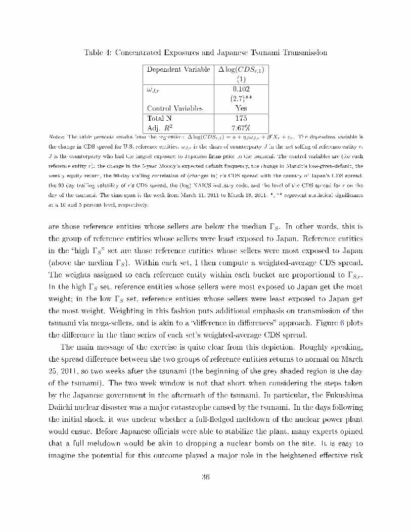
Table 4: Concentrated Exposures and Japanese Tsunami Transmission

Dependent Variable ∆ log(CDSr,1)

(1)

ωJ,r 0.102

(2.7)**

Control Variables YesTotal N 175Adj. R2 7.67%

Notes: The table presents results from the regression: ∆ log(CDSr,1) = a + ηJωJ,r + β′Xr + εr. The dependent variable is

the change in CDS spread for U.S. reference entities. ωJ,r is the share of counterparty J in the net selling of reference entity r.

J is the counterparty who had the largest exposure to Japanese �rms prior to the tsunami. The control variables are (for each

reference entity r): the change in the 5-year Moody's expected default frequency, the change in Markit's loss-given-default, the

weekly equity return, the 90-day trailing correlation of (changes in) r's CDS spread with the country of Japan's CDS spread,

the 90-day trailing volatility of r's CDS spread, the (log) NAICS industry code, and the level of the CDS spread for r on the

day of the tsunami. The time span is the week from March 11, 2011 to March 18, 2011. *, ** represent statistical signi�cance

at a 10 and 5 percent level, respectively.

are those reference entities whose sellers are below the median ΓS. In other words, this is

the group of reference entities whose sellers were least exposed to Japan. Reference entities

in the �high ΓS� set are those reference entities whose sellers were most exposed to Japan

(above the median ΓS). Within each set, I then compute a weighted-average CDS spread.

The weights assigned to each reference entity within each bucket are proportional to ΓS,r.

In the high ΓS set, reference entities whose sellers were most exposed to Japan get the most

weight; in the low ΓS set, reference entities whose sellers were least exposed to Japan get

the most weight. Weighting in this fashion puts additional emphasis on transmission of the

tsunami via mega-sellers, and is akin to a �di�erence in di�erences� approach. Figure 6 plots

the di�erence in the time series of each set's weighted-average CDS spread.

The main message of the exercise is quite clear from this depiction. Roughly speaking,

the spread di�erence between the two groups of reference entities returns to normal on March

25, 2011, so two weeks after the tsunami (the beginning of the grey shaded region is the day

of the tsunami). The two week window is not that short when considering the steps taken

by the Japanese government in the aftermath of the tsunami. In particular, the Fukushima

Daiichi nuclear disaster was a major catastrophe caused by the tsunami. In the days following

the initial shock, it was unclear whether a full-�edged meltdown of the nuclear power plant

would ensue. Before Japanese o�cials were able to stabilize the plant, many experts opined

that a full meltdown would be akin to dropping a nuclear bomb on the site. It is easy to

imagine the potential for this outcome played a major role in the heightened e�ective risk

36

Figure 6: How Long Did the Shock of the Tsunami Last?

08 01Apr2011

09 10 11 14 15 16 17 18 21 22 23 24 25 28 29 30 3156

57

58

59

60

61

62

63

64

Sp

read

(bp

s)

Avg CDS High ΓS - Low ΓS

Notes: This �gure shows the di�erence between the weighted-average CDS spread of high ΓS,r reference entities and low ΓS,r

reference entities. High (low) ΓS,r reference entities are those whose sellers were most (least) exposed to Japanese �rms. The

weights assigned to each reference entity within each bucket are proportional to ΓS,r. The shaded region begins on the day of

the tsunami, March 11, 2011. The shaded region ends on March 25, 2011.

aversion for U.S. sellers who were exposed to Japanese �rms. By March 25, the Fukushima

plant had been relatively stabilized, and the likelihood of a full meltdown dropped sharply.

This resulted in a rebound of risk bearing capacity, which was accompanied by the spread

di�erence between high ΓS and low ΓS reference entities returning to normal.

The length of the e�ect should also be interpreted in conjunction with the size of Japanese

�rm exposure to the overall exposures of each mega-seller or mega-buyer. As mentioned,

I present rough magnitudes of this relative size in Appendix C.1, but loosely speaking, for

mega-sellers of U.S. CDS, Japanese exposures were roughly 4 to 6 percent of their overall

portfolio. While this certainly not trivial, one would also not expect the shock of the tsunami

to have an enormous e�ect on their overall risk bearing capacity. In reality, the shock of the

tsunami is just one example of a multitude of shocks that are constantly changing the risk

bearing capacity of mega-sellers in the market.

37

6 Identi�cation Using Transaction Prices

In this section, I use empirical methods common to the banking literature to provide an

alternative way of identifying the causal e�ect of mega-seller losses on CDS spreads. My

empirical approach is closely related to the within-�rm estimators used by, for example,

Khwaja and Mian (2008), Chodorow-Reich (2014), or Schnabl (2012). Broadly speaking,

these papers try to measure how negative shocks to banks are transmitted to the real economy

via lending relationships. In a similar vein, I am trying to measure how depressed risk bearing

capacity of mega-sellers is transmitted to CDS prices.

My analysis here is inherently di�erent from the previous portions of the paper and it is

critical to keep this in mind when interpreting my results. One di�erence is that my current

approach uses data on transactions, whereas my previous exercises used data on CDS spreads

reported by Markit. The latter are representative of quotes, not actual transaction prices.

A second distinction is that my previous analysis focused on the capital and concentration

of ultimate natural sellers of protection. To compute ultimate natural sellers of protection

in the market, I accounted for exposures through single name and index positions. When

looking at transactions, I will not be concerned with whether the seller in a transaction is

also a natural seller of protection. My objective in examining transactions is only to check

whether there is micro-level evidence that capital losses for a seller are indeed followed by

higher transaction prices.

6.1 Empirical Strategy

To frame the identi�cation problem, suppose CDSit is the spread in transaction i on date t.

The determinants of this spread can be characterized by an arbitrary function, g(·):

log (CDSit) = g(Hrt , H

bt , RB

sit;Xit

)where Hr

t are determinants of CDS spreads that are �rm-speci�c or common to the macroe-

conomy; Hbt are buyer characteristics that determine the CDS spread; RB

sit is the risk bearing

capacity of the seller in transaction i, which I will de�ne shortly; Xit is a vector of transaction

characteristics. These characteristics are the maturity m, log-notional n, and �xed coupon

of the transaction f . I work in logs to avoid econometric issues that arise from the fact that

CDS spreads are bounded below by zero.

I am interested in estimating η = ∂ log(CDSit)/∂RBsit, with the expectation that η < 0.

38

To estimate this e�ect consistently, I must � at a minimum � control for all unobserved

heterogeneity in the cross-section of buyers, reference entity, and dates. I do so by introducing

a buyer-reference entity-time �xed e�ect. Formally, this means I estimate the following

empirical model:

log (CDSit) = αrtb + ηRBsit + εit (10)

where αrtb is the aforementioned �xed e�ect for a reference entity-buyer-time triplet. To

further illustrate the logic of the regression, suppose Hedge Fund A purchases CDS on GE

on date t from multiple sellers. Because I am looking within a buyer, date, and reference

entity, any variation in the transacted CDS spread must be driven by seller characteristics

or other observable characteristics in the transaction. The argument then goes that sellers

with lower risk bearing capacity charge a higher premium.

The risk bearing capacity measure, RBsit, is a function of the CDS portfolio value of seller

s in transaction i, though I choose not to use the actual portfolio value, Vst, for two reasons.

On the econometric side, it is a near unit root and, unlike in my previous analysis, I cannot

take �rst di�erences across transactions. Second, because I am �xing a buyer, reference

entity, and date, there will be substantial scale e�ects if a buyer faces two very di�erently

sized sellers.

To address these issues, I construct RBsit by giving extra weight to dollar losses on recently

open positions and normalizing dollar values by the total gross size of each counterparty's

CDS portfolio. The full details are located in Appendix D.3. The resulting RBsit measure is

still to be interpreted as a measure of portfolio performance, but it has better econometric

properties than the level of dollar values and makes a comparison of di�erent sized sellers

more reasonable because it is normalized by gross values.

6.2 Data Description

As mentioned, the data I use comes from actual transactions. The transaction information

provided by the DTCC contains information on the upfront money paid by the buyer to the

seller at the inception date, or vice versa. A swap is, in theory, initially a zero NPV trade;

the CDS spread we typically think of is the premium the buyer pays to the seller in order

to make the value of default protection exactly equal to the value of the premiums.

In practice, things are slightly more complicated. It is standard in CDS markets for the

buyer to instead pay the seller a �xed coupon, f . If the fair value CDS spread is, for instance

greater than f , then it means the buyer of protection is paying less than she should for the

39

Table 5: CDS Transaction Prices After Seller and Buyer Losses

Dependent Variable log(CDSit)(1) (2)

RBsit -0.019 -0.011

(-4.3)** (-3.1)**log(Notionalit) 0.034

(4.1)**Maturityit -0.07

(-4.4)**FixedRateit 0.51

(18.0)**FE (b, r, t) (b, r, t)Total N 31,872 31,872Within R2 .1% 20.8%

Notes: This table contains the result of the regression: log (CDSit) = αrtb + ηRBsit + εit. CDSit is the implied CDS-spread

(or rather hazard rate) in transaction i. RBsit is the risk bearing capacity of the seller s in the transaction, de�ned as s's total

annualized CDS portfolio return. RBbit is analogously de�ned. Transactions span February 2010 to June 2014, and are �ltered

according to the steps outlined in Section 3 of the Data Appendix. All standard errors clustered by seller. *, ** represent

statistical signi�cance at a 10 and 5 percent level, respectively.

default insurance she receives. In this case, the buyer pays the seller an amount upfront

that makes the total NPV of the swap zero. In my data, I observe this upfront amount.

In Section 3 of the Data Appendix, I document a simple way to transform an observed

upfront amount to an implied hazard rate for the swap. This is important, as it allows me

to compare transactions within the same (b, r, t) group that have di�erent maturities and

�xed coupon amounts. In the same appendix, I also provide additional information for how

I �lter transactions and build the �nal panel data to test the speci�cation in Equation (10).

I consider transactions on all types of CDS (single name, index, and tranche) because

my within buyer-reference entity-time estimator already distinguishes product types. This

is another reason the results I will present are not comparable to those in Section 4.

6.3 Results

Table 5 presents the results of the regression of Equation (10).

Column (1) of the table indicates a one standard deviation increase in seller losses results

in an implied CDS spread increase of roughly 2 percent. Column (2) adds other observable

features of each transaction such as the notional, maturity, and �xed coupon. Interestingly,

the implied CDS spread is increasing in the notional of the transaction, which indicates that

40

sellers who take on a bigger exposure earn an added premium for doing so. One possible

explanation is that traders often face risk limits, so they require an added premium to �ll

larger orders. This idea also rationalizes why we may observe a buyer facing multiple sellers

on the same day and reference entity in the �rst place. If a buyer wishes to �ll a large order

size, it may have to contact multiple sellers to fully �ll the quantity.43 The more important

takeaway is that the coe�cient on RBsit is still large, negative, and signi�cant after the

inclusion of these observable transaction characteristics. A one standard deviation loss to

sellers still results in an 1.1 percent increase in the implied CDS spread of a transaction,

indicating that capital losses a�ect pricing even at a micro-level.

An additional wrinkle is that when the risk bearing capacity of a seller is low, he may

choose to not participate in the market. I con�rm this using a simple logit regression in the

Online Appendix. In this case, we won't observe any transactions with this counterparty,

but that does not mean Markit-reported CDS spreads cannot be high. This is because the

Markit-reported CDS spread is a function of transactions and quotes. Indeed, one way that

sellers can withdraw from the market is to post very high quotes to discourage buyers. As

a result, the e�ect I wish to draw should be even harder to detect using transactional data,

which makes my results more likely to be conservative. In this sense, the results from the

2011 Japanese tsunami in Section 5 are more useful for analyzing how a shock to the risk

bearing capacity of mega-players a�ects quotes (i.e. those reported by Markit).

Is It Just Counterparty Risk?

A natural set of objections to the results in Table 5 relate to the issue of counterparty

risk. Counterparty risk is the risk that the seller (or buyer) will default on their payments in

the CDS. Indeed, Arora, Gandhi, and Longsta� (2012) �nd some evidence of counterparty

risk a�ecting prices, but the size of their e�ect is quite small. Nonetheless, consider two cases

where this might be driving CDS spreads. The �rst is RBsit is itself a proxy for counterparty

risk � sellers who have lost a lot of money are bad counterparties. In this case, though, we

would expect the coe�cient η in the regression to be positive, not negative. Sellers with high

RBsit are good counterparties, and thus can earn a higher premium from buyers. Clearly,

the results of Table 5 contradict this story.

The second case is that I have an omitted variable bias. In this case, the �true� regression

43In addition, buyer-seller relationships are �sticky� as in banking. In the Online Appendix, I show thatthe average non-dealer faces only three di�erent counterparties.

41

speci�cation should be:

cdsit(b, r, t, s,m, n, f) = αrtb + ηRBsit + γCP s

it + εit

where CP sit measures counterparty risk of the seller in transaction i, and is high when s is

a bad counterparty. To think about the direction of the omitted variable bias, �rst notice

that we would expect γ < 0 because bad counterparties must accept lower CDS premiums.

Second, it should be the case that corr(RBsit, CP

sit) < 0 because sellers with high risk bearing

capacity are not likely to be bad counterparties. Denote the estimated coe�cient on RBsit

when omitting CP sit by η̂, and the true parameter value by η. Classical OLS theory says if

γ < 0 and corr(RBsit, CP

sit) < 0, then η < η̂. In other words, the true coe�cient on RBs

it is

even more negative, which suggests sellers with low risk bearing capacity charge even higher

premiums than the estimates I have reported.

7 Conclusion

7.1 Why Might Capital Be Slow Moving?

A basic message of my paper is that limited risk bearing capital for sellers of CDS protection

strongly a�ects prices � losses at the CDS desks of sellers are followed by subsequent in-

creases in default risk premiums. In this subsection, I discuss why capital losses may impact

risk bearing capacity, or in other words why capital in CDS markets appears �slow-moving�

in the sense of Mitchell, Pedersen, and Pulvino (2007) or Du�e and Strulovici (2012). A

theoretical treatment is given by Acharya, Shin, and Yorulmazer (2013), who show that slow

moving capital arises naturally when agents trade o� holding capital for future arbitrage

pro�ts against their current investment opportunities.

One channel for losses to impact risk aversion is psychological. When traders have lost

signi�cant amounts of money, they may become persistently less aggressive in their future

trading strategies.44 Moreover, there are institutional details that suggest risk bearing ca-

pacity and capital losses are tightly linked.

Risk Limits

Risk management teams of �nancial intermediaries and hedge funds impose risk limits

44A quote from one practitioner: If a market downturn is approaching, �senior management may remindtheir troops to be lean, not be a hero (by giving tight bid-asks), and try to stay neutral.�

42

on the positions taken by traders. There are various inputs that go into deciding the size

of these risk limits such as sensitivity to yield curve changes or credit spread changes (e.g.

DV01).45 These risk limits vary with time. At the onset of a trade, each desk is often given

a notional size of the position they can take. If the position performs well, this limit might

be expanded. On the other hand, if the position does poorly, the limit is tightened. A

contraction of risk limits signi�es a decline in risk bearing capacity. Still, conversations with

regulators and practitioners suggest risk limits adjust slowly (e.g. monthly or quarterly) and

only with large losses, so their impact on risk bearing capacity is likely to be strongest when

combined with other institutional frictions.

Value-at-Risk (VaR)

A related way in which portfolio performance relates to risk bearing capacity is through

value at risk constraints, as in Adrian and Shin (2013). Theoretical treatments of VaR con-

straints use the wealth of the trader as a state variable. Naturally, this wealth depends on

the performance of their portfolio, so as this declines, the constraint becomes tighter. From

a regulatory perspective, dealers are required to hold capital against the VaR of their trad-

ing portfolios, which is itself computed based on forecasting models and historical portfolio

performance. It does not seem far fetched to assume that VaR estimates are revised upward

after a poor trading week or month. Furthermore, an important input to VaR-based risk

management is volatility. If portfolio losses coincide with increases in expected portfolio

volatility, then VaR constraints will also concurrently tighten.46

Funding Constaints

Perhaps the most likely way for capital losses to a�ect risk bearing capacity is through

funding. As described in Du�e, Scheicher, and Vuillemey (2014), swap desks arrange in

advance with their treasury desk for a pool of cash to be used for margin purposes. This

precautionary bu�er gets used up as the portfolio loses money because the desk must make

variation margin payments. Furthermore, if VaR estimates also increase after large portfolio

losses, then regulated entities will have to raise additional capital for regulatory purposes.

In turn, if raising additional capital on short notice is costly, then theory suggests that

desk losses will translate to reduced risk taking capacity. For example, Froot and O'Connell

45Recently, Atkeson, Eisfeldt, and Weill (2014a) use risk limits as a friction to complete risk sharing in atheoretical study of OTC markets. See references therein for even more background.

46This claim is supported by a great deal of empirical evidence that documents a negative correlationbetween volatility and returns in equity markets.

43

(2008) use the notion of costly external �nancing to demonstrate how the internal funds of

intermediaries are important for equilibrium asset prices.47 Froot and Stein (1998) also build

a model of �nancial intermediaries that links portfolio decisions with costly external �nance.

In both settings, costly external �nance and depleted capital make intermediaries more risk

averse with respect to their internal wealth levels.48

Supporting Evidence

I now present some supporting evidence of a link between capital losses and risk bearing

capacity, though a complete investigation is outside the scope of this paper. For illustration,

suppose that the funding friction channel is what connects losses and risk bearing capacity.

Standard economic logic says that obtaining new funding on short notice must be costly,

otherwise the desk would simply replenish the capital pool with no other consequences. So

for losses to a�ect risk bearing capacity, the CDS desk must be losing money precisely when

obtaining new funding is di�cult.

To �esh this idea out empirically, I compute the correlation between changes in the

mark-to-market value of a counterparty c's CDS portfolio and the growth rate of c's market

leverage.49 I restrict myself to the subset of dealers in my sample because I can only compute

leverage measures for these counterparties.

Presumably, dealers with high measured leverage face tighter borrowing constraints. If

the funding friction hypothesis is correct, then negative changes in the CDS portfolio depress

risk bearing capacity because they are also accompanied by increases in external funding

constraints for the dealer (i.e. leverage).50 Furthermore, this link should be the tightest

when the desk has already experienced signi�cant losses. As such, I also compute conditional

correlations for each dealer, where I condition on whether mark-to-market values are in their

6-month 10 percent tail.51 Figure 7 illustrates the results, with each pair of bars in the plot

47Interestingly, they also �nd that the market share of intermediaries will be increasing in the cost ofexternal funding, due to increasing returns to scale. This theoretical result seems appropriate for CDSmarkets as well.

48Furthermore, the issue of how funding costs a�ect derivatives valuations has been controversial post-crisis, with most of the debate centered around �funding valuation adjustments (FVA)� for valuing creditderivatives. Hull and White (2014) provide a detailed overview of the potential issues.

49I measure leverage as the ratio of book value of debt to market value of equity.50One might worry that leverage is endogenous and does not accurately re�ect a tightening of borrowing

conditions for a dealer. I have rerun my analysis using other measures of �nancial distress like inverse-equityvolatility (Atkeson, Eisfeldt, and Weill (2014b)) and SRISK (Brownlees and Engle (2014)). The primaryconclusions are robust to these alternatives.

51I compute rolling 6-month changes in the CDS portfolio value, then use the 10 percent quantile as theconditioning event.

44

Figure 7: Correlation Between CDS Portfolio Changes and Market Leverage

Largest Avg. Net Buyer ) Largest Avg. Net Seller�0.8

�0.6

�0.4

�0.2

0.0

0.2

0.4

0.6

⇢(�

Vc

,�

Lev

erage c

)

Unconditional

Conditional

Mega-Sellers

Notes: The �gure computes, for each counterparty c who is a dealer, the correlation between log-changes in market leverage,

∆Leveragec, and the change in the mark-to-market dollar value of the portfolio, ∆Vc. In addition, I compute the conditional

correlation between these two series. The conditioning event is that the trailing 6-month change in Vc,t is in its 10 percent tail.

On the x-axis, each pair of bars corresponds to a single dealer. Dealers are ranked based on their average net exposure, which

for simplicity is computed by summing across all reference entities and counterparties.

corresponding to a single dealer.

The leftmost counterparties in Figure 7 are some of the largest net buyers on average for

the entire market. For most of these dealers, changes in CDS portfolio value are positively

correlated with changes in leverage; when the CDS desk is losing money, the �rm is also in

deleveraging. Thus, we would not expect a decrease in risk bearing capacity to result from

CDS desk losses, given that the dealer is less constrained overall. This intuition is consistent

with my �nding that losses for mega-buyers do not move CDS spreads.

The important portion of Figure 7 is the three rightmost dealers. These dealers are

consistently three of the largest net overall sellers of protection in the market, with their net

position dwar�ng the other dealers who are also sellers. Unconditionally, changes in portfolio

value for these three mega-sellers are about 50 percent negatively correlated with changes in

leverage. In other words, when the desk loses additional money, the dealer's overall leverage

is concurrently increasing. This broadly supports the notion that replenishing the desk's

variation margin pool is costly because losses occur when new funding is relatively di�cult

45

to obtain, or, new capital is slow moving.

The correlations jump substantially when I condition on poor portfolio performance.

When the CDS desks at these three dealers are doing particularly badly, changes in dollar

portfolio value are nearly 80 percent negatively correlated with changes in leverage. This is

exactly what we should see in the data if the funding frictions channel is correct. Of course,

this evidence is observationally equivalent to both a risk limit and VaR story. It is entirely

possible (and highly probable) that as a dealer's leverage is rising, it simultaneously contracts

its risk limits and updates its VaR, which may itself require obtaining additional funds. In

the present context, the exact avenue through which CDS losses depress risk bearing capacity

is a matter of interpretation. In reality, all channels are probably at play.

The size of the CDS portfolios for these mega-sellers is also quite large. For con�dentiality

reasons, I cannot report detailed descriptive statistics of portfolio size. Still, to give a sense

of size, for each dealer I compute the ratio of the absolute value of their CDS portfolio value

to their equity. Across the three dealers and through time, the average CDS-to-equity ratio

is 5 percent, but at some points in the sample it reaches nearly 12 percent. These magnitudes

are sizable given the wide range of activities and asset holdings of these institutions. It is

not hard to argue that �uctuations in the value of the CDS desk for these mega-sellers also

have a substantial impact on their overall wealth.

7.2 Final Remarks

The major contribution of my paper is twofold: �rst, I show that capital �uctuations for

sellers of CDS protection explain a signi�cant amount of variation in default risk premiums.

Intuitively, when seller capital declines, risk premiums rise. This �nding is consistent with

many theoretical models of limited investment capital, though is particularly striking due

to the fact that a handful of CDS sellers account for most of the market. Second, I show

why the distribution of capital, as opposed to only the total amount of capital, matters for

pricing. When sellers become more concentrated, the market becomes more fragile through

an increase in the volatility of risk premiums.

These two �ndings have important policy implications. For one, the fact that the level

of risk bearing capital in a market impacts risk premiums provides a potential rationale

for outside capital injections (e.g. bailouts) when sellers are under-capitalized. Still, this

argument is obviously subject to the usual set of moral hazard objections (as in the case

of too-big-to-fail subsidies). Even in the presence of moral hazard issues, a deeper point is

46

that the distribution of capital injections can also have a substantial impact on pricing. This

follows directly from the fact that concentration leads to higher volatility. In this sense, it

is unlikely that every bailout is equal � where capital injections �ow is also important.

The stylized facts I document about CDS markets also raise potential policy red �ags in

terms of �nancial stability and market design. For instance, consider the highly controversial

government bailout of AIG, who at the time was a large seller of CDS protection on the U.S.

housing market. One of the cited reasons for the bailout in the popular press was that a

failure of AIG could have substantial trickle down e�ects from counterparty risk. As alluded

to in the introduction, much of the post-crisis regulation has aimed to reduce counterparty

risk and increase transparency in derivatives markets though central clearing. Although

these mechanisms are a useful step, the results of this paper highlight that the existence of

mega-sellers has persisted in the aftermath of the crisis.

One way to reduce the concentration inherent to CDS is for the central clearing party

(CCP) to charge, in addition to existing margin requirements, a �concentration margin� that

would penalize counterparties for outsized market shares. Of course, this would require the

CCP to clear all traded swaps so that it could accurately compute market share through

single name and index positions. With that said, it is not obvious what the optimal allocation

of CDS should be from a welfare-maximizing perspective. At a minimum, more research is

necessary to properly assess welfare implications, and in particular, whether new regulation

has done enough to ensure a failure of one of these mega-sellers would not have a signi�cant

impact on �nancial stability. The map of true economic exposures (via CDS) created in this

paper is a useful tool for this task.

Another important aspect of my stylized facts is that selling of CDS has partly moved

from dealers to hedge funds and asset managers. A likely explanation for this pattern is that

new regulation has made it less pro�table (or even possible) for dealers to ultimately bear

credit risk via CDS. Still, it is important to consider whether moving this function to the

largely unregulated sphere of hedge funds and asset managers is optimal from a �nancial

stability perspective.

Regarding CDS market design, the facts uncovered in this paper beg the question: why

is there such limited participation in CDS markets? This question is particularly important

given I have shown that changes in the risk bearing capacity of a small set of sellers in the

market can move CDS spreads by a substantial amount. The next step is to understand how

and why the concentrated market structure of CDS arises endogenously.

47

References

Viral Acharya, Stephen Schaefer, and Yili Zhang. Liquidity risk and correlation risk: A clinicalstudy of the general motors and ford downgrade of 2005. Forthcoming: Quarterly Review ofFinance, 2014.

Viral V. Acharya, Hyun Song Shin, and Tanju Yorulmazer. A theory of arbitrage capital. Reviewof Corporate Finance Studies, 2013.

Tobias Adrian and Nina Boyarchenko. Intermediary leverage cycles and �nancial stability. FederalReserve Sta� Report, (567), 2013.

Tobias Adrian and Hyun Song Shin. Procyclical leverage and value-at-risk. Review of FinancialStudies, 2013.

Tobias Adrian, Paolo Colla, and Hyun Song Shin. Which �nancial frictions? Parsing the evidencefrom the �nancial crisis of 2007-09. Sta� Reports 528, Federal Reserve Bank of New York, 2011.

Tobias Adrian, Erkko Etula, and Tyler Muir. Financial intermediaries and the cross-section of assetreturns. The Journal of Finance, page Forthcoming, 2014.

Miguel Anton and Chistopher Polk. Connected stocks. The Journal of Finance, 69(3):1099�1127,2014. ISSN 1540-6261.

Navneet Arora, Priyank Gandhi, and Francis A. Longsta�. Counterparty credit risk and the creditdefault swap market. Journal of Financial Economics, 103(2):280 � 293, 2012. URL http:

//www.sciencedirect.com/science/article/pii/S0304405X11002327.

Andrew Atkeson, Andrea Eisfeldt, and Pierre-Olivier Weill. The market for otc derivatives. WorkingPaper, url: https://sites.google.com/site/andrealeisfeldt/, 2013.

Andrew Atkeson, Andrea Eisfeldt, and Pierre-Olivier Weill. Entry and exit in otc derivativesmarkets. Working Paper, url: https://sites.google.com/site/andrealeisfeldt/, 2014a.

Andrew Atkeson, Andrea Eisfeldt, and Pierre-Olivier Weill. Measuring the �nancial soundness ofu.s. �rms, 1926-2012. Working Paper, url: https://sites.google.com/site/andrealeisfeldt/, 2014b.

Robert L. Axtell. Zipf distribution of u.s. �rm sizes. Science, 293(5536):1818�1820, 2001. doi: 10.1126/science.1062081. URL http://www.sciencemag.org/content/293/5536/1818.abstract.

Jennie Bai and Pierre Collin-Dufresne. The cds-bond basis. SSRN:http://ssrn.com/abstract=2024531, 2013.

Jennie Bai and Liuren Wu. Anchoring credit default swap spreads to �rm fundamentals. SSRN:http://ssrn.com/abstract=2020841, 2012.

Jack Bao and Jun Pan. Bond illiquidity and excess volatility. Review of Financial Studies, 2013.doi: 10.1093/rfs/hht037. URL http://rfs.oxfordjournals.org/content/early/2013/07/04/

rfs.hht037.abstract.

48

Antje Berndt, Rohan Douglas, Darrell Du�e, Mark Ferguson, and David Schranz. Measuringdefault risk premia from default swap rates and edfs. SSRN: http://ssrn.com/abstract=556080,2008.

Christian T. Brownlees and Robert F. Engle. Volatility, correlation and tails for systemic riskmeasurement. Working Paper, SSRN: http://ssrn.com/abstract=1611229, 2014.

Markus K Brunnermeier and Yuliy Sannikov. A macroeconomic model with a �nancial sector. TheAmerican Economic Review, 104(2):379�421, 2014.

John Y. Campbell and Robert J. Shiller. Stock prices, earnings, and expected dividends. The Journalof Finance, 43(3):661�676, 1988. ISSN 1540-6261. doi: 10.1111/j.1540-6261.1988.tb04598.x. URLhttp://dx.doi.org/10.1111/j.1540-6261.1988.tb04598.x.

Peter Carr and Liuren Wu. A simple robust link between american puts and credit protection.Review of Financial Studies, 24(2):473�505, 2011. doi: 10.1093/rfs/hhq129. URL http://rfs.

oxfordjournals.org/content/24/2/473.abstract.

Hui Chen, Rui Cui, Zhiguo He, and Konstantin Milbradt. Quantifying liquidityand default risks of corporate bonds over the business cycle. Working Paper, url:http://www.mit.edu/ huichen/bondliquidity.pdf, 2014a.

Hui Chen, Scott Joslin, and Sophie X. Ni. Demand for Crash Insurance, Intermediary Con-straints, and Risk Premia in Financial Markets. SSRN, 2014b. URL http://ssrn.com/abstract=

2024416.

Kathryn Chen, Michael Fleming, John Jackson, Ada Li, and Asani Sarka. An analysis of cdstransactions: Implications for public reporting. NY Fed Working Paper, (517), 2011.

Long Chen, Pierre Collin-Dufresne, and Robert S. Goldstein. On the relation between the creditspread puzzle and the equity premium puzzle. Review of Financial Studies, 22(9):3367�3409,2009. doi: 10.1093/rfs/hhn078. URL http://rfs.oxfordjournals.org/content/22/9/3367.

abstract.

Gabriel Chodorow-Reich. The employment e�ects of credit market disruptions: Firm-level evidencefrom the 2008-09 �nancial crisis. Quarterly Journal of Economics, 129:1�59, 2014.

In Choi. Unit root tests for panel data. Journal of International Money and Finance, 20(2):249�272,April 2001. URL http://ideas.repec.org/a/eee/jimfin/v20y2001i2p249-272.html.

Pierre Collin-Dufresne, Robert S. Goldstein, and J. Spencer Martin. The determinants of creditspread changes. The Journal of Finance, 56(6):2177�2207, 2001. ISSN 1540-6261. doi: 10.1111/0022-1082.00402. URL http://dx.doi.org/10.1111/0022-1082.00402.

Joshua Coval and Erik Sta�ord. Asset �re sales (and purchases) in equity markets. Journal ofFinancial Economics, 86(2):479�512, 2007.

Joost Driessen. Is default event risk priced in corporate bonds? Review of Financial Studies, 18:165�195, 2005.

49

Gregory R. Du�ee. The relation between treasury yields and corporate bond yield spreads. TheJournal of Finance, 53(6):2225�2241, 1998. ISSN 1540-6261. doi: 10.1111/0022-1082.00089. URLhttp://dx.doi.org/10.1111/0022-1082.00089.

D Du�e and KJ Singleton. Modeling term structures of defaultable bonds. Review of FinancialStudies, 12(4):687�720, 1999. doi: 10.1093/rfs/12.4.687. URL http://rfs.oxfordjournals.

org/content/12/4/687.abstract.

Darrell Du�e. Credit swap valuation. Financial Analysts Journal, pages 73�87, 1999.

Darrell Du�e. Presidential address: Asset price dynamics with slow-moving capital. The Journalof Finance, 65(4):1237�1267, 2010.

Darrell Du�e and Bruno Strulovici. Capital mobility and asset pricing. Econometrica, 80(6):2469�2509, 2012.

Darrell Du�e, Ada Li, and Theo Lubke. Policy perspectives on otc derivatives market infrastructure.Federal Reserve Sta� Report, (424), 2011.

Darrell Du�e, Martin Scheicher, and Guillaume Vuillemey. Central clearing and collateral demand.Forthcoming: Journal of Financial Economics, 2014.

Edwin J. Elton, Martin J. Gruber, Deepak Agrawal, and Christopher Mann. Explaining the ratespread on corporate bonds. The Journal of Finance, 56(1):247�277, 2001. ISSN 1540-6261. doi:10.1111/0022-1082.00324. URL http://dx.doi.org/10.1111/0022-1082.00324.

Jan Ericsson, Kris Jacobs, and Rodolfo Oviedo. The determinants of credit default swap premia.Journal of Financial and Quantitative Analysis, 44(01):109�132, 2009.

Kenneth Froot and Paul O'Connell. On the pricing of intermediated risks: Theory and applicationto catastrophe reinsurance. Special Issue on Dynamics of Insurance Markets: Structure, Conduct,and Performance in the 21st Century Journal of Banking and Finance, 32(1):69�85, 2008.

Kenneth Froot, John Arabadjis, Sonya Cates, and Stephen Lawrence. How institutional investorsframe their losses: Evidence on dynamic loss aversion from currency portfolios. Journal of Port-folio Management, 38(2):60�68, 2011.

Kenneth A. Froot and Paul G. J. O'Connell. The Pricing of U.S. Catastrophe Reinsurance. pages195�232, 1999.

Kenneth A. Froot and Jeremy C. Stein. Risk management, capital budgeting, and capital structurepolicy for �nancial institutions: an integrated approach. Journal of Financial Economics, 47(1):55�82, 1998.

Kenneth A. Froot, David S. Scharfstein, and Jeremy C. Stein. Risk management: Coordinatingcorporate investment and �nancing policies. The Journal of Finance, 48(5):1629�1658, 1993.ISSN 1540-6261. doi: 10.1111/j.1540-6261.1993.tb05123.x. URL http://dx.doi.org/10.1111/

j.1540-6261.1993.tb05123.x.

50

Xavier Gabaix. The granular origins of aggregate �uctuations. Econometrica, 79(3):733�772, 2011.ISSN 1468-0262. doi: 10.3982/ECTA8769. URL http://dx.doi.org/10.3982/ECTA8769.

Xavier Gabaix and Rustam Ibragimov. Rank 1/2: A simple way to improve the ols estimation oftail exponents. Journal of Business and Economic Statistics, 29(1):24�39, 2011.

Xavier Gabaix, Arvind Krishnamurthy, and Olivier Vigneron. Limits of arbitrage: Theory andevidence from the mortgage-backed securities market. The Journal of Finance, 62(2):557�595,2007.

Simon Gilchrist and Egon Zakrajsek. Credit spreads and business cycle �uctuations. AmericanEconomic Review, 102(4):1692�1720, 2012. doi: 10.1257/aer.102.4.1692. URL http://www.

aeaweb.org/articles.php?doi=10.1257/aer.102.4.1692.

C.W.J. Granger and P. Newbold. Spurious regressions in econometrics. Journal of Econometrics, 2(2):111 � 120, 1974.

Richard C. Green, Burton Holli�eld, and Norman Schurho�. Financial intermediation and the costsof trading in an opaque market. Review of Financial Studies, 20(2):275�314, 2007.

Robin Greenwood and David Thesmar. Stock price fragility. Journal of Financial Economics, 102(3):471 � 490, 2011. ISSN 0304-405X. doi: http://dx.doi.org/10.1016/j.j�neco.2011.06.003. URLhttp://www.sciencedirect.com/science/article/pii/S0304405X11001474.

Denis Gromb and Dimitri Vayanos. Equilibrium and welfare in markets with �nancially constrainedarbitrageurs. Journal of Financial Economics, 66:361 � 407, 2002.

Samuel G. Hanson and Adi Sunderam. The growth and limits of arbitrage: Evidence from shortinterest. Review of Financial Studies, 2013.

Zhiguo He and Arvind Krishnamurthy. Intermediary asset pricing. American Economic Review,103(2):732�70, 2013. doi: 10.1257/aer.103.2.732. URL http://www.aeaweb.org/articles.php?

doi=10.1257/aer.103.2.732.

John Hull and Alan White. Valuing derivatives: Funding value adjustments and fair value. Forth-coming: Financial Analysts Journal, 2014.

Robert A. Jarrow and Stuart M. Turnbull. Pricing derivatives on �nancial securities subject to creditrisk. The Journal of Finance, 50(1):53�85, 1995. ISSN 1540-6261. doi: 10.1111/j.1540-6261.1995.tb05167.x. URL http://dx.doi.org/10.1111/j.1540-6261.1995.tb05167.x.

Bryan Kelly, Hanno Lustig, and Stijn Van Nieuwerburgh. Firm volatility in granular networks.Working Paper, SSRN: http://ssrn.com/abstract=2186197, 2014.

Asim Ijaz Khwaja and Atif Mian. Tracing the impact of bank liquidity shocks: Evidence from anemerging market. American Economic Review, 98(4):1413�42, 2008.

Albert S. Kyle and Wei Xiong. Contagion as a wealth e�ect. The Journal of Finance, 56(4):1401�1440, 2001.

51

Matteo Maggiori. Financial intermediation, international risk sharing, and reserve currencies. Un-published manuscript, UC Berkeley, 2011.

Robert C. Merton. On the pricing of corporate debt: The risk structure of interest rates. TheJournal of Finance, 29(2):449�470, 1974.

Robert C. Merton. A simple model of capital market equilibrium with incomplete information. TheJournal of Finance, 42(3):483�510, 1987.

Mark Mitchell, Lasse Heje Pedersen, and Todd Pulvino. Slow moving capital. American EconomicReview, 97(2):215�220, 2007.

Amrut Nashikkar and Lasse Pedersen. Corporate bond specialness. Working Paper, SSRN:http://ssrn.com/abstract=967545, 2007.

Yigal Newman and Michael Rierson. Illiquidity spillovers: theory and evidence from europeantelecom bond issuance. Stanford University Working Paper, 2004.

Martin Oehmke and Adam Zawadowski. The anatomy of the cds market. SSRN:http://ssrn.com/abstract=2023108, 2013.

Martin Oehmke and Adam Zawadowski. Synthetic or real? the equilib-rium e�ects of credit default swaps on bond markets. Working Paper, url:https://www0.gsb.columbia.edu/faculty/moehmke/papers/OehmkeZawadowskiCDSvsBonds.pdf,2014.

Or Schachar. Exposing the exposed: Intermediation capacity in the credit default swap market.NY Fed Working Paper, 2012.

Philipp Schnabl. The international transmission of bank liquidity shocks: Evidence from an emerg-ing market. The Journal of Finance, 67(3):897�932, 2012.

Andrei Shleifer and Robert W Vishny. The limits of arbitrage. The Journal of Finance, 52(1):35�55, 1997.

Dragon Tang and Hong Yan. What moves cds spreads? Working Paper:http://www.sef.hku.hk/ yjtang/TangYan-CDSMove_21Jun2013.pdf, 2013.

52

A Capital Fluctuations and the Pricing of Credit Risk:

Complimentary Evidence

In this section, I provide empirical results that are intended to compliment the main analysis in Section 4.I �rst show that capital losses for all sellers (not just mega-sellers) are followed by increases in the price ofcredit risk, Πt. As a part of this analysis, I con�rm that mega-seller capital losses a�ect the price of creditrisk in the same way that total capital �uctuations of natural sellers do, a natural �nding given the marketshare of mega-sellers. On the other hand, I also show that Πt responds di�erently to a loss at an �average�seller compared to a loss at a mega-seller, thereby providing another piece of evidence that the distributionof capital is important for pricing. The last exercise of this section builds on this idea by showing thatidiosyncratic dollar shocks at the largest sellers move default risk premiums.

A.1 The Price of Credit Risk and Aggregate Risk Bearing Capital

My �rst task is to link time-variation in πt = log(Πt) to variation in the risk-bearing capital of natural sellersof CDS. In Section 4.1, I established this link by using a panel of CDS spreads. The obvious advantage of apanel is that it takes advantage of both cross-sectional and time-series variation.

To support those �ndings, I now take a more �macro� approach to the same question. At each time t, Icompute the total market value of all natural seller positions simply by summing across the market value ofeach natural seller's CDS portfolio, Vct:

Vt =∑c∈As

t

Vct

where, again, I identify natural sellers of CDS as the set of counterparties with a positive aggregate marketshare as de�ned in Section 3.2. To ensure that I do not include traders who switch between net buying andselling of protection, I only include counterparties who are above the 20th percentile in terms of aggregatemarket share. With some abuse of notation, I denote this set of sellers by As

t .I view Vt as a good proxy for the net overall wealth of natural sellers because, again, it is di�cult to

directly hedge a sold CDS position.52 The following regression then tests the extent to which variation inthe price of credit risk are generated by changes in aggregate risk bearing capital:

∆πt = a+ ρ∆πt−1 + Λ′[∆Xt] + φ [∆Vt−1] + et (11)

where Xt is the same vector of macroeconomic controls used in my prior analysis. As a reminder, these arethe log equity-to-price ratio for the S&P 500, VIX, TED, CFNAI, 10 year Treasury yield, 10 year minus2 year treasury yield, and the CBOE Option Skew index. After �rst di�erencing these aforementionedvariables, I also include the excess market return of the CRSP value-weighted index.53

In Section 4.1, I avoided reverse causality concerns by looking at whether losses outside of a referenceentity's industry impact the pricing of that reference entity. Clearly, this strategy is only possible when usinga panel of CDS spreads. Thus, to avoid any reverse causality issues in my current setup, I simply lag thechange in seller capital regression (11). Based on these earlier empirical results and on theoretical modelswith slow-moving capital or limited �nancial intermediary risk bearing capacity, we would expect φ < 0.When natural sellers lose capital, CDS premiums should subsequently rise. Table 6 collects the results ofregression (11).

52As long as Vt is correlated with overall wealth, theoretical models with limited risk bearing capitalsuggest it should be important for determining risk premiums.

53This may seem redundant to including the log-change in the S&P 500 index, but I do so in order toaccount for higher frequency (weekly) equity movements. The earnings-to-price ratio is monthly and takenfrom Robert Shiller's website.

53

Table 6: The Price of Credit Risk and P&L of All Natural Sellers

Dep. Variable ∆πt(1) (2) (3) (4)

∆Vt−1 -0.007 -0.007(-2.8)** (-2.7)**

∆Vt−1 × 1∆Vt−1≥0 -0.005(-1.43)

∆Vt−1 × 1∆Vt−1<0 -0.009(-2.57)**

∆Vt−1 ×∆TEDt−1 -0.003(-1.9)*

Macro Controls Yes Yes Yes YesAdj. R2 21.0 24.0 24.0 23.0

N 190 190 190 190Notes: This table presents results from estimating variants of the regression: ∆πt = a+ ρ∆πt−1 + Λ

′[∆Xt] + φ [∆Vt−1] + et.

∆Vt−1 is the change in the mark-to-market value of the CDS positions for natural sellers of CDS protection from t − 1 to t.

Natural sellers are determined each period as those counterparties whose aggregate market share (de�ned in Section 3.2) is

above the 20th percentile. ∆TEDt is the change TED spread over the same time span. All variables have been transformed

to have a mean of zero and variance of one. **,* indicates coe�cient is statistically di�erent than zero at the 5 percent and 10

percent con�dence level, respectively.

Column (1) of Table 6 shows the results of regression changes in πt on its own lag and only the macroe-conomic variables. The R2 from this speci�cation is 21 percent, or in other words, macroeconomic variablescan explain about a �fth of the variation in the price of credit risk. Column (2) adds the lagged changein seller capital to the regression. The point estimate is statistically signi�cant at conventional levels, andthe negative sign con�rms our intuition that capital losses result in increases in aggregate premiums. Theincremental R2 from this regression is 3 percent, which is large given the limited explanatory power bymacroeconomic variables of changes in πt.

I incorporate the potential for a non-linear relationship between capital and the price of credit risk intoregression (11) in two ways. First, I allow lagged changes in aggregate seller capital to have di�erential e�ectson ∆πt, depending on whether capital increases or decreases. I accomplish this by interacting ∆Vt−1 withan indicator variable for whether it is positive or negative. As column (3) suggests, there is an asymmetricale�ect of capital losses on the price of credit risk. In absolute value, the price of credit risk rises almost twiceas much following a loss, relative to how much it drops following a capital gain.54 Again, this is exactly whatwe would expect in lieu of the theoretical results from models like He and Krishnamurthy (2013).

The second way I incorporate non-linearity is by interacting lagged changes in aggregate seller capitalwith changes in the TED spread. Because the TED spread is often used as a proxy for the funding conditionsof the banking sector, this interaction term captures situations where natural sellers lose capital and fundingconditions tighten. Following with intuition, column (4) shows that capital losses have their strongest e�ecton the price of credit risk when funding conditions are simultaneously tightening. For instance, if a onestandard deviation increase in the TED spread is accompanied by a one standard deviation deduction in

54These relative magnitudes are larger than those found in my panel analysis in Section 4.1. This isplausibly attributed to the fact that Section 4.1 examines contemporaneous changes in CDS spreads andlosses, whereas the present analysis uses lags.

54

seller capital, the price of risk rises by about one percent in the following week.55

A Simple Variance Decomposition

The goal of the previous set of regressions was to establish that capital losses to natural sellers of protectionare followed by increases in default risk premiums. The results from that exercise also suggest that shocks

to the price of credit risk are likely driven by either shocks to macroeconomic fundamentals or shocks to therisk bearing capital of natural sellers. To get a better sense of what is behind variability in shocks to Πt, Iuse a forecast error variance decomposition from the following �rst order unrestricted vector autoregression(VAR):

yt = c + Φ′yt−1 + et

yt :=[Xt Vt Πt

]′where the lag structure in the VAR was chosen by standard information criterion. I recursively order thevariables in the VAR under the assumption that a shock to natural seller capital levels a�ects the price ofcredit risk with a lag, while macroeconomic variables can react contemporaneously to such a shock. I havefurther veri�ed that the estimated VAR coe�cient matrix Φ is stable in the sense that all of its eigenvalueshave a modulus less than one.

Figure 8 displays the amount of variation in Πt explained by an orthogonalized one standard deviationshock to natural seller capital. An orthogonal innovation to natural seller capital accounts for about 20percent of the variation of shocks to the price of credit risk. In other words, about one-�fth of unexpectedchanges in the price of credit risk can be attributed to shocks to the capital of natural CDS sellers. Theseresults compliment my earlier �nding in Section 4.1 that �uctuations in mega-seller capital explain aboutone-ninth of the �uctuations in contemporaneous CDS spread changes, with the di�erence likely due to thefact that CDS spreads are (almost mechanically) noisier than Πt.

Interpretation

One might argue that because swaps are in zero-net supply, losses to natural sellers of protection are equiva-lent to gains for natural buyers of protection. In turn, it is really the gains of buyers that causes an increasein aggregate CDS premiums. To see why an increase in buyer wealth may a�ect risk premiums, consider thefollowing sketch of a model: existing buyers and sellers of CDS di�er in their opinions about the likelihoodof default, with buyers more pessimistic about default likelihoods than sellers. When a news shock occursthat increases default probabilities, equilibrium CDS spreads rise and wealth gets transferred from sellers tobuyers due to mark-to-market changes. Because the wealth-weighted average expected default likelihood isnow higher, the premium for bearing default risk subsequently rises even more.56

In this example, the capital of natural sellers is not the true determinant of variations in aggregatedefault risk premiums, but seller losses would nonetheless correspond to increases in risk premiums. In analternative view of the world, it could be the case that the demand for protection is perfectly inelastic inprice, maybe because buyers of CDS purchase protection in �xed quantity to hedge a constant portion oftheir underlying bond portfolio. In this case, a decrease in seller wealth limits their willingness or ability tobear additional risk, thereby increasing the price of credit risk.

There are few reasons why I believe my results support the notion that seller losses, and not buyer gains,economically determine CDS premiums. First, and most importantly, the identi�cation exercises I explorein other portions of the paper support this claim. Second, if buyer wealth is really moving risk premiums,

55The standard deviation of log-changes in the price of credit risk is about 2 percent. So in other words, aone standard deviation event in capital losses and TED spread changes this week produces an e�ect on theprice of credit risk on the order of 50 percent of a standard deviation next week.

56I thank Xavier Gabaix for a very useful discussion of this possibility.

55

Figure 8: Forecast Error Variance Decomposition of Seller Capital Shock

-20

-10

0

10

20

30

40

50

60

2 4 6 8 10 12 14 16 18 20 22 24 26 28 30

Horizon

Perc

ent

of

Price o

f C

redit R

isk V

ariance d

ue t

o S

eller

Shock

Notes: This �gure plots portion of the forecast error variance of the price of credit risk Πt explained by shocks to natural

seller capital.The VAR was orthogonalized using the Cholesky decomposition with the following ordering: CFNAI index, 10Y

treasury yield, 10Y-2Y treasury yield, VIX, TED, CBOE Option Skew index, earnings-to-price ratio, CRSP Value-Weighted

Excess Market Return, natural seller capital Vt, and the price of credit risk Πt.The system was estimated using weekly data from

February 2010 to June 2014. The variance decomposition is robust to alternative orderings of the macroeconomic variables.

then we would not observe an asymmetric response of risk premiums to natural seller losses. Moreover,there is no reason to believe that buyer gains should have a stronger a�ect on the price of risk when fundingconditions for banks are worsening, as is the case in column (4) of Table 6. Finally, because I am unable toobserve the joint bond-CDS portfolio of buyers, it is not entirely clear that a gain in CDS actually increasesbuyer wealth. As a result, I adopt the interpretation that changes in the capital of natural CDS sellers drivedynamics in the price of credit risk.

A.2 Concentration and Aggregate Risk Bearing Capital

To con�rm that aggregate risk bearing capacity is largely determined by mega-sellers, in each week t, I mirrorregression (11) by using changes in the capital of the mega-buyers and mega-sellers to explain subsequentchanges in the price of credit risk:

∆πt = a+ ρ∆πt + Λ′[∆Xt] + φS

[∆VMS

t−1]

+ ϕB

[∆VMB

t−1]

+ et (12)

where ∆VMSt is the change in the mark-to-market value of the entire CDS portfolio for mega-sellers from

time t − 1 to t.57 ∆VMBt is the same measure for mega-buyers. I am able to include the capital changes

for the top sellers and buyers in this regression because they are not collinear. This would not be the caseif these counterparties were the only sellers and buyers in the market. Table 7 presents the results of this

57Earlier, I used a similar version of this variable that was reference entity speci�c because it only includedpositions on reference entities outside of a speci�c industry.

56

Table 7: The Price of Credit Risk and P&L of the Largest Sellers

Dep. Variable ∆πt(1) (2) (3) (4)

∆VMBt−1 0.001 0.001

(0.5) (0.52)∆VMS

t−1 -0.008 -0.008(-3.0)** (-3.1)**

∆VABt−1 0.002 0.002(1.0) (1.1)

∆VASt−1 -0.00 -0.002(-0.19) (-0.96)

Macro Controls Yes Yes Yes YesAdj. R2 21.0 24.1 20.7 24.1

N 190 190 190 190Notes: This table presents results from estimating variants of the regression: ∆πt = a + ρ∆πt + Λ

′[∆Xt] + φS

[∆VMS

t−1

]+

ϕB[∆VMB

t−1

]+ et. ∆VMS

t is the change in the mark-to-market value of the entire CDS portfolio for mega-sellers from time

t− 1 to t, and ∆VMBt is the same measure for mega-buyers. In columns (3) and (4), I add the change in CDS portfolio value

for the �average� buyer and seller in the market, denoted by ∆VABt−1 and ∆VASt−1, respectively. The average seller (buyer) is

determined each period as the group of sellers (buyers) whose market share is in the 45-55th percentile. All V variables have

been transformed to have a mean of zero and variance of one. **,* indicates coe�cient is statistically di�erent than zero at the

5 percent and 10 percent con�dence level, respectively.

regression.There are at least two interesting patterns that emerge from Table 7. First, the point estimate on changes

in the market value of mega-buyers' CDS in column (2) is not distinguishable from zero, indicating that thisset of buyers does not drive risk price dynamics. On the other hand, a one standard deviation deduction inthe capital of mega-sellers result in a 0.8 percent increase in the future price of credit risk. Moreover, themagnitude of this e�ect is about the same as a one standard deviation decrease in the aggregate capital ofall natural sellers (compare to column (2), Table 6). This result is not surprising, given that �ve sellers ofCDS account for almost �fty percent of the entire market. However, this is also my point about fragility:the capital level of just �ve protection sellers plays an outsized role in CDS pricing.

The second observation from Table 7 is that a dollar loss at a mega-seller has a di�erent e�ect than adollar loss at an �average� seller. To make this clear, in each period I de�ne the median sellers (buyers) ascounterparties whose market share of aggregate selling (buying) is in the 45-55 percentile.58 I use mediansinstead of averages to avoid the undue in�uence of extremely large and small market shares. I denote thechange in CDS portfolio value for the group of �average� sellers (buyers) by ∆VAS

t (∆VABt ). Column (3)

then includes lags of these variables in regression (12). As the point estimates suggest, there is no discernibleimpact on pricing from �uctuations in average seller or average buyer capital. If the distribution of capitalwas irrelevant and only the aggregate amount of risk bearing capital mattered for pricing, then we would notobserve these results. Column (4) reinforces this idea by including in the regression changes in capital forthe mega-players and the average players. A comparison of the estimated coe�cient on mega-seller versusaverage seller capital changes indicates that the e�ect of a dollar loss on pricing is highly dependent on where

58I use a range, as opposed to a single counterparty, to avoid potential issues stemming from the actualmedian seller changing identities from week to week.

57

this loss occurs.

A.3 Idiosyncratic Losses Cause Spread Movements

A recurring theme of this paper is that the distribution of capital losses (as opposed to just the total amountof capital) for natural sellers is important because it can generate price fragility. In an environment with veryconcentrated sellers, idiosyncratic capital shocks to one seller translate to aggregate capital shocks. Thus,poor performance of an isolated mega-seller can still have large pricing impacts in the aggregate. Indeed, the2012 JP Morgan London Whale is certainly one example of how the entire CDS market can move based onthe actions of a single �rogue� trader. In this subsection, I formalize the logic of the �London Whale� using aslightly more complex econometric methodology that �rst identi�es idiosyncratic shocks to large sellers andthen traces out how these idiosyncratic shocks impact prices.

To start, I regress each counterparty's portfolio changes on a set of systematic factors, denoted by Ft,and save the regression residuals:

∆Vct = ac + β′

cFt + ξct (13)

The key part of this step is choosing the appropriate set of factors, Ft. One approach would be to useeconomic factors such as the excess equity market return or changes in changes in the treasury yield curve.Instead of taking a stance on the important factors that drive portfolio changes, I use principal componentsto choose the factors. Speci�cally, I extract the �rst �ve principal components from a panel of log-CDSspread changes. I use �ve factors because that is the minimum number needed to capture 80 percent ofspread variation, but my results are not sensitive to this choice.59

I treat the residuals, ξct, from this regression as idiosyncratic capital shocks to c's CDS portfolio. I doso because ξct is the portion of c's capital change (from CDS) that cannot be explained by exposure to thesystematic factors, Ft. Next, for each reference entity r I build �buyer and seller granular residuals�, de�nedas:

Ψsrt :=

∑c∈St−1(r)

ωsr,c,t−1ξct

Ψbrt :=

∑c∈Bt−1(r)

ωbr,c,t−1ξct (14)

where St−1(r) and Bt−1(r) are the set of r's sellers and buyers, respectively, at time t− 1. Similarly, ωsr,c,t−1

is counterparty c's share of selling in r at time t−1. ωbr,c,t−1 is de�ned analogously for buyers.

60 In words, Ψsrt

is a share-weighted average of the idiosyncratic dollar shocks for r's net sellers. When r's important sellersare hit with large idiosyncratic dollar shocks, then Ψs

rt will also be large. Ψbrt carries a similar intuition, but

for the important buyers of reference entity r. I call the Ψ variables seller and buyer granular residuals inaccordance with Gabaix (2011).61

59If anything, I am being too stringent in my choice of factors, given that shocks to large sellers couldthemselves be an important factor moving spreads.

60Formally, ωbr,c,t−1 = −NS(c, r, t− 1)/NO(r, t− 1) conditional on NS(c, r, t− 1) < 0. The negative sign

makes buyers have positive weights, since NS < 0 indicates net buying.61The reader may notice that the granular buyer and seller granular residuals in this section are constructed

using the biggest sellers of a particular reference entity r. This construction is in slight contrast to myanalysis of how losses transmit across mega-players' portfolios, where I focus on the top �ve sellers andbuyers in the aggregate. The reason I opt for the two di�erent approaches is for identi�cation. In theprevious section, I am able to control for unobservable macroeconomic variables (via a time �xed e�ect)because I have cross-sectional heterogeneity in my loss measures, the reason being that I am use at lossesoutside of r's industry. The easiest way to generate cross-sectional heterogeneity in the current exercise is touse r's biggest sellers/buyers. The pro is that I can include a time �xed e�ect to account for unobservable

58

Table 8: Explanatory Power of Seller and Buyer Granular Residuals

Dependent Variable ∆ log(CDSrt)(1)

Ψsrt -.005

(-4.4)**Ψbrt .001

(1.4)Firm Controls YesRE FE YesMacro Variables NoTime FE YesTotal N 65,884Within R2 30.4Cluster (r, t)

Notes: This table presents the results of the regression: ∆ log(CDSrt) = αr + ιt + ζ′∆Zrt + φsΨsrt + φbΨ

brt + εrt. Ψsrt and

Ψbrt are reference entity r's seller and buyer granular residuals, respectively. These variables are de�ned formally according to

Equation (15). Zrt is a vector of reference entity speci�c variables: Moody's 5 year EDF and Markit's LGD. αr and ιt are

reference entity and time �xed e�ects, respectively. The buyer and seller granular residuals have been standardized to have a

mean of zero and variance of one. All standard errors are double-clustered by reference entity and time. **,* indicates coe�cient

is statistically di�erent than zero at the 5 percent and 10 percent con�dence level, respectively. Data spans March 2010 to June

2014.

In a low concentration market with many sellers, idiosyncratic shocks to any one seller should not impacttotal capital, and thus pricing. To determine whether whether this is true in the data, I estimate the followingpanel regression:

∆ log(CDSrt) = αr + ιt + ζ′∆Zrt + φsΨ

srt + φbΨ

brt + εrt (15)

where αr is a reference entity �xed e�ect, ιt is a time �xed e�ect, and Zrt is a vector of reference entitycontrols. Again, the controls I use are Moody's expected default frequency and Markit's loss-given-default.Table 8 contains the results of this panel regression.

The results in Table 8 are supportive of the notion that the concentration of risk bearing capital isimportant for credit risk pricing. As column (1) shows, a one standard deviation increase in the sellergranular residual leads to a 0.5 percent increase in CDS spread levels. Keep in mind that I have purgedcapital changes of any systematic factors, so it is not surprising that the point estimate on Ψs

rt is notparticularly large, though it is still statistically signi�cant at a �ve percent con�dence level. The moreimportant observation is that idiosyncratic capital losses for large sellers increase risk premiums, which isone reason that concentration in CDS creates fragility in prices.

macroeconomic variables; the con is that it is slightly inconsistent with my previous analysis.

59

B Appendix: Seller Capital and the CDS-Bond Basis

The conclusion drawn in the main text is losses to mega-sellers results in an increase in the price of creditrisk. The price of credit risk, however, is measured from CDS spreads. An alternative explanation for myresults is seller losses only push CDS spreads up, not actual bond yields. If this is the case, then lossesto mega-sellers has an e�ect on the CDS-bond basis, not the actual price of credit risk. Loosly speaking,the CDS-bond basis is the di�erence between a reference entity's CDS spread and its bond yield. Standardno-arbitrage arguments like Du�e (1998) suggest that the CDS-bond basis should be equal to zero. Thepurpose of this appendix is to determine whether my results a�ect bond prices, or the basis.

B.1 Data

Z-spreads As Du�e (1998) argues, a credit default swap can be replicated by a combination of a par�oating rate note issued by the reference entity and a default-free �oating rate note. The reference entity's�oating rate note has payments that are a �xed spread S over the default-free �oating rate note. With somesimplifying assumptions, buying CDS protection is equivalent to shorting the reference entity �oating ratenote and buying the default-free �oating rate note.

In practice, though, a standard corporate bond is a �xed coupon instrument. To compare its price to acredit default swap, one must �rst convert the �xed payments to �oating payments by appropriately layeringthe bond with an interest rate swap. Asset swaps are the conventional way of doing so, and the asset swapspread refers to the par spread over a benchmark (typically LIBOR) that the �xed rate payer in the assetswap receives. A closely related concept is the �Z-spread� which is uses observable bond prices and thezero-coupon yield curve in valuing the asset swap. The di�erence between the asset swap spread and theZ-spread is often small, and the nuances of the two are beyond the scope of this paper. For my purposes,I will compare the CDS spread of a reference entity with its Z-spread.62 To summarize, no-arbitrage saysthat Z-Spread ≈CDS spread.

I obtain Z-spread data from Bloomberg. For each reference entity in my sample, I use MarkitRed todetermine that reference entity's ticker. For each ticker, I then use Bloomberg to �nd the outstanding seniorunsecured bond that is closest in maturity to 5 years. I choose 5 years to maintain consistency with the otherdata in the paper. The Bloomberg command to obtain the bond with maturity nearest �ve years is: Ticker+ �GB USD SR 5Y Corp�. For instance, if the company I am interested in is IBM, I obtain informationon their nearest-to-�ve year bond using �IBM GB USD SR 5Y Corp�. From within this view, I retrieve thecorresponding Z-spread for each ticker using the variable �Z SPRD MID�. Because Markit and Bloombergtickers do not have a one to one mapping, I am not able to obtain Z-spread information for many of theRedIDs considered in the main text.

Bloomberg delivers Z-spreads at a daily frequency. I convert these spreads to a weekly frequency byremoving non-business day observations and taking within week averages. I do so in order to smooth theotherwise noisy Z-spread data, and also to match the frequency used throughout this paper.

CDS-Bond Basis Bloomberg also provides information on the CDS-Bond basis. As argued, this isjust the di�erence between the maturity-matched CDS spread and the Z-Spread. For each bond I consider,Bloomberg interpolates the CDS curve to determine the CDS spread to match the bond's maturity (nearest�ve years). I obtain the basis for each bond using the �eld �BLP_CDS_BASIS_MID�.

B.2 Panel Regression Results

To get a visual sense of how bond implied Z-spreads and the basis move through my sample, Figure 9 plotsthe average Z-spread across bonds at each point in time, the average basis, and my estimate of the price

62This is also common practice by traders. My data on Z-spreads come from Bloomberg, who also computesthe CDS-bond basis using Z-spreads.

60

Figure 9: Average Z-Spread, Price of Credit Risk, and CDS-Bond Basis

0

20

40

60

80

100

120

140

160

Avg.

Z-S

pre

ad(b

ps)

Avg. Z-Spread Price of Credit Risk

0.9

1.0

1.1

1.2

1.3

1.4

1.5

1.6

1.7

Pri

ceof

Cre

dit

Ris

k

2011 2012 2013 2014

Date

−30

−20

−10

0

10

20

30

40

Bas

is(b

ps)

Notes: The top panel of this �gures shows the average bond Z-spread and the price of credit risk implied by CDS markets.

Z-spreads are obtained from Bloomberg, and are for the outstanding bond whose maturity is closes to �ve years. The price

of credit risk derives from a panel of CDS spreads, and is estimated using the regression in Equation (22). The bottom panel

shows the average CDS-bond basis, also obtained from Bloomberg.

of credit risk from CDS. The top panel of the �gure reveals strong comovement between the average bondZ-spread and my price of credit risk estimate. The bottom panel of the �gure suggests some comovementbetween the basis and price of credit risk, but also shows the average basis does not signi�cantly depart fromzero during this time period.63 In other words, CDS spreads and bond yields moved nearly in tandem overthis time period, which implies when mega-sellers lose money, CDS spreads and bond yields rise together.

To formally con�rm this logic, I estimate the following sequence of panel regressions:

log (ZSpreadrt) = c+ ar + φ1 log (LGDr,t) + φ2 log (EDFrt) + γ1RBst + γ2RB

bt + β′Xt + εrt

Basisrt = c+ ar + φ1 log (LGDr,t) + φ2 log (EDFrt) + γ1RBst + γ2RB

bt + β′Xt + εrt

where the same controls are used from Section 4.1. These include: the log of the earnings to price ratio forthe aggregate stock market, the VIX index, TED spread, CFNAI index, slope of the treasury yield curve,level of the constant maturity 10 year treasury yield, and the CBOE option-implied skew index.

An important distinction with my analysis in the main text is that this regression is run in levels, not�rst di�erences. One concern is that spread levels are very persistent stochastic processes, so level regressionsmay su�er from the usual econometric issues that accompany near unit-root processes. Unfortunately, mysample of Z-spreads is highly uneven, meaning consecutive time-series observations are not always available.Thus, taking �rst di�erences is di�cult for me to do.

I take a few steps to help mitigate the persistence of the variables in the regression. First, I clusterstandard errors by reference entity and time, which should help with any autocorrelation in within-referenceentity errors. Second, I do not use pure dollar losses for mega-sellers as an explanatory variable. Instead,

63During the �nancial crisis of 2007-09, Bai and Collin-Dufresne (2013) report the basis reached almost-150 basis points for some bonds.

61

Table 9: The E�ect of Mega-Player Losses on Z-Spreads and the CDS-Bond Basis

Dependent Variable log (ZSpreadrt) Basisrt(1) (2) (3) (4)

RBst -0.061 -0.034 -0.85 -0.29

(-4.37)** (-2.40)** (-0.70) (-0.34)

RBbt 0.009 0.004 1.15 0.009

(0.89) (0.41) (1.35) (0.01)

Fixed E�ect r r r r

EDF and LGD yes yes yes yes

Macro Controls no yes no yes

Total N 12,485 12,328 13,620 13,451

Within R2 10.6 13.6 1.3 6.2

Cluster (r, t) (r, t) (r, t) (r, t)Notes: This table contains the regression results of: Yrt = ar+φ1 log (LGDr,t)+φ2 log (EDFrt)+γ1RBst +γ2RBbt +β′Xt+εrt.

Yrt is either the (log) Z-spread for reference entity r or the CDS-bond basis. Z-spreads and basis are obtained from Bloomberg

and correspond to the bond whose maturity is closest to �ve years. RBjt is the lagged cumulative annualized CDS portfolio

return for the top �ve j ∈ {b, s}, and has been normalized to be mean zero and variance one. Xt is a set of controls: the log

of the earnings to price ratio for the aggregate stock market, the VIX index, TED spread, CFNAI index, slope of the treasury

yield curve, level of the constant maturity 10 year treasury yield, and the CBOE option-implied skew index. Standard errors

are double clustered by reference entity and time. *, ** denote 10 and 5 percent signi�cant, respectively.

RBs is the annualized dollar value of mega sellers' portfolios, normalized by the total gross notional of theirportfolio. Like in Section 6, this transformation yields a more stationary variable. Additionally, the CDS-bond basis is by de�nition stationary, as it must revert to zero by no arbitrage. Thus, when using the basisas the dependent variable, I am less worried about the aforementioned econometric issues. Table 9 collectsthe results from running both speci�cations, with and without controls.

The estimates in Table 9 con�rm mega-sellers losses a�ect the price of credit risk, and not the CDS-bondbasis. Column (1) presents the panel regression of log Z-Spreads on RBs

t and RBbt , with only controls for

the EDF and LGD of the underlying reference entity. These results indicate a strong and signi�cant e�ect ofmega-seller losses on credit spread, as a one standard deviation loss to mega-sellers results in a 6% increasein Z-Spreads. Column (2) shows the result of adding macroeconomic controls to the regression, with thee�ect of mega-seller losses remaining signi�cant and large, albeit reducing by almost one half. Mega-buyerCDS losses have seemingly no e�ect on Z-Spreads, which is consistent with the same panel regression usinglog-CDS spreads as the dependent variable,

Columns (3) and (4) reveal mega-player CDS losses have no e�ect on the CDS-bond basis � all of thee�ect runs through the price of credit risk. With or without macroeconomic controls, neither RBs

t nor RBbt

are statistically di�erent from zero. In lieu of the potential econometric issues with spread levels, I view theresults in columns (3) and (4) as the strongest piece of evidence that capital losses impact credit risk pricesand not just the basis.

We must be cautious in comparing the estimated magnitudes in columns (1) and (2) to the results inthe main text. Importantly, the sample size is much smaller in the present set of regressions, mainly becausethere was an imperfect match between Markit tickers and Bloomberg tickers. Because the panel regressionresults using CDS spread changes as the dependent variable captures a much larger cross-section of referenceentities, the magnitudes reported in that set of regressions � a one standard deviation loss to mega-sellersresults in a roughly 2.7% CDS spread level increase � are likely more reliable.

62

C Appendix: Japanese Tsunami

C.1 Background and Evidence of U.S. Counterparty Exposure to

Japan

On March 11, 2011, a magnitude 9.0 earthquake hit o� the coast of Tohoku and was the most powerfulearthquake ever recorded in Japanese history. The earthquake in turn triggered a tsunami that devastatedthe entire country, resulting in hundreds of billions of dollars in damages. One year after the event, theJapanese government estimated material damages could cost as much as $300 billion.64

A simple way to visualize the aggregate e�ects of the natural disaster is through the CDS spread of theentire country of Japan, which I henceforth denote by JPN. Figure 10 plots this series from March 4, 2011to March 17, 2011. Prior to the tsunami, JPN's CDS spread was low, hovering around 80 basis points. Thetsunami occurred on a Friday, and the CDS spread increased by nearly 50% on the following Monday to justover 115 basis points.

Figure 10: Five Year CDS Spread of Japan

04Mar2011

1707 08 09 10 11 14 15 16

Date

0.75

0.80

0.85

0.90

0.95

1.00

1.05

1.10

1.15

1.20

Jap

an5-

Yr

CD

SS

pre

ad

Notes: This �gure plots the 5 year CDS spread for Japan from March 4, 2011 - March 17, 2011. The default event is of the

clause �CR�, for senior unsecured debt, and denominated in dollars.

Because of variation margin payments, a sharp rise in the credit riskiness of Japanese �rms could stillhave a substantial impact on CDS sellers with large exposure to Japan, even without an actual default eventoccurring. Of course, this assumes U.S. counterparties have large exposures to Japan, which I con�rm inFigure 11. To compute the exposure of a given counterparty to Japanese �rms, I simply sum their netposition in any reference entity who is registered in the country.65 In the �gure, the largest buyers and their

64Source: http://www.cnn.com/2012/02/26/world/asia/rebuilding-japan-overview/65I use the country designations provided by Markit.

63

Figure 11: Exposures of U.S. Counterparties to Japanese Firms: 3/11/2011

Largest Buyer to Largest Seller2000

1000

0

1000

2000

3000

4000

5000

Net

Sold

on Japanese

Fir

ms

($m

m)

Notes: This �gure shows the exposure of U.S. counterparties to Japanese �rms. For each counterparty in the U.S., I compute

the net amount sold on any �rm whose country jurisdiction is in Japan, as classi�ed by Markit. Positive values indicate a net

seller overall, negative values indicate a net buyer.

associated positions are found on the left. The largest sellers and the size of their positions are on the right.At the time of the tsunami, the largest seller of protection had an outstanding exposure of over $4 bn

to Japanese �rms. Conversely, the largest buyer of protection had bought over $1b in credit protection.Furthermore, these exposures represent a nontrivial portion of each counterparty's overall portfolio. Toroughly quantify this statement, I compute the ratio of the net sold on Japanese �rms to the absolute valueof all net sold positions in each counterparty's portfolio. For the largest sellers of Japense �rms, this ratioranges anywhere from 4 to 106 percent.66 Similarly, for the largest �ve buyers of CDS on Japanese �rms,this ratio is between -2 to -90 percent. Clearly, the absolute and relative size of these positions are large, andwe would therefore expect a negative shock to Japan to have a nontrivial impact on the overall portfolios ofthese counterparties.

To further argue that the tsunami had a non-trivial a�ect on risk bearing capacity, I examine the dollargains or losses induced by the tsunami. Speci�cally, for each counterparty, I compute the mark-to-marketloss of all Japanese exposures between March 11, 2011 and March 18, 2011. Figure 12 depicts this visually,with the largest gains on the left and the largest losses on the right. By convention, I use a negative sign todenote gains.

In the week following the tsunami, the seller who had sold the most protection on Japan lost nearly $50million dollars due to this exposure. To put this in perspective, in the quarter leading up to the tsunami, thestandard deviation of total portfolio value changes for this seller was $150 million. Combined, the �ve largestlosers from the Japanese tsunami experienced a total out�ow of $110 million in the week following the event.

66The ratio can exceed 1 in absolute value because the counterparty may, for instance, sell a lot on Japanand then be a buyer of protection in other names.

64

Figure 12: Mark-to-Market Losses of U.S. Counterparties from Japanese Exposure:3/11/2011 to 3/18/2011

Largest Gain to Largest Loss20

10

0

10

20

30

40

50

60

Mark

-to-M

ark

et

Loss

($

mm

)

Notes: This �gure mark-to-market losses of U.S. counterparties to Japanese �rms in the week following the 2011 tsunami.

Japanese reference entities include any �rm whose country jurisdiction is in Japan, as classi�ed by Markit. Positive values

indicate a counterparty lost money due to Japanese exposure, and negative values indicate a counterparty gained money.

While these magnitudes are not huge compared to the size of large banks or the AUM of large hedge funds,a completely unexpected loss of $110 million in one week is certainly not trivial. As I discuss later, therewas also substantial uncertainty in the weeks following the tsunami, so it was unclear if additional capitallosses would ensue.

C.2 Data Description

Before proceeding further, let me brie�y describe the data I use for the remainder of this section. On March11, 2011, I determine the largest 500 reference entities in the U.S. CDS market as measured by net notionaloutstanding. I then obtain a time-series of 5-year CDS spreads for each reference entity from Markit. Inparticular, the CDS spreads I examine are for senior unsecured debt, with a �MR� restructuring clause.Depending on the application, I match each reference entity to Moody's EDF database and CRSP.

C.3 Potential Identi�cation Issues

To develop the identi�cation challenge I face, suppose the change in U.S. spreads following the tsunami takesa linear form:67

∆ log(CDSr,1) = a+ φ1ΓS,r + φ2ΓB,r + β′Xr + γUr + εr (16)

67The following exposition could be easily generalized to more general response functions and GMMarguments.

65

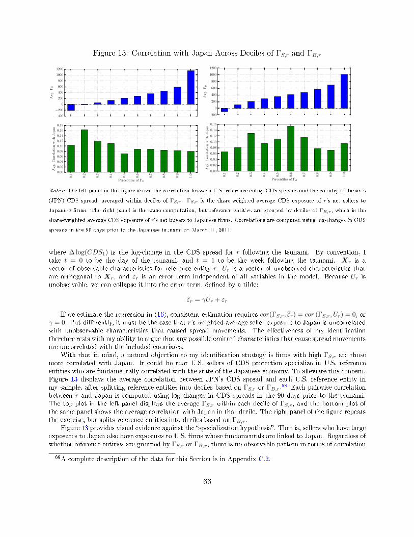
Figure 13: Correlation with Japan Across Deciles of ΓS,r and ΓB,r

−400

−200

0

200

400

600

800

1000

1200

Avg.

ΓS

0.1

0.2

0.3

0.4

0.5

0.6

0.7

0.8

0.9

1.0

Percentiles of ΓS

0.00

0.02

0.04

0.06

0.08

0.10

0.12

0.14

0.16

0.18

Avg.

Cor

rela

tion

wit

hJap

an

−200

0

200

400

600

800

1000

1200

Avg.

ΓB

0.1

0.2

0.3

0.4

0.5

0.6

0.7

0.8

0.9

1.0

Percentiles of ΓB

0.00

0.02

0.04

0.06

0.08

0.10

0.12

0.14

0.16

Avg.

Cor

rela

tion

wit

hJap

an

Notes: The left panel in this �gure shows the correlation between U.S. reference entity CDS spreads and the country of Japan's

(JPN) CDS spread, averaged within deciles of ΓS,r. ΓS,r is the share-weighted average CDS exposure of r's net sellers to

Japanese �rms. The right panel is the same computation, but reference entities are grouped by deciles of ΓB,r, which is the

share-weighted average CDS exposure of r's net buyers to Japanese �rms. Correlations are computed using log-changes in CDS

spreads in the 90 days prior to the Japanese tsunami on March 11, 2011.

where ∆ log(CDS1) is the log-change in the CDS spread for r following the tsunami. By convention, Itake t = 0 to be the day of the tsunami, and t = 1 to be the week following the tsunami. Xr is avector of observable characteristics for reference entity r. Ur is a vector of unobserved characteristics thatare orthogonal to Xr, and εr is an error term independent of all variables in the model. Because Ur isunobservable, we can collapse it into the error term, de�ned by a tilde:

ε̃r = γUr + εr

If we estimate the regression in (16), consistent estimation requires cor(ΓS,r, ε̃r) = cor (ΓS,r, Ur) = 0, orγ = 0. Put di�erently, it must be the case that r's weighted-average seller exposure to Japan is uncorrelatedwith unobservable characteristics that caused spread movements. The e�ectiveness of my identi�cationtherefore rests with my ability to argue that any possible omitted characteristics that cause spread movementsare uncorrelated with the included covariates.

With that in mind, a natural objection to my identi�cation strategy is �rms with high ΓS,r are thosemore correlated with Japan. It could be that U.S. sellers of CDS protection specialize in U.S. referenceentities who are fundamentally correlated with the state of the Japanese economy. To alleviate this concern,Figure 13 displays the average correlation between JPN's CDS spread and each U.S. reference entity inmy sample, after splitting reference entities into deciles based on ΓS,r or ΓB,r.

68 Each pairwise correlationbetween r and Japan is computed using log-changes in CDS spreads in the 90 days prior to the tsunami.The top plot in the left panel displays the average ΓS,r within each decile of ΓS,r, and the bottom plot ofthe same panel shows the average correlation with Japan in that decile. The right panel of the �gure repeatsthe exercise, but splits reference entities into deciles based on ΓB,r.

Figure 13 provides visual evidence against the �specialization hypothesis�. That is, sellers who have largeexposures to Japan also have exposures to U.S. �rms whose fundamentals are linked to Japan. Regardless ofwhether reference entities are grouped by ΓS,r or ΓB,r, there is no observable pattern in terms of correlation

68A complete description of the data for this Section is in Appendix C.2.

66

with Japan. Moreover, the average correlation with Japan within any percentile is relatively low, and neverreaches above 18%.

C.4 Do Observable Reference Entity Characteristics Explain Γi,r?

In addition to explicitly including the aforementioned covariates in my main regression speci�cation, I use twosets of regressions to determine whether observable �rm characteristics can explain cross-sectional variationin ΓS,r and ΓB,r. My identi�cation scheme would suggest this is not the case. Hence, to provide additionalevidence that Γ is orthogonal to unobserved characteristics of U.S. reference entities that caused spreadmovements following the tsunami, I run the following pair of regressions:

Γi,r = a+ β′Xr + εr, i = S,B (17)

where Xr are the full set of control variables. If U.S sellers of protection who had exposure to Japan were�randomly assigned� to U.S. reference entities, then the regression should have very little explanatory power.Table 10 collects these results.

Table 10: Regression of Γ on Reference Entity Observables

Dependent VariableXr ΓS,r ΓB,rρ(r, JPN) -0.28 0.22

(-1.46) (1.17)σCDS 7.57 1.64

(0.93) (0.21)log(NAICS) 0.76 -0.12

(1.33) (-0.23)CDSr(3/11/2011) 0.17 -0.14

(1.46) (-1.24)N 288 288Adj R2 1.9% -0.1%p-value of F -test 0.051 0.45

Notes: The table reports the results of the following regression: Γi,r = a + β′Xr + εr, i = S,B. For example, ΓS,r is the

share-weighted average exposure of r's net sellers to Japanese �rms, where exposure is the net amount of protection sold. Xr is

a vector of observable characteristics of reference entity r: the 90-day trailing correlation of (changes in) r's CDS spread with

the country of Japan's CDS spread, the 90-day trailing volatility of r's CDS spread, the (log) NAICS industry code, and the

level of the CDS spread for r on the day of the tsunami.

Table 10 supports the assumption that U.S. reference entities were �randomly matched� to sellers andbuyers with exposure to Japanese �rms. In both regressions, none of the explanatory variables are statisticallysigni�cant, and the adjusted R2 are near zero. The F -test that all coe�cients in the regression are zerocannot be rejected (barely) at a 5% con�dence interval. In the regressions to come, these results willmanifest themselves when I check whether the e�ect of Γ on CDS spread changes after the inclusion of theaforementioned control variables. Unsurprisingly, adding these controls does not alter the magnitude of myestimated e�ect of Γ on CDS pricing.

67

Figure 14: Correlation with Japan Across Deciles of ΓS,r and ΓB,r

−0.1

0.0

0.1

0.2

0.3

Avg.

Sh

are

0.1

0.2

0.3

0.4

0.5

0.6

0.7

0.8

0.9

1.0

Percentiles of X’s U.S. Share

0.00

0.02

0.04

0.06

0.08

0.10

0.12

0.14

0.16

0.18

Avg.

Cor

rela

tion

wit

hJap

an

Notes: The left panel in this �gure shows the correlation between U.S. reference entity CDS spreads and the country of Japan's

(JPN) CDS spread, averaged within deciles of ΓS,r. ΓS,r is the share-weighted average CDS exposure of r's net sellers to

Japanese �rms. The right panel is the same computation, but reference entities are grouped by deciles of ΓB,r, which is the

share-weighted average CDS exposure of r's net buyers to Japanese �rms. Correlations are computed using log-changes in CDS

spreads in the 90 days prior to the Japanese tsunami on March 11, 2011.

C.5 Does seller J just specialize?

To emphasize the importance of concentration, I explained CDS spread movements after the tsunami usingseller J 's share in each reference entity, denoted by ωJ,r. Recall that seller J had a very large exposure toJapanese �rms prior to the tsunami striking. Like with my use of the Γ variables in the previous subsection,a reasonable objection to this approach is that seller J specializes in U.S. �rms who are fundamentallyconnected. I rule this out in the same way as before. I group U.S. reference entities into deciles based on ωJ,r

and then compute the average correlation with Japan's CDS spread within each decile. Figure (14) displaysthe output of this exercise.

At �rst glance, there does not appear to be a pattern across the deciles of ωJ,r. There is a slight increasein correlation with Japan when moving from the 40th the 50th percentile. However, the absolute magnitudeof the correlation di�erence is small, 10 percent versus 16 percent. To be safe, I have estimated my regressionsonly using reference entities in the 50th percentile and higher. None of my main conclusions are a�ected.I therefore conclude that seller J is not simply specializing in U.S. �rms with fundamental correlation toJapan.

68

D Appendix: Additional Computations Used in the Pa-

per

D.1 Motivating the Benchmark Regression from Reduced Form

Models of Credit Risk

It is standard practice in reduced-form credit risk modeling to view default events as the arrival of a Poissonprocess.69 The Poisson arrival rate is most often called the default intensity or the default arrival rate. Idenote this variable by λMrt , where the superscript M ∈ {Q,P} de�nes either the risk-neutral measure, Q,or the physical measure, P. For illustration, I assume that at each point in time the default intensity isconstant for the remaining life of the CDS position. In this case, the CDS spread of a given reference entitycan be decomposed as:

CDSrt(τ) =λQrt(τ)

λPrt(τ)× LGDQ

rt × λPrt(τ) (18)

where LGDQrt is the loss given default under the risk-neutral measure. The ratio, Πrt := λQrt(τ)/λPrt(τ),

can be interpreted as the default premium for reference entity r. It quanti�es the risk-reward tradeo� forbearing r's default risk.70 A basic tenet of asset pricing is that an asset's risk premium is a combination ofthe quantity of risk and the price of risk. As a rough approximation, suppose that the total default premiumcan be further decomposed by a multiplicative form:

Πrt = QrtΠt

where Qrt is the quantity of risk for r and Πt is the price of credit risk for the entire economy. Standardeconomic logic suggests that the quantity of risk Qrt is high for reference entities that default when marginalutility is high. Suppose further that Qrt = Qr is constant, so that time-variation in the total default premiumis driven only by variation in the price of credit risk Πt.

In this case, taking the log of both sides of Equation (18) gives:

log (CDSrt) = log(LGDQ

rt

)+ log

(λPrt)

+ log(Qr) + log (Πrt) (19)

where I have omitted the functional dependence of variables on the time to maturity. To make Equation(19) empirically operational I need to have estimates of λPrt and LGD

Qrt. Like in Berndt, Douglas, Du�e,

Ferguson, and Schranz (2008), I proxy for λPrt using Moody's 5-year annualized EDF.71

Analogously, I obtain separate estimates of LGDQrt from Markit and Moody's. Denote the choice of

proxy for LGDQrt by L̃GD

Qrt. It is enough to assume that the true LGD is a scalar multiple ηr of the proxy,

69I use the term reduced-form in the spirit of the work by Jarrow and Turnbull (1995), Du�e (1996), andDu�e and Singleton (1999). The popular alternative to this approach are so-called structural models ofcredit, a la Merton (1974).

70Driessen (2002) and Berndt, Douglas, Du�e, Ferguson, and Schranz (2008) provide evidence that, onaverage, Πrt ≈ 1.9. In other words, for every unit of actual default risk taken, the seller of protection mustbe compensated as if she is taking roughly double that amount of default risk.

71Moody's uses observed equity values and volatility to solve for an implicit asset value process. Usingobserved leverage, they translate this to a distance-to-default measure as in Merton (1974). Finally, distance-to-default is mapped to a P-likelihood of default using realized default rates.

69

so LGDQrt = ηrL̃GD

Qrt. In logs, this means:

log(LGDQ

rt

)= log(ηr) + log

(L̃GD

Qrt

)(20)

When might this assumption be reasonable? For instance, the Moody's estimate of LGD is at the sectoral

level. Assuming LGDQrt = ηrL̃GD

Qrt then means a �rm's LGD is a time-invariant scalar transformation of

the sectoral LGD. In other words, time-variation in reference entity LGD is common within a sector, whichseems plausible.72

Substituting Equation (19) into Equation (20) yields:

log (CDSrt) = log(ηr) + log(Qr) + log

(L̃GD

Qrt

)+ log

(λPrt)

+ log (Πt) (21)

Equation (21) is a panel regression, in logs, of CDS spreads on a reference entity �xed e�ect, plus proxiesfor the risk-neutral LGD and the physical default intensity. The reference entity �xed e�ects absorbs boththe �rm-speci�c component of LGD, ηr, and the comovement of r with marginal utility, Qr. After controllingfor �rm speci�c variables, Equation (21) suggests the additional control variables that enter the regressioncapture the price of credit risk, Πt.

This interpretation rests crucially on the link between CDS and bond markets. It could very well bethe case that �uctuations in CDS spreads are not accompanied by variation in bond yields. That is, if Iobserve CDS spreads changing, it may be the CDS-bond basis � loosely speaking the di�erence betweenCDS spreads and bond spreads � is actually what is moving around. In theory, the CDS-bond basis shouldbe zero, but there is a substantial amount of empirical evidence to suggest that this is not always the case.73

In Appendix B, I use actual bond yields to con�rm my results do indeed pertain to the price of credit risk,as opposed to the CDS-bond basis. Finally, Equation (21) suggests one can estimate Πt using a referenceentity controls plus a time �xed e�ect, which I implement in the next section.

D.2 A Panel Estimate of the Price of Aggregate Credit Risk

Motivated by the analysis in the previous section, I estimate the price of credit risk by running the followingregression:

log (CDSrt) = c+ ar + β1 log (EDFrt) + β2 log

(L̃GD

Qrt

)+ πt + εrt (22)

where ar is a reference entity �xed e�ect and πt is a time �xed e�ect. To recover the price of risk at anypoint in time, I simply exponentiate the time-�xed e�ect:

Π̂t = exp (π̂t) (23)

where the standard error of Π̂t is computed using the Delta method.74 Crucially, my price of risk estimateat each point in time is a relative estimate. That is, Π̂t is the ratio of the price of risk at time t to the priceof risk on the �rst day of the sample, which for this portion of the paper is 2/19/2014. The reason this isthe case is simply because estimation via the time �xed e�ect cannot separately identify the price of risk for

72When L̃GDQrt comes from Markit, L̃GD

Qrt is provided for each reference entity (as opposed to each

sector). In this case, the assumption says the Markit's estimate of LGD is potentially biased in a time-invariant way. For example, if ηr = 1.1, then I am assuming Markit's LGD for r are always 10% higher thanreality. Of course, nothing in my approach restricts ηr from being one.

73For example, Bai and Collin-Dufresne (2013).74i.e. the standard error for Π̂t is exp(πt)× se(πt).

70

the �rst day in the sample from the �xed e�ect of the �rst �rm.75 Even though I am unable to pinpoint theexact level of the price of risk, it is enough for my purposes to study the relative level of the price of risk.

Next, I present the results of the simple panel regression:

log(CDSrt) = 0.60 + 0.25 log(EDFrt) + 0.36 log

(L̃GD

Qrt

)+

∑r ar1r +

∑t πt1t

(32.4) (9.9) (4.8)(24)

where the t-statistics are listed below estimated coe�cient values. All t-statistics are computed by clusteringwithin each reference entity and time.

A similar approach is taken by Gilchrist and Zakrajsek (2012) to estimate what they call the �excessbond premium�. However, instead of estimating Πt using a time-�xed e�ect, they �rst obtain the �tted(level) of CDS spreads from the panel regression. Next, they compute �residuals� as the di�erence betweenactual credit spread levels and this �tted variable, along with a Jenson volatility correction. Finally, theirexcess bond premium in each period is the average residual across all bonds.

My time �xed-e�ect methodology is a simpli�cation of this procedure. Recall that I motivated thetime �xed e�ect estimator of Πt from the stylized reduced form model of credit in the previous subsection;however, the validity of my estimate of Πt is not anchored to the assumptions in that model. Alternatively,Πt can be interpreted from a purely statistical perspective; it computes within-period averages of the portionof CDS spreads not captured by �rm-fundamentals. This is the strictest sense in which I view Πt as highlyrelated to Gilchrist and Zakrajsek's (2012) excess bond premium.

D.3 Appendix: Using Mark-to-Market Losses to Compute CDS

Portfolio Returns

D.3.1 Portfolio Return of a Single Counterparty

Let me start with a simpler question: what is the annualized return, from the perspective of a seller, of asingle position? Suppose the position was initiated at time zero, so that the change in the mark to marketvalue at time t is denoted by V p

c,t. The p superscript denotes that this is the value of a single position, p.As a matter of convention, V p

c,t is computed from the perspective of a seller. Thus, if c is a buyer in theposition, the contribution of the position to her overall portfolio is −V p

c,t.To answer the question, one must make an important assumption on the leverage allowed in the position.

If the notional of the position is Npc,t, then zero leverage indicates that the seller of protection must post the

full value of Npc,t into an initial margin account at time zero. The zero leverage assumption has been made

by previous studies such as Bao and Pan (2012), Berndt and Obreja (2010), and Junge and Trolle (2014).For generality, I assume that the seller of protection must post l ∈ (0, 1] of the total notional as an initialmargin. If at time t, the position is unwound, the annualized return is computed by looking at the cash�ows:

Rpc,t =

1

τpt×(lNp

c,t + V pc,t +AP p

c,t

)− lNp

c,t

lNpc,t

=1

τpt× V p

c,t + +AP pc,t

lNpc,t

where τpt is the time that has elapsed, in years for the position. In this example, τpt = t. AP pc,t is the accrued

75This is one major advantage of the approach in BDDFS, who estimate a process for λQt and λPt directly.As such, they can compute the price of risk (e.g. the ratio) at each point in time. Even in this case, theymust determine the initial condition for each process in order to determine the level of the default intensities.This initialization comes from the parameters of the underlying processes.

71

premium, from the perspective of the seller, of the position.At time t, the seller of protection receives back her initial margin of lNp

c,t, plus the proceeds of Vpc,t from

unwinding the position and any accrued premiums.76 Her initial investment was lNpc,t, and scaling by 1/τpt

puts the return in annualized terms.The issue of the correct leverage, l, is important. It is generally di�cult to observe, and for the trans-

actions in my dataset it seems to be poorly measured.77 To make matters worse, it seems that leverage isheterogeneous even across the positions of a single counterparty. This makes sense, as bargaining power willcertainly play a role in the amount of leverage that one side of the swap can take.

In the absence of better data, I must make some additional assumptions in order to proceed. For theremainder of the paper, I assume that l = 1 for all counterparties. This is undoubtedly too simpli�ed, as itseems natural that di�erent counterparty types will be allowed to take di�erent leverage. For robustness, Ireplicate all of the results in this section using dollar changes in portfolio value in the Online Appendix. Thisapproach does not su�er from the aforementioned caveats, but does make interpretation slightly di�erentsince there is great deal of heterogeneity in the trading volumes of di�erent counterparties in the market,not to mention the issue of annualizing gains.

Under the assumption of l = 1, the total annualized return of a counterparty's portfolio is just theweighted average of the returns of each position, weighted by the gross size of the position:

Rc,t =∑

p∈Pt(c)

Npc,t∑

p∈Pt(c)

Npc,t

Rpc,t

=

∑p∈Pt(c)

(V pc,t +AP p

c,t

)/τpt∑

p∈Pt(c)

Npc,t

(25)

where Pt(c) is the set of counterparty c's positions as of time t.

D.3.2 Portfolio Return of Top Five Sellers and Buyers

Denote the aggregate top �ve buyers by TABt for �top aggregate buyers�. TASt is the top �ve aggregatesellers. I treat each group as a single trader, and compute the total annualized CDS portfolio return. Theseare my measures of the risk bearing capacity of mega-sellers and mega-buyers. Formally, this means:

RBst :=

∑c∈TASt

[∑p∈Pt−1(c)

(V pc,t−1 +AP p

c,t−1)/τpt−1

]∑

c∈TASt

[∑p∈Pt−1(c)

Npc,t−1

]RBb

t :=

∑c∈TABt

[∑p∈Pt−1(c)

(V pc,t−1 +AP p

c,t−1)/τpt−1

]∑

c∈TABt

[∑p∈Pt−1(c)

Npc,t−1

] (26)

D.4 Option Implied CDS Spreads

This section describes how I use American option prices to compute an implied CDS spread. For a completetheoretical treatment of this procedure, see Carr and Wu (2013), henceforth CW. In the interest of space, I

76Implicitly, this assumes that the initial margin account earns zero interest. This can be easily relaxed.77See a recent paper by Du�e, Scheicher, and Vuillemey (2014) for a more detailed discussion of initial

margining.

72

present only the relevant formulas and data descriptors used in the main text.To start, Carr and Wu (2013) de�ne what they call a �unit recovery claim� that pays a dollar if there is

a default event prior to an option's expiration, and zero otherwise. CW assume that there exists a defaultcorridor [A,B] that the underlying equity price can never enter. If the equity price hits the level B, there isa default and the stock price immediately jumps to a level that is bounded above by A. In their empiricalwork, they set A = 0, which means that the equity value drops to zero upon default. I continue with thisassumption for the remainder of my treatment.

Under this assumption, CW show that, regardless of the underlying asset process, there is a robust linkbetween the unit recovery claim and CDS spreads on the underlying �rm. The unit recovery claim is de�nedas follows:

UO(t, T ) =Pt(K2, T )− P (K1, T )

K2 −K1(27)

where A ≤ K1 < K2 ≤ B. It is easy to see that, under the assumptions of the default corridor, this paysone dollar if there is default and zero otherwise.

Next, CW show that under the assumption of a constant arrival rate and constant interest rate, the CDSspread of a �rm is related to the price of the unit recovery claim in the following manner:

UO(t, T ) = ξk × 1− exp (−(r + ξk)(T − t))r(t, T ) + ξk

(28)

where ξ = 1/(1 − R), R is the recovery of the bond upon default, k is the CDS spread, and r(t, T ) is thecontinously compounded interest rate between t and T . Here, T is meant to capture the expiration of boththe CDS contract and the option contract. For my purposes, I will always set T − t = 5.

Equation (28) provides a simple way to recover a CDS spread implied by option prices. Using observedoption prices, one �rst computes the value of the unit recovery claim. A simple numerical inversion thendelivers the implied CDS spread.

To implement this procedure in practice, I merge my panel of CDS spreads with American option pricesfrom OptionsMetrics using 6 digit CUSIPs. Furthermore, since I follow CW in assuming A = 0, the unitrecovery claim is simple the price of a deep out of the money put option, divided by its own strike price. Iuse a set of �lters on the options data that is similar to CW: (i) I take the option price to be the midpointof the bid and o�er; (ii) I consider options whose bid is strictly positive; (iii) I consider options whose openinterest is strictly positive; (iv) the maturity of the option must be greater than 365 days; (iv) I use the putoption that satis�es all of the preceding qualities, and that has the delta closest to 0 and less than -0.15.

Naturally, there is a maturity mismatch in using options that might have an expiration of 2 yearsto compute an implied CDS spread of 5 years. There is no real way to avoid this bias. See CW for aricher discussion. Like with other portions of the paper, the riskfree rate is obtained from interpolating theUSD swap rate curve. Finally, I use the Markit reported recovery rate, which has the added advantage ofmaintaining consistency with the benchmark panel regression in the main text.

73