COMSOL LEP tutorial for Startup of a CSTR (Chapter-13)

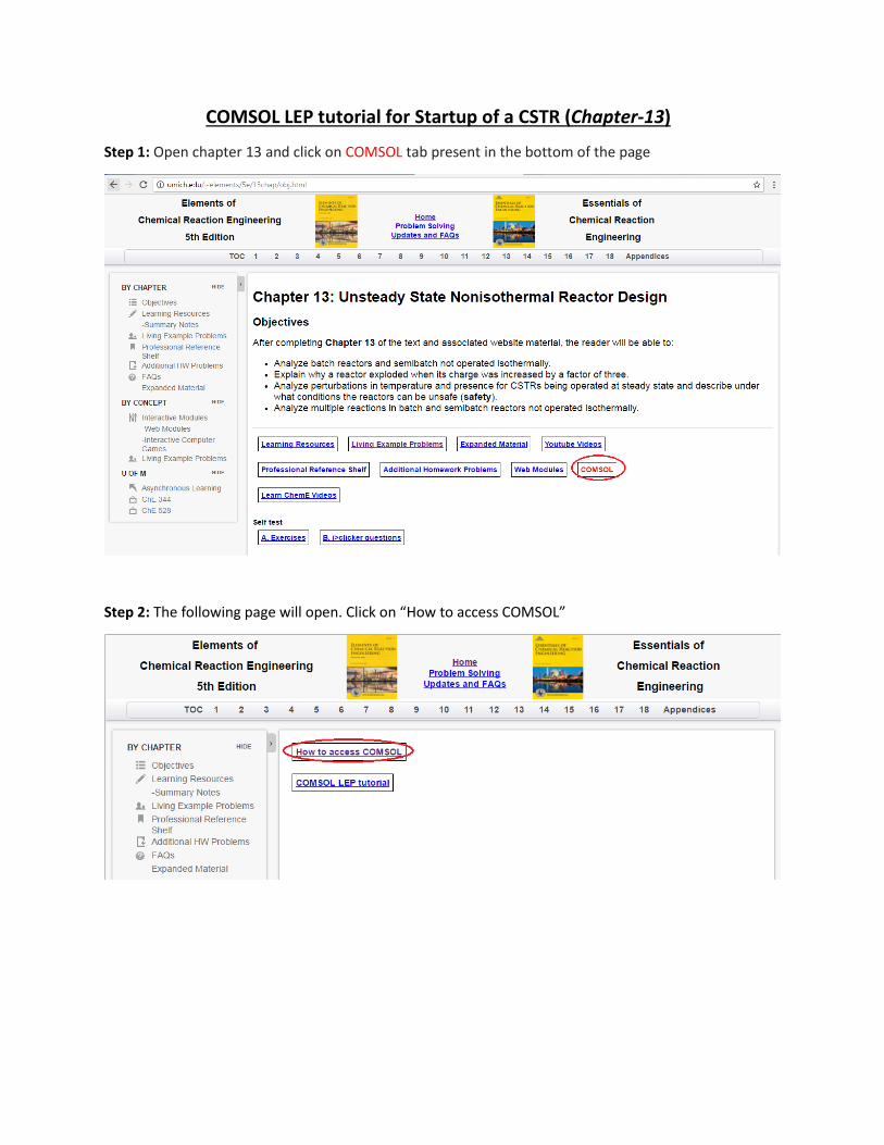
Step 1: Open chapter 13 and click on COMSOL tab present in the bottom of the page

Step 2: The following page will open. Click on “How to access COMSOL”

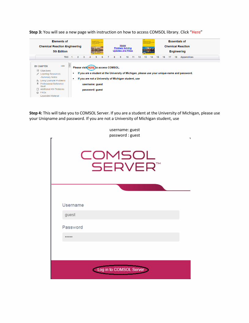
Step 3: You will see a new page with instruction on how to access COMSOL library. Click “Here”

Step 4: This will take you to COMSOL Server. If you are a student at the University of Michigan, please use your Uniqname and password. If you are not a University of Michigan student, use

username: guest password : guest

Step 5: This will open up COMSOL library where you can see many COMSOL files to solve chemical reaction

engineering problems. Find “Startup of a CSTR Part-1”. Click on “Run in browser” to start the application

You will see that following window opens which has input parameters, description, graphical features

(Concentration and Temperature profiles) and a few buttons. Currently Concentration profile is visible.

Step 6: Click on Temperature tab to view Temperature profile

Step 7: Under Input section on the left hand side, you can view and change any parameter values. Let’s

change a parameter and see the effect on the profile. Change the Initial reactor temperature from 340 K

to 310 K. After you are done, click on Compute button ( ) present above the Input parameters

Caution: The y axis is dynamic and scale changes with respect to the values. Make sure to look at both

scale and graph

Step 8: Now check the Concentration and Temperature profiles. The following graphs will be obtained.

You can check that the concentration profile now has more oscillations before reaching steady state

The following is the temperature profile that you will obtain. You can see that at lower temperature, it

takes more time to reach the steady state value

Step 9: Now if you want to re-set all the parameter values to its initial values, click on “Reset to Default

button( ) present on the menu bar . Click on this button to reset the value of Temperature. To update

the graph, click on Compute button. Each time you change a variable, click Compute

Step 10: Now let’s consider a case where there is no coolant flow. Enter the Cooling fluid molar flow rate

to be 0 mol/s and click compute to see its effect on profile

The following graph will be obtained for Concentration profile. You can see that reactant concentration

drops instantaneously without coolant flow

Following is the temperature profile you will obtain. It can be seen that temperature also rises suddenly

without coolant flow

Step 11: Now, you can change any listed parameter value and check its effect on profiles. Make sure to

click Compute button after you change a variable.

Step 12: If you have COMSOL installed on your computer, then you can also download the complete

COMSOL file (with user interface)

a) Go to file on toolbar and click on Save button. This will download the file at the bottom of the

browser (if you are using Chrome)

b) Click on the downloaded file to open the application

Step 13: You can also open a pdf documentation which details the reactor model and a step-by-step-

procedure to create this COMSOL module from scratch. Click on PDF button present on the menu bar

This will open up a new tab with PDF file which you can also download

Step 14: Now go back to Library and Find “Startup of a CSTR- Part 2”. Click on “Run in browser” to start

the application. This application contains parametric graph of Concentration vs Temperature

The application will look like this when it opens. Again you can see that there are Input parameters,

buttons and graphs. Currently the graph shows parametric plot of Concentration vs Temperature at

different initial values of PrO concentration and Reactor temperature

Step 15: Click on “Temperature vs Time” tab to obtain Temperature profile at different initial conditions

of PrO concentration and Reactor temperature

Step 16: Let’s change a parameter and see the effect on the profile. Suppose Practical stability limit is 350

K and you want to size the reactor so that maximum reactor temperature is below this limit. Change the

Tank volume to 0.8 m3 from 1.89 m3. After you are done, click on Compute button ( ) present above the

Input parameters

Caution: The y axis is dynamic and scale changes with respect to the values. Make sure to look at both

scale and graph

The following graph will be obtained for “Concentration vs Temperature”. It can be seen that reactor

temperature doesn’t cross the Practical stability limit at Tank volume=0.8 m3

Step 17: Now let’s change another variable and see the effect on profiles. Change the feed stream

temperature to 350 K from its initial value of 289 K and then click Compute

The following graph will be obtained for Concentration vs Temperature

The following graph will be obtained for Temperature vs Time

Step 18: Again, you can download the COMSOL file as was shown in Step 12. To open PDF documentation

to view the detail of the COMSOL modeling steps, click on PDF button as shown below

This will open up a new tab with PDF file which you can download also