COMPUTING THE SMITH FORMS OF INTEGER MATRICES

AND SOLVING RELATED PROBLEMS

by

Zhendong Wan

A dissertation submitted to the Faculty of the University of Delaware in partialfulfillment of the requirements for the degree of Doctor of Philosophy in Computer Sci-ence

Summer 2005

c© 2005 Zhendong WanAll Rights Reserved

COMPUTING THE SMITH FORMS OF INTEGER MATRICES

AND SOLVING RELATED PROBLEMS

by

Zhendong Wan

Approved:Henry R. Glyde, Ph.D.Interim Chair of the Department of Computer and Information Sciences

Approved:Thomas M. Apple, Ph.D.Dean of the College of Arts and Sciences

Approved:Conrado M. Gempesaw II, Ph.D.Vice Provost for Academic and International Programs

I certify that I have read this dissertation and that in my opinion it meets theacademic and professional standard required by the University as a dissertationfor the degree of Doctor of Philosophy.

Signed:B. David Saunders, Ph.D.Professor in charge of dissertation

I certify that I have read this dissertation and that in my opinion it meets theacademic and professional standard required by the University as a dissertationfor the degree of Doctor of Philosophy.

Signed:John Case, Ph.D.Member of dissertation committee

I certify that I have read this dissertation and that in my opinion it meets theacademic and professional standard required by the University as a dissertationfor the degree of Doctor of Philosophy.

Signed:Bob Caviness, Ph.D.Member of dissertation committee

I certify that I have read this dissertation and that in my opinion it meets theacademic and professional standard required by the University as a dissertationfor the degree of Doctor of Philosophy.

Signed:Erich Kaltofen, Ph.D.Member of dissertation committee

I certify that I have read this dissertation and that in my opinion it meets theacademic and professional standard required by the University as a dissertationfor the degree of Doctor of Philosophy.

Signed:Qing Xiang, Ph.D.Member of dissertation committee

ACKNOWLEDGEMENTS

I would like to express my sincere gratitude to those who have guided, encouraged,

and helped me during my Ph.D. study.

First, I would like to thank my Ph.D thesis adviser, Prof. B. David Saunders, for

his guiding and encouragement. This thesis could not be done without his guiding and

encouragement.

I would like to thank Mrs. Nancy Saunders for her encouragement and hospitality,

thank all committee members, Prof. John Case, Prof. Bob Caviness, Prof. Erich Kaltofen,

and Prof. Qing Xiang, for their guiding, encouragement, and help.

I would like to thank my friends for all kinds of help. Especially thank all linbox

members for their encouragement and help, thank Mr. Leon La Spina and Mr. Danial

Rochel for reading my thesis and correcting my writing.

Finally, I would like to thank my wife, Fei Chen (Mrs. Wan), for her patience,

encouragement, and help with my English. Also, I would like to thank my parents, brother

and sister for their support.

iv

TABLE OF CONTENTS

LIST OF FIGURES . . . . . . . . . . . . . . . . . . . . . . . . . . . . . . . . viiiLIST OF TABLES . . . . . . . . . . . . . . . . . . . . . . . . . . . . . . . . . ixABSTRACT . . . . . . . . . . . . . . . . . . . . . . . . . . . . . . . . . . . . . x

Chapter

1 INTRODUCTION . . . . . . . . . . . . . . . . . . . . . . . . . . . . . . . 12 COMPUTATION OF MINIMAL AND CHARACTERISTIC

POLYNOMIALS . . . . . . . . . . . . . . . . . . . . . . . . . . . . . . . . 8

2.1 Introduction . . . . . . . . . . . . . . . . . . . . . . . . . . . . . . . . 82.2 Minimal polynomials over a finite field. . . . . . . . . . . . . . . . . . 9

2.2.1 Wiedemann’s method for minimal polynomial. . . . . . . . . . 92.2.2 An elimination based minimal polynomial algorithm. . . . . . . 12

2.3 Characteristic polynomials over a finite field. . . . . . . . . . . . . . . . 13

2.3.1 A blackbox method. . . . . . . . . . . . . . . . . . . . . . . . 142.3.2 Two elimination based methods. . . . . . . . . . . . . . . . . . 152.3.3 LU-Krylov method for characteristic polynomial. . . . . . . . . 162.3.4 Experiments: LU-Krylov vs. Keller-Gehrig. . . . . . . . . . . . 18

2.4 Minimal and characteristic polynomials over the integers. . . . . . . . . 202.5 An application . . . . . . . . . . . . . . . . . . . . . . . . . . . . . . . 24

3 COMPUTATION OF THE RANK OF A MATRIX . . . . . . . . . . . . . 25

3.1 Introduction . . . . . . . . . . . . . . . . . . . . . . . . . . . . . . . . 253.2 Wiedemann’s algorithm for rank. . . . . . . . . . . . . . . . . . . . . . 263.3 GSLU: a sparse elimination. . . . . . . . . . . . . . . . . . . . . . . . 28

v

3.4 Complexity comparison. . . . . . . . . . . . . . . . . . . . . . . . . . 293.5 An adaptive algorithm. . . . . . . . . . . . . . . . . . . . . . . . . . . 303.6 Experimental results. . . . . . . . . . . . . . . . . . . . . . . . . . . . 31

4 COMPUTATION OF EXACT RATIONAL SOLUTIONS FOR LINEARSYSTEMS . . . . . . . . . . . . . . . . . . . . . . . . . . . . . . . . . . . 33

4.1 Introduction . . . . . . . . . . . . . . . . . . . . . . . . . . . . . . . . 334.2 p-adic lifting for exact solutions. . . . . . . . . . . . . . . . . . . . . . 344.3 Using numerical methods. . . . . . . . . . . . . . . . . . . . . . . . . 354.4 Continued fractions. . . . . . . . . . . . . . . . . . . . . . . . . . . . 374.5 Exact solutions of integer linear systems. . . . . . . . . . . . . . . . . . 40

4.5.1 An exact rational solver for dense integer linear systems. . . . . 41

4.5.1.1 Total cost for well-conditioned matrices. . . . . . . . 464.5.1.2 Experimentation on dense linear systems. . . . . . . . 47

4.5.2 An exact rational solver for sparse integer linear systems. . . . . 48

4.6 An application to a challenge problem. . . . . . . . . . . . . . . . . . . 494.7 An adaptive algorithm. . . . . . . . . . . . . . . . . . . . . . . . . . . 51

5 COMPUTATION OF SMITH FORMS OF INTEGER MATRICES . . . . 53

5.1 Introduction . . . . . . . . . . . . . . . . . . . . . . . . . . . . . . . . 535.2 The definition of Smith form. . . . . . . . . . . . . . . . . . . . . . . . 545.3 Kannan and Bachem’s algorithm. . . . . . . . . . . . . . . . . . . . . . 565.4 Iliopoulos’ algorithm. . . . . . . . . . . . . . . . . . . . . . . . . . . . 605.5 Storjohann’s near optimal algorithm. . . . . . . . . . . . . . . . . . . . 635.6 Eberly, Giesbrecht, and Villard’s algorithm with improvements. . . . . . 67

5.6.1 Largest invariant factor with a “bonus” idea. . . . . . . . . . . . 685.6.2 The invariant factor of any index with a new efficient perturbation 70

5.6.2.1 Non-uniformly distributed random variables. . . . . . 72

vi

5.6.2.2 Proof of Theorem 5.8. . . . . . . . . . . . . . . . . . 81

5.6.3 Binary search for invariant factors. . . . . . . . . . . . . . . . . 82

5.7 Smith form algorithms for sparse matrices. . . . . . . . . . . . . . . . . 83

5.7.1 Smith forms of diagonal matrices. . . . . . . . . . . . . . . . . 84

5.8 An adaptive algorithm for Smith form. . . . . . . . . . . . . . . . . . . 875.9 Experimental results. . . . . . . . . . . . . . . . . . . . . . . . . . . . 92

BIBLIOGRAPHY . . . . . . . . . . . . . . . . . . . . . . . . . . . . . . . . . 97

vii

LIST OF FIGURES

2.1 The principle of computation of the minimal polynomial. . . . . . . . 12

2.2 Diagram for Keller-Gehrig’s algorithm. . . . . . . . . . . . . . . . . 16

2.3 Over random matrices. . . . . . . . . . . . . . . . . . . . . . . . . . 19

2.4 Over matrices with rich structures. . . . . . . . . . . . . . . . . . . . 19

3.1 Blackbox VS GSLU over random dense matrices. . . . . . . . . . . . 29

3.2 Experimental result of adaptive algorithm. . . . . . . . . . . . . . . . 32

5.1 A gcd/lcm sorting network . . . . . . . . . . . . . . . . . . . . . . . 85

5.2 Diagonal matrix Smith form speedup (classical method time / sortingnetwork time). . . . . . . . . . . . . . . . . . . . . . . . . . . . . . . 87

5.3 An engineered algorithm to compute the Smith form.. . . . . . . . . 89

viii

LIST OF TABLES

4.1 Run time of different algorithms for exact solutions. . . . . . . . . . . 47

4.2 Comparison of different methods for solving a challenge problem. . . 51

5.1 Algorithms for computing Smith forms. . . . . . . . . . . . . . . . . 87

5.2 Run time of our engineered algorithm on constructed examples. . . . . 93

5.3 Run time of our engineered algorithm over practical examples. . . . . 95

ix

ABSTRACT

The Smith form of an integer matrix plays an important role in the study of alge-

braic group theory, homology group theory, systems theory, matrix equivalence, Diophan-

tine systems, and control theory. Asymptotic complexity of the Smith form computation

has been steadily improved in the past four decades. A group of algorithms for computing

the Smith forms is available now. The best asymptotic algorithm may not always yield

the best practical run time. In spite of their different asymptotic complexities, different

algorithms are favorable to different matrices in practice. In this thesis, we design an

algorithm for the efficient computation of Smith forms of integer matrices. With the com-

puting powers of current computer hardware, it is feasible to compute the Smith forms of

integer matrices with dimension in the thousands, even ten thousand.

Our new “engineered” algorithm is designed to attempt to combine the best aspects

of previously known algorithms to yield the best practical run time for any given matrix

over the integers. The adjective “engineered” is used to suggest that the structure of

the algorithm is based on both previous experiments and the asymptotic complexity. In

this thesis, we also present lots of improvements for solving related problems such as

determining the rank of a matrix, computing the minimal and characteristic polynomials

of a matrix, and finding the exact rational solution of a non-singular linear system with

integer coefficients.

x

Chapter 1

INTRODUCTION

Number systems provide us the basic quantitative analysis tool to understand the

world and predict the future, and algebra is the abstract study of number systems and

operations within them. Computer algebra which designs, analyzes, implements and ap-

plies algebraic algorithms has risen as an inter-disciplinary study of algebra and computer

science. The power of computers has increased as predicted by Moore’s law. Thus sym-

bolic (exact) computation has become more and more important. Symbolic computation,

which is often expensive in computation time, delivers the answer without any error, in

contrast to numerical linear algebra computation.

In my thesis, I address the efficient computation of the Smith normal form (Smith

form, in short) of a matrix over the integers, a specific problem in computer algebra.

I will also address some related problems, including computing the matrix rank, exactly

solving integer linear systems, and computing the minimal and characteristic polynomials

of a matrix. For ann × n integer matrix, the number of non-zero diagonal entries of the

Smith normal form is equal to the rank of the matrix and the Smith form of the matrix

can be obtained by computing O∼(log n) characteristic polynomials or by exactly solving

O∼(√

n) linear systems (usually with integer coefficients). In each chapter, I discuss each

problem in detail.

My main contribution to computer algebra can be summarized as follows:

1. Algorithms with good asymptotic complexity may not be efficient in practice. In

order to achieve high performance, it is necessary to optimize them from a practical

1

point of view. A high performance package needs both good algorithms and good

implementations. There are many different Smith form algorithms. If asymptotic

complexity is used as the only criteria to compare them, it is easy to sort these

algorithms. But in practice, it’s hard to tell which is best. Asymptotically best algo-

rithms may not always yield the best practical run time. Each algorithm may yield

the fastest run time for certain cases. We have developed an “engineered” algorithm

that attempts to utilize the best aspects of the previous known methods. We called

it “engineered” because its structure is based on both theoretical and experimental

results. In particular, we discovered the importance of separating the rough part

and smooth part of invariant factors. Different algorithms are suitable for different

parts. Thus we could divide the problem into two sub-problems of computing the

rough part and the smooth part. For each subproblem, we used adaptive algorithms

to solve it based on thresholds, which are determined by both theoretical and ex-

perimental results. We implemented the engineered algorithm in LinBox, which is

accessible atwww.linalg.org . Experiments showed significant success. The

engineered algorithm yields the nearly best practical run time for all cases, and

guarantees the worst case asymptotic complexity of the Smith normal form algo-

rithm [EGV00]. A preliminary version of the engineered Smith form algorithm was

discussed in our paper [SW04]. A more complete version is planned. Details can

also be found in chapter 5

2. In [EGV00], the Smith normal form computation of an integer matrix can be re-

duced to solvingO∼(√

n) integer linear systems of dimensionn × n. For a non-

singularn × n integer matrixA and a randomly chosen integer vectorb, the least

common multiple of all denominators of the solution of the linear equationAx = b

is very likely to be equal to the largest invariant factor (the largest diagonal entry

of the Smith normal form) Using perturbation matricesU andV , whereU is an

n× i integer matrix andV is ani× n integer matrix, the largest invariant factor of

2

A + UV is very likely to be theith invariant factor ofA (the ith diagonal entry of

the Smith form ofA). For this perturbation, a number of repetitions are required

to achieve a high probability of correctly computing theith invariant factor. Each

distinct invariant factor can be found through a binary search. We have proven that

the probability of success in computing theith invariant factor is better than pre-

viously known results, thereby allowing the resulting algorithm to terminate after

fewer steps. We also improved the preconditioning process by the following: We

replaced the additive preconditioner by a multiplicative preconditioner. Namely, to

compute theith invariant factor we show that the preconditioner[Ii, U ] and[Ii, V ]T

(U is ani×(n−i) random integer matrix andV is an(n−i)×i random integer ma-

trix) is sufficient and is more efficient because the resulting system is(n−i)×(n−i)

rather thann× n. Details can be found both in chapter 5 and in [SW04].

3. Finding the rational solution to a non-singular system with integer coefficients is a

classical problem. Many other linear algebra problems can be solved via rational

solutions.p-adic lifting [MC79, Dix82] yields the best asymptotic complexity for

exactly solving integer linear systems. Numerical linear methods often deliver ap-

proximate solutions but much faster than exact linear algebra methods. Many high

performance tools have been developed, for example the BLAS (Basic Linear Alge-

bra Subprograms) implementations []. In order to get an approximate solution with

high accuracy, numerical methods such as in [GZ02] depend on high precision soft-

ware floating point operations. that are expensive in both asymptotic and practical

run time costs. Using floating point machine arithmetic, BLAS can quickly deliver

a solution accurately up to a few bits in a well-conditioned case. In practice, integer

matrices are often well-conditioned. It is well known that numeric methods can

quickly deliver the solution accurately up to a few bits in well-conditioned cases.

In practice, we often meet well-conditioned cases. For a well-conditioned case, we

found that by the repeated use of the BLAS to compute low precision approximate

3

solutions to linear systems that are amplified and adjusted at each iteration, we can

quickly compute an approximate solution to the original linear system to any de-

sired accuracy. We show how an exact rational solution can be constructed with a

final step after a sufficiently accurate solution has been completed with the BLAS.

The algorithm has the same asymptotic complexity asp-adic lifting. Experiment

results have shown significant speedups. Details can be found both in chapter 4 and

in [Wan04].

4. In linear algebra, many problems such as finding the rational solution of a non-

singular integer linear system and computing the characteristic polynomial of an

integer matrix are solved via the modular methods. The answer is a vector of in-

tegers or a vector of rationals. Working with a single prime via Hensel lifting or

with many different primes via the Chinese remainder algorithm is the common

way to find the solution modulo a large integer. A priori bounds like Hadamard’s

bound for the solution of a linear system can be used to determine a termination

bound for the Hensel or the Chinese remainder method, that is when the power of

the single prime in the Hensel method or the product of the primes in the Chinese

remainder method meets or exceeds the termination bound, the exact solution over

the integers or rationals, as appropriate, can be constructed. But in practice, the

exact solution can often be constructed before the termination bound is met. If the

modulus answers are the same for two contiguous iterations of the Hensel or the

Chinese remainder method, then it is highly likely that the exact desired result can

be constructed at this point thereby yielding an efficient probabilistic algorithm that

eliminates the need for additional repetitions to reach the a priori termination bound

of the deterministic method. - see e.g [BEPP99, Ebe03]. However, computing all

the entries of a solution vector at each step in the Hensel or the Chinese remainder

method is quite expensive. We have developed a new method - at each step, only

a single number instead of a vector of numbers is reconstructed to decide if more

4

steps are needed. The number, which is called the ”certificate”, is a random lin-

ear combination of the entries of the modular answer. With high probability, when

an early termination condition is met, the exact solution can be constructed from

the modular answer at this point. Details can be found both in chapter 2 and in

[ASW05].

5. The rank of an integer matrix can be found via computation modulo one or more

random primes. The computation of the rank of a matrix over a finite field can

be done by elimination or by a black box method. With preconditioners as in

[EK97, KS91, CEK+02], it most likely has no nilpotent blocks of size greater than1

in its Jordan canonical form and its characteristic polynomial charpoly(x) is likely

to be equal to its minimal polynomial except missing a factor of a power ofx. If a

matrix has no nilpotent blocks of size greater than one in its Jordan canonical form,

then its rank can be obtained from its characteristic polynomial. Since in this case,

the multiplicity of the roots in its characteristic polynomial is equal to the dimen-

sion of its null space and the rank is equal to the difference of its dimension and the

dimension of its null space. For a large sparse system, a sparse elimination method

which tries to minimize the fill-in can be very efficient in practice. A version of

SuperLU [Sup03] over the finite fields is very efficient in practice - see [DSW03].

Also a blackbox method can be used to efficiently determine the rank. Each method

is better for certain cases. Which to use in practice is hard to answer. We found

an adaptive algorithm that starts an elimination first, and switches to a blackbox

method if it detects a quick rate of fill-in. This adaptive algorithm turns out to be

efficient in practice. Experimental results have shown that the run time of the adap-

tive algorithm is always close to the minimum run time of the two. The approach

can be easily adopted to other linear problems such as computing the determinant.

Details can be found both in chapter 3 and in [DSW03, LSW03].

6. I have implemented my algorithm in the LinBox library, a C++ template library

5

for exact, high-performance linear algebra computation. I have improved the Lin-

Box interface design and data structures for sparse matrices, improved the previous

implementations, and added many functionalities. All my algorithms I have dis-

cussed above are available in LinBox. The beta version is available athttp:

//www.linalg.org .

The thesis consists of four parts. Each part addresses a different problem and dis-

cusses the history of the problem and my contributions. In each part, I present different

methods for the sparse and dense cases. Due to memory efficiency, even run time effi-

ciency, it is often not a good idea to treat large sparse cases just like dense cases. There

are many good algorithms for sparse cases of different problems. I start with the prob-

lem of computing the characteristic and the minimal polynomials. Two distinct methods

for computing a minimal polynomial over a finite field are presented. One is Wiede-

mann’s method [Wie86], which is better for sparse matrices. The other is the Krylov

subspace based elimination which is favorable to dense matrices. Wiedemann’s method

can be adopted to determine the rank of a matrix and the two methods can be adopted to

compute the valence, which will be introduced in the chapter about Smith forms. Charac-

teristic polynomials can be computed based on the corresponding minimal polynomials.

Computation of minimal and characteristic polynomials over the integers cases are also

discussed. Then the matrix rank problem is addressed. For an integer matrix, its rank

gives information about the number of non-zeroes invariant factors. The rank of an in-

teger matrix can be found via computation modulo random primes. Over a finite field,

(sparse) elimination can be used to determine the rank. For a sparse matrix over a finite

field, Wiedemann’s method with good preconditioners as in [EK97, KS91, CEK+02] can

determine the rank efficiently in practice. Sparse elimination and Wiedemann’s method

are favored by different cases. Also a practically efficient adaptive algorithm based on

the two methods is presented. After that, exact rational solutions of non-singular linear

systems are discussed. Exact rational solutions of non-singular linear systems can be

6

used to determine the largest invariant factors of integer matrices. With perturbation as

in [EGV00, SW04], exact rational solutions can also be used determine any indexed in-

variant factors.p-adic lifting [MC79, Dix82] is a common way to find exact solutions of

non-singular linear systems. In the third part, I discuss a new way to find exact rational

solutions of non-singular linear systems using numeric linear methods. This new way

yields efficient practical run times. Following that, an adaptive algorithm based onp-adic

lifting and my new method is presented. Finally, I will discuss the Smith form compu-

tation problem. A history of Smith form algorithms, followed by our improvement, is

presented. The algorithms discussed in the first three parts, up to this point, are the basis

for an “engineered” algorithm for the Smith form.

We use the following definition and notations in the thesis. We sayf(n) =

O∼(g(n)), if f(n) = O(g(n)1+o(1)). Thus O∼() can be used to capture these escaped

log factors. We useM(l) to denote the number of bit operations required to multiply two

integers with bit length at mostl. By the Schonhage and Strassen algorithm [vzGG99,

Theorem 8.24],M(l) = O(l log l log log l). We uselog2(‖A‖) to denote the bit length

of the entry with largest absolute value of an integer matrixA. We useω to denote the

exponent for matrix multiplication. Using standard matrix multiplication,ω = 3, while

the best known Coppersmith and Winograd algorithm [CW87] hasω = 2.376. We useN

to denote the set of the natural numbers,Z to denote the set of the integers,Q to denote

the set of the rationals, andR to denote the set of the real numbers. We use#S to denote

the cardinality of the setS.

7

Chapter 2

COMPUTATION OF MINIMAL POLYNOMIAL AND

CHARACTERISTIC POLYNOMIALS

2.1 Introduction

In this chapter, we discuss computation of the minimal polynomial and character-

istic polynomial over both finite fields and the integers. Over a finite field, the minimal

polynomial can be computed by Krylov subspaces. For dense matrices over a finite field,

the Krylov matrix whose columns span a Krylov subspace can be computed. After that

a Gaussian elimination can be used to compute the minimal polynomial. For sparse ma-

trices over a finite field, Wiedemann’s algorithm can be used. It works with the minimal

polynomial of a linearly generated sequence, which can be computed by the Berlekamp-

Massey method. The characteristic polynomial of a sparse matrix over a finite field can

computed by a blackbox method [Vil00] and the characteristic polynomial of a dense ma-

trix can be computed by an elimination based algorithm such as the Keller-Gehrig algo-

rithm [KG85]. Over the integers, the minimal polynomial and characteristic polynomial

can be found by computing the result mod many different primes and using the Chinese

remainder algorithm to construct the desired answer. An early termination technique may

be used to reduce the practical run time. In practice, computing the minimal polynomial

takes less run time than that of the characteristic polynomial. Hensel lifting can be used

to compute the characteristic polynomial based on the minimal polynomial. One of our

main contributions here is the implementation of these different algorithms for minimal

8

and characteristic polynomials. These functionalities are now available in the LinBox li-

brary. The other is that we discovered a new method that allows the allow efficient binary

tree structured Chinese remainder algorithm to be used with an early termination strategy.

This new method yields practical run time improvement and even possibly asymptotic

improvements.

A portion of the work in this chapter were presented at ISSAC 2003 [PW03] and

ISSAC’05 [ASW05].

2.2 Minimal polynomials over a finite field

DEFINITION 2.1. The minimal polynomial of ann × n matrix A over a fieldF is the

monic polynomialp(x) overF of least degree such thatp(A) = 0.

Any other non-zero polynomialf with f(A) = 0 is a multiple ofp, the minimal

polynomial. We use minpoly(A) to denote the minimal polynomial of a matrixA. In

the following, I present two different algorithms for computing the minimal polynomials

over a finite field. One is a blackbox method, the Weidman’s method. The other is an

elimination based method. Both methods are based on the Krylov space.

DEFINITION 2.2. Given ann × n matrix over a finite fieldF, and a column vector

v ∈ Fn, the subspace ofFn spanned byv, Av, . . . , Aiv, Ai+1v, . . . is called the Krylov

subspace ofA andv.

2.2.1 Wiedemann’s method for minimal polynomial

In 1986, Wiedemann published a land-mark randomized Las-Vegas algorithm for

solving a sparse system over a finite field by working with the minimal polynomial of the

matrix. This method is based on Krylov subspaces and can be easily adopted to compute

the minimal polynomial of a sparse matrix. This method can compute the minimal poly-

nomial of ann-dimensional blackbox matrix. It requires linear space, quadratic number

9

of field operations, and matrix-by-vector product no more than2n times. With precon-

ditioning [EK97, CEK+02], Wiedemann’s method can be modified to compute the rank

of a matrix over a finite field - see algorithm 3.4. Wiedemann’s method is based on the

minimal polynomial of a linearly generated sequence. LetV be a vector space over a field

F, and letai∞i=0 be an infinite sequence with elementsai ∈ V .

DEFINITION 2.3. The sequenceai∞i=0 is linearly generated (recurrent) overF if there

existsn ∈ N andf0, · · · , fn with fn 6= 0 such that,∑0≤j≤n

fjai+j = fnai+n + . . . + f0ai = 0

for all i ∈ N. The polynomialf =∑

0≤j≤n fjxj ∈ F[x] of degreen is called a character-

istic (or annihilating, or generating) polynomial ofai∞i=0.

The set of all characteristic polynomials forai∞i=0 together with the zero poly-

nomial forms a principal ideal inF[x]. The unique monic polynomial generating that

ideal is called theminimal polynomialof a linearly generated sequenceai∞i=0. Every

characteristic polynomial is a multiple of the minimal polynomial.

Let A be ann × n matrix over a fieldF, then the sequenceAi∞i=0 is linearly

generated, and its minimal polynomial is the minimal polynomial ofA, minpoly(A).

For any columnv ∈ Fn, the sequenceAiv∞0 is also linearly generated. Its minimal

polynomial, denoted by minpoly(A, v), must be a divisor of minpoly(A) and can be a

proper divisor. For any row vectoru ∈ F1×n, the sequenceuAiv is linearly generated

as well, and its minimal polynomial denoted by minpolyu(A, v) is again a divisor of

minpoly(A, v). In [KS91, Lemma 2 and its remark], Kaltofen and Saunders have proven

the following two lemmas:

LEMMA 2.4. Let A ∈ Fn×n, v ∈ Fn, andS be a finite subset ofF. If we randomly and

uniformly select a rowu ∈ S1×n, then the probability

Prob(minpoly(A, v) = minpolyu(A, v)) ≥ 1− deg(minpoly(A, v))

#S,

10

where#S means the cardinality of the setS.

LEMMA 2.5. LetA ∈ Fn×n, andS be a finite subset ofF. If we randomly and uniformly

select a columnv ∈ Sn, then the probability

Prob(minpoly(A) = minpoly(A, v)) ≥ 1− deg(minpoly(A))

#S.

Thus, the minimal polynomial ofA can be computed by picking a random row

vectoru and a random column vectorv. That is accomplished by first constructing the se-

quenceuAiv∞0 and then finding its minimal polynomial. Then, the minimal polynomial

of the sequenceuAiv∞0 can be computed by the Berlekamp-Massey method [Mas69]

in O(m deg(minpolyu(A, v))) field operations.

ALGORITHM 2.6. Wiedemann’s algorithm for minimal polynomial

Input:

• A, ann× n matrix over a finite fieldF.

Output:

• The minimal polynomial ofA.

Procedure:

Step 1: Pick a random row vectoru and a random column vectorv.

Step 2: Compute the sequence

a0 = uv, a1 = uAv, · · · , ai = uAiv, ai+1 = uAi+1v, a2n−1 = uA2n−1v.

Step 3: Computeminpolyu(A, v) by the Berlekamp-Massey algorithm [Mas69] and return

it.

The algorithm above will compute the minimal polynomial ofA with probability

at least1 − 2n#F . It requires O(n2) field operations and O(n) matrix-by-vector product of

A. An early termination technique [Ebe03] can be used here to reduce practical run time.

11

2.2.2 An elimination based minimal polynomial algorithm

Given a matrixA, if we randomly choose a vectorV , then the minimal polyno-

mial of the sequencev, Av, A2, . . . , Anv, An+1v, . . . is likely to be equal to the minimal

polynomial ofA by lemma 2.4. The minimal polynomial of the sequencev, Av, A2, . . . , Anv, An+1v, . . .

can be computed via elimination on the correspondingn × n Krylov matrix K(A, v),

whoseith column is the vectorAiv. More precisely, one computes theLSP factorization

of K(A, v)T - see [IMH82] for a description of the LSP factorization. Letk be the degree

of minpoly(A, v). Then the firstk rows of K(A, v)T are linearly independent, and the

remaining(n − k) columns are a linear combination of the firstk ones. Therefore in its

LSP factorization,S is triangular with its last(n − k) rows being equal to0. TheLSP

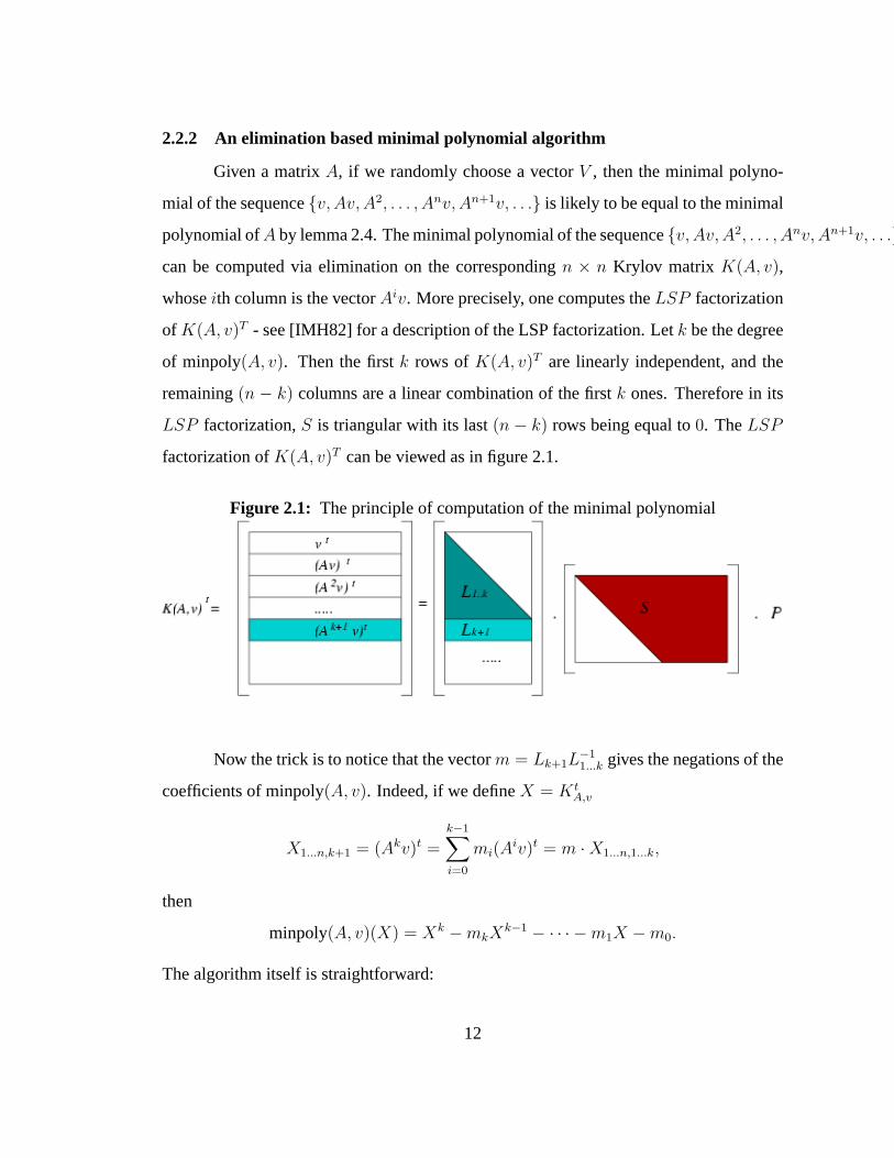
factorization ofK(A, v)T can be viewed as in figure 2.1.

Figure 2.1: The principle of computation of the minimal polynomial

Now the trick is to notice that the vectorm = Lk+1L−11...k gives the negations of the

coefficients of minpoly(A, v). Indeed, if we defineX = KtA,v

X1...n,k+1 = (Akv)t =k−1∑i=0

mi(Aiv)t = m ·X1...n,1...k,

then

minpoly(A, v)(X) = Xk −mkXk−1 − · · · −m1X −m0.

The algorithm itself is straightforward:

12

ALGORITHM 2.7. Elimination-basedminpoly(A, v)

Input:

• A, ann× n matrix over a fieldF

• v ∈ Fn, a column vector.

Output:

• minpoly(A, v), the minimal polynomial of the sequencev, Av, A2, . . . , Anv, An+1v, . . .

Procedure:

1. K1...n,1 = v

2. for i = 1 to log2 n[ComputeK(A, v)]

K1...n,2i...2i+1−1 = A2i−1K1...n,1...2i−1

3. (L, S, P ) = LSP(Kt), k = rank(K)

4. m = Lk+1.L−11...k

5. return minpoly(A, v)(X) = Xk +∑k−1

i=0 miXi

The dominant operation in this algorithm is the computation of the Krylov matrix,

in log2 n matrix multiplications, i.e. in O(nω log n) algebraic operations. The LSP factor-

ization requires O(nω) operations and the triangular system resolution, O(n2). Thus the

complexity of this algorithm is O(nω log n). When using classical matrix multiplications

(assumingω = 3), it is preferable to compute the Krylov matrix byn successive matrix

vector products. Then the number of field operations is O(n3).

2.3 Characteristic polynomials over a finite field

DEFINITION 2.8. For ann × n matrix A over a fieldF, the characteristic polynomial

of A is the polynomialp(x) defined by

p(x) = det(xIn − A).

13

We use charpoly(A) to denote the characteristic polynomial of a matrixA. We

will present a blackbox method and two elimination based methods for characteristic

polynomial over a finite field below.

2.3.1 A blackbox method

We use charpoly(A) to denote the characteristic polynomial of a matrixA.

DEFINITION 2.9. Given a monic polynomialp(x) = xn + an−1xn−1 + · · ·+ a1x + a0

the companion matrix ofp(x), denotedCp(x), is defined to be then × n matrix with 1’s

down the the first sub-diagonal and minus the coefficients ofp(x) down the last column,

or alternatively, as the transpose of this matrix.

Cp(x) =

0 0 . . . . . . . . . −a0

1 0 . . . . . . . . . −a1

0 1 . . . . . . . . . −a2

0 0... −a3

......

. .....

0 0 . . . . . . 1 −an−1

.

For a monic polynomial ofp(x), the characteristic polynomial and the minimal

polynomial of the companion matrixCp(x) is equal top(x).

A matrix over a field can be decomposed to an equivalent diagonal block matrix,

whose diagonal entries are companion matrices.

DEFINITION 2.10. If M is ann× n matrix over a fieldF, there is an invertible matrix

P such thatP−1MP = F where

F = M1 ⊕M2 ⊕ · · · ⊕Mt

14

where theMs are the companion matrices of what are known as the invariant polynomi-

als of M . If Mi is the companion matrix of a polynomialfi(x), and the characteristic

polynomial of M isfi(x), then

p(x) = f1(x)f2(x) · · · ft(x).

Eachfi dividesfi+1, if one writes the companion matricesMi such that asi increases,

so does the number of rows/columns ofMi. The polynomialft then is the minimal

polynomial of M.

For these companion matrices in the Frobenius normal form ofA, their charac-

teristic polynomials are also invariant factors ofxIn − A over F[x]. And the minimal

polynomial is the largest invariant factor ofxIn − A. All the invariant factors can be

computed by binary search - see [Vil00] for details.

2.3.2 Two elimination based methods

In [KG85], Keller-Gehrig gives anO(nω log(n)) algorithm for characteristic poly-

nomial over a finite fieldF. It works as follows:

• Findeij , 1 ≤ j ≤ k, such thatFn is equal to the direct sum of all the Krylov Spaces

of A andeij . This involves a complicated step-form elimination routine designed

for this application.

• ConstructU = ei1 , Aei1 , . . . , Ak1ei1 , ei2 , Aei2 , . . . a basis ofFn.

• U−1AU is block upper triangular, and the diagonal blocks are companion matri-

ces. Then, characteristic polynomial ofA is equal to the product the characteristic

polynomial of these companion blocks.

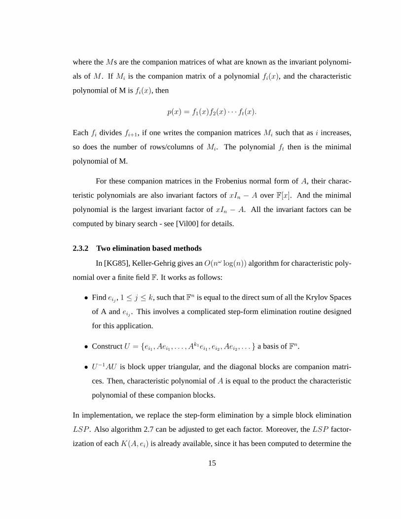
In implementation, we replace the step-form elimination by a simple block elimination

LSP . Also algorithm 2.7 can be adjusted to get each factor. Moreover, theLSP factor-

ization of eachK(A, ei) is already available, since it has been computed to determine the

15

linear dependencies withLSP . Therefore, the expensive part of minpoly(A, ei) can be

avoided. We can replace the complex step form elimination of Keller-Gehrig by the sim-

pler LSP factorization. Then, we have a straightforward method for finding the factors:

apply only the third step of the minpoly(A, v) algorithm, which is a triangular system

solve. The first two steps have already been computed. We have a straightforward dia-

gram for our implementation.

Figure 2.2: Diagram for Keller-Gehrig’s algorithm

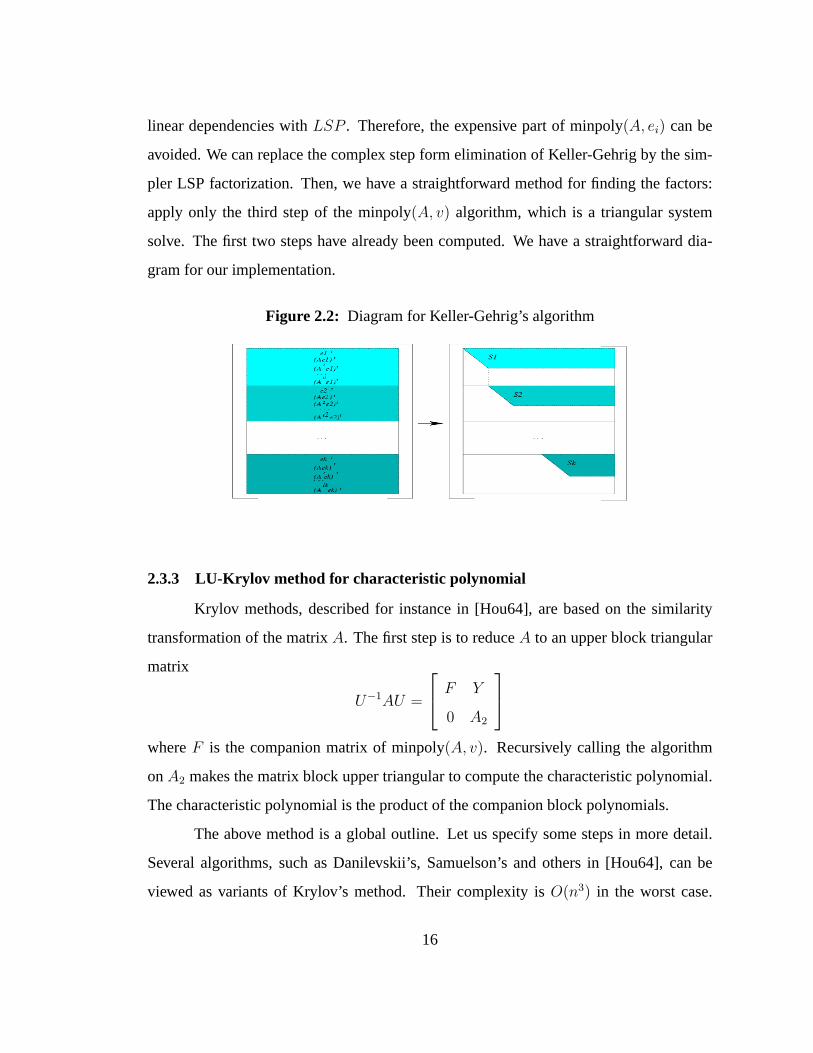
2.3.3 LU-Krylov method for characteristic polynomial

Krylov methods, described for instance in [Hou64], are based on the similarity

transformation of the matrixA. The first step is to reduceA to an upper block triangular

matrix

U−1AU =

F Y

0 A2

whereF is the companion matrix of minpoly(A, v). Recursively calling the algorithm

onA2 makes the matrix block upper triangular to compute the characteristic polynomial.

The characteristic polynomial is the product of the companion block polynomials.

The above method is a global outline. Let us specify some steps in more detail.

Several algorithms, such as Danilevskii’s, Samuelson’s and others in [Hou64], can be

viewed as variants of Krylov’s method. Their complexity isO(n3) in the worst case.

16

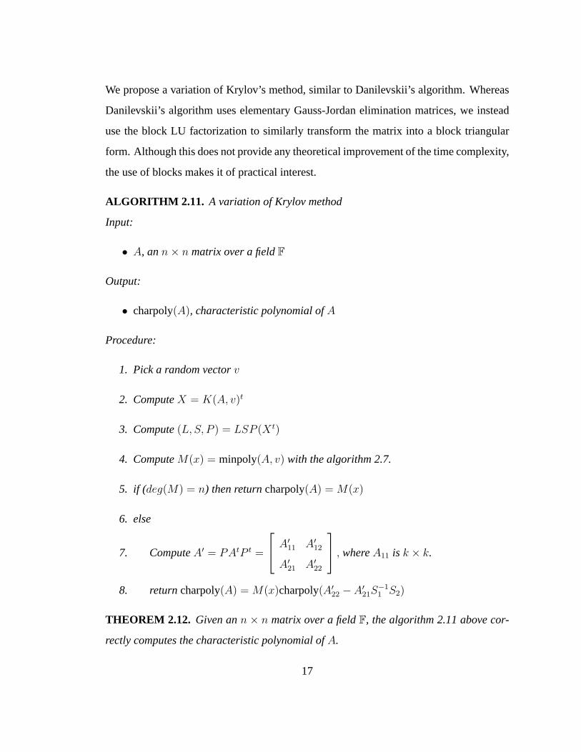
We propose a variation of Krylov’s method, similar to Danilevskii’s algorithm. Whereas

Danilevskii’s algorithm uses elementary Gauss-Jordan elimination matrices, we instead

use the block LU factorization to similarly transform the matrix into a block triangular

form. Although this does not provide any theoretical improvement of the time complexity,

the use of blocks makes it of practical interest.

ALGORITHM 2.11. A variation of Krylov method

Input:

• A, ann× n matrix over a fieldF

Output:

• charpoly(A), characteristic polynomial ofA

Procedure:

1. Pick a random vectorv

2. ComputeX = K(A, v)t

3. Compute(L, S, P ) = LSP (X t)

4. ComputeM(x) = minpoly(A, v) with the algorithm 2.7.

5. if (deg(M) = n) then returncharpoly(A) = M(x)

6. else

7. ComputeA′ = PAtP t =

A′11 A′

12

A′21 A′

22

, whereA11 is k × k.

8. returncharpoly(A) = M(x)charpoly(A′22 − A′

21S−11 S2)

THEOREM 2.12. Given ann × n matrix over a fieldF, the algorithm 2.11 above cor-

rectly computes the characteristic polynomial ofA.

17

Proof. The LSP factorization computes:

X =

L1

L2

[S1|S2]P

Let us deduce the invertible matrix

X =

L1 0

0 In−k

︸ ︷︷ ︸

L

S1 S2

0 In−k

︸ ︷︷ ︸

S

P =

X1..k[0 In−k

]P

Now X1..kAt = CtX1..k, whereC is the companion matrix associated to minpoly(A, v).

Therefore

XAtX−1

=

Ct 0[0 In−k

]PAtP tS

−1L−1

=

Ct 0[A′

21 A′22

]S−1

L−1

=

Ct 0

Y X2

whereX2 = A′

22−A′21S

−11 S2. So we know the algorithm 2.11 returns the correct answer.

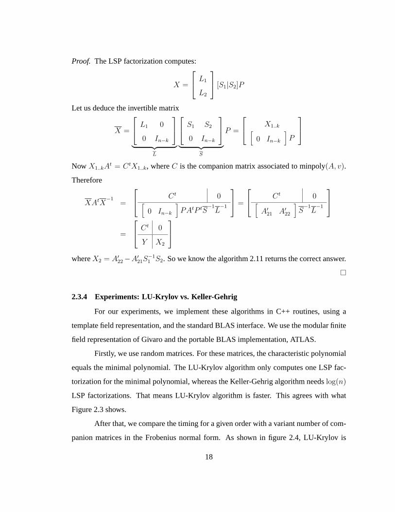
2.3.4 Experiments: LU-Krylov vs. Keller-Gehrig

For our experiments, we implement these algorithms in C++ routines, using a

template field representation, and the standard BLAS interface. We use the modular finite

field representation of Givaro and the portable BLAS implementation, ATLAS.

Firstly, we use random matrices. For these matrices, the characteristic polynomial

equals the minimal polynomial. The LU-Krylov algorithm only computes one LSP fac-

torization for the minimal polynomial, whereas the Keller-Gehrig algorithm needslog(n)

LSP factorizations. That means LU-Krylov algorithm is faster. This agrees with what

Figure 2.3 shows.

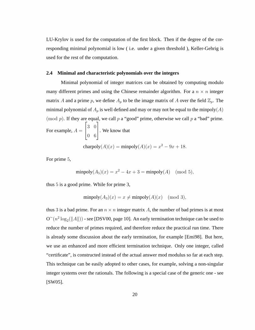
After that, we compare the timing for a given order with a variant number of com-

panion matrices in the Frobenius normal form. As shown in figure 2.4, LU-Krylov is

18

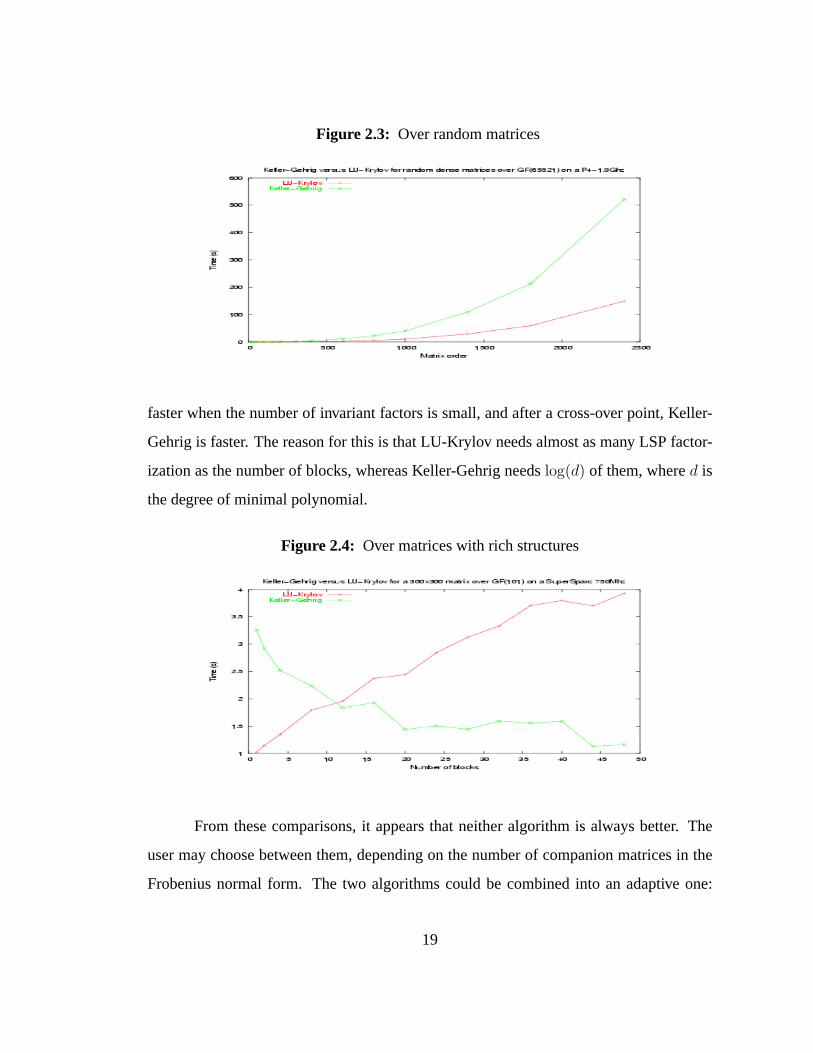
Figure 2.3: Over random matrices

faster when the number of invariant factors is small, and after a cross-over point, Keller-

Gehrig is faster. The reason for this is that LU-Krylov needs almost as many LSP factor-

ization as the number of blocks, whereas Keller-Gehrig needslog(d) of them, whered is

the degree of minimal polynomial.

Figure 2.4: Over matrices with rich structures

From these comparisons, it appears that neither algorithm is always better. The

user may choose between them, depending on the number of companion matrices in the

Frobenius normal form. The two algorithms could be combined into an adaptive one:

19

LU-Krylov is used for the computation of the first block. Then if the degree of the cor-

responding minimal polynomial is low ( i.e. under a given threshold ), Keller-Gehrig is

used for the rest of the computation.

2.4 Minimal and characteristic polynomials over the integers

Minimal polynomial of integer matrices can be obtained by computing modulo

many different primes and using the Chinese remainder algorithm. For an × n integer

matrixA and a primep, we defineAp to be the image matrix ofA over the fieldZp. The

minimal polynomial ofAp is well defined and may or may not be equal to the minpoly(A)

(mod p). If they are equal, we callp a “good” prime, otherwise we callp a “bad” prime.

For example,A =

3 0

0 6

. We know that

charpoly(A)(x) = minpoly(A)(x) = x2 − 9x + 18.

For prime5,

minpoly(A5)(x) = x2 − 4x + 3 = minpoly(A) (mod 5),

thus5 is a good prime. While for prime 3,

minpoly(A3)(x) = x 6= minpoly(A)(x) (mod 3),

thus3 is a bad prime. For ann× n integer matrixA, the number of bad primes is at most

O∼(n2 log2(‖A‖)) - see [DSV00, page 10]. An early termination technique can be used to

reduce the number of primes required, and therefore reduce the practical run time. There

is already some discussion about the early termination, for example [Emi98]. But here,

we use an enhanced and more efficient termination technique. Only one integer, called

“certificate”, is constructed instead of the actual answer mod modulus so far at each step.

This technique can be easily adopted to other cases, for example, solving a non-singular

integer systems over the rationals. The following is a special case of the generic one - see

[SW05].

20

ALGORITHM 2.13. Minimal polynomial with early termination

Input:

• A, ann× n integer matrix.

• P, a set of odd primes of sizeM, with minimal primeβ.

• Ω, the random sample size.

Output:

• v, coefficients of the minimal polynomial ofA.

Procedure:

1. Setl := 0, the length of the output vector.

2. Set listL := ∅, list of pair (good prime, minimal polynomial ofA mod it).

3. Choose a random vectorx of lengthn with entries independently and uniformly

chosen from[0, Ω− 1].

4. Uniformly choose a primep from P which has not been used before. Markp as

being used.

5. Computev = minpoly(A mod p)

If its degree is lower thanl , goto statement 3.

If its degree is larger thanl , setl to be this length, emptyL, append pair (p, vp) to

L, and goto statement 2.

If its degree is equal tol , append pair (p, vp) to L. Use the Chinese remainder

algorithm to construct a certificatec(i) wherei the size ofL, such thatc(i) = x · vq

(mod q), for each pair(q, vq) in L.

21

6. If c(i) 6= c(i−1), then goto statement 3. Otherwisec(i) = c(i−1), i.e., the termination

condition is met. Return the vectorv, which is constructed from pairs inL by the

Chinese remainder algorithm, such thatv = vq (mod q), for every pair (q, vq) in

L. This construction can be done by using a divide-and-conquer method.

REMARK.1. In order to capture negative numbers, we normalize the final numbera to

lie in [−(m− 1)/2, (m− 1)/2], wherem=∏

1≤i≤n pi.

2. The pre-selected primes idea in [Kal02] may be used here also. It works with

preselected prime stream so that one can pre-compute the constants which are indepen-

dent of the actual answer, for instance(p1 . . . pi)−1 mod pi+1 (The precomputed constant

will help if the Newton interpolation algorithm is applied to construct the final answer).

Such moduli are not random; additional post-check of the result at one additional ran-

dom moduli will guarantee the correctness of the final answer with very high probability.

Please see [Kal02] for more details.

THEOREM 2.14. Given ann × n integer matrix, if we choose the set of odd primes

to be odd primes of magnitude at mostnγ log n(log n + log2(‖A‖)) (γ is a real constant

bigger than2), then algorithm 2.13 above computes the minimal polynomial with error

probability at most2

Ω+ O(n2−γ).

It requiresO∼(n log2(‖A‖)) minimal polynomial computation over finite fields.

Note: For a typical problem, such as characteristic polynomial, or minimal poly-

nomial, it is easy to choose a reasonable set of primes and random sample size such that

the error probability is tiny. Runs are independent. If we repeat the algorithm, the error

probability is squared.

Proof. Let vectorα denote the correct answer andc denotex · α. We assume the early

termination condition is met at some numbern, i.e. c(n) is equal toc(n−1). If both |c| ≥

||α||∞ andc = c(n) are true, then the algorithm returns the correct answer. This is true

22

since the modulus, which is the product of the primes inL, is at least2||α||∞ under these

hypotheses. Therefore, there are only two sources of errors. One is the bad certificate.

The other is the premature termination.

The next statement explores the probability of a bad certificate. Ifx is a random

vector with entries independently and uniformly chosen from the integer set[0, Ω − 1],

then

Prob(|x · α|) < ||α||∞) ≤ 2

Ω.

This statement is true since there is at least one entry ofα, whose absolute value is equal

to ||α||∞. Without loss of generality, we assume|α0| = ||α||∞. Then for anyx1, . . . , xl−1,

there are at most two integersx0, such that|x · α| < ||α||∞. Therefore

Prob(|x · α|) < ||α||∞) ≤ 2

Ω.

Let us look at the probability of a premature termination. On the condition that

the early termination conditionc(n) = c(n−1) is met, the probability thatc 6= c(n) is at

O(n2−γ). This can be followed from the theorem [Kal02, Theorem 1.]. So the total error

probability is at most2

Ω+ O(n2−γ).

The number of the minimal polynomial calls over finite fields can be obtained

by estimating the maximal bit length for coefficients of minimal polynomialA - see e.g.

[KV03].

Combining Wiedemann’s algorithm and baby/giant step over the dense case, the

algorithm [Kal02, KV03] can compute the minimal polynomial with asymptotic improve-

ment from O∼(n4 log2(‖A‖)) to O∼(n3+1/3 log2(‖A‖)) with standard matrix multiplica-

tion.

23

In practice, it is often cheaper to compute minimal polynomial than characteristic

polynomial over the integers. In [KV03], Kaltofen and G. Villard point out that the char-

acteristic polynomial can be computed by using Hensel lifting on the minimal polynomial.

In [DPW05, section 4.4], the implementation detail has been presented.

2.5 An application

A key step in the computation of the unitary dual of a Lie group is to determine if

certain rational symmetric matrices are positive semi-definite. The computation of signa-

tures of certain matrices which are decided by root systems and facets(see e.g. [ASW05])

can help classify the unitary representations of Weyl groups. The most interesting case is

that ofE8, which is a Weyl group with order696, 729, 600. E8 has112 representations,

the largest of which has dimension7, 168. Though results onE8 are known, our succes-

sive computation will encourage to calculate the unitary dual of more general cases such

as Hecke algebras, real andp-adic Lie groups.

The minimal polynomial can be used to determine positive (negative) definiteness

and positive (negative) semi-definiteness. By Descartes’ rule, the characteristic polyno-

mial can be used to determine the signature which is the difference of positive eigenvalues

and negative ones. These special rational matrices from Lie groups representation can be

scaled to integer matrices by multiplying by the lcm of the denominators of all entries.

For these specially constructed matrices from Lie group representation, the lcm of the de-

nominators of all entries is just a little larger than each individual one. This transformation

keeps the signature.

On a challenge facet1/40(0, 1, 2, 3, 4, 5, 6, 23) cases, all constructed rational ma-

trices are non-singular and we verified that all these rational matrices of dimension up to a

few thousand are positive definite. On another special facet(0, 1/6, 1/6, 1/4, 1/3, 5/12, 7/12, 23/12),

all constructed rational matrices have low ranks and we verified all matrices (largest di-

mension7, 168) are positive semi-definite. Our success experiments shows the computa-

tion for classifying the representation of Lie groups is feasible.

24

Chapter 3

COMPUTATION OF THE RANK OF A MATRIX

3.1 Introduction

Determining the rank of a matrix is a classical problem. The rank of an integer

matrix can be probabilistically determined by computation modulo a random prime. The

rank of an integer matrix can also be certified by using its trace - see [SSV04] for details.

It can be made to be deterministic if the rank is determined by computation modulo a

sufficient number of distinct primes.

For a dense matrix over a finite field, its rank can be found by using Gaussian

elimination. Moreover, pivoting in Gaussian elimination is not as important in exact

computation as it is in numerical Gaussian elimination. In the numeric linear method,

the answer is approximate due to floating point rounding errors, and a pivoting strategy

is used to improve the accuracy of the answer and make the algorithm backward stable.

But in symbolic computation, only exact field operations are used, and the algorithm

always gives the correct answer. A block implementation such as [DGP04] speeds up the

practical run time of Gaussian elimination.

However, there are choices of algorithms for large sparse matrices. For a sparse

matrix over a finite field, its rank can be computed by either Krylov space methods such

as Wiedemann’s method [Wie86, KS91], and block Wiedemann’s algorithm [Cop95,

Kal95], or sparse elimination such as SuperLU. Each algorithm is favorable to certain

cases. In practice, it is hard to make the choice of algorithms for a given sparse matrix.

We contribute an adaptive (introspective) algorithm to solve this puzzle. This adaptive

25

method is obtained by carefully studying each algorithm and comparing these two dis-

tinct methods. It works by starting with an elimination and switching to a Krylov space

method if a quick rate of fill-in is detected. We have studied two typical methods. One

method is GSLU (Generic SuperLU) [DSW03], an adaptation of the SuperLU method

[Sup03], and a fundamentally Gaussian elimination method with special ordering strate-

gies. The second method, called here BB for “black box”, is a variant of the Krylov

space-based Wiedemann’s algorithm [Wie86]. Our experiment shows that our adaptive

method is feasible and very efficient. The adaptive idea may be easily adopted to other

problems such as computing determinants and solving linear systems. The observations

made here apply quite directly to those problems.

A portion of the work in this chapter were presented at SIAMLA 2003 [DSW03]

and ACA2003[LSW03].

3.2 Wiedemann’s algorithm for rank

DEFINITION 3.1. The rank of a matrix over a field is the dimension of the range of the

matrix. This corresponds to the number of linearly independent rows or columns of the

matrix.

Algorithm 2.6 can be used to compute the minimal polynomial of a matrix over

finite fields. With preconditioning as in [EK97, KS91, CEK+02], it likely has no nilpo-

tent blocks of size greater than1 in its Jordan canonical form (i.e.x2 doesn’t divide its

minimal polynomial) and its characteristic polynomial will be equal to the shifted min-

imal polynomial with high probability. We define theshifted minimal polynomialto be

the polynomial which is the product of the minimal polynomial and a power ofx and

has degree of the matrix’s order. In the case that a matrix has no nilpotent blocks of size

greater than1 in its Jordan canonical form, the rank can be determined from the charac-

teristic polynomial and is equal to the degree of its characteristic polynomial minus the

26

multiplicity of its zero roots. The next theorem is from [CEK+02, Theorem 4.7] about

diagonal preconditioning for the symmetric case.

THEOREM 3.2. LetA be a symmetricn×n matrix over a fieldF whose characteristic is

0 or greater thann and letS be a finite subset ofF\0. If d1, . . . , dn are chosen uniformly

and independently fromS and D = diag(d1, . . . , dn), then the matricesA and DAD

have the same rank, the minimal polynomial ofDAD is square free, and the characteristic

polynomial is the production of the minimal polynomial and a power ofx, with probability

at least1− 4n2/#S. This probability increases to1− 2n2/#S if the squares of elements

of S are distinct.

Note that if the minimal polynomial is square free, then the matrix has no nilpotent

blocks of size greater than1 in its Jordan canonical form. For the non-symmetric case, an

additional random diagonalD may be used. We have the following lemma:

LEMMA 3.3. LetA be a non-symmetricn×n matrix over a fieldF whose characteristic

is 0 or greater thann and letS be a finite subset ofF. If d1, . . . , dn are chosen uniformly

and independently fromS and D = diag(d1, . . . , dn), then the matricesA and AT DA

has the same rank with probability at least1− n/#S.

Proof. This is a simple case in [EK97, lemma 6.1]. Note that the matrixAT DA can be

viewed as a polynomial matrix overF[d1, . . . , dn] and has the same rank asA. So there

is a non-singular sub-matrix ofAT DA with dimension ofA’s rank. So the determinant

of this sub-matrix is a multi-variable polynomial overF[d1, . . . , dn] with total degree at

mostn. By the Schwartz-Zippel lemma [Sch80], the probability that this determinant is

equal to0 is at mostn/#S.

Wiedemann’s algorithm for the rank using diagonal preconditioning is straightfor-

ward.

ALGORITHM 3.4. Wiedemann’s algorithm for rank

Input:

27

• A, a n× n matrix over a finite fieldF

Output:

• The rank ofA

Procedure:

1. Choosen × n diagonal matricesD1 andD2 with diagonal entries uniformly and

independently fromF\0.

2. Compute the minimal polynomial ofD2AT D1AD2

3. If the constant coefficient of the minimal polynomial is non-zero, return its degree.

Otherwise, return its degree -1.

Note thatD2AT D1AD2 can be viewed as a composition of the blackbox matrices

D2, AT , D1, A,D2 and can be used as a blackbox. That is,D2A

T D1AD2 doesn’t need to

be computed explicitly and its matrix-by-vector product can be computed via a sequence

of matrix-by-vector products ofD2, A,D1. Other preconditioning like Toeplitz matrices,

sparse matrices may be used also - see [EK97, KS91, CEK+02]

3.3 GSLU: a sparse elimination

GSLU (Generic SuperLU) is adapted to LinBox library from SuperLU version 2.0

[Sup03] and can be used with arbitrary fields including finite field representations. Basic

GSLU is an elimination method, and uses pre-ordering to keep sparsity ofL andU during

elimination. There are five possible ordering choices (natural ordering, multiple minimum

degree applied to structureAT A, multiple minimum degree applied to structureAT + A,

column approximation minimum degree, and supplied by user as input) for pre-ordering

the columns of a matrixA. After that, a column-based Gaussian elimination is used. It

works like the incremental rank method, first performingLUP in the firstk columns,

adding the(k + 1)th column and updating L, U and P. We call time updating L, U and P

the(k + 1)th step time.

28

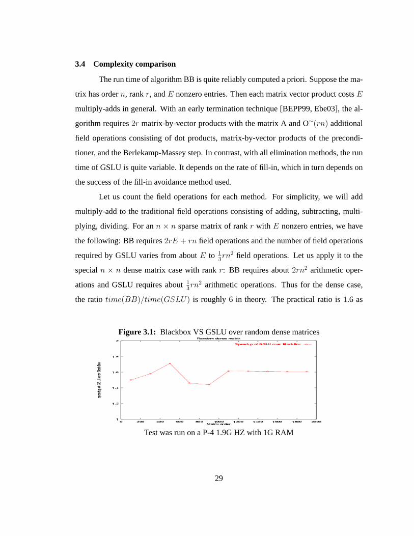
3.4 Complexity comparison

The run time of algorithm BB is quite reliably computed a priori. Suppose the ma-

trix has ordern, rankr, andE nonzero entries. Then each matrix vector product costsE

multiply-adds in general. With an early termination technique [BEPP99, Ebe03], the al-

gorithm requires2r matrix-by-vector products with the matrix A and O∼(rn) additional

field operations consisting of dot products, matrix-by-vector products of the precondi-

tioner, and the Berlekamp-Massey step. In contrast, with all elimination methods, the run

time of GSLU is quite variable. It depends on the rate of fill-in, which in turn depends on

the success of the fill-in avoidance method used.

Let us count the field operations for each method. For simplicity, we will add

multiply-add to the traditional field operations consisting of adding, subtracting, multi-

plying, dividing. For ann × n sparse matrix of rankr with E nonzero entries, we have

the following: BB requires2rE + rn field operations and the number of field operations

required by GSLU varies from aboutE to 13rn2 field operations. Let us apply it to the

specialn × n dense matrix case with rankr: BB requires about2rn2 arithmetic oper-

ations and GSLU requires about13rn2 arithmetic operations. Thus for the dense case,

the ratiotime(BB)/time(GSLU) is roughly 6 in theory. The practical ratio is 1.6 as

Figure 3.1: Blackbox VS GSLU over random dense matrices

Test was run on a P-4 1.9G HZ with 1G RAM

29

demonstrated in figure 3.1, due to our special optimal implementation for matrix-by-

vector product.

For the general sparse case, it is very difficult to predict which method will run

faster. Generally speaking, BB is superior for very large matrices, in particular when

fill-in causes the matrix storage to exceed machine main memory and even exceed the

available virtual memory. In practice, fill-in is hard to detect. Evidently, there are some

small dimension matrices (less then200× 200) for which BB is faster than GSLU, while

there are some very huge dimension sparse matrices, close to100, 000 × 100, 000, for

which GSLU is much faster than BB.

3.5 An adaptive algorithm

Due to the uncertain run time of algorithms for computing the rank of a sparse ma-

trix, it is desirable to have an algorithm that can intelligently choose among various avail-

able algorithms for computing the rank and the given matrix. We call such an algorithm

an adaptive algorithm. For computing the rank of a sparse matrix, our adaptive algorithm

starts with a sparse elimination algorithm, but may switch to a blackbox algorithm under

certain appropriate conditions. Let us explore more properties about the sparse elimina-

tion algorithm, GSLU. The GSLU algorithm is a “left looking” elimination, which has

the consequence that the cost of elimination steps tends to be an increasing function of

step number. After testing on many examples, we observe that GSLU will increase the

time for each step dramatically at a very early stage, then step time will increase very

slowly and never decrease. This gives us a chance to recognize rapid growth of step cost

and switch to the BB method at a relatively early stage. At each step we can estimate the

remaining cost by assuming the same cost for all future steps (the rectangular region in

the figure). If it exceeds BB cost, we switch.

30

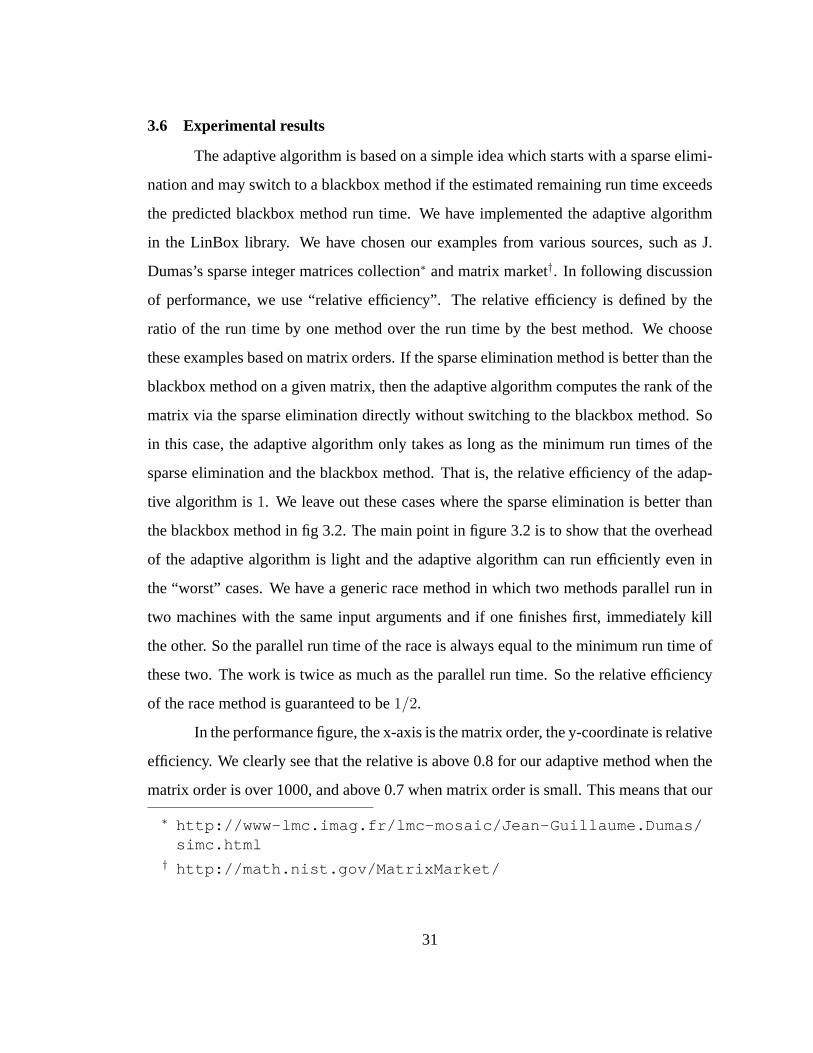
3.6 Experimental results

The adaptive algorithm is based on a simple idea which starts with a sparse elimi-

nation and may switch to a blackbox method if the estimated remaining run time exceeds

the predicted blackbox method run time. We have implemented the adaptive algorithm

in the LinBox library. We have chosen our examples from various sources, such as J.

Dumas’s sparse integer matrices collection∗ and matrix market†. In following discussion

of performance, we use “relative efficiency”. The relative efficiency is defined by the

ratio of the run time by one method over the run time by the best method. We choose

these examples based on matrix orders. If the sparse elimination method is better than the

blackbox method on a given matrix, then the adaptive algorithm computes the rank of the

matrix via the sparse elimination directly without switching to the blackbox method. So

in this case, the adaptive algorithm only takes as long as the minimum run times of the

sparse elimination and the blackbox method. That is, the relative efficiency of the adap-

tive algorithm is1. We leave out these cases where the sparse elimination is better than

the blackbox method in fig 3.2. The main point in figure 3.2 is to show that the overhead

of the adaptive algorithm is light and the adaptive algorithm can run efficiently even in

the “worst” cases. We have a generic race method in which two methods parallel run in

two machines with the same input arguments and if one finishes first, immediately kill

the other. So the parallel run time of the race is always equal to the minimum run time of

these two. The work is twice as much as the parallel run time. So the relative efficiency

of the race method is guaranteed to be1/2.

In the performance figure, the x-axis is the matrix order, the y-coordinate is relative

efficiency. We clearly see that the relative is above 0.8 for our adaptive method when the

matrix order is over 1000, and above 0.7 when matrix order is small. This means that our

∗ http://www-lmc.imag.fr/lmc-mosaic/Jean-Guillaume.Dumas/simc.html

† http://math.nist.gov/MatrixMarket/

31

Figure 3.2: Experimental result of adaptive algorithm

adaptive algorithm of elimination and Blackbox methods is advisable and very effective

in practice.

32

Chapter 4

COMPUTATION OF EXACT RATIONAL SOLUTIONS FOR

LINEAR SYSTEMS

4.1 Introduction

Finding the rational solution of a non-singular integer linear system is a classic

problem. In contrast to numerical linear methods, the solution is computed symbolically

(exactly) without any error. Rational solving can be applied to solve the Smith form

problem, Diophantine equations, etc. By Cramer’s rule, there is a unique solution to

a non-singular integer linear system. The modular method is a good way to find the

exact solution. The solution can be found either by computation modulo many distinct

primes and the Chinese remainder algorithm or byp-adic lifting [Dix82, MC79], a special

case of Hensel lifting [vzGG99, section 15.4]. The latter is better, since the asymptotic

complexity ofp-adic lifting is cheaper by a factor of O∼(n) than the first one. It is not

a good idea to find the rational solution of a non-singular integer linear system by using

Gaussian elimination over the rationals. For ann× n non-singular integer matrixA, and

a column integer vectorb, the solution ofAx = b is a column vector with rational entries

whose numerators and denominators have O∼(n(log2(‖A‖) + ||b||∞)) bits. Thus the cost

using Gaussian elimination over the rationals will be O∼(n4(log2(‖A‖) + ||b||∞)). This

method costs by an O∼(n) factor more expensive thanp-adic lifting and is not memory

efficient.

We contribute a new algorithm which works in well-conditioned cases with the

same asymptotic complexity as thep-adic lifting and aborts quickly in ill-conditioned

33

cases. Success of this algorithm on a linear equation requires the linear system to be suf-

ficiently well-conditioned for the numerical linear algebra method being used to compute

a solution with sufficient accuracy. This approach will lead to high performance in prac-

tice. Another contribution is an adaptive algorithm for computing the exact solution of a

non-singular linear system. The idea is to start with our new algorithm, and if it aborts,

switch top-adic lifting.

4.2 p-adic lifting for exact solutions

Working with a primep, developing solutions modpk (i.e. in p-adic arithmetic),

and finally reconstructing the rational solution can be used to find the exact solutions of

linear equations. The rational reconstruction can be done using the Euclidean algorithm

for the gcd of two integers - see [vzGG99, section 5.7]. The following is the outline of

this method:

ALGORITHM 4.1. p-adic lifting for exact solutions

Input:

• A, ann× n non-singular integer matrix

• b ∈ Zn, a column vector

• p, a prime such thatp 6 |det(A)

Output:

• x ∈ Qn, the rational solution ofAx = b.

Procedure:

1. Computeδ = βnnn/2, which bounds absolute values of numerators and denomina-

tors of solution toAx = b. Whereβ is a bound on the absolute values of entries of

A andb.

34

2. ComputeC such thatCA = In (mod p)

3. Setb0 = b

4. Computex0 = Cb0 (mod p)

5. For i = 0 to 2dlog δ/ log pe do

• Computebi+1 = p−1(bi − Axi)

• Computexi+1 = Cbi+1 (mod p)

6. Rationally reconstructx

THEOREM 4.2. The algorithm 4.1 above correctly computes the rational solution and

requiresO∼(n3 log2(‖A‖)) bit operations.

Proof. See [Dix82] for details.

Algorithm 4.1 can be modified to work with sparse matrices by replacing the

method of solving the linear system modulop by Wiedemann’s method (see algorithm

2.6). In step 5, each solution will be involved with degree(minpoly(A)) matrix-by-vector

products. It requires totallyn2 log2(‖A‖) matrix-by-vector products in the worst case.

Thus the algorithm will be no more of efficient time, but it can save space.

4.3 Using numerical methods

Both symbolic methods and numerical methods can be used to solve linear sys-

tems. But the tow methods use different techniques and have been developed indepen-

dently. Symbolic methods for solving linear systems are based on modular methods via

solving the linear system modulo a large integer and finally reconstructing the rational

solution. Eitherp-adic lifting [Dix82, MC79] or computation modulo many different

primes and using the Chinese remainder algorithm are the widely used methods to com-

pute solutions of linear systems modulo a large integer. Numerical methods use either

35

direct methods like Gaussian Elimination (with or without pivoting),QR factorization,

or iterative methods such as Jacobi’s method, Lanczos’ method, or the GMRES method

- see [Dem97, Saa03, TB97] for details. Symbolic methods for solving linear systems

can deliver the correct answer without any error, though they are usually more expensive

in computation time than numerical methods. But numerical linear algebra methods for

solving linear systems are subject to the limitation of floating point precision and iterative

methods are subject to additional convergence problems.

In this section, we describe a new algorithm to exactly solve well-conditioned in-

teger linear systems using numerical methods. A portion of this work has been submitted

to the journal of symbolic computation [Wan04]. A secondary benefit is that it aborts

quickly in ill-conditioned cases. Success of this algorithm requires the system to be suf-

ficiently well-conditioned for the numeric linear algebra method being used to compute

a solution with sufficient accuracy. Though this algorithm has the same asymptotic cost

asp-adic lifting, it yields practical efficiency. The practical efficiency results from the

following two things. First, over the past few decades, hardware floating point operations

have been sped up dramatically, from a few hundred FLOPS in 1940s to a few GFLOPS

now, even in PCs. Second, many high performance numerical linear algebra packages

have been developed using fast BLAS implementation for dense systems.

The motivation for this algorithm is the high performance of numerical linear al-

gebra packages and the simple fact below:

FACT 4.3. If two rational numbersr1 = ab, r2 = c

dare given withgcd(a, b) = 1,

gcd(c, d) = 1, andr1 6= r2, then|r1 − r2| ≥ 1bd

.

That is, rational numbers with a bounded denominators are discrete, though it is

well known that all rational numbers are dense in the real line. Because of this simple

fact, if a solution with very high accuracy can be computed, then the rational solution can

be reconstructed.

36

In general, numerical methods are inexact when carried out on a computer: an-

swers are accurate up to at most machine precision (or software floating point precision).

In order to achieve more accuracy than machine precision, our idea is straightforward:

approximation, amplification, and adjustment. We first find an approximate solution with

a numerical method, then amplify the approximate solution by a chosen suitable scalar,

adjust the amplified approximate solution and corresponding residual so that they can be

stored exactly as integers of small magnitude. Then repeat these steps until a desired

accuracy is achieved. The approximating, amplifying, and adjusting idea enables us to

compute the solution with arbitrarily high accuracy without any high precision software

floating point arithmetic involved in the whole procedure or big integer arithmetic in-

volved except at the final rational reconstruction step. Detail will be discussed in section

4.5.

The next section is a classic result about the rational reconstruction. Continued

fractions which give the best rational approximations of real numbers enable us to recon-

struct a rational number with certain constraints from a real number. In the following

section, we describe a way to achieve arbitrary accuracy using numerical linear methods,

on the condition that inputs are integers and matrices are well-conditioned. Finally the

potential usage of our new algorithms for sparse linear systems is demonstrated with a

challenging problem.

4.4 Continued fractions

The best approximation with a bounded denominator of a real number is a segment

of its continued fraction. Just as a quick reminder, a brief description of the continued

fraction is given. For a real numberr, a simple continued fraction is an expression in the

form

r = a0 +1

a1 + 1a2+ 1

a3+···

,

37

where allai are integers. From now on, we assume that ifr ≥ 0, thena0 ≥ 0, all ai > 0

for i ≥ 1, and if r < 0, thena0 ≤ 0, all ai < 0 for i ≥ 1. A more convenient notation

is r = [a0; a1, a2, · · · ]. Intuitively, we can apply the extended Euclidean algorithm to

compute the simple continued fraction of a rational number.

For example, letr = 37961387

. We can computegcd(3796, 1387) using Euclid’s al-

gorithm, 3796 = 1387 · 2 + 1022; 1387 = 1022 · 1 + 365; 1022 = 365 · 2 + 292;

365 = 292 · 1 + 73; 292 = 73 · 4. We re-write these equations,3796/1387 = 2 +

1022/1387 = 2 + 1/(1387/1022) = 2 + 1/(1 + 365/1022) = 2 + 1/(1 + 1/(1022/365))

= 2 + 1/(1 + 1/(2 + 292/365) · · · = 2 + 1/(1 + 1/(2 + 1/(1 + 4))) = [2; 1, 2, 1, 4].

For a simple continued fraction forr (either finite or infinite) one defines a family

of finite segmentssk = [a0; a1, a2, ..., ak], eachsk being a rational number:sk = pk/qk

with qk > 0 andgcd(pk, qk) = 1. Below we list a few properties of the simple continued

fraction inr ≥ 0 cases. There are similar properties inr < 0 cases. Further detail about

these properties can be found on the internet, for example

http://www.cut-the-knot.org/do_you_know/fraction.shtml and

http://mathworld.wolfram.com/ContinuedFraction.html .

1. Every rational number can be associated with a finite continued fraction. Irrational

numbers can also be uniquely associated with simple continued fractions. If we

exclude the finite fractions with the last quotient equal to1, then the correspondence

between rational numbers and finite continued fractions becomes one to one.

2. For allk ≥ 2, pk = akpk−1 + pk−2, qk = akqk−1 + qk−2.

3. qkpk−1 − pkqk−1 = (−1)k. And sk − sk−1 = (−1)k−1/(qkqk−1).

4. s0 < s2 < s4 < s6 < · · · < r < · · · < s7 < s5 < s3 < s1.

Based on the nice properties about continued fraction above, now we can prove:

38

THEOREM 4.4. Given r, B > 0 there is at most one rational solutionab

such that

|ab− r| < 1

2Bb, 0 < b ≤ B, andgcd(a, b) = 1. Moreover, if there is one rational solution

ab, then for somek, a

b= pk

qk, where(pk, qk) is a segment of the simple continued fraction

of r, such that eitherpk/qk = r or qk ≤ B < qk+1. Moreover, ifr = nd, then there is an

algorithm to compute(pk, qk), which requiresO(M(l) log l) bit operations, , wherel is

the maximum bit length ofn andd.

Note: if B = 1, then there is either no solution orab

=nearest integer to r

1.

Proof. First we prove there is at most one solution. By way of contradiction, if there are

two different rational solutionsa1

b1and a2

b2with

0 < b1, b2 ≤ B, gcd(a1, b1) = gcd(a2, b2) = 1,a1

b1

6= a2

b2

.

Then

|a1

b1

− a2

b2

| ≤ |a1

b1

− r|+ |a2

b2

− r| < 1

2Bb1

+1

2Bb2

<1

b1b2

.

This is a contradiction to|a1

b1− a2

b2| ≥ 1

b1b2from Fact 4.3. So there is at most one solution.

For the given real numberr, we assumek is the unique integer number, such that

eitherpk/qk = r or qk ≤ B < qk+1.

If ab

is a solution with0 < b ≤ B, andgcd(a, b) = 1. Then we need to proveab

= pk

qk. By

way of contradiction, supposeab

is a solution andab6= pk

qk. If pk/qk = r, thenpk

qkis another

rational solution, and we have a contradiction. Ifqk ≤ B < qk+1, then by property 3,

|pk

qk

− pk+1

qk+1

| = 1

qkqk+1

.

And by fact 1 and the assumption,qk ≤ B < qk+1,

|ab− pk

qk

| ≥ 1

bqk

>1

qkqk+1

.

So ab

doesn’t lie betweenpk

qkand pk+1

qk+1. On the other hand,r must lie betweenpk

qkand pk+1

qk+1

by property 4. Thus

|ab− r| ≥ min(|a

b− pk

qk

|, |ab− pk+1

qk+1

|) ≥ 1

bqk+1

.

39

And by the assumptionab

is a solution,|ab− r| < 1

2Bb. Therefore 1

2Bb> 1

bqk+1. Thus

qk+1 > 2B. So,

|pk

qk

− r| ≤ |pk

qk

− pk+1

qk+1

| = 1

qkqk+1

<1

2qkB.

Thereforepk

qkis another solution. This is a contradiction to what we have proven that there

is at most one solution.

If r = nd, the (pk, qk) can be computed by the half gcd algorithm - please see

e.g.[vzGG99, Corollary 11.10]. It needs O(M(l) log l) bit operations.

4.5 Exact solutions of integer linear systems

In this section, we present a new way to exactly compute the solution of a non-

singular linear system with integer coefficients, repeatedly using a numerical linear alge-

bra method. As is common in numerical analysis, we will use the infinity-norm in the

performance analysis. Specifically, for an × m matrix A = (aij), we define||A||∞ =

max1≤i≤n

∑1≤j≤m |aij|, and for a vectorb of lengthn, we define||b||∞ = max1≤j≤n|bj|.

It is well known that numerical linear algebra methods are inexact and the accuracy

of the solutions is limited to machine precision (or the software floating point precision),

when carried out on a computer. Iterative refinement methods (see e.g. [FM67, Dem97,

GZ02]) can be used to refine the solution. The refinement, [GZ02] in which a portion,

not all, of high precision floating point arithmetics is replaced by lower precision floating

point arithmetics, is very efficient in computing a solution with a pre-set high precision.

It works this way: for inputA, b, and a pre-set precision, initially solveAx = b in

the hardware floating point precision (lower than the pre-set high precision), repeat the

following steps enough times to refine the answer until the desired accuracy is achieved:

r = b − Ax in a higher precision proportional to the step count, solveA ·∆x = r in the

hardware floating point precision, updatex = x + ∆x in a higher precision proportional

to the step count. These refinement methods help compute solutions with a reasonable

high accuracy at affordable practical run time cost and worst case complexity cost.

40

In symbolic linear algebra, however, the high accuracy of solutions required in

order to reconstruct the exact answer makes these iterative methods impractical. All the

refinement methods above require floating point operations in high precision. And the

cost of one software floating point operation increases rapidly with respect to the preci-

sion, which has been illustrated in [GZ02, Figure 1]. Also, these refinement methods lead

to more expensive complexity for the worst case than thep-adic lifting method. Thus for

symbolic computation, we need a better refinement method. Our approximating, ampli-

fying and adjusting idea works as follows: For input integer matrixA and integer vector

b. First initialize the solutionx = 1d· n with d = 1 and vectorn = 0 and initialize the

residualr = b. Then repeat the following steps until we achieve a desired accuracy: find

an approximate solutionA · ∆x = r in the hardware floating point arithmetic, choose a

suitable scalarα, amplify and adjust the∆x with rationals 1∆d· ∆n by setting∆d = α,

∆n = (≈ α · ∆x1, . . . ,≈ α · ∆xn), update answer:n = α · n + ∆n andd = ∆d · d,

update residualr = α · r − A ·∆n. In each refinement iteration, the components of the

amplified and adjusted residual are integers of magnitude at most||b||∞ + ||A||∞. Our

method can be used to achieve any arbitrary high accuracy of the answers without high

precision software floating point arithmetic involved in the whole procedure or big integer

arithmetic involved except the final rational reconstruction step. After sufficient accuracy

is achieved, the final rational solution can be reconstructed.

4.5.1 An exact rational solver for dense integer linear systems

We apply our main idea described above to dense linear systems in detail.

ALGORITHM 4.5. An exact rational solver for dense case

Input:

• A, a non-singularm×m integer matrix.

• b, a right hand side integer vector.

41

Output:

• x ∈ Qm, the rational solution ofAx = b. Or it aborts with message ”insufficient

numerical accuracy”.

Procedure:

1. Compute aLUP factorization ofA in floating point arithmetic using a backward

stable numeric method.[Other factorizations may be used here too.]

2. Set integerd(0) := 1. [The common denominator of the answer.]

3. Set integer vectorr(0) := b. [The residual.]

4. Set integeri := 0. [Step counter]

5. Compute integerB, the Hadamard bound ofA, which bounds the determinant and

all (m− 1)× (m− 1) minors ofA.

6. repeat the following steps untild(i) > 2m ·B2(2−i||b||∞ + ||A||∞).

6.1 i := i + 1.

6.2 Computex(i) = A−1r(i−1) in floating point arithmetic using theLUP factor-

ization from step 1.[An approximate solutionAx = r(i−1).]

6.3 Compute the integer scalar,α(i) := min(230, 2blog2(

||r(i−1)||∞||r(i−1)−Ax(i)||∞

)−1cin float-

ing point arithmetic;[For the purpose of high performance,α should be cho-

sen to be a power of 2, because in this case, operations of integers multiplying

theα can be replaced by more efficient operations of shifting bits. For small

size systems, the approximate answer might equal the exact answer. The con-

stant makes the algorithm work in the small size cases. Also, 30 is chosen

so that the amplified and adjusted solution and residual can be exactly repre-

sented by hardware double floating point numbers.]

42

6.4 Ifα(i) < 2, abort with error message ”insufficient numerical accuracy”.[This

situation happens only ifA is ill-conditioned.]

6.5 Exactly compute integer vectorx(i) := ([α(i) · x(i)1 ], . . . , [α(i) · x(i)

m ])s, where[]

means to round to the nearest integer.

6.6 Exactly compute integerd(i) := d(i−1) · α(i).

6.7 Exactly compute integer vectorr(i) := α(i) · r(i−1) − Ax(i). [Amplify the

residual by a scalar.]

7. Setk := i

8. Compute integer vectorn(k) =∑

1≤i≤kd(k)

d(i) · x(i), noting d(k)

d(i) =∏

i<j≤k α(j).

9. Reconstruct rational solutionx from 1d(k) ·n(k) using Theorem 4.4 with denominators

bounded byB.

10. Returnx.

Note:

1. This algorithm requires the input matrix to be sufficiently well-conditioned for the

numerical solver being used to work successfully. If the matrix is ill-conditioned, it

is a nice and important property of our algorithm that we quickly detect the failure

rather than continuing a nonsensical successive refinement.

2. In solving a linear system, estimating the residual usually is easier than estimating

the error. Obviously, the infinity norm of the error is bounded by the product of the

infinity norms of the inverse of the input matrix and the residual. In theith iterator,

r(i), the infinity norm of the residual is approximately1α(i) times the previous one,

by the choice ofα(i). Thus the infinity norm of the residual is approximately1d(i) .

Soe(i), the infinity norm of the error is at most approximately||A−1||∞d(i) . By Cramer’s

rule, we know||A−1||∞ ≤mB. Thus roughly speaking,ei ≤ mBd(i) . Careful analysis

43

shows thatri ≤||b||∞

2i +||A||∞d(i) . Thus if the loop ends without abortion, the error will

be at most 12Bd(k) , and then by theorem 4.4, the correct solution can be constructed

from the approximate solutionn(k)

d(k) .

THEOREM 4.6. If theα(i) in step 6.3 is not over computed in each iteration, that is,α(i)

is no larger than the actual value of ||r(i−1)||∞2||r(i−1)−Ax(i)||∞

due to floating point approximation,

then the algorithm above will either abort or terminate with the correct rational solution

in theith iteration,

||r(i)||∞ = ||d(i)(b− A1

d(i)· n(i))||∞ ≤ 2−i||b||∞ + ||A||∞.

Proof. On the input ofA andb, if the algorithm aborts, the statement is true. Otherwise,

we need to show the algorithm terminates with the correct rational answer. First we show

the algorithm will terminate. Since it doesn’t abort, eachα(i) is no less than2. Let us

estimated(i),

d(i) =∏

1≤j≤i

α(j) ≥∏

1≤j≤i

2 = 2i.

Thus the loop inside the algorithm runs through finitely many iterations. The algorithm

will terminate.

Now we prove the correctness. Letn(i) =∑

1≤j≤id(i)

d(j) · x(j), the numerator of the

accumulated solution after the firsti iterations. We need to estimatee(i) = || 1d(i) · n(i) −

A−1b||∞, the norm of the absolute error of the solution in each iteration. By induction,

we can prove that

r(i) = d(i)(b− A1

d(i)· n(i)). So

e(i) = || 1

d(i)· n(i) − A−1b||∞ =

1

d(i)||A−1r(i)||∞.

44

Now we need to estimate||r(i)||∞. In each iteration, by the hypotheses of the theorem,

we have||Ax(i)− r(i−1)||∞ ≤ 12α(i) · ||r(i−1)||∞. By the definition ofx(i), we know||x(i)−

α(i) · x(i)||∞ ≤ 0.5. So

||r(i)||∞ = ||Ax(i) − α(i) · r(i−1)||∞≤ ||α(i) · Ax(i) − α(i) · r(i−1)||∞ + ||Ax(i) − α(i) · Ax(i)||∞≤ 1

2||r(i−1)||∞ + 1

2||A||∞.

Therefore||r(i)||∞ ≤ 12i ||b||∞ + ||A||∞. Thus

e(i) =1

d(i)||A−1r(i)||∞ ≤

1

d(i)||A−1||∞(

1

2i||b||∞ + ||A||∞),∀i ≥ 1.

Let k be the value ofi when the loop stops. Let us estimate2Bdet(A)e(k). So far, we

know

2Bdet(A)e(k) <2

d(k)||Bdet(A) · A−1||∞(2−k||b||∞ + ||A||∞).

It is well known that det(A)A−1 is the adjoint matrix ofA. That is, each entry of

det(A)A−1 is (m− 1)× (m− 1) minor ofA. Thus

e(k)2Bdet(A) ≤ 2mB2(2−k||b||∞ + ||A||∞)

d(k)< 1.

So we havee(k) < 12Bdet(A)

. Thus||n(k)

d(k) −A−1b||∞ < 12Bdet(A)

. And also by Cramer’s rule

we know det(A) ·A−1b is an integer vector. Therefore the reconstructed rational solution

must be equal toA−1b by Theorem 4.4.

Remarks:

1. The asymptotic time complexity is comparable with the Dixon lifting algorithm

[Dix82]. For ann× n well-conditioned matrix with entries of bit length of at most

a fixed number, both algorithms require O∼(n3) bit operations.

2. The idea of [PW02, section 4] can be used to accelerate the final rational recon-

struction step. In practice, often only a few rational reconstructions instead ofn

rational reconstructions are done.

45

3. In implementation, it is possible to choose allα(i) the same, which usually depends

on the numerical linear algorithm and the condition number of the matrix.

4. In implementation, in each iteration, we may detect if theα(i) is over computed

by checking if the infinity norm of the residual computed in step 6.7 is as small as

expected in theory. If theα(i) is over computed, we can reduceα(i) to half and try.

In practice, we haven’t encountered this case.

5. This algorithm doesn’t have to be completed. Just a few iterations can be used to

achieve a desired accuracy. Since from the proof above we know, afteri iterations,

if we return the accumulated answer1d(i) n

(i) as the solution, then the infinity norm of

the absolute residual||b−A· 1d(i) n

(i)||∞ is less than or equal to 1∏1≤j≤i α(i) (2

−i||b||∞+

||A||∞), which implies that the absolute residual will decrease exponentially.

4.5.1.1 Total cost for well-conditioned matrices

In practice, integer matrices are often well-conditioned. If the matrix is well-

conditioned, a backward stable (see [TB97] for details) factorization such as Gaussian

elimination with (partial) pivoting or QR factorization is suitable to be used in this algo-

rithm. For this case, the algorithm doesn’t abort, but terminates with the correct rational

solution. The entry of the amplified and adjusted residual in each iteration will be bounded

by ||b||∞ + ||A||∞. In order to estimate the cost, we need to estimate||x(i)||∞. If the non-

singular integer matrixA is well-conditioned (i.e.,||A||∞ · ||A−1||∞ is reasonable small),

then||A−1||∞ is small since||A||∞ is larger than or equal to1. In each iteration,

||x(i)||∞ ≈ ||A−1r(i−1)||∞ ≤ ||A−1||∞ · ||r(i−1)||∞ = O(||r(i−1)||∞).

So each iteration needs O∼(m2) floating point operations and O∼(m2(log2(‖A‖)+log ||b||∞))

machine word size integer operations. Now we estimate the number of iterations. We

46

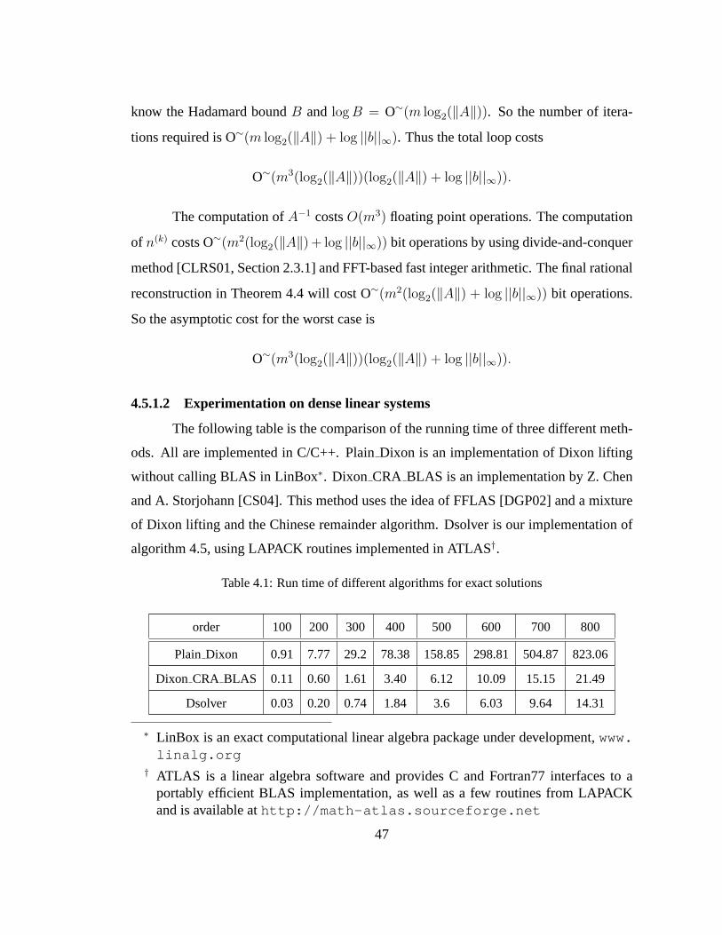
know the Hadamard boundB and log B = O∼(m log2(‖A‖)). So the number of itera-

tions required is O∼(m log2(‖A‖) + log ||b||∞). Thus the total loop costs

O∼(m3(log2(‖A‖))(log2(‖A‖) + log ||b||∞)).

The computation ofA−1 costsO(m3) floating point operations. The computation

of n(k) costs O∼(m2(log2(‖A‖) + log ||b||∞)) bit operations by using divide-and-conquer

method [CLRS01, Section 2.3.1] and FFT-based fast integer arithmetic. The final rational

reconstruction in Theorem 4.4 will cost O∼(m2(log2(‖A‖) + log ||b||∞)) bit operations.

So the asymptotic cost for the worst case is

O∼(m3(log2(‖A‖))(log2(‖A‖) + log ||b||∞)).

4.5.1.2 Experimentation on dense linear systems

The following table is the comparison of the running time of three different meth-

ods. All are implemented in C/C++. PlainDixon is an implementation of Dixon lifting

without calling BLAS in LinBox∗. Dixon CRA BLAS is an implementation by Z. Chen

and A. Storjohann [CS04]. This method uses the idea of FFLAS [DGP02] and a mixture

of Dixon lifting and the Chinese remainder algorithm. Dsolver is our implementation of

algorithm 4.5, using LAPACK routines implemented in ATLAS†.

Table 4.1: Run time of different algorithms for exact solutions

order 100 200 300 400 500 600 700 800

Plain Dixon 0.91 7.77 29.2 78.38 158.85 298.81 504.87 823.06

Dixon CRA BLAS 0.11 0.60 1.61 3.40 6.12 10.09 15.15 21.49

Dsolver 0.03 0.20 0.74 1.84 3.6 6.03 9.64 14.31

∗ LinBox is an exact computational linear algebra package under development,www.linalg.org

† ATLAS is a linear algebra software and provides C and Fortran77 interfaces to aportably efficient BLAS implementation, as well as a few routines from LAPACKand is available athttp://math-atlas.sourceforge.net

47

In the table above, times are in seconds. Tests are sequentially run on a server with

3.2GHZ Intel Xeon processors and 6GB memory. All entries are integers randomly and

independently chosen from[−220, 220]. Clearly, both Dsolver and DixonCRA BLAS

benefit from high performance BLAS routines implemented in ATLAS and are much

faster than PlainDixon. Our algorithm is easier to be implemented than the idea used in

Dixon CRA BLAS. Also, Dsolver is faster than DixonCRA BLAS. The reason can be

explained as follows. Dixon lifting and our method need near2 log(det(A))log p

and 2 log(det(A))log α

iterations, respectively, wherep is the base ofp-adic lifting andα is the geometric average

of α(i). For a well-conditioned matrix, theα(i) ≥ 230 in each iteration. That is, in each

iteration, Dsolver can get at least30 binary leading bits of the exact solution ofAx = r(i).

While in Dixon CRA BLAS, using Dixon lifting and FFLAS, each iteration in Dixon

lifting can only get ap-adic digit,p < 227. This is because arithmetic operations such as

multiplication in Zp must be done exactly in double precision floating point arithmetic.

So our method is expected to use fewer iterations. Also, our method can directly call

BLAS routines without any extra cost for conversion between integer and floating point

representation. Then it is not surprising that Dsolver is faster than DixonCRA BLAS.

4.5.2 An exact rational solver for sparse integer linear systems

The main idea is to apply algorithm 4.5 by replacing the numerical solver with a

successful sparse linear system solver. In the case of sparse matrices (including structured

matrices and general sparse matrices), the algorithm can be especially fast if a sparse nu-

merical solver works for the matrix at hand. Iterative methods such as Lanczos method,

or Jacobi’s method, the generalized minimum residual method (with restarts), conjugate

gradient method, and bi-conjugate gradient method (- see e.g. [Saa03, TB97]]) are good

candidates for numerically solving sparse linear systems. If the matrices are general

sparse matrices with many zero entries, sparse elimination methods such as SuperLU

are good candidates too. It is not our purpose to examine these issues, such as choice

48

of preconditioner, associated with sparse numerical solvers. But we point out that when

the chosen numerical solver does succeed, then our method can get the exact solution

extremely rapidly. In next section, our example from Trefethen’s challenge suite shows a

case where an iterative method works after applying a custom preconditioner adapted to

the specific matrix.

4.6 An application to a challenge problem

We will demonstrate that our new method can run about 720 times faster than

previous methods. In 2002, Prof. L. N. Trefethen posted “A Hundred-dollar, Hundred-

digit Challenge” at SIAM News, Volume 35, Number 1. We are particularly interested in

problem 7. Here is the original problem:

Let A be the20, 000× 20, 000 matrix whose entries are zero everywhereexcept for the primes2, 3, 5, 7, ..., 224737 along the main diagonal and thenumber1 in all the positionsaij with |i − j| = 1, 2, 4, 8, ..., 16384. What isthe(1, 1) entry ofA−1?

Though only the first10 decimal digits are required for the original problem, in 2002,

anexact(symoblic) solution was computed by Jean-Guillaume Dumas of LMC-IMAG in

Grenoble, France. It is a fraction with exactly 97,389 digits each for relatively prime

numerator and denominator. He ran 182 processors for four days using Wiedemann’s

algorithm [Wie86] and the Chinese remainder algorithm - see [DTW02] for details. A

few months later, we verified the result on one processor supporting 64-bit architecture

with a large main memory(8GB) usingp-adic lifting [Dix82] after explicitly computing

the inverse ofA mod a word size prime by Gaussian elimination and storing it as a dense

matrix - see [DTW02] for details. Now, armed with the main idea presented here, the

exact answer of this problem can be computed in25 minutes with a PC with Linux,

1.9GHZ Pentium processor, 1GB memory, or in 13 minutes with a better machine with

dual 3.2GHZ Intel Xeon processors and 6GB memory. And only a few MB of memory

at run time are required. Our new method has won us an entry in the update followup of

49

a book [BLWW04] discussing the solutions to the challenge problems. This method is

an application of our main idea with a custom approximate inverse of the input matrix.

The generaln × n matrix with the same pattern asA is a sparse matrix with O(n log n)

non-zero entries and is almost a row diagonally dominant matrix except in the first few

rows. For the special20000 × 20000 matrix A, there are at most29 non-zero entries in

each row (column). So, if we represent the matrix as a block matrix:

A =

A11 A12

A21 A22

,

whereA11, A12, A21, A22 are500× 500, 500× 19500, 19500× 500, and19500× 19500

matrices, respectively. ThenA22 is astrongly diagonally dominantmatrix. LetD be the

diagonal part ofA22, E be the rest. Therefore,

||A

A11 0

A21 D

−1

− I||∞ = ||(

A11 0

A21 D

+

0 A12

0 E

)

A11 0

A21 D

−1

− I||∞

= ||[−A12D

−1A21A−111 A12D

−1 − ED−1A21A−111 ED−1

]||∞

.

We know all diagonal entries ofA22 are greater than3571 (which is the500th prime),

all off-diagonal entries ofA22 are0 or 1, and there are at most28 non-zero off-diagonal

entries ofA22 in each row or column, so||ED−1||∞ ≤ 357128

< 1127.5

. AlsoA12 andA21 are

very sparse, and every diagonal entry ofD is larger than3571. Therefore it is reasonable

to estimate that||A

A11 0

A21 D

−1

− I||∞ is less than164

, near twice of 1127.5

, and follow-

up computation shows that164

is not overestimated. So we can use

A11 0

A21 D

−1

as an

approximate inverse ofA. Note that it is a lower triangle block matrix. Thus we can

quickly solve A11 0

A21 D

x = y, for anyy.

We call LAPACK routines to compute the inverse ofA11 explicitly, and store it as a dense

matrix. Other parts can be stored as sparse matrices and be used as blackboxes. Here, in

50

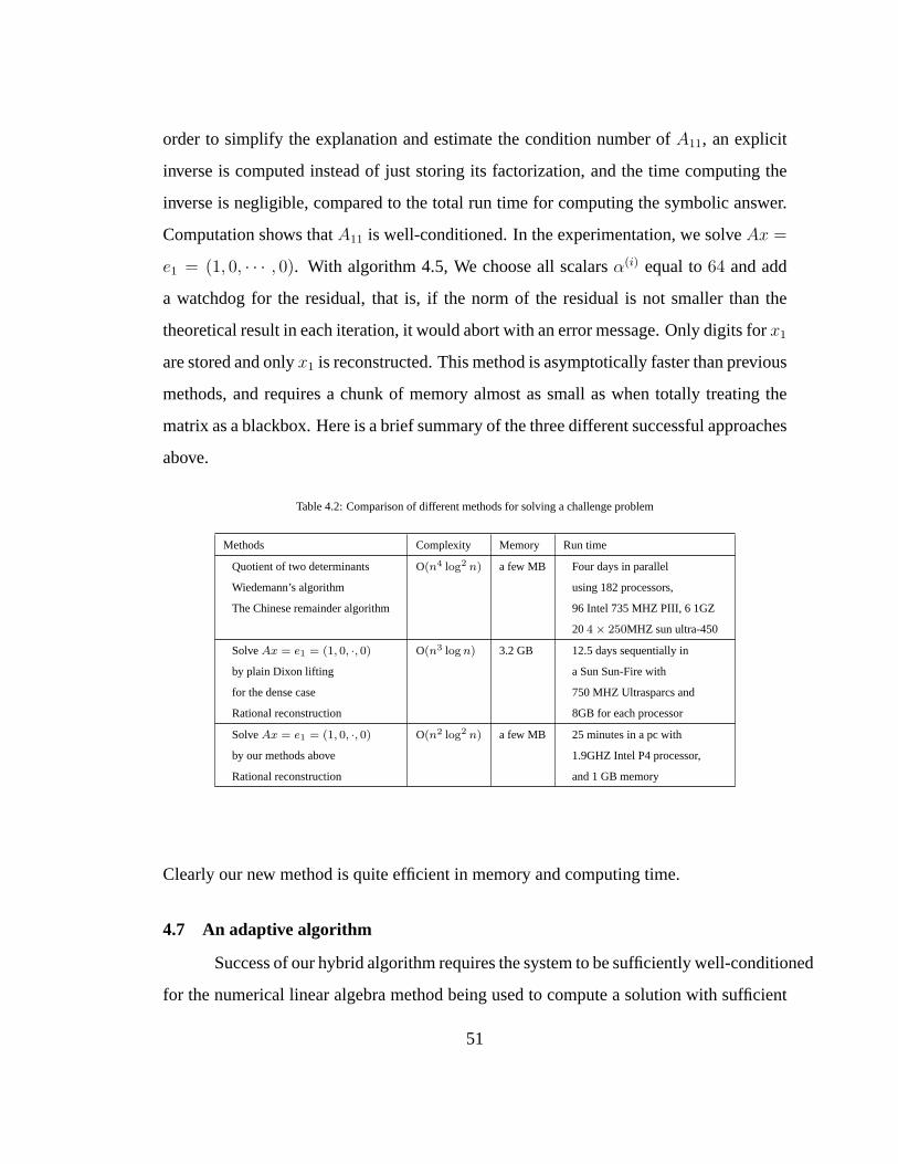
order to simplify the explanation and estimate the condition number ofA11, an explicit

inverse is computed instead of just storing its factorization, and the time computing the

inverse is negligible, compared to the total run time for computing the symbolic answer.

Computation shows thatA11 is well-conditioned. In the experimentation, we solveAx =

e1 = (1, 0, · · · , 0). With algorithm 4.5, We choose all scalarsα(i) equal to64 and add

a watchdog for the residual, that is, if the norm of the residual is not smaller than the

theoretical result in each iteration, it would abort with an error message. Only digits forx1

are stored and onlyx1 is reconstructed. This method is asymptotically faster than previous

methods, and requires a chunk of memory almost as small as when totally treating the

matrix as a blackbox. Here is a brief summary of the three different successful approaches

above.

Table 4.2: Comparison of different methods for solving a challenge problem

Methods Complexity Memory Run time

Quotient of two determinants

Wiedemann’s algorithm

The Chinese remainder algorithm

O(n4 log2 n) a few MB Four days in parallel

using 182 processors,

96 Intel 735 MHZ PIII, 6 1GZ

204× 250MHZ sun ultra-450

SolveAx = e1 = (1, 0, ·, 0)

by plain Dixon lifting

for the dense case

Rational reconstruction

O(n3 log n) 3.2 GB 12.5 days sequentially in

a Sun Sun-Fire with

750 MHZ Ultrasparcs and

8GB for each processor

SolveAx = e1 = (1, 0, ·, 0)

by our methods above

Rational reconstruction

O(n2 log2 n) a few MB 25 minutes in a pc with

1.9GHZ Intel P4 processor,

and 1 GB memory

Clearly our new method is quite efficient in memory and computing time.

4.7 An adaptive algorithm

Success of our hybrid algorithm requires the system to be sufficiently well-conditioned

for the numerical linear algebra method being used to compute a solution with sufficient

51

accuracy. It aborts quickly on ill-conditioned cases.p-adic lifting [Dix82, MC79] works

on both well-conditioned and ill-conditioned cases. In practice, it runs slower than our

hybrid algorithm. An adaptive algorithm can be formed easily, starting with our hybrid

algorithm and switching top-adic lifting if it aborts. This adaptive algorithm is imple-

mented in the LinBox library.

52

Chapter 5

COMPUTATION OF SMITH FORMS OF INTEGER MATRICES

5.1 Introduction

Smith normal form (Smith form, in short) plays an important role in the study of

algebraic group theory, homology group theory, systems theory, matrix equivalence, Dio-

phantine systems, theory of control. In 1861, H. J. Smith introduced the Smith normal

form. Since then, the Smith form problem has attracted the attention of many researchers

due to its wide application. Many algorithms have been discovered and algorithmic com-

plexity has been improved. With computer power nowadays, the Smith form of dimension

one thousand can be computed in a few hours. One of our main contributions to Smith

form computation is that we discovered an engineered algorithm for Smith normal form

which yields very good practical run time and asymptotic complexity. Asymptotically

fast algorithms may run slowly in practice. There are choices of algorithms and each is

favored by certain cases. Moreover, different parts of Smith form are favored by different

algorithms. Based on both theoretical and experimental results, we propose an “engi-

neered” Smith form algorithm. Another contribution of ours is that we have improved the

probability bound of an important Monte-Carlo algorithm. Also, we have discovered an

efficient preconditioner for computing the Smith normal form.

This chapter will start with a history of Smith form algorithms. Algorithms in

[KB79, Ili89, HM91, Sto96, Gie96, EGV00, KV03] will be discussed. Then in section

5.6, we will present our algorithm for dense matrix Smith form, which primarily takes the

form of a suite of improvements to the probabilistic algorithm in [EGV00]. Finally, an

“engineered” Smith form algorithm will be introduced.

53

5.2 The definition of Smith form

The following definition of Smith form is based on the existence proof by H. Smith

in [Smi61].

DEFINITION 5.1. For every integer matrixA, there exist unimodular matricesU and

V , and a diagonal matrixS with non-negative diagonal entriessi, for i = 1, · · · , n. such

that A = USV , andsi|si+i. The matrixS is called the Smith Normal Form or simply

Smith Form ofA, thesi are called the invariant factors ofA. Here an integer matrix is

called unimodular if and only if its determinant is1 or−1.

REMARK.Note that the choices ofU andV are not unique, though the Smith Normal

FormS of an integer matrixA is unique.

The following is a simple fact about Smith form.

FACT 5.2. If A is a givenn×n integer matrix with invariant factors(s1, ..., . . . , sn), then

det(A) = ±∏

0≤i≤n

si, andsi = 0, if i > rank(A).

For an integer matrixA, we definesi(A) to be theith invariant factor ofA. In spite

of the abstract definition of Smith form, the Smith form can be computed via a series of

elementary column and row operations consisting of (see e.g. [New72]):

1. Adding an integer multiple of one row (column) to another.

2. Multiplying a row (column) by -1.

3. Swapping two rows (columns).

For example, a2× 2 matrix:

A =

1 1

1 3

.

54

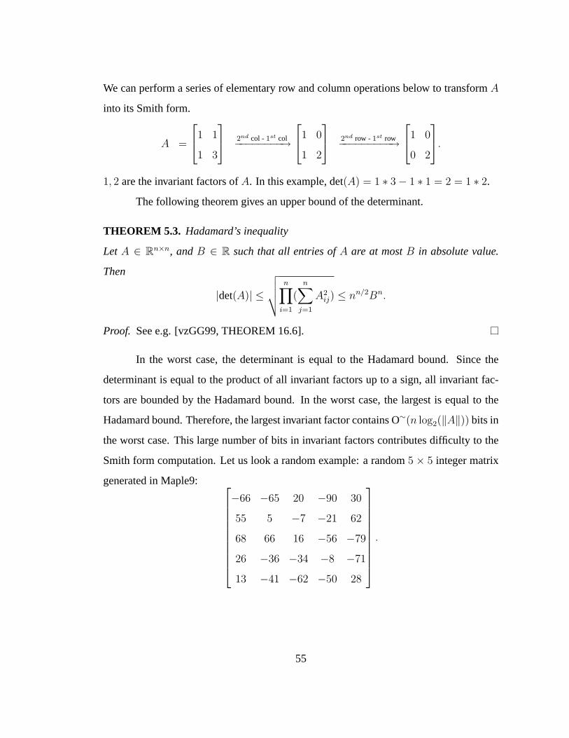
We can perform a series of elementary row and column operations below to transformA

into its Smith form.

A =

1 1

1 3

2nd col - 1st col−−−−−−−−→

1 0

1 2

2nd row - 1st row−−−−−−−−−→

1 0

0 2

.

1, 2 are the invariant factors ofA. In this example, det(A) = 1 ∗ 3− 1 ∗ 1 = 2 = 1 ∗ 2.

The following theorem gives an upper bound of the determinant.

THEOREM 5.3. Hadamard’s inequality

Let A ∈ Rn×n, andB ∈ R such that all entries ofA are at mostB in absolute value.

Then

|det(A)| ≤

√√√√ n∏i=1

(n∑

j=1

A2ij) ≤ nn/2Bn.

Proof. See e.g. [vzGG99, THEOREM 16.6].

In the worst case, the determinant is equal to the Hadamard bound. Since the

determinant is equal to the product of all invariant factors up to a sign, all invariant fac-

tors are bounded by the Hadamard bound. In the worst case, the largest is equal to the

Hadamard bound. Therefore, the largest invariant factor contains O∼(n log2(‖A‖)) bits in

the worst case. This large number of bits in invariant factors contributes difficulty to the

Smith form computation. Let us look a random example: a random5 × 5 integer matrix

generated in Maple9:

−66 −65 20 −90 30

55 5 −7 −21 62

68 66 16 −56 −79

26 −36 −34 −8 −71

13 −41 −62 −50 28

.

55

Its Smith formS by SmithForm in LinearAlgebra package in Maple9 is:

1 0 0 0 0

0 1 0 0 0

0 0 1 0 0

0 0 0 1 0

0 0 0 0 4820471082

.

Though the random matrix itself has order 5 and small entries, its Smith form has

a large entry.

In the following, a number of Smith form algorithms will be discussed. The fol-

lowing notations will be used. We useAi to denote theith column of a matrixA and use

COL(i)(ROW(i)) to denote theith column(row) of matrix.

5.3 Kannan and Bachem’s algorithm

As pointed out by Frumkin in [Fru77], none of the algorithms given before 1979

for computing the Smith Normal Form of an integer matrix is known to be a polynomial

time algorithm. In 1997, X. Fang and G. Havas [FH97] showed there is an elimination

algorithm for the Smith form of an integer matrix with an exponential time complexity

and exponential space required in a worst case.

In 1979, R. Kannan and A. Bachem [KB79] proved that there was a polynomial

time algorithm for the Smith form of an integer matrix. Their method successively con-

trols the size of the entries of the integer matrix after each elimination step by using the

extended greatest common divisor and special elimination.

Here I will explain the algorithm in non-singular cases with every leading prin-

cipal minor nonsingular. The general case can be transformed into this case by matrix

permutation and a standard row reduction technique - see [KB79].

The essential part of Kannan and Bachem’s method is a special extended gcd-

based row (column) elimination, which eliminates an off-diagonal entry in a column

(row).

56

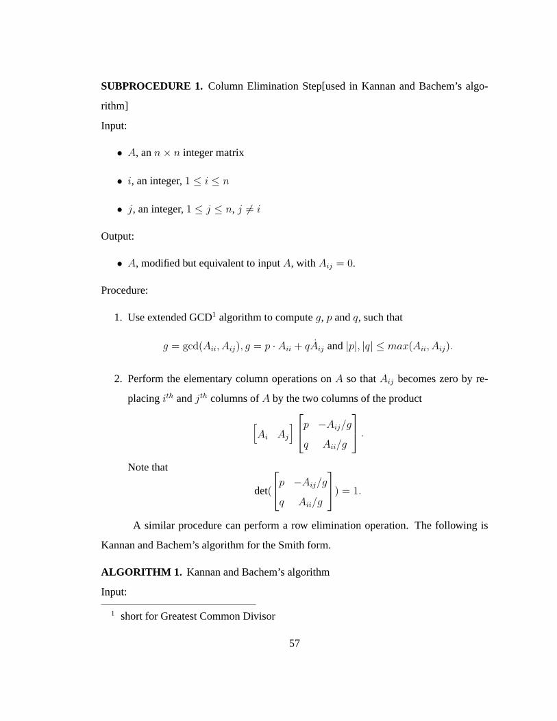
SUBPROCEDURE 1. Column Elimination Step[used in Kannan and Bachem’s algo-

rithm]

Input:

• A, ann× n integer matrix

• i, an integer,1 ≤ i ≤ n

• j, an integer,1 ≤ j ≤ n, j 6= i

Output:

• A, modified but equivalent to inputA, with Aij = 0.

Procedure:

1. Use extended GCD1 algorithm to computeg, p andq, such that

g = gcd(Aii, Aij), g = p · Aii + qAij and|p|, |q| ≤ max(Aii, Aij).

2. Perform the elementary column operations onA so thatAij becomes zero by re-

placingith andjth columns ofA by the two columns of the product

[Ai Aj

] p −Aij/g

q Aii/g

.

Note that

det(

p −Aij/g

q Aii/g

) = 1.

A similar procedure can perform a row elimination operation. The following is

Kannan and Bachem’s algorithm for the Smith form.

ALGORITHM 1. Kannan and Bachem’s algorithm

Input:

1 short for Greatest Common Divisor

57

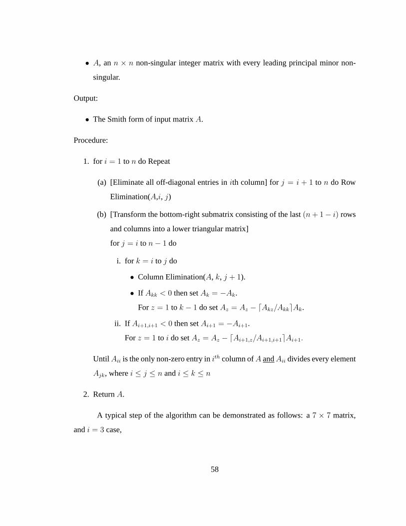
• A, ann × n non-singular integer matrix with every leading principal minor non-

singular.

Output:

• The Smith form of input matrixA.

Procedure:

1. for i = 1 to n do Repeat

(a) [Eliminate all off-diagonal entries inith column] forj = i + 1 to n do Row

Elimination(A,i, j)

(b) [Transform the bottom-right submatrix consisting of the last(n + 1− i) rows

and columns into a lower triangular matrix]

for j = i to n− 1 do

i. for k = i to j do

• Column Elimination(A, k, j + 1).

• If Akk < 0 then setAk = −Ak.

For z = 1 to k − 1 do setAz = Az − dAkz/AkkeAk.

ii. If Ai+1,i+1 < 0 then setAi+1 = −Ai+1.

For z = 1 to i do setAz = Az − dAi+1,z/Ai+1,i+1eAi+1.

Until Aii is the only non-zero entry inith column ofA andAii divides every element

Ajk, wherei ≤ j ≤ n andi ≤ k ≤ n

2. ReturnA.

A typical step of the algorithm can be demonstrated as follows: a7 × 7 matrix,

andi = 3 case,

58

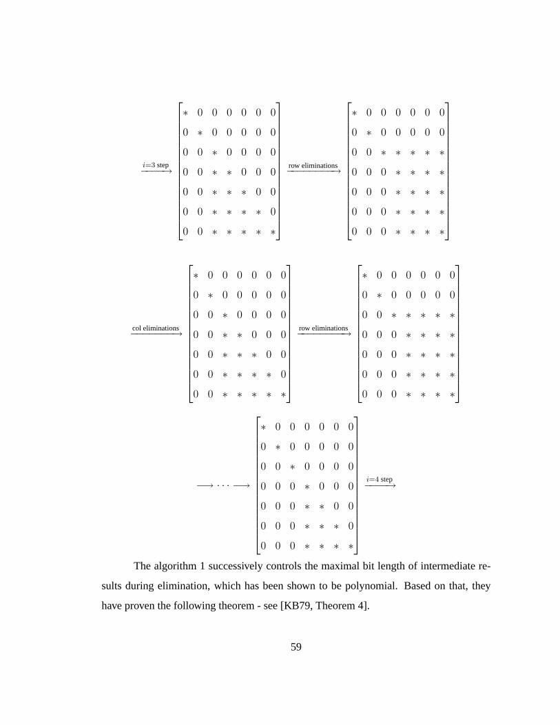
i=3 step−−−−→

∗ 0 0 0 0 0 0

0 ∗ 0 0 0 0 0

0 0 ∗ 0 0 0 0

0 0 ∗ ∗ 0 0 0

0 0 ∗ ∗ ∗ 0 0

0 0 ∗ ∗ ∗ ∗ 0

0 0 ∗ ∗ ∗ ∗ ∗

row eliminations−−−−−−−−→

∗ 0 0 0 0 0 0

0 ∗ 0 0 0 0 0

0 0 ∗ ∗ ∗ ∗ ∗

0 0 0 ∗ ∗ ∗ ∗

0 0 0 ∗ ∗ ∗ ∗

0 0 0 ∗ ∗ ∗ ∗

0 0 0 ∗ ∗ ∗ ∗

col eliminations−−−−−−−→

∗ 0 0 0 0 0 0

0 ∗ 0 0 0 0 0

0 0 ∗ 0 0 0 0

0 0 ∗ ∗ 0 0 0

0 0 ∗ ∗ ∗ 0 0

0 0 ∗ ∗ ∗ ∗ 0

0 0 ∗ ∗ ∗ ∗ ∗

row eliminations−−−−−−−−→

∗ 0 0 0 0 0 0

0 ∗ 0 0 0 0 0

0 0 ∗ ∗ ∗ ∗ ∗

0 0 0 ∗ ∗ ∗ ∗

0 0 0 ∗ ∗ ∗ ∗

0 0 0 ∗ ∗ ∗ ∗

0 0 0 ∗ ∗ ∗ ∗

−→ · · · −→

∗ 0 0 0 0 0 0

0 ∗ 0 0 0 0 0

0 0 ∗ 0 0 0 0

0 0 0 ∗ 0 0 0

0 0 0 ∗ ∗ 0 0

0 0 0 ∗ ∗ ∗ 0

0 0 0 ∗ ∗ ∗ ∗

i=4 step−−−−→

The algorithm 1 successively controls the maximal bit length of intermediate re-

sults during elimination, which has been shown to be polynomial. Based on that, they

have proven the following theorem - see [KB79, Theorem 4].

59

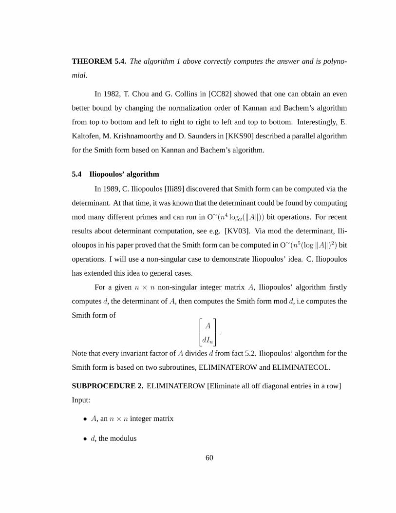
THEOREM 5.4. The algorithm 1 above correctly computes the answer and is polyno-

mial.

In 1982, T. Chou and G. Collins in [CC82] showed that one can obtain an even

better bound by changing the normalization order of Kannan and Bachem’s algorithm

from top to bottom and left to right to right to left and top to bottom. Interestingly, E.

Kaltofen, M. Krishnamoorthy and D. Saunders in [KKS90] described a parallel algorithm

for the Smith form based on Kannan and Bachem’s algorithm.

5.4 Iliopoulos’ algorithm

In 1989, C. Iliopoulos [Ili89] discovered that Smith form can be computed via the

determinant. At that time, it was known that the determinant could be found by computing

mod many different primes and can run in O∼(n4 log2(‖A‖)) bit operations. For recent

results about determinant computation, see e.g. [KV03]. Via mod the determinant, Ili-

oloupos in his paper proved that the Smith form can be computed in O∼(n5(log ‖A‖)2) bit

operations. I will use a non-singular case to demonstrate Iliopoulos’ idea. C. Iliopoulos

has extended this idea to general cases.

For a givenn × n non-singular integer matrixA, Iliopoulos’ algorithm firstly

computesd, the determinant ofA, then computes the Smith form modd, i.e computes the

Smith form of A

dIn

.

Note that every invariant factor ofA dividesd from fact 5.2. Iliopoulos’ algorithm for the

Smith form is based on two subroutines, ELIMINATEROW and ELIMINATECOL.

SUBPROCEDURE 2. ELIMINATEROW [Eliminate all off diagonal entries in a row]

Input:

• A, ann× n integer matrix

• d, the modulus

60

• ρ, a row index, and1 ≤ ρ ≤ n.

Output:

• A, modified but equivalent, with properties,Aρi = 0, for ρ < i ≤ n.

Procedure:

1. [MakeAρρ = 0] If Aρρ 6= 0 then

• computer, x1, x2, such that

r = gcd(Aρρ, Aρ,ρ+1), r = x1 Aρρ + x2 Aρ,ρ+1, |x1| ≤ |aρ,ρ+1|/2,

and|x2| ≤ |aρρ|/2.

• Update theρthand(ρ + 1)th columns to become

[Aρ A(ρ+1)

] aρ,ρ+1/r x1

−arhoρ/r x2

.

2. computes, andtj, ρ + 1 ≤ j ≤ n such that

s = gcd(Aρ,ρ+1, · · · , Aρn), ands =n∑

j=ρ+1

tjAρj.

3. set

tj := tj (mod d), for ρ + 1 ≤ j ≤ n.

4. update

COL(ρ)← COL(ρ) +n∑

j=ρ+1

tiCOL(j).

5. Forρ + 1 ≤ j ≤ n, update

COL(j)← COL(j)− (Aρj/s)COL(ρ).

61

6. NormalizeAjρ by modd, for ρ + 1 ≤ j ≤ n

REMARK.This subroutine eliminates off diagonal entries in a row. The transformation

is equivalent to multiplying

A

dIn

by a unimodular integer matrix on the left.

There is a similar subroutine ELIMINATECOL, which eliminates off diagonal

entries in a column.

ALGORITHM 2. Iliopoulos’ algorithm

Input:

• A, ann× n non-singular matrix.

Output:

• The Smith form ofA.

Procedure:

1. [Compute the determinant]d← the determinant ofA.

2. [TransformA to an equivalent diagonal matrix] Forρ = 1 to n do Repeat[Finding

a right pivoting]

- ELIMINATEROW (A, d, ρ)

- ELIMINATECOL (A, d, ρ)

Until

aρρ | aρj, for all ρ + 1 ≤ j ≤ n.

3. [Compute the Smith form of the diagonal matrix] forp = 1 to n do for q = p + 1

to n do

- h← App

62

- app ← GCD(App, h)

- aqq ← Aqqh/app

4. ReturnA.

REMARK.The Smith form of a diagonal matrix can be efficiently computed via a special

sorting network - see section 5.7.1.

Iliopoulos’ algorithm above uses the determinant to control the maximal bit length

of entries of intermediate results during elimination.

THEOREM 5.5. For an n × n non-singular matrixA, the algorithm 2 above correctly

computes its Smith form and requiresO∼(n5(log2(‖A‖))2) bit operations.

REMARK.The exponent5 in the complexity can be explained as follows:3 comes from

the exponent part in Gaussian elimination,1 comes from the loop in order to find the right

pivoting, and another1 comes from the bit length of the modulus. Thus, an elimination-

based optimal algorithm will require O∼(n4 log2(‖A‖)) bit operations to compute the

Smith form of ann× n integer matrix.

Proof. See [Ili89, corollary 5.3].

In 1991, J. Hafner and K. McCurley [HM91] independently discovered an idea

similar to Iliopoulos’ above for the Smith form computation.

5.5 Storjohann’s near optimal algorithm

In 1996, A. Storjohann [Sto96] improved the complexity substantially. He showed

that the Smith form can be computed in O∼(n(ω+1) log2(‖A‖)) bit operations. This algo-

rithm computes the Smith form modulo the determinant by using matrix multiplication.

The important step of computing Smith form via elimination is the choice ofU

andV . This algorithm emphasizes the choice ofU andV . The essential part of this

method is banded matrix reduction.

63

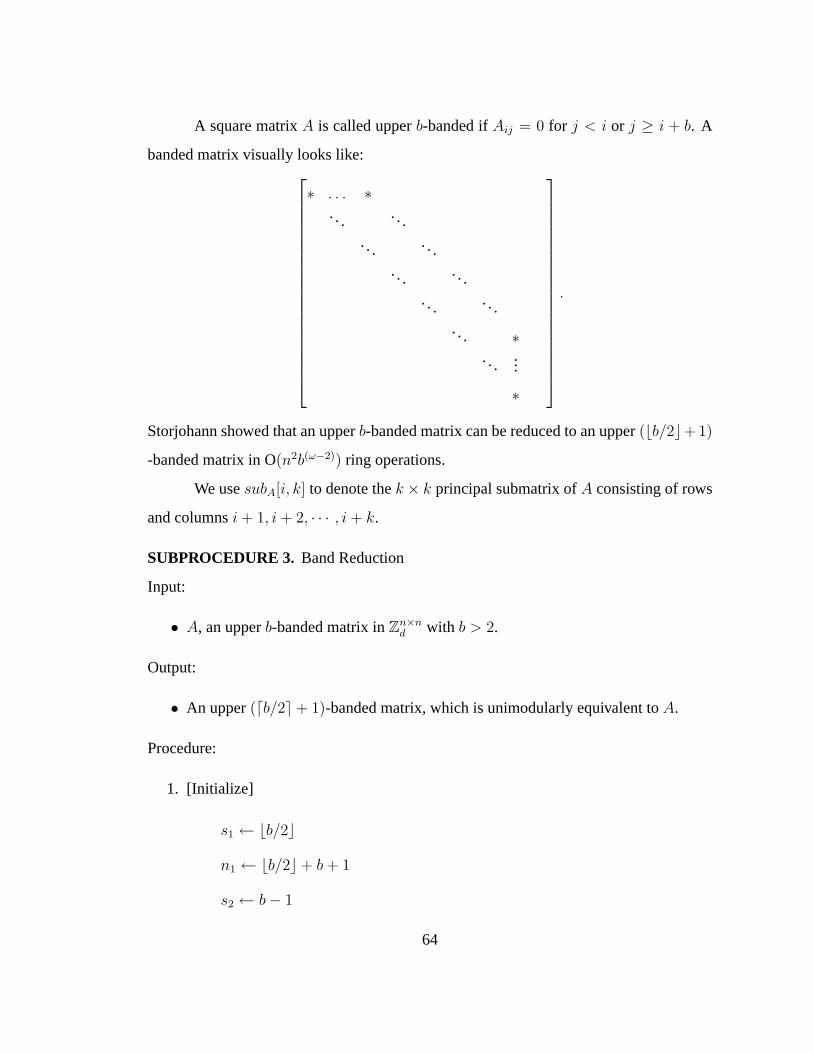
A square matrixA is called upperb-banded ifAij = 0 for j < i or j ≥ i + b. A

banded matrix visually looks like:

∗ . . . ∗... .. .

.. . .. ... . .. .

.. . .. ... . ∗

.. ....

∗

.

Storjohann showed that an upperb-banded matrix can be reduced to an upper(bb/2c+1)

-banded matrix in O(n2b(ω−2)) ring operations.

We usesubA[i, k] to denote thek × k principal submatrix ofA consisting of rows

and columnsi + 1, i + 2, · · · , i + k.

SUBPROCEDURE 3. Band Reduction

Input:

• A, an upperb-banded matrix inZn×nd with b > 2.

Output:

• An upper(db/2e+ 1)-banded matrix, which is unimodularly equivalent toA.

Procedure:

1. [Initialize]

s1 ← bb/2c

n1 ← bb/2c+ b + 1

s2 ← b− 1

64

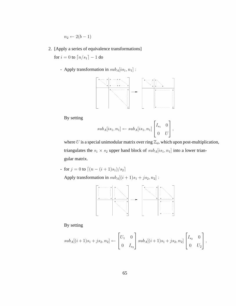
n2 ← 2(b− 1)

2. [Apply a series of equivalence transformations]

for i = 0 to dn/s1e − 1 do

- Apply transformation insubA[is1, n1] :

By setting

subA[is1, n1]← subA[is1, n1]

Is1 0

0 U

,

whereU is a special unimodular matrix over ringZd, which upon post-multiplication,

triangulates thes1 × s2 upper hand block ofsubA[is1, n1] into a lower trian-

gular matrix.

- for j = 0 to d(n− (i + 1)s1)/s2e

Apply transformation insubA[(i + 1)s1 + js2, n2] :

By setting

subA[(i + 1)s1 + js2, n2]←

U1 0

0 Is2

subA[(i + 1)s1 + js2, n2]

Is2 0

0 U2

,

65

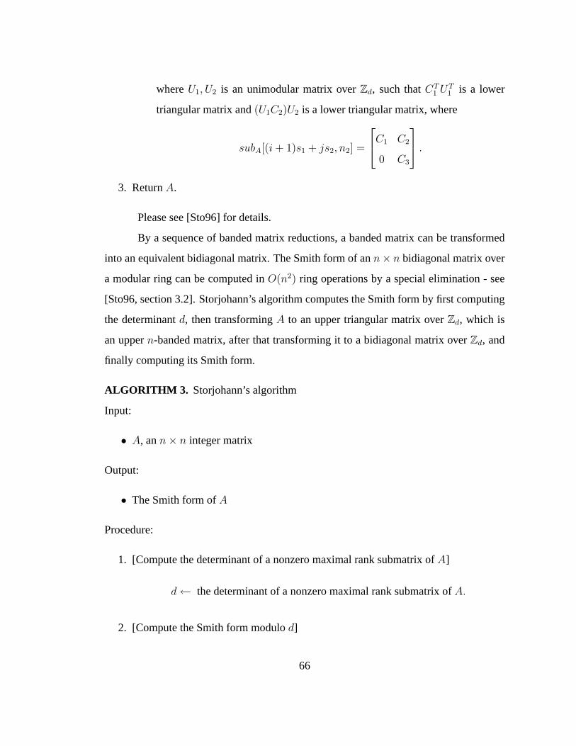
whereU1, U2 is an unimodular matrix overZd, such thatCT1 UT

1 is a lower

triangular matrix and(U1C2)U2 is a lower triangular matrix, where

subA[(i + 1)s1 + js2, n2] =

C1 C2

0 C3

.

3. ReturnA.

Please see [Sto96] for details.

By a sequence of banded matrix reductions, a banded matrix can be transformed

into an equivalent bidiagonal matrix. The Smith form of ann× n bidiagonal matrix over

a modular ring can be computed inO(n2) ring operations by a special elimination - see

[Sto96, section 3.2]. Storjohann’s algorithm computes the Smith form by first computing

the determinantd, then transformingA to an upper triangular matrix overZd, which is

an uppern-banded matrix, after that transforming it to a bidiagonal matrix overZd, and

finally computing its Smith form.

ALGORITHM 3. Storjohann’s algorithm

Input:

• A, ann× n integer matrix

Output:

• The Smith form ofA

Procedure:

1. [Compute the determinant of a nonzero maximal rank submatrix ofA]

d← the determinant of a nonzero maximal rank submatrix ofA.

2. [Compute the Smith form modulod]

66

3. Compute a unimodular matrixU overZd, such thatUT × AT is a lower triangular

matrix overZd.

4. SetA← A× U [Note thatA is n-banded matrix now]

5. b← n

6. whileb > 2 do [TransformA into a bidiagonal matrix]

A← Band Reduction(A, b),

and

b← db/2 + 1e.

7. [Compute the Smith form of Bidiagonal matrix overZd.]

A← the Smith Normal Form ofA.

8. ReturnA.

THEOREM 5.6. For ann× n integer matrix, algorithm 3 above correctly computes its

Smith form and requiresO∼(n4 log2(‖A‖)) bit operations.

Proof. See [Sto96, Theorem 14].

5.6 Eberly, Giesbrecht, and Villard’s algorithm with improvements

All algorithms I discussed above are deterministic. Storjohann’s algorithm 3 is

the near optimal deterministic algorithm for Smith form. One question is whether the

algorithmic complexity can be improved if randomization is allowed. The answer isyes.

In the coming few sections, we will discuss a few probabilistic algorithms.

In 2000, W. Eberly, M. Giesbrecht and G. Villard [EGV00] discovered a new

approach to compute the Smith form of ann× n integer matrixA in O∼(n3.5 log ‖A‖) or

O∼(n2+ω/2 log2(‖A‖)) when fast matrix multiplication is available. The largest invariant

67

factor of a non-singular integer matrix can be computed by symbolically solving a few

linear systems. the invariant factor of any index can be computed by means of random

perturbations. A binary search can be used to find all distinct invariant factors.

5.6.1 Largest invariant factor with a “bonus” idea

This algorithm is a variation of the algorithm [EGV00, LargestInvariantFactor].

Our contribution is the “bonus” idea which can be used to find the second largest invariant

factor with very little extra work.

ALGORITHM 4. LargestInvariantFactor

Input:

• A, a non-singularn× n integer matrix.

• ε, an error probability requirement.

Output:

• sn, the largest invariant factor ofA with probability at least1− ε.

• sn−1, the second largest invariant factor ofA.

Procedure:

1. M := 6 + 2n(log2 n + log2(‖A‖));L := 0, . . . ,M − 1.

2. Sets(0)n := 1; s

(0)n−1 := 0.

3. SetN := dlog(1/ε)/ log 1.5e.

4. Fori from 1 to N do

a. Choose random vectors,~b(2i−1), and~b(2i) ∈ Ln.

b. SolveA~x(2i−1) = ~b(2i−1) andA~x(2i) = ~b(2i) over the rational field.

68

c. Compute

t(2i−1) := lcm(denom(~x(2i−1)1 ), . . . , denom(~x(2i−1)

n ))

and

t(2i) := lcm(denom(~x(2i)1 ), . . . , denom(~x(2i)

n )).

d. Computeu(i) = gcd(t(2i−1),t(2i))

s2(

[t(2i−1)~x(2i−1) t(2i)~x(2i)

])

. [[t(2i−1)~x(2i−1) t(2i)~x(2i)

]is

ann× 2 integer matrix. ]

e. Computes(i)n := lcm(s

(i−1)n , t(2i−1), t(2i)).

f. Computes(i)n−1 = gcd(s

(i−1)n−1 , u(i)).

5. s(N)n ands

(N)n−1.

REMARK.In addition to the largest invariant factor, algorithm 4 also computes the second

largest invariant with expected extra O∼(n2 log2(‖A‖)) bit operations. The extra cost is

negligible, comparing to the total cost. This is the reason we call it “bonus”. This is

important in practice, since big prime factors often occur only in the largest invariant

factor. For example, the random matrices have trivial invariant factors, i.e. all invariant

factors are1 except the largest invariant. Also the (second) largest invariant factor can be

used to improve Iliopoulos’ algorithm and Storjohann’s, by replacing determinant with

(second) largest invariant factor. In practice, the largest invariant factor is often smaller

than the determinant, and the second largest is smaller still.

THEOREM 5.7. Given ann × n non-singular integer matrixA and an error boundε,

algorithm 4 above computes the largest invariant factor ofA with probability at least

1 − ε and the second largest factor ofA with probability near1 −√

ε. The algorithm is

expected to run in

O∼(n3 log2(‖A‖) log(1/ε))

bit operations.

69

Proof. By [EGV00, Theorem 2.1], we know in each iterationi, t(2i−1) andt(2i) are always

factors ofsn and

Prob(lcm(t(2i−1), t(2i)) 6= sn) < 2/3.

After repeatingN times, the error probability is at mostε.

The reason thats(N)n−1 is equal to the second largest invariant factor can be explained

below. It is known thatsn(A)A−1 is an integer matrix, and the Smith form ofsn(A)A−1

is

diag(sn(A)

sn(A),

sn(A)

sn−1(A), · · · , sn(A)

s1(A)).

SoSn−1(A) = sn(A)s2(sn(A)A−1)

. If we group the rational vectors~b and solutions~x in the loop

into pairs,

A~x(2i−1) = ~b(2i−1) andA~x(2i) = ~b(2i),

then

sn(A)A−1[~b(2i−1),~b(2i)

]=

[sn(A)~x(2i−1), sn(A)~x(2i)

].

Thus

sn−1(A) =sn(A)

s2([sn(A)~x(2i−1), sn(A)~x(2i)])=

gcd(t(2i−1), t(2i))

s2([t(2i−1)~x(2i−1), t(2i)~x(2i)]).

For any primep, following from lemma 5.17, an approach like in theorem 5.14 shows that

Prob(p -sn−1(A)

s2([sn(A)~x(2i−1), sn(A)~x(2i)])) ≥ (1− 1

MdM

pe)(1− (

1

MdM

pe)2).

So Prob(s(N)n−1 6= sn−1(A)) is near

√ε. Moreover the computedsn−1(A) is always a factor

of the true answer.

Each iteration requires O∼(n3 log2(‖A‖)) bit operations. So the number of ex-

pected bit operations for the algorithm is O∼(n3 log2(‖A‖) log(1/ε)).

5.6.2 The invariant factor of any index with a new efficient perturbation

Algorithm [EGV00, Algorithm:OneInvariantFactor] can be used to obtain the in-

variant factor of any index by means of perturbation. Forn × i random matrixU and

70

i × n random matrixV , the largest invariant factor ofA + UV is likely to be theith

invariant factor ofA. We propose a more efficient perturbation. LetL′ andR′ be random

matrices with each entry randomly and independently chosen from a set of integers. Then

the largest invariant factor of [Ii L′

]A

Ii

R′

is likely to be theith invariant factor ofA. Also the “bonus” idea in algorithm 4 can be

extended here to compute the preceding invariant factor.

ALGORITHM 5. OneInvariantFactor

Input:

• A, ann×m integer matrix, w.l.g.m ≤ n.

• i, an integer,2 ≤ i ≤ rank(A).

• ε, an error probability requirement.

Output:

• si, theith invariant factor ofA with probability at least1− ε.

• si−1, the(i− 1)th invariant factor ofA.

Procedure:

1. Sets(0)i := 0.

2. Sets(0)i−1 := 0.

3. SetS := 210d i(6 log n+3 log2(‖A‖))210

e; L = [0, . . . , S − 1].

4. SetN := log(10/ε)/ log(24/23);

5. for j = 1 to N do

71

a. Choose random integer matrixL ∈ Li×(n−i).

b. Choose random integer matrixR ∈ L(m−i)×i.

c. ComputeA′ =[Ii L

]A

Ii

R

.

d. Compute(t(j), u(j)), the largest and the second largest invariant factors ofA′,

by algorithm 4.

e. Computes(j)i := gcd(s

(j−1)i , t(j)); s

(j)i−1 := gcd(s

(j−1)i−1 , u(j)).

6. returns(N)i , ands

(N)i−1.

REMARK.The algorithm is similar to algorithm in [EGV00, section 3]. But only one

random set is used here and more efficient preconditioners are used. Also we are going to

prove a better theoretical probability bound.

THEOREM 5.8. For a givenn× n integer matrix and2 ≤ i ≤ rank(A), the algorithm

5 above computes theith invariant factor ofA with probability at least1 − ε and the

(i− 1)th invariant factor with probability near1−√

ε. The algorithm is expected to run

in

O∼(in2 log2(‖A‖) log2(1/ε))

bit operations.

We need a few lemmas and theorems described below in order to prove this theo-

rem.

5.6.2.1 Non-uniformly distributed random variables

In this subsection, we focus on non-uniformly distributed random variables over a

finite fieldF with additional bound condition,

α ≤ Prob(x = d) ≤ β, ∀d ∈ F.

72

If α = β = 1p, thenx is a uniformly distributed random variable. The next lemma

describes an example.

LEMMA 5.9. If an integerx which is uniformly randomly chosen from[0, . . . , S − 1], is

mapped to a finite fieldZp, then

1

SbSpc ≤ Prob(x = d mod p) ≤ 1

SdSpe

for anyd ∈ Zp. Thusx mod p is a non-uniformly distributed random variable overZp.

Proof. Given an integerd and primep, there is at mostdSpe integersx such that,

0 ≤ x ≤ S − 1, andx = d (mod p).

So

Prob(x = d mod p) ≤ 1

SdSpe.

By similarly reasoning,

Prob(x = d mod p) ≤ 1

SbSpc.

The next lemma characterizes the distribution of dot products for a random vector.

LEMMA 5.10. Given a non-zero vector~t ∈ F and an elementd ∈ F, if ~x = (x1, . . . , xn)

is a random vector inFn with each entry independently and non-uniformly randomly

chosen fromF with the probability that any element inF ranging fromα to β is chosen,

then

α ≤ Prob(~x : ~t · ~x = d) ≤ β.

Proof. Prob(~x : ~t · ~x = d) ≤ β. can be proved by using the variation of Schwartz-Zippel

lemma in [Gie01, lemma]. Also it can be argued by a simple idea, which can be used to

prove the inequality in the left side.

73

Since~t = (t1, . . . , tn) 6= 0, without loss of generality we assumet1 6= 0.

Prob(~x : ~t · ~x = d)

=∑

j∈F Prob((x2, . . . , xn) :∑n

i=2 tixi = j)Prob(x1 : x1 = d−jt1|∑n

i=2 tixi = j)

=∑

j∈F Prob((x2, . . . , xn) :∑n

i=2 tixi = j)Prob(x1 : x1 = d−jt1

)

≤∑

j∈F βProb((x2, . . . , xn) :∑n

i=2 tixi = j)

= β.

By similarly reasoning, we knowα ≤ Prob(~x : ~t · ~x = d).

The lemma below characterizes the distribution of a random null space vector.

LEMMA 5.11. Given a matrixA ∈ Fn×m with rankr, if ~x = (x1, . . . , xm)T is a random

vector inF with each entry independently and non-uniformly randomly chosen fromF

with the probability that any element inF ranging fromα to β is chosen, then

αr ≤ Prob(~x : Ax = 0) ≤ βr.

Proof. We know∃L, U, P , such thatA = LUP , P is permutation matrix,L is non-

singular, andU has the shape Ir U ′

0 0

.

Thus,

Prob(~x : Ax = 0)

= Prob(~x : LUPx = 0)

= Prob(~x : LUPx = 0)

= Prob(~x : Ux = 0)

= Prob((x1, . . . , xr)T = −U ′(xr+1, . . . , xn)T )

=∏r

j=1 Prob(xj = −U ′j (xr+1, . . . , xn)T |xk = −U ′

k (xr+1, . . . , xn)T ,∀k, k < j)

=∏r

j=1 Prob(xj = −U ′j (xr+1, . . . , xn)T )

≤ βr

74

By similarly reasoning,

αr ≤ Prob(~x : Ax = 0).

More generally, for a givenb ∈ Fm, if under the same hypotheses, then

Prob(~x : Ax = b) ≤ βr.

Furthermore, ifAx = b has a solution. then

Prob(~x : Ax = b) ≥ αr.

The next lemma characterizes the distribution of a random vector in a sub-space.

LEMMA 5.12. Given ak−dimensional subspace ofFn, S = Span(S1, . . . , Sk). If ~x =

(x1, . . . , xn)T is a random vector inFN with each entry independently and non-uniformly

randomly chosen fromF with the probability that any element inF ranging fromα to β is

chosen, then

αn−k ≤ Prob(~x : x ∈ S) ≤ βn−k.

Proof. We extend(S1, . . . , Sk) to be a basis ofFn, (S1, . . . , Sn). Let B = (S1, . . . , Sn).

Then

Prob(~x : ~x ∈ S) = Prob(B−1k+1,...,n~x = 0) ≤ βn−k.

By similarly reasoning,

αn−k ≤ Prob(~x : ~x ∈ S).

The next lemma characterizes the distribution of a random non-singular matrix.

THEOREM 5.13. Given ann×n matrixB overF, if R is ann×n random matrix over

F with each entry independently and non-uniformly chosen fromF with the probability

that any particular element inF is chosen being no more thanβ, then

Prob(det(R−B) 6= 0) ≥∞∏i=1

(1− βi).

75

Proof. We will only prove the case whereB = 0 case, sinceB 6= 0 is result of thisB = 0

case and lemma 5.10 If we letR = (R1, . . . , Rn), then det(A) 6= 0 if and only if

ai /∈ Span(R1, . . . , Ri−1),∀i, 1 ≤ i ≤ n.

Thus,

Prob(det(R) 6= 0)

=∏n

i=1 Prob(Ri /∈ Span(R1, . . . , Ri−1)|R1, . . . , Ri−1 are linearly independent.)

≥∏n

i=1(1− βn+1−i)

≥∏∞

i=1(1− βi).

.

For the case whereB = 0 , there is a similar result in [MS04]. Note that in the

uniform case, we haveβ = 1p, thus

Prob(det(R) 6= 0) ≥∞∏i=1

(1− (1

p)i).

If β < 1, then∏∞

i=1(1− βi) converges and is positive. Moreover,

∞∏i=1

(1− βi) = e∑∞

i=1 ln(1−βi) ≥ e∑∞

i=1(−βi) ≥ e−β1−β ≥ 1− β

1− β.

The next lemma characterizes the distribution of a perturbation.

THEOREM 5.14. Given ann × n matrix T and anm × n matrix B over F with

rank(

T

B

) = n, if R is ann × n random matrix overF with each entry independently

and non-uniformly chosen fromF with the probability that any element inF is chosen no

more thanβ, then

Prob(R : det(T + RB) 6= 0) ≥∞∏i=1

(1− βi).

76

Proof. If we let r = rank(B), then there exists ann×n non-singular matrixQ, such that

BQ =[B′ 0

],

whereB′ is of full column rank. Let us we rewrite

TQ =[T1 T2

],

whereT1 andT2 aren× r andn× (n− r) matrices, respectively.Q is non-singular, so

n = rank(

T

B

) = rank(

TQ

BQ

) = rank(

T1 T2

B′ 0

).

Thus rank(T2) = n− r. Therefore there exists non-singularM , such that,

MTQ =

T11 0

T21 T22

andT22 is non-singular,

whereT11, T21 andT22 arer× r, r× (n− r), and(n− r)× (n− r) matrices, respectively.

Let us look at

M(T + RB)Q = MTQ + MRBQ =

T11 + M1RB′ 0

∗ T22

.

Therefore

det(T + RB) 6= 0 if and only det(T11 + M1RB′) 6= 0,

sinceM , Q, andT22 are all non-singular.

Note thatM1 is fully row ranked andB′ is fully column ranked. There exist

permutation matrices,P1 andP2, such that thei× i leading principle minors ofM1P1 and

P2B′ are non-singular. LetR′ = P T

1 RP T2 . ThenP1RB′ = M1P1R

′P2B′. If we represent

M1P1 =[M11 M12

], P2B

′ =[B11 B12

], R′ =

R11 R12

R21 R22

.

Then

T11 + M1RB′ = M11(R11 + Res(R12, R21, R22, M11, T11, B11)B11),

77

where

Res(R12, R21, R22, M11, T11, B11) = M−111 (T11+M12B21B11+M11R22B12+M12R22B12)B

−111 .

Since bothM11 andB11 are non-singular,T11 + M1RB′ is non-singular if and only if

det(R11 + Res(R12, R21, R22, T11, M11, B11) 6= 0.

So det(T + RB) 6= 0 if and only if

det(R11 + Res(R12, R21, R22, T11, M11, B11) 6= 0.

Thus

Prob(R : det(R11 + Res(R12, R21, R22, T11, M11, B11) 6= 0)

=∑

C1,C2,C3Prob(R11 : det(R11 + Res(C1, C2, C3, T11, M11, B11) 6= 0

|R12 = C1, R21 = C2, R22 = C3)Prob(R12 = C1, R21 = C2, R22 = C3)

=∑

C1,C2,C3Prob(R11 : det(R11 + Res(C1, C2, C3, T11, M11, B11) 6= 0)

Prob(R12 = C1, R21 = C2, R22 = C3)

Therefore, by theorem 5.13,

Prob(R : det(R11 + Res(R12, R21, R22, T11, M11, B11) 6= 0)

≥∑

C1,C2,C3.∏∞

i=1(1− βi)Prob((R12 = C1, R21 = C2, R22 = C3)

≥∏∞

i=1(1− βi).

.

So

Prob(R : det(T + RB) 6= 0) ≥∞∏i=1

(1− βi).

Note that ifT andB aren × n andm × n matrices overF, respectively, and if

there existsR, such thatT + RB is non-singular, then

rank(

T

B

) ≥ rank([I R

] T

B

) ≥ rank(T + RB) = n.

78

Thus

rank(

T

B

) = n.

COROLLARY 5.15. Given a primep, under the same assumption in the theorem above

aboutT andB, if R is ann× n random integer matrix with each entry independent and

uniformly chosen from[0, . . . , S − 1], then

Prob(det(T + RB) 6= 0 mod p) ≥∞∏i=1

(1− (1

SdSpe)i).

Proof. This follows from theorem 5.14 and fact 5.9.

The lemma below explores the relationship between invariant factors of the per-

turbation and those of the original matrix.

LEMMA 5.16. If L andA are l×n andn×m integer matrices, respectively, thensi(LA)

is always a multiple ofsi(A), for all 1 ≤ i ≤ min(l,m, n).

Proof. If si(A) = 0, then rank(A) < i. so

rank(LA) ≤ rank(A) < i.

Thussi(LA) = 0.

If si(A) = 1, obviously the lemma is true.

Otherwise, let us have a look at the Smith form ofLA andA modsi(A). Suppose

thatA overZsi(A) has the Smith form

S = diag(s1, . . . , sr, 0, . . . , 0), for somer < i.

So there exist corresponding integer matricesU andV , such that both det(U ) and det(V )

are coprime tosi(A) andA = USV . Therefore,

si(LA) = si(LUSV ) = si(

L′11S11 0

0 0

V ) (mod si(A)),

79

whereL′11, S11 are the firstr× r principal sub-matrices ofLU andS, respectively. Since

det(V ) is coprime tosi(A) andr < i, we know

si(

L′11S11 0

0 0

V ) = si(

L′11S11 0

0 0

) = 0 (mod si(A)).

This meanssi(LA) is a multiple ofsi(A).

The lemma below explores the sufficient condition ofp - si(LA)si(A)

, wherep is a

prime.

LEMMA 5.17. If A is ann × m integer matrix,p is a prime, andi is an integer, such

that si(A) 6= 0, then there exists a full column ranked matrixM , such that for anyi × n

integer matrixL,

p -si(LA)

si(A), if det(LM) 6= 0 (mod p).

Proof. Let us look at the local Smith form ofA at primep. There exist integer matrices

U , V andD, such that,

A = UDV, det(U) 6= 0 (mod p), and det(V ) 6= 0 (mod p), and

D is the local Smith form ofA atp.

We rewriteU , D as block matrices,

U =[M M ′

], D =

D1 0

0 D2

,

whereM is ann× i matrix,D1 is ani× i matrix. Then

LA =[LMD1 LM ′D2

]V.

Note that the entries ofD2 are multiples of those inD1. So If det(LM) 6= 0 mod p, then

D1 is the local Smith form ofLA atp, i.e. p - si(LA)si(A)

. Also,M has full column rank.

80

5.6.2.2 Proof of Theorem 5.8

Based on lemmas and theorems above, we are able to prove theorem 5.8.

Proof. If si(A) = 0, then

si([Ii L

]A

Ii

R

) = 0, for anyL andR.

Therefore the theorem is true.

Otherwisesi(A) 6= 0. If L is a randomi×(n−i) matrix with each entry uniformly

and independently chosen from integer set[0, ..., S−1], then by lemma 5.17 and corollary

5.15,

Prob(L : p -si([IiL]A)

si(A)) ≥

∞∏i=1

(1− (1

SdSpe)i), for any primep.

If prime p ≥ S, then1

SdSpe =

1

S.

And if 11 ≤ p < S, then1

SdSpe ≤ 1

p+

1

S.

Also, we chooseS divisible by2, 3, 5, and7. Thus

Prob(L : p -si([IiL]A)

si(A)) ≥

1− 1

S−1, if p ≥ S

1− 1.12(1p

+ 1

S ), if 11 ≤ p < S√

25

, if p = 2

12, if p = 3

34, if p = 5

56, if p = 7

Note that ∏∞i=1(1− (1

p+ 1

S )i) ≥ 1−1p+ 1

S1− 1

p− 1

S

> 1−1p+ 1

S1− 1

11− 1

210

> 1− 1.12(1p

+ 1

S ).

81

Therefore, afterN = log(10/ε)/ log(24/23) number of iterations, the computedith in-

variant factor ofA,

Prob(s(N)i 6= si(A)) ≤ (23

24)N + (3

4)N + ( 7

16)N + (11

36)N + 5.5(4.5

10)N−1

≤ 10(2324

)N−1 ≤ ε.

So algorithm 5 computes theith invariant factor with probability at least1 − ε. By sim-

ilarly reasoning, the second largest invariant factor is computed by the bonus idea with

probability with probability near1−√

ε.

In algorithm 5, each iteration costs

O∼(in2 + i3(log n + log2(‖A‖)) · log(1/ε)).

So the total cost will be

O∼(in2 + i3(log n + log2(‖A‖)) · log(1/ε)) log(1/ε)).

5.6.3 Binary search for invariant factors

The next lemma gives an upper bound for the number of distinct invariant factors

of an integer matrix.

LEMMA 5.18. LetA be ann× n integer matrix. ThenA has at most

O(n1/2(log n + log2(‖A‖))1/2)

distinct invariant factors.

Proof. See e.g. [EGV00, Theorem 4.1]. Or the non-singular case can simply be proved by

the argument below. SupposeA has invariant factorss1, . . . , sn, andk distinct invariant

factorssi1 , . . . , sik in increasing order. We know

k∏j=1

sij ≤n∏

j=1

sn = |det(A)|.

82

Also, 2sij ≤ sij+1, for all 1 ≤ j ≤ k − 1. SoSij ≥ 2j−1. Thus

|det(A)| ≥k∏

j=1

sij ≥k∏

j=1

2j−1 = 2j(j−1)/2.

Therefore,A has at most O(√

log |det(A)|) distinct invariant factors. By the Hadamard

bound,|det(A)| ≤ nn/2(log2(‖A‖))n. SoA has at most

O(n1/2(log n + log2(‖A‖))1/2).

The proof can be modified to handle the singular case as well.

Algorithm 5 can be used to compute the invariant factor of any index. A binary

search for every distinct invariant factor is feasible. Without loss of generality, we assume

thatA is ann×m integer matrix, andm ≤ n.

THEOREM 5.19. Given an× n integer matrix and error boundε, there exists a proba-

bilistic algorithm which computes the Smith form ofA with probability at least1− ε, and

is expected to run in

O∼(n3.5(log2(‖A‖))1.5 log2(1/ε))

bit operations.

Proof. See [EGV00, THEOREM 4.2].

5.7 Smith form algorithms for sparse matrices

Though the chapter focuses on the Smith form of dense matrices, some inter-

esting algorithms for sparse cases are helpful to form an “engineered” Smith form al-

gorithm. In 1996, M. Giesbrecht [Gie96] showed the Smith form can be computed in

O∼(n2E log2(‖A‖)) bit operations, whereE is the number of non-zero entries ofA. This

algorithm is based on computation of determinantal divisorsdi, which are the greatest

common divisor of all thei × i minors ofA. Determinantal divisors are computed by

83

the characteristic polynomials over the integers. Note that theith invariant factor ofA is

equal todi/di−1 (let d0 = 1), or 0 if di = 0.

In 2000, J. Dumas, B. Saunders and G. Villard [DSV00] showed an interesting

valence algorithm, which requires O∼(n2E log2(‖A‖)) bit operations plus the time for

factoring the valences. Firstly the valencev, which is the trailing nonzero coefficient of

the minimal polynomial ofAT A, is computed. The valence will give information about

the primes which may occur in invariant factors. Then the valencev is factored to find

each prime which may occur in invariant factors. For each primep|v, Sp, the Smith

form of A over the local ringZ(p) =⋃∞

i=1 Zpi, is computed. Note that the Smith form

of A =∏

p|v Sp. The valence algorithm succeeds in many examples, especially those in

computation of homology groups. Dumas, Heckenbach, Saunders and Welker developed

a Gap homology package, which is available atwww.eecis.udel.edu/˜linbox/

gap.html . In the next subsection, we will discuss the Smith form of a diagonal matrix

which is a very special sparse matrix.

5.7.1 Smith forms of diagonal matrices

Iliopoulos’ elimination produces an equivalent diagonal matrix. Computation of

the Smith form of this diagonal matrix is rather straightforward usingn2 (extended) gcd

computations[Ili89], a cost that is much lower than the elimination to diagonal form.

Nonetheless, in this section we present a faster method to compute the Smith form of a

diagonal matrix. It is soft linear in the size of the input. This speedup may be significant

in some settings. In any case, it is an interesting and easily implemented method.

Given a matrixA = diag(a1, . . . , an) we show how to compute its Smith form.

Define the input size to beN =∑n

i=0(len(ai)), where len(a) = 1 + log(|a|). The run

time is soft linear inN , O∼(N). A basic observation is that

diag(a, b) is equivalent to diag(g, l), where

g = gcd(a, b) andl = lcm(a, b).

84

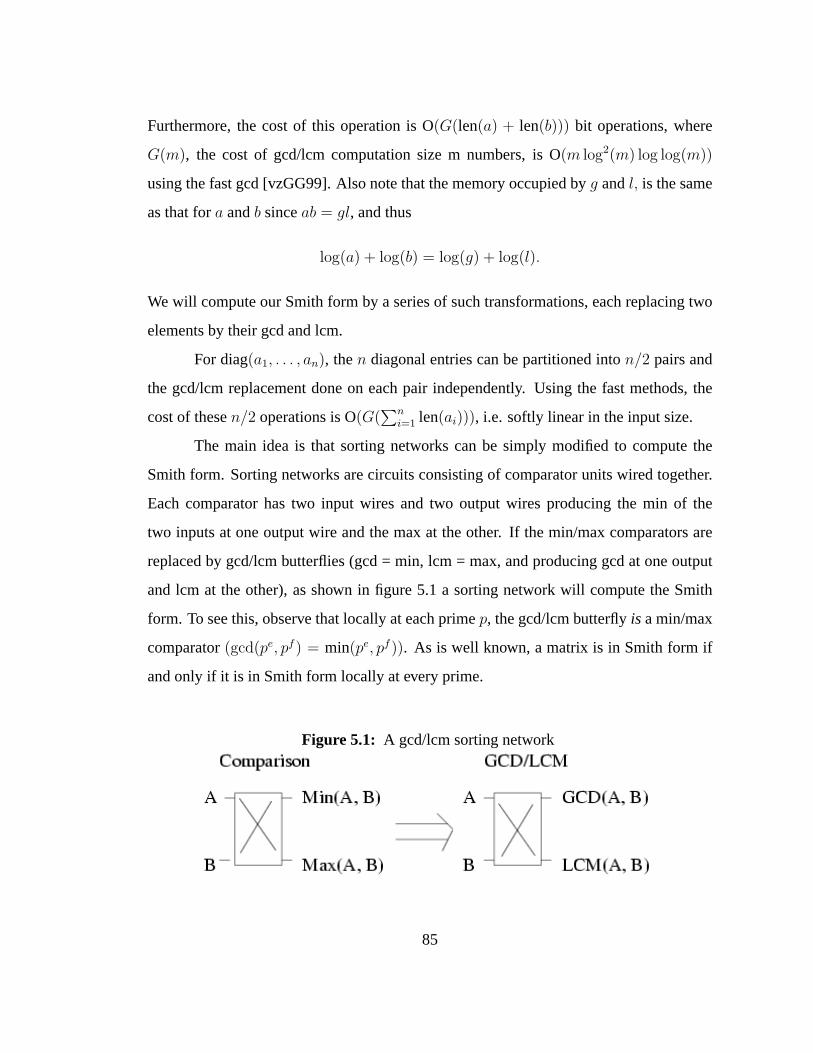
Furthermore, the cost of this operation is O(G(len(a) + len(b))) bit operations, where

G(m), the cost of gcd/lcm computation size m numbers, is O(m log2(m) log log(m))

using the fast gcd [vzGG99]. Also note that the memory occupied byg andl, is the same

as that fora andb sinceab = gl, and thus

log(a) + log(b) = log(g) + log(l).

We will compute our Smith form by a series of such transformations, each replacing two

elements by their gcd and lcm.

For diag(a1, . . . , an), then diagonal entries can be partitioned inton/2 pairs and

the gcd/lcm replacement done on each pair independently. Using the fast methods, the

cost of thesen/2 operations is O(G(∑n

i=1 len(ai))), i.e. softly linear in the input size.

The main idea is that sorting networks can be simply modified to compute the

Smith form. Sorting networks are circuits consisting of comparator units wired together.

Each comparator has two input wires and two output wires producing the min of the

two inputs at one output wire and the max at the other. If the min/max comparators are

replaced by gcd/lcm butterflies (gcd = min, lcm = max, and producing gcd at one output

and lcm at the other), as shown in figure 5.1 a sorting network will compute the Smith

form. To see this, observe that locally at each primep, the gcd/lcm butterflyis a min/max

comparator(gcd(pe, pf ) = min(pe, pf )). As is well known, a matrix is in Smith form if

and only if it is in Smith form locally at every prime.

Figure 5.1: A gcd/lcm sorting network

85

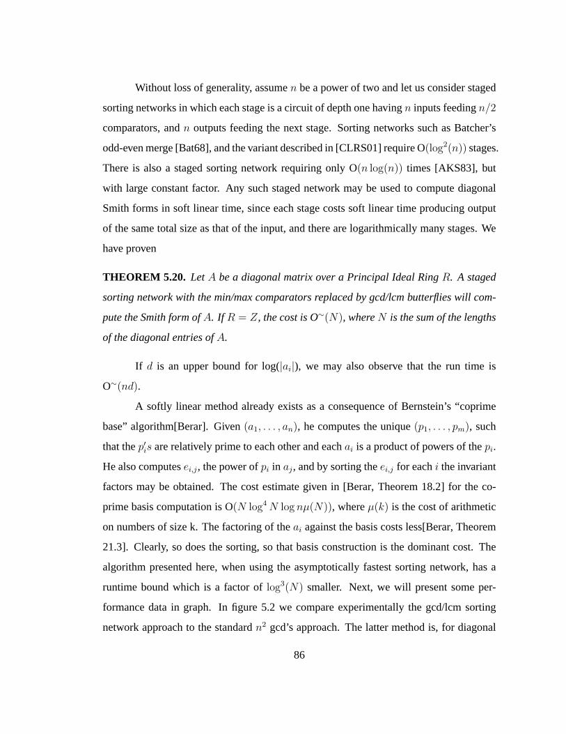
Without loss of generality, assumen be a power of two and let us consider staged

sorting networks in which each stage is a circuit of depth one havingn inputs feedingn/2

comparators, andn outputs feeding the next stage. Sorting networks such as Batcher’s

odd-even merge [Bat68], and the variant described in [CLRS01] require O(log2(n)) stages.

There is also a staged sorting network requiring only O(n log(n)) times [AKS83], but

with large constant factor. Any such staged network may be used to compute diagonal

Smith forms in soft linear time, since each stage costs soft linear time producing output

of the same total size as that of the input, and there are logarithmically many stages. We

have proven

THEOREM 5.20. Let A be a diagonal matrix over a Principal Ideal RingR. A staged

sorting network with the min/max comparators replaced by gcd/lcm butterflies will com-

pute the Smith form ofA. If R = Z, the cost is O∼(N), whereN is the sum of the lengths

of the diagonal entries ofA.

If d is an upper bound for log(|ai|), we may also observe that the run time is

O∼(nd).

A softly linear method already exists as a consequence of Bernstein’s “coprime

base” algorithm[Berar]. Given(a1, . . . , an), he computes the unique(p1, . . . , pm), such

that thep′is are relatively prime to each other and eachai is a product of powers of thepi.

He also computesei,j, the power ofpi in aj, and by sorting theei,j for eachi the invariant

factors may be obtained. The cost estimate given in [Berar, Theorem 18.2] for the co-

prime basis computation is O(N log4 N log nµ(N)), whereµ(k) is the cost of arithmetic

on numbers of size k. The factoring of theai against the basis costs less[Berar, Theorem

21.3]. Clearly, so does the sorting, so that basis construction is the dominant cost. The

algorithm presented here, when using the asymptotically fastest sorting network, has a

runtime bound which is a factor oflog3(N) smaller. Next, we will present some per-

formance data in graph. In figure 5.2 we compare experimentally the gcd/lcm sorting

network approach to the standardn2 gcd’s approach. The latter method is, for diagonal

86

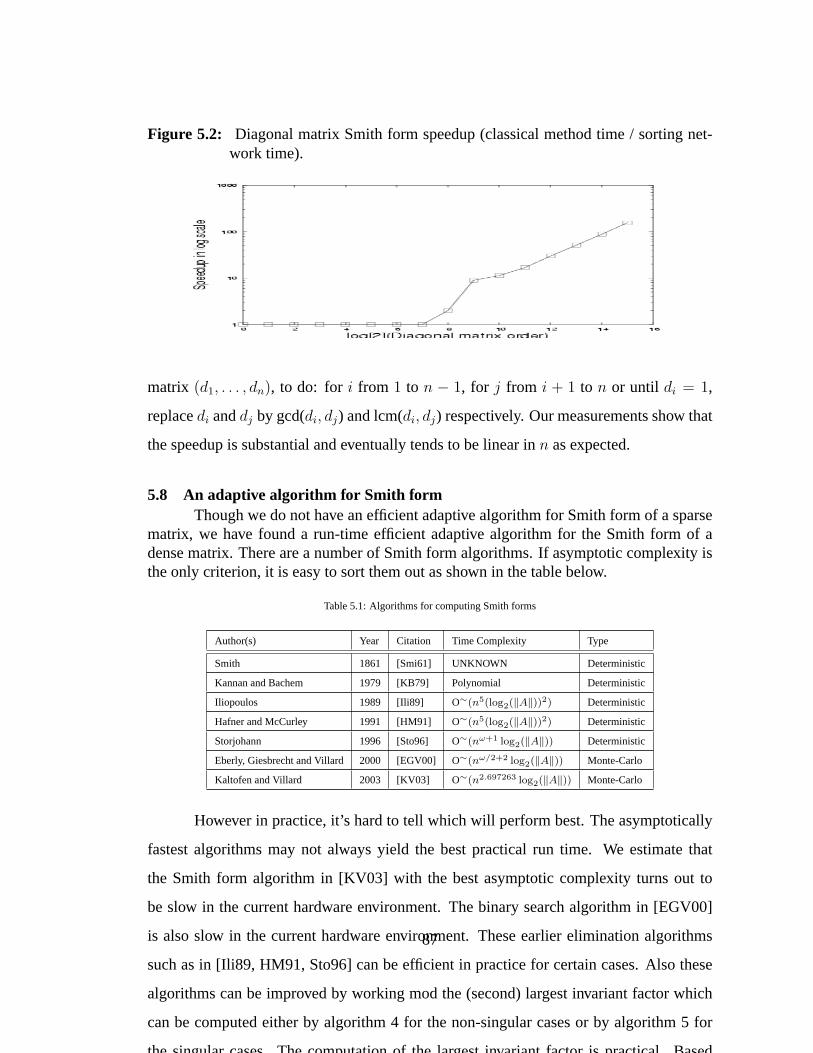
Figure 5.2: Diagonal matrix Smith form speedup (classical method time / sorting net-work time).

matrix (d1, . . . , dn), to do: for i from 1 to n − 1, for j from i + 1 to n or until di = 1,

replacedi anddj by gcd(di, dj) and lcm(di, dj) respectively. Our measurements show that

the speedup is substantial and eventually tends to be linear inn as expected.

5.8 An adaptive algorithm for Smith formThough we do not have an efficient adaptive algorithm for Smith form of a sparse

matrix, we have found a run-time efficient adaptive algorithm for the Smith form of adense matrix. There are a number of Smith form algorithms. If asymptotic complexity isthe only criterion, it is easy to sort them out as shown in the table below.

Table 5.1: Algorithms for computing Smith forms

Author(s) Year Citation Time Complexity Type

Smith 1861 [Smi61] UNKNOWN Deterministic

Kannan and Bachem 1979 [KB79] Polynomial Deterministic

Iliopoulos 1989 [Ili89] O∼(n5(log2(‖A‖))2) Deterministic

Hafner and McCurley 1991 [HM91] O∼(n5(log2(‖A‖))2) Deterministic

Storjohann 1996 [Sto96] O∼(nω+1 log2(‖A‖)) Deterministic

Eberly, Giesbrecht and Villard 2000 [EGV00] O∼(nω/2+2 log2(‖A‖)) Monte-Carlo

Kaltofen and Villard 2003 [KV03] O∼(n2.697263 log2(‖A‖)) Monte-Carlo

However in practice, it’s hard to tell which will perform best. The asymptotically

fastest algorithms may not always yield the best practical run time. We estimate that

the Smith form algorithm in [KV03] with the best asymptotic complexity turns out to

be slow in the current hardware environment. The binary search algorithm in [EGV00]

is also slow in the current hardware environment. These earlier elimination algorithms

such as in [Ili89, HM91, Sto96] can be efficient in practice for certain cases. Also these

algorithms can be improved by working mod the (second) largest invariant factor which

can be computed either by algorithm 4 for the non-singular cases or by algorithm 5 for

the singular cases. The computation of the largest invariant factor is practical. Based

on our experiments, the computation of largest invariant factor with4 rational solver

calls takes only about1/10 to 1/3 as long as the elimination step in typical non-singular

examples. Also, we found that the valence algorithm in [DSV00] should be favored for

87

certain matrices.

Both algorithm 4 and algorithm 5 are probabilistic algorithms and require a larger

number of iterations of symbolically solving non-singular linear systems to correctly

compute the largest invariant factor regarding small primes than they do regarding large

primes. For example, for a non-singular matrix,20 iterations of symbolically solving

non-singular linear systems are required in order to compute the power of2 occurring

in the largest invariant factor with probability of1 − 11000,000

, while only4 iterations are

expected to correctly compute the largest invariant with the same probability regarding

only primes bigger than100. We’ll do better to compute the contribution of small primes

and large primes in separate ways. To facilitate the discussion of this, we borrow from

number theory the terminology of smooth and rough numbers.

DEFINITION 5.21. Given a positive integerk, a number isk-smoothif it is a product of

primes smaller thank and isk-rough if it is a product of primes no less thank.

Given an integerk, every integeri can be written as a product of ak-smooth

number and ak-rough number.

Based this knowledge above, an “engineered” algorithm for Smith form is pro-

posed to deal with all cases. We called itengineeredbecause its structure is based on both

theoretical and experimental results. Different algorithms are suitable for different parts.

In particular, we discovered the importance of separating the rough part and smooth part

of invariant factors Therefore we divide the problem into smooth and rough sub-problems.

For each subproblem, we use adaptive algorithms to solve it based on thresholds, which

are determined by both theoretical and experimental results. The structure of the algo-

rithm has been influenced by classes of matrices we have encountered in practice. We

have designed it to recognize key patterns and go to the fastest practical algorithm for

those cases, while avoiding cases where this could go badly awry.

The algorithm begins, for matrixA, by computingr, the rank ofA, andd, the

degree of the minimal polynomial ofA or AAT . These can be done quite rapidly. The

88

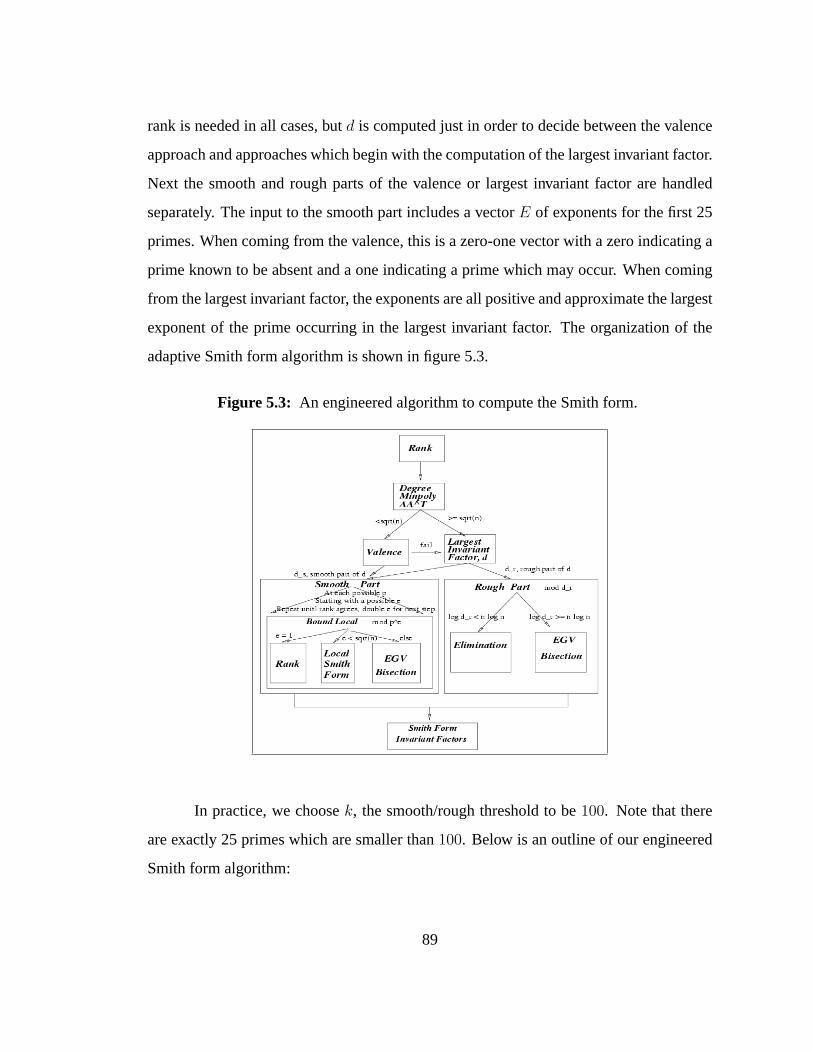
rank is needed in all cases, butd is computed just in order to decide between the valence

approach and approaches which begin with the computation of the largest invariant factor.

Next the smooth and rough parts of the valence or largest invariant factor are handled

separately. The input to the smooth part includes a vectorE of exponents for the first 25

primes. When coming from the valence, this is a zero-one vector with a zero indicating a

prime known to be absent and a one indicating a prime which may occur. When coming

from the largest invariant factor, the exponents are all positive and approximate the largest

exponent of the prime occurring in the largest invariant factor. The organization of the

adaptive Smith form algorithm is shown in figure 5.3.

Figure 5.3: An engineered algorithm to compute the Smith form.

In practice, we choosek, the smooth/rough threshold to be100. Note that there

are exactly 25 primes which are smaller than100. Below is an outline of our engineered

Smith form algorithm:

89

ALGORITHM 6. Engineered Smith form algorithm outline

Input:

• A, ann× n integer matrix.

• ε, an error probability requirement.

Output:

• S, vector of the invariant factors ofA. Monte Carlo with error probability at most

ε.

Procedure:

1. [rank] Computer = rank of A. This can be done rapidly by computing mod a

random prime from a suitable range. It is Monte Carlo with error probability at

mostε/2.

2. [minpoly degree] Compute the probable degree of the minimal polynomial ofAAT .

Computing the minimal polynomial mod a single random prime suffices for this

step. If this degree is less than a threshold go to the valence step, otherwise proceed

to the largest invariant factor step. We want a threshold less than√

n for asymptotic

complexity reasons. In practice the valence method is advantageous primarily when

the minimal polynomial degree is very low, so the threshold can be set lower than

that.

(a) [valence] Any prime that occurs in the invariant factors ofA occurs in the

valence (nonzero coefficient of lowest degree term) of the minimal polynomial

of A or AAT . It has been found in practice that some matrices of interest have

low degree minimal polynomials and rapidly computed valence forA orAAT .

See [DSV00] for further discussion of the valence method and for examples.

90

Compute one of these valences,v. If v is smooth, fori from 1 to 25, letEi

be 1 if thei-th prime dividesv, and be0 otherwise. Lett → 1, and go to the

smooth step. Otherwise the valence step fails, so proceed to largest invariant

factor step.

(b) [largest invariant factor] Compute the largest invariant factorsr and bonus, the

precedent invariant factor,sr−1, also using algorithm 5. The rough parts of the

bonus and of the largest invariant factor agree with the true values with high

probability. Thus the rough part of the bonus, often much smaller than the

rough part ofsr, can be used in the rough part step below. Lets be the smooth

part of the largest invariant factor fori from 1 to 25, letEi be one greater than

the exponent of thei-th prime insr, and lett be the remaining (rough) part of

sr.

3. [smooth part] LetSs → diag(1, . . . , 1), this will become the smooth part of the

Smith form. For i from 1 to 25, ifEi is positive, compute the local Smith form,Sp

at thei-th prime, and setSs → Ss ∗ Sp. The local Smith form atp is computed by

starting with the estimated exponente. If the number of non-zero invariant factors

in A (mod pe) is less than rank(A), doublee, repeat the computation until the

number of non-zero invariant factors modpe is equal to rank(A).

4. [rough part] ComputeSr the rough part of the Smith form by elimination if the

modulus is small, or by a binary search if not. Correct the rough part of the largest

invariant factor if necessary.

5. [return] Compute and returnS = Ss ∗ Sr. In practice,S, Ss, andSr may be repre-

sented as vectors (of the diagonal elements) or even as lists of the distinct entries

with their multiplicities.

The asymptotic complexity of the engineered algorithm above can be as good as the Smith

form algorithm in [EGV00]. We have following theorem.

91

THEOREM 5.22. There exist crossovers (thresholds) such that the engineered algorithm

can probabilistically compute the Smith form of ann× integer matrices inO∼(n3.5(log2(‖A‖))1.5)

bit operations.

Proof. In order to achieve O∼(n3.5(log2(‖A‖))1.5), we need to choose all crossovers such

that all parts can be computed in O∼(n3.5(log2(‖A‖))1.5). We choose the crossover be-

tween the valence and the largest invariant factor to be O∼(n0.5). Also we may choose

the crossovers between an elimination method and a binary search method for the local

Smith form and the rough part of the Smith form such that each can be computed in

O∼(n3.5(log2(‖A‖))1.5) bit operations.

These crossovers are important in practice. Performance of the engineered algo-

rithm are influenced by these crossovers. In our implementation, these crossovers are

chosen to favor our examples.

In the next section, we give some experimental results showing the effectiveness

of this algorithm. Our experimentation is based on our implementation of the adaptive

algorithm in the LinBox library. The code for random matrices used in our experiments

is in the LinBox library. Other examples from other people are available on requests.

5.9 Experimental results

We have found that the Smith form algorithm [EGV00] is very inefficient in

practice. We don’t have an implementation of Storjohann’s algorithm. The average

runtime of Iliopoulos’ algorithm is likely O∼(n4 log2(‖A‖)) rather than the worst case

O∼(n5(log2(‖A‖))2). This is borne out by statistical fitting to timings on matrices en-

countered in practice. The run time complexity is comparable to asymptotic complexity

of Storjohann’s algorithm. The bonus idea in algorithm 4 helps a lot in practice. We have

found the elimination mod the largest invariant factor (second largest invariant factor)

can run in reasonable time. And in some special sparse cases, the valence algorithm in

[DSV00] can be efficient. We have tested on a number of different families of matrices.

92

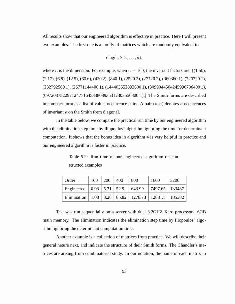
All results show that our engineered algorithm is effective in practice. Here I will present

two examples. The first one is a family of matrices which are randomly equivalent to

diag(1, 2, 3, . . . , n),

wheren is the dimension. For example, whenn = 100, the invariant factors are: [(1 50),

(2 17), (6 8), (12 5), (60 6), (420 2), (840 1), (2520 2), (27720 2), (360360 1), (720720 1),

(232792560 1), (26771144400 1), (144403552893600 1), (3099044504245996706400 1),

(69720375229712477164533808935312303556800 1).] The Smith forms are described

in compact form as a list of value, occurrence pairs. A pair(v, n) denotesn occurrences

of invariantv on the Smith form diagonal.

In the table below, we compare the practical run time by our engineered algorithm

with the elimination step time by Iliopoulos’ algorithm ignoring the time for determinant

computation. It shows that the bonus idea in algorithm 4 is very helpful in practice and

our engineered algorithm is faster in practice.

Table 5.2: Run time of our engineered algorithm on con-

structed examples

Order 100 200 400 800 1600 3200

Engineered 0.93 5.31 52.9 643.99 7497.65 133487

Elimination 1.08 8.28 85.82 1278.73 12881.5 185382

Test was run sequentially on a server with dual 3.2GHZ Xero processors, 6GB

main memory. The elimination indicates the elimination step time by Iliopoulos’ algo-

rithm ignoring the determinant computation time.

Another example is a collection of matrices from practice. We will describe their

general nature next, and indicate the structure of their Smith forms. The Chandler’s ma-

trices are arising from combinatorial study. In our notation, the name of each matrix in

93

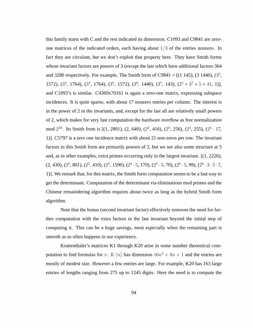
this family starts with C and the rest indicated its dimension. C1093 and C9841 are zero-

one matrices of the indicated orders, each having about1/3 of the entries nonzero. In

fact they are circulant, but we don’t exploit that property here. They have Smith forms

whose invariant factors are powers of 3 (except the last which have additional factors 364

and 3280 respectively. For example, The Smith form of C9841 = [(1 145), (3 1440), (32,

1572), (33, 1764), (34, 1764), (35, 1572), (36, 1440), (37, 143), (24 ∗ 37 ∗ 5 ∗ 41, 1)],

and C1093’s is similar. C4369x70161 is again a zero-one matrix, expressing subspace

incidences. It is quite sparse, with about 17 nonzero entries per column. The interest is

in the power of 2 in the invariants, and, except for the last all are relatively small powers

of 2, which makes for very fast computation the hardware overflow as free normalization

mod232. Its Smith from is [(1, 2801), (2, 640), (22, 416), (23, 256), (24, 255), (24 · 17,

1)]. C5797 is a zero one incidence matrix with about 21 non-zeros per row. The invariant

factors in this Smith form are primarily powers of 2, but we see also some structure at 5

and, as in other examples, extra primes occurring only in the largest invariant. [(1, 2226),

(2, 430), (22, 801), (23, 410), (24, 1590), (24 · 5, 170), (25 · 5, 70), (26 · 5, 99), (26 · 3 · 5 · 7,

1)]. We remark that, for this matrix, the Smith form computation seems to be a fast way to

get the determinant. Computation of the determinant via eliminations mod primes and the

Chinese remaindering algorithm requires about twice as long as the hybrid Smith form

algorithm.

Note that the bonus (second invariant factor) effectively removes the need for fur-

ther computation with the extra factors in the last invariant beyond the initial step of

computing it. This can be a huge savings, most especially when the remaining part is

smooth as so often happens in our experience.

Krattenthaler’s matrices K1 through K20 arise in some number theoretical com-

putation to find formulas forπ. K 〈n〉 has dimension16n2 + 8n + 1 and the entries are

mostly of modest size. However a few entries are large. For example, K20 has 163 large

entries of lengths ranging from 275 up to 1245 digits. Here the need is to compute the

94

determinant (and factor it, which is easy since the factors are smooth). It turns out that

these matrices also have rich structure in their Smith forms, meaning that numerous in-

variant factors are nontrivial and the largest invariant factor is significantly smaller than

the determinant. For this reason, the smooth part of of our Smith form algorithm is the

fastest way we know to compute these determinants.

The practical run time is shown in table 5.3. It turns out that the Chandler’s matri-

ces are favorable by the valence algorithm. In this case, the overhead of our engineered

algorithm is negligible. As shown in the table, our engineer algorithm can yield great

performance in these matrices.

Table 5.3: Run time of our engineered algorithm over prac-

tical examples

name C1093 K 〈10〉 C5797 C9841 C4369x70161

engineered 47.03 7600.83 6445.45 42639.8 67558

Elimination 153.41 13224.2 20807.4 NED NEM

In the table above, NEM stands for “not enough memory”. Test was run sequen-

tially on a server with dual 3.2GHZ Xero processors, 6GB main memory. The elimina-

tion indicates the elimination step time by Iliopoulos’ algorithm ignoring the determinant

computation time.

95

CONCLUSION

In this thesis we have contributed new methods in exact linear algebra for the

computation of minimal polynomial, characteristic polynomial, matrix rank, exact ratio-

nal system solution, and Smith form. Our algorithms improve the state of the art both in

theory (algorithm complexity) and (especially) in practice. Also, We have implemented

all this in the system LinBox and contributed substantially to LinBox in other ways as

well. In future we would like to make further improvements, especially in these areas:

exact solutions of sparse systems and Smith forms of sparse matrices.

96

BIBLIOGRAPHY

[AKS83] M. Ajtai, J. Komlos, and E. Szemeredi. Sorting inc lg(n) parallel steps.Combinatorica, 3:1–19, 1983.

[ASW05] J. Adams, B. D. Saunders, and Z. Wan. Signature of symmetric rationalmatrices and the unitary dual of Lie groups. InProc. of ISSAC’05, 2005.

[Bat68] K.E. Batcher. Sorting networks and their applications. volume 32, pages307–314, 1968.

[BEPP99] H. Bronnimann, I. Z. Emiris, V. Y. Pan, and S. Pion. Sign determination inresidue number systems.Theoret. Comput. Sci., 210:173197, 1999.

[Berar] D. J. Bernstein. Factoring into coprimes in essentially linear time.Journalof Algorithms, to appear.

[BLWW04] Folkmar Bornemann, Dirk Laurie, Stan Wagon, and Jorg Waldvogel. TheSIAM 100-Digit Challenge A Study in High-Accuracy Numerical Comput-ing. SIAM, 2004.

[CC82] T. W. Chou and G. E. Collins. Algorithms for the solution of systems oflinear diophantine equations.Siam J. Comput., 11:687–708, 1982.

[CEK+02] L. Chen, W. Eberly, E. Kaltofen, W. Turner, B. D. Saunders, and G. Villard.Efficient matrix preconditioners for black box linear algebra.LAA 343-344,2002, pages 119–146, 2002.

[CLRS01] T. Cormen, C. Leiserson, R. Rivest, and C. Stein.Introduction to Algorithms,Second edition. MIT Press, 2001.

[Cop95] D. Coppersmith. Solving homegeneous linear equations overGF (2) viablock Wiedemann algorithm.Mathematics of Computation, 62(205):333–350, 1995.

[CS04] Z. Chen and A. Storjohann. An implementation of linear system solving forinteger matrices. InPoster, ISSAC’04, 2004.

97

[CW87] D. Coppersmith and S. Winograd. Matrix multiplication via arithmetic pro-gressions. InProc. 19th ACM STOC, pages 1 – 6, 1987.

[Dem97] J. W. Demmel.Applied Numerical Linear Algebra. SIAM, 1997.

[DGP02] J-G. Dumas, T. Gautier, and C. Pernet. Finite field linear algebra subrou-tines. InProc. ISSAC’02, pages 63 – 74. ACM Press, 2002.

[DGP04] J-G. Dumas, P. Giorgi, and C. Pernet. FFPACK: Finite field linear alge-bra package. InProceedings of the 2004 International Symposium on Sym-bolic and Algebraic Computation, Santander, Spain. ACM Press, New York,2004.

[Dix82] J. D. Dixon. Exact solution of linear equations usingp-adic expansion.Nu-mer. Math., pages 137–141, 1982.

[DPW05] J-G. Dumas, C. Pernet, and Z. Wan. Efficient computation of the character-istic polynomial. InProc. of ISSAC’05, 2005.

[DSV00] J-G. Dumas, B. D. Saunders, and G. Villard. Smith form via the valence:Experience with matrices from homology. InProc. ISSAC’00, pages 95 –105. ACM Press, 2000.

[DSW03] A. Duran, B. D. Saunders, and Z. Wan. Rank of sparse integer matrices. InSiamla 2003, 2003.

[DTW02] J-G. Dumas, W. Turner, and Z. Wan. Exact solution to large sparse integerlinear systems. InPoster, ECCAD 2002, 2002.

[Ebe03] W. Eberly. Early termination over small fields. InProc. ISSAC’03, pages80–87. ACM Press, 2003.

[EGV00] W. Eberly, M. Giesbrecht, and G. Villard. On computing the determinantand Smith form of an integer matrix. InProc. 41st FOCS, pages 675 – 687,2000.

[EK97] W. Eberly and E. Kaltofen. On randomized Lanczos algorithms. InProc.ISSAC’97, pages 176 – 183. ACM Press, 1997.

[Emi98] I. Z. Emiris. A complete implementation for computing general dimensionalconvex hulls.Inter. J. Comput. Geom. Appl., 8:223–253, 1998.

[FH97] X. Fang and G. Havas. On the worst-case complexity of integer guassianelimination. InProc. ISSAC’97, pages 28 –31. ACM Press, 1997.

98

[FM67] G. E. Forsythe and C. B. Moler.Computer Solution of Linear AlgebraicSystems. Prentice-Hall, 1967.

[Fru77] M. A. Frumkin. Polynomial time algorithms in the theory of linear dio-phantine equations. In M. Karpinski, editor,Fundamentals of ComputationTheory, pages 386–392. Springer-Verlag, 1977.

[Gie96] M. Giesbrecht. Probabilistic computation of the Smith normal form of asparse integer matrix. InProc. ANTS’96, pages 173–186. Springer-Verlag,1996.

[Gie01] M. Giesbrecht. Fast computation of the Smith form of a sparse integer ma-trix. Computational Complexity, 10:41–69, 2001.

[GZ02] K.O. Geddes and W.W. Zheng. Exploiting fast hardware floating point inhigh precision computation. Technical report, School of Computer Science,University of Waterloo, CA, December 2002.

[HM91] J. L. Hafner and K. S. McCurley. Asymptotically fast triangularization ofmatrices over rings.Siam J. Comput., 20:1068–1083, 1991.

[Hou64] A. S. Householder.The Theory of Matrices in Numerical Analysis. Blaisdell,Waltham, Mass., 1964.

[Ili89] C. Iliopoulos. Worst-case complexity bounds on algorithms for computingthe canonical structure of finite abelian groups of the Hermite and Smithnormal forms of an integer matrix.SIAM J. Comput., Vol. 18, No.4:658 –669, 1989.

[IMH82] O. Ibarra, S. Moran, and R. Hui. A generalization of the fast LUP matrixdecomposition algorithm and applications.Journal of Algorithms, 3(1):45–56, March 1982.

[Kal95] E. Kaltofen. Analysis of Coppersmith’s block Wiedemann algorithm forthe parallel solution of sparse linear systems.Mathematics of Computation,64(210):777–806, 1995.

[Kal02] E. Kaltofen. An out-sensitive variant of the baby steps / giant steps determi-nant algorithm. InProc. of ISSAC’02, pages 138–144, 2002.

[KB79] R. Kannan and A. Bachem. Polynomial algorithm for computing the Smithand Hermite normal forms of an integer matrix.SIAM J. Comput., Vol 8,No.4:499 – 507, 1979.

99

[KG85] W. Keller-Gehrig. Fast algorithms for the characteristic polynomial.Theo-retical computer science, 36:309–317, 1985.

[KKS90] E. Kaltofen, M. Krishnamoorthy, and B. D. Saunders. Parallel algorithmsfor matrix normal forms.Linear Algebra and its Applications, pages 189 –208, 1990.

[KS91] E. Kaltofen and B. D. Saunders. On Wiedemann’s method of solving sparselinear systems. InProc. AAECC-9, volume 539 ofLect. Notes Comput. Sci.,pages 29–38. Springer Verlag, 1991.

[KV03] E. Kaltofen and G. Villard. On the complexity of computing determinants.Technical Report 36, Laboratoire de l’Informatique du Parallelisme, EcoleNormale Superieure de Lyon, October 2003.

[LSW03] A. Lobo, B. D. Saunders, and Z. Wan. Rank and Smith form of extremelysparse matrices.Abstract. ACA 2003, 2003.

[Mas69] J. L. Massey. Shift-register synthesis and BCH decoding.IEEE Trans. Inf.Theory, 15:122–127, 1969.

[MC79] R. T. Moenck and J. H. Carter. Approximate algorithms to derive exactsolutions to systems of linear equations. InProceedings of the Interna-tional Symposium on Symbolic and Algebraic Computation, pages 65–73.Springer-Verlag, 1979.

[MS04] T. Mulders and A. Storjohann. Certified dense linear system solving.Jounalof symbolic computation, 37(4), 2004.

[New72] M. Newman.Integral Matrices. Academic Press, 1972.

[PW02] V. Pan and X. Wang. Acceleration of Euclidean algorithm and extensions.In Proc. ISSAC’02, pages 207 – 213. ACM Press, 2002.

[PW03] C. Pernet and Z. Wan. Lu based algorithms for the characteristic polynomialover a finite field. InPoster, ISSAC’03. ACM Press, 2003.

[Saa03] Y. Saad.Iterative Methods for Sparse Linear Systems. SIAM, second edi-tion, 2003.

[Sch80] J.T. Schwartz. Fast probabilistic algorithms for verification of polynomialidentities.J. ACM, pages 27:701–717, 1980.

[Smi61] H. M. S. Smith. On systems of indeterminate equations and congruences.Philos. Trans., pages 293–326, 1861.

100

[SSV04] B. D. Saunders, A. Storjohann, and G. Villard. Matrix rank certification.ELECTRONIC Journal of LINEAR ALGEBRA, 11:16–23, 2004.

[Sto96] A. Storjohann. Near optimal algorithms for computing Smith normal formsof integer matrices. InProc. ISSAC’96, pages 267 – 274. ACM Press, 1996.

[Sup03] SuperLU User’s Guide: http://www.nersc.gov/˜xiaoye/SuperLU/ , 2003.

[SW04] B. D. Saunders and Z. Wan. Smith normal form of dense integer matri-ces fast algorithms into practice. InProc. ISSAC’04, pages 274–281. ACMPress, 2004.

[SW05] B. D. Saunders and Z. Wan. Fast early termination technique in symboliclinear algebra. InPoster, ECCAD 2005, 2005.

[TB97] L. N. Trefethen and D. Bau, III.Numerical Linear Algebra. SIAM, 1997.

[Vil00] G. Villard. Computing the frobenius normal form of a sparse matrix. InTheThird International Workshop on Computer Algebra in Scientific Computing,pages 395–407, Oct, 2000.

[vzGG99] J. von zur Gathen and J. Gerhard.Modern Computer Algebra. CambridgeUniversity Press, 1999.

[Wan04] Z. Wan. An algorithm to solve integer linear systems exactly using numericalmethods.Journal of Symbolic Computation, submitted, 2004.

[Wie86] D. Wiedemann. Solving sparse linear equations over finite fields.IEEETrans. Inform. Theory, 32:54 – 62, 1986.

101