computing the greatest common divisor of multivariate
TRANSCRIPT
Computing the Greatest Common Divisor of
Multivariate Polynomials over Finite Fields
Suling Yang
Simon Fraser University
Abstract
Richard Zippel’s sparse modular GCD algorithm is widely used tocompute the monic greatest common divisor (GCD) of two multivariatepolynomials over Z. In this report, we present how this algorithm canbe modified to solve the GCD problem for polynomials over finite fieldsof small cardinality. When the GCD is not monic, Zippel’s algorithmcannot be applied unless the normalization problem is resolved. In [6],Alan Wittkopf et al. developed the LINZIP algorithm for solving thenormalization problem. Mahdi Javadi proposed a refinement to theLINZIP algorithm in [4]. We implemented his approach and will showthat it is efficient and effective on polynomials over small finite fields.Zippel’s algorithm also uses properties of transposed Vandermonde sys-tems to reduce the time and space complexity of his algorithm. Wealso investigated how this can be applied to our case.
1 Introduction
Let A and B be polynomials in F [x1, . . . , xn], where F is a unique factoriza-tion domain (UFD) and n is a positive integer. Our goal is to find a greatestcommon divisor (GCD) G of A and B. Let A = A/G, B = B/G be thecofactors of A and B, respectively. When n = 1, A and B are univariate,and so is G. In this case the Euclidean algorithm can be used. However,we want to develop efficient algorithms for computing multivariate GCD,
1

1 INTRODUCTION 2
because the size of coefficients grows rapidly in F [x1, . . . , xn] when usingthe primitive Euclidean algorithm [2]. This problem is similar to the growthin the size of coefficients when using naive methods to solve linear equa-tions over F [x1, . . . , xn]. Using homomorphisms to map the GCD problemto a simpler domain can improve arithmetic calculation and lead to betterapproaches to avoid the problems with coefficient growth.
In [1], Brown developed a modular algorithm which consists of two pro-cedures to find the GCD of A and B when A and B are polynomials with in-teger coefficients Z. Brown’s algorithm finds the GCD’s images in univariatedomain, and then uses Chinese Remainder Theorem (CRT) or PolynomialInterpolation to get the original GCD. The running time of Brown’s algo-rithm depends on the total degree of G. In [5] Erich Kaltofen and MichaelMonagan explored the generic setting of the modular GCD algorithm. Theyshowed how it could be applied to GCD problem over the Euclidean ringZ/(p)[t], where Z/(p) denotes the integer residues modulo p. They also com-pared it with other algorithms in the domain Z/(p)[t][x] and established itas better than the known other standard methods.
Zippel presented a sparse modular algorithm which improved the com-plexity of Brown’s algorithm for sparse G, by reducing the number of uni-variate images required in [7]. Zippel’s algorithm obtains an assumed formof G by recursively applying the algorithm in one fewer variable, and thencalculates the constant coefficients from univariate GCD images (we call thisSparse Interpolation). It is a Las Vegas algorithm which always results in acorrect solution or declares failure. Sparse interpolation requires nmax + 1images where nmax is the maximum number of terms of the coefficients ofthe main variable x1 in G. In [8] Zippel analyzed the properties of Van-dermonde matrices, whose entries are powers of a same constant in eachcolumn and same power in each row. Zippel constructed an algorithm tofind the inverse of a Vandermonde matrix using linear space and quadratictime. We call it LinSpaceSol algorithm. We will discuss these properties ofVandermonde matrices in the next section.
If the GCD G is non-monic in the main variable x1, for example, G =(x5
2 +x3)x81 +(x2 +x3)x2
1 +(x2 +x23 +1) ∈ Z[x2, x3][x1], then Zippel’s sparse

2 RELATED WORK 3
modular algorithm cannot be applied directly. This is called the normaliza-tion problem. In order to solve this problem efficiently, de Kleine, Monaganand Wittkopf implemented the LINZIP algorithm which uses O(n3
1 + n32 +
· · ·+n3t ) time, where t is the number of terms in G when it is written in the
collected form in the main variable x1, and ni’s are the numbers of termsin the coefficients of x1. E.g. for the above example, t = 3, n1 = 2, n2 = 2,and n3 = 3. In [4], M. Javadi developed a more efficient method to solvethe normalization problem using only O((n1 + · · ·+ nk)3 + n2
k+1 + · · ·+ n2t )
time, where n1 ≤ n2 ≤ · · · ≤ nt and k is the number of coefficients of x1
that the algorithm needs to compute the scaling factor.In the following section, we discuss the work from previous authors.
Then, the algorithms of solving the GCD problems over finite fields of smallcardinalities are given in Section 3. In Section 4, we analyze the probabilityof getting an incorrect result, and thus triggering a restart. Experimentalresults of the effectiveness and efficiency are given in Section 5. Section 6concludes this report by providing some potential improvement.
2 Related Work
2.1 Modular GCD Algorithm
Consider A,B ∈ Z[x1, · · · , xn]. Brown’s algorithm for solving the GCDproblem in Z[x1, · · · , xn] consists two algorithms, MGCD and PGCD, to dealwith different types of homomorphisms in Z[x1, · · · , xn]. The MGCD algo-rithm reduces a GCD problem to a series of GCD problems in Zpi [x1, · · · , xn]by applying modular homomorphisms [1]. It chooses a sequence of primespi ∈ Z, such that pi does not divide LCX(A), LCX(B) where LCX(A) meansthe leading coefficient of A in the lexicographic order of X = [x1, · · · , xn],and repeatedly calls PGCD to obtain Gi = gcd(A mod pi, B mod pi). Itapplies the Chinese Remainder Theorem (CRT) on all Gi’s with moduli pi’sincrementally and the stabilized image is G if it divides both A and B.
Similarly, the PGCD algorithm reduces the Zpi [x1, · · · , xn] GCD prob-lem to a series of (n−2)-variate finite field GCD problems in Zpi [x1, · · · , xn−1]

2 RELATED WORK 4
by applying evaluation homomorphisms. It chooses αj ∈ Zpi such thatLCX(A)(xn−1 = αj), LCX(B)(xn−1 = αj) 6= 0 where X = [x1, · · · , xn−1].Then it recursively calls itself to obtain Gi,j = gcd((A mod pi)(xn−1 =αj), (B mod pi)(xn−1 = αj)). Then, it applies polynomial interpolation oncoefficients of Gi,j to interpolate xn−1 incrementally stopping when the inter-polated result stabilizes, and the stabilized image is Gi = gcd(A mod pi, B
mod pi) if it divides both A mod pi and B mod pi in Zpi [x1, · · · , xn].
2.2 Problems with the Modular GCD Algorithm
After the major problem is reduced to a simpler problem over a more al-gebraic structure domain which allows for a wider range of algorithms, thearithmetic is simpler because the arithmetic is done in a domain with smallcoefficients. However, the trade-off is information loss, which may result infailure in some cases. Let G = gcd(A,B) where A,B ∈ Z[x1, · · · , xn], andlet A = A/G, B = B/G. Let H = gcd(φp(A), φp(B)) in Zp[x1, · · · , xn]. Theproblem is that H may not be a scalar multiple of φp(G).
Definition 2.1. A homomorphism φ is bad if degx1(φ(G)) < degx1
(G). Ifdegx1
(φ(G)) = degx1(G mod p) < degx1
(G) where p is a prime in Z, thenp is bad. Similarly, if degx1
(φ(G)) = degx1(G mod I) < degx1
(G) whereI = < x2 − α2, ..., xn − αn >,αi ∈ Zp, then the evaluation point (α2, ..., αn)is bad.
Definition 2.2. A homomorphism φ is unlucky if
degx1(GCD(φ(A), φ(B))) > 0.
Bad homomorphisms can be prevented if we choose p and (α2, ..., αn)such that LCx1(A) mod p 6= 0 and LCx1(B) mod I 6= 0. However, unluckyhomomorphisms cannot be detected in advance. Instead, by the applicationof the following lemma, Brown’s algorithms can identify unlucky homomor-phisms at execution time.

2 RELATED WORK 5
Lemma 2.3. (Lemma 7.3 from Geddes et al. [2]) Let R and R′ be UFD’swith φ : R → R′ a homomorphism of rings. This induces a natural homo-morphism, also denoted by φ, from R[x] to R′[x]. Suppose A(x), B(x) ∈ R[x]and G(x) = GCD(A(x), B(x)) with φ(LC(G(x))) 6= 0. Then
degx(GCD(φ(A(x)), φ(B(x)))) ≥ degx(GCD(A(x), B(x))). (2.1)
Therefore, we can eliminate a univariate image of higher degree than otherunivariate images. The probability of getting an unlucky evaluation pointis analyzed in Section 4.Example 1:
A = (x + y + 11)(3x + y + 1)
B = (x + y + 4)(3x + y + 1)
If we choose p = 3, then gcd(A mod 3, B mod 3) = y + 1, which hasdegree 0 in x. Thus, p = 3 is bad. If we choose p = 7, then gcd(A mod 3, B
mod 3) = (x + y + 4)(3x + y + 1). Thus, p = 7 is unlucky.
2.3 Sparse Modular GCD Algorithm
We have seen in the previous sections that modular GCD algorithms cansolve problems by reducing a complex problem into a number of easier prob-lems. However, another problem that arises from this approach is the growthin the number of univariate GCD images required. In many cases, especiallywhen polynomials are multivariate, G is sparse, i.e., the number of nonzeroterms is generally much smaller than the number of possible terms up toa given total degree d. Hence, sparse algorithms may be more efficient.Zippel introduced a sparse algorithm for calculating the GCD of two mul-tivariate polynomials over the integer [7]. We will show the pseudo-code ofthe algorithm applied on finite fields in the next section. This approach isprobabilistic, and we will estimate the likelihood of success in the Section 4.
One observation is that if an evaluation point is chosen at random froma large enough set, then evaluating a polynomial at that point is rarely zero.

2 RELATED WORK 6
Based on this observation, the sparse modular methods determine a solutionfor one small domain by normal approach, and then use sparse interpolationsto find solutions for other small domains. For a GCD problem in n variableswhere the actual GCD has total degree d, a dense interpolation, for instance,Newton interpolation, requires (d + 1)n evaluation points, since it assumesnone of the possible terms is absent. Sparse interpolation assumes thatthe image Gf from the dense interpolation is of correct form, and it is todetermine t coefficients where t is the number of terms in Gf and t � d.Hence, it requires only O (n(t + 1)(d + 1)) evaluation points.
2.4 Vandermonde Matrices Applied to Interpolation
In the sparse interpolation, we need to find solutions for a set of linear equa-tions over a field F , i.e., we need to find the inverse of the matrix formed bythese equations. Algorithms for finding inverses of general matrices requireO(n3) arithmetic operations in F and space for O(n2) elements of F , wheren is the number of rows/columns. But for Vandermonde matrices, one canfind the inverse using O(n) space and O(n2) arithmetic operations. Theform of a Vandermonde matrix is as follows.
Vn =
1 k1 k2
1 . . . kn−11
1 k2 k22 . . . kn−1
2...
...... . . .
...1 kn k2
n . . . kn−1n
, (2.2)
where the ki are chosen from F . We can easily calculate the determinantof a Vandermonde matrix. We can observe that multiplying the ith columnby k1 and subtract it from the i + 1th column we get,
det Vn =
∣∣∣∣∣∣∣∣∣∣1 0 0 . . . 01 k2 − k1 k2
2 − k1k2 . . . kn−12 − k1k
n−22
......
... . . ....
1 kn − k1 k2n − k1kn . . . kn−1
n − k1kn−2n
∣∣∣∣∣∣∣∣∣∣.
2 RELATED WORK 7
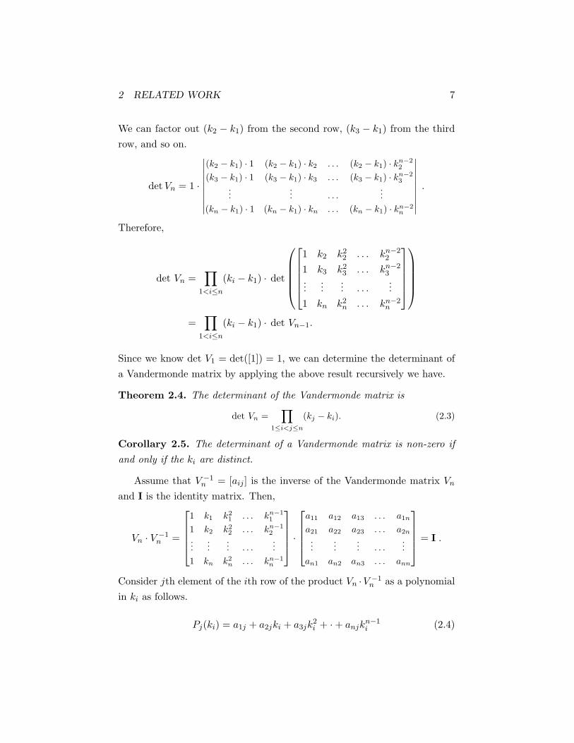
We can factor out (k2 − k1) from the second row, (k3 − k1) from the thirdrow, and so on.
det Vn = 1 ·
∣∣∣∣∣∣∣∣∣(k2 − k1) · 1 (k2 − k1) · k2 . . . (k2 − k1) · kn−2
2
(k3 − k1) · 1 (k3 − k1) · k3 . . . (k3 − k1) · kn−23
...... . . .
...(kn − k1) · 1 (kn − k1) · kn . . . (kn − k1) · kn−2
n
∣∣∣∣∣∣∣∣∣ .
Therefore,
det Vn =∏
1<i≤n
(ki − k1) · det
1 k2 k22 . . . kn−2
2
1 k3 k23 . . . kn−2
3...
...... . . .
...1 kn k2
n . . . kn−2n
=∏
1<i≤n
(ki − k1) · det Vn−1.
Since we know det V1 = det([1]) = 1, we can determine the determinant ofa Vandermonde matrix by applying the above result recursively we have.
Theorem 2.4. The determinant of the Vandermonde matrix is
det Vn =∏
1≤i<j≤n
(kj − ki). (2.3)
Corollary 2.5. The determinant of a Vandermonde matrix is non-zero ifand only if the ki are distinct.
Assume that V −1n = [aij ] is the inverse of the Vandermonde matrix Vn
and I is the identity matrix. Then,
Vn · V −1n =
1 k1 k2
1 . . . kn−11
1 k2 k22 . . . kn−1
2
......
... . . ....
1 kn k2n . . . kn−1
n
·
a11 a12 a13 . . . a1n
a21 a22 a23 . . . a2n
......
... . . ....
an1 an2 an3 . . . ann
= I .
Consider jth element of the ith row of the product Vn ·V −1n as a polynomial
in ki as follows.
Pj(ki) = a1j + a2jki + a3jk2i + ·+ anjk
n−1i (2.4)

2 RELATED WORK 8
Then we know,
Pj(ki) =
1 if i = j
0 otherwise(2.5)
By choosing the Pj(Z) to be
Pj(Z) =∏l 6=j
1≤l≤n
Z − kl
kj − kl,
we can verify that equation (2.5) holds, and thus the coefficients of the Pj
are the columns of V −1n . Let P (Z) =
∏1≤l≤n(Z − kl), the master polyno-
mial, which can be computed in O(n2) multiplications. Then we calculatePj(Z) =
∏l 6=j
1≤l≤n(Z − kl) = P (Z)/(Z − kj). Thus Pj(Z) can be computed
using polynomial division, and then Pj(Z) = Pj(Z)/Pj(kj) can be computedusing scalar division. This requires only O(n) space and time. We want tocalculate X = (X1, · · · , Xn) such that,
X1 + k1X2 + k21X3 + · · ·+ kn−1
1 Xn = w1
X1 + k2X2 + k22X3 + · · ·+ kn−1
2 Xn = w2
... =...
Xn + knX2 + k2nX3 + · · ·+ kn−1
n Xn = wn
⇔ Vn · XT =
w1
w2
...wn
.
Then, XT = V −1n · (w1, · · · , wn)T and we get
X1
...Xn
=
w1 · coef(P1, Z
0)...
w1 · coef(P1, Zn−1)
+ · · ·+
wn · coef(Pn, Z0)
...wn · coef(Pn, Zn−1)
. (2.6)
Since the inverse of the transpose of a matrix is the transpose of the inverse,this approach can also be applied to a transposed Vandermonde matrix,

2 RELATED WORK 9
which has the following form.
1 1 · · · 1k1 k2 · · · kn
k21 k2
2 · · · k2n
......
......
kn−11 kn−1
2 · · · kn−1n
(2.7)
Then, for V Tn · X = (w1, · · · , wn)T , we get X = (V T
n )−1 · (w1, · · · , wn)T =(V −1
n )T · (w1, · · · , wn)T , and thusX1
...Xn
=
w1 · coef(P1, Z
0)...
w1 · coef(Pn, Z0)
+ · · ·+
wn · coef(P1, Z
n−1)...
wn · coef(Pn, Zn−1)
. (2.8)
We can use this technique to determine G = gcd(A,B) = c1Xe1 +· · ·+ctX
et ,where X = [x1, · · · , xn] and ei is a vector representing the degrees. First,we choose a random n-tuple α = (α1, · · · , αn). Second, evaluate G(α) =c1α
e1 + · · · + ctαet and denote the value of each monomial X ei by mi, so
that G(α) = c1m1+ · · ·+ctmt. Third, we observe that (αj)ei = (αei)j = mji .
Thus we have the following system of equations in the form of a transposedVandermonde system.
G(α0) = c1 + c2 + · · ·+ ct
G(α1) = c1m1 + c2m2 + · · ·+ ctmt
G(α2) = c1m21 + c2m
22 + · · ·+ ctm
2t
......
G(αt−1) = c1mt−11 + c2m
t−12 + · · ·+ ctm
t−1t .
We check if all mi’s are distinct. If they are, the above system has a uniquesolution and can be solved in O(t2) time and O(t) space by calculatingthe master polynomial P (Z) and each Pj(Z), and then using (2.8). Thistechnique is also used in M. Javadi’s algorithm for solving non-monic GCDproblems.
2 RELATED WORK 10
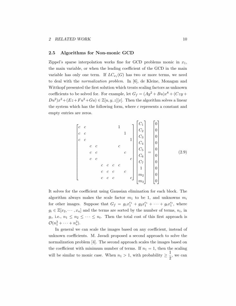
2.5 Algorithms for Non-monic GCD
Zippel’s sparse interpolation works fine for GCD problems monic in x1,the main variable, or when the leading coefficient of the GCD in the mainvariable has only one term. If LCx1(G) has two or more terms, we needto deal with the normalization problem. In [6], de Kleine, Monagan andWittkopf presented the first solution which treats scaling factors as unknowncoefficients to be solved for. For example, let Gf = (Ay2 + Bu)x8 + (Czy +Du2)x2+(Ez+Fu2+Gu) ∈ Z[u, y, z][x]. Then the algorithm solves a linearthe system which has the following form, where c represents a constant andempty entries are zeros.
c c 1c c 1c c 1
c c c
c c c
c c c
c c c c
c c c c
c c c c
C1
C2
C3
C4
C5
C6
C7
1m2
m3
=
0000000000
(2.9)
It solves for the coefficient using Gaussian elimination for each block. Thealgorithm always makes the scale factor m1 to be 1, and unknowns mi
for other images. Suppose that Gf = g1xe11 + g2x
e11 + · · · + gtx
et1 , where
gi ∈ Z[x2, · · · , xn] and the terms are sorted by the number of terms, ni, ingi, i.e., n1 ≤ n2 ≤ · · · ≤ nt. Then the total cost of this first approach isO(n3
1 + · · ·+ n3s).
In general we can scale the images based on any coefficient, instead ofunknown coefficients. M. Javadi proposed a second approach to solve thenormalization problem [4]. The second approach scales the images based onthe coefficient with minimum number of terms. If n1 = 1, then the scaling
will be similar to monic case. When n1 > 1, with probability ≥ 12, we can
3 THE ALGORITHM 11
find the leading coefficient by solving only a system of size n1 +n2−1 terms.After finding the leading coefficient using O((n1 + n2)3) time, we can useZippel’s linear space and quadratic time algorithm to find other constantcoefficients using O(n2
i ) time. However, there may be a common factoramong g1 and g2. Say G = (y2+uy)x8+(uy+u2)x2+(z+u2+u), which hasassumed form Gf = (Ay2+Buy)x8+(Czy+Du2)x2+(Ez+Fu2+Gu). Thengcd(g1, g2) = gcd(y2 +uy, uy+u2) = (y+u). Then the system to solve A, B,C, and D has no solution no matter how many evaluation points we choose.Therefore, we have to solve for a same system as in (2.9) usingO(n3
1+· · ·+n3s)
time. Suppose that we need k coefficients of x1 to form a system with nounlucky factor. We know k < t, because contx1A = contx1B = 1. ThenJavadi’s approach requires O((n1 + · · ·+ nk)3 + n2
k+1 + · · ·+ n2t ) time.
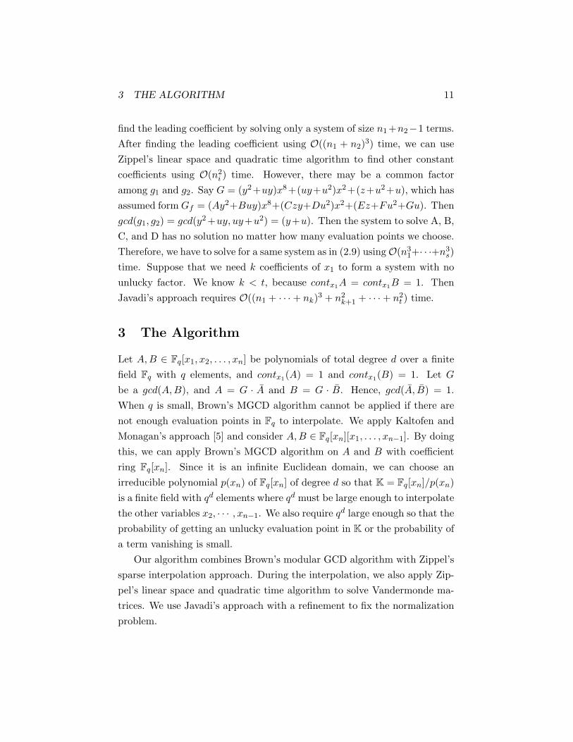
3 The Algorithm
Let A,B ∈ Fq[x1, x2, . . . , xn] be polynomials of total degree d over a finitefield Fq with q elements, and contx1(A) = 1 and contx1(B) = 1. Let G
be a gcd(A,B), and A = G · A and B = G · B. Hence, gcd(A, B) = 1.When q is small, Brown’s MGCD algorithm cannot be applied if there arenot enough evaluation points in Fq to interpolate. We apply Kaltofen andMonagan’s approach [5] and consider A,B ∈ Fq[xn][x1, . . . , xn−1]. By doingthis, we can apply Brown’s MGCD algorithm on A and B with coefficientring Fq[xn]. Since it is an infinite Euclidean domain, we can choose anirreducible polynomial p(xn) of Fq[xn] of degree d so that K = Fq[xn]/p(xn)is a finite field with qd elements where qd must be large enough to interpolatethe other variables x2, · · · , xn−1. We also require qd large enough so that theprobability of getting an unlucky evaluation point in K or the probability ofa term vanishing is small.
Our algorithm combines Brown’s modular GCD algorithm with Zippel’ssparse interpolation approach. During the interpolation, we also apply Zip-pel’s linear space and quadratic time algorithm to solve Vandermonde ma-trices. We use Javadi’s approach with a refinement to fix the normalizationproblem.

3 THE ALGORITHM 12
3.1 MGCD Algorithm Applied on Finite Field
In the MGCD algorithm of Brown’s modular algorithm, we could choosedegxn
p > degxnG in which case one irreducible polynomial p ∈ Z[xn]
would be sufficient. However, it is more efficient to apply the Chinese Re-mainder Theorem (CRT) and choose several pi(xn) such that
∑degxn
pi >
degxnG and |Ki| is just big enough for evaluation and interpolation, where
Ki = Fq[xn]/pi(xn). To avoid the bad “prime” problem, we also need tochoose pi ∈ Fq[xn] such that pi does not divide LCX(A) and LCX(B)where X = [x1, · · · , xn−1]. Then, algorithm PGCD is called repeatly to getGi = gcd(A/pi, B/pi). The homomorphism φpi : Fq[xn][x1, · · · , xn−1] →Ki[x1, · · · , xn−1] restricts the polynomial coefficients to be of lower degreethan pi, and hence stops the growth in the coefficients. Then, we can obtainG by applying the CRT on Gi’s with moduli pi’s. We will use Ki to denotethe finite field Fq[xn]/pi. The algorithm is shown in Figure 1.
3.2 PGCD Algorithm Applied on Finite Field
Similarly, PGCD uses the evaluation homomorphism to reduce the GCDproblem for A,B ∈ Ki[x1, · · · , xn−1] to a series of problems in Ki[x1, · · · , xn−2],i.e., it reduces (n − 1)-variate problem to a series of (n − 2)-variate prob-lems. Let αj ∈ Ki such that xn−1 − αj does not divide LCX(A) norLCX(B) where X = [x1, · · · , xn−2]. The evaluation homomorphism φαj :Ki[x1, . . . , xn−1]→ Ki[x1, . . . , xn−2] maps A(x1, · · · , xn−1) to A(x1, ..., xn−2, αj)= Aij and B(x1, · · · , xn−1) to B(x1, ..., xn−2, αj) = Bij . PGCD calls it-self recursively and finally reduces the problem to univariate GCD prob-lems which can be solved using Euclidean algorithm (EA). To obtain Gi =gcd(A, B), PGCD chooses several αj ’s and obtains Gij = gcd(Aij , Bij) byrecursively calling itself. Then it interpolates the Gij ’s and αj ’s. The algo-rithm is shown in Figure 2.
3.3 Sparse Interpolation Applied on Finite Field
When G is sparse, dense interpolation is not efficient. For example, if MGCDchooses irreducible polynomials of degree 5 in F2[z] for G = x10 +(y10 +z5 +
3 THE ALGORITHM 13
2z + 1)x2 + z14 mod 2, then it requires three of them polynomials and 11evaluation values for each of them. Thus, it requires 33 univariate images intotal. On the other hand, after we calculate the univariate images using oneirreducible polynomial, we obtain the assumed form Gf = x10 + (C1y
10 +C2)x2+C3 from a dense interpolation of y. Then we just need two univariateimages for each of the other two irreducible polynomials.Example 2:Let G1 = x10+W11x
2+W12 and G2 = x10+W21x2+W22 be the images when
y = α1 and y = α2 respectively. Then we can set up two linear systems,[α10
1 1α10
2 1
]·
[C1
C2
]=
[W11
W21
]and
[C3
C3
]=
[W12
W22
], (3.1)
and solve for C1, C2, and C3. Then, it requires only 11 (for the dense in-terpolation) +4 (for two sparse interpolations) = 15 univariate images intotal. However, if we choose p1(z) = z5 + z + 1, then the coefficient of x2 isjust C1y
10. Then constant term C2 is absent in the assumed form, and thusthe first system in 3.1 becomes[
α101
α102
]·
[C3
C3
]=
[W11
W21
]
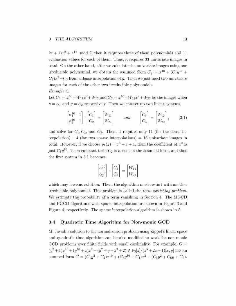
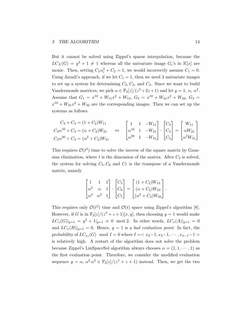
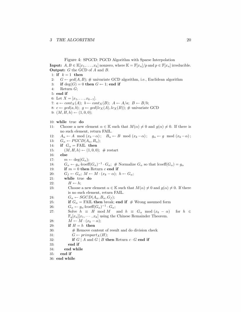
which may have no solution. Then, the algorithm must restart with anotherirreducible polynomial. This problem is called the term vanishing problem.We estimate the probability of a term vanishing in Section 4. The MGCDand PGCD algorithms with sparse interpolation are shown in Figure 3 andFigure 4, respectively. The sparse interpolation algorithm is shown in 5.
3.4 Quadratic Time Algorithm for Non-monic GCD
M. Javadi’s solution to the normalization problem using Zippel’s linear spaceand quadratic time algorithm can be also modified to work for non-monicGCD problems over finite fields with small cardinality. For example, G =(y2 +1)x10 +(y10 + z)x2 +(y2 +y + z3 +2) ∈ F3[z]/(z5 +2z +1)[x, y] has anassumed form G = (C1y
2 + C2)x10 + (C3y10 + C4)x2 + (C5y
2 + C6y + C7).
3 THE ALGORITHM 14
But it cannot be solved using Zippel’s sparse interpolation, because theLCX(G) = y2 + 1 6= 1 whereas all the univariate image Gi’s in K[x] aremonic. Then, setting C1α
2i + C2 = 1, we would incorrectly assume C1 = 0.
Using Javadi’s approach, if we let C1 = 1, then we need 3 univariate imagesto set up a system for determining C2, C3, and C4. Since we want to buildVandermonde matrices, we pick α ∈ F3[z]/(z5 +2z+1) and let y = 1, α, α2.Assume that G1 = x10 + W11x
2 + W12, G2 = x10 + W21x2 + W22, G3 =
x10 + W31x2 + W32 are the corresponding images. Then we can set up the
systems as follows.
C3 + C4 = (1 + C2)W11
C3α10 + C4 = (α + C2)W21
C3α20 + C4 = (α2 + C2)W31
⇔
1 1 −W11
α10 1 −W21
α20 1 −W31
·C3
C4
C2
=
W11
αW21
α2W31
This requires O(t3) time to solve the inverse of the square matrix by Gaus-sian elimination, where t is the dimension of the matrix. After C2 is solved,the system for solving C5, C6 and C7 is the transpose of a Vandermondematrix, namely 1 1 1
α2 α 1α4 α2 1
·C5
C6
C7
=
(1 + C2)W13
(α + C2)W23
(α2 + C2)W33
.
This requires only O(t2) time and O(t) space using Zippel’s algorithm [8].However, if G is in F2[z]/(z5 + z + 1)[x, y], then choosing y = 1 would makeLCx(G)|y=1 = y2 + 1|y=1 ≡ 0 mod 2. In other words, LCx(A)|y=1 = 0and LCx(B)|y=1 = 0. Hence, y = 1 is a bad evaluation point. In fact, theprobability of LCx1(G) mod I = 0 where I =< x2−1, x3−1, · · · , xn−1−1 >
is relatively high. A restart of the algorithm does not solve the problembecause Zippel’s LinSpaceSol algorithm always chooses α = (1, 1, · · · , 1) asthe first evaluation point. Therefore, we consider the modified evaluationsequence y = α, α2 α3 ∈ F2[z]/(z5 + z + 1) instead. Then, we get the two

3 THE ALGORITHM 15
systems as follows.α10 1 −W11
α20 1 −W21
α30 1 −W31
·C3
C4
C2
=
αW11
α2W21
α3W31
,
α2 α 1α4 α2 1α6 α3 1
·C5
C6
C7
=
(α + C2)W13
(α2 + C2)W23
(α3 + C2)W33
.
Again this requires O(t3) time to solve the first system, where t is thedimension of the first square matrix. The second system involves solving theinverse of a transpose of a generalized Vandermonde matrix. We consider ageneral Vandermonde matrix Vt and its inverse V −1
t as follows.
Vt · V −1t =
k1 k2
1 k31 . . . kt
1
k2 k22 k3
2 . . . kt2
......
... . . ....
kt k2t k3
t . . . ktt
·
a11 a12 a13 . . . a1t
a21 a22 a23 . . . a2t
......
... . . ....
at1 at2 at3 . . . att
= I.
Consider jth element of the ith row of the product Vt ·V −1t as a polynomial,
Pj(ki) = a1jki + a2jk2i + a3jk
3i + · + anjk
ti . Using the similar technique in
Section 2, we can let
Pj(Z) =Z
kj
∏l 6=j
1≤l≤t
Z − kl
kj − kl. (3.2)
We can easily verify that Pj(kj) = 1 and Pj(ki) = 0 ∀i 6= j. The masterpolynomial for this case is P (Z) = Z ·
∏1≤l≤t(Z − kl). Then we calculate
Pj(Z) = Z ·∏
l 6=j1≤l≤t
(Z−kl) = P (Z)/(Z − kj). Thus Pj(Z) can be computed
using polynomial division, and then Pj(Z) =Pj(Z)Pj(kj)
can be computed using
scalar division. Again, this requires only O(t) space and time to computeeach Pj . Then, we can find V −1
t by calculating all Pj ’s, 1 ≤ j ≤ t, andthen obtaining the coefficients. To solve Vt · CT = (w1, · · · , wt)T whereC = (C1, · · · , Ct), we can calculate
Cj = w1 · coef(P1, Zj) + · · ·+ wt · coef(Pt, Z
j). (3.3)

3 THE ALGORITHM 16
Since the inverse of the transpose of a matrix is the transpose of the inverse,we can calculate V T
t ·CT = (w1, · · · , wt)T using the same master polynomialand Pj(Z)’s. We have
Cj = w1 · coef(Pj , Z1) + · · ·+ wt · coef(Pj , Z
t). (3.4)
As in Section 2, we write G = gcd(A,B) = c1Xe1 + · · · + ctX
et , whereX = [x1, · · · , xn] and ei is a degree vector. First, we choose a random n-tuple α = (α1, · · · , αn) ∈ Kn. Second, evaluate G(α) = c1α
e1 + · · · + ctαet
and denote the value of each monomial by mi, i.e., G(α) = c1m1+· · ·+ctmt.Third, we observe that (αj)ei = (αei)j = mj
i . Thus we have the followingsystem of equations in the form of a transposed Vandermonde system.
G(α1) = c1m1 + c2m2 + · · ·+ ctmt
G(α2) = c1m21 + c2m
22 + · · ·+ ctm
2t
......
G(αt) = c1mt1 + c2m
t2 + · · ·+ ctm
tt .
This system can be solved in O(t2) time and O(t) space by calculating themaster polynomial P (Z) and each Pj(Z), and then calculating each Ci usingequation (3.4). This refinement of sparse interpolation is shown in Figure 6.

3 THE ALGORITHM 17
Figure 1: MGCD: Brown’s Modular GCD AlgorithmInput: A,B ∈ Fq[xn][x1, . . . , xn−1], nonzero.Output: G the GCD of A and B.1: if n = 1 then2: G← gcd(A,B); # Call univariate GCD algorithm, i.e., Euclidean algorithm3: if deg(G) = 0 then G← 1; end if4: Return G;5: end if6: Let X = [x1, . . . , xn−1].7: a← contX(A); b← contX(B); A← A/a; B ← B/b; # Remove scalar content8: c← gcd(a, b); g ← gcd(lcX(A), lcX(B)); # univariate GCD9: (M,H, h)← (1, 0, 0); l← min(degx1
(A),degx1(B));
10: d← min(degX(A),degX(B)); s← dlogq(2 d2)e;
11: while true do12: Choose an irreducible polynomial p ∈ Fq[xn] such that p - M , p - g and
degxn(p) ≥ s.
13: Ap ← A mod p ; Bp ← B mod p ; # Ap, Bp ∈ Fqs [x1, . . . , xn−1]14: gp ← g mod p ; # univariate GCD15: Gp ← PGCD(Ap, Bp) ∈ Fqs [x1, . . . , xn−1]∪ FAIL ;16: if Gp = FAIL then17: (M,H, h)← (1, 0, 0); l← min(degx1
(A),degx1(B)); # restart
18: else19: m← degx1
(Gp);20: Gp ← gp·lcoeff(Gp)−1 ·Gp; # Normalize Gp so that lcoeff(Gp) = gp
21: if m = 0 then22: Return c;23: else if m < l then24: l← m; M ← p; h← Gp
25: else if m = l then26: H ← h;27: Solve h ≡ H mod M and h ≡ Gp mod p for h ∈ Fq[xn][x1, · · · , xn]
using Chinese Remainder Theorem.28: M ←M · p29: end if30: if H = h then31: # Remove content of result and do division check32: G← primpartX(H);33: if G | A and G | B then Return c ·G end if34: end if35: end if36: end while

3 THE ALGORITHM 18
Figure 2: PGCD: Multivariate GCD Reduction AlgorithmInput: A,B ∈ K[x1, . . . , xk] nonzero, where K = F[xn]/p and p ∈ F[xn] irreducible.Output: G the GCD of A and B.1: if k = 1 then2: G← gcd(A,B); # univariate GCD algorithm, i.e., Euclidean algorithm3: if deg(G) = 0 then G← 1; end if4: Return G;5: end if6: Let X = [x1, . . . , xk−1].7: a← contX(A); b← contX(B); A← A/a; B ← B/b;8: c← gcd(a, b); g ← gcd(lcX(A), lcX(B)); # univariate GCD9: (M,H, h)← (1, 0, 0); l← min(degx1
(A),degx1(B));
10: while true do11: Choose a new element α ∈ K such that M(α) 6= 0 and g(α) 6= 0. If there is no
such element, then return FAIL. # The coefficient ring is not large enough.12: Aα ← A mod (xk−α) ; Bα ← B mod (xk−α) ; gα ← g mod (xk−α) ;13: Gα ← PGCD(Aα, Bα) ∈ Fqs [x1, . . . , xk−1]∪ FAIL ;14: if Gα = FAIL then15: (M,H, h)← (1, 0, 0); l← min(degx1
(A),degx1(B)); # restart
16: else17: m← degx1
(Gα);18: Gα ← gα·lcoeff(Gα)−1 ·Gα; # Normalize Gα so that lcoeff(Gα) = gα
19: if h = 0 or m < l then20: l← m; H ← h; h← Gα; M ← (xk − α);21: else if m = l then22: H ← h;23: Solve h ≡ H mod M and h ≡ Gα mod (xk − α) for h ∈
Fq[xn][x1, · · · , xk] using the Chinese Remainder Theorem.24: M ←M · p25: end if26: if H = h then27: # Remove content of result and do division check28: G← primpartX(H);29: if G | A and G | B then Return c ·G end if30: end if31: end if32: end while

3 THE ALGORITHM 19
Figure 3: SMGCD: MGCD Algorithm with Sparse InterpolationInput: A,B ∈ Fq[xn][x1, . . . , xn−1], nonzero.Output: G the GCD of A and B1: if n = 1 then2: G← gcd(A,B); # Call univariate GCD algorithm, i.e., Euclidean algorithm3: if deg(G) = 0 then G← 1; end if4: Return G;5: end if6: Let X = [x1, . . . , xn−1].7: a← contX(A); b← contX(B); A← A/a; B ← B/b; # Remove scalar content8: c← gcd(a, b); g ← gcd(lcX(A), lcX(B)); # univariate GCD9: (M,H, h)← (1, 0, 0);
10: d← min(degX(A),degX(B)); s← dlogq(2 d2)e
11: while true do12: Choose a new irreducible polynomial p ∈ F[xn] such that p - M , p - g and
degxn(p) ≥ s.
13: Ap ← A mod p ; Bp ← B mod p ; gp ← g mod p ;14: Gp ← PGCD(Ap, Bp);15: if Gp = FAIL then16: (M,H, h)← (1, 0, 0); # restart17: else18: m← deg(Gp);19: Gp ← gp·lcoeff(Gp)−1 ·Gp; # Normalize Gp so that lcoeff(Gp) = gp
20: if m = 0 then Return c; end if21: Gf ← Gp; M ←M · p; h← Gp;22: while true do23: H ← h;24: Choose a new irreducible polynomial p ∈ F[xn] such that p - M , p - g
and degxn(p) ≥ s.
25: Gp ← SGCD(Ap, Bp, Gf ); m← degx1(Gp);
26: if Gp = FAIL then break; end if # Wrong assumed form27: Gp ← gp·lcoeff(Gp)−1 ·Gp;28: Solve h ≡ H mod M and h ≡ Gp mod p for h ∈ Fq[xn][x1, · · · , xn]
using Chinese Remainder Theorem.29: M ←M · p;30: if h = H then31: G← primpartX(H);32: if G | A and G | B then Return c ·G end if33: end if34: end while35: end if36: end while
3 THE ALGORITHM 20
Figure 4: SPGCD: PGCD Algorithm with Sparse InterpolationInput: A,B ∈ K[x1, . . . , xk] nonzero, where K = F[xn]/p and p ∈ F[xn] irreducible.Output: G the GCD of A and B.1: if k = 1 then2: G← gcd(A,B); # univariate GCD algorithm, i.e., Euclidean algorithm3: if deg(G) = 0 then G← 1; end if4: Return G;5: end if6: Let X = [x1, . . . , xk−1].7: a← contX(A); b← contX(B); A← A/a; B ← B/b;8: c← gcd(a, b); g ← gcd(lcX(A), lcX(B)); # univariate GCD9: (M,H, h)← (1, 0, 0);
10: while true do11: Choose a new element α ∈ K such that M(α) 6= 0 and g(α) 6= 0. If there is
no such element, return FAIL.12: Aα ← A mod (xk−α) ; Bα ← B mod (xk−α) ; gα ← g mod (xk−α) ;13: Gα ← PGCD(Aα, Bα);14: if Gα = FAIL then15: (M,H, h)← (1, 0, 0); # restart16: else17: m← deg(Gα);18: Gα ← gα·lcoeff(Gα)−1 ·Gα; # Normalize Gα so that lcoeff(Gα) = gα
19: if m = 0 then Return c end if20: Gf ← Gα; M ←M · (xk − α); h← Gα;21: while true do22: H ← h;23: Choose a new element α ∈ K such that M(α) 6= 0 and g(α) 6= 0. If there
is no such element, return FAIL.24: Gα ← SGCD(Aα, Bα, Gf );25: if Gα = FAIL then break; end if # Wrong assumed form26: Gα ← gα·lcoeff(Gα)−1 ·Gα;27: Solve h ≡ H mod M and h ≡ Gα mod (xk − α) for h ∈
Fq[xn][x1, · · · , xk] using the Chinese Remainder Theorem.28: M ←M · (xk − α);29: if H = h then30: # Remove content of result and do division check31: G← primpartX(H);32: if G | A and G | B then Return c ·G end if33: end if34: end while35: end if36: end while
3 THE ALGORITHM 21
Figure 5: SparseInterp: Sparse Interpolation for Monic GCDInput: A,B ∈ K[x1, . . . , xk] nonzero, where K = F[xn]/p and p ∈ F[xn] irreducible.
Gf the assumed form.Output: G the GCD of A and B.1: Let X = [x1, . . . , xk−1].2: a← contX(A); b← contX(B); A← A/a; B ← B/b; # Remove scalar content3: c← gcd(a, b); g ← gcd(lcX(A), lcX(B)); # univariate GCD4: Let X = [x2, . . . , xk].
5: Write Gf = g1xd11 + g2x
d21 + · · · + gtx
dt1 , where t is the number of terms in
Gf written in this form, and gi = Ci1Xei1 + · · · + Cini
X eini with eij ∈ Zk−1≥0
be degree vectors and ni be the number of terms in gi. Cij ’s are yet to bedetermined. Sort terms in Gf by ni’s, i.e., n1 ≤ n2 ≤ · · · ≤ nt.
6: for i from 1 to nt + 1 do7: Let α be a new (k − 1)-tuple of Kk−1 such that LCx1(A)(X = α) 6= 0.8: Aα ← A(X = α); Bα ← B(X = α);9: Let Gα ← gcd(Aα, Bα) ∈ K[x1] by the Euclidean algorithm.
10: if deg(Gα) 6= degx1(Gf ) then Return FAIL; end if # Wrong assumed form
11: for j from 0 to deg(Gα) do12: if coeff(Gα, xj
1) 6= 0 and coeff(Gf , xj1) = 0 then
13: Return FAIL; # Wrong assumed form14: end if15: end for16: for j from 1 to t do17: Mj ←Mj appends a row of the values of monomials in gj(X = α);18: vj ← vj appends an entry with value coeff(Gj , x
j1);
19: end for20: end for
21: G← 0;22: for i from 1 to t do23: Solve MiCi = vi for Ci ∈ Kni
24: if more than one solution then25: Return SparseInterp(A,B, Gf ); # linearly dependent system26: end if27: if no solution then Return FAIL; end if # Wrong assumed form28: gi ← Ci1X
ei1 + · · ·+ CiniXeini ;
29: G← gi · xdi1 + G;
30: end for31: Return c ·G;

3 THE ALGORITHM 22
Figure 6: LinSpaceInterp: Sparse Interpolation for Non-monic GCDInput: A,B ∈ K[x1, . . . , xk] nonzero, where K = F[xn]/p and p ∈ F[xn] irreducible.
Gf the assumed form.Output: G the GCD of A and B.1: Let X = [x1, . . . , xk−1], and X = [x2, . . . , xk].2: a← contX(A); b← contX(B); A← A/a; B ← B/b; # Remove scalar content3: c← gcd(a, b); g ← gcd(lcX(A), lcX(B)); # univariate GCD
4: Write Gf = g1xd11 + g2x
d21 + · · · + gtx
dt1 , where t is the number of terms in
Gf written in this form, and gi = Ci1Xei1 + · · · + CiniX
eini with eij ∈ Zk−1≥0
be degree vectors and ni be the number of terms in gi. Cij ’s are yet to bedetermined. Sort terms in Gf by ni’s, i.e., n1 ≤ n2 ≤ · · · ≤ nt.
5: l = max{nt,
∑ti=1 ni − 1t− 1
}; # number of univariate images required
6: Let α be a new (k − 1)-tuple of Kk−1 such that LCx1(A)(X = α) 6= 0.7: for i from 1 to l do8: Aα ← A(X = αi); Bα ← B(X = αi);9: Let Gα ← gcd(Aα, Bα) ∈ K[x1] by the Euclidean algorithm.
10: if deg(Gα) 6= degx1(Gf ) then Return FAIL; end if # Wrong assumed form
11: for j from 0 to deg(Gα) do12: if coeff(Gα, xj
1) 6= 0 and coeff(Gf , xj1) = 0 then
13: Return FAIL; # Wrong assumed form14: end if15: end for16: for j from 1 to t do17: Mj ←Mj appends a row of the values of monomials in gj(X = α);18: vj ← vj appends an entry with value coeff(Gj , x
j1);
19: end for20: end for21: for j from 1 to t do22: Solve [M1, · · · ,Mj ] · [C1, · · · , Cj , 1,m2, · · · ,ml]T = [v1, · · · , vj ] for
[C1, · · · , Cj , 1,m2, · · · ,ml], i.e., use g1, · · · , gj to find the scaling factors.23: if no solution then24: Return FAIL; # wrong assumed form25: else if a unique solution then26: Calculate gi = Ci1X
ei1 + · · ·+ CiniX eini for all 1 ≤ i ≤ j.
27: Break; # linearly independent system ⇒ done.28: end if29: end for30: G← 0;31: for i from 1 to t do32: if gi has not been solved then33: Solve MiCi = vi · [1,m2, · · · ,ml]T for Ci
34: if more than one solution then Return SparseInterp(A,B,Gf ); end if35: if no solution then Return FAIL; end if # Wrong assumed form36: gi ← C1X
ei1 + · · ·+ CniX eini ;
37: end if38: G← gi · xdi
1 + G;39: end for40: Return c ·G;
4 ALGORITHM ANALYSIS 23
4 Algorithm Analysis
We have seen in Section 2 and Section 3 various problems with the modularand sparse algorithm. In this section, we analyze the probability of success.
4.1 Probability of Getting an Unlucky Evaluation Point
If an unlucky evaluation point is chosen, then the univariate GCD image,which can be identified by its higher degree than other images, is abandoned.This may make the execution time longer, since more images are required.We will prove the following theorem which gives bound on the probabilityof choosing an unlucky evaluation point.
Theorem 4.1. Let A,B be polynomials in Fq[x1, ..., xn] where Fq is a finitefield with q elements, and G = gcd(A,B). Let A = A/G, B = B/G, andd = max{deg A, deg B}. Let T be a bound on the number of terms in G. Ifp ∈ Fq[xn] is an irreducible polynomial with degree s ≥ dlogq(2d2T )e, thenfor any (n− 2)-tuple α = (r2, r3, . . . , rn−1) ∈ Kn−2 where K = Fq[xn]/p,
Prob[degx1(gcd(Ap(α) ∈ K[x1], Bp(α) ∈ K[x1])) > 0] ≤ 1
2 T. (4.1)
The GCD problem can be approached differently, because there is strongrelation between the GCD and the resultant of two polynomials. In thefollowing, R is an arbitrary unique factorization domain (UFD).
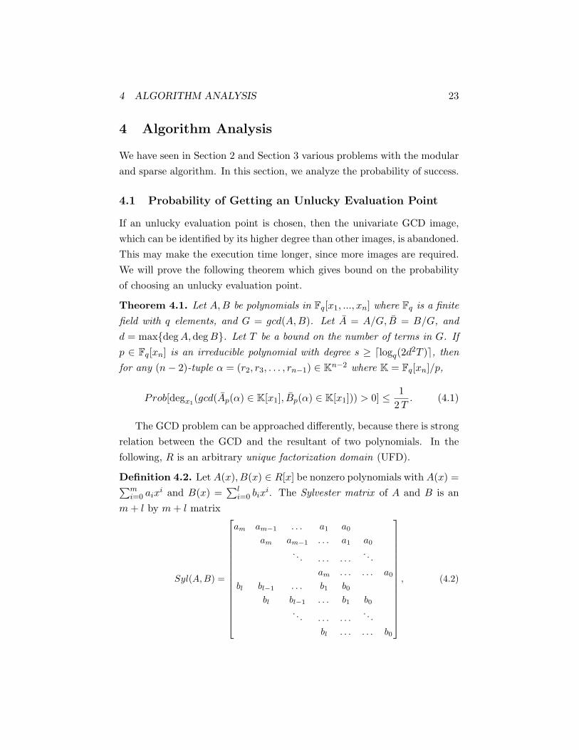
Definition 4.2. Let A(x), B(x) ∈ R[x] be nonzero polynomials with A(x) =∑mi=0 aix
i and B(x) =∑l
i=0 bixi. The Sylvester matrix of A and B is an
m + l by m + l matrix
Syl(A,B) =
am am−1 . . . a1 a0
am am−1 . . . a1 a0
. . . . . . . . .. . .
am . . . . . . a0
bl bl−1 . . . b1 b0
bl bl−1 . . . b1 b0
. . . . . . . . .. . .
bl . . . . . . b0
, (4.2)

4 ALGORITHM ANALYSIS 24
where the upper part of the matrix consists of n rows of coefficients of A(x)and the lower part consists of m rows of coefficients of B(x). The entriesnot shown are zero.
Definition 4.3. Let A(x), B(x) ∈ R[x] be polynomials. The resultant ofA(x) and B(x), denoted by Res(A,B), is the determinant of the Sylvestermatrix of A,B. We also define Res(0, B) = 0 for nonzero B ∈ R[x], andRes(A,B) = 1 for nonzero A,B ∈ R. We write Resx(A,B) if we wish toinclude the polynomial variable.
Proposition 4.4 (Sylvester’s Criterion). [Proposition 8 in Section 3.5from Cox et al. [3]] Given A(x), B(x) ∈ R[x] be polynomials of positive de-gree, the resultant Res(A,B) ∈ R is an integer polynomial in the coefficientsof A and B. Furthermore, A and B have a common factor in R[x] if andonly if Res(A,B) = 0.
To prove Theorem 4.1, we still need one more ingredient, the Schwartz-Zippel Theorem. It is a bound for the probability of encountering a root ofa polynomial. This helps us estimate the probability of choosing unluckyevaluation point.
Theorem 4.5 (Schwartz-Zippel). Let P ∈ F[x1, x2, . . . , xn] be a non-zeropolynomial of total degree d ≥ 0 over a field F. Let S be a finite subset of Fand let r1, r2, . . . , rn be selected randomly from S, then
Prob[P (r1, r2, . . . , rn) = 0] ≤ d
|S|. (4.3)
In our algorithm, evaluation points are randomly chosen from the finitefield K = Fq[xn]/p(xn) where degxn
p = s, i.e., S = K. Since |K| = qs,equation (4.3) can be rewritten as
Prob[P (r1, r2, . . . , rn) = 0] ≤ d
qs. (4.4)

4 ALGORITHM ANALYSIS 25
Remark 4.6. The Schwartz-Zippel Theorem is a tight bound on the proba-bility of getting a zero evaluation point. Consider the following example,
Over F3 :
P = x2 + yx + (y2 + 2)
y = 0 : P = x2 + 2 = (x− 1)(x− 2)
y = 1 : P = x2 + x + 0 = x(x + 1)
y = 2 : P = x2 + 2x = x(x + 2)
We see that Prob[P = 0] =23
=deg(P )| F3 |
.
Proof of Theorem 4.1: By definition, an evaluation α = (r2, r3, . . . , rn−1)is unlucky if degx1
(Ap(α), Bp(α)) > 0. By Proposition 4.4, we know that
degx1(Ap(α), Bp(α)) > 0 ⇐⇒ Resx1(Ap(α), Bp(α)) = 0.
Hence, we need to establish the probability that the Resx1(Ap(α), Bp(α)) =0. We can rearrange the terms of Ap and Bp, and write them in the followingway:
Ap = am(x2, . . . , xn−1)·xm1 +am−1(x2, . . . , xn−1)·xm−1
1 +· · ·+a0(x2, . . . , xn−1)
and
Bp = bl(x2, . . . , xn−1) · xl1 + bl−1(x2, . . . , xn−1) · xl−1
1 + · · ·+ b0(x2, . . . , xn−1)
where ai, bj ∈ K[x2, . . . , xn−1], 1 ≤ i ≤ m, 1 ≤ j ≤ l. The total degree ofeach ai or bj is at most d, since the maximum of the total degrees of A andB are d. The Sylvester Matrix of Ap and Bp in x1 is

4 ALGORITHM ANALYSIS 26
Syl(Ap, Bp) =
am am−1 . . . a1 a0
am am−1 . . . a1 a0
. . . . . . . . .. . .
am . . . . . . a0
bl bl−1 . . . b1 b0
bl bl−1 . . . b1 b0
. . . . . . . . .. . .
bl . . . . . . b0
.
There are m + l rows in Syl(Ap, Bp) and each entry is at most degree d, sototal degree of the determinant r ∈ R[x2, . . . , xn−1] of Syl(Ap, Bp) is,
deg(r(x2, . . . , xn−1)) ≤ (m + l) · d ≤ 2d · d = 2d2. (4.5)
However, the Bezout bound provides a better asymptotic bound, namely
deg(r(x2, . . . , xn−1)) ≤ deg(Ap) · deg(Bp) ≤ d · d = d2. (4.6)
In some cases the Bezout bound may be greater than (m + l) · d , so inpractice one calculates both bounds and uses the minimum of the two. Bythe application of Theorem 4.5 (equation 4.4), we get
Prob [ degx1( gcd(Ap(α), Bp(α)) ) > 0 ] = Prob[r(α) = 0]
≤ d2
|Fq[xn]/p|=
d2
qs≤ d2
qlogq(2d2T )=
d2
2d2T=
12 T
,
because the algorithm chooses s ≥ dlogq 2d2T e.For each sparse interpolation, the algorithm computes at most T uni-
variate image, where T is a bound on the number of terms in G. Thus, theprobability that the algorithm chooses an unlucky evaluation point through-out the whole process is
Prob[choosing an unlucky evaluation point] ≤ T · 12 T
=12.

4 ALGORITHM ANALYSIS 27
4.2 The Probability of a Term Vanishing
In Section 3.3, we mention that if one or more terms are absent from theassumed form Gf , which is calculated from gcd(A/p1, B/p1), then it will leadto a failure and trigger a restart of the algorithm. The following theoremgives a bound on the probability of a failure.
Theorem 4.7. Let A,B be polynomials in Fq[xn][x1, · · · , xn−1] with degree≤ d, and let G = gcd(A,B). Let T be a bound on the number of terms in G.If p ∈ Fq[xn] is an irreducible polynomial with degree s > logq (2 (n− 2)d T ),then at any level of sparse interpolation, for the assumed form Gf ,
Prob [ one or more terms vanish in Gf ] <12. (4.7)
Proof: Consider the situation where the sparse interpolation is appliedon the variable xk+1, i.e., we have obtained the assumed form of G in thevariables x1, . . . , xk. Let X = [x1, . . . , xk] and ei ∈ Zk
≥0 be the degree vector.Then write
G = gt · X et + gt−1 · X et−1 + · · ·+ g0 (4.8)
where gi ∈ Fq[xn][xk+1, . . . , xn−1], and the number of terms, t, is yet todetermined. We want to establish the probability that one or more terms ofG vanish in the assumed form, i.e., the probability that
∃ gi(βk+1, . . . , βn−1) = 0 mod p
for a tuple (βk+1, . . . , βn−1) ∈ Kn−k−1 chosen at random where K = Fq[xn]/p.Note that G = gcd(A,B), so the total degree of G is at most d. Thus,
deg(gi(xk+1, . . . , xn−1)) ≤ d. Since T is a bound on the number of terms inG, then t ≤ T . Therefore, by Theorem 4.5 (Schwartz Theorem), we have
Prob[gi(rk+1, . . . , rn−1) = 0] ≤ d
qs
=⇒ Prob[ one or more gi = 0 ] ≤t∑
i=1
d
qs=
d t
qs≤ d T
qs.

5 EXPERIMENTS ON BENCHMARK EXAMPLES 28
Now consider the whole process where the sparse interpolation is appliedto obtain a GCD using an assumed form Gf . The probability that one ormore terms vanish in any of the Gf ’s throughout the whole process is,
Prob [ one or more terms vanish ]
≤n−1∑k=2
d T
qs
≤ (n− 2)d T
qs
<(n− 2)d T
qlogq(2(n−2)d T )=
(n− 2)d T
2(n− 2)d T=
12,
because s > logq
(2 (n− 2)
(d+n−1
d
)d).
In conclusion for this section, if we choose an irreducible polynomialp ∈ Fq[xn] with degree s > max{logq(2d2T ), logq(2 (n − 2)d T )}, then theprobability of failure due to either unlucky evaluation point or term vanish-
ing is at most12. Since the maximum number of monomials in k variables
of degree ≤ d is(d+n−1
d
), then T ≤
(d+n−1
d
). Thus, we can use
(d+n−1
d
)as a bound on the number of terms of G. However, when G is sparse,T �
(d+n−1
d
). In practice, we choose irreducible polynomial with degree
≥ logq(2d2). When the algorithm encounters unlucky evaluation point orterm vanishing problems, it will trigger a start of the process.
5 Experiments on Benchmark Examples
We implemented our algorithm and other algorithms in Maple using theRECDEN data structure. The fact that this data structure supports multi-ple field extensions over Q and Zp allows our implementation to work overfinite fields and algebraic number fields. We also execute some examples tocompare the time complexity of different approaches.
5 EXPERIMENTS ON BENCHMARK EXAMPLES 29
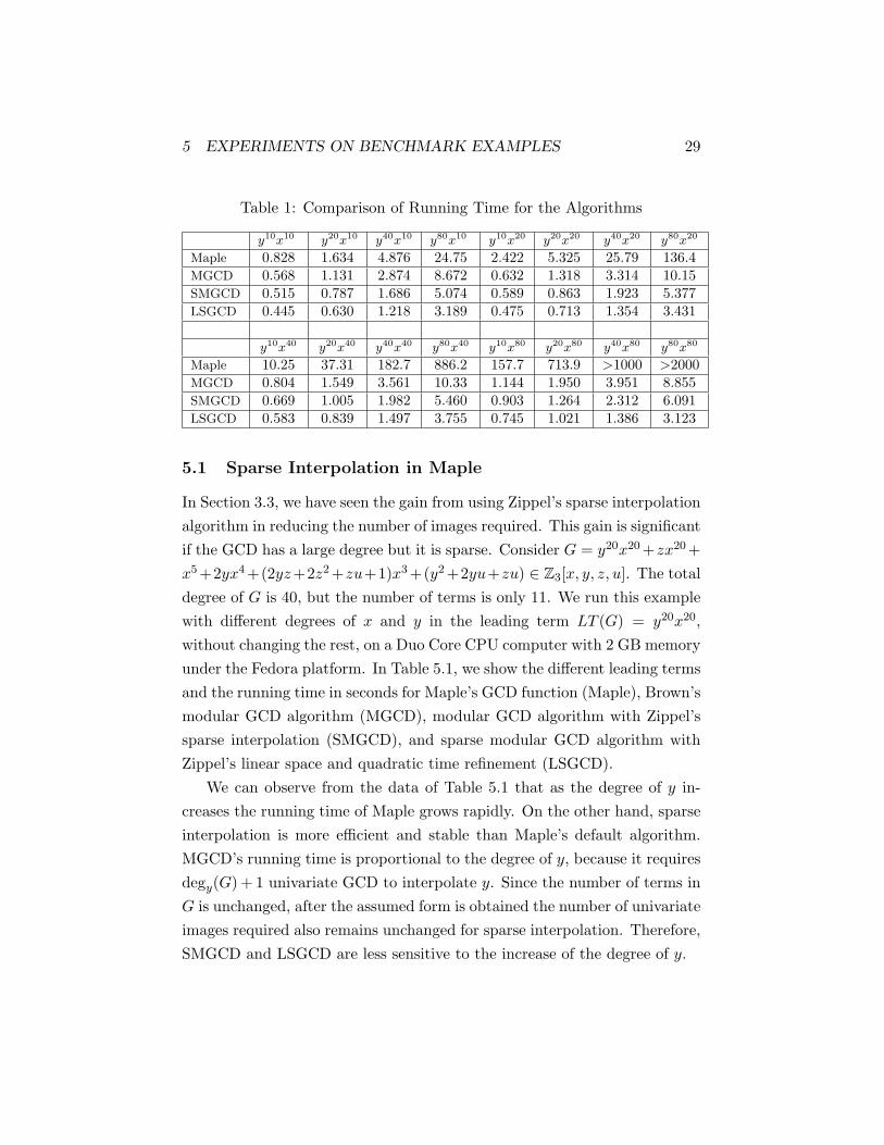
Table 1: Comparison of Running Time for the Algorithms
y10x10 y20x10 y40x10 y80x10 y10x20 y20x20 y40x20 y80x20
Maple 0.828 1.634 4.876 24.75 2.422 5.325 25.79 136.4MGCD 0.568 1.131 2.874 8.672 0.632 1.318 3.314 10.15SMGCD 0.515 0.787 1.686 5.074 0.589 0.863 1.923 5.377LSGCD 0.445 0.630 1.218 3.189 0.475 0.713 1.354 3.431
y10x40 y20x40 y40x40 y80x40 y10x80 y20x80 y40x80 y80x80
Maple 10.25 37.31 182.7 886.2 157.7 713.9 >1000 >2000MGCD 0.804 1.549 3.561 10.33 1.144 1.950 3.951 8.855SMGCD 0.669 1.005 1.982 5.460 0.903 1.264 2.312 6.091LSGCD 0.583 0.839 1.497 3.755 0.745 1.021 1.386 3.123
5.1 Sparse Interpolation in Maple
In Section 3.3, we have seen the gain from using Zippel’s sparse interpolationalgorithm in reducing the number of images required. This gain is significantif the GCD has a large degree but it is sparse. Consider G = y20x20 +zx20 +x5 +2yx4 +(2yz+2z2 +zu+1)x3 +(y2 +2yu+zu) ∈ Z3[x, y, z, u]. The totaldegree of G is 40, but the number of terms is only 11. We run this examplewith different degrees of x and y in the leading term LT (G) = y20x20,without changing the rest, on a Duo Core CPU computer with 2 GB memoryunder the Fedora platform. In Table 5.1, we show the different leading termsand the running time in seconds for Maple’s GCD function (Maple), Brown’smodular GCD algorithm (MGCD), modular GCD algorithm with Zippel’ssparse interpolation (SMGCD), and sparse modular GCD algorithm withZippel’s linear space and quadratic time refinement (LSGCD).
We can observe from the data of Table 5.1 that as the degree of y in-creases the running time of Maple grows rapidly. On the other hand, sparseinterpolation is more efficient and stable than Maple’s default algorithm.MGCD’s running time is proportional to the degree of y, because it requiresdegy(G) + 1 univariate GCD to interpolate y. Since the number of terms inG is unchanged, after the assumed form is obtained the number of univariateimages required also remains unchanged for sparse interpolation. Therefore,SMGCD and LSGCD are less sensitive to the increase of the degree of y.

6 CONCLUSION 30
Table 2: Comparion of SMGCD and LSGCDt = 4 t = 5 t = 6 t = 7 t = 8 t = 9 t = 10 t = 11 t = 12
SMGCD 3.195 3.829 3.846 6.793 7.488 8.258 8.951 9.228 9.466
LNGCD 2.195 2.585 2.689 2.887 3.302 3.766 3.977 4.107 4.281
5.2 Linear Space and Quadratic Time
Since the example in the previous section has no change in the number ofterms, it is not obvious how SMGCD and LSGCD compare to each other.Consider G := (y10 + zy + z + u)x20 + (y10 + zy + z + u + 1)x10 + (y10 +zy2 + z2 + u10)x5 + (z10 + zy)x3 + (y2 + y + z), which has term counts inthe main variable x are n1 = 4, n2 = 4, n3 = 4, n4 = 2, and n5 = 3.
SMGCD and LSGCD use Javadi’s solution to solve the normalizationproblem, so they both choose the coefficients for x3 and x0 to form the firstsystem. We will change the number the terms in the coefficients of x20, x10,and x5, and run SMGCD and LSGCD on it. Table 5.2 shows the runningtime in seconds when we change t = n1 = n2 = n3 from 4 to 12. We canobserve that the running time SMGCD is growing faster than LSMGCDwith respect to the increase in the number of terms.
6 Conclusion
We have successfully modified Zippel’s sparse modular GCD algorithm towork for finite fields with small cardinality. Zippel’s sparse interpolationalgorithm is more efficient than Brown’s algorithm, but may result in afailure that triggers a new call to the algorithm. We analyzed the probabilityof success. If our algorithm chooses an irreducible polynomial from thecoefficient ring with degree large enough, then the probability of unluckyevaluation point and term vanishing problems will be small.
Javadi’s solution for normalization problem with Zippel’s linear spaceand quadratic time refinement make use of Vandermonde matrices, sinceit saves time and space to calculate its inverse. Our algorithm employsa generalized version of the Vandermonde matrix. We introduced a newmaster polynomial which efficiently calculates the inverse of the matrix.

REFERENCES 31
References
[1] W. S. Brown. On Euclid’s Algorithm and the Computation of Poly-nomial Greatest Common Divisors. J. ACM 18, 478-504, 1971.
[2] K. O. Geddes, S. R. Czapor, G. Labahn. Algorithms for ComputerAlgebra. p. 300-335, 1992.
[3] D. Cox, J. Little, D. O’Shea. Ideals, Varieties, and Algorithms. Thirdedition. p. 156, 2007.
[4] M. Javadi. A New Solution to the Polynomial GCD NormalizationProblem. MOCAA M3 Workshop, 2008.
[5] E. Kaltofen, M. B. Monagan. On the Genericity of the Modular Poly-nomial GCD Algorithm. Proceeding of ISSAC ’99, ACM Press, 59-66,1999.
[6] J. de Kleine, M. B. Monagan, A. D. Wittkopf. Algorithms for theNon-monic Case of the Sparse Modular GCD Algorithm. Proceedingof ISSAC ’05, ACM Press, pp. 124-131 , 2005.
[7] R. Zippel. Probabilistic Algorithms for Sparse Polynomials, P. EU-ROSAM ’79, Springer-Verlag LNCS, 2, 216-226, 1979.
[8] R. Zippel. Interpolating Polynomials from their Values. J. SymbolicComp. 9(3), 375-403, 1990.