Computing the channel capacity of a communication system

affected by uncertain transition probabilities

Krzysztof Postek 1 Aharon Ben-Tal 2

Abstract

We study the problem of computing the capacity of a discrete memoryless channel under

uncertainty affecting the channel law matrix, and possibly with a constraint on the average

cost of the input distribution. The problem has been formulated in the literature as a max-

min problem. We use the robust optimization methodology to convert the max-min problem

to a standard convex optimization problem. For small-sized problems, and for many types of

uncertainty, such a problem can be solved in principle using interior point methods (IPM).

However, for large-scale problems, IPM are not practical. Here, we suggest an O(1/T )

first-order algorithm based on [10] which is applied directly to the max-min problem.

1 Introduction

Channel capacity is a fundamental notion in the field of information theory that started

with the seminal paper of [12]. For a given channel, it provides an upper bound on the rate

at which information can be reliably transmitted. In this paper we consider the problem

of computing the capacity of a discrete memoryless channel (DMC). A DMC consists of an

input alphabet of N symbols, each used with probability pn determined by the user, and an

output alphabet Y of M symbols. Given the n-th input symbol, the m-th output symbol

occurs with a conditional probability Qnm, where the matrix Q ∈ RN×M is known as the

channel law matrix. The channel capacity of a DMC is given by:

(CC) supp∈∆N

I(p,Q) := supp∈∆m

N∑n=1

M∑m=1

pnQnm logQnm

N∑l=1

plQlm

,

where the maximized term is known as the average mutual information (AMIM). The AMIM

is a convex function of the input distribution p and hence, at least in theory, convex opti-

mization algorithms can be used to solve (CC). However, the performance of such algorithms

can be poor and the need for other approaches emerged. One of the first algorithms is the

well-known Arimoto-Blahut algorithm (see [1; 6]). Later, more efficient algorithms have been

developed to solve the capacity problem and some of its special cases. A comprehensive sur-

vey of algorithms for solving (CC) is given in [13]. This paper also suggests a first-order

algorithm based on [11] for problem (CC) with an additional linear constraint.

In reality, channels correspond to physical devices affected by inaccuracies and/or whose

parameters are measured only up to a certain accuracy. Therefore, the channel at hand

1Faculty of Industrial Engineering and Management, Technion - Israel Institute of Technology, e-mail:

krzysztofp@technion.ac.il2Faculty of Industrial Engineering and Management, Technion - Israel Institute of Technology; Shenkar College,

Israel, e-mail: abental@ie.technion.ac.il

1

may differ from its assumed version. Already in the 1950’s researchers were considering the

possibility that the channel is not known fully. This case, known as compound channel case,

has a rich literature, see e.g. [5; 8; 14]. A comprehensive survey by [9] summarizes these

results. In this paper, the uncertain channel capacity problem is represented as:

(R-CC) supp∈∆m

infQ∈Q

I(p,Q),

where the channel law matrix Q is only known to belong to a set Q. In today’s language (R-

CC) could be called a robust optimization problem [3; 4] where Q is the so-called uncertainty

set. To the best of our knowledge, there are no papers in the literature on algorithms for

solving (R-CC). The main purpose of our paper is to fill this gap by designing an efficient

algorithm for solving large scale instances. Contrary to [13], we cannot use the algorithm

of [11] since the coupling term in (R-CC) is not bilinear. Instead, we propose a first-order

algorithm based on [10]. The performance of this algorithm relies on two types of operation

that need to be executed in each iteration. The first of them is the computation of the

gradient of the AMIM with respect to p and Q. Secondly, at each iteration the algorithm

calls an oracle consisting of a proximal minimization. We show that for our problem, an

analytic expression for the minimum is obtained, or the proximal minimization reduces to

solving a single-variable convex problem.

The contribution of our paper is as follows:

• we show that the robust counterpart (RC) of the min-max problem (R-CC) reduces

to a standard deterministic convex optimization problem. Moreover, we derive a dual

form of RC. For the binary symmetric channel, this reduces to an explicit formula

and for a weakly symmetric channel with Kullback-Leibler uncertainty it reduces to a

single-variable problem;

• we adapt the algorithm of [10] to (R-CC) and derive simple conditions under which the

O(1/T ) convergence can be proved;

• similar to Sutter et al. [13], we look at an extended version of problem (R-CC) which

includes an average cost constraint, and we show how to extend the algorithm to handle

this case;

• by numerical experiments, we illustrate the effect of uncertainty on the channel capacity.

The organization of the paper is as follows. In Section 2 we derive the convex formulation of

the uncertain channel capacity problem and its dual. In Section 3 we adapt the algorithm

of [10] to solve the uncertain channel capacity problem for large-scale instances. Section 4

includes three numerical experiments illustrating the impact of uncertainty on channel ca-

pacity.

Notation. We denote by ∆N the N -dimensional simplex and by ∆N×M is a set of

matrices where each row belongs to ∆M . C1,1(A) shall denote the space of differentiable

functions with a Lipschitz continuous gradient over the set A. By ∂g(λ) we denote the

subdifferential of function g(·) at point λ. For a norm ‖ · ‖ we denote by ‖ · ‖∗ its dual norm.

2 The uncertain channel capacity problem

2.1 Deriving the robust counterpart (RC)

The RC is derived by dualizing the inner problem in the min-max (R-CC) (Proposition 1).

This results in a standard maximization of a concave function over a convex set.

2

Proposition 1 Let the uncertainty set Q ⊂ RN×M be a compact convex set. Then, the

worst-case capacity of a channel is given by the optimal value to the following problem:

maxp,λ,V

N∑n=1

λn − δ∗(V |Q) (P)

s.t.

N∑n=1

pn exp

(λn − Vnm

pn

)≤ 1, ∀m

p ≥ 0

N∑n=1

pn = 1,

where δ∗(V |Q) is the support function of the set Q evaluated at V ∈ RN×M .

Proof. We begin by deriving the dual of the inner problem in (R-CC). Let:

f(Q, p) =

N∑n=1

M∑m=1

pnQnm logQnm

N∑l=1

plQlm

.

Using the results of [4], relying on Fenchel duality, we have:

infQ∈Q

f(Q, p) = infQ{f(Q, p) + δ (Q|Q)}

= infQ{δ (Q|Q)− (−f(Q, p))}

= supV

{(−f)∗(V, p)− δ∗ (V |Q)} , (1)

where (−f)∗(V, p) is the concave conjugate of the function −f with respect to the first vari-

able and δ∗ (V |Q) is the support function of the set Q, evaluated at V ∈ RN×M . Therefore,

we need to find:

(−f)∗(V, p) = infQ∈∆N×M

N∑n=1

M∑m=1

pnQnm logQnm

N∑l=1

plQlm

+ VnmQnm

(2)

So, let us define new variables:

xnm = pnQnm, ∀n,m, qm =

N∑n=1

pnQnm

in terms of which

infQ∈∆N,M

N∑n=1

M∑m=1

pnQnm logQnm

N∑l=1

plQlm

+ VnmQnm

is equivalent to

infxnm,qm

−N∑n=1

pn log pn +

N∑n=1

(M∑m=1

xnm logxnmqm

+ Vnmxnmpn

)

s.t.

M∑m=1

xnm = pn ∀n

q ∈ ∆M

xnm ≥ 0 ∀n,m.

3

Next, we use Lagrangian duality to compute the dual of the latter problem :

infq∈∆M ,xnm≥0

N∑n=1

M∑m=1

(xnm log

xnmqm

+ VnmQnm

)−

N∑n=1

un

(∑m

xnm − pn

)

=

N∑n=1

unpn + infq∈∆n

infxnm≥0

N∑n=1

M∑m=1

qm

(xnmqm

logxnmqm− xnm

qm

(un −

Vnmpn

))

=

N∑n=1

unpn + infq∈∆n

N∑n=1

M∑m=1

qm exp

(un −

Vnmpn− 1

)

=

N∑n=1

unpn −maxm

N∑n=1

exp

(un −

Vnmpn− 1

)Introducing an auxiliary variable µ for the max term and using strong duality, we obtain:

(−f)∗(V, p) = maxun,µ

−N∑n=1

pn log pn +

N∑n=1

unpn − µ

s.t. µ ≥N∑n=1

exp

(un −

Vnmpn− 1

)∀m.

We introduce auxiliary variable λn such that un = log pn + λn/pn + µ to obtain

(−f)∗(V, p) = maxλ,µ

N∑n=1

λn

s.t. µ ≥N∑n=1

pn exp

(λn − Vnm

pn− 1 + µ

)∀m.

Each of the constraints has a form µ ≥ A exp(µ) where A > 0. The property of such a

constraint is:

A ≥ A′ > 0 ⇒ (µ ≥ A exp(µ) ⇒ µ ≥ A′ exp(µ)) .

Therefore, if there exists a µ satisfying one of the constraints for which the expression∑N

n=1 pn exp ((λn − Vnm)/pn − 1) is smallest, this µ satisfies all of the constraints. Therefore:

µ ≥N∑n=1

pn exp

(λn − Vnm

pn− 1 + µ

)∀m ⇔ µm ≥

N∑n=1

pn exp

(λn − Vnm

pn− 1 + µm

)∀m

and one can eliminate µm from each inequality by moving the terms to the left-hand side

and maximizing w.r.t. µm. In the end, we obtain:

(−f)∗(V, p) = maxλ

N∑n=1

λn

s.t.

N∑n=1

pn exp

(λn − Vnm

pn

)≤ 1 ∀m.

This expression is inserted back into (1), which in turn inserted into (R-CC) results in the

final form (P). �

Problem (P) is convex – the objective is a concave function of the decision variables and

the first constraint involves the perspectives of the (convex) exponential function. Thus if the

support function δ∗(·|Q) has a tractable form (see e.g. [4] for a review of computationally

tractable uncertainty sets), it can be solved using convex optimization methods, e.g., the

IPM. In the next section, we derive the problem dual to (P) which allows us to obtain upper

bounds on the robust channel capacity.

4

Remark 1 In [13], the deterministic channel capacity problem includes a linear average cost

constraint. It models the case where use of the n-th symbol of the input alphabet incurs a

cost an and the aim is to keep the average cost below a threshold b. This gives a constraint

a>p ≤ b, where a ∈ RN+ and b ∈ R+. In our robust setting, such a constraint is also easily

included as it is sufficient to append it to problem (P).

2.2 Dual problem

The following proposition gives the convex optimization problem dual to (P).

Proposition 2 A dual of problem (P) for which strong duality holds is given by:

minv,Q

log

M∑m=1

exp(vm) + maxn

{M∑m=1

Qnm(logQnm − vm)

}(D)

s.t. Q ∈ Q.

Proof. See Appendix A.1. �

The following corollary gives an upper bound on the robust channel capacity by inserting

the feasible solution vm = log∑

lQlm.

Corollary 1 The following is an upper bound on the robust channel capacity (R-CC):

min(D) ≤ minQ∈Q

logN + maxn

M∑m=1

Qnm logQnm∑l

Qlm

(3)

As it turns out, the upper bound of Corollary 1 is tight for the class of weakly symmetric

channels.

Definition 1 A channel is weakly symmetric if each row contains the same set of values

as any other row, with possible permutations, and the column sums are equal.

For example, the following channel is weakly symmetric:

Q =

[13

16

12

13

12

16

]and the following uncertainty set involves only weakly symmetric channels:

Q = conv

([13

16

12

13

12

16

],

[13

12

16

13

16

12

]).

For weakly symmetric channels, it is sufficient to specify an uncertainty set forQ by specifying

the uncertainty set for a single row (with permuted values of the same entries in other rows)

with the condition that the sums of the column entries stays equal.

Proposition 3 For weakly symmetric channels the bound (3) is tight:

min(D) = minQ∈Q

logN +

M∑m=1

Q1m logQ1m∑l

Qlm

. (4)

Proof. See Appendix A.2. �

2.3 Special cases

As an illustration of the results, we consider two simple cases: (i) the well-known binary sym-

metric channel, and (ii) the weakly symmetric channel under Kullback-Leibler uncertainty

about the transition probabilities in each row of Q.

5

2.3.1 Binary symmetric channel

A binary symmetric channel is one where m = n = 2 and

Q =

[1− β β

β 1− β

].

Clearly, this channel is characterized by a single parameter β and hence, the only possible

compact convex uncertainty set is an interval β ∈ [β, β]. Then, the following result holds:

Proposition 4 Assume w.l.o.g. that β ≤ 1/2. Then, the robust capacity of a binary sym-

metric channel is given by

log 2 + β∗ log β∗ + (1− β∗) log(1− β∗) where β∗ = min{1/2, β}.

Proof. See Appendix A.3. �

2.3.2 Weakly symmetric channels under Kullback-Leibler (KL) uncer-

tainty

Weak symmetry allows us to focus on a single row, so let us define rm = Q1m and∑N

l=1Qlm =

N/M for all m. Under KL uncertainty, the uncertainty set for the first row is given as:

Q =

{r ∈ RM+ : 1>r = 1,

M∑m=1

rm log

(rmqm

)≤ ρ

}.

In this setting, the dual problem (D) reduces to the following one:

minrn

logN +

M∑m=1

rm logrmN/M

minrn

logM +

M∑m=1

rm log rm

s.t.

M∑m=1

rm log

(rmqm

)≤ ρ ⇔ s.t.

M∑m=1

rm log

(rmqm

)≤ ρ

M∑m=1

rm = 1

M∑m=1

rm = 1

rm ≥ 0 rm ≥ 0.

Omitting the first term logM , we write the Lagrangian and minimize w.r.t. rm to obtain

the dual function:

g(µ, λ) = infrm≥0

M∑m=1

rm log rm + λ

(M∑m=1

rm log

(rmqm

)− ρ

)+ µ

(M∑m=1

rm − 1

)

= infrm≥0

M∑m=1

(1 + λ)rm log rm − (λ log qm − µ)rm − λρ− µ

which by optimizing w.r.t. rm gives

=−M∑m=1

(1 + λ) exp

(λ log qm − µ

1 + λ− 1

)− λρ− µ,

where λ ≥ 0. To solve the dual problem maxµ,λ≥0 g(µ, λ) we maximize first w.r.t. µ to obtain

the optimality condition:

dg(µ, λ)

dµ= 0 ⇔ −

M∑m=1

exp

(λ log qm − µ

1 + λ− 1

)+1 = 0 ⇔ µ = (1+λ) log

(M∑m=1

exp

(λ log qm1 + λ

− 1

)),

6

which, after inserting it back, gives the following maximization problem over a single variable

λ ≥ 0:

maxλ≥0

−M∑m=1

(1 + λ) exp

λ log qm − (1 + λ) log

(M∑m=1

exp(λ log qm

1+λ− 1))

1 + λ

−λρ− (1 + λ) log

(M∑m=1

exp

(λ log qm1 + λ

− 1

))}.

3 A proximal algorithm for solving the robust channel

capacity problem (R-CC)

3.1 Introduction

In principle, the robust channel capacity problem of Proposition 1 can be solved using the

interior point methods for a wide range of convex and compact uncertainty sets Q. However,

the numerical performance of these methods is poor already on medium-sized instances

which is in line with the experience already gained in the deterministic case [13]. This is

particularly due to the presence of the variable matrix V ∈ RN×M , which greatly increases

the computational effort since the IPMs in each iteration require solving a linear system

of size corresponding to the number of variables. This situation calls for using first-order

methods.

It turns out that in a suitable uncertainty setting, the original max-min problem (R-CC)

can be solved using the prox-algorithm of [10]. The algorithm has a convergence rate of

O(1/T ) and its performance relies on two types of operation that need to be executed in

each iteration: (i) computing the gradient of the AMIM with respect to p and Q; (ii) calling

an oracle which performs a proximal minimization step. For the max-min problem (R-CC)

the partial derivatives of the AMIM with respect to p and Q are easily computed. As for the

proximal minimization, an analytic expression for the minimum is obtained, or the proximal

minimization reduces to solving a single-variable convex problem.

In Appendix B we state a self-contained description of the algorithm of [10]. Here,

we first present our modelling setup and show that it satisfies the crucial assumptions for

proving the convergence of the algorithm. In Section 3.2 we outline the algorithm and state

its convergence. In Section 3.3 we extend the algorithm to the case with the average cost

constraint added.

We propose a rather general modeling setup where the uncertainty set for the channel

law matrix Q is given as:

Q =

{Q(ξ) : Q(ξ) = Q0 +

S∑s=1

ξsQs, ξ ∈ B

},

where B ⊂ RS is a ‘simple’ compact convex set of perturbations ξ. By ‘simple’ it is meant

that it is easy to perform the proximal minimization step. Examples of such simple B are:

∞-norm ball, 2-norm ball, and simplex. For the first two cases, we add to the description of

the Q constraints Qs1 = 0 for all s = 1, . . . , S, necessary for the row sums of Q(ξ) to stay

equal to 1 for all ξ ∈ B.

In this setup, the problem to solve is:

maxp∈∆N

minξ∈B

φ(ξ, p) = minξ∈B

maxp∈∆N

φ(ξ, p), (5)

7

where

φ(ξ, p) =

N∑n=1

M∑m=1

pnQnm(ξ) logQnm(ξ)

N∑l=1

plQlm(ξ)

and where the fact that the max-min = min-max holds due to the Sion-Kakutani minimax

theorem. We set z = (ξ, p) to shorten the notation and define the gradient mapping

Φ(z) =

[∇ξφ(z)

−∇pφ(z)

].

The three crucial assumptions for the algorithm’s convergence are: (i) compactness of the

domain, (ii) Lipschitz continuity of Φ(z), (iii) existence of strongly convex distance-generating

functions that it is easy to minimize them over the domain.

The compactness assumption (i) is satisfied due to the compactness of B and ∆N . As-

sumption (ii) can be easily met due to the following result.

Proposition 5 If for some τ > 0 it holds that Qnm > τ for all Q ∈ Q, then the mapping:

Ψ(Q, p) =

[∇Qf(Q, p)

∇pf(Q, p)

]

is Lipschitz continuous on Q×∆N . �

Proof. See Appendix A.4. �

Remark 2 Note the extra assumption τ > 0. A similar assumption is made in the deter-

ministic channel case of [13], in order to force the set of dual solutions of a certain problem

to be compact, on which the convergence of their algorithm rests.

The third assumption (iii) is the existence of a distance-generating function ω : Rn×Rm+ → Rsuch that the computation of the proximal operator:

Proxz(d) = arg minw∈B×∆N

[ω(w) + 〈w, d− ω′(z)〉] .

is simple. In line with [10], we use

ω(z) = γ1ω1(ξ) + γ2ω2(p) (6)

where ω1(·) and ω2(·) are strongly convex distance-generating functions over B and ∆N and

γ1, γ2 are suitably chosen positive constants. Possible choices for ω1(·) and ω2(·) are:

• ω1(·):

for B – ∞-norm ball or 2-norm ball:

ω1(ξ) =ξ>ξ

2,

for B – simplex:

ω1(ξ) =

S∑s=1

(ξs + δ/S) log(ξs + δ/S),

where δ > 0 is an arbitrarily positive number.

• ω2(·):

ω2(p) =

N∑n=1

(pn + δ/N) log(pn + δ/N).

8

With such a choice, the computation of the prox-operator is equivalent to:

minw∈B×∆N

[ω(w) + 〈w, d− ω′(z)〉] (7)

= minξ∈B,p∈∆N

[γ1ω1(ξ) + γ2ω2(p) +

⟨[ξ

p

],

[d1

d2

]−

[γ1ω

′1(z)

γ2ω′2(z)

]⟩],

and can be done easily. Indeed, one can minimize (7) over p and ξ separately to obtain:

pn = max

{0, exp

(−1− µ− d2n − γ2ω

′2n(z)

γ2

)− δ

N

}(8)

where µ is the solution to the single-variable equation:

N∑n=1

max

{0, exp

(−1− µ− d2n − γ2ω

′2n(z)

γ2

)− δ

N

}= 1.

For minimization over ξ we have the following three cases corresponding to the different

choices for ω1(·):

• B – ∞-norm ball:

ξk =

−1 if

γ1ω′1k(z)−d1kγ1

< −1γ1ω′1k(z)−d1kγ1

if − 1 ≤ γ1ω′1k(z)−d1kγ1

≤ 1

1 ifγ1ω′1k(z)−d1kγ1

> 1,

• B – 2-norm ball:

ξ =

γ1ω′1(z)−d1γ1

if∥∥∥ γ1ω′1(z)−d1

γ1

∥∥∥2≤ 1

γ1ω′1(z)−d1

‖γ1ω′1(z)−d1‖2

otherwise,

• B – simplex is analogous to (8).

3.2 The algorithm and its convergence

Now, we present the scheme of the algorithm. Each general step is illustrated with the specific

case where B is the ∞-norm ball, ω1(ξ) = ξ>ξ/2 and ω2(p) =N∑n=1

(pn + δ/N) log(pn + δ/N).

1. Initialize with a point (ξ0, p0) = z0 ∈ Z = B ×∆N .

2. Given zt−1, check if

zt−1 = Proxzt−1(Φ(zt−1)).

In our example, this reduces to solving the problem:

w = arg minξ∈B,p∈∆N

[γ1

ξ>ξ

2+ γ2

N∑n=1

(pn + δ/N) log(pn + δ/N)

+

⟨[ξ

p

],Φ(zt−1)−

[γ1ξ

γ2(1 + log(p+ δ/N))

]⟩]

and checking if w = zt−1.

If equality holds, the algorithm stops and zt−1 is the saddle point in (5). Otherwise,

go to Step 3.

3. Choose a γt > 0, set wt,0 := zt−1 and do the inner iteration (over k = 1, 2, . . .):

wt,k = Proxzt−1(γtΦ(wt,k−1)). (9)

9

until for the first time the following inequality holds:⟨γtΦ(wt,k−1), wt,k−1 − wt,k

⟩+ ω(zt−1) +

⟨ω′(zt−1), wt,k − zt−1

⟩− ω(wt,k−1) ≤ 0.

(10)

In our example, this means solving the problem:

w = arg minξ∈B,p∈∆N

[γ1

ξ>ξ

2+ γ2

N∑n=1

(pn + δ/N) log(pn + δ/N)

+

⟨[ξ

p

], γtΦ(wt,k−1)−

[γ1ξ

t,k−1

γ2(1 + log(pt,k−1 + δ/N))

]⟩]until it holds that:⟨γtΦ(wt,k−1), wt,k−1 − wt,k

⟩+ γ1(ξt−1)>ξt−1 + γ2

N∑n=1

(pt−1n + δ/N) log(pt−1

n + δ/N)

+⟨zt−1, wt,k − zt−1

⟩− γ1(ξt,k−1)>ξt,k−1 − γ2

N∑n=1

(pt,k−1n + δ/N) log(pt,k−1

n + δ/N) ≤ 0.

When the inner iteration is finished and condition (10) is satisfied, run the following

updates:

wt = wt,k−1

zt = wt,k

yt =

∑t

l=0 γlwl∑t

l=1 γl,

where yt is the approximate solution to (5), and go back to Step 1.

The algorithm’s complexity is stated in the following proposition based on Proposition 2.2

in [10].

Proposition 6 Let α1, α2 > 0 be the strong convexity parameters of ω1(ξ), ω2(p), ‖ · ‖(1)

and ‖ · ‖(2) be two norms and Luv > 0, u, v ∈ {1, 2} such that:

Luv ≥‖∇zuφ(z)−∇zuφ(z′)‖(u)∗

‖zv − z′v‖(v),∀z, z′ ∈ B ×∆N , zv 6= z′v, zu = z′u,

and

Θ1 ≥ supξ,ξ′∈B

{ω1(ξ)−ω1(ξ′)−〈ξ − ξ′, ω′1(ξ′)〉}, Θ2 ≥ supp,p′∈∆N

{ω2(p)−ω2(p′)−〈p− p′, ω′2(p′)〉},

and γ1, γ2 in (6) be equal to:

γ1 =

2∑l=1

L1l

√Θ1Θl

α1αl

Θ1

2∑k=1

2∑l=1

Lkl

√ΘkΘl

αkαl

, γ2 =

2∑l=1

L2l

√Θ2Θl

α2αl

Θ2

2∑k=1

2∑l=1

Lkl

√ΘkΘl

αkαl

,

and γt satisfy the following condition for all iterations t:

γt ≤ 1√

22∑

k=1

2∑l=1

Lkl

√ΘkΘl

αkαl

,

Under these assumptions, in each iteration t there are at most two inner iterations (9) and

the number T of iterations to obtain an ε-approximation of the solution to (5) is

O

((2∑

k=1

2∑l=1

Lkl

√ΘkΘl

αkαl

)/ε

).

�

10

The cost of each iteration is O(NMS) – it consists of computing the derivatives of φ w.r.t.

ξ and p and computing the proximal operator at most a fixed number of times. The total

complexity depends on the dependence of the terms Θ1, α1 on S. For example, if B is chosen

to be an S-dimensional Euclidean ball, the complexity is:

O (NMS logN/ε) .

Remark 3 In the experiments, we observe a strong dependence of the convergence speed on

the parameters γt. The observed convergence is faster if γt is larger. However, a small γt

is needed to guarantee that the number of inner iterations is at most 2. For that reason, we

implemented an update rule multiplying γt by 1.5 if the number of inner iterations was at

most 2, and dividing it by 1.5 otherwise. This heuristic performed well in our computational

study.

3.3 Average cost constraint

A practically relevant extension of (CC) is the situation where there is a constraint on the

average cost of the input distribution [13]. In such case, the feasible set of p is ∆N = {p ∈RN+ : 1>p = 1, a>b ≤ b} and the worst-case channel capacity is equal to:

minQ∈Q

maxp∈∆N

N∑n=1

M∑m=1

pnQnm logQnm

N∑l=1

plQlm

(11)

Our goal is to solve (11) efficiently with the same machinery as the basic algorithm. Hence, we

want to transform (11) to a saddle point problem where the maximization and minimization

are done over compact sets for which it is still easy to compute the proximal operators. To

do this, we make the following mild assumption and recall a well-known property of the

average mutual information.

Assumption 1 The inner problem in (11) is strictly feasible and its holds that minn an < b

and maxn an > b. �

Property 1 (See [7]) It holds that:

0 ≤N∑n=1

M∑m=1

pnQnm logQnm

N∑l=1

plQlm

≤ min {logN, logM} .

By dualizing the inner problem in (11) w.r.t. the average cost constraint, we obtain the

following problem, which by Assumption 1 and strong duality is equivalent to (11):

infQ∈Q

infλ≥0

supp∈∆N

N∑n=1

M∑m=1

pnQnm logQnm

N∑l=1

plQlm

+ λ

(b−

N∑n=1

pnan

)(12)

The expression in (12) is convex in (Q,λ) and concave in p. However, the domain for λ is

unbounded whereas the use of the algorithm of [10] requires compactness of the domain in

both p and (Q,λ). A way to ensure it is to find a Λ such that λ∗ ≤ Λ. To find such a Λ, we

fix some Q ∈ Q and consider the maximized function of λ in (12):

g(λ) = supp∈∆N

N∑n=1

M∑m=1

pnQnm logQnm

N∑l=1

plQlm

+ λ

(b−

N∑n=1

pnan

). (13)

11

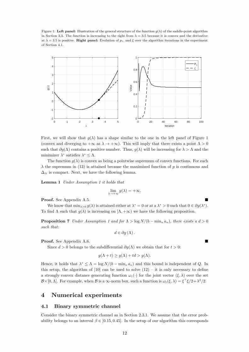
Figure 1: Left panel: Illustration of the general structure of the function g(λ) of the saddle-point algorithm

in Section 3.3. The function is increasing to the right from λ = 3.5 because it is convex and the derivative

at λ = 3.5 is positive. Right panel: Evolution of p1, and ξ over the algorithm iterations in the experiment

of Section 4.1.

0 20 40 60 80 100

Iteration

0

0.2

0.4

0.6

0.8

1

Val

ue

p1

ξ

0 1 2 3 4 5

λ

-2

-1

0

1

2

3

4

5

g(λ

)

First, we will show that g(λ) has a shape similar to the one in the left panel of Figure 1

(convex and diverging to +∞ as λ→ +∞). This will imply that there exists a point Λ > 0

such that ∂g(Λ) contains a positive number. Thus, g(λ) will be increasing for λ > Λ and the

minimizer λ∗ satisfies λ∗ ≤ Λ.

The function g(λ) is convex as being a pointwise supremum of convex functions. For each

λ the supremum in (13) is attained because the maximized function of p is continuous and

∆N is compact. Next, we have the following lemma.

Lemma 1 Under Assumption 1 it holds that

limλ→+∞

g(λ) = +∞.

Proof. See Appendix A.5. �

We know that minλ≥0 g(λ) is attained either at λ∗ = 0 or at a λ∗ > 0 such that 0 ∈ ∂g(λ∗).

To find Λ such that g(λ) is increasing on [Λ,+∞) we have the following proposition.

Proposition 7 Under Assumption 1 and for Λ > logN/(b−minn an), there exists a d > 0

such that:

d ∈ ∂g (Λ) .

Proof. See Appendix A.6. �

Since d > 0 belongs to the subdifferential ∂g(Λ) we obtain that for t > 0:

g(Λ + t) ≥ g(Λ) + td > g(Λ).

Hence, it holds that λ∗ ≤ Λ = logN/(b −minn an) and this bound is independent of Q. In

this setup, the algorithm of [10] can be used to solve (12) – it is only necessary to define

a strongly convex distance generating function ω1(·) for the joint vector (ξ, λ) over the set

B×[0,Λ]. For example, when B is a∞-norm box, such a function is ω1(ξ, λ) = ξ>ξ/2+λ2/2.

4 Numerical experiments

4.1 Binary symmetric channel

Consider the binary symmetric channel as in Section 2.3.1. We assume that the error prob-

ability belongs to an interval β ∈ [0.15, 0.45]. In the setup of our algorithm this corresponds

12

to the channel law matrix:

Q(ξ) = Q0 + ξQ1, Q0 =

[0.7 0.3

0.3 0.7

], Q1 =

[−0.15 0.15

0.15 −0.15

], ξ ∈ [−1, 1].

We run the proximal algorithm with starting point p0 = (0.9, 0.1)> and ξ0 = 0. By Propo-

sition 4 we know that the saddle point corresponds to p = (0.5, 0.5)> and ξ = 1. The

right panel of Figure 1 illustrates the evolution of the decision variables over the first 100

iterations.

4.2 Impact of uncertainty

The next example illustrates the impact of uncertainty on channel capacity. Consider the

deterministic channel to be a randomly generated one, with a nominal channel law matrix

Q0 with N = M = 50 simulated randomly as:

Q0nm =

W 4nm

M∑l=1

W 4nl

, Wnm ∼ U([1, 6.7]) ∀n,m.

This way of sampling has two purposes: (i) keeping all the entries of Q0nm ≥ 10−5, (ii)

reducing the number of ‘dominant’ entries per row by using the 4-th power.

We define the uncertainty as follows:

Q(ξ) = Q0 +

S∑s=1

ξsQsnm, ξ ∈ B,

where

Qsnnm = Γ

(1

M−Q0

nm

)B = {ξ ∈ RS : 0 ≤ ξs ≤ 1, ∀s, ‖ξ‖2 ≤ 1},

where 0 ≤ Γ ≤ 1 and sn, n = 1, . . . , N are sampled independently and uniformly from

{1, 2, . . . , S}. In words, there are S underlying primitive uncertainties ξs and the ambiguity

setup allows the perturbed channel to approach the channel in which every row of the channel

law matrix is uniformly distributed, and the maximum size of perturbation is controlled by

Γ. The Euclidean norm of the perturbation vector ξ is restricted to be no greater than 1,

so that not all components ξs can attain value 1 simultaneously. In the numerical setup we

take S = 5.

Additionally, we consider the version of this problem with additional average cost con-

straint a>p ≤ b. We set b = 1 and the n-component of a is given by:

an =

{50 if pn ≥ 0.05

0 otherwise,

where p is the optimal solution to the problem without the constraint. In this way, we impose

a very high penalty on the 10 input symbols whose optimal probability in the problem without

the linear constraint was larger than or equal to 0.05.

The left panel in Figure 2 illustrates the change in the channel capacity for the problem

without and with the average cost constraint. We observe that the capacity of the channel

drops significantly as the uncertainty scaling parameter Γ increases. We see also that the

capacity of the channel with the average cost constraint is strictly smaller than of the channel

without such a constraint for all Γ.

4.3 Channel affected by a single uncertainty

Next we consider an experiment such that the channel is affected by a single large source of

uncertainty and the idiosyncratic uncertainties of each row are negligible.

13

Figure 2: Left panel: Worst-case channel capacities as a function of Γ in the example of Section 4.2

– without and with the average cost constraint. Right panel: Worst-case channel capacities and the

capacity for the deterministic channel (with ξ = 0) in the example of Section 4.3. Capacities computed up

to 0.01 accuracy.

0 0.2 0.4 0.6 0.8 1

Γ

0

0.2

0.4

0.6

0.8C

apac

ity

No constraintAvg cost constraint

0 10 20 30 40 50

W

2.5

3

3.5

Cap

acity

UncertainDeterministic

We consider an uncertain channel with N = M > 4 where:

Q(ξ) = Q0 + ξQp,

where ξ ∈ [−1, 1] and the matrices are defined as:

Q0 =

0.92 − (m− 5)τ 0.02 0.02 0.02 0.02 τ · · ·0.02 0.92 − (m− 5)τ 0.02 0.02 0.02 τ · · ·0.02 0.02 0.92 − (m− 5)τ 0.02 0.02 τ · · ·

τ · · · 0.02 0.02 0.92 − (m− 5)τ 0.02 0.02

· · · τ 0.02 0.02 0.02 0.92 − (m− 5)τ 0.02

· · · τ 0.02 0.02 0.02 0.02 0.92 − (m− 5)τ

where τ = 10−5 and the perturbation matrix is

Qp =

0.07w1 0.0175w1 0.0175w1 0.0175w1 0.0175w1 0 · · ·0.0175w2 0.07w2 0.0175w2 0.0175w2 0.0175w2 0 · · ·0.0175w3 0.0175w3 0.07w3 0.0175w3 0.0175w3 0 · · ·

· · · 0 0.0175wm−2 0.0175wm−2 0.07wm−2 0.0175wm−2 0.0175wm−2

· · · 0 0.0175wm−1 0.0175wm−1 0.0175wm−1 0.07wm−1 0.0175wm−1

· · · 0 0.0175wm 0.0175wm 0.0175wm 0.0175wm 0.07wm

.

The nominal matrix Q0 reflects the possible events following the choice of the n-th input

symbol:

• the output symbol is the n-th output symbol with probability 0.92− (N − 5)τ ;

• the output symbol is one of the 4 nearest neighbors of the n-th output symbol, each

with probability 0.02;

• other output symbol occurs, each with a small probability τ .

Perturbation of the channel takes away (or adds) the probability mass from the n-th symbol

adding it to (taking it away from) the probability masses of these four neighboring symbols.

We set the vector w to be parametrized by integer 0 ≤W ≤ m as follows:

w =

−1 · · · −1︸ ︷︷ ︸W

1 · · · 1︸ ︷︷ ︸M−W

>

.

In this way, the first W rows of the channel transition matrix are affected by uncertainty

ξ in a way that is opposite to the remaining M −W rows. We set M = N = 50. We run

14

the algorithm up to accuracy 0.005. The right panel of Figure 2 illustrates the results for

different values of W .

As one can see, the figure is symmetric because the problem is symmetric around W = 25.

For the extreme values of W , the capacity loss due to uncertainty amounts to 7%. We observe

that for W = 25 the worst-case channel capacity is equal to the capacity of a channel defined

by Q0. This is because the worst-case realization of ξ at the saddle point is exactly ξ = 0.

5 Summary

In this paper we have derived the convex robust counterparts of the channel capacity problem

affected by uncertainty in the channel law matrix, and presented a first-order saddle point

algorithm with O(1/T ) convergence rate that potentially can handle large-scale problems.

Our numerical examples illustrate the fact that presence of uncertainty can lead to a decrease

in channel capacity.

References

[1] S. Arimoto. An algorithm for computing the capacity of arbitrary discrete memoryless

channels. IEEE Transactions on Information Theory, 18(1):14–20, 1972.

[2] A. Ben-Tal and M. Teboulle. Extension of some results for channel capacity using a

generalized information measure. Journal of Applied Mathematics and Optimization,

17:121–132, 1988.

[3] A. Ben-Tal, L. El Ghaoui, and A. Nemirovski. Robust optimization. Princeton University

Press, 2009.

[4] A. Ben-Tal, D. den Hertog, and J.-Ph. Vial. Deriving robust counterparts of nonlinear

uncertain inequalities. Mathematical Programming, 149(1-2):265–299, 2015.

[5] D. Blackwell, L. Breiman, and A. J. Thomasian. The capacity of a class of channels.

The Annals of Mathematical Statistics, 30(4):1229–1241, 1959.

[6] R. Blahut. Computation of channel capacity and rate-distortion functions. IEEE Trans-

actions on Information Theory, 18(4):460–473, 1972.

[7] T.M. Cover and J. A. Thomas. Elements of information theory. John Wiley & Sons,

2012.

[8] R. L. Dobrushin. Optimum information transmission through a channel with unknown

parameters. Radio Eng. Electron., 4(12):1–8, 1959.

[9] A. Lapidoth and P. Narayan. Reliable communication under channel uncertainty. IEEE

Transactions on Information Theory, 44(6):2148–2177, 1998.

[10] A. Nemirovski. Prox-method with rate of convergenceO(1/T ) for variational inequalities

with lipschitz continuous monotone operators and smooth convex-concave saddle point

problems. SIAM Journal on Optimization, 15(1):229–251, 2004.

[11] Yu. Nesterov. Smooth minimization of non-smooth functions. Mathematical Program-

ming, 103(1):127–152, 2005.

[12] C. Shannon. A mathematical theory of communication. Bell System Technical Journal,

27:379–423, 1948.

15

[13] T. Sutter, D. Sutter, P.M. Esfahani, and J. Lygeros. Efficient approximation of channel

capacities. IEEE Transactions on Information Theory, 61(4):1649–1666, 2015.

[14] J. Wolfowitz. Simultaneous channels. Archive for Rational Mechanics and Analysis, 4:

371–386, 1959.

A Proofs

A.1 Proposition 2

Proof. Similar to the proof of Proposition 1, we use the results of [4] based on Fenchel

duality. Denote the feasible set for (t, p, V ) by D and define

g(t, p, V ) =

N∑n=1

λn − δ∗(V |Q)

Then, we have:

maxλn,Vnm

N∑n=1

λn − δ∗(V |Q)− δ((t, p, V )|D)

= mina,b,C

δ∗((a, b, C)|D)− g∗(a, b, C) (14)

We first need to derive the support function δ∗((a, b, C)|D). We use the fact that D is

described by the following convex functions:

hm(λ, p, V ) =

N∑n=1

pn exp

(λn − Vnm

pn

)− 1 m = 1, . . . ,M

hM+1(λ, p, V ) = 1>p− 1

hM+2(λ, p, V ) = −1>p+ 1.

It holds that [4]:

δ∗((a, b, C)|D) = infam,bm,Cm,um≥0:

M+2∑m=1

am=a,

M+2∑m=1

bm=b,

M+2∑m=1

Cm=C,

{M∑m=1

umh∗m

(am

um,bm

um,Cm

um

)+ uM+1h

∗M+1

(aM+1

uM+1

,bM+1

uM+1

,CM+1

uM+1

)

+ uM+2h∗M+2

(aM+2

uM+2

,bM+2

uM+2

,CM+2

uM+2

)}where h∗m(λ, p, V ), m = 1, . . . ,M + 2 are the convex conjugates of the defining functions

given by:

h∗m(a, b, C) =

{1 if

∑N

n=1 bn + an log an − an ≤ 0 ∀j, an = −Cnm ∀j, Cnl = 0,∀l 6= m

+∞ otherwise.

h∗M+1(a, b, C) =

{1 if b ≤ 1, a = 0, C = 0

+∞ otherwise.

h∗M+2(a, b, C) =

{−1 if b ≤ −1, a = 0, C = 0

+∞ otherwise.

16

Now, we need to derive the concave conjugate g∗(a, b, C). Define:

g1(λ, p, V ) =

N∑n=1

λn

g2(λ, p, V ) = −δ∗(V |Q).

Again, we know that [4]:

g∗(a, b, C) = supa1,b1,C1,a2,b2,C2:

a1+a2=a, b1+b2=b, C1+C2=C

{g1∗(a

1, b1, C1) + g2∗(a2, b2, C2)

}where:

g1∗(a, b, C) =

{0 if a = 1, b = 0, C = 0

−∞ otherwise.

g2∗(a, b, C) =

{0 if a = 0, b = 0, −C ∈ Q−∞ otherwise.

Combining the two results – for the support function and the concave conjugate – we obtain

the following problem equivalent to (14):

minam,bm,Cm

M∑m=1

um + uM+1 − uM+2

s.t.bmnum

+amnum

logamnum− amnum≤ 0 ∀n,m

amnum

=−Cm

nm

um∀n,m ≤M

Cmnl = 0, ∀l 6= m

um ≥ 0, ∀mM+2∑m=1

am = 1,

M+2∑m=1

bm = 0

bM+1

uM+1

≤ 1,bM+2

uM+2

≤ −1

CM+1 = CM+2 = 0, aM+1 = aM+2 = 0

−M+2∑m=1

Cm ∈ Q.

To simplify, we multiply the first constraint by um, notice that CM+1 = CM+2 = 0, multiply

the constraints in the 6-th row by uM+1 and uM+2, respectively, and substitute amn = Qnm

to obtain:

minQnm,bm

M∑m=1

um + uM+1 − uM+2 (15)

s.t. bmn +Qnm logQnm

um−Qnm ≤ 0 ∀m ≤M, ∀n

um ≥ 0, ∀mbM+1 ≤ uM+11, bM+2 ≤ −uM+21

M∑m=1

bm + bM+1 + bM+2 = 0

Q ∈ Q.

17

Now we notice that:

uM+1 − uM+2 ≥ maxn

{bM+1n + bM+2

n

}≥ max

n

M∑m=1

−bmn ≥ maxn

{M∑m=1

Qnm

(log

Qnm

um− 1

)},

where the subsequent inequalities follow from the constraints in the 3rd, 4th and 1st rows of

(15), respectively. Thanks to this, we obtain the following problem equivalent to (15):

minQnm,um

M∑m=1

um + maxn

{M∑m=1

Qnm logQnm

um− 1

}

The final formulation is obtained by substituting um = exp(vm−µ−1) and minimizing w.r.t.

µ. Strong duality holds for the pair (P) - (D) due to the fact that Slater condition clearly

holds for problem (P). �

A.2 Proposition 3

Proof. It is enough to find values for the variables λ, p, V in the primal problem (P) such

that the objective in the primal problem attains the value in (4). First, take pn = 1/N and

λn = (logN)/N to obtain the following form of the problem:

maxV

logN − δ∗(V |Q)

s.t.

N∑n=1

exp (−NVnm) ≤ 1, ∀m.

Set Vnm = −(logPnm)/N where P> ∈ ∆M×N (each column of P belongs to a simplex).

Then, the problem’s constraints hold and for the objective we have:

maxP>∈∆n×m

logN − supQ∈Q

N∑n=1

M∑m=1

− 1

NQnm(logPnm) = max

P>∈∆n×m

infQ∈Q

logN +

M∑m=1

1

NQnm logPnm

= maxP>∈∆n×m

infQ∈Q

N∑n=1

M∑m=1

1

NQnm log

Pnm1/N

= infQ∈Q

maxP>∈∆n×m

N∑n=1

M∑m=1

1

NQnm log

Pnm1/N

= infQ∈Q

N∑n=1

M∑m=1

1

NQnm log

Qnm

(∑

lQlm)/N

= infQ∈Q

logN +

M∑m=1

Q1m logQ1m∑lQlm

,

where the penultimate equality follows from the fact that the maximizer of

maxP>∈∆N×M

N∑n=1

M∑m=1

pnQnm logPnmpn

is given by (see [2])

Pnm =QnmpnN∑l=1

Qlmpl

and the last equality follows by symmetry of the channel – each row is the same and the sum

of entries in each column is the same. �

18

A.3 Proposition 4

Proof. To show that this is true, we need to give a set of primal and dual variables for

the binary symmetric channel such that the objective function values of the primal and dual

robust problems are equal. This is achieved by the following set of values:

p∗1 = p∗2 = 1/2, λ∗1 = λ∗2 =log 2

2, V11 = V ∗22 =

− log(1− β∗)2

, V ∗12 = V ∗21 =− log β∗

2

and

Q∗11 = Q∗22 = 1− β∗, Q∗12 = Q∗21 = β∗, u∗1 = u∗2 = 1/2.

Inserting these values and noticing that:

δ∗(V ∗|Q) = supβ≤β≤β

{(1− β)(− log(1− β∗)) + β(− log β∗)}

= − log(1− β∗) + supβ≤β≤β

β log1− β∗

β∗

= − log(1− β∗) +

{0 if β ≥ 1/2

β log 1−ββ

otherwise.

we conclude that the primal and dual objective values match indeed. �

A.4 Proposition 5

Proof. Consider the entries of the Jacobian of Ψ(Q, p) (Hessian of f(Q, p)). We have the

following formulas, where on the right we write the upper bound on the absolute value of a

given term:

∂2f(Q, p)

∂Qnm∂pn∗=

{log Qnm∑N

l=1 plQlm+ pn(

∑N

l=1 plQlm∗) if n∗ = n 1− log τ

pn(∑N

l=1 plQlm∗) if n∗ 6= n 1

∂2f(Q, p)

∂Qnm∂Qn∗m∗=

pnQnm

− p2n∑Nl=1 plQlm

if n∗ = n, m∗ = m 2τ

− p2n∑Nl=1 plQlm

if n∗ = n, m∗ 6= m 1τ

− pnp∗n∑N

l=1 plQlmif n∗ 6= n, m∗ = m 1

τ

0 if n∗ 6= n, m∗ 6= m 0

∂2f(Q, p)

∂pn∂pn∗=

1 + logQjm∗ − log

(N∑l=1

plQlm∗

)− pjQjm∗

N∑l=1

plQlm∗

if n∗ = n 1 + 1τ− log τ

− pj∗Qnm∑Nl=1 plQlm∗

if n∗ 6= n 1τ

Due to the boundedness of the Jacobian, the mapping is Lipschitz continuous. �

A.5 Lemma 1

Proof. Define a function g(λ):

g(λ) =

N∑n=1

M∑m=1

pnQnm log

Qnm

m∑l=1

plQlm

+ λ

(b−

N∑n=1

pnan

)

19

where pn∗

= 1 for n∗ = min{n : an = minn an} and pn

= 0 otherwise. It holds that

g(λ) ≥ g(λ) for all λ ∈ R. Using Property 1 we have:

g(λ) =

N∑n=1

M∑m=1

pnQnm log

Qnm

m∑l=1

plQlm

+ λ

(b−

m∑j=1

pnan

)≥ 0 + λ

(b−min

nan

).

By Assumption 1 we have b−minn an > 0. In this way we obtain that g(λ) diverges to +∞as λ→ +∞. Since g(λ) ≥ g(λ), the claim follows. �

A.6 Proposition 7

Proof. First, note that:

∂g(λ) 3

(b−

N∑n=1

pnan

): p ∈ arg max

p∈∆N

N∑n=1

M∑m=1

pnQnm logQnm

N∑l=1

plQlm

+ λ

(b−

N∑n=1

pnan

)By contradiction assume that for λ > logN/(b −minn an) it holds that all the maximizers

p are such that b −∑N

n=1 pnan ≤ 0. For such such a p we have the following bound on the

value of g(λ):

g(λ) =

N∑n=1

M∑m=1

pnQnm logQnm

N∑l=1

plQlm

+ λ

(b−

N∑n=1

pnan

)≤ logN + 0 = logN,

where the last inequality follows from Property 1. Now, consider pn∗

= 1 for n∗ = min{n :

an = minn an} and pn

= 0 otherwise. In this case, we obtain:

g(λ) =

N∑n=1

M∑m=1

pnQnm log

Qnm

m∑l=1

plQlm

+ λ

(b−

m∑j=1

pnan

)

≥ 0 + λ(b−min

nan

)>

logN

b−minnan

(b−min

nan

)= logN,

where the inequalities follow from Property 1 and the assumption λ > logN/(b−minn an).

We obtain a contradiction because there must be a maximizing p such that d = b −∑N

n=1 pnan > 0. �

B Algorithm of [10] and its convergence

In this Appendix we provide a self-contained version of the algorithm of [10] and the theorem

stating its convergence. Consider the problem

minx∈X

maxy∈Y

φ(x, y). (16)

Define z = (x, y), Z = X × Y in the Euclidean space and

Φ(z) = Φ(x, y) =

[∂φ(x,y)

∂x

− ∂φ(x,y)

∂y

].

20

Assumption 2 The sets X, Y are convex and compact. It holds that φ(x, y) ∈ C1,1, i.e.,

φ(x, y) is differentiable and Φ(z) is Lipschitz continuous:

‖Φ(z)− Φ(z′)‖∗ ≤ L ‖z − z′‖ ,

where L > 0 and ‖ · ‖ is a norm. There exist functions ω1 : X → R, ω2 : Y → R that are α1

and α2-strongly convex:

〈ω′1(x)− ω′1(x′), x− x′〉 ≥ α1‖x− x′‖22 ∀x, x′ ∈ X〈ω′2(y)− ω′2(y′), y − y′〉 ≥ α2‖y − y′‖22 ∀y, y′ ∈ Y

�

Define

Θ1 = maxx,x′∈X

{ω1(x)− ω1(x′)− 〈x− x′, ω′1(x′)〉}

Θ2 = maxy,y′∈Y

{ω2(y)− ω2(y′)− 〈y − y′, ω′2(y′)〉} .

Let ‖ · ‖(1) and ‖ · ‖(2) be two norms and Luv > 0, u, v ∈ {1, 2} be such that:

Luv ≥‖∇zuφ(z)−∇zuφ(z′)‖(u)∗

‖zv − z′v‖(v),∀z = (z1, z2), z′ = (z′1, z

′2) ∈ B ×∆N , zv 6= z′v, zu = z′u.

and define the distance generating function

ω(z) = γ1ω1(x) + γ2ω2(y),

where

γ1 =

2∑l=1

L1l

√Θ1Θl

α1αl

Θ1

2∑k=1

2∑l=1

Lkl

√ΘkΘl

αkαl

, γ2 =

2∑l=1

L2l

√Θ2Θl

α2αl

Θ2

2∑k=1

2∑l=1

Lkl

√ΘkΘl

αkαl

.

In this setting, under a proper norm, the following is a Lipschitz constant L of Φ(z) on Z:

L =2∑

k=1

2∑l=1

Lkl

√ΘkΘl

αkαl,

Define the proximal mapping:

Proxd(z) = arg minw∈Z

{ω(w) + 〈Φ(z)− ω′(d), w〉} .

In this setup, the algorithm is as follows.

1. Choose a starting point z0 ∈ Z.

2. Given a zt−1 check whether

Proxzt−1(Φ(zt−1)) = zt−1.

If this is the case, claim that zt−1 is the solution to (16). If not, go to 3.

3. Choose γt > 0, set wt,0 := zt−1 and run the iteration

wt,s = Proxzt−1(γtΦ(wt,s−1))

until the condition

〈γtΦ(wt,s−1), wt,s−1 − wt,s〉+ ω(zt−1) + 〈ω′(zt−1), wt,s − zt−1〉 − ω(wt,s) ≤ 0

is met. Denote by st the corresponding value of s and set zt = wt,st−1 and zt = wt,st .

21

In particular, when γt ≤ 1/√

2L the number of inner iterations is at most two. Convergence

of the algorithm is stated in the following theorem, based on Proposition 2.2 in [10].

Theorem 1 Assume Assumption 2 holds. Define

zT = (xT , yT ) =

T∑t=1

γtzt

T∑t=1

γt

Then, it holds that:

1. If the algorithm terminates at a certain step T according to the rule in Step 1, then

zT−1 is a solution to (16).

2. If the algorithm does not terminate in the course of T steps then

maxy∈Y

φ(xT , y)−minx∈X

φ(x, yT ) ≤ 1T∑t=1

γt.

22