HAL Id: hal-00018551https://hal.archives-ouvertes.fr/hal-00018551

Submitted on 7 Feb 2006

HAL is a multi-disciplinary open accessarchive for the deposit and dissemination of sci-entific research documents, whether they are pub-lished or not. The documents may come fromteaching and research institutions in France orabroad, or from public or private research centers.

L’archive ouverte pluridisciplinaire HAL, estdestinée au dépôt et à la diffusion de documentsscientifiques de niveau recherche, publiés ou non,émanant des établissements d’enseignement et derecherche français ou étrangers, des laboratoirespublics ou privés.

Computing the average parallelism in trace monoidsDaniel Krob, Jean Mairesse, Ioannis Michos

To cite this version:Daniel Krob, Jean Mairesse, Ioannis Michos. Computing the average parallelism in trace monoids.Discrete Mathematics, Elsevier, 2003, 273, pp.131-162. <hal-00018551>

Computing the average parallelism in

trace monoids∗

Daniel Krob † Jean Mairesse † Ioannis Michos †

July 31, 2002

Abstract

The height of a trace is the height of the corresponding heap ofpieces in Viennot’s representation, or equivalently the number of fac-tors in its Cartier-Foata decomposition. Let h(t) and |t| stand re-spectively for the height and the length of a trace t. We prove thatthe bivariate commutative series

∑txh(t)y|t| is rational, and we give a

finite representation of it. We use the rationality to obtain precise in-formation on the asymptotics of the number of traces of a given heightor length. Then, we study the average height of a trace for variousprobability distributions on traces. For the uniform probability distri-bution on traces of the same length (resp. of the same height), theasymptotic average height (resp. length) exists and is an algebraicnumber. To illustrate our results and methods, we consider a couple ofexamples: the free commutative monoid and the trace monoid whoseindependence graph is the ladder graph.

Keywords: Automata and formal languages, trace monoids, Cartier-Foata normal form, height function, generating series, speedup, per-formance evaluation.

1 Introduction

Traces are used to model the occurrence of events in concurrent systems [12].Roughly speaking, a letter corresponds to an event and two letters commutewhen the corresponding events can occur simultaneously. In this context,the two basic performance measures associated with a trace t are its length |t|(the ‘sequential’ execution time) and its height h(t) (the ‘parallel’ execution

∗This work was partially supported by the European Community Framework IV pro-gramme through the research network ALAPEDES (“The ALgebraic Approach to Per-formance Evaluation of Discrete Event Systems”).

†Liafa, Cnrs - Universite Paris 7 - Case 7014 - 2, place Jussieu - 75251 Paris Cedex

5 - France - {dk,mairesse,michos}@liafa.jussieu.fr

1

time). The ratio |t|/h(t) captures in some sense the amount of parallelism(the speedup in [9]). Let M be a trace monoid. Define the generating series

F =∑

t∈M

xh(t)y|t|, L =∑

t∈M

y|t|, H =∑

t∈M

xh(t) .

It is well known that L is a rational series [8]. We prove that F and H arealso rational and we provide finite representations for the series. Exploitingthe symmetries of the trace monoid enables to obtain representations ofreduced dimensions. We use the rationality to obtain precise informationon the asymptotics of the number of traces of a given height or length.

Then, given a trace monoid and a measure on the traces, we study theaverage parallelism in the trace monoid. One notion of average parallelismis obtained by considering the measure over traces induced by the uniformdistribution over words of the same length in the free monoid. In otherterms, the probability of a trace is proportional to the number of its re-presentatives in the free monoid. This quantity was introduced in [27] andlater studied in [2, 5, 6, 14, 28]. Here we define alternative notions of averageparallelism by considering successively the uniform distribution over tracesof the same length, the uniform distribution over traces of the same height,and the uniform distribution over Cartier-Foata normal forms. We prove inparticular that there exists λM and γM in R

∗+ such that

∑t∈M,|t|=n h(t)

n · #{t ∈ M, |t| = n}n→∞−→ λM,

∑t∈M,h(t)=n |t|

n · #{t ∈ M, h(t) = n}n→∞−→ γM .

Furthermore, the numbers λM and γM are algebraic. Explicit formulas in-volving the series L and H are given for λM and γM.

The present paper is an extended version with proofs of [24].

2 The Trace Monoid

We start by introducing all the necessary notions from the theory of tracemonoids. The reader may refer to [11, 12] for further information.

In the sequel, a graph is a couple (N,A) where N is a finite non-emptyset and A ⊂ N × N . Hence we consider directed graphs, allowing for self-loops but not multi-arcs. Such a graph is non-directed if A is symmetric.We use without recalling it the basic terminology of graph theory. Given agraph and two nodes u and v, we write u→ v if there is a path from u to v.

Fix a finite alphabet Σ. Let D be a reflexive and symmetric relation onΣ, called the dependence relation, and let I be its complement in Σ × Σ,known as the independence or commutation relation.

The trace monoid, or free partially commutative monoid, M = M(Σ, D)is defined as the quotient of the free monoid Σ∗ by the least congruence

2

containing the relations ab ∼ ba for every (a, b) ∈ I. The elements of M

are called traces. Two words are representatives of the same trace if theycan be obtained one from the other by repeatedly commuting independentadjacent letters.

The length of the trace t is the length of any of its representatives andis denoted by |t|. Note that we also use the notation |S| = #S for thecardinal of a set S. The set of letters appearing in (any representative of)the trace t is denoted by alph(t). The graphs (Σ, D) and (Σ, I) are calledrespectively the dependence and the independence graph of M. Let finally ψdenote the canonical projection from Σ∗ into the trace monoid M. In thesequel, we most often simplify the notations by denoting a trace by any ofits representatives, that is by identifying w and ψ(w).

Example 2.1. Let Σ = {{1, 2}, {1, 3}, {1, 4}, {2, 3}, {2, 4}, {3, 4}} (the setof subsets of cardinal two of {1, 2, 3, 4}). Define the independence relationI = {(u, v) : u∩ v = ∅}. The dependence graph (Σ, D) is the line graph ofthe complete graph K4, also called the triangular graph T4. For notational

13a

24a

23a

34a

12a

13a

24a

12a23a

34a

14a

14a

Figure 1: The dependence graph T4 (left) and its independence graph (right).

simplicity, set aij = {i, j}. The dependence graph is represented on the leftof Figure 1 and the independence graph on the right. In the trace monoidM(Σ, D), we have τ = a12a34a

223a14 = a34a12a23a14a23.

A clique is a non-empty trace whose letters are mutually independent.Cliques are in one-to-one correspondence with the complete subgraphs (alsocalled cliques in a graph theoretical context) of (Σ, I). We denote the set ofcliques of M by C.

An element (u, v) ∈ C×C is called Cartier-Foata (CF-) admissible if forevery b ∈ alph(v), there exists a ∈ alph(u) such that (a, b) ∈ D. Remarkthat the CF-admissibility of (u, v) does not imply the one of (v, u). TheCartier-Foata (CF) decomposition of a trace t is the uniquely defined (see[8, Chap. I]) sequence of cliques (c1, c2, . . . , cm) such that t = c1c2 · · · cm,

3

and the couple (cj , cj+1) is CF-admissible for all j in {1, . . . ,m − 1}. Thepositive integer m is called the height of t and is denoted by h(t). In thevisualization of traces using heaps of pieces, introduced by Viennot in [32],the height corresponds precisely to the height of the heap.

Example 2.2. Consider the trace monoid defined in Example 2.1. The setof cliques is C = {a, a ∈ Σ}∪{a12a34, a13a24, a14a23}. The CF decomposition

| |=5τ

����������������������������������

���������������������������������������������������������������

������������������������������������

���������������������������

���������������������������������������������������������������

���������������������������

a12 a34

a 23a14

a23

a12

a34

a 23

a23

a14

h( )=3

Figure 2: Heap of pieces.

of τ is (a12a34, a14a23, a23). We have |τ | = 5 and h(τ) = 3. We representedthe heap of pieces associated with τ on Figure 2.

3 The Graph of Cliques

We define the graph of cliques Γ as the directed graph with C as its set ofnodes and the set of all CF-admissible couples as its set of arcs. Note thatΓ contains as a subgraph the dependence graph (Σ, D). The graph Γ is ingeneral complicated and looks like a maze.

Example 3.1. We continue with the model of Examples 2.1 and 2.2. For

23a

14a

14aa23

a12 13a

34a

24a

aa3412 a13a24

Figure 3: The complement of the graph of cliques of T4.

simplicity, the graph represented Figure 3 is the complement of the corre-sponding graph of cliques (the complement of the graph (N,A) is the graph(N, (N ×N) −A)).

4

Lemma 3.2. If the dependence graph is connected, then the correspondinggraph of cliques is strongly connected.

Proof. Let (Σ, D) be the dependence graph, C the set of cliques, and Γ thegraph of cliques. Given u, v ∈ C, we want to prove that there is a path fromu to v in Γ. We argue by induction on the value of |u|+ |v|. If |u|+ |v| = 2,the result follows by the connectivity of the dependence graph (Σ, D).

Now consider the case |u| + |v| > 2. Assume first that |u| > 1. Let abelong to alph(u). Clearly (u, a) is CF-admissible. By induction, we havea→ v and we deduce that u→ v.

Assume now that |u| = 1. Then we have |v| > 1 and let v = v ′ab, a, b ∈Σ. By induction, we have u → v′a. Let us prove that v′a → v′ab. Byconnectivity, there exists in (Σ, D) a path (c0 = a, · · · , ck = b). For j ∈{0, . . . , k}, set vj = v′acj if v′acj ∈ C and otherwise set vj = wcj wherew is the longest trace such that alph(w) ⊂ alph(v ′a) and wcj ∈ C. Byconstruction, we obtain that (v0 = v′a, . . . , vk = v′ab) is a path in Γ. Itcompletes the proof.

The above lemma can be restated as follows: given two cliques u andv there exists at least one trace in M such that the first factor in its CF-decomposition is u and the last one is v.

We now use a standard reduction technique for multi-graphs (see [10,Chap. 4] or [17, Chap. 5]). We partition the nodes of Γ based on their set ofdirect successors. An equitable partition of C is a partition π = {C1, . . . ,Cs}with the property that for all i and j the number aij of direct successorsthat a node in Ci has in Cj is independent of the choice of the node in Ci. SetAπ = (aij)i,j. The matrix Aπ is called the coloration matrix correspondingto π. In the case of the partition {{c}, c ∈ C}, the coloration matrix is theadjacency matrix of Γ.

Example 3.3. We keep studying the model of Examples 2.1, 2.2 and 3.1.Consider the partition π of C defined by

C1 = {a12, a13, a14}, C2 = {a23, a24, a34}, C3 = {a12a34, a13a24, a14a23} .

It is easily checked that the partition is equitable. The corresponding col-oration matrix is

Aπ =

3 2 22 3 23 3 3

.

A natural family of equitable partitions is the one induced by the non-trivial subgroups of the full automorphism group of Γ. Given such a groupG, the cells of the corresponding partition πG are the orbits into which C ispartitioned by G. The corresponding coloration matrix is denoted by AG.

5

An automorphism of (Σ, D) induces an automorphism of Γ. Indeed,consider an automorphism φ of (Σ, D). The map φ : Σ → Σ can be extendedinto a map φ′ : C → C as follows. Given c = u1 · · · uk ∈ C with |ui| = 1 forall i, set φ′(c) = φ(u1) · · ·φ(uk). Note that the definition is unambiguoussince the letters φ(ui) commute. It is immediate that φ′ is an automorphismof Γ.

Due to the complex structure of Γ, finding its automorphisms is in gen-eral difficult. Finding the automorphisms of (Σ, D) is often an easier task.This simple observation allows us to focus on the automorphism groups of(Σ, D) and to consider their action on the nodes of Γ. When (Σ, D) hasa great amount of symmetries, the corresponding reduction can be veryimportant (see Section 6.2).

Below we need to consider equitable partitions such that all the cliquesin the same cell have a common length. This requirement is always satisfiedfor the equitable partitions associated with automorphism groups.

Example 3.4. The model is the one of Examples 2.1, 2.2, 3.1, and 3.3. Thesymmetric group S4 of degree 4 is a non-trivial group of automorphisms of(Σ, D). It is of index 2 in the full automorphism group G of (Σ, D). Thepartition of C induced by S4 (or by G) is C1 = {a, a ∈ Σ} and C2 ={a12a34, a13a24, a14a23}. The coloration matrix is given by

AS4 =

(5 26 3

).

4 Height and Length Generating Function

Let F ∈ N[[x, y]] be the height and length generating function defined by

F (x, y) =∑

t∈M

xh(t)y|t| =∑

k, l ∈N

fk,l xkyl ,

where x and y are commuting indeterminate and fk,l is the number of tracesof height k and length l. SetH(x) = F (x, 1) and L(y) = F (1, y). ThenH(x)and L(y) are respectively the generating functions of the height and of thelength. The Mobius polynomial µ(Σ, I) of the graph (Σ, I) is defined by

µ(Σ, I) = 1 +∑

u∈C

(−1)|u|y|u| . (1)

It is well known [8, Chap. II] that L(y) is equal to the inverse of theMobius polynomial, i.e. L(y) = µ(Σ, I)−1. In particular, it is a rationalseries.

Proposition 4.1. Let M = M(Σ, D) be a trace monoid and let C be theset of cliques of (Σ, I). Define the matrix A(x, y) ∈ N[x, y]C×C by setting

6

A(x, y)i,j = xy|i| if (i, j) is CF-admissible and 0 otherwise. Define alsou = (1, . . . , 1) ∈ N[x, y]1×C and v(x, y) = (xy|i|)i ∈ N[x, y]C×1. The heightand length generating function is then given by

F − 1 =∑

n∈N

uA(x, y)nv(x, y) = u (I −A(x, y))−1 v(x, y) , (2)

where 1 is the identity of N[[x, y]] and I is the C × C identity matrix.

Proposition 4.1 states that F (x, y) is a rational series of N[[x, y]] andthat (u,A(x, y), v(x, y)) is a finite representation of it.

Corollary 4.2. The series L and H are rational, and we have L = 1 +u (I −A(1, y))−1 v(1, y) and H = 1 + u (I − xA(1, 1))−1 xv(1, 1).

Proposition 4.1 and Corollary 4.2, although easy to prove, do not seemto appear in the literature. In the case of the length generating series, therationality is not new but Corollary 4.2 provides a new formula for L.

There exist related results in the context of directed animals. Indeedthere is a bijection between directed animal of width k on a 2d triangularlattice and traces in the monoid M(Σ, D) with Σ = {a1, . . . , ak} and D ={(ai, aj), |i− j| ≤ 1}. The precise asymptotics for such directed animals arederived in [21, 25] with the same method as in the proof of Proposition 4.1.More generally, the method of proof of Proposition 4.1 can be viewed as aninstance of the transfer matrix method [30, Chap. 4.7].

In the context of trace monoids, the idea of working with the alphabetof cliques C to study the height function appeared in [9] and was later usedin [15].

Let π = {C1, . . . ,Cs} be an equitable partition of C such that all thecliques in Ci have a common length li. Let Aπ = (aij)ij ∈ N

s×s be thecoloration matrix. Define the matrix Aπ(x, y) ∈ N[x, y]s×s by Aπ(x, y) =(aijxy

li)i,j. Define uπ = (|Ci|)i ∈ N[x, y]1×s and vπ(x, y) = (xyli)i ∈N[x, y]s×1. Then formula (2) holds when replacing u,A(x, y), and v(x, y),by uπ, Aπ(x, y), and vπ(x, y). The proof is similar to the one below.

Proof of Proposition 4.1. As recalled above, with each trace is associated itsunique CF decomposition. We associate with a path p in Γ the sequence ofits nodes (c1, . . . , ck). By construction, the CF decomposition of the tracet = c1 · · · ck is precisely (c1, . . . , ck). In other words, the CF decompositionsof traces are in one-to-one correspondence with the paths in Γ. The contri-bution of the trace t to the series F is xh(t)y|t|. The weight of the path p inthe weighted automaton (u,A(x, y), v(x, y)) is

uc1(k−1∏

i=1

A(x, y)cici+1)v(x, y)ck= (

k−1∏

i=1

xy|ci|)xy|ck| = xh(t)y|t| .

This completes the proof of the result.

7

It is easily checked that the series F (x, y) is not recognizable in general.We recall that F =

∑k,l fk,lx

kyl is a recognizable series of N[[x, y]] if there

exists K ∈ N∗, α ∈ N

1×K , µ(x) ∈ NK×K, µ(y) ∈ N

K×K, and β ∈ NK×1, such

that fk,l = αµ(x)kµ(y)lβ for all k and l.

Example 4.3. We persevere with the model of Examples 2.1, 2.2, 3.1, 3.3,and 3.4. The height and length generating function is given by

F = 1 +(

6 3)( 1 − 5xy −2xy

−6xy2 1 − 3xy2

)−1(xyxy2

)

=1 + xy

1 − 5xy − 3xy2 + 3x2y3. (3)

Setting x = 1, we check that the length generating function is the inverse ofthe Mobius polynomial, i.e. L = (1 − 6y+ 3y2)−1. Setting y = 1, we obtainthe height generating function H = (1 + x)(1 − 8x + 3x2)−1. The Taylorexpansion of the series F around 0 is

F = 1 + 6xy + 3xy2 + 30x2y2 + 30x2y3 + 150x3y3 + 9x2y4 + 222x3y4 +

750x4y4 + 126x3y5 + 1470x4y5 + · · · + 71910x6y8 + · · · .

For instance, there are 126 traces of length 5 and height 3, or 71910 tracesof length 8 and height 6.

We now use Proposition 4.1 to provide some precise results on the asymp-totics of the number of traces of a given length or height.

Given a complex function analytic at the origin, a singularity is a pointwhere the function ceases to be complex-differentiable. A dominant singu-larity is a singularity of minimal modulus. Throughout the paper, given aseries S ∈ N[[x]], we set S =

∑n(S|n)xn. When applicable, we denote the

modulus of the dominant singularities of S (viewed as a function) by ρS.Classically, see [1, 13, 33], the asymptotic growth rate of (S|n) is linked tothe values of the dominant singularities.

Lemma 4.4. We have ρL = 1 or ρH = 1 if and only if M(Σ, D) is the freecommutative monoid over Σ.

Proof. We have lim supn(L|n)1/n = 1/ρL, and lim supn(H|n)1/n = 1/ρH

(the ‘exponential growth formula’). It implies that ρL ≤ 1 and ρH ≤ 1.Assume there exists (a, b) ∈ D with a 6= b. Then all the traces t1 · · · tn

with ti ∈ {a, b} are of length n and height n. It implies that (L|n) ≥ 2n andthat (H|n) ≥ 2n. It implies in turn that ρL ≤ 1/2 and ρH ≤ 1/2.

Assume now that M(Σ, D) is the free commutative monoid. By directcomputation or using the results from Section 6.1, we get (L|n) ∼ n|Σ|−1

and (H|n) ∼ n|Σ|−1. It implies that ρL = 1 and ρH = 1.

8

Proposition 4.5. Let (Σ, D) be a connected dependence graph. Then L andH have a unique dominant singularity which is positive real and of order 1.

It follows (see [1, 13, 33]) that when (Σ, D) is connected, we have (L|n) ∼αLρ

−nL and (H|n) ∼ αHρ

−nH , with αL = ρ−1

L · [L(y)(ρL − y)]|y=ρLand αH =

ρ−1H · [H(x)(ρH − x)]|x=ρH

.

The proof of Proposition 4.5 is based on the representation given inProposition 4.1. For convenience reasons, the proof is included in the proofof Proposition 5.1 and given in Appendix.

Proposition 4.6. Let (Σ, D) be a non-connected dependence graph. Let(Σs, Ds)s∈S be its partition into maximal connected subgraphs. Denote byLs,Hs, the corresponding length and height generating functions. Then onehas:1) the series L has a unique dominant singularity equal to ρL = mins ρLs ,and whose order is #{s, ρLs = ρL};2) the series H has a unique dominant singularity equal to ρH =

∏s ρHs . Its

order is |Σ| if M(Σ, D) is the free commutative monoid, and 1+#{s, |Σs| =1} otherwise.

Let kL and kH denote the respective orders of ρL in L and ρH inH. It follows from the above Proposition (see [1, 13, 33]) that we have(L|n) ∼ αLn

kL−1ρ−nL , and (H|n) ∼ αHn

kH−1ρ−nH with αL = (ρ−kL

L /(kL −1)!)·[L(y)(ρL−y)kL ]|y=ρL

and αH = (ρ−kH

H /(kH−1)!)·[H(x)(ρH−x)kH ]|x=ρH.

Proof. We have L =∏

s Ls =∏

s µ(Σs, Is)−1 where µ(.) is defined in (1). It

implies directly the result on ρL.

Consider now the height generating function. We prove the result byinduction on |S|. Assume first that #S = 2 and set S = {1, 2}. We haveH =

∑i,j(H1|i)(H2|j)xmax(i,j). It implies that

(H|n) = (H1|n)

n∑

i=0

(H2|i) + (H2|n)

n∑

i=0

(H1|i) − (H1|n)(H2|n) . (4)

Applying Proposition 4.5, we obtain (H1|n) = anρ−nH1

, with limn an = a ∈R∗+, and (H2|n) = bnρ

−nH2

, with limn bn = b ∈ R∗+.

Consider first the case ρH1 < 1 and ρH2 < 1. We have

(H1|n)

n∑

i=0

(H2|i) = anρ−nH1

(

n∑

i=0

biρ−iH2

)

= anbρ−nH1ρ−n

H2(

n∑

i=0

(bn−i/b)ρiH2

)

∼ ab(1 − ρH2)−1(ρH1ρH2)

−n.

9

The same type of identity also holds for the second term in (4). Going backto (4), we then obtain

(H|n) ∼ ab((1 − ρH1)−1 + (1 − ρH2)

−1 − 1)(ρH1ρH2)−n .

Hence we have ρH = ρH1ρH2 and the order of ρH in H is 1.

We consider now the case ρH1 = 1 and ρH2 = 1. By Lemma 4.4, we getthat M(Σ, D) is the free commutative monoid over two letters. Applying(4), we get that (H|n) = (2n+ 1). Hence we have ρH = 1 and the order ofρH in H is 2.

By symmetry, the last case to consider is ρH1 < 1 and ρH2 = 1. ByProposition 4.5, we have (H1|n) ∼ aρ−n

H1. We also have (H2|n) = 1. Sim-

plifying (4), we obtain that (H|n) ∼ anρ−nH1

. It implies that ρH = ρH1 andthat the order of ρH in H is 2.

Consider now the case #S > 2. Let (Σ1, D1) and (Σ2, D2) be a partitionof (Σ, D) in two subgraphs such that (Σ1, D1) is connected. The inductionhypothesis applies to (Σ2, D2) and the proof follows exactly the same stepsas above.

The results on L in Proposition 4.5 and Proposition 4.6 can be restatedas results on the smallest root of the Mobius polynomial of a non-directedgraph. They improve on a recent result by Goldwurm and Santini [19]stating that the Mobius polynomial has a unique and positive real rootof smallest modulus. Our proof of Proposition 5.1 follows several of thesteps of [19]. One central difference is that we work with Cartier-Foatarepresentatives instead of minimal lexicographic representatives. Provingthe strengthened statements while working with the latter does not appearto be easy.

A matching in a (non-directed) graph is a subset of arcs with no commonnodes. The matching polynomial of a graph is equal to

∑k(−1)kmky

k, wheremk is the number of matchings of k arcs. Hence, the matching polynomialof a graph G is equal to the Mobius polynomial of the complement of theline graph of G. Matching polynomials have been studied quite extensively.It is known for instance that all the roots of a matching polynomial are real[16, 18]. It implies that the same is true for the Mobius polynomial of a graphwhich is the complement of a line graph. For a general graph, the result isnot true and one has to settle for the weaker results in Proposition 4.5 andProposition 4.6. Consider for instance the graph with nodes {a, b, c, d} andarcs {(a, b), (b, a), (a, c), (c, a), (b, c), (c, b)}. It is the smallest graph which isnot the complement of a line graph. Its Mobius polynomial is µ = 1 − 4y +3y2 − y3, which has two non-real roots.

10

5 Asymptotic Average Height

We want to address questions such as: what is the amount of ‘parallelism’ ina trace monoid? Given several dependence graphs over the same alphabet,which one is the ‘most parallel’? To give a precise meaning to these ques-tions, we define the following performance measures. Let M n denote the setof traces of length n of the trace monoid M. We equip M n with a probabilitydistribution Pn and we compute the corresponding average height

En[h] =∑

t∈Mn

Pn{t}h(t) .

Assuming the limit exists, we call limnEn[h]/n the (asymptotic) averageheight. Obviously this quantity belongs to [C−1, 1], where C is the maximallength of a clique. Clearly the relevance of the average height as a measureof the parallelism in the trace monoid depends on the relevance of the chosenfamily of probability measures. This may vary depending on the applicationcontext. A very common choice is to consider uniform probabilities. It isthe natural solution in the absence of precise information on the structureof the traces to be dealt with. Let us consider different instances of uniformprobabilities over traces.

5.1 Uniform probability on words

Let µn be the uniform probability distribution over Σn which is defined bysetting µn{u} = 1/|Σ|n, for every u ∈ Σn. We set Pn = µn ◦ ψ−1, i.e.Pn{t} = µn{w : ψ(w) = t}. The limit below exists:

λ∗ = λ∗(Σ, D) = limn

En[h]

n= lim

n

∑w∈Σn h(ψ(w))

n|Σ|n . (5)

This is proved using Markovian arguments in [27]. The existence of λ∗ canalso be proved using sub-additive arguments. More precisely, it is shown in[14] that h(ψ(.)) is recognized by an automaton with multiplicities over the(max,+) semiring, which provides a different proof of the existence of λ∗.In fact a stronger result holds. Let (xn)n∈N∗ be a sequence of independentrandom variables valued in Σ and uniformly distributed: P{xn = u} =1/|Σ|, u ∈ Σ. The probability distribution of (x1 · · · xn) is then the uniformdistribution over Σn. It is proved in [27, 14] that

P{ limn

h(ψ(x1 · · · xn))

n= λ∗ } = 1 . (6)

Except for small trace monoids, λ∗ is neither rational, nor algebraic. Theproblem of approximating λ∗ is NP-hard [3]. Non-elementary bounds areproposed in [6]. Exact computations for simple trace monoids are proposedin [5, 28]. A software package named Ers [22] enables to simulate andcompute bounds for λ∗.

11

5.2 Uniform probability on traces

A natural counterpart of the above case consists in considering the uniformprobability distribution over M n, i.e. Qn{t} = 1/|M n| for every t ∈ M n.Assuming existence, we define the limit

λM = λM(Σ, D) = limn

En[h]

n= lim

n

∑t∈Mn

h(t)

n|Mn|= lim

n

∑m∈N

mfm,n∑m∈N

nfm,n. (7)

Dually, let mM be the set of traces of height m, and let Qm be theuniform probability measure on mM, i.e. Qm{t} = 1/|mM| for every t ∈ mM.The average length of a trace in mM is equal to Em[l] =

∑t∈mM

Qm{t}|t|.Assuming existence, we define the limit

γM = γM(Σ, D) = limm

Em[l]

m= lim

m

∑t∈mM

|t|m|mM| = lim

m

∑n∈N

nfm,n∑n∈N

mfm,n. (8)

The quantity γM is an (asymptotic) average length. The analog of λ∗ andλM is then the quantity γ−1

M.

Proposition 5.1. The limits λM in (7) and γM in (8) exist. Furthermore,λM and γM are algebraic numbers.

The proof, based on Proposition 4.1, is rather long and we postponed itto the Appendix. In fact, the proof of Proposition 5.1 provides a formulafor λM and γM. Define G = (∂F/∂x)(1, y) and G = (∂F/∂y)(x, 1). Then,with the notations of Section 4, we have

λM =[G(y)(ρL − y)kL+1]|y=ρL

kLρL[L(y)(ρL − y)kL ]|y=ρL

, γM =[G(x)(ρH − x)kH+1]|x=ρH

kHρH [H(x)(ρH − x)kH ]|x=ρH

.

(9)

5.3 Uniform probability on CF decompositions

In this section, we use some basic results on Markov chains, for details seefor instance [4, 26, 29]. Let A ∈ {0, 1}C×C be the adjacency matrix of Γ. Weassociate with A = (aij)i,j, the Markovian matrix

A = (aij)i,j, aij = aij(∑

k

aik)−1 . (10)

We define the vector ~1 ∈ R1×C by ~1i = 1/|C| for all i. We define the

probability measure Rm on mM as follows: for a trace t ∈ mM with Cartier-Foata decomposition (c1, . . . , cm), we set Rm{t} = ~1c1 ac1c2 · · · acm−1cm .

An interpretation for the family (Rm)m is as follows. Consider a Markovchain (Xn)n on the state space C with transition matrix A and with initial

12

distribution ~1. Then Rm{t} = P{X1 · · ·Xm = t}. Equivalently, given atrace t of height m, we get a trace t′ of height m+ 1 by picking at randomand uniformly an admissible clique c and by setting t′ = tc. This can beloosely described as a ‘uniform probability on CF decompositions’.

The average length of a trace in mM is equal to Em[l] =∑

t∈mMRm{t}|t|.

Assuming existence, the analog of λ∗, λM or γ−1M

is then the (asymptotic)average height

λcf = λcf(Σ, D) = limm

m

Em[l]. (11)

Let p = (p(c))c∈C be defined by

p = limn~1(I + A+ · · · + An−1)/n . (12)

The vector p can be interpreted as the limit distribution of the Markov chain(Xn)n. According to the ergodic theorem for Markov chains, the limit existsin (11) and we have

λcf = (∑

c∈C

p(c)|c|)−1 . (13)

When (Σ, D) is connected, it follows from Lemma 3.2 that A is irre-ducible. Then p is entirely determined by pA = p and

∑i pi = 1 (Perron-

Frobenius Theorem). It implies that λcf is explicitly computable and ratio-nal. When (Σ, D) is non-connected, λcf is still explicitly computable andrational according to Proposition 5.4.

Consider an equitable partition π = {C1, . . . ,Cs} such that all the cliquesin Ci have a common length li. There exists an analog of (13) correspondingto this partition. Let Aπ be the Markovian matrix associated with thecoloration matrix Aπ. Let pπ be defined by pπ = limn~1(I + Aπ + · · · +An−1

π )/n. Then, we have λcf = (∑

i pπ(i)li)−1.

5.4 Non-connected dependence graphs

Assume that (Σ, D) is non-connected and let (Σs, Ds)s∈S be the maximalconnected subgraphs of (Σ, D). We now propose formulas to express theaverage height of (Σ, D) as a function of the ones of (Σs, Ds).

First, it is simple to prove using (6) and the Strong Law of Large Num-bers (see also Theorem 5.7 in [27]) that we have

λ∗(Σ, D) = maxs∈S

(|Σs||Σ| λ∗(Σs, Ds) ) . (14)

Proposition 5.2. Denote by Ls the length generating function of (Σs, Ds).Define J = {j ∈ S, ρLj

= mins∈S ρLs}. Then, we have

λM(Σ, D) = λM(ΣJ , DJ ) , (15)

where ΣJ = ∪j∈JΣj, and DJ = ∪j∈JDj.

13

The proof uses Proposition 5.1 and is given in Appendix. There seemsto be no simple way to write λM(ΣJ , DJ) as a function of λM(Σj , Dj), j ∈ J ,as illustrated by the example of Section 6.1.

Proposition 5.3. Define J = {j ∈ S, |Σj| > 1}. Then, we have

γM(Σ, D) =∑

j∈J

γM(Σj, Dj) +|S − J |

2, (16)

if J 6= ∅. If J = ∅, that is if M(Σ, D) is the free commutative monoid, wehave γM(Σ, D) = (|Σ| + 1)/2.

The proof is given in Appendix. Proposition 5.3 is the counterpart ofProposition 5.2 for γM, but it is more precise.

Proposition 5.4. Let A be defined as in Section 5.3. Let Cs be the set ofcliques of (Σs, Is). Define the matrix B of dimension C×C as follows: Bij =

Aij if i 6∈ ⋃s∈S Cs and Bij = 0 otherwise. Define the vectors ICs, s ∈ S, of

dimension C as follows: (ICs)i = 1 if i ∈ Cs and (ICs

)i = 0 otherwise. Setqs = ~1(I −B)−1ICs

, where ~1 = (1/|C|, . . . , 1/|C|). Then we have

λcf(Σ, D)−1 =∑

s∈S

qs λcf(Σs, Ds)−1 . (17)

Proof. The graph of cliques Γ of (Σ, I) can be decomposed in its maximalstrongly connected subgraphs (mscs). Replacing each mscs by one node, wedefine the condensed graph of Γ. The final mscs are the mscs without anysuccessor in the condensed graph. According to Lemma 3.2, the final mscsare precisely the ones with sets of nodes Cs where s ∈ S.

Remark that the non-negative matrix B is such that∑

j Bij < 1 forevery i ∈ C. In particular, it implies that (I − B) is invertible. Defineqs = ~1(I −B)−1ICs

for every s ∈ S.The quantities qs can be interpreted in terms of the Markov chain (Xn)n

defined in Section 5.3: we have qs = limn P{Xn ∈ Cs} (Theorem 4.4 in[29]). Let As be the restriction of A to the index set (Cs × Cs) and let As

be the Markovian matrix associated with As. Let ps be the unique proba-bility distribution on Cs such that psAs = ps (Perron-Frobenius Theorem).According to the ergodic theorem for Markov chains, we have λcf(Σs, Ds) =(∑

c∈Csps(c)|c|)−1.

Define the vector ps of dimension C by ps(c) = ps(c) if c ∈ Cs andps(c) = 0 otherwise. The vector p =

∑s∈S qsps is then the unique limit

distribution of (Xn)n, i.e. the vector p defined in (12). By the ergodictheorem for Markov chains, we obtain (17).

14

5.5 Comparison between the different average heights

In terms of computability, the simplest quantity is λcf and the most compli-cated one is λ∗. This is reflected by the fact that λcf is rational, that λM andγ−1

Mare algebraic, and that λ∗ is in general not algebraic, see for instance

(39).

Another point of view is to compare the families of probability measures(Pn)n, (Qn)n, (Qn)n, and (Rn)n associated respectively with λ∗, λM, γ

−1M, and

λcf . A family of probability measures (µn)n defined on (Mn)n (or (nM)n) issaid to be consistent if we have µm{t} = µn{v : ∃u, v = tu} for all m < n.In this case, there exists a unique probability measure on infinite traceswhose finite-dimensional marginals are the probabilities (µn)n. Consistencyis a natural and desirable property. Clearly the families (Pn)n and (Rn)nare consistent. On the other hand, the families (Qn)n and (Qn)n are not.

It is also interesting to look at the asymptotics in n of the empiricaldistribution of {h(t)/|t|, t ∈ Mn} or {|t|/h(t), t ∈ nM}. For a ∈ R, let δadenote the probability measure concentrated in a. It follows from (6) thatwe have ∑

t

Pn{t}δh(t)/|t| −→ δλ∗,

with the arrow standing for ‘convergence in distribution’ (or ‘weak conver-gence’). Similarly, it follows from the ergodic theorem for Markov chainsthat we have ∑

t

Rn{t}δh(t)/|t| −→∑

s∈S

qsδλcf (Σs,Ds) ,

the notations being the ones of Section 5.3. There are no such concentrationresults for (Qn)n and (Qn)n. To check this, consider the case of the freecommutative monoid over two letters. We obtain easily that

∑

t

Qn{t}δh(t)/|t| −→ U,∑

t

Qn{t}δ|t|/h(t) −→ V,∑

t

Qn{t}δh(t)/|t| −→W ,

where U and V are the uniform distributions over the intervals [1/2, 1] and[1, 2], and where W is the distribution with density 1/x2 over the interval[1/2, 1].

Consider two dependence graphs (Σ, D1) and (Σ, D2) with D1 ⊂ D2.The intuition is that M(Σ, D1) should be ‘more parallel’ than M(Σ, D2). Inaccordance with this intuition, it is elementary to prove that λ∗(Σ, D1) ≤λ∗(Σ, D2). However, the corresponding inequalities do not hold for λM andλcf . Consider for instance the trace monoids over three or four letters whoseaverage heights are given in Section B. This raises some interesting issueson how to interpret these quantities. On the other hand, we conjecture thatthe inequality γM(Σ, D1)

−1 ≤ γM(Σ, D2)−1 is satisfied.

15

6 Some Examples

6.1 The free commutative monoid

Consider the dependence graph (Σ, D) with D = {(u, u), u ∈ Σ}. Thecorresponding trace monoid M(Σ, D) is the free commutative monoid overthe alphabet Σ, which is isomorphic to N

Σ. Set now k = |Σ|.A direct application of (14) yields λ∗ = 1/k. Consider now λcf . The

final maximal strongly connected subgraphs of Γ are precisely the cliques oflength 1. In particular, they are of cardinality 1. Applying the results inSection 5.3, we get λcf = 1.

Let us compute λM and γM. Using the methodology of Sections 4 and 5is feasible, but there are simpler methods. Consider γM first. By a countingargument, we get

Lm =∑

t∈mM

y|t| = (1 + y + · · · + ym)k − (1 + y + · · · + ym−1)k . (18)

We obtain |mM| = Lm(1) = (m + 1)k − mk and∑

t∈mM|t| = L′

m(1) =

k(m+ 1)km/2 − kmk(m− 1)/2. We deduce that γ−1M

= 2/(k + 1).

Let us now compute the average height λM. The length generating func-tion is L = (1 − y)−k. Applying a result from Carlitz [7], we have

G = (∂F/∂x)(1, y) =∑

(n1,...,nk)

max(n1, . . . , nk)yn1+···+nk

=1

(1 − y)k+1

k∑

i=1

(k

i

)(−1)i−1yi

1 + y + · · · + yi−1. (19)

Using (9), we obtain

λM =1

k

(k∑

i=1

(k

i

)(−1)i−1

i

)=

1

k

(1 +

1

2+ · · · + 1

k

). (20)

The last equality is a classical identity for harmonic summations (see Chap-ter 6.4 in [20]). Asymptotically in k, we have λM ∼ log(k)/k. This is to becompared with λ∗ = 1/k and γ−1

M∼ 2/k.

Consider now the trace monoid M(Σ, D) obtained as the direct productof the free monoids Σ∗

1, . . . ,Σ∗k, with |Σ1| = · · · = |Σk| = c and c > 1.

Equivalently, the dependence graph is (Σ, D) with Σ = ∪ki=1Σi, D = ∪k

i=1Di,and Di = Σi ×Σi for all i. Clearly, we still have λ∗ = 1/k and λcf = 1. Theformulas in (18) and (19) still hold when replacing y by cy. We deduce thatλM is still given by (20). On the other hand, we have γ−1

M= 1/k, a value

which can also be obtained using Proposition 5.3. Hence the value of γ−1M

does not depend on the value of c, c > 1, and is different from the valueobtained for c = 1.

16

6.2 The ladder graph

In view of Proposition 4.1, the simplest sets of cliques are those with theproperty that the clique partition according to the length is equitable, sothat the dimension of the corresponding coloration matrix reduces to themaximal size of a clique. This holds if the full automorphism group of(Σ, D) or Γ acts transitively on the sets of cliques of the same length. Thisis in particular the case when the dependence graph is the triangular graph,i.e. the line graph of the complete graph Kn, or the square lattice graph, i.e.the line graph of the complete bipartite graph Kn,n.

A particularly simple class of independence graphs is the class of nodeand arc-transitive triangle-free graphs. In this case, the coloration matrixassociated with the full automorphism group is of dimension 2 × 2. Let usconsider a family of graphs of this type.

Let (Σ, I) be the ladder graph, i.e. Σ = {1, . . . , 2n} and I = {(i, j) ∈Σ×Σ : i+ j = 2n+ 1}. The corresponding dependence graph is known asthe cocktail party graph CPn. The full automorphism group is the wreathproduct W = Sn[Z/2Z] of the symmetric group of degree n with Z/2Z.The corresponding partition of C is {C1,C2} with C1 = {c ∈ C, |c| = 1} andC2 = {c ∈ C, |c| = 2}. The coloration matrix is

AW =

(2n− 1 n− 1

2n n

).

The computation of λ∗(CPn) was worked out by Brilman (see [5], Proposi-tion 14):

λ∗(CPn) =1

2

(1 +

√n− 1√n+ 1

).

We compute F using the reduced representation induced by the partition.The dominant singularity of L is (1 −

√1 − n−1) and we obtain

λM(CPn) =1

2

(1 +

√n

2√n−

√n− 1

).

The dominant singularity of H is (3n−1−√

9n2 − 10n+ 1)/2n, and we get

γM(CPn)−1 =∆(5n− 1 − ∆)

2∆(4n− 1) − 2(8n2 − 9n+ 1), ∆ =

√9n2 − 10n+ 1 .

Considering the Markovian matrix AW and using (13), we obtain

λcf(CPn) =9n− 7

12n− 10.

We check that limn λ∗(CPn) = limn λM(CPn) = 1 and that limn γM(CPn)−1

= limn λcf(CPn) = 3/4.

17

Remark that CP3 ≡ T4. By specializing the above results to n = 3, weget the average heights for the triangular graph T4 considered in Examples2.1, 2.2, 3.1, 3.3, 3.4, and 4.3. We have

λ∗(T4) = 2+√

24 = 0.854 · · · , λcf(T4) = 10

13 = 0.769 · · · ,λM(T4) = 16+

√6

20 = 0.922 · · · , γM(T4)−1 = 39+

√13

58 = 0.735 · · · .

A Proofs of the results in Section 5.2

This section is devoted to the proof of Propositions 5.1, 5.2, and 5.3.

Proof of Proposition 5.1.

We give the proof for λM. The one for γM is similar (and easier!). Recallthat L = F (1, y) =

∑t∈M

y|t| is the length generating function. Define

G =∂F

∂x(1, y) =

∑

t∈M

h(t)y|t| .

Assuming existence of the limit in (7), we have λM = limn(G|n)/(n(L|n)).

According to Pringsheim’s Theorem [31, Sec. 7.21], L and G have apositive real dominant singularity. They are denoted respectively by ρL

and ρG according to the previous conventions. Since we have n(L|n)/C ≤(G|n) ≤ n(L|n), it implies that ρL = ρG. Let kL be the order of ρL in L.

Assume that ρL is the unique dominant singularity in L. Assume thatthe order of ρL in G is (kL+1) and is strictly larger than the one of the othersingularities of modulus ρL (there might exist several dominant singularitiesfor G, see Section 6.1). Then the limit in (7) exists and we have,

λM =[G(y)(ρL − y)kL+1]|y=ρL

kLρL · [L(y)(ρL − y)kL]|y=ρL

.

In particular, λM is an algebraic number. The above assumptions on thedominant singularities of L and G ensure that the sequences ((L|n))n and((G|n))n do not have an oscillating behavior. It remains to prove that theseassumptions actually hold.

We work with the representation (u,A(x, y), v(x, y)) of F given in thestatement of Proposition 4.1. We have

F = 1 +uAdj(I −A(x, y))v(x, y)

det(I −A(x, y)), (21)

18

where det(.) stands for the determinant and Adj(.) for the adjoint of amatrix. Set Q(x, y) = det(I −A(x, y)) and F = P (x, y)/Q(x, y). It followsthat we have L = P (1, y)/Q(1, y). By differentiating F , we get

G =1

Q(1, y)

(∂P

∂x(1, y) − L · ∂Q

∂x(1, y)

). (22)

Set Q(y) = Q(1, y). The above equations imply that the set of singularitiesof L (resp. G) is included in the set of singularities of 1/Q(y). In particular,the modulus of a dominant singularity of L (resp. G) is greater or equal tothe modulus of a dominant singularity of 1/Q(y).

The next step consists in transforming the triple (u,A(1, y), v(1, y)) intoanother triple (u, yA, yv) of dimension K > |C|, where u ∈ N

1×K , A ∈N

K×K, v ∈ NK×1, and where we set yA = (yAij)ij and yv = (yvi)i.

Before formally defining it, we illustrate the construction on the figurebelow. As usual we view a triple as an automaton with multiplicities, i.e.as a weighted graph with input and output arcs. We have represented theportion of the automata (u,A(1, y), v(1, y)) and (u, yA, yv) corresponding tothe cliques u and v where |u| = 3, |v| = 2, and (u, v) is CF-admissible.

( u , A(1,y) , v(1,y) )

y

1 y

y

y

1 y3 2

3

3 2

u v

( u , yA , yv )y yyy

yy

y 1 y1

(u,1) (u,2) (u,3) (v,1) (v,2)

Consider the index set

E = {(c, 1), . . . , (c, |c|), c ∈ C} . (23)

19

Let us define u ∈ N1×E , A ∈ N

E×E, and v ∈ NE×1 as follows:

ui =

{1 if i = (c, 1), c ∈ C

0 otherwise ,

Aij =

1 if i = (c, k), j = (c, k + 1), c ∈ C, 1 ≤ k < |c|1 if i = (c, |c|), j = (c, 1), c ∈ C

1 if i = (c, |c|), j = (d, 1), Acd 6= 0

0 otherwise ,

vi =

{1 if i = (c, |c|), c ∈ C

0 otherwise .

In an automaton, an input (resp. output) node is a node with an in-put (resp. output) arc. A successful path is a path from an input nodeto an output node. There is a one to one mapping between successfulpaths in the automata (u,A(1, y), v(1, y)) and (u, yA, yv): to the success-ful path (c1, . . . , ck) in (u,A(1, y), v(1, y)) corresponds the successful path((c1, 1), . . . , (c1, |c1|), (c2, 1), . . . , (ck, |ck|)) in (u, yA, yv), and vice versa. Notethat the lengths of corresponding paths do not coincide. Using this corre-spondence, we get that

L = 1 + u(I −A(1, y))−1v(1, y) = 1 + u(I − yA)−1yvT . (24)

Let us prove that

Q(y) = det(I −A(1, y)) = det(I − yA) . (25)

Given a matrix M of dimension n, we have

det(M) =∑

σ∈Sn

sgn(σ)M1σ(1) · · ·Mnσ(n) ,

where Sn is the set of permutations of {1, . . . , n}, and where sgn(.) is thesign of a permutation. The permutations having a non zero contribution tothe determinant are the ones which correspond to a partition into simplecycles of the nodes of the graph of M .

We have seen above that there is a one-to-one correspondence betweensuccessful paths in the graphs of A(1, y) and yA. There is also clearly aone-to-one correspondence between simple cycles in (the graphs of) A(1, y)and yA. When comparing the simple cycles of (I − A(1, y)) and (I − yA),one needs to be more careful.

Let S be the set of simple cycles of (I −A(1, y)) and let S be the one of(I − yA). To the simple cycle c = (c1, . . . , ck) in S, there corresponds thesimple cycle c = ((c1, 1), . . . , (c1, |c1|), (c2, 1), . . . , (ck, |ck|)) in S. A simpleenumeration shows that

S = {c, c ∈ S} ∪ {((c, i)), c ∈ C, |c| > 1, 1 ≤ i ≤ |c|} .

20

Given c ∈ S (resp. S), we denote by w(c) the contribution of c to det(I −A(1, y)) (resp. det(I − yA)). More precisely, for c = (c1, . . . , ck) and settingM = I −A(1, y) (resp. M = I − yA), we set

w(c) =∑

σ∈Sk

sgn(σ)Mc1cσ(1)· · ·Mckcσ(k)

.

Consider c = (c1, . . . , ck) ∈ S. We have

w(c) =

{1 − y|c1| if k = 1

(−1)k−1∏k

i=1 −y|ci| = −y∑

i |ci| if k > 1.

Let c = ((c1, 1), . . . , (c1, |c1|), . . . , (ck, |ck|)) be the corresponding cycle of S.Then we have

w(c) =

{1 − y if k = 1 and |c1| = 1

(−1)∑

i |ci|−1∏k

i=1

∏|ci|j=1 −y = −y

∑i |ci| otherwise

.

We check that w(c) = w(c) except in the case k = 1, |c1| > 1. In thislast situation, we have w(c) = 1 − y|c1| and w(c) = −y|c1|. However, thisdifference is precisely compensated by the contribution to det(I − yA) ofthe simple cycles in {((c, i)), c ∈ C, |c| > 1, 1 ≤ i ≤ |c|}. We conclude thatdet(I −A(1, y)) = det(I − yA).

Let (Σi, Di), i ∈ U, be the maximal connected subgraphs of (Σ, D). LetC be the set of cliques of (Σ, I) and let Ci be the one of (Σi, Ii).

Let P+(S) be the set of non-empty subsets of a set S. For V ∈ P+(U),define CV = {∏v∈V cv, cv ∈ Cv}. Note that we have Ci = C{i}. The set C

is partitioned by the sets CV , V ∈ P+(U). Let Γ be the graph of cliques ofM(Σ, D). Using Lemma 3.2, we get that the maximal strongly connectedsubgraphs of Γ are the subgraphs with sets of nodes CV , V ∈ P+(U). Clearly,there is a path in Γ from a node in CV to a node in CW if and only if W ⊂ V .

It implies the following. The restriction of the matrix A to the index setCV , denoted by AV , is irreducible. Now range the index set C according tothe order CU1 , . . . ,CUk

, where U1, . . . , Uk, is an ordered list of the subsets ofU satisfying the property: Ui ⊂ Uj =⇒ i ≥ j. Then the matrix A is blockupper-triangular with the blocks AU1 , . . . , AUk

, on the diagonal. An analogstatement holds for A, replacing CV by CV = {(c, 1), . . . , (c, |c|), c ∈ CV }.We denote by AV the restriction of A to the index set CV . We have

det(I −A(1, y)) =∏

V ∈P+(U)

det(I −AV (1, y))

det(I − yA) =∏

V ∈P+(U)

det(I − yAV ) . (26)

21

Given an index set S and s ∈ S, define Is ∈ N1×S by (Is)s = 1 and

(Is)t = 0, t 6= s. For i, j ∈ C, define

Lij = Ii(I −A(1, y))−1y|j|ITj .

The coefficient (Lij |n) can be interpreted combinatorially as the number ofpaths from i to j with weight yn in the automaton (u,A(1, y), v(1, y)). Inparticular, we have L = 1 +

∑i,j Lij . With a proof similar to the one of

(24), we get

Lij = Ii(I −A(1, y))−1y|j|ITj = I(i,1)(I − yA)−1yIT

(j,|j|) . (27)

Consider u ∈ C. Let A(1, y)[u] denote the matrix obtained from A(1, y)by replacing the line and the column u by a line and a column of zeros.Then we have

Luu =y|u|Adj(I −A(1, y))uu

det(I −A(1, y))=y|u| det(I −A(1, y)[u])

det(I −A(1, y)). (28)

Let A[u] denote the matrix obtained from A by replacing the line (u, |u|)and the column (u, 1) by a line and a column of zeros. With a proof similarto the one of (25), we get

y|u| det(I −A(1, y)[u]) = y det(I − yA[u]) . (29)

Assume that u belongs to CU and let AU,[u] denote the restriction of A[u] to

the index set CU . Using (28), (25), (29), and (26), we obtain

Luu =y det(I − yA[u])

det(I − yA)=y det(I − yAU,[u])

det(I − yAU ). (30)

We have AU,[u] ≤ AU (for the coordinate-wise ordering) and AU,[u] 6= AU . We

have seen above that AU is irreducible. According to the Perron-FrobeniusTheorem for irreducible matrices (see for instance [29], Chapter 1.4), itimplies that the spectral radius of AU,[u] is strictly less than the one of AU .

Now, the roots of the polynomial det(I − yAU,[u]), resp. det(I − yAU ), are

the inverses of the non-zero eigenvalues of AU,[u], resp. AU . Hence thepossible simplifications between the numerator and the denominator in theright-hand side of (30) do not involve any dominant singularity.

We conclude that the dominant singularities of Luu are precisely thedominant singularities of 1/det(I − yAU ).

We have (L|n) ≥ (Luu|n) for all n. It implies that the modulus of adominant singularity of L is smaller or equal to the modulus of a dominantsingularity of Luu. We deduce that a dominant singularity of L has a smallermodulus than a dominant singularity of 1/det(I − yAU ) for all U , hence a

22

smaller modulus than a dominant singularity of 1/Q(y). Using that (G|n) ≥(L|n), we obtain the same result for G.

We conclude that the modulus of the dominant singularities of L, G,and 1/Q(y) are equal. Furthermore, the sets of dominant singularities ofL and G are included in the set of dominant singularities of 1/Q(y). SinceQ(y) = det(I−yA), the set of dominant singularities of 1/Q(y) is also equalto the set of inverses of maximal eigenvalues of A. Let ρ(A) = ρ−1

L denotethe spectral radius of A.

First assume that ρ(A) = ρL = 1. According to Lemma 4.4, M(Σ, D) isthe free commutative monoid over Σ. The analysis of Section 6.1 applies.In particular, the limit λM in (7) exists and is given in (20). It is obviouslyalgebraic and even rational. Hence Proposition 5.1 is satisfied in this case.

From now on, we assume that ρ(A) > 1. Let us specialize for a momentto the case where (Σ, D) is connected. Using the above analysis, the matrixA is irreducible. For any a ∈ Σ, we have A(a,1)(a,1) > 0. We conclude that

A is primitive. By Perron-Frobenius Theorem for primitive matrices ([29],Chapter 1.1), the matrix A has a unique eigenvalue of maximal moduluswhich is positive real and of multiplicity 1.

We conclude that ρL is the unique dominant singularity of L and G. Weconclude also that the order of ρL is 1 in L, and at most 2 in G. SincenC−1(L|n) ≤ (G|n) ≤ n(L|n), we deduce that the order of ρL in G is 2.

We have just proved that the result of Proposition 4.5 holds for L. Theproof of Proposition 4.5 for H is similar (and easier).

Let us come back to the general case for (Σ, D). Since we have nowproved Proposition 4.5, we are allowed to use Proposition 4.6 (the proof ofthe latter requires the former). We conclude that in all cases, L has a uniquedominant singularity.

It remains to study the set of dominant singularities of G. To do this,we study the set of eigenvalues of A of maximal modulus.

Fix a subset V ∈ P+(U) and consider the restricted matrix AV . Letρ(AV ) denote the spectral radius of AV . We distinguish between two cases.

Case (I). Assume there exists v ∈ V such that M(Σv, Dv) is differentfrom the free monoid Σ∗

v, or equivalently such that Iv is not empty. Thenthere exists c, d ∈ CV such that |c| = |d| + 1. It implies that the cyclicity ofthe matrix AV is 1. Since AV is irreducible, we deduce that it is primitive.According to the Perron-Frobenius Theorem for primitive matrices ([29],Chapter 1.1), the matrix AV has a unique eigenvalue of maximal moduluswhich is positive real and of multiplicity 1.

Case (II). Assume now that M(Σv, Dv) = Σ∗v for all v ∈ V . It implies

that |c| = |V | for all c ∈ CV . The cyclicity of AV is |V | and AV is not

23

primitive as soon as |V | > 1. However in this case, we are able to completelycompute the spectrum of AV . Set K =

∏v∈V |Σv|. It is more convenient to

work with AV (1, y). Using the same arguments as in the proof of (25), weget

det(I −AV (1, y)) = det(I − yAV ) .

We also have AV (1, y) = y|V |AV (1, 1) and AV (1, 1) is the matrix of dimen-sion K×K whose entries are all equal to 1. The eigenvalues of AV (1, 1) are0 with multiplicity (K − 1) and K with multiplicity 1. We have

det(I − y|V |AV (1, 1)) = yK|V | det(y−|V |I −AV (1, 1))

= yK|V |(y−|V |)K−1(y−|V | −K) = (1 −Ky|V |) .

It follows that the non-zero eigenvalues of AV are

K1/|V | exp (2iπk

|V | ), k = 0, . . . , |V | − 1, (31)

all with multiplicity 1. In particular, we have ρ(AV ) = K1/|V |. Accordingto (26), the spectral radius of A is given by

ρ(A) = maxV ∈P+(U)

ρ(AV ) .

Set

X = {u ∈ U : M(Σu, Du) = Σ∗u}, S = {U ∈ P

+(U) : ρ(AU ) = ρ(A)} .

Using the above analysis, we can distinguish between two situations.

First, assume that P+(X) ∩ S = ∅. According to Case (I), it impliesthat ρ(A) is the only eigenvalue of maximal modulus of the matrix A. Weconclude that ρG = ρL = ρ(A)−1 is the only dominant singularity of G.

From now on, assume that there exists U ∈ P+(X) ∩ S. According toCase (II), it implies that

ρ(A) = ρ(AU ) = (∏

u∈U

|Σu| )1/|U | . (32)

We deduce easily from (32) that

P+(X) ∩ S = P

+(Y ), with Y = {u ∈ X : |Σu| = maxx∈X

|Σx|} .

At this point, we need to introduce a partition of C. Let π be an equitablepartition of C such that all the cliques in the same cell of the partitionhave the same length. Let (uπ, Aπ(1, y), vπ(1, y)) be the corresponding triplerecognizing L. We define in the same way as before an associated triple

24

(uπ, yAπ, yvπ) recognizing L. The same results still hold and in particularwe have

det(I −Aπ(1, y)) = det(I − yAπ) , (33)

and the set of dominant singularities of L and G is included in the set ofinverses of maximal eigenvalues of Aπ. Let us specify the partition that weconsider. The cells of π which are non-trivial, i.e. non-reduced to a singleelement, are C1, . . . ,C|Y | with

Ci = {c : |c| = i, alph(c) ⊂⋃

u∈Y

Σu} .

In words, we gather in Ci all the cliques of length i which contain onlyletters from the alphabet

⋃u∈Y Σu. It is easily checked that π is an equitable

partition. It is also clear that all the cliques in the same cell of π have acommon length. Obviously, the successors in Γ of a clique in Ci lie in

⋃j≤i Ci.

More precisely, the number of direct successors that a clique in Ci has in Cj

is {(ij

)M j if j ≤ i

0 if j > i,

where M = maxx∈X |Σx|. By adapting (26), we get

det(I −Aπ(1, y)) =

|Y |∏

i=1

(1 − yiM i) ×∏

U∈P+(U)\P+(Y )

det(I −AU (1, y)) .

Using (33), we conclude that the set of maximal eigenvalues of Aπ is preciselygiven by

|Y |⋃

J=1

{M exp (2iπj/J), j = 0, . . . , J − 1} . (34)

The multiplicity of the eigenvalue M is at least |Y | (and it is exactly |Y |if S = P+(Y )). For a complex and non positive real maximal eigenvalue,the multiplicity is exactly the number of appearances of the eigenvalue in(34). The maximal such multiplicity is equal to b|Y |/2c and attained forthe eigenvalue −M . It follows that the maximal order of a complex and nonpositive real dominant singularity in G is b|Y |/2c.

Now we also have L =∏

u∈Y Lu · ∏u6∈Y Lu. The Mobius function of(Σu, Iu), u ∈ Y, is (1 −My). We deduce that

L =1

(1 −My)|Y | ·∏

u6∈Y

Lu .

The order of the singularity 1/M in L is consequently at least |Y |. Sincewe have n(L|n)/C ≤ (G|n) ≤ n(L|n), we deduce that one of the dominant

25

singularities of G must be of order (kL + 1) ≥ |Y | + 1. Since we haveb|Y |/2c < |Y | + 1, the only possible choice is 1/M .

We conclude that the positive real dominant singularity of G has astrictly larger order than all the other dominant singularities. It completesthe proof.

Proof of Proposition 5.2.

The notations are borrowed from the statement of Proposition 5.2. Toavoid trivialities, assume that J 6= S. Let (Σ1, D1) = ∪j∈J(Σj, Dj), and(Σ2, D2) = ∪j∈(S−J)(Σj, Dj). Let L, L1, and L2 be the respective lengthgenerating functions of (Σ, D), (Σ1, D1), and (Σ2, D2). By construction,we have ρL1 < ρL2 . Let kL1 and kL2 be the order of ρL1 and ρL2 in theirrespective series.

According to Proposition 4.6, we have (L1|n) = annk1−1ρ−n

L1with limn an

= a ∈ R∗+, and (L2|n) = bnn

k2−1ρ−nL2

with limn bn = b ∈ R∗+. Furthermore,

we have L = L1L2, hence

(L|n) =

n∑

i=0

an−i(n− i)k1−1ρ−(n−i)L1

biik2−1ρ−i

L2

= ank1−1ρ−nL1

(n∑

i=0

(an−i/a)biik2−1(1 − i/n)k1−1(ρL1/ρL2)

i

).

Since ρL1/ρL2 < 1, the series B =∑+∞

i=0 biik2−1(ρL1/ρL2)

i is convergent.Furthermore, we have

limn

n∑

i=0

(an−i/a)biik2−1(1 − i/n)k1−1(ρL1/ρL2)

i = B . (35)

Let us justify this point. We set

ui = biik2−1(ρL1/ρL2)

i, vi,n = (an−i/a)biik2−1(1 − i/n)k1−1(ρL1/ρL2)

i .

Let us fix ε > 0, we have

∃N1, B − ε ≤N1∑

i=0

ui ≤ B, 0 ≤∞∑

i=N1+1

ui ≤ ε

∃N2,∀n ≥ N2,∀i ≤ N1, 1 − ε ≤ (1 − i/n)k1−1 ≤ 1

∃N3,∀n ≥ N3,∀i ≤ N1, 1 − ε ≤ (an−i/a) ≤ 1 + ε .

26

For n ≥ max(N1, N2, N3), we have∑n

i=0 vi,n =∑N1

i=0 vi,n+∑n

i=N1+1 vi,n and

(1 − ε)2(B − ε) ≤ (1 − ε)2N1∑

i=0

ui ≤N1∑

i=0

vi,n ≤ (1 + ε)

N1∑

i=0

ui ≤ (1 + ε)B

0 ≤n∑

i=N1+1

vi,n ≤ ∞supi=0

(ai/a)

n∑

i=N1+1

ui ≤ ε∞

supi=0

(ai/a) .

Now since (an)n is convergent, supi(ai/a) is finite and we conclude easilythat (35) holds. We deduce that (L|n) ∼ aBnk1−1ρ−n

L1.

Let f be an increasing map from N to N such that limn f(n) = +∞ andlimn f(n)/n = 0. Define

Ln = {t ∈ M(Σ, D), |t| = n, n− f(n) ≤ |t|Σ1 ≤ n} ,

where |t|Σ1 =∑

a∈Σ1|t|a. We have

#Ln = ank1−1ρ−nL1

f(n)∑

i=0

(an−i/a)biik2−1(1 − i/n)k1−1(ρL1/ρL2)

i

.

Since limn f(n) = +∞, we have #Ln ∼ aBnk1−1ρ−nL1

and limn #Ln/(L|n) =1. Let Mn = {t ∈ M(Σ, D), |t| = n} and note that #Mn = (L|n). We have

λM(Σ, D) = limn

∑t∈Ln

h(t) +∑

t∈(Mn−Ln) h(t)

n · #Mn

= limn

∑t∈Ln

h(t)

n · #Ln︸ ︷︷ ︸gn

+ limn

∑t∈(Mn−Ln) h(t)

n · #Mn.

Using the inequality h(t) ≤ |t|, we obtain

∑t∈(Mn−Ln) h(t)

n · #Mn≤ n · (#Mn − #Ln)

n · #Mn

n−→ 0 .

We now consider the terms gn. Given a trace t, we can decompose it as t =φ1(t)φ2(t) with φ1(t) ∈ M(Σ1, D1) and φ2(t) ∈ M(Σ2, D2). Consider a tracet such that |t| = n and |t|Σ1 ≥ n− f(n). We have h(φ1(t)) ≥ C−1(n− f(n))and h(φ2(t)) ≤ f(n), where C is the maximal length of a clique. Using thatlimn f(n)/n = 0, we obtain that, for n large enough, h(t) = h(φ1(t)). Hence,we have, for n large enough,

gn =

n∑

i=n−f(n)

#{|t| = n, |t|Σ1 = i}#Ln

·∑

|t|=n,|t|Σ1=i h(φ1(t))

n · #{|t| = n, |t|Σ1 = i} . (36)

27

Given u ∈ M(Σ1, D1) and n ≥ |u|, we have

#{t ∈ M(Σ, D), |t| = n, φ1(t) = u} = (L2|n− |u|) ,

which depends on u only via its length. We deduce that

∑t∈M(Σ,D),|t|=n,|t|Σ1

=i h(φ1(t))

n · #{t ∈ M(Σ, D), |t| = n, |t|Σ1 = i} =i

n·

∑t∈M(Σ1 ,D1),|t|=i h(t)

i · #{t ∈ M(Σ1, D1), |t| = i} .

∼ (i/n)λM(Σ1, D1) .

Replacing in (36), we conclude that λM(Σ, D) = limn gn = λM(Σ1, D1).

Proof of Proposition 5.3.

The notations are the ones of the statement of Proposition 5.3. Assumefirst that M(Σ, D) is the free commutative monoid over Σ. According to theresults of Section 6.1, we have indeed γM(Σ, D) = (|Σ| + 1)/2.

Assume now that M(Σ, D) is not the free commutative monoid. Let(Σ2, D2) be a maximal connected subgraph of (Σ, D) and let Σ1 = Σ−Σ2 andD1 = D −D2. Denote respectively by H,H1, and H2 the height generatingfunctions of M(Σ, D),M(Σ1, D1), and M(Σ2, D2). We choose (Σ2, D2) sothat M(Σ1, D1) is different from the free commutative monoid. Accordingto Lemma 4.4, it implies that ρH1 < 1. We are going to prove the followingequalities

γM(Σ, D) =

{γM(Σ1, D1) + γM(Σ2, D2) if |Σ2| > 1

γM(Σ1, D1) + 1/2 if |Σ2| = 1. (37)

Formula (16) follows easily from the above.

Assume first that |Σ2| > 1. According to Lemma 4.4, it implies thatρH2 < 1. Applying Propositions 4.5 and 4.6, we have (H1|n) = ann

kH1−1ρ−n

H1

and (H2|n) = bnρ−nH2

with limn an = a and limn bn = b. Using (4) andperforming the same type of computations as in the proof of Proposition4.6, we get

(H|n) ∼ ab(1

1 − ρH1

+1

1 − ρH2

− 1)nkH1−1(ρH1ρH2)

−n . (38)

We define the maps f , φ1(.) and φ2(.) as in the proof of Proposition 5.2.Consider the set

Hn = {t ∈ M(Σ, D), h(t) = n, h(φ1(t)) ≥ n− f(n), h(φ2(t)) ≥ n− f(n)} .

28

Using the same type of arguments as in the proof of Proposition 5.2, it iseasily seen that limn #Hn/(H|n) = 1. Set nM = {t ∈ M(Σ, D), h(t) = n}and note that #nM = (H|n). We have

γM(Σ, D) = limn

∑t∈Hn

|t| +∑t∈(nM−Hn) |t|n · #nM

= limn

∑t∈Hn

|t|n · #Hn

+

∑t∈(nM−Hn) |t|n · #nM

.

Using the inequality |t| ≤ Ch(t), where C is the maximal length of a clique,we obtain ∑

t∈(nM−Hn) |t|n · #nM

≤ Cn(#nM − #Hn)

n · #nM

n−→ 0 .

Using the equality |t| = |φ1(t)| + |φ2(t)|, we obtain

γM(Σ, D) = limn

∑t∈Hn

|φ1(t)|n · #Hn

+

∑t∈Hn

|φ2(t)|n · #Hn

= γM(Σ1, D1) + γM(Σ2, D2) ,

where the last equality is obtained exactly in the same way as in the proofof Proposition 5.2.

Assume now that |Σ2| = 1. Then we have ρH1 < 1 and ρH2 = 1. Itimplies that (H1|n) ∼ ankH1

−1ρ−nH1

and (H2|n) = 1. Using (4), we obtainthat (H|n) ∼ n(H1|n). Now, by a direct computation, we get, for u ∈M(Σ1, D1),

#{t ∈ M(Σ, D), φ1(t) = u, h(t) = h(u)} = h(u) + 1 .

Define the set Hn = {t ∈ M(Σ, D), h(t) = h(φ1(t)) = n}. We have #Hn =(n+ 1)(H1|n) ∼ (H|n). It implies that

γM(Σ, D) = limn

∑t∈Hn

|φ1(t)|n · #Hn

+

∑t∈Hn

|φ2(t)|n · #Hn

= limn

(n+ 1)∑

t∈M(Σ1 ,D1),h(t)=n |t|n · n(H1|n)

+

∑t∈M(Σ1 ,D1),h(t)=n

∑ni=0 i

n · n(H1|n)

= γM(Σ1, D1) + 1/2 .

This completes the proof.

29

B Trace monoids over 2, 3, and 4 letters

We give the values of the average heights for all the trace monoids overalphabets of cardinality 2, 3, and 4. On the tables below, a trace monoidis represented by its (non-directed) dependence graph. For readability, self-loops have been omitted in the dependence graphs. We have not representedthe free monoids for which λ∗ = λM = γM = λcf = 1.

λ∗ λM γ−1M

λcf

1/2 3/4 2/3 1

I. Trace monoids over 2 letters

The values in Table I can be obtained using the results in Section 6.1.

λ∗ λM γ−1M

λcf

1/3 11/18 1/2 1

2/3 1 2/3 1

(10 +√

5)/15 (7 +√

5)/10 9/11 8/9

II. Trace monoids over 3 letters

All the values in Table II except one can be obtained using the resultsfrom the paper. The exception is λ∗ for Σ = {a, b, c}, I = {(b, c), (c, b)},which is computed in [27], Example 6.2.

30

λ∗ λM γ−1M

λcf

1 1/4 25/48 2/5 1

2 1/2 1 1/2 1

3 1/2 3/4 1/2 1

4 (10 +√

5)/20 (7 +√

5)/10 18/31 52/57

5 3/4 1 2/3 1

6 ? 19/22 (13 − 2√

13)/9 5/6

7 in (39) in (40) in (41) 11/14

8 (5 +√

2)/8 (6 +√

2)/8 in (42) 7/8

9 (3 +√

3)/6 (11 +√

2)/14 (51 +√

17)/76 11/14

10 (9 +√

3)/12 (4 +√

3)/6 (3√

5 − 5)/2 8/9

III. Trace monoids over 4 letters - exact values

31

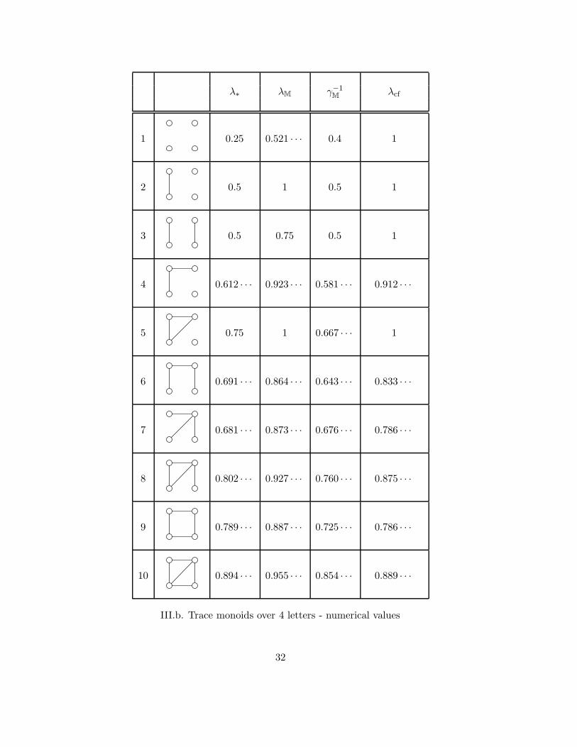
λ∗ λM γ−1M

λcf

1 0.25 0.521 · · · 0.4 1

2 0.5 1 0.5 1

3 0.5 0.75 0.5 1

4 0.612 · · · 0.923 · · · 0.581 · · · 0.912 · · ·

5 0.75 1 0.667 · · · 1

6 0.691 · · · 0.864 · · · 0.643 · · · 0.833 · · ·

7 0.681 · · · 0.873 · · · 0.676 · · · 0.786 · · ·

8 0.802 · · · 0.927 · · · 0.760 · · · 0.875 · · ·

9 0.789 · · · 0.887 · · · 0.725 · · · 0.786 · · ·

10 0.894 · · · 0.955 · · · 0.854 · · · 0.889 · · ·

III.b. Trace monoids over 4 letters - numerical values

32

Let us denote the dependence graphs in Table III, listed from top tobottom, by (Σ, Di), i = 1, . . . , 10. The graph (Σ, D9) is the cocktail partygraph CP2, hence the values of the average heights can be retrieved fromSection 6.2. More generally, most of the values in the table can be computedusing the results from the paper. The exceptions are λ∗ for (Σ, Di), i =6, 7, 8, and 10. For (Σ, D8) and (Σ, D10), the value of λ∗ can be computedby applying Proposition 12 from [5].

For (Σ, D6), the exact value of λ∗ is not known. Using truncated Markovchains, A. Jean-Marie [23] obtained the following exact bounds:

λ∗(Σ, D6) ∈ [0.69125003165, 0.69125003169] .

Let us concentrate on λ∗(Σ, D7). Let (xn)n∈N∗ be a sequence of inde-pendent random variables valued in Σ and uniformly distributed: P{xn =u} = 1/4, u ∈ Σ. Define Xn = ψ(x1 · · · xn), then (Xn)n is a Markov chainon the state space M(Σ, D7). Let a be the letter such that (a, u) ∈ D7 forall u ∈ Σ. Define T = inf{n : xn = a}. An elementary argument using theStrong Law of Large Numbers then shows that λ∗(Σ, D7) = E[h(XT )]/E[T ].It follows that

λ∗(Σ, D7) =1

4+

1

16

(∑

i∈N

1

4i

∑

i1+i2+i3=i

max(i1, i2, i3)

(i

i1, i2, i3

)). (39)

This expression involves non algebraic generalized hypergeometric series.By truncating the infinite sum and upper-bounding the remainder using theinequality max(i1, i2, i3) ≤ i1 + i2 + i3, we get the following exact bounds:

λ∗(Σ, D7) ∈ [0.6811589347, 0.6811589349] .

Another formula for λ∗(Σ, D7) involving multiple contour integrals and dueto Alain Jean-Marie is given in [5, Th. 13].

The closed form expressions for λM(Σ, D7) and γM(Σ, D7) are not givenin Table III since they are too long and do not fit. We have

λM(Σ, D7) =8(−93 − 9

√93 −

√93X + 5X2)

−1734 − 186√

93 + (141 − 5√

93)X + 67X2

X = (108 + 12√

93)1/3 , (40)

and γM(Σ, D7)−1 =

10777(529 − 23Y 2 + Y 4)(829 + 132√

62 − (139 − 6√

62)Y − 11Y 2)

3(3779 + 372√

62)(98340√

62 − 1461365 − 1529(149 + 66√

62)Y − 53885Y 2)(41)

with Y = (89 + 18√

62)1/3.

33

At last, let us comment on the value of γM for (Σ, D8). Using the resultsfrom Section 5.2, we get

γM(Σ, D8)−1 =

(1 − 2α)(4 − 5α)

7 − 27α+ 24α2, (42)

where α is the smallest root of the equation 2x3 − 8x2 + 6x − 1 = 0. Nu-merically, we have α = 0.237 · · · and γ−1

M= 0.760 · · · . In this case, Cardan’s

formulas are of no use (they provide an expression of the real α as a functionof the cubic root of a complex number).

Let us conclude by going back to the original motivation of compa-ring the degree of parallelism in different trace monoids. We claim forinstance that there is some strong evidence that (Σ, D9) is ‘more paral-lel’ than (Σ, D8). Indeed we have λ∗(Σ, D9) < λ∗(Σ, D8), λM(Σ, D9) <λM(Σ, D8), γ

−1M

(Σ, D9) < γ−1M

(Σ, D8), and λcf(Σ, D9) < λcf(Σ, D8).

Acknowledgement

The authors would like to thank Mireille Bousquet-Melou and Xavier Vi-ennot for pointing out several relevant references. We are also grateful toAlain Jean-Marie for sharing with us his knowledge on the difficult problemof computing λ∗, and to Anne Bouillard for correcting a mistake in an earlierversion of the proof of Proposition 5.1.

References

[1] J. Berstel and C. Reutenauer. Rational Series and their Languages.Springer Verlag, 1988.

[2] A. Bertoni, M. Goldwurm, and B. Palano. A fast parallel algorithm forthe speed-up problem of traces. In Proceedings of the workshop on TraceTheory and Code Parallelization, number 263-00 in Rapporto Interno,Univ. degli Studi di Milano, pages 29–36, 2000.

[3] V. Blondel, S. Gaubert, and J. Tsitsiklis. Approximating the spectralradius of sets of matrices in the max-algebra is NP-hard. IEEE Trans.Autom. Control, 45(9):1762–1765, 2000.

[4] P. Bremaud. Markov chains: Gibbs fields, Monte Carlo simulation, andqueues, volume 31 of Texts in Applied Mathematics. Springer Verlag,Berlin, 1999.

[5] M. Brilman. Evaluation de Performances d’une Classe de Systemes deRessources Partagees. PhD thesis, Univ. Joseph Fourier - Grenoble I,1996.

34

[6] M. Brilman and J.M. Vincent. On the estimation of the throughputfor a class of stochastic resources sharing systems. Mathematics ofOperations Research, 23(2):305–321, 1998.

[7] L. Carlitz. The generating function for max(n1, . . . , nk). PortugaliaeMathematica, 21(5):201–207, 1962.

[8] P. Cartier and D. Foata. Problemes combinatoires de commutation etrearrangements. Number 85 in Lecture Notes in Mathematics. SpringerVerlag, 1969.

[9] C. Cerin and A. Petit. Speedup of recognizable trace languages. InProc. MFCS 93, number 711 in Lect. Notes Comput. Sci., pages 332–341. Springer, 1993.

[10] D. Cvetkovic, M. Doob, and H. Sachs. Spectra of Graphs. Theory andApplication, volume 87 of Pure and Applied Mathematics. AcademicPress, Paris, 1980.

[11] V. Diekert and Y. Metivier. Partial commutation and traces. In Hand-book of formal languages, volume 3, pages 457–533. Springer, 1997.

[12] V. Diekert and G. Rozenberg, editors. The Book of Traces. WorldScientific, Singapour, 1995.

[13] P. Flajolet and R. Sedgewick. The average case analysis of algorithms:Complex asymptotics and generating functions. Reseach Report RR-2026, INRIA, Rocquencourt, France, 1993.

[14] S. Gaubert and J. Mairesse. Task resource models and (max,+) au-tomata. In J. Gunawardena, editor, Idempotency, volume 11, pages133–144. Cambridge University Press, 1998.

[15] S. Gaubert and J. Mairesse. Performance evaluation of timed Petri netsusing heaps of pieces. In P. Bucholz and M. Silva, editors, Petri Netsand Performance Models (PNPM’99), pages 158–169. IEEE ComputerSociety, 1999.

[16] C. Godsil. Matchings and walks in graphs. J. Graph Theory, 5:285–297,1981.

[17] C. Godsil. Algebraic Combinatorics. Chapman and Hall, 1993.

[18] C. Godsil and I. Gutman. On the theory of the matching polynomial.J. Graph Theory, 5:137–144, 1981.

[19] M. Goldwurm and M. Santini. Clique polynomials have a unique rootof smallest modulus. Information Processing Letters, 75(3):127–132,2000.

35

[20] R. Graham, D. Knuth, and O. Patashnik. Concrete mathematics: afoundation for computer science. 2nd edition. Addison-Wesley, 1994.

[21] V. Hakim and J.-P. Nadal. Exact results for 2d directed animals on astrip of finite width. J. Phys. A: Math. Gen., 16:L213–L218, 1983.

[22] A. Jean-Marie. Ers: A tool set for performance evaluation of discreteevent systems. http://www-sop.inria.fr/mistral/soft/ers.html.

[23] A. Jean-Marie. Personal communication. September 2001.

[24] D. Krob, J. Mairesse, and I. Michos. On the average parallelism in tracemonoids. In H. Alt and A. Ferreira, editors, Proceedings of STACS’02,LNCS. Springer-Verlag, 2002.

[25] J.-P. Nadal, B. Derrida, and J. Vannimenus. Directed lattice animals in2 dimensions: numerical and exact results. J. Physique, 43:1561–1574,1982.

[26] D. Revuz. Markov Chains. North-Holland Mathematical Library, 1975.

[27] N. Saheb. Concurrency measure in commutation monoids. DiscreteApplied Mathematics, 24:223–236, 1989.

[28] N. Saheb and A. Zemmari. Methods for computing the concurrencydegree of commutation monoids. In Proceedings FPSAC’00, pages 731–742, Moscow, Russia, 2000. Springer Verlag.

[29] E. Seneta. Non-negative Matrices and Markov Chains. Springer seriesin statistics. Springer Verlag, Berlin, 1981.

[30] R. Stanley. Enumerative Combinatorics, Volume I. Wadsworth &Brooks/Cole, Monterey, 1986.

[31] E.C. Titchmarsh. The Theory of Functions. 2nd ed. Oxford UniversityPress, 1975.

[32] G.X. Viennot. Heaps of pieces, I: Basic definitions and combinatoriallemmas. In Labelle and Leroux, editors, Combinatoire Enumerative,number 1234 in Lect. Notes in Math., pages 321–350. Springer, 1986.

[33] H. Wilf. Generatingfunctionology. Academic Press, 1990.

36