computing skeletons in three dimensions - image analysisingela/manuscripts/pr99_32_7_1225.pdf ·...

Pattern Recognition 32 (1999) 1225}1236

Computing skeletons in three dimensions

Gunilla Borgefors!,*, Ingela NystroK m", Gabriella Sanniti Di Baja#

!Centre for Image Analysis, Swedish University of Agricultural Sciences, SE-752 37 Uppsala, Sweden"Centre for Image Analysis, Uppsala University, SE-752 37 Uppsala, Sweden

#Istituto di Cibernetica, National Research Council of Italy, IT-800 72 Arco Felice (Napoli), Italy

Received 29 April 1997; received in revised form 18 May 1998

Abstract

Skeletonization will probably become as valuable a tool for shape analysis in 3D, as it is in 2D. We present a topologypreserving 3D skeletonization method which computes both surface and curve skeletons whose voxels are labelled withthe D6 distance to the original background. The surface skeleton preserves all shape information, so (close to) completerecovery of the object is possible. The curve skeleton preserves the general geometry of the object. No complexcomputations, large sets of masks, or extra memory are used, which make implementations e$cient. Resulting skeletonsfor geometric objects in a number of 2 Mbyte images are shown as examples. ( 1999 Pattern Recognition Society.Published by Elsevier Science Ltd. All rights reserved.

Keywords: Volume image; Shape representation; Surface skeleton; Curve skeleton; Thinning; Digital topology

1. Introduction

The history of skeletonization of digital objects is al-most as old as digital image analysis itself. The purpose isto reduce 2D discrete objects to (1D) linear representa-tions preserving topological and geometrical informa-tion. Given an input binary image, skeletonizationchanges non-skeletal object pixels into backgroundpixels. Regardless of the scheme adopted to performskeletonization, the resulting skeleton is a union ofcurves placed symmetrically with respect to the border ofthe object. The literature on 2D skeletonization is veryrich. An outline of various thinning and skeletonizationmethodologies can be found in Ref. [1].

Reducing discrete structures to lower dimensions iseven more desirable when dealing with (3D) volume

*Corresponding author. Tel.: 00 46 18 471 3466; fax: 00 46 18553 447; e-mail: [email protected]

images. The result of 3D skeletonization is either a set of3D surfaces and curves, or if even more compression isdesired, a set of only 3D curves. The compression to 3Dcurves is possible only for solid objects having no cavi-ties. A hollow torus, e.g. could never be reasonably repre-sented by a curve skeleton. The skeleton could bea promising tool for an increasing number of applica-tions, especially in biomedical imagery. However, com-pared to the literature on 2D skeletonization, the articlespublished on 3D skeletonization are still not very numer-ous. The main reason for this seems to be the di$culty toaddress and e$ciently solve essential problems, such astopology preservation, in more than two dimensions. Infact, although many concepts such as Euler character-istics, simple points and connectivity have been studiedin the past years (e.g. Refs. [2}6]), the implementation ofskeletonization methods based on their use is rathercomplicated.

The general strategy for 3D skeletonization does notdi!er signi"cantly from the strategy in the 2D case.

0031-3203/99/$20.00 ( 1999 Pattern Recognition Society. Published by Elsevier Science Ltd. All rights reserved.PII: S 0 0 3 1 - 3 2 0 3 ( 9 8 ) 0 0 0 8 2 - X

Object voxels are changed to background voxels underthe constraint that topology and geometry of the objectare preserved. However, a number of new problems haveto be solved in the 3D case. For example, when designingtopology preserving removal operations, besides preven-ting disconnections and creation of cavities, which mustbe done also in 2D, one must also avoid the creation oftunnels and the excavation of unwanted deep cavities incomplex surfaces. It seems that the geometry preservingcriteria, i.e. the de"nition of protrusions or end-points,are what separates existing algorithms; every author hashis own criteria, resulting in very di!erent skeletons.

If the skeletal voxels are labelled with their distanceto the original background and skeletonization is per-formed in a way that guarantees the inclusion in theskeleton of object voxels having locally maximal dis-tance, skeletonization becomes reversible. The object canbe recovered by applying the reverse distance trans-formation to the skeleton, see Ref. [7]. This recoveryproperty is disregarded in many approaches, but is, e.g.present in an algorithm to compute surface skeletons thatwe have recently proposed [8]. A curve skeleton cannotinclude enough information for recovery in the generalcase.

An early work on curve skeletons can be found in Ref.[9], where iterative thinning is performed based on (un-fortunately not su$cient) conditions for preservation ofthe Euler characteristics. In Ref. [10], a surface skeletonis obtained for 6-connected objects using topologicalnumbers in an algorithm using six directional sub-iter-ations. A thinning scheme based upon eight sub-"eldscan be found in Ref. [11], where (only) 26-connectivity ispreserved, either for surface or curve skeletons using thesame topological numbers. In Ref. [12], iterative erosionresulting in surface skeletons is performed on the objectborder using (rather complex) contour information. InRef. [5], simple points (removable voxels) are identi"edusing (fairly large) look-up tables, and removed in three-scan iterations. The algorithm preserves topology and isinsensitive to noise, but geometry is not fully preservedby the resulting surface skeletons. This work is continuedin Ref. [13]. In Ref. [4], the Euler characteristics arestored in look-up tables and used to identify simplepoints in a six directional sub-iterations algorithm. Theresult is either a surface or a curve skeleton depending onwhich end-point condition is used. In Ref. [14], six direc-tional sub-iterations are also used. Nice rotation inde-pendent surface or curve skeletons are obtained by usingthe Euclidean distance transform. In Ref. [15], objectsare reduced directly to 3D curves using four classes (eachwith a number) of deleting templates. The algorithm isdemonstrated on visual analysis of computer tomogra-phy lung data. In many other papers on skeletonizationof volume objects, the only examples given are tiny testimages, which makes it di$cult to understand what theresults would be for reasonably sized and/or real images.

The concept of skeletonization has also been extendedto four-dimensional data, e.g. Ref. [16], where the Eulercharacteristics are utilized, and di!erent end-point condi-tions decide the dimensionality of the skeleton.

In this paper we describe a method for thinning a vol-ume (voxel) object to a skeleton whose voxels are labelledwith the (D6) distance to the original background. Ourskeletonization method is performed in two major steps.The "rst step reduces the object to a surface skeleton(Section 3), which requires two iterative phases. Duringthe "rst phase, non-multiple voxels are iteratively re-moved until an at most two voxel thick surface of skeletalvoxels is identi"ed. During the second phase, this set isreduced to a set of one voxel thin surfaces (and curves).The original object can be recovered from its surfaceskeleton, using the distance labels. The recovery is exact ifstarted from the &&thick'' skeleton from the "rst phase,whereas some border voxels may be missing if the onevoxel thin skeleton is used. The second step reduces thesurface skeleton to a curve skeleton (Section 4), whichalso requires two phases. The skeletons are topologypreserving, but some (exceptional) objects cannot be re-duced to skeletons. We present resulting skeletons fora number of 2 Mbyte images (Section 5). The voxels ofour curve skeletons are labelled with the distance to theoriginal background. This is useful information also forthe curve skeletons, even though the original object can-not be recovered in this case.

2. De5nitions

Each voxel v has three types of neighbours among its26 closest neighbours; 6 face-, 12 edge-, and 8 point-neighbours, that share a face, an edge, and a point with v,respectively.

In a binary image we de"ne an object component asa 26-connected set of voxels. As a consequence of the26-connectedness selected for the object, 6-connectednessmust be used for the background. If the backgroundconsists of exactly one 6-connected component, then theobject is termed a solid object.

A border voxel is an object voxel with a face-neighbourin the background. Object voxels, which are not bordervoxels, are internal voxels.

Voxels are characterized by the numbers of n-connec-ted components of object or background in their neigh-bourhood. For example, a voxel is a break-point voxel if ithas more than one 26-connected object component in its26-neighbourhood. The recursive algorithm in Ref. [17]can be used to count connected components e$ciently.

Nf18 is de"ned as the number of 6-connected back-

ground components in the 18-neighbourhood of a voxelhaving the central voxel as a face-neighbour. On a 3Dsurface, an outer voxel is a surface voxel with N

f18"1. If

Nf18'1 it is called a tunnel voxel, because removing it

1226 G. Borgefors et al. / Pattern Recognition 32 (1999) 1225}1236

Fig. 1. Where two surfaces cross the outermost voxels of thecrossing are removed, but creation of deep cavities is preventedby Step 1 (ii) of the algorithm.

would create a tunnel through the object. This classi"ca-tion of surface voxels is discussed in Refs. [18] and [19].

The D6 metric is obtained by counting the number ofsteps in the minimal 6-connected path between voxels.The D6 distance is the 3D equivalent of the city-blockdistance in 2D, see Ref. [20].

The algorithm in this paper is partly parallel in nature,partly sequential. Operations performed in parallel areparallel in the sense that the local operations are parallel,i.e. all voxels can and should be processed simultaneouslyin each iteration. In sequential operations, neighbouringvoxels cannot be processed simultaneously. Our methodis implemented on standard sequential computers, usingpseudo-parallel programs.

3. Surface skeletonization

The algorithm described in the following is an im-proved version of the one presented in Ref. [8].

3.1. Identixcation of removable voxels

Voxels are iteratively removed from the object, untilno more voxels can be removed. Each iterationconsists of four steps (or scans through the image). Everystep can be performed in parallel.

Step 1:(1) Among voxels not already labelled, identify border

voxels, and label them with the current iterationnumber.

(2) Among internal voxels, identify voxels with an edge-neighbour in the background and label them with thecurrent iteration number plus one.Step 2: Among voxels labelled with the current iter-ation number, mark those that are multiple.Step 3: Among non-multiple voxels labelled with thecurrent iteration number, mark as tunnel voxelsthose for which N

f18'1. When computing

Nf18'1 neighbouring non-multiple voxels labelled

with the current iteration number are interpreted asbackground voxels, i.e. they are treated as if they werealready removed.Step 4: Remove all unmarked border voxels.

The process terminates when all border voxels are mul-tiple, and hence no more voxels can be removed.

During Step 1 border voxels in all directions are simul-taneously identi"ed, in contrast to some earlier parallelthinning work, e.g. Refs. [4,10], where each iteration isdivided into six directional sub-iterations. That direc-tional strategy is a generalization of the 2D case, but itmay cause topological problems in 3D, such as discon-necting objects.

Since only border voxels are candidates for removal,cavities are not created. Labelling the voxels with anedge-neighbour in the background with the iterationnumber plus one, gives them the correct distance label(from the original background). This is important forobject recovery, and guarantees that Step 2 will be per-formed on all voxels with the same distance in the sameiteration. An illustrative example is shown using twocrossing planes, see Fig. 1. Consider the internal voxelsplaced at the intersection of the planes, and suppose thatwe do not label them as requested by Step 1 (ii). Removalof the border voxels in the intersection, exposes to thebackground other voxels in the intersection. These voxelswould become removable in the next iteration. By iterat-ing this removal, the surface skeleton would "nally havefour planes linked to each other only by a single middlevoxel. This would still be topologically correct, but notvery geometry preserving. If we instead consider that allvoxels in the intersection would have the same distancelabel in the D6 distance transform of the object, it be-comes apparent that they should all be checked for re-moval in the same iteration. Labelling the voxels with anedge-neighbour in the background as in Step 1 (ii) pre-vents creation of deep, narrow cavities where two surfa-ces intersect. Consequently, only the outermost voxels ofthe crossings are removed.

In Step 2 we identify multiple voxels in a way that isa generalization of a 2D algorithm that identi"es themultiple pixels on the border of an 8-connected object,see Ref. [21]. Multiple pixels have been proved to beequivalent to pixels that can not be removed duringskeletonization, see Ref. [22]. The resulting skeletalpixels are labelled as they would be in the city-blockdistance transform of the object. Moreover, it can beshown that the multiple pixels include all the pixels thatare local maxima of the city-block distance transform.

For volume images, we de"ne a border voxel of thecurrent iteration, v, as multiple if any of ConditionsA1}A3 is satis"ed:

Condition A1: No pair of opposite face-neighbours (alig-ned along one of the three principal planes) of v exists

G. Borgefors et al. / Pattern Recognition 32 (1999) 1225}1236 1227

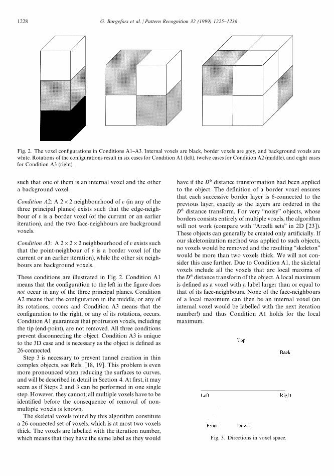
Fig. 2. The voxel con"gurations in Conditions A1}A3. Internal voxels are black, border voxels are grey, and background voxels arewhite. Rotations of the con"gurations result in six cases for Condition A1 (left), twelve cases for Condition A2 (middle), and eight casesfor Condition A3 (right).

Fig. 3. Directions in voxel space.

such that one of them is an internal voxel and the othera background voxel.

Condition A2: A 2]2 neighbourhood of v (in any of thethree principal planes) exists such that the edge-neigh-bour of v is a border voxel (of the current or an earlieriteration), and the two face-neighbours are backgroundvoxels.

Condition A3: A 2]2]2 neighbourhood of v exists suchthat the point-neighbour of v is a border voxel (of thecurrent or an earlier iteration), while the other six neigh-bours are background voxels.

These conditions are illustrated in Fig. 2. Condition A1means that the con"guration to the left in the "gure doesnot occur in any of the three principal planes. ConditionA2 means that the con"guration in the middle, or any ofits rotations, occurs and Condition A3 means that thecon"guration to the right, or any of its rotations, occurs.Condition A1 guarantees that protrusion voxels, includingthe tip (end-point), are not removed. All three conditionsprevent disconnecting the object. Condition A3 is uniqueto the 3D case and is necessary as the object is de"ned as26-connected.

Step 3 is necessary to prevent tunnel creation in thincomplex objects, see Refs. [18, 19]. This problem is evenmore pronounced when reducing the surfaces to curves,and will be described in detail in Section 4. At "rst, it mayseem as if Steps 2 and 3 can be performed in one singlestep. However, they cannot; all multiple voxels have to beidenti"ed before the consequence of removal of non-multiple voxels is known.

The skeletal voxels found by this algorithm constitutea 26-connected set of voxels, which is at most two voxelsthick. The voxels are labelled with the iteration number,which means that they have the same label as they would

have if the D6 distance transformation had been appliedto the object. The de"nition of a border voxel ensuresthat each successive border layer is 6-connected to theprevious layer, exactly as the layers are ordered in theD6 distance transform. For very &&noisy'' objects, whoseborders consists entirely of multiple voxels, the algorithmwill not work (compare with &&Arcelli sets'' in 2D [23]).These objects can generally be created only arti"cially. Ifour skeletonization method was applied to such objects,no voxels would be removed and the resulting &&skeleton''would be more than two voxels thick. We will not con-sider this case further. Due to Condition A1, the skeletalvoxels include all the voxels that are local maxima ofthe D6 distance transform of the object. A local maximumis de"ned as a voxel with a label larger than or equal tothat of its face-neighbours. None of the face-neighboursof a local maximum can then be an internal voxel (aninternal voxel would be labelled with the next iterationnumber!) and thus Condition A1 holds for the localmaximum.


Fig. 4. Four-voxels con"guration for removing Top-voxels (seetext). Border voxels are grey, background voxels are white.

Fig. 5. A voxel set, two voxels thick in the Front}Back direc-tion. The Top-voxels (hatched) are not removed in theTop}Down process, but the horizontally hatched Top-voxelsare also Front-voxels and will be removed during the Front-Back process.

A few internal voxels might still remain after this "rstthinning in regions where many surfaces and/or curvesmeet (due to the fact that remaining object voxels haveformed &&Arcelli sets''). It is even conceivable that thesevoxels are not yet labelled, i.e. they do not have anedge-neighbour in the background. Such voxels shouldbe assigned a label equal to the minimum label in their6-neighbourhood plus one, which corresponds to thevalue they would have in the D6 distance transform.

As local maxima are not removed, object recovery ispossible, using the reverse D6 distance transformation,see Ref. [7]. The pseudo-code for the forward pass isgiven below. The backward pass is similar, but scansthrough the image in the opposite direction.

/*}}}}}}}}}}FORWARD PASS}}}}}}}}}}}*/

LOOP}X}Y}Z (image) M

if (x(xLOEx'xHIEy(yLOEy'yHIEz(zLOEz'zHI)

image"0; /* image border omitted */elseimage"MAX( I(x, y, z!1)!1,

I(x, y!1, z)!1,I(x!1, y, z)!1,I )

N/*}}}}}}END}}FORWARD PASS}}}}}}}}}*/

3.2. Thinning to unit-wide surface skeleton

The skeletal set obtained is at most two voxels thick. Itcan be reduced to unit thickness by applying a thinningprocess that has to be split into six directional processes,each of them applied once. Using directional processes isnecessary to prevent breaking connectedness and excess-ive shortening.

The six processes occur sequentially in the directionsTop}Down, Down}Top, Left}Right, Right}Left,Front}Back, and Back}Front, see Fig. 3. A Top-voxel isde"ned as a skeletal voxel with a background voxel as theface-neighbour in the Top-direction. The other "ve aresimilarly de"ned.

In the Top}Down process Top-voxels are candidatesfor sequential removal. A Top-voxel v is removed if allConditions B1}B3 are satis"ed:

Condition B1: The face-neighbour of v in the Down-direction is a Down-voxel. See Fig. 4.

Condition B2: Condition A2 does not occur.Condition B3: Condition A3 does not occur.

Condition B1 guarantees that the current Top}voxelbelongs to a portion of the set of the skeletal voxels whichis exactly two voxels thick in the Top-Down direction.For example, see Fig. 5, illustrating a set that is twovoxels thick in the Front}Back direction. The Top-voxelsof the set do not satisfy Condition B1, so they are not

removed during the Top}Down process, thus, unwanted&&shrinking'' of the set is prevented in the Top}Downdirection.

Condition B2 prevents breaking the connectedness ofthe set when the connection occurs between edge-neigh-bours only. Only four of the twelve rotational cases ofCondition A2 (see middle of Fig. 2) have to be checked,as Condition B1 guarantees connection in the other


Fig. 6. A thin surface where the outer voxels are marked in grey.The hatched voxels are erroneously identi"ed as outer voxels, ifcounting the 6-connected background components in the 26-neighbourhood; the 18-neighbourhood should used.

Fig. 7. A 26-neighbourhood shown slice with a &&cap'' in theFront-direction. The central voxel is a tip-of-protection voxel.Background voxels are white. &&Don't care'' voxels are grey.Rotation of the &&cap'' gives the other "ve direction masks.

Fig. 8. A box (left), its surface skeleton of labelled voxels (middle), and its curve skeleton (right).

cases. The cases to be checked are those where the edge-neighbour connects to one of the four upper edges of thevoxel.

Condition B3 prevents breaking the connectedness ofthe set when the connection occurs between point-neigh-bours only. As Condition B1 guarantees connection infour cases, Condition A3 has to be checked only for thecases where the point-neighbour connects to one of thefour upper corners of the voxel (see right of Fig. 2).

The other "ve processes are similar. After the six direc-tional processes have been applied, the skeleton consistsof thin surfaces and curves. Some of the local maxima ofthe implied distance transform could have been removedduring this thinning process, so complete object recoveryby the reverse distance transformation is no longer pos-sible. However, the voxels that are not recovered are allborder voxels of the original object, so the distortion ofobject shape is not great.

4. Curve skeletonization

The surface skeleton can be further reduced to a curveskeleton. The original object cannot thereafter be re-

covered, but its topology and geometry are preserved.The skeletal voxels are labelled with their (D6) distance tothe original background, which might be useful informa-tion in quantitative analysis of the shape.

4.1. Identixcation of removable voxels

Voxels are iteratively removed from the surface, untilno more voxels can be removed. Each iteration consistsof three steps (or scans through the image). Di!erentlyfrom before, only the two "rst steps are performed inparallel.

Step 1: Identify outer voxels, Nf18"1, on the surface.

Step 2: Inspect all outer voxels (both from the currentand earlier iterations). Mark a voxel as removable, if it


Fig. 9. Top: A pyramid (left), its surface skeleton (middle), and its curve skeleton (right). Bottom: The pyramid rotated 453 (left), itssurface skeleton (middle), and its curve skeleton (right).

Fig. 10. A cylinder (left), its surface skeleton (middle), and its curve skeleton (right).

has two 26-connected components of outer voxels, butonly one 26-connected component of object in its 26-neighbourhood.

Step 3: Sequentially remove marked voxels, unlessthey are break-point voxels.

During Step 1 the voxels which are candidates forremoval, the outer voxels, are identi"ed. Intuitively, in-terior surface voxels have more than one backgroundcomponent in their neighbourhood, and voxels on theborder of a surface have one background component. Asthe background is 6-connected, its components arecounted using 6-connectedness. In Fig. 6 the outer voxelsof a surface are marked in grey. When counting compo-nents in the 26-neighbourhood, the hatched voxels are

also identi"ed as outer voxels, as the background isconnected through the point-neighbours of these voxels.Removal of a hatched voxel would change the topologyof the object as a tunnel would be created, therefore theymust not be identi"ed as outer voxels. A 3D surface isactually 18-connected, therefore the 18-neighbourhoodshould be used when counting background components.Simply counting components in the 18-neighbourhoodwill not however, identify all removable voxels. For somecomplex surfaces the number of background componentsfor removable border voxels are more than one, as back-ground voxels being edge-connected to the central voxelare included as components (of size one voxel). Thesolution is to count only the 6-connected background


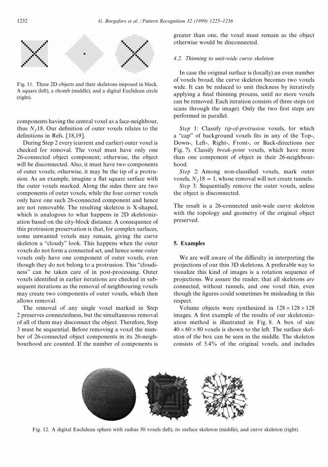
Fig. 11. Three 2D objects and their skeletons imposed in black.A square (left), a rhomb (middle), and a digital Euclidean circle(right).

Fig. 12. A digital Euclidean sphere with radius 50 voxels (left), its surface skeleton (middle), and curve skeleton (right).

components having the central voxel as a face-neighbour,thus N

f18. Our de"nition of outer voxels relates to the

de"nitions in Refs. [18,19].During Step 2 every (current and earlier) outer voxel is

checked for removal. The voxel must have only one26-connected object component; otherwise, the objectwill be disconnected. Also, it must have two componentsof outer voxels; otherwise, it may be the tip of a protru-sion. As an example, imagine a #at square surface withthe outer voxels marked. Along the sides there are twocomponents of outer voxels, while the four corner voxelsonly have one such 26-connected component and henceare not removable. The resulting skeleton is X-shaped,which is analogous to what happens in 2D skeletoniz-ation based on the city-block distance. A consequence ofthis protrusion preservation is that, for complex surfaces,some unwanted voxels may remain, giving the curveskeleton a &&cloudy'' look. This happens when the outervoxels do not form a connected set, and hence some outervoxels only have one component of outer voxels, eventhough they do not belong to a protrusion. This &&cloudi-ness'' can be taken care of in post-processing. Outervoxels identi"ed in earlier iterations are checked in sub-sequent iterations as the removal of neighbouring voxelsmay create two components of outer voxels, which thenallows removal.

The removal of any single voxel marked in Step2 preserves connectedness, but the simultaneous removalof all of them may disconnect the object. Therefore, Step3 must be sequential. Before removing a voxel the num-ber of 26-connected object components in its 26-neigh-bourhood are counted. If the number of components is

greater than one, the voxel must remain as the objectotherwise would be disconnected.

4.2. Thinning to unit-wide curve skeleton

In case the original surface is (locally) an even numberof voxels broad, the curve skeleton becomes two voxelswide. It can be reduced to unit thickness by iterativelyapplying a "nal thinning process, until no more voxelscan be removed. Each iteration consists of three steps (orscans through the image). Only the two "rst steps areperformed in parallel.

Step 1: Classify tip-of-protrusion voxels, for whicha &&cap'' of background voxels "ts in any of the Top-,Down-, Left-, Right-, Front-, or Back-directions (seeFig. 7). Classify break-point voxels, which have morethan one component of object in their 26-neighbour-hood.

Step 2: Among non-classi"ed voxels, mark outervoxels, N

f18"1, whose removal will not create tunnels.

Step 3: Sequentially remove the outer voxels, unlessthe object is disconnected.

The result is a 26-connected unit-wide curve skeletonwith the topology and geometry of the original objectpreserved.

5. Examples

We are well aware of the di$culty in interpreting theprojections of our thin 3D skeletons. A preferable way tovisualize this kind of images is a rotation sequence ofprojections. We assure the reader, that all skeletons areconnected, without tunnels, and one voxel thin, eventhough the "gures could sometimes be misleading in thisrespect.

Volume objects were synthesized in 128]128]128images. A "rst example of the results of our skeletoniz-ation method is illustrated in Fig. 8. A box of size40]60]80 voxels is shown to the left. The surface skel-eton of the box can be seen in the middle. The skeletonconsists of 5.4% of the original voxels, and includes


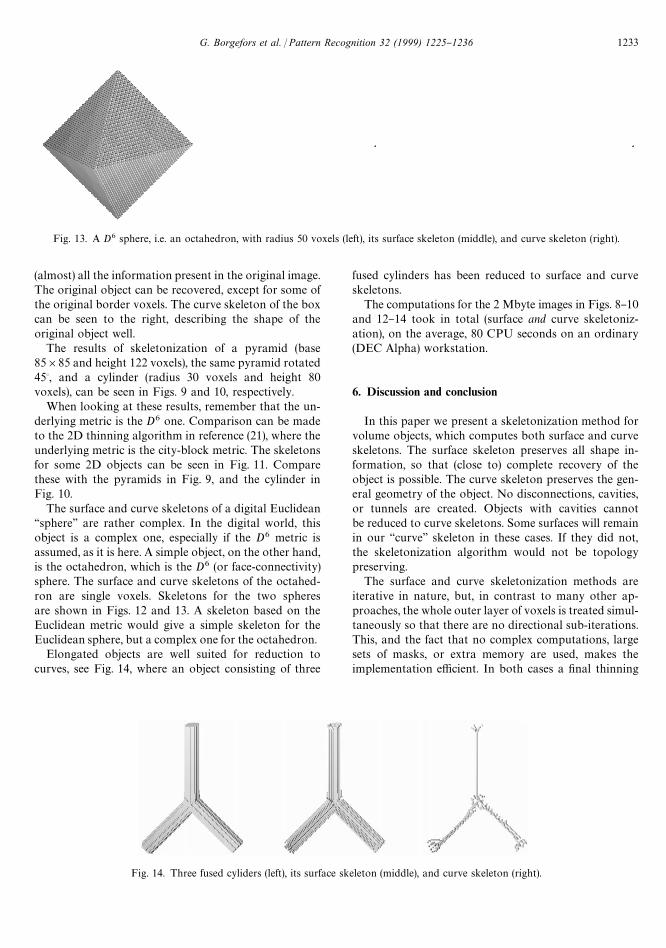
Fig. 13. A D6 sphere, i.e. an octahedron, with radius 50 voxels (left), its surface skeleton (middle), and curve skeleton (right).

Fig. 14. Three fused cyliders (left), its surface skeleton (middle), and curve skeleton (right).

(almost) all the information present in the original image.The original object can be recovered, except for some ofthe original border voxels. The curve skeleton of the boxcan be seen to the right, describing the shape of theoriginal object well.

The results of skeletonization of a pyramid (base85]85 and height 122 voxels), the same pyramid rotated45", and a cylinder (radius 30 voxels and height 80voxels), can be seen in Figs. 9 and 10, respectively.

When looking at these results, remember that the un-derlying metric is the D6 one. Comparison can be madeto the 2D thinning algorithm in reference (21), where theunderlying metric is the city-block metric. The skeletonsfor some 2D objects can be seen in Fig. 11. Comparethese with the pyramids in Fig. 9, and the cylinder inFig. 10.

The surface and curve skeletons of a digital Euclidean&&sphere'' are rather complex. In the digital world, thisobject is a complex one, especially if the D6 metric isassumed, as it is here. A simple object, on the other hand,is the octahedron, which is the D6 (or face-connectivity)sphere. The surface and curve skeletons of the octahed-ron are single voxels. Skeletons for the two spheresare shown in Figs. 12 and 13. A skeleton based on theEuclidean metric would give a simple skeleton for theEuclidean sphere, but a complex one for the octahedron.

Elongated objects are well suited for reduction tocurves, see Fig. 14, where an object consisting of three

fused cylinders has been reduced to surface and curveskeletons.

The computations for the 2 Mbyte images in Figs. 8}10and 12}14 took in total (surface and curve skeletoniz-ation), on the average, 80 CPU seconds on an ordinary(DEC Alpha) workstation.

6. Discussion and conclusion

In this paper we present a skeletonization method forvolume objects, which computes both surface and curveskeletons. The surface skeleton preserves all shape in-formation, so that (close to) complete recovery of theobject is possible. The curve skeleton preserves the gen-eral geometry of the object. No disconnections, cavities,or tunnels are created. Objects with cavities cannotbe reduced to curve skeletons. Some surfaces will remainin our &&curve'' skeleton in these cases. If they did not,the skeletonization algorithm would not be topologypreserving.

The surface and curve skeletonization methods areiterative in nature, but, in contrast to many other ap-proaches, the whole outer layer of voxels is treated simul-taneously so that there are no directional sub-iterations.This, and the fact that no complex computations, largesets of masks, or extra memory are used, makes theimplementation e$cient. In both cases a "nal thinning


step is necessary, as the "rst skeleton will be two voxelsthick where the original object has even thickness.

As the underlying metric used in the skeletonization isD6, the skeletons produced su!ers from the same weak-ness as the skeletonization based on the city-block metricin 2D (see Ref. [20]); the skeletons are not rotationindependent, as illustrated by the synthetic object inFig. 9. Objects in real application images do not accentu-ate the problem like this, though. Real objects are notlikely to be smooth, and, hence, the skeletons are com-plex. Their extra or missing skeleton branches due torotation can often be disregarded. The rotation depend-endcy problem can be alleviated by a pre-processing step,where the object is rotated into a &&normalized'' position,for example, by placing the maximum diameter alongone coordinate axis, the maximum thickness orthogonalto this axis as another coordinate axis, and "nally theaxis orthogonal to these two as the third coordinate axis,see Ref. [24]. In this way, similar structures will alwaysget the same normalized orientation. A future solution isto develop skeletons based on more rotation-indepen-dent underlying metrics. Our skeletonization can be seenas the starting point to understand how skeletons can beextracted from any distance map.

Every protrusion that is not (locally) a corner of anoctahedron will generate a skeletal branch, i.e., skeleton-ization is sensitive to noise. Pre-processing in the form ofmorphological smoothing operations will alleviate (butnot solve) this problem, especially if a small octahedron isused as a structuring element. A simple way to implementsmoothing in our algorithm, is to apply unconditionedremoval for a number of iterations proportional to theexpected noise size (with the drawback that signi"cantskeleton branches are correspondingly shortened). Real-istically, however, skeletons from real applicationsshould be pruned as both signi"cant and unwanted skel-etal branches will be present in our skeletons. Hence, thepruning task is to identify and remove the unwantedbranches. Methods with pruning built into the iterativethinning process might not be able to distinguish be-tween unwanted and signi"cant branches, when not us-ing information from the total skeleton, and thereforeremove some signi"cant branches. Developing goodpruning strategies for 3D surface and curve skeletons isan important problem for further research. As for theskeletonization itself, the pruning can be expected to besigni"cantly more complex than in 2D.

Because of the underlying metric, objects with #atsurfaces will produce much &&nicer'' skeletons than objectswith curved surfaces (cf. Figs. 8 and 12). The only way tosolve this is to develop skeletons based on more rotationindependent underlying metrics.

Skeletonization has proved to be a valuable tool forshape analysis in 2D. We have no doubt that it willeventually prove so also in 3D. So far, the major part ofvolume images have been representations of various parts

of the human body. Skeletonization of di!erent organswithin the body will make manipulation and analysis oftheir shape easier. For compact objects, such as the kid-neys or liver, surface skeletonization is suitable. For tube-like objects, such as blood vessels and trachea, curveskeletonization preserves the essential information, espe-cially since the curve voxels are marked with the currentdiameter of the tube. Various 3D imaging techniques arebecoming more and more available, and so are the neces-sary memory and computing power to handle these im-ages. This means that many new applications will appear.Production quality control, both in macro and microscales, for industrial products (e.g. paper, cloth, and ma-chine parts), animal, and vegetable &&objects'' and tissues(e.g. fruit, seed, and cell structure), comes to mind.

7. Summary-computing skeletons in three dimensions

Skeletonization of (3D) volume objects denotes eitherreduction to a 2D structure of 3D surfaces and curves, or,if even more compression is desired and the object to beskeletonized has no cavities, reduction to a 1D structureof only 3D curves. The general strategy for 3D skeleton-ization doet not di!er signi"cantly from the strategy inthe 2D case. Object voxels are changed to backgroundvoxels under the constraint that geometry of the objectand topology are preserved.

In this paper we present a topology preserving skel-etoniztion method for volume objects, which computesboth surface and curve skeletons. The surface skeletonpreserves all shape information, so that (close to) com-plete recovery of the object is possible. The curve skel-eton preserves the general geometry of the object. Voxelsof our skeletons are labelled with the D6 distance to theoriginal background. This is useful information not onlyfor the surface skeleton where it enables object recovery,but also for the curve skeletons, even though the originalobject cannot be recovered in this case. No discon-nections cavities or tunnels are created.

Our skeletonization method is performed in two majorsteps. The "rst step reduces the object to a surface skel-eton, which requires two iterative phases. During the "rstpase, non-multiple voxels are iteratively removed until anat most two voxel thick surface of skeletal voxels isidenti"ed. During the second phase, this set is reduced toa set of one voxel thick surfaces (and curves). The originalobject can be recovered from its surface skeleton, usingthe distance labels. The second step reduces the surfaceskeleton, to a curve skeleton, which also requires twophases. The "rst reduces the surfaces to curves, the sec-ond thins the curves to one voxel thickness. We presentresulting skeletons for a number of synthetic and real2 Mbyte images.

The surface and curve skeletonization methods areiterative in nature, but, in contrast to many other


approaches, the whole outer layer of voxels is treatedsimultaneously, so that there are no directional sub-iterations. This, and the fact that no complex computa-tions or extra memory are used, makes the implementa-tions e$cient, even on an standard sequentialworkstation, where, on the average, 80 CPU seconds areenough to skeletonize objects in 2 Mbyte images.

Skeletonization has proved to be a valuable toolfor shape analysis in 2D. We have no doubt that itwill eventually prove so also in 3D. So far, the majorpart of volume images have been representations ofvarious parts of the human body, but many new ap-plications will appear with the increase in computercapacity. Production quality control, both in macro andmicro scales, for industrial products (e.g. paper,cloth, and machine parts), animal and vegetable &&objects''and tissues (e.g. fruit, seed, and cell structure), comes tomind.

Acknowledgements

Scienti"c support were given by Prof. Ewert Bengtssonand Dr. Bo Nordin, which is gratefully acknowledged, asis the "nancial support of the Swedish Research Councilfor Engineering Science (TFR), grant number 95}182.

References

[1] L. Lam, S.-W. Lee, C.Y. Suen, Thinning methodologies }a comprehensive survey, IEEE Trans. Pattern Anal. Mach.Intell. 14 (9) (1992) 869}885.

[2] T.Y. Kong, A. Rosenfeld, Digital topology: intro-duction and survey, Comput. Vision, Graphics, ImageProcess. 48 (1989) 357}393.

[3] G. Bertrand, Simple points, topological numbers andgeodesic neighbourhoods in cubic grids, Pattern Recogni-tion Lett. 15 (1994) 1003}1011.

[4] T.-C. Lee, R.L. Kashyap, C-N. Chu, Building skeletonmodels via 3-D medial surface/axis thinning algorithms,CVGIP: Graphical Models Image Process. 56 (6) (1994)462}478.

[5] P.K. Saha, B.B. Chaudhuri. Detection of 3-D simple pointsfor topology preserving transformations with applicationto thinning, IEEE Trans. on Pattern Anal. Mach. Intell. 16(10) (1994) 1028}1032.

[6] T.Y. Kong, On topology preservation in 2-D and 3-Dthinning, Int. J. Pattern Recognition Arti"cial Intell. 9 (5)(1995) 813}844.

[7] I. NystroK m, G. Borgefors. Synthesising objects and scenesusing the reverse distance transformation in 2D and 3D, in:C. Braccini, L. DeFloriani, G. Vernazza, (Eds.), Proceed-ings of ICIAP'95: Image Analysis and Processing, Spring-er, Berlin, 1995, pp. 441}446.

[8] G. Borgefors, I. NystroK m, G.S. di Baja, Surface skeletoniz-ation of volume objects, in: P. Perner, P. Wang, and A.Rosenfeld (Eds.), Proceedings of SSPR'96: Advances inStructural and Syntactical Pattern Recognition, Springer,Berlin, Heidelberg, 1996, pp. 251}259.

[9] S. Lobregt, P.W. Verbeek, F.C.A. Groen, Three-dimen-sional skeletonization: principle and algorithm, IEEETrans. Pattern Anal. Mach. Intell. PAMI-2 (1) (1980) 75}77.

[10] G. Bertrand, A parallel thinning algorithm for medialsurfaces, Pattern Recognition Lett. 16 (1995) 979}986.

[11] G. Bertrand, Z. Aktouf, A three-dimensional thinningalgorithm using sub"elds, in: R.A. Melter, A.Y. Wu (Eds.),Vision Geometry III, Proc. SPIE 2356, 1994, pp. 113}124.

[12] S. Miguet, V. Marion-Poty, A new 2-D and 3-D thinningalgorithm based on successive border generations, Proc.4th Conf. on Discrete Geometry in Computer Imagery,Grenoble, France, 1994, pp. 195}206.

[13] P.K. Saha, D.D. Majumder, A topology and shapepreserving thinning and segmentation method for 3Ddigital space, Image Process. Commun. 2 (3) (1997) 3}34.

[14] T. Saito, J.I. Toriwaki, A sequential thinning algorithm forthree dimensional digital pictures using the Euclidean dis-tance transformation, Proc. 9th Scand. Conf. on ImageAnalysis, Uppsala, Sweden, 1995, pp. 507}51.

[15] Cherng Min Ma, M. Sonka, A fully parallel 3D thinningalgorithm and its applications. Computer Vision ImageUnderstanding, 64 (3) (1996) 420}433.

[16] P.P. Jonker, O. Vermeij, On skeletonization in 4D images,in: P. Perner, P. Wang, A. Rosenfeld (Eds.), Proc. SSPR'96:Advances in Structural and Syntactical Pattern Recogni-tion, Springer, Berlin, Heidelberg, 1996, pp. 79}89.

[17] G. Borgefors, I. NystroK m, G.S. di Baja, Connected compo-nents in 3D neighbourhoods, Proc. 10th Scand. Conf. onImage Analysis, Lappeenranta, Finland, 1997, pp.567}572.

[18] G. Malandain, G. Bertrand, N. Ayache, Topologicalsegmentation of discrete surfaces, Int. J. Comput. Vision10 (2) (1993) 183}197.

[19] P.K. Saha, B.B. Chaudhuri, 3D digital topology underbinary transformation with applications, Comput. VisionImage Understanding 63 (3) (1996) 418}429.

[20] G. Borgefors, On digital distance transforms in three di-mensions, Comput. Vision Image Understanding 64 (3)(1996) 368}376.

[21] C. Arcelli, G.S. di Baja. A one- pass two-operations processto detect the skeletal pixels on the 4-distance transform,IEEE Trans. Pattern Anal. Mac. Intell. 11 (4) (1989)411}414.

[22] C. Arcelli, G.S. di Baja, A contour characterizationfor multiply connected "gures, Pattern Recognition Lett.,6 (1987) 245}249.

[23] C. Arcelli. Pattern thinning by contour tracing, Comput.Graphics Image Process. 17 (1981) 130}144.

[24] I. NystroK m, E. Bengtsson, B. Nordin, G. Borgefors,Quantitative analysis of volume images } electron micro-scopic tomography of HIV, Medical Imaging 1994: ImageProcessing, Proc. SPIE 2167, 1994, pp. 296}303.


About the Author*GUNILLA BORGEFORS received the M. Eng. and Lic. Eng. in Applied Mathematics, from LinkoK ping Universityin 1975 and 1983, respectively; her Ph.D. in Numerical Analysis, from the Royal Institute of Technology, Stockholm in 1986; and her&&Docent'' in Image Processing from LinkoK ping University in 1992, all in Sweden. From 1982 to 1993 she was employed at the NationalDefence Research Establishment, LinkoK ping, Sweden, eventually as Director of Research for computer vision, and in 1990}1993 as Headof the Division of Information Systems. From 1993 she is full Professor at Centre for Image Analysis, Swedish University of AgriculuralSciences,Uppsala, Sweden. Borgefors was President of the Swedish Society for Automated Image Analysis in 1988}1992 and Secretaryand 1st Vice President of the International Association for Pattern Recognition, in 1990}1994 and 1994}96, respectively. Borgefors haspublished a large number of papers in international journals and conferences, and has been the editor of three books on image analysis.Her current research interests are digital geometry in two, three and higher dimensions and the application of image analysis in remotesensing and in industry.

About the Author*INGELA NYSTROG M received the M.Sc., degree in Applied Computer Science and Mathematics, and the Ph.D.degree in Computerized Image Analysis from Uppsala University, Sweden, in 1991, and in 1997, respectively. She is currentlya Researcher and Lecturer at the Centre for Image Analysis, Uppsala, Sweden. Her research interest is method development forqualitative shape analysis of volume objects.

About the Author*GABRIELLA SANNITI Di Baja received the Doctoral degree in Physics from the University of Naples, Naples,Italy, in 1973. Since then, she has been working in the "eld of Image Processing and Pattern Recognition at the Istituto di Cibernetica ofthe National Research Council of Italy, Naples, where she currently has the position of Director of Research. Sanniti di Baja haspublished more than one hundred papers in international journals and conference proceedings, and has been editor of four books. Hermain research activities concern two-dimensional shape representation, decomposition and description. Sanniti di Baja is one of theorganizers of the International Workshop on Visual Form. She has been chairman of the Education Committee of the InternationalAssociation for Pattern Recognition (IAPR) 1991}1994. Since October 1994, she is the IAPR Secretary.


computing skeletons in three dimensions - image analysisingela/manuscripts/pr99_32_7_1225.pdf ·...

Documents