computing determinants with gauss-jordan operations
TRANSCRIPT

Computing Determinants withGauss-Jordan Operations
Gene Quinn (from Carlos Curley’s notes)
Computing Determinants with Gauss-Jordan Operations – p.1/34

Computing DeterminantsWe have previously developed a formula for thedeterminant of a 2 × 2 matrix,
det(A) = det
[
a b
c d
]
= ad − bc
Computing Determinants with Gauss-Jordan Operations – p.2/34
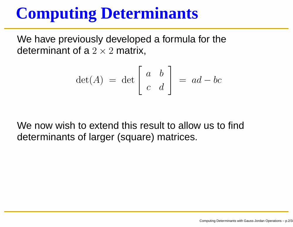
Computing DeterminantsWe have previously developed a formula for thedeterminant of a 2 × 2 matrix,
det(A) = det
[
a b
c d
]
= ad − bc
We now wish to extend this result to allow us to finddeterminants of larger (square) matrices.
Computing Determinants with Gauss-Jordan Operations – p.2/34

Computing DeterminantsWe proved the following properties for determinants of 2 × 2matrices:
det(I2) = 1
If A is upper triangular (or diagonal, or lower triangular),det(A) is the product of the diagonal elements of A.
Adding a multiple of one row of A to another leavesdet(A) unchanged
Interchanging two rows changes the sign of det(A)
Multiplying a row of A by a constant k multiplies det(A)by k.
Computing Determinants with Gauss-Jordan Operations – p.3/34

Computing DeterminantsWe proved the following properties for determinants of 2 × 2matrices:
det(I2) = 1
If A is upper triangular (or diagonal, or lower triangular),det(A) is the product of the diagonal elements of A.
Adding a multiple of one row of A to another leavesdet(A) unchanged
Interchanging two rows changes the sign of det(A)
Multiplying a row of A by a constant k multiplies det(A)by k.
We also noted (without proof) that these properties hold forn × n matrices, n = 2, 3, . . ..
Computing Determinants with Gauss-Jordan Operations – p.3/34

Computing DeterminantsAssuming the five properties from the previous slide holdfor n × n matrices, we can develop a method of computingthe determinant for any square matrix.
The method will be based on Gauss-Jordan or rowoperations.
Computing Determinants with Gauss-Jordan Operations – p.4/34
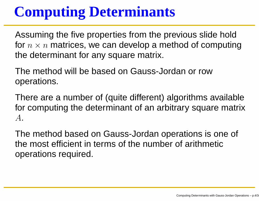
Computing DeterminantsAssuming the five properties from the previous slide holdfor n × n matrices, we can develop a method of computingthe determinant for any square matrix.
The method will be based on Gauss-Jordan or rowoperations.
There are a number of (quite different) algorithms availablefor computing the determinant of an arbitrary square matrixA.
The method based on Gauss-Jordan operations is one ofthe most efficient in terms of the number of arithmeticoperations required.
Computing Determinants with Gauss-Jordan Operations – p.4/34

Computing DeterminantsIn outline form, the method is:
Start with a square matrix A
If necessary, perform row operations to transform it toan upper triangular matrix
Keep track of each row operation and its effect on thedeterminant of the matrix
When an upper triangular matrix is obtained, computeits determinant as the product of its diagonal entries
Use the record of the changes to the determinant fromthe row operations to work backwards to thedeterminant of the original matrix A.
Computing Determinants with Gauss-Jordan Operations – p.5/34

Elementary MatricesRecall that the Gauss-Jordan reduction transforms a matrixA to rref(A) by a series of operations on the rows of A.
Computing Determinants with Gauss-Jordan Operations – p.6/34

Elementary MatricesRecall that the Gauss-Jordan reduction transforms a matrixA to rref(A) by a series of operations on the rows of A.
Each operation consists of one of the following kinds of rowoperations:
Add a multiple of one row to another row
Multiply a row by some constant k
Interchange two rows
Although we considered them purely algebraic operations,in fact each of them is equivalent to multiplication of A onthe left by a matrix.
Computing Determinants with Gauss-Jordan Operations – p.6/34
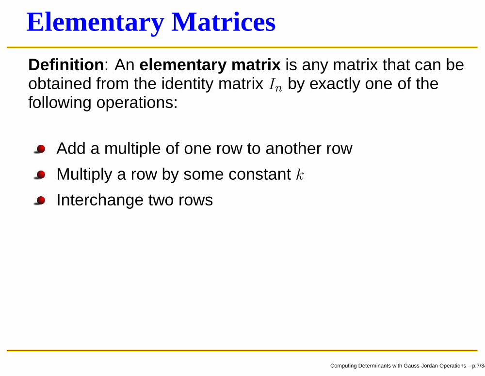
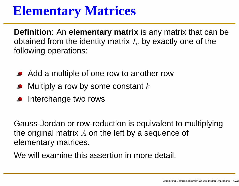
Elementary MatricesDefinition : An elementary matrix is any matrix that can beobtained from the identity matrix In by exactly one of thefollowing operations:
Add a multiple of one row to another row
Multiply a row by some constant k
Interchange two rows
Computing Determinants with Gauss-Jordan Operations – p.7/34
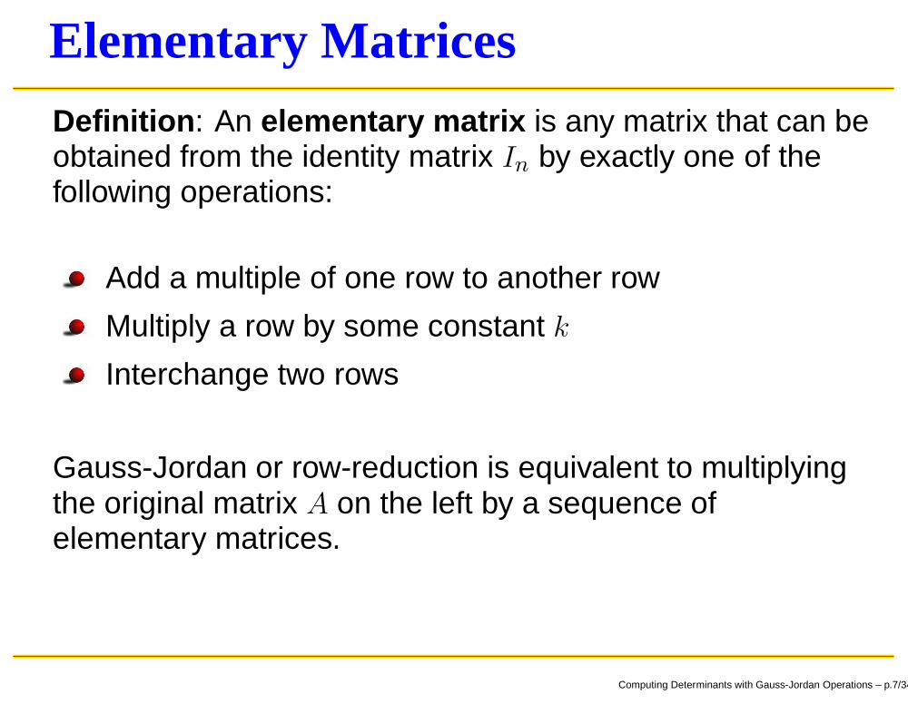
Elementary MatricesDefinition : An elementary matrix is any matrix that can beobtained from the identity matrix In by exactly one of thefollowing operations:
Add a multiple of one row to another row
Multiply a row by some constant k
Interchange two rows
Gauss-Jordan or row-reduction is equivalent to multiplyingthe original matrix A on the left by a sequence ofelementary matrices.
Computing Determinants with Gauss-Jordan Operations – p.7/34
Elementary MatricesDefinition : An elementary matrix is any matrix that can beobtained from the identity matrix In by exactly one of thefollowing operations:
Add a multiple of one row to another row
Multiply a row by some constant k
Interchange two rows
Gauss-Jordan or row-reduction is equivalent to multiplyingthe original matrix A on the left by a sequence ofelementary matrices.
We will examine this assertion in more detail.
Computing Determinants with Gauss-Jordan Operations – p.7/34

Elementary MatricesAdd a multiple of one row to another row
Start with an identity matrix
1
1. . .
1
Computing Determinants with Gauss-Jordan Operations – p.8/34
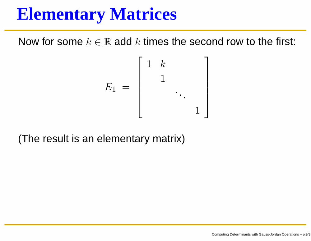
Elementary MatricesNow for some k ∈ R add k times the second row to the first:
E1 =
1 k
1. . .
1
(The result is an elementary matrix)
Computing Determinants with Gauss-Jordan Operations – p.9/34

Elementary MatricesConsider the effect of multiplying an arbitrary n × n matrix A(written as a column of row vectors) on the left by thismatrix:
E1A =
1 k
1. . .
1
a1
a2
...an
=
a1 + ka2
a2
...an
Computing Determinants with Gauss-Jordan Operations – p.10/34

Elementary MatricesConsider the effect of multiplying an arbitrary n × n matrix A(written as a column of row vectors) on the left by thismatrix:
E1A =
1 k
1. . .
1
a1
a2
...an
=
a1 + ka2
a2
...an
We obtained the elementary matrix E1 by adding k timesthe second row of In to the first row.Multiplying A on the left by E1 has the same effect on A.
Computing Determinants with Gauss-Jordan Operations – p.10/34

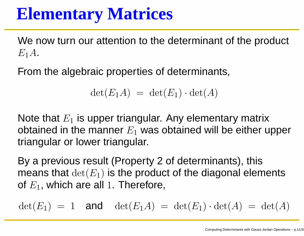
Elementary MatricesWe now turn our attention to the determinant of the productE1A.
From the algebraic properties of determinants,
det(E1A) = det(E1) · det(A)
Computing Determinants with Gauss-Jordan Operations – p.11/34

Elementary MatricesWe now turn our attention to the determinant of the productE1A.
From the algebraic properties of determinants,
det(E1A) = det(E1) · det(A)
Note that E1 is upper triangular. Any elementary matrixobtained in the manner E1 was obtained will be either uppertriangular or lower triangular.
Computing Determinants with Gauss-Jordan Operations – p.11/34
Elementary MatricesWe now turn our attention to the determinant of the productE1A.
From the algebraic properties of determinants,
det(E1A) = det(E1) · det(A)
Note that E1 is upper triangular. Any elementary matrixobtained in the manner E1 was obtained will be either uppertriangular or lower triangular.
By a previous result (Property 2 of determinants), thismeans that det(E1) is the product of the diagonal elementsof E1, which are all 1. Therefore,
det(E1) = 1 and det(E1A) = det(E1) · det(A) = det(A)
Computing Determinants with Gauss-Jordan Operations – p.11/34
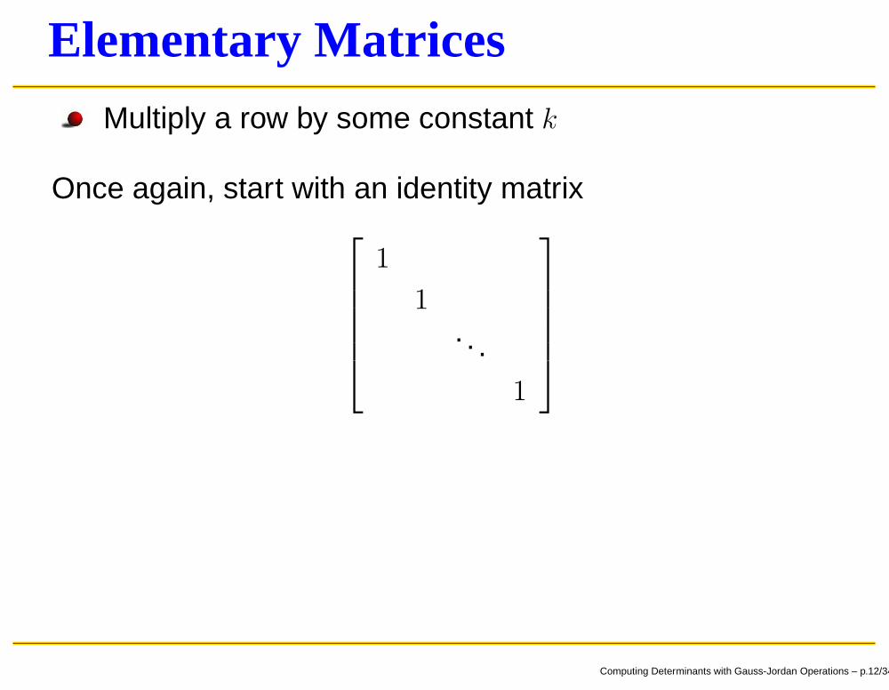
Elementary MatricesMultiply a row by some constant k
Once again, start with an identity matrix
1
1. . .
1
Computing Determinants with Gauss-Jordan Operations – p.12/34
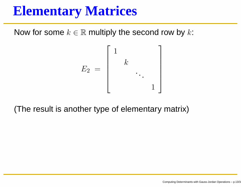
Elementary MatricesNow for some k ∈ R multiply the second row by k:
E2 =
1
k. . .
1
(The result is another type of elementary matrix)
Computing Determinants with Gauss-Jordan Operations – p.13/34

Elementary MatricesConsider the effect of multiplying an arbitrary n × n matrix A(written as a column of row vectors) on the left by thismatrix:
E2A =
1
k. . .
1
a1
a2
...an
=
a1
ka2
...an
Computing Determinants with Gauss-Jordan Operations – p.14/34
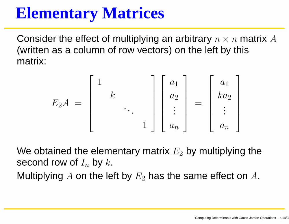
Elementary MatricesConsider the effect of multiplying an arbitrary n × n matrix A(written as a column of row vectors) on the left by thismatrix:
E2A =
1
k. . .
1
a1
a2
...an
=
a1
ka2
...an
We obtained the elementary matrix E2 by multiplying thesecond row of In by k.Multiplying A on the left by E2 has the same effect on A.
Computing Determinants with Gauss-Jordan Operations – p.14/34

Elementary MatricesNow consider the determinant of the product E2A.
From the algebraic properties of determinants,
det(E2A) = det(E2) · det(A)
Computing Determinants with Gauss-Jordan Operations – p.15/34
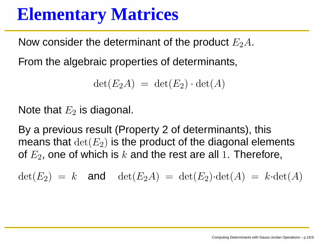
Elementary MatricesNow consider the determinant of the product E2A.
From the algebraic properties of determinants,
det(E2A) = det(E2) · det(A)
Note that E2 is diagonal.
By a previous result (Property 2 of determinants), thismeans that det(E2) is the product of the diagonal elementsof E2, one of which is k and the rest are all 1. Therefore,
det(E2) = k and det(E2A) = det(E2)·det(A) = k·det(A)
Computing Determinants with Gauss-Jordan Operations – p.15/34
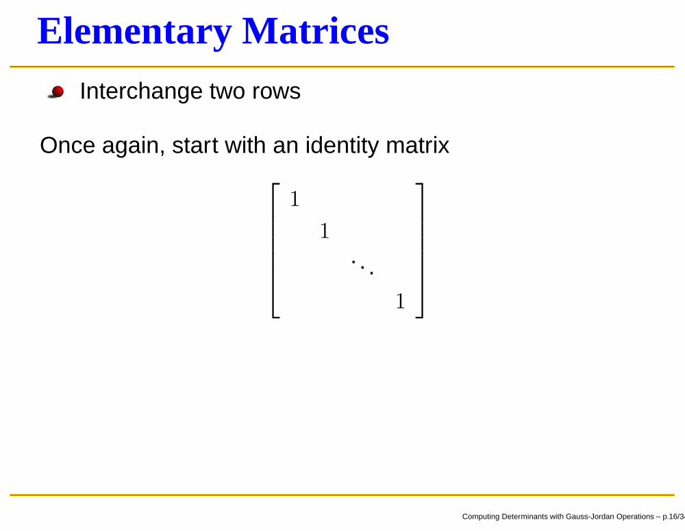
Elementary MatricesInterchange two rows
Once again, start with an identity matrix
1
1. . .
1
Computing Determinants with Gauss-Jordan Operations – p.16/34
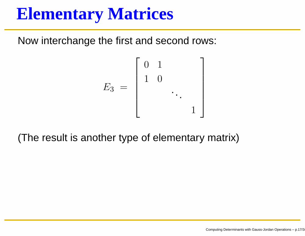
Elementary MatricesNow interchange the first and second rows:
E3 =
0 1
1 0. . .
1
(The result is another type of elementary matrix)
Computing Determinants with Gauss-Jordan Operations – p.17/34
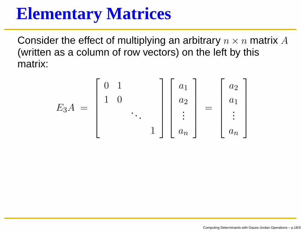
Elementary MatricesConsider the effect of multiplying an arbitrary n × n matrix A(written as a column of row vectors) on the left by thismatrix:
E3A =
0 1
1 0. . .
1
a1
a2
...an
=
a2
a1
...an
Computing Determinants with Gauss-Jordan Operations – p.18/34

Elementary MatricesConsider the effect of multiplying an arbitrary n × n matrix A(written as a column of row vectors) on the left by thismatrix:
E3A =
0 1
1 0. . .
1
a1
a2
...an
=
a2
a1
...an
We obtained the elementary matrix E3 by interchanging thefirst two rows of In.Multiplying A on the left by E3 has the same effect on A.
Computing Determinants with Gauss-Jordan Operations – p.18/34

Elementary MatricesNow consider the determinant of the product E3A.
From the algebraic properties of determinants,
det(E3A) = det(E3) · det(A)
Computing Determinants with Gauss-Jordan Operations – p.19/34
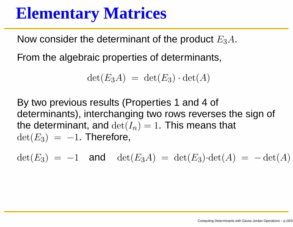
Elementary MatricesNow consider the determinant of the product E3A.
From the algebraic properties of determinants,
det(E3A) = det(E3) · det(A)
By two previous results (Properties 1 and 4 ofdeterminants), interchanging two rows reverses the sign ofthe determinant, and det(In) = 1. This means thatdet(E3) = −1. Therefore,
det(E3) = −1 and det(E3A) = det(E3)·det(A) = − det(A)
Computing Determinants with Gauss-Jordan Operations – p.19/34

Computing the DeterminantNow we can write down our algorithm for usingGauss-Jordan reduction to compute a determinant.
Starting with an arbitrary n × n matrix A, we perform aseries of row operations, each of which is equivalent tomultiplication of A on the left by some elementary matrix Ei.
After the first row operation, we have a new matrix B1,which is the product E1A:
E1A = B1
Computing Determinants with Gauss-Jordan Operations – p.20/34
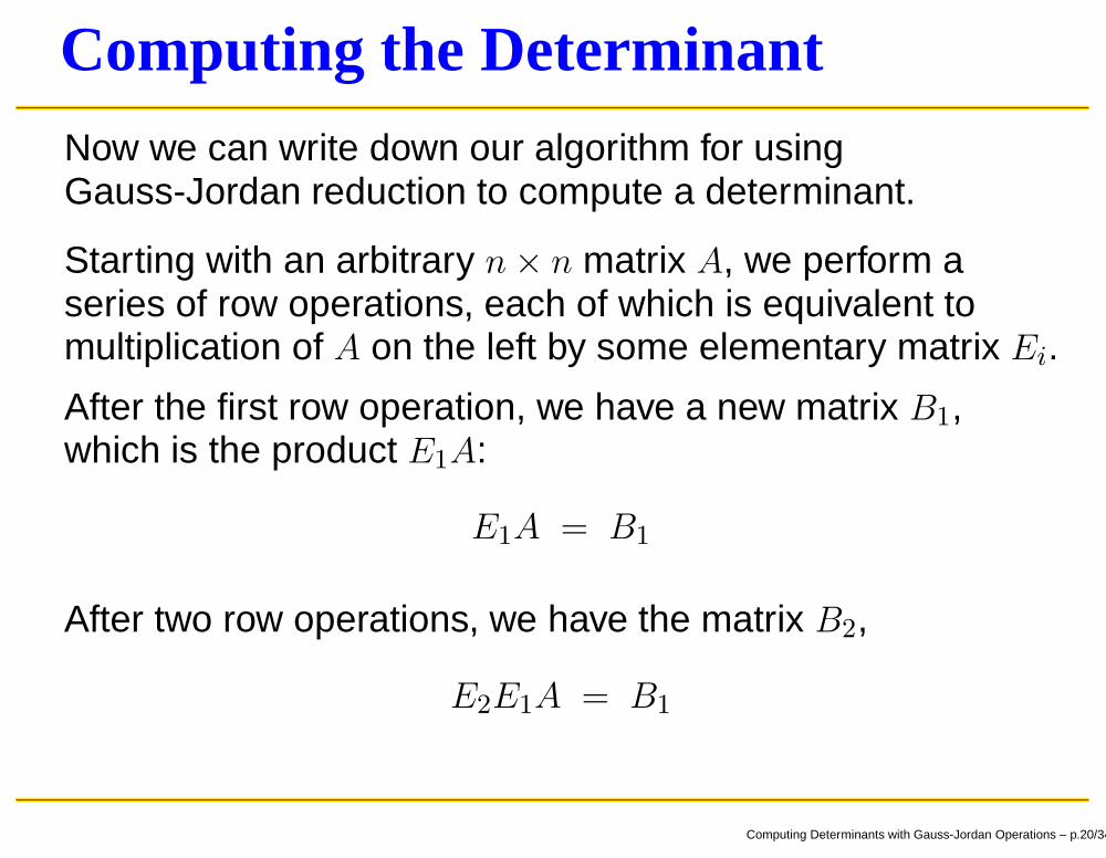
Computing the DeterminantNow we can write down our algorithm for usingGauss-Jordan reduction to compute a determinant.
Starting with an arbitrary n × n matrix A, we perform aseries of row operations, each of which is equivalent tomultiplication of A on the left by some elementary matrix Ei.
After the first row operation, we have a new matrix B1,which is the product E1A:
E1A = B1
After two row operations, we have the matrix B2,
E2E1A = B1
Computing Determinants with Gauss-Jordan Operations – p.20/34

Computing the DeterminantSuppose after k row operations, the matrix Bk is uppertriangular:
Ek · · ·E2E1A = Bk
Computing Determinants with Gauss-Jordan Operations – p.21/34

Computing the DeterminantSuppose after k row operations, the matrix Bk is uppertriangular:
Ek · · ·E2E1A = Bk
Since the determinant of a matrix product is the product ofthe determinants,
det(Ek) · · · det(E2) det(E1) det(A) = det(Bk)
Computing Determinants with Gauss-Jordan Operations – p.21/34

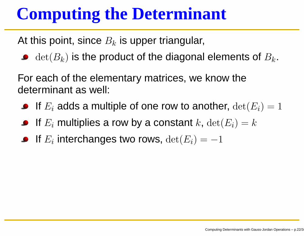
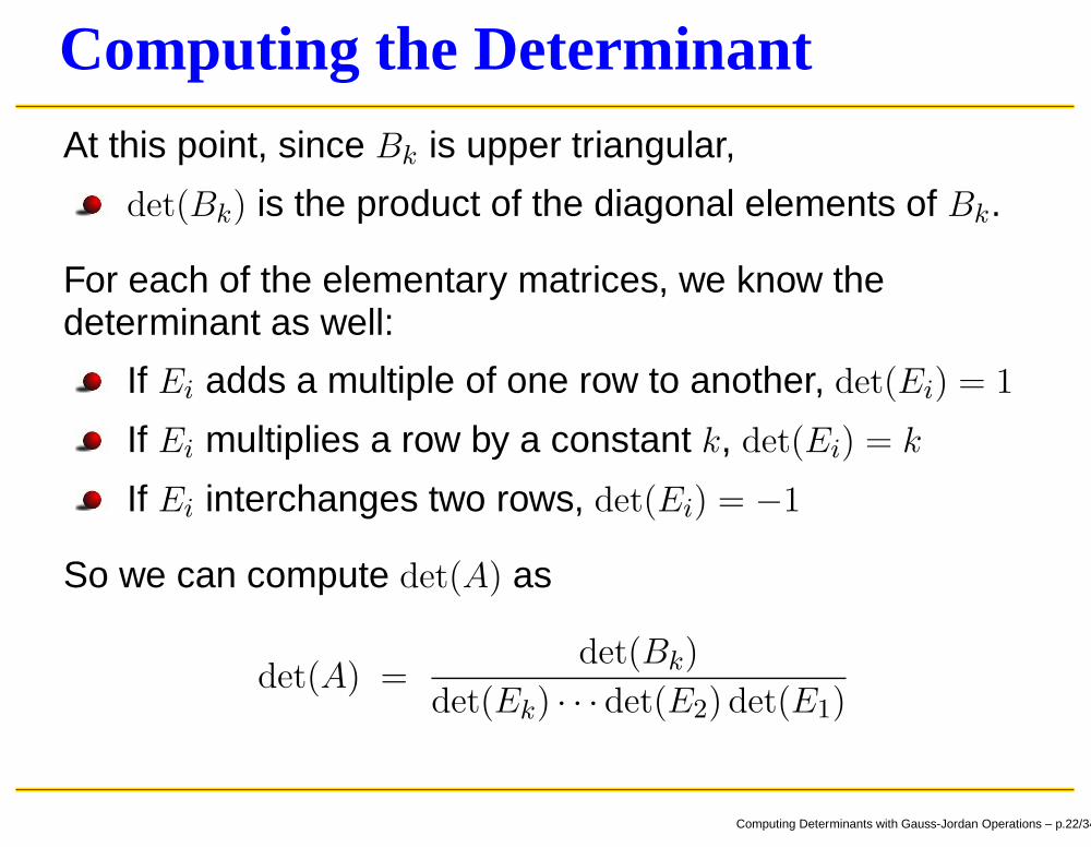
Computing the DeterminantAt this point, since Bk is upper triangular,
det(Bk) is the product of the diagonal elements of Bk.
Computing Determinants with Gauss-Jordan Operations – p.22/34
Computing the DeterminantAt this point, since Bk is upper triangular,
det(Bk) is the product of the diagonal elements of Bk.
For each of the elementary matrices, we know thedeterminant as well:
If Ei adds a multiple of one row to another, det(Ei) = 1
If Ei multiplies a row by a constant k, det(Ei) = k
If Ei interchanges two rows, det(Ei) = −1
So we can compute det(A) as
det(A) =det(Bk)
det(Ek) · · · det(E2) det(E1)
Computing Determinants with Gauss-Jordan Operations – p.22/34

Computing the DeterminantExample : Compute the determinant of
A =
2 4 −2
1 3 1
3 3 −11
Computing Determinants with Gauss-Jordan Operations – p.23/34
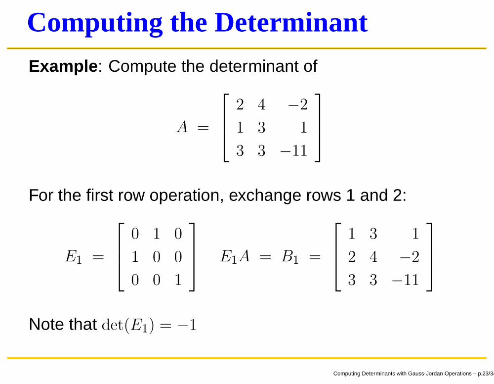
Computing the DeterminantExample : Compute the determinant of
A =
2 4 −2
1 3 1
3 3 −11
For the first row operation, exchange rows 1 and 2:
E1 =
0 1 0
1 0 0
0 0 1
E1A = B1 =
1 3 1
2 4 −2
3 3 −11
Note that det(E1) = −1
Computing Determinants with Gauss-Jordan Operations – p.23/34

Computing the DeterminantFor the second row operation, add −2 times the first row tothe second:
E2 =
1 0 0
−2 1 0
0 0 1
E2E1A = B2 =
1 3 1
0 −2 −4
3 3 −11
Note that det(E2) = 1
Computing Determinants with Gauss-Jordan Operations – p.24/34

Computing the DeterminantFor the third row operation, add −3 times the first row to thethird:
E3 =
1 0 0
0 1 0
−3 0 1
E3E2E1A = B3 =
1 3 1
0 −2 −4
0 −6 −14
Note that det(E3) = 1
Computing Determinants with Gauss-Jordan Operations – p.25/34

Computing the DeterminantFor the fourth row operation, multiply the second row by−1/2 to get a leading 1:
E4 =
1 0 0
0 −1
20
0 0 1
E4E3E2E1A = B4 =
1 3 1
0 1 2
0 −6 −14
Note that det(E4) = −1/2
Computing Determinants with Gauss-Jordan Operations – p.26/34
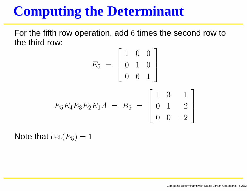
Computing the DeterminantFor the fifth row operation, add 6 times the second row tothe third row:
E5 =
1 0 0
0 1 0
0 6 1
E5E4E3E2E1A = B5 =
1 3 1
0 1 2
0 0 −2
Note that det(E5) = 1
Computing Determinants with Gauss-Jordan Operations – p.27/34

Computing the DeterminantNow since B5 is upper triangular, no more row operationsare required.
E5E4E3E2E1A = B5 =
1 3 1
0 1 2
0 0 −2
Computing Determinants with Gauss-Jordan Operations – p.28/34

Computing the DeterminantNow since B5 is upper triangular, no more row operationsare required.
E5E4E3E2E1A = B5 =
1 3 1
0 1 2
0 0 −2
Note that det(B5) = 1 · 1 · −2 = −2
Now we can write
det(E5) det(E4) det(E3) det(E2) det(E1) det(A) = det(B5)
Computing Determinants with Gauss-Jordan Operations – p.28/34

Computing the DeterminantSo
det(A) =det(B5)
det(E5) det(E4) det(E3) det(E2) det(E1)
Computing Determinants with Gauss-Jordan Operations – p.29/34
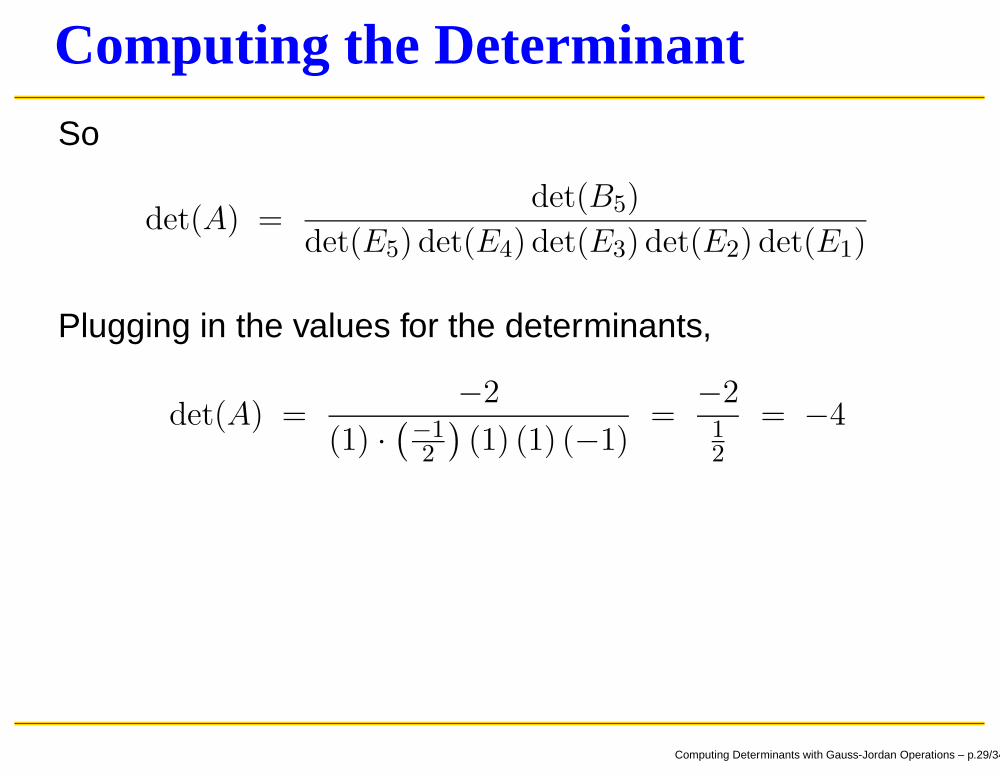
Computing the DeterminantSo
det(A) =det(B5)
det(E5) det(E4) det(E3) det(E2) det(E1)
Plugging in the values for the determinants,
det(A) =−2
(1) ·(
−1
2
)
(1) (1) (−1)=
−21
2
= −4
Computing Determinants with Gauss-Jordan Operations – p.29/34

Computing the DeterminantExample : Compute the determinant of
A =
1 2 3
4 9 12
5 11 15
Computing Determinants with Gauss-Jordan Operations – p.30/34

Computing the DeterminantExample : Compute the determinant of
A =
1 2 3
4 9 12
5 11 15
For the first row operation, add −4 times the first row to thesecond:
E1 =
1 0 0
−4 1 0
0 0 1
E1A = B1 =
1 2 3
0 1 0
5 11 15
Note that det(E1) = 1
Computing Determinants with Gauss-Jordan Operations – p.30/34

Computing the DeterminantFor the second row operation, add −5 times the first row tothe third:
E2 =
1 0 0
0 1 0
−5 0 1
E2E1A = B2 =
1 2 3
0 1 0
0 1 0
Note that det(E2) = 1
Computing Determinants with Gauss-Jordan Operations – p.31/34
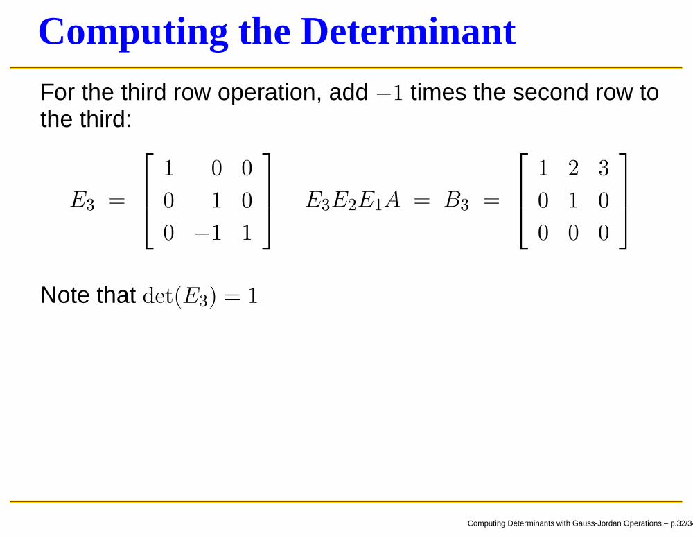
Computing the DeterminantFor the third row operation, add −1 times the second row tothe third:
E3 =
1 0 0
0 1 0
0 −1 1
E3E2E1A = B3 =
1 2 3
0 1 0
0 0 0
Note that det(E3) = 1
Computing Determinants with Gauss-Jordan Operations – p.32/34

Computing the DeterminantNo more row operations are required because B3 is uppertriangular, and so the determinant is the product of thediagonal entries:
det(B3) = 1 · 1 · 0 = 0
Computing Determinants with Gauss-Jordan Operations – p.33/34

Computing the DeterminantNo more row operations are required because B3 is uppertriangular, and so the determinant is the product of thediagonal entries:
det(B3) = 1 · 1 · 0 = 0
SinceE3E2E1A = B3
det(E3) det(E2) det(E1) det(A) = det(B3)
Computing Determinants with Gauss-Jordan Operations – p.33/34
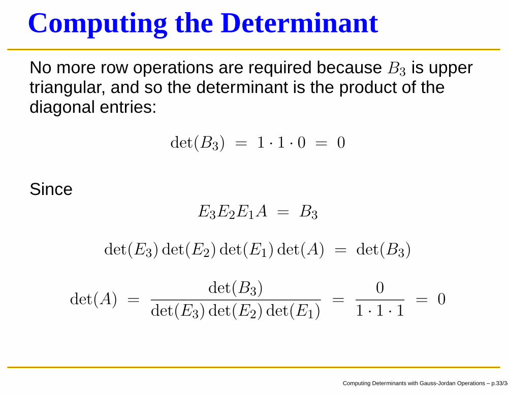
Computing the DeterminantNo more row operations are required because B3 is uppertriangular, and so the determinant is the product of thediagonal entries:
det(B3) = 1 · 1 · 0 = 0
SinceE3E2E1A = B3
det(E3) det(E2) det(E1) det(A) = det(B3)
det(A) =det(B3)
det(E3) det(E2) det(E1)=
0
1 · 1 · 1= 0
Computing Determinants with Gauss-Jordan Operations – p.33/34

Computing the DeterminantNote that
B3 =
1 2 3
0 1 0
0 0 0
so
rref(A) =
1 0 3
0 1 0
0 0 0
6= I3
which indicates that A does not have an inverse.
Computing Determinants with Gauss-Jordan Operations – p.34/34

Computing the DeterminantNote that
B3 =
1 2 3
0 1 0
0 0 0
so
rref(A) =
1 0 3
0 1 0
0 0 0
6= I3
which indicates that A does not have an inverse.
This is consistent with the fact that det(A) = 0.
Computing Determinants with Gauss-Jordan Operations – p.34/34