School of Computing, Engineering & Physical Sciences

Computing and Information Systems JournalVol 23, No 2, 2019Edited by Abel Usoro

www.uws.ac.uk

© University of the West of Scotland, 2018

All authors of articles published in this journal are entitled to copy or republish their own work in other journals or conferences. Permission is hereby granted to others for the publication of attributed extracts, quotations and citations of material from this journal. No other mode of publication or copying of any part of this publication is permitted without the explicit permission of the University.

Computing and Information Systems is published normally three times per year, in February, May, and October, by the University of the West of Scotland.

The editorial address is Dr Abel Usoro, School of Computing, Engineering & Physical Sciences,University of the West of Scotland, High Street, Paisley PA1 2BE, UK.Tel (+44) 141 848 3959; fax (+44) 141 848 3542, e-mail: cis@uws.ac.uk or abel.usoro@uws.ac.uk

Editorial Policy

Computing and Information Systems offers an opportunity for the development of novel approaches, and the reinterpretation and further development of traditional methodologies taking into account the rate of change in computing technology, and its usage and impact in organisations. Computing and Information Systems welcomes articles and short communications in a range of disciplines:

• Organisational Information Systems• Computational Intelligence• E-Business• Knowledge and Information Management• Interactive and Strategic Systems• Engineering• E-Learning• Cloud Computing• Computing Science

The website for Computing and Information Systems is http://cis.uws.ac.uk

Methodology for Image Cryptosystem Based on a Gray Code Number System

Babatunde Akinbowale Nathaniel

Department of Computer Science, Kwara State University, Malete, Nigeria. akinbowale.babatunde@kwasu.edu.ng

ABSTRACT Purpose: This paper presents a methodology for an image cryptosystem to ameliorate the problems of many existing digital image cryptosystems. The cryptosystem is based on a gray code number system. Design/Methodology/Approach: The gray code number system design is used to transform the pixel information of an image. Images are first binarized and based on the location of a particular pixel value an algorithm is selected for its transformation. This is later followed by a gray code transformation and reconstruction of the image (cipher). Findings: Based on the mathematical analysis performed with the encryption and decryption designs, it is being envisaged that the proposed technique will efficiently encrypt digital images. Research Limitation: This paper only presents the methodology for image cryptosystem based on the gray code number system. The designed system is yet to be implemented and tested to confirm its efficiency. Originality/Value: In the literature, a lot has been done in the area of applying unconventional number system in image encoding but this research laid emphasis on the use of gray code number system in image security. Many recent journals were considered. Keywords: Gray code, spatial domain, image scrambling, image encryption, Java programming. Paper Type: Research Paper. 1 Introduction A digital image can be defined as an m by n rectangular array of dots, where m is the number of rows and n is the number of columns. In technical terms, m by n is the resolution of the digital image and the dots are called the picture elements. A pixel is a small square with two

properties; pixel location and color. Hence, a frame with width W pixels and a height H pixels has a frame size of W*H pixels (Babatunde, Jimoh & Gbolagade, 2016). Basically, the fineness of an image represents the number of pixels per unit area (dpi) (Rhoma & Abobaker, 2010).

Pixel numerical values typically represent gray levels, colors, heights, opacities etc. The RGB color system is a usual technique for representing colors in digital images and thus a digital image consists of a width, a height, and a set of color quantity accessible by means of (x, y) coordinates. A color value is made up of a tuple (r, g, b), where the variables refer to the integer values of its red, green, and blue components, respectively (Wikipedia, 2017).

Every digital device/ system design depends so much on the number systems (Abdul-Barik, 2016). There are two (2) types of number systems: the conventional or positional (Weighted Number System) and the unconventional or the non-positional (Unweighted Number System) number systems. Digital devices/systems are mostly built around the WNS (Abdul-Barik, 2016).

The main challenge of WNS is with the carrying propagation chains in its operations and to improve the performance of processors built around WNS in terms of speed and area cost there is need to eliminate the associated inherent carry propagation.

This paper presents a digital image encoding system that is based on one of the unconventional number systems. The remaining part of the paper presents the background to the study, proposed algorithm, conclusion and future work. 2 Background An image P is a rectangular array of intensity values!𝑝#,%&#,%'(

),*. For grey-level images, the value

Pi, j is a single number, while for color images Pi, j

1

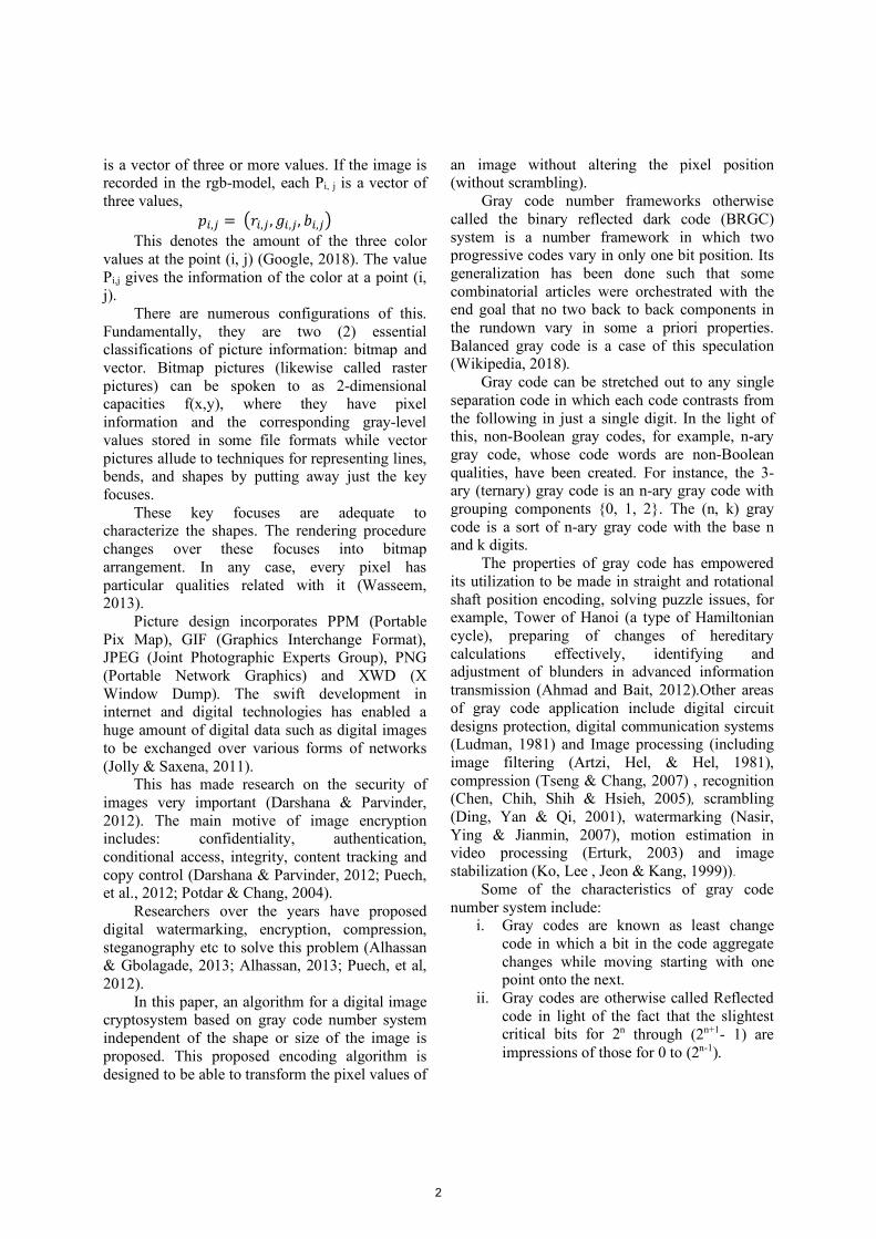
is a vector of three or more values. If the image is recorded in the rgb-model, each Pi, j is a vector of three values,

𝑝#,% = -𝑟#,% , 𝑔#,%, 𝑏#,%1 This denotes the amount of the three color

values at the point (i, j) (Google, 2018). The value Pi,j gives the information of the color at a point (i, j).

There are numerous configurations of this. Fundamentally, they are two (2) essential classifications of picture information: bitmap and vector. Bitmap pictures (likewise called raster pictures) can be spoken to as 2-dimensional capacities f(x,y), where they have pixel information and the corresponding gray-level values stored in some file formats while vector pictures allude to techniques for representing lines, bends, and shapes by putting away just the key focuses.

These key focuses are adequate to characterize the shapes. The rendering procedure changes over these focuses into bitmap arrangement. In any case, every pixel has particular qualities related with it (Wasseem, 2013).

Picture design incorporates PPM (Portable Pix Map), GIF (Graphics Interchange Format), JPEG (Joint Photographic Experts Group), PNG (Portable Network Graphics) and XWD (X Window Dump). The swift development in internet and digital technologies has enabled a huge amount of digital data such as digital images to be exchanged over various forms of networks (Jolly & Saxena, 2011).

This has made research on the security of images very important (Darshana & Parvinder, 2012). The main motive of image encryption includes: confidentiality, authentication, conditional access, integrity, content tracking and copy control (Darshana & Parvinder, 2012; Puech, et al., 2012; Potdar & Chang, 2004).

Researchers over the years have proposed digital watermarking, encryption, compression, steganography etc to solve this problem (Alhassan & Gbolagade, 2013; Alhassan, 2013; Puech, et al, 2012).

In this paper, an algorithm for a digital image cryptosystem based on gray code number system independent of the shape or size of the image is proposed. This proposed encoding algorithm is designed to be able to transform the pixel values of

an image without altering the pixel position (without scrambling).

Gray code number frameworks otherwise called the binary reflected dark code (BRGC) system is a number framework in which two progressive codes vary in only one bit position. Its generalization has been done such that some combinatorial articles were orchestrated with the end goal that no two back to back components in the rundown vary in some a priori properties. Balanced gray code is a case of this speculation (Wikipedia, 2018).

Gray code can be stretched out to any single separation code in which each code contrasts from the following in just a single digit. In the light of this, non-Boolean gray codes, for example, n-ary gray code, whose code words are non-Boolean qualities, have been created. For instance, the 3-ary (ternary) gray code is an n-ary gray code with grouping components {0, 1, 2}. The (n, k) gray code is a sort of n-ary gray code with the base n and k digits.

The properties of gray code has empowered its utilization to be made in straight and rotational shaft position encoding, solving puzzle issues, for example, Tower of Hanoi (a type of Hamiltonian cycle), preparing of changes of hereditary calculations effectively, identifying and adjustment of blunders in advanced information transmission (Ahmad and Bait, 2012).Other areas of gray code application include digital circuit designs protection, digital communication systems (Ludman, 1981) and Image processing (including image filtering (Artzi, Hel, & Hel, 1981), compression (Tseng & Chang, 2007) , recognition (Chen, Chih, Shih & Hsieh, 2005), scrambling (Ding, Yan & Qi, 2001), watermarking (Nasir, Ying & Jianmin, 2007), motion estimation in video processing (Erturk, 2003) and image stabilization (Ko, Lee , Jeon & Kang, 1999)).

Some of the characteristics of gray code number system include:

i. Gray codes are known as least change code in which a bit in the code aggregate changes while moving starting with one point onto the next.

ii. Gray codes are otherwise called Reflected code in light of the fact that the slightest critical bits for 2n through (2n+1- 1) are impressions of those for 0 to (2n-1).

2

iii. Gray codes are otherwise called unweighted code which implies the bit positions in the code do not have a particular weight doled out (non-positional).

iv. Gray codes are otherwise called cyclic (continually being created by a component) codes or unit separate codes in which the contrast between the code bunches varies just by 1.

The Gray code characteristic as minimum change code ensures that if we go from one decimal number to the next, only one bit of the gray code changes. As a result of this, the amount of switching is minimized and its reliability by switching systems is improved. Also, errors are easily detected. These features make the gray code number system advantageous.

Gray code is an un-weighted number system. There are no specific weights assigned to the bit positions and because of this the number system is unsuitable for arithmetic operations.

In an offer to display gray code number system with more broad attributes and make it suitable for applications in imaging system, another sort of n-ary gray code called the (n, k, p) gray code was proposed in 2013. The proposed design presented a distance parameter p with the idea of the (n, k) gray code (Zhou, Karen, Sas and Chen, 2013).

From its name, this kind of gray code number system utilizes non-flag values in its encoding with the end goal that numbers are spoken to in any base n (Stojmenovic, 1996). The (n, k) gray code is the n-ary gray code with k digits (Guan, 1998). Different sorts of gray code number systems incorporate gray-code, Monotonic gray codes, Beckett gray code named after Samuel Becket, Snake-in-the-crate codes, Single-track Gray code which is helpful in locating error (Google, 2018).

Zhou et al. (2013) proposed another kind of n-ary gray code called the (n, k, p) gray code. As prior clarified, it presents a new distant parameter p with the idea of the (n, k) gray code. The new (n, k, p) gray code changes as the estimations of the base n and the distant parameter p differ. Let us consider two non-negative whole numbers I and G of k-bits with base n, which is defined as (ak-1, ..., a3, a2, a1, a0)n and (gk-1, ... , g3, g2, g1, g0)n respectively that is A= ∑ 𝑎#45(

#'6 𝑛# and G=

∑ 𝑔#45(#'6 𝑛#. The (n, k, p) gray code of A is called G

and if the sequences are satisfied with the following equations: 𝑔#= 8

𝑎# ,𝑖𝑓𝑖 > 𝑘 − 𝑝 − 2(𝑎# +𝑎# + 𝑝 + 1)𝑚𝑜𝑑𝑛,𝑖𝑓0 ≤ 𝑖 ≤ 𝑘 − 𝑝 − 2

The (n, k, p) gray code can be defined by the following matrix form. If p = 0 and k = 8, then the matrix can be shown as:

⎝

⎜⎜⎜⎜⎛

𝑔K𝑔L𝑔M𝑔N𝑔O𝑔P𝑔(𝑔6⎠

⎟⎟⎟⎟⎞

=

⎝

⎜⎜⎜⎜⎜⎛

⎝

⎜⎜⎜⎜⎛

11000000

01100000

00110000

00011000

00001100

00000110

00000011

00000001⎠

⎟⎟⎟⎟⎞

×

⎝

⎜⎜⎜⎜⎛

𝑎K𝑎L𝑎M𝑎N𝑎O𝑎P𝑎(𝑎6⎠

⎟⎟⎟⎟⎞

⎠

⎟⎟⎟⎟⎟⎞

𝑚𝑜𝑑𝑛

If p = 1, k = 8 and n = 2, then the matrix can be shown as:

⎝

⎜⎜⎜⎜⎛

𝑔K𝑔L𝑔M𝑔N𝑔O𝑔P𝑔(𝑔6⎠

⎟⎟⎟⎟⎞

=

⎝

⎜⎜⎜⎜⎜⎛

⎝

⎜⎜⎜⎜⎛

10100000

01010000

00101000

00010100

00001010

00000101

00000010

00000001⎠

⎟⎟⎟⎟⎞

×

⎝

⎜⎜⎜⎜⎛

𝑎K𝑎L𝑎M𝑎N𝑎O𝑎P𝑎(𝑎6⎠

⎟⎟⎟⎟⎞

⎠

⎟⎟⎟⎟⎟⎞

𝑚𝑜𝑑2

By choosing values of the base n and distant

parameter p, the (n, k, p) gray code produces distinctive gray codes, including several conventional gray codes, for example, the one displayed underneath:

i. For p = 0, the (n, k, p) gray code swings back to the (n, k) gray code.

ii. For n = 2 and p = 0, the (n, k, p) gray code changes to BRGC.

iii. For n = 3 and p = 0, the (n, k, p) gray code returns to the regular ternary gray code.

iv. If n is another esteem, the (n, k, p) gray code will be other kind of gray code another kind of gray codes.

3

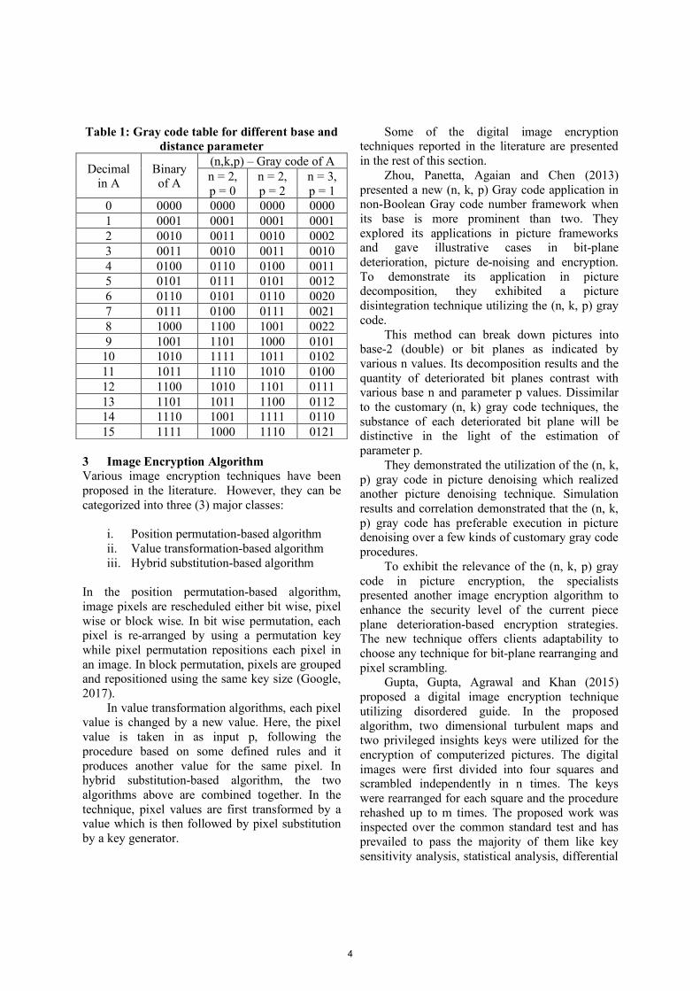
Table 1: Gray code table for different base and distance parameter

Decimal in A

Binary of A

(n,k,p) – Gray code of A n = 2, p = 0

n = 2, p = 2

n = 3, p = 1

0 0000 0000 0000 0000 1 0001 0001 0001 0001 2 0010 0011 0010 0002 3 0011 0010 0011 0010 4 0100 0110 0100 0011 5 0101 0111 0101 0012 6 0110 0101 0110 0020 7 0111 0100 0111 0021 8 1000 1100 1001 0022 9 1001 1101 1000 0101

10 1010 1111 1011 0102 11 1011 1110 1010 0100 12 1100 1010 1101 0111 13 1101 1011 1100 0112 14 1110 1001 1111 0110 15 1111 1000 1110 0121

3 Image Encryption Algorithm Various image encryption techniques have been proposed in the literature. However, they can be categorized into three (3) major classes:

i. Position permutation-based algorithm ii. Value transformation-based algorithm iii. Hybrid substitution-based algorithm

In the position permutation-based algorithm, image pixels are rescheduled either bit wise, pixel wise or block wise. In bit wise permutation, each pixel is re-arranged by using a permutation key while pixel permutation repositions each pixel in an image. In block permutation, pixels are grouped and repositioned using the same key size (Google, 2017).

In value transformation algorithms, each pixel value is changed by a new value. Here, the pixel value is taken in as input p, following the procedure based on some defined rules and it produces another value for the same pixel. In hybrid substitution-based algorithm, the two algorithms above are combined together. In the technique, pixel values are first transformed by a value which is then followed by pixel substitution by a key generator.

Some of the digital image encryption techniques reported in the literature are presented in the rest of this section.

Zhou, Panetta, Agaian and Chen (2013) presented a new (n, k, p) Gray code application in non-Boolean Gray code number framework when its base is more prominent than two. They explored its applications in picture frameworks and gave illustrative cases in bit-plane deterioration, picture de-noising and encryption. To demonstrate its application in picture decomposition, they exhibited a picture disintegration technique utilizing the (n, k, p) gray code.

This method can break down pictures into base-2 (double) or bit planes as indicated by various n values. Its decomposition results and the quantity of deteriorated bit planes contrast with various base n and parameter p values. Dissimilar to the customary (n, k) gray code techniques, the substance of each deteriorated bit plane will be distinctive in the light of the estimation of parameter p.

They demonstrated the utilization of the (n, k, p) gray code in picture denoising which realized another picture denoising technique. Simulation results and correlation demonstrated that the (n, k, p) gray code has preferable execution in picture denoising over a few kinds of customary gray code procedures.

To exhibit the relevance of the (n, k, p) gray code in picture encryption, the specialists presented another image encryption algorithm to enhance the security level of the current piece plane deterioration-based encryption strategies. The new technique offers clients adaptability to choose any technique for bit-plane rearranging and pixel scrambling.

Gupta, Gupta, Agrawal and Khan (2015) proposed a digital image encryption technique utilizing disordered guide. In the proposed algorithm, two dimensional turbulent maps and two privileged insights keys were utilized for the encryption of computerized pictures. The digital images were first divided into four squares and scrambled independently in n times. The keys were rearranged for each square and the procedure rehashed up to m times. The proposed work was inspected over the common standard test and has prevailed to pass the majority of them like key sensitivity analysis, statistical analysis, differential

4

examination, entropy analysis, which make the proposed algorithm adequate for real time secure correspondence.

Pareek (2015) utilized the tenets of the session of chess in the plan of an image encryption plot. In his method, he utilized the knight moving guidelines and an outer mystery key of 128-bits size to plan an advanced picture encryption framework for grey images. The pictures were first separated into a few squared sub-pictures and knight visit was then used to scramble the pixels of the sub-pictures.

The beginning position of knight on a board (sub-picture) and an additional pixel substitution relies upon the algorithm used. The proposed encryption plot has an aggregate of fifteen (15) rounds and each round has four distinct procedures. The execution of the encryption scheme demonstrates that the proposed plot has a decent statistical character, key sensitivity and can oppose any attack effectively. Be that as it may, the plan can just encode N by N computerized pictures. Sivakumar and Venkatesan (2016) proposed an image encryption strategy utilizing Knight's movement way and genuine irregular number stream created using noise audio file. It was tested and the acquired outcomes were given the Lena, Baboon and Cameraman pictures of size 256 by 256 pixels and two audio files.

The adequacy of the proposed strategy is validated by statistical analysis, visual testing, entropy analysis and execution time. Relationship between nearby pixels of the encoded image is near zero and NPCR esteem is satisfactory as it is more prominent than 99.5%. The UACI value between the first picture and cipher picture is more prominent than 27.8% and firmly coordinating with the current strategies while UACI value between images is more prominent than 33% for the proposed technique. Their technique limits the likelihood of statistical, differential and entropy attacks. The unscrambling procedure is performed to affirm the recovery of the initial picture. Their work has the restriction of having the capacity to encode just N by N computerized pictures.

Yadav, Singh and Sriwas (2017) demonstrated the applicability of the (n, k, p) gray code in image encryption. They presented a hybrid image encryption methodology to enhance the security level of existing piece plane decomposition and Affine Transform based

encryption strategies. The proposed technique begins with (n, k, p) dark code bit plane decomposition and after that it revamped each piece plane utilizing arbitrary scrambling.

This is at last taken after by pixel substitution in the light of XOR Operation. This technique offers the clients adaptability to choose any technique for bit plane rearranging and pixel scrambling. The trial results and examination introduced demonstrates that the encryption algorithm delivered great execution in image encryption. It could be utilized for securing protection in biometrics, medicinal imaging frameworks, and video reconnaissance frameworks. 4 Proposed Algorithm The aim of this paper is to come up with an algorithm for a digital image cryptosystem that can encode binary representations of m by n images such that 2 neighboring pixel values with the same RGB information will have different cipher information. The algorithm will be employing the advantages and interesting properties of gray code arithmetic. The algorithm is divided into two (2) phases:

The first phase is designed to encode the binary representation of images to gray code values. G is the (n, k, p) gray code of k bits base-n nonnegative image X if the sequences are satisfied with 𝐺 = -𝐶W ∗𝑋1𝑚𝑜𝑑𝑛 where 𝐶W is a constant for converting binary to gray-code and n is the base. If 𝐶W = 𝑀W then G will be (n, k) gray code, if 𝐶W =𝑂W then G will be (n, k, p) gray code with distant parameter (p) of 2.

𝑀W =

⎝

⎜⎜⎜⎜⎛

11000000

01100000

00110000

00011000

00001100

00000110

00000011

00000001

⎠

⎟⎟⎟⎟⎞

5

𝑂W =

⎝

⎜⎜⎜⎜⎛

10010000

01001000

00100100

00010010

00001001

00000100

00000010

00000001

⎠

⎟⎟⎟⎟⎞

If p = 0 and k = 8, then the matrix can be

shown as:

⎝

⎜⎜⎜⎜⎛

𝑔K𝑔L𝑔M𝑔N𝑔O𝑔P𝑔(𝑔6⎠

⎟⎟⎟⎟⎞

=

⎝

⎜⎜⎜⎜⎜⎛

⎝

⎜⎜⎜⎜⎛

11000000

01100000

00110000

00011000

00001100

00000110

00000011

00000001⎠

⎟⎟⎟⎟⎞

×

⎝

⎜⎜⎜⎜⎛

𝑥K𝑥L𝑥M𝑥N𝑥O𝑥P𝑥(𝑥6⎠

⎟⎟⎟⎟⎞

⎠

⎟⎟⎟⎟⎟⎞

𝑚𝑜𝑑𝑛

If p = 2, k = 8 and n = 2, then the matrix can

be shown as:

⎝

⎜⎜⎜⎜⎛

𝑔K𝑔L𝑔M𝑔N𝑔O𝑔P𝑔(𝑔6⎠

⎟⎟⎟⎟⎞

=

⎝

⎜⎜⎜⎜⎜⎛

⎝

⎜⎜⎜⎜⎛

10010000

01001000

00100100

00010010

00001001

00000100

00000010

00000001⎠

⎟⎟⎟⎟⎞

×

⎝

⎜⎜⎜⎜⎛

𝑥K𝑥L𝑥M𝑥N𝑥O𝑥P𝑥(𝑥6⎠

⎟⎟⎟⎟⎞

⎠

⎟⎟⎟⎟⎟⎞

𝑚𝑜𝑑2

The second phase is used to encrypt the pixel

values of m by n images such that two neighboring pixel values with the same RGB information will not have the same cipher information. In a bid to achieve this, each pixel location is scanned based on the result of the scan. An algorithm is selected to encrypt the pixel location. There are four possible algorithms to be selected from and this formula helps with the operation.

Algorithm to be selected = ((i * width length) + j) mod 4

If the result is 0 an algorithm style is selected, if 1 another unique algorithm is selected; 2 and 3 are the same. 4.1 Encryption Process The encryption scheme consists of four steps, i.e. image conversion in binary codes, algorithm

selection based on pixel position, gray-code transformation and reconstruction of RBG information. Step 1: Image conversion in binary code This involves selecting each pixel and transforming the RGB information into binary such that a Hexadecimal 𝐹𝐹 _` becomes11111111P. Step 2: Algorithm selection based on pixel position This involves selecting algorithm for a pixel based on its location. Algorithm to be selected = ((i * width length) + j ) mod 4 Step 3: Gray-code transformation The (n, k, p) gray code of A is called G and if the sequences are satisfied with the following equations 𝑔#= 8

𝑎#,𝑖𝑓𝑖 > 𝑘 − 𝑝 − 2(𝑎# + 𝑎# + 𝑝 + 1)𝑚𝑜𝑑𝑛,𝑖𝑓0 ≤ 𝑖 ≤ 𝑘 − 𝑝 − 2

we can define the (n, k, p) gray code by following a matrix form. If p = 0 and k = 8, then the matrix can be shown as:

⎝

⎜⎜⎜⎜⎛

𝑔K𝑔L𝑔M𝑔N𝑔O𝑔P𝑔(𝑔6⎠

⎟⎟⎟⎟⎞

=

⎝

⎜⎜⎜⎜⎜⎛

⎝

⎜⎜⎜⎜⎛

11000000

01100000

00110000

00011000

00001100

00000110

00000011

00000001⎠

⎟⎟⎟⎟⎞

×

⎝

⎜⎜⎜⎜⎛

𝑥K𝑥L𝑥M𝑥N𝑥O𝑥P𝑥(𝑥6⎠

⎟⎟⎟⎟⎞

⎠

⎟⎟⎟⎟⎟⎞

𝑚𝑜𝑑𝑛

If p = 2, k = 8 and n = 2, then the matrix can

be shown as:

⎝

⎜⎜⎜⎜⎛

𝑔K𝑔L𝑔M𝑔N𝑔O𝑔P𝑔(𝑔6⎠

⎟⎟⎟⎟⎞

=

⎝

⎜⎜⎜⎜⎜⎛

⎝

⎜⎜⎜⎜⎛

10010000

01001000

00100100

00010010

00001001

00000100

00000010

00000001⎠

⎟⎟⎟⎟⎞

×

⎝

⎜⎜⎜⎜⎛

𝑥K𝑥L𝑥M𝑥N𝑥O𝑥P𝑥(𝑥6⎠

⎟⎟⎟⎟⎞

⎠

⎟⎟⎟⎟⎟⎞

𝑚𝑜𝑑2

Step 4: Reconstruction of RBG information After all (n, k, p) transformation have been done, the generated cipher information will be translated back into Hexadecimal and then an encrypted image is created and stored.

6

4.2 Pseudocode for the encryption process The pseudocode for the encryption process is as follows:

Begin Input the image file

Define M as an array containing constant for transforming Binary to Gary Code Define O as an array containing a constant for transforming Binary to Gary code with distance parameter of 2

Determine the image size Determine the image width and height Calculate Pixel = (width * height) – 1 Extract RGB value of image file for each pixel Get the modulus of each pixel location by 4

If the modulus is 0 NewPixel.Red = M * getRed(image.pixel)

NewPixel.Green = O-1 * getGreen(image.pixel) NewPixel.Blue =Not (getBlue(image.pixel)) Else if the modulus is 1 NewPixel.Red =Not (getRed(image.pixel)) NewPixel.Green=Not (getGreen(image.pixel))

NewPixel.Blue = M * getBlue(image.pixel) Else if the modulus is 2

NewPixel.Red = M-1 * getRed(image.pixel) NewPixel.Green = Not (getGreen(image.pixel)) NewPixel.Blue = M * (getBlue(image.pixel))

Else if the modulus is 3 NewPixel.Red = O * getRed(image.pixel) NewPixel.Green = M-1 * getGreen(image.pixel) NewPixel.Blue = Not (getBlue(image.pixel))

Reconstruct the image Save the new Image as encrypted Image

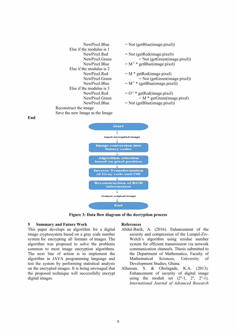
End The data flow of the encryption phase, the encryption phase flowchart and the data flow for the decryption phase is presented in figures 1, 2 and 3 respectively.

Figure 1: Data flow analysis for the Encryption phase

7

Figure 2: Flowchart for the Encryption Phase

4.3 Pseudocode of the decryption process The decryption process uses the following

pseudocode: Begin

Input the encrypted image file Define M as an array containing constant for transforming Binary to Gary Code

Define O as an array containing a constant for transforming Binary to Gary code with distance parameter of 2

Determine the image size Determine the image width and height

Calculate Pixel = (width * height) – 1 Extract RGB value of image file for each pixel Get the modulus of each pixel location by 4 If the modulus is 0

NewPixel.Red = M-1 * getRed(image.pixel) NewPixel.Green = O * getGreen(image.pixel)

8

NewPixel.Blue = Not (getBlue(image.pixel)) Else if the modulus is 1

NewPixel.Red = Not (getRed(image.pixel)) NewPixel.Green = Not (getGreen(image.pixel)) NewPixel.Blue = M-1 * getBlue(image.pixel)

Else if the modulus is 2 NewPixel.Red = M * getRed(image.pixel) NewPixel.Green = Not (getGreen(image.pixel)) NewPixel.Blue = M-1 * (getBlue(image.pixel))

Else if the modulus is 3 NewPixel.Red = O-1 * getRed(image.pixel) NewPixel.Green = M * getGreen(image.pixel) NewPixel.Blue = Not (getBlue(image.pixel)) Reconstruct the image Save the new Image as the Image

End

Figure 3: Data flow diagram of the decryption process

5 Summary and Future Work This paper develops an algorithm for a digital image cryptosystem based on a gray code number system for encrypting all formats of images. The algorithm was proposed to solve the problems common to most image encryption algorithms. The next line of action is to implement the algorithm in JAVA programming language and test the system by performing statistical analysis on the encrypted images. It is being envisaged that the proposed technique will successfully encrypt digital images.

References Abdul-Barik, A. (2016). Enhancement of the

security and compression of the Lempel-Ziv-Welch’s algorithm using residue number system for efficient transmission via network communication channels. Thesis submitted to the Department of Mathematics, Faculty of Mathematical Sciences, University of Development Studies, Ghana.

Alhassan, S. & Gbolagade, K.A. (2013). Enhancement of security of digital image using the moduli set (2n-1, 2n, 2n-1). International Journal of Advanced Research

9

in Computer Engineering and Technology (IJACET). 2(7). 2223-2229.

Alhassan, S. (2013). Enhancement of security of digital image using the moduli sets. Thesis Submitted to the Department of Mathematics, Faculty of Mathematical Sciences, University of Development Studies, Ghana.

Babatunde, A. N., Jimoh, R. G. & Gbolagade, K. A. (2016). An Algorithm for a Residue Number System Based Video Encryption System, Computer Science Series Journal 14(2), 136-147.

Ben-Artzi, G., Hel-Or, H. & Hel-Or, Y. (2007). The Gray-code filter kernels. IEEE Trans. Pattern Anal. Mach. Intell, 29(3), 382-393.

Chen, W. S., Chih, K. H., Shih, S. W., & Hsieh, C. M. (2005). Personal identification technique based on human IRIS recognition with wavelet transform. IEEE ICASSP, 2, 949-952.

Darshana, H. & Parinder, S. (2012). A comprehensive survey of video encryption algorithms. International Journal of Computer Applications. 59 (1), 14-19.

Ding, W., Yan, W. & Qi, D. (2001). Digital image scrambling. Progr. Nat. Sci., 11(6), 454-460.

Erturk, S. (2003). Locally refined Gray-coded bit-plane matching for block motion estimation. 3rd ISPA, 1, 128–133.

Gupta, K., Gupta, R., Agrawal, R. & Khan, S. (2015). An Ethical Approach of Block Based Image Encryption Using Chaotic Map. International Journal of Security and Its Applications, 9(9), 105-122.

Jolly, S. & Vikas, S. (2012). Video encryption: A Survey. International Journal of Computer Science Issues. 8(2), 525-534.

Kompendiet images. (n.d.). Digital images and image formats, Retrieved from http://www.uio.no/studier/emner/matnat/math/MAT-INF1100/h08/kompendiet/images.pdf. (Accessed on 01/05/2017).

Ludman, J. (1981). Gray code generation for MPSK signals. IEEE Transmission Communication, 29(10), 1519–1522.

Nasir, I., Ying, W. & Jianmin, J. (2007). A new robust watermarking scheme for color image in spatial domain. 3rd Internation IEEE Conference. SITIS, 942–947.

Pareek, N. K. (2015). Knight‟s Tour Application in Digital Image Encryption. International

Journal of Advanced Research in Computer Science and Software Engineering, 5(9), 208-213.

Potdar, V. & Chang, E. (2004). Disguising text cryptography using image cryptography. International Network Conference in Plymouth, UK, 6 - 9 July.

Puech, W., Erkin, Z., Barni, M., Rane, S. & Lagendijk, R. L. (2012). Emerging cryptographic challenges in image and video processing. ICIP: International Conference on Image Processing, Sep., 2012, Orlando, FL, United States. 19th IEEE International Conference on Image Processing, 2629-2632.

Rhoma, E. M. & Abobaker, A. M. (2010). Mean square error minimization using interpolative block truncation coding algorithms. 2nd International Conference on Education Technology and Computer (ICETC).

Sivakumar, T. & Venkatesan, R. (2016). A New Image Encryption Method Based on Knight’s Travel Path and True Random Number. Journal of Information Science and Engineering 32, 133-152 (2016), 133-152.

Tseng, H. W. & Chang, C. C. (2007). Anti-pseudo-gray coding for VQ encoded images over noisy channels. IEEE Commun. Lett., 11(5), 443-445.

Tutorialspoint. (n.d.). Types of Images, Retrieved from https://www.tutorialspoint.com/dip/types_of_images.htm. (Accessed on 09/12/2017).

Wasseem, N. I. (2013). Image Processing, Retrieved from http://uotechnology.edu.iq/ce/lecture%202013n/4th%20Image%20Processing%20_Lectures/DIP_Lecture2.pdf. (Accessed on 18/02/2018).

Wikipedia. (n.d.). Gray Code, https://en.m.wikipedia.org/wiki/Gray_code. (Accessed on 01/07/2017).

Yadav, S. S., Singh, Y., & Sriwas, S. K. (2017). Hybrid Image Encryption Technique to Improve the Security Level by using (n, k, p) Gray Code and XOR Operation. Indian Journal of Science and Technology, 10(20).

Zhou, Y., Panetta, K., Agaian, S. & Chen, P. C. (2013, April). (n, k, p)-Gray Code for Image Systems. IEEE Transactions On Cybernetics, 42(2), 515-529.

10

A Secured and Energy Efficient Wireless Sensor Networks (WSN) Utilizing CRT-

Based Forwarding Technique

Kamaldeen Ayodele Raji and Kazeem Alagbe Gbolagade Department of Computer Science, Kwara State University, Malete, Nigeria

kamalayour2004@gmail.com and kazeem.gbolagade@kwasu.edu.ng

ABSTRACT Purpose: The purpose of this research is to design power efficient and secured WSNs. Design/Methodology/Approach: A Chinese Remainder Theorem (CRT) was used to design a secured and energy efficient network as well as a forwarding algorithm. The algorithm breaks down the information that is received by each hub in order to diminish the number of bits transmitted by each sending hub in the system. The design implements Local Closet First (LCF) to determine the best destination in order to send the message to the next hop. Simulations were used to assess the execution of the hubs. The simulations were performed on Prowler (Probabilistic Wireless Network Simulator) running under MATLAB. Findings: Vitality and reliability are the most obliging elements on the usefulness of WSNs. The results acquired demonstrates that the proposed scheme outperforms traditional methodologies as far as vitality sparing (because nodes only need to send small packets to the sink), dependability, straightforwardness and reasonable circulation of vitality utilization among all hubs in the system and in addition decrease in delay of the sent data. Also message security is enhanced because the remainders of sensed data are sent instead of data itself. The received packet is encrypted and to decrypt the message, the receiving nodes should have the moduli set which serves as the secret key. Research limitations/implications: In this research work, application level quality of service (Qos) constraints is not met. Error detection and correction is also not considered.

Originality/Value: The proposed wireless sensor networks design is one of the few designs if not the only design that addresses the integration of energy reduction and secured WSNs using CRT packet splitting algorithm with local closet first (LCF). Keywords: Wireless Sensor Networks, Fault Tolerant, Energy Efficiency, Chinese Remainder Theorem, Packet Splitting. Paper type: Research paper.

1 Introduction WSNs comprise of interconnected Sensor hubs which are sent in a huge number and are equipped for detecting, assembling, preparing and transmitting information (Sharma and Sharma, 2016). They are normally used to monitor regions, gather information and send to the base station or sink. There are considerable numbers of potential applications for sensor systems. For instance, they can be utilized in a combat zone, where they can identify and keep an eye on the adversaries or they can bolster the positive powers. Likewise, they can be utilized in shrewd security frameworks in structures and security of basic applications. They can also be utilized for habitat monitoring applications and for study changes in phenomena, for example, temperature and sound mugginess (Kianifar, Naji and Malakooti, 2015).

Wireless sensor networks are capable of sensing and forwarding the sensed data, and performing different reactions. It comprises of sensor hubs and sink hubs which for the most part have low costs, constrained vitality supply and restricted transmission; they are in charge of distinguishing occasions or detecting ecological information (Campobello, Leonardi and Palazzo, 2009). The base stations are asset more than

11

extravagant hubs and at the same time possess rich vitality sources, higher correspondence and computation capacity, and the capacity to perform ground-breaking responses. At the point when a sensor hub recognizes information to be conveyed in its checking zone, it would transmit the occasion to neighboring hubs, which in turn would forward the occasion one bounce further.

Figure 1 demonstrates a Wireless Sensor Network containing sensor hubs and the sink. A sensor hub is a modest gadget that incorporates three parts: a processing unit used to process neighborhood information, a sensing subsystem utilized for information procurement from its condition, and a wireless communication transceiver that exchanges the detecting data to the sink. These sensor hubs perform information detecting and preparing errands and furthermore speak with each other (Kianifar, Naji and Malakooti, 2015).

Figure 1: Wireless Sensor Network

WSNs are typically furnished with restricted vitality which makes them asset obliged. Thus, in this way, the most essential perspective is the means by which to limit the vitality exhaustion of hubs remembering the ultimate objective to extend the network lifetime. Sensor hub batteries of WSNs cannot be replaced or revived once deployed. Therefore, WSNs application should be designed in an energy efficient manner (Lee, Min, Choi and Lee, 2016). Also, hubs in WSN are ordinarily mass delivered and are regularly sent in neglected and unfriendly situations which now make them more susceptible to failure than other network systems (Kshirsagar and Jirapure, 2012). However, manual assessment of flawed sensor hubs after deployment is ordinarily unfeasible. In any case, numerous WSN

applications are mission-basic, and therefore requiring continuous operation. Given the characteristics and with end goal to meet application prerequisites, an anchored, dependable and vitality productive philosophy is required in WSNs (Sachan, Imam and Beg, 2012).

In this paper, a secured and energy efficient WSNs based on Chinese Remainder Theorem (CRT) bundle part sending procedure is proposed. This strategy include breaking the detected messages into a few parcels (contingent upon number of hubs in the next hop) with the end goal that every hub in the system will forward just little sub-bundles to the sink. When the sink gets all sub-bundles effectively, it would reproduce the first message. The significant purpose behind this approach is to break the information that was sent by each sending hub in order to diminish the number of bits transmitted by each sending hub in the system, therefore power utilization is reduced. The proposed scheme outflanks traditional methodologies regarding security, vitality utilization, unwavering quality, straightforwardness, and diminishment in end-to-end delay.

1.1 Fault Tolerant in WSNs A Wireless Sensor Network is appropriate in different fields, for example, information procurement in risky condition, observing of basic frameworks and military activities. The unfriendly environment affects the monitoring infrastructure of WSNs. Since sensor hubs are relied upon to work independently in unattended and conceivably threatening situations, they are powerless against deficiencies where issues are probably going to happen often and unexpectedly (Kshirsagar and Jirapure, 2012). WSNs are failure inclined because of any of the reasons like malignant assault, energy depletion, hardware disappointment and communication.

It is generally trusted that nothing is flawless in this universe; issues are likewise unavoidable in the sensor system and it is extremely important to recognize defective and working hubs (Manisha and Nandal, 2015). With the specific end goal to keep up the system nature of administration, it is necessary for WSN to have the capacity to distinguish the deficiencies and take fitting actions to deal with them. When outlining a mistake control plot for WSNs,

12

vitality proficiency is most essential. The utilization of a particular fault tolerant system relies upon the prerequisites of the system and the requirements of the sensor network. Thus, it is important to pick an ideal fault correcting code for a sensor network where both the execution and vitality utilization are considered (Arutselvan and Maheswari, 2013).

2 Literature Review There have been a few examinations on limiting energy utilization in remote systems and particularly in Wireless Sensor Networks (WSNs). At the same time, a few vitality preservation plans have been proposed for limiting the energy utilization of the radio interface. This is because radio units consume the highest amount of power when transmitting information. Duty cycling (rest/wakeup plot) and In-Network information accumulation (Anastasi, Conti, Francesco and Passarella, 2007; Fasolo, 2007) are the most well-known preservations plans. The main approach includes putting the radio transceiver in the rest mode at whatever point communications are not required and wake when gotten a bundle from a neighboring hub. Be that as it may, energy reduction is gotten to the detriment of an expanded hub multifaceted nature and system idleness.

The second approach is aimed to merge routing and data aggregation techniques by reducing the number of transmissions. In this plan, multipath steering calculations are typically utilized. Nonetheless, numerous ways could surprisingly expend more vitality than the briefest way in light of the fact that few duplicates of a similar bundle could achieve the destination. Barati, Movaghar and Sabaei (2014) observed that redundant residue number systems (RRNSs) are appropriate for use in real time wireless sensor networks applications, because it enhances real time operations, strong error control capability, energy saving, and security. The RNS has been utilized as an instrument to lessen transmission vitality and increment unwavering quality in WSNs.

In addition, Arutselvan and Maheswari (2013) proposed an approach that depends on a parcel part calculation-based CRT described by a basic particular division between numbers. The structure has low overhead in calculation, correspondence and limit, and is immune to DoS

attack. Campobello, Serrano, Leonardi and Palazzo (2010) researched a tradeoff between vitality effectiveness and unwavering quality of the CRT sending plan when obligation cycling strategies are considered. This was accomplished with a direct increment in the general unpredictability and with low overhead.

Additionally, Roshanzadeh and Saqaeeyan (2012) observed that the restricted vitality utilization prerequisites and the low many-sided quality in the sensor equipment require vitality effective blunder control and forestall high many-sided quality codes to be sent. Redundant moduli that plays no part in deciding the dynamic range was presented. This was utilized in WSNs to diminish reestablished information sending by means of any error occurring in information parcels which were centered around low multifaceted technique of error detection. The system was implemented with low data redundancy and efficient energy consuming in wireless sensor node using residue number systems. It is therefore necessary to develop proficient and secured WSNs while still conserving the limited energy of the network as well as end-to-end delay.

3 Chinese Remainder Theorem (CRT) Chinese Remainder Theorem is a hypothesis of numeric theory, which expresses that, in case one knows the remnants of the division of an entire number n by a couple of numbers, one can choose curiously whatever is left of the division of n by the consequence of these numbers, under the condition that the divisors are pairwise coprime (Gbolagade and Contofana, 2009). The CRT is an outcome about congruence's in number hypothesis and its speculations in unique variable based math (Arutselvan and Maheswari, 2013). In its essential frame, the CRT will decide a number n that at the point when partitioned by some given numbers (divisors) leave given remnants (Omondi and Premkumar, 2007).

Assume n1, ..., nk be entire numbers more prominent than 1, which are consistently called moduli or divisors. Assume N implies the consequence of the ni. The CRT hypothesis declares that if the ni are pairwise coprime, and if a1, ..., ak are numbers with the end goal that 0 ≤ ai < ni for each i, at that point there is one and just a single whole number x, to such an extent

13

that 0 ≤ x < N and the rest of the Euclidean division of x by ni is ai for each i.

This might be rewritten as follows in term of congruences: If the ni are pairwise coprimes, and if a1, ..., ak are any whole numbers, at that point there exists a whole number x to such an extent that any two such x are compatible modulo N.

x ≡ a1 (mod n1)

x ≡ a2 (mod n2) .

. .

x ≡ ak (mod nk)

In any case, all arrangements’ x of this framework are compatible modulo of the item, N = n1, n2 … nk. In this way, x ≡ y (mod ni) for all i≤i<k if and just if x ≡ y (mod N). The customary CRT is characterized as take afters: for a moduli set {m1, m2, m3,..mk} with the dynamic range M

= 1

k

imi

, the residue number (x1, x2, x3, …,

xk) can be changed over into the decimal number X, as takes after:

X = 1

1

M

k

mii ii

Mi xM

where M = 1

k

imi

, i

iMM

m , and

1

iM

is the

multiplicative inverse of Mi with respect to mi. The primary downside of CRT rises up out of the required modulo-M activity which, given that M is a somewhat vast number, this task can be tedious and fairly costly as far as territory and vitality utilization are concerned. The CRT is valuable in invert change and also a few different activities (Omondi and Premkumar, 2007).

However, the nonattendance of convey spread between the arithmetic block results in RNS fast arithmetic. This feature is beneficial for wireless sensor networks that need to perform run-time applications. RNS also has parallel operations that reduce power consumption and delay simultaneously (Barati, Movaghar & Sabaei, 2014; Gbolagade & Cantofana, 2009). Sangeetha and Pugazendi (2013) also observed that CRT likewise can be utilized to take care of issues in processing

coding. In computing it can compete with short instead of large numbers and this will make the computing-process faster and easier. In coding it can be utilized for blunder seeking and mistake controlling. The calculation permits recreating a vast whole number from its remnants modulo, an arrangement of moduli. At the point when every one of the moduli are co-prime, CRT has a straightforward single recipe, which is notable not hearty, i.e., little mistakes from any remnants may cause a substantial recreation error.

4 Packet Forwarding Technique The capacity to furnish separated administrations to clients with broadly changing necessities is becoming progressively imperative, and Internet Service Providers might want to give these separated administrations utilizing the same shared system framework. In a computer network, packet sending procedure is the handing-off of bundles starting with one system portion then onto the next by hubs (Anton, 2015). The least complex sending model, uni-throwing, includes a message (packet) being transferred from connection to interface along a chain driving from the message's source to its destination. Another sending model is communicating which requires a message (packet) to be copied and duplicated before it moves on different connections with the objective of conveying a duplicate to each gadget on the system. Numerous ways could surprisingly expend more vitality than the single most limited way on the grounds that few duplicates of a similar parcel must be sent.

Packet Processing involves a wide collection of calculations that apply to a parcel of data or information as it goes through the diverse framework parts of corresponding arrangement (Anton, 2015). Ordinarily, there are two broad classes of packet processing that line up with the organized network subdivision; these are control plane and data plane. Calculations are associated with either and each has control information in its bundle to ascertain safe transfer of the parcel of source to destination. The data content (as frequently as conceivably called the payload) of the package are used to give some substance specific change or make a substance driven move.

Packet Splitting involves breaking the first bundles into different sub-parcels before

14

transmitting them towards the hubs (Anton, 2015). The first messages are broken into a few parcels with the end goal that every hub in the system will send just little sub bundles and reproduce them back to the original messages. The breaking technique is accomplished by using the packet splitting scheme as seen in Figure 2.

Figure 2: Packet splitting (Anton, 2015)

When all sub packets are gotten accurately by the sink hub, it will rearrange them, subsequently reproducing the initial message. This system is particularly useful for those sending hubs that are more requested than others because of their location in the system. The initial messages are breaking down into a few bundles with the aim that every hub in the system will forward just little sub parcels. The system is accomplished by applying the packet splitting algorithm. Subsequently, this gives an exhaustive systematic model that enables us to determine some precise outcomes in regards to vitality utilization and multifaceted nature (Fasolo, 2007).

5 Research Methodology Packet splitting forwarding technique is the basic method for sharing information across systems on a network. Packets are transmitted between a sender interface and a receiver interface, usually on two different nodes. With the CRT for information bundling, a hub begins at an arbitrary position and assigns prime numbers to the information parcels for security reason. For these reasons interlopers would not recognize the information packet because the original message is not sent but the prime numbers are. CRT-based part is more productive than a straightforward part (Campobello and Leonardi, 2015). The major reason for using forwarding technique is to split the messages sent by the

source node so that the maximum number of bits per packet that a node has to forward is reduced, in this way the network lifetime can be expanded (Campobello and Leonardi, 2015). CRT can be planned as follows:

Given that N primes pi>1, with i∈ {1 …N}, and considering that their item M = Πi pi, at that point for any arrangement of any given whole numbers {m1,m2, . . . ,mN} there is always a novel whole number m < M that understands the arrangement of synchronous congruences m = mi

(mod pi), and it can be gotten by m =

(1

)(mod )N

i ii

c m M . The coefficients ci are

given by ci = Qiqi, where Qi= M/pi, and qi is its secluded backwards, that is, qi explain qiQi= 1(mod pi).

For outline reason, assuming that the moduli-set {3, 5, 7} with buildup portrayal (1, 2, 3), subsequently are:

m = 1 (mod 3) m = 2 (mod 5) m = 3 (mod 7)

Then by CRT, we have m = 52 (decimal value). However, it is worth mentioning here that in the above example 7 bits are needed to represent m, while no more than 3 bits are needed to represent each mi. Therefore, if instead of m, mi numbers, with mi = m (mod ai), are forwarded in a wireless sensor network, the maximum energy consumed by each node for the transmission can be substantially reduced. In the event that hubs M and N need to send packet, to the base station, consider Figure 3:

Figure 3: Example of forwarding after splitting

On the off chance that there are n bits for every bundle, the most extreme number of bits transmitted by a hub having a place with the set

60 bytes

20 bytes

20 bytes

20 bytes

20 bytes

20 bytes

20 bytes

60 bytes

N

S

O n/3

n/3

n/3

M

P

Q

n/3

n/3

n/3

(n bit)

(n bit)

15

{O, P, Q} is n/3 bits. Specifically, when O, P, and Q get a message (packet), they break it and forward to the base station just a part (e.g. n/3 bits each). For this situation, O, P and Q need to send at most 2/3 n bits each.

It can be inferred that this strategy diminishes the most extreme number of bits forwarded by a hub having a place with the set {O P, Q} if contrasted and other sending systems (like ordinary sending with various next-jump or typical sending with the same next-hop). Be that as it may, utilizing part computation, it is ensure that most extreme number of transmitted bits per hub is lessened, and in this manner the vitality that a hub expends for the transmission is diminished. The splitting scheme is accomplished by using the CRT which applies a low intricacy approach requiring just a secluded division amongst whole numbers and thus it can be done by extremely basic gadgets as node hubs without underestimated organized dependability.

Figure 4: Forwarding splitting procedure Besides, from Figure 4, if hubs O, P, and Q get a message Ms communicated from hub M, every one of them, applying the methodology appeared above, can forward a message mi, with i∈ {1, 2, 3} (called CRT segments), to the base station rather than Ms. Besides, the base station, knowing ai, with i∈ {1, 2, 3}, and utilizing the CRT approach, will have the capacity to reproduce Ms. Be that as it may, as indicated by the CRT, the number m can be on the other hand related to the arrangement of numbers mi gave that ai are known.

For the sake of illustration, let expect that N = 11 messages of n = 90 bits are sent. Clearly without splitting, no less than one of the hubs O, P and Q will forward four messages (i.e. 90*4 =

360 piece). In a similar way, while utilizing a breaking, each information can be parted into three segments of 30 bits every, so 30*11=330 bits are sent.

Figure 5: CRT-based Forwarding Technique

Thus, when utilizing part, the most extreme number of forwarded bits per hub is diminished by around 8% (30/360 * 100). In addition, there will be lessening increments if the proportion "message length over number of parts" diminishes (i.e., if the quantity of accessible next-hop hubs are increments).

5.1 Proposed Packet Splitting Forwarding Algorithm

Considering the system in Figure 6, the clusters are acquired in instalments. Initialization sorted out the system in bunches and furthermore limited the quantity of jumps expected to achieve the base station. During initialization, it is expected that the sink knows the prime numbers pi with the specific end goal to remake the original packet and furthermore extraordinary pi are picked by each next-jump of the source. In any case, initialization is acknowledged through a trade of initialization messages (IMs) beginning from the sink that should have a place with the group 1, i.e., CLID = 1, where CLID distinguishes the cluster number.

Every hub that gets an IM from its neighbours with a grouping number SN = h, will have a place with cluster h and will resend the IM with an expanded SN together with its own particular address and the rundown of the hubs

Forward Packet

Spit as CRT packet

Reconstruct CRT packet

Sender Nodes

Send Data

Routing Agent

Sink

S

O m1

m2

m3

M

P

Q

MS

16

that will be utilized as senders. Based on the gotten IMs, toward the finish of the system every hub in the system will know its own particular next-hops, which different hubs will utilize it as a next-jump, and into what number of parts the gotten bundles can be parted (split). In any case, initialization is generally enacted just once. The initialization phase algorithm is given below:

However, the packet splitting forwarding rule is given as follow:

6 Discussion of Results Consider the Figure 6, packets sent by every hub when the sending hub K communicates message specific m to the base station S. As per the initialization system, hub L realizes that it is the main next-jump of hub K and thus it should forward the bundle without splitting. In any case, it is not fundamental for K to indicate the rundown of the destination that tends to be {M, N, O, P} in the bundle. In the instatement stage, hubs {M, N, O, P} have effectively gotten the IM message IM:[SN = 5, L, { M, N, O, P }], and along these lines they realize that hub L has 4 next-jumps and that every one of them needs to part into nodeL = 4 sections the messages gotten

from L. Along these lines, when M, N, O, and P get the bundle, they continue as follows: a. From the parcel size, n, and also the

quantity of next-bounces, nodeL, they freely acquire the arrangement of prime numbers;

b. One of the prime numbers is selected, every one of them based on their situation in the rundown of addresses {M, N, O, P} indicated in the already specified IM;

c. Then they forward the segments mi = m (mod pi) one each, together with a legitimate veil, to one of the conceivable next-jumps (Q or R). Clearly just hub Q is in the scope of hubs M and N and just hub R is in the scope of hubs O and P. Hubs Q and R just forward the gotten CRT segments to the sink since they realize that the gotten messages were at that point split.

Figure 6: Packet Splitting Forwarding Technique

d. Lastly, when the base station S gets a segment

mi, it distinguishes the quantity of expected parts based on the cover, and in this way it computes the arrangement of prime numbers,

mmmm

NM O P

S

K

Q R

Cluster 5

Cluster 4

Cluster 3

Cluster 2

Cluster 1

m3m2

mm

m

m

While message arrives at Nodei do If next cluster next-hop = 1 Then send packet without splitting Else Use CRT to split the packet into numbers of next-hop Use Local Closet First (LCF) // To determine the best destination Send mi = m(mod pi) if node = sink Then reconstruct using m = (mod M) //where M is the product of the prime numbers related to the received components. Else Send mi = m(mod pi)

Initialize SN=1 // To reset an initialized message While message IM arrives at a nodei

do //IM is initialization message If CLID = 1 //base station is the only node in CLID = 1

Then transmit IM with SN=2 to the next CLID at startup Increase SN=SN+1 Else Transmit IM to the next CLID Increase SN=SN+1

All nodes that receives the IM with SN=i assume to belong to CLID=j

17

and the coefficients ci is expected to reproduce the original message.

When the base station receives the parts of

the sent message, it can then rearrange the

message by utilizing m = i iic m (mod M)

where M is the product of the prime numbers related to the parts that were received. 7 Performance Evaluation WSN exhibitions are assessed by utilizing the following framework: Parcel Lost = Number of Packets send – Number of Packets Received Throughput: It can be defined as the total sum of bundles conveyed divided by the total number of reproduction time. Throughput= N/1000 Where N is the quantity of bits received effectively by all receiving nodes. Energy Efficiency: It is characterized as the aggregate unused vitality level of hubs in the system. Node Energy consumption is defined as the communication (transmitting and receiving) energy the network consumes; the idle energy is not counted. 8 Simulation Results Simulations were used to assess the execution of the hubs. The simulations were performed on prowler (Probabilistic Wireless Network Simulator) running under MATLAB. Different numbers of sensor nodes were deployed randomly starting from 10 to 50 in a sensing field of 150 x 150 square meters. All the sensor

hubs were related to a unique id and it was expected that every sensor hub is stationary after deployment. The simulation was kept running on irregular system shows, where the hubs arrangements were changed haphazardly in consistently square territory. Every hub had constrained battery vitality, while the accessible energy at the sink might have been moderately boundless. At initial stage, 10 Joules of vitality was doled out to each hub and afterward infusion of the system with 500 arbitrarily created message packets. The reenactments results are in figures underneath.

Figure 7 indicates 10 sensor hubs that were consistently appropriated over a 150m×150m territory. Parcel conveyance proportions were ascertained in the light of the number of bundles sent and bundles gotten. The message breaking was performed just a single time by the hubs that are the nearest to the source, though the other node hubs in the system would simply send the sub bundles. Additionally, just the sink hub would remake the original message.

Figure 7: Sensor nodes deployed

Table 1: Number of Sensor Nodes Deployed vs PDR

No of Node/PDR 10 15 20 25 30 35 40 45 50 CRT 0.73 0.735 0.739 0.75 0.76 0.78 0.79 0.80 0.82 Shortest Path 0.76 0.765 0.761 0.78 0.795 0.80 0.81 0.82 0.85 Normal Forwarding 0.80 0.81 0.84 0.85 0.88 0.885 0.90 0.91 0.92

Table 1 shows the packet delivery ratios with respect to numbers of nodes.

18

The Figure 8 shows packet delivery ratio for three different approaches. The proposed CRT-based forwarding techniques approach achieved a high packet delivery ratio compared to the existing approaches (shortest path and Normal forwarding techniques).

Table 2: End-to end Delay

Traffic Data (kb)/Delay (ms) 50 100 150 200 250 300 450 400 450 500CRT 3.1 3.6 3.8 3.6 3.81 3.9 4.5 4.6 5.1 5.7 Shortest Path 4.2 4.7 5.0 5.2 5.4 5.5 5.7 6.3 6.5 7.2 Normal Forwarding 4.0 4.55 4.8 5.0 5.25 5.35 5.5 6.1 6.3 7.0 Table 2 shows the delay in receiving the

sent message when different numbers of nodes were deployed using different techniques. Figure 9 also shows the delay in receiving the sent message when message packets were sent from source to sink. The CRT-based forwarding technique reduced the delay in packet forwarding compared to the existing approaches which increase the delay in packet forwarding.

Table 3 displays the percentage packet lost calculated for different numbers of nodes. Figure 10 gives the percentage packet lost when packets were sent over different approaches. Existing approaches achieve more packet loss but the CRT-based approach avoids this much of packet loss.

Figure 9: End-to end Delay

Table 3: Percentage Packet Lost

Packet Size / %Lost 75 150 250 350 450 600 700 800 900 1,000CRT 10.6 7.1 3.2 2.9 2.68 2.5 2.3 2.1 2.0 1.8 Shortest Path 16 12 5.0 4.8 4.4 3.2 3.0 2.6 2.45 2.4 Normal Forwarding 14 10 4.8 4.6 4.2 3.0 2.8 2.4 2.35 2.3

Figure 8: Number of Sensor Nodes Deployed vs PDR

19

Table 4 displays the energy consumption by

different numbers of nodes using three different techniques. Figure 11 displays the energy consumption by each node using three different approaches. In proposed CRT-based forwarding technique energy efficiency reach the level of 0.17.

Table 4: Energy consumption by each Node

No of Nodes/ Energy Spent(joule)

5 20 30 50 60 70 80 90 100

CRT 0.07 0.15 0.17 0.135 0.15 0.15 0.15 0.15 0.15 Shortest Path 0.09 0.22 0.23 0.2 0.223 0.224 0.224 0.224 0.224Normal Forwarding 0.12 0.25 0.26 0.228 0.275 0.275 0.275 0.275 0.275

Figure 11: Energy consumption by each Node

9 Conclusion

An enhanced fault tolerant in wireless sensor network using Chinese Remainder Theorem is proposed. The proposed algorithm is compared with normal forwarding techniques that utilize different next jumps, next hop as well as shortest part. The simulated result shows that the proposed CRT-based forwarding technique outperformsother techniques in term of power utilization and the delay in receiving the sent message.

References Anastasi, G., Conti, M., Di Francesco, M. and

Passarella, A (2007), How to Prolong the Lifetime of Wireless Sensor Network, Handbook of Mobile Ad Hoc and Pervasive Communications, Chapter 6 in Mobile Ad Hoc and Pervasive Communications, American Scientific Publishers.

Anton, J. B. (2015),Energy Efficiency in Wireless Sensor Networksusing packet splitting technique,International Journal of Computer Science and Information Technologies, 6(6), 4874-4877.

Arutselvan, B. and Maheswari, R. (2013), CRT Based RSA Algorithm for Improving Reliability and Energy Efficiency with Kalman Filter in Wireless Sensor Networks, International Journal of Engineering Trends and Technology (IJETT), 4(5), 1924-1929.

Barati, A. Movaghar and Sabaei, M. (2014), Energy Efficient and High-Speed Error Control Scheme for Real Time Wireless Sensor Networks. International Journal of Distributed Sensor Networks, 2014, 1-9.

Figure 10: Percentage Packet Lost

20

Barati, A. Movaghar, S. Modiri&Sabaei, M (2013), Reliable Wireless Sensor Networks Redundant Residue Number System, International Conference on Advanced Computer Science and Electronics Information, ICACSEI 2013.

Barati, A. Movaghar, S. Modiri and Sabaei, M (2012), A Reliable & Energy-Efficient Scheme for Real Time Wireless Sensor Networks Applications, Journal of Basic and Applied Scientific Research,2(10), 10150-10157.

Campobello, G. and Leonard,A. (2008),On the use of Chinese Remainder Theorem for energy saving in wireless sensor networksICC'08 IEEE.

Campobello, G., Leonardi, A. and Palazzo, S. (2009), A novel reliable and energy-saving forwarding technique for wireless sensor networks, Proceedings of the 10th ACM International Symposium on Mobile Ad Hoc Networking and Computing (MobiHoc ’09), 269–278.

Campobello, G., Leonardi, A. and Palazzo, S. (2012), Improving energy saving and reliability in wireless sensor networks using a simple CRT-based packet-forwarding solution, IEEE ACM Trans. 2012, Netw. 20(1), 191–205.

Campobello, G., S. Serrano, Leonardi A. and Palazzo, S. (2010), Trade-Offs between Energy Saving and Reliability in Low Duty Cycle Wireless Sensor Networks Using a Packet Splitting Forwarding Technique, EURASIP Journal on Wireless Communications and Networking, 2010, 1-11.

Campobello, G., Serrano, S., Galluccio, L., Palazzo, S. (2013), Applying the Chinese remainder theorem to data aggregation in wireless sensor networks IEEE Commun. Lett., 17(5), 1000–1003.

Fasolo, E. (2007), In-network Aggregation Techniques for Wireless Sensor Networks: A Survey, IEEE Wireless Communications, 14(2), 70-87.

Gbolagade, K. A. and Contofana, D. S. (2009), A Reverse Converter for the New 4-Moduli Set, Proceedings of 2009 16th IEEE International Conference on Electronics, Circuits and Systems (ICECS), 113-116.

Kianifar, M. A., Naji D. R., and Malakooti, M. V. (2015), Multi-Agent and Clustering Based Wireless Sensor Network, Research Journal of Fishery and Hydrobiology, 10(9), 240-246.

Kshirsagar, R. V. and Jirapure, A. B. (2012), A Survey on Fault Detection and Fault Tolerance in Wireless Sensor Networks,International Conference on Benchmarks in Engineering Science and Technology ICBEST 2012 Proceedings published by International Journal of Computer Applications (IJCA), 6-9 .

Lee, H., Min, S. D., Choi, M. and Lee, D. (2016), Multi-Agent System for Fault Tolerance in Wireless Sensor Networks, KSII transactions on internet and information systems,10(3), 1321-1332.

Logapriya, R. and Preethi, J. (2016), Efficient Methods in wireless sensor network for error detection, correction and recovery of data, International Journal of Novel Research in Computer Science and Software Engineering, 3(2), 47-54. Available at: www.noveltyjounals.com.

Manisha, M. and Nandal, D, (2015), Fault detection in wireless sensor networks, IPASJ International Journal of Computer Science, 3(3), 5-10.

Olabanji, O. T, Gbolagade, K. A. and Yunus, A. (2016), Redundant Residue Number System Based Fault Tolerant Architecture over Wireless, Proceedings of Ibadan ACM, Computing Research and Innovation (CoRI'16), 212-216.

Omondi, A. and Premkumar, B. (2007), Residue Number System: Theory and Implementation. Imperial College Press, London.

Parhami, B (2000), Computer Arithmetic: Algorithm and Hardware Designs, Oxford University Press, New York.

Roshanzadeh, M. and Saqaeeyan, S. (2012), Error detection and correction in wireless sensor networks by residue number systems, International Journal of Computer Network and Information Security, 2, 29-35.

Sachan, V. K., Imam S. A. and Beg M. T. (2012), Energy-efficient Communication Methods in Wireless Sensor Networks: A

21

Critical Review, International Journal of Computer Applications, 39(17), 35-48.

Sangeetha, T. T. and Pugazendi, R. (2013), An Adaptive Energy Efficient Packet Forwarding Method for Wireless Sensor Networks, International Journal of Engineering and Computer Science, 2(8), 2424-2429.

Sharma, S. and Sharma, S (2016), A Comparative Review on Reliability and Fault Tolerance Enhancement Protocols in Wireless Sensor Networks, International Research Journal of Engineering and Technology (IRJET), 3(1), 622- 626.

Singh, N. K. and Foujdar, P. (2014), Improving Reliability in WSN by Collaborating Robust Data Aggregation and CRT-based Packet Forwarding Technique, IJLTEMAS, 3(3), 165-172.

22

Discrete Firefly Algorithm Based Feature Selection Scheme for Improved Face

Recognition

Shittu S. Danraka1 Sani M. Yahaya2, Aliyu D. Usman3, Abubakar Umar1* and Ahmed M. Abubakar1

1Department of Computer Engineering, Ahmadu Bello University, Zaria, Kaduna-State Nigeria. 2Federal Polytechnic, Bida, Niger-State, Nigeria.

3Department of Communications Engineering, Ahmadu Bello University, Zaria, Kaduna-State Nigeria. Email: ssdanraka@gmail.com, sanimanyahaya@gmail.com, aliyuusman@gmail.com,

abubakaru061010@gmail.com*, muktyx5@yahoo.com *Corresponding Author

ABSTRACT Purpose: The purpose of this research is to present a Discrete Firefly Algorithm (DFA) for an improved feature selection for face recognition (FR) system. Design/Methodology/Approach: The stages of the FR system process involved: Discrete Cosine Transform (DWT) and Haar wavelet based Discrete Wavelet Transform (DWT) for feature extraction, the DFA for feature selection and Nearest Neighbor Classifier (NNC) for the classification. Extracted features are mostly discrete in nature and most of the optimization techniques used in feature selection of the FR are continuous, and requires a discrete process. DFA was employed for the feature selection. The DFA feature selection scheme was simulated in MATLAB 2017a environment, and was implemented using benchmark face database of Olivetti Research Labs (ORL) now known as (AT&T) and Yale face database. Findings: From the Simulation done in MATLAB 2017a environment, the DFA gave an average recognition accuracy of 97.75%, with a recognition time of 42.27 seconds on the ORL face database. However, on the Yale face database, the DFA algorithm gave an average recognition accuracy of 89.30% with a recognition time of 40.33 seconds. Also, the proposed DFA algorithm based feature selection was compared with other previous works, which showed superiority over the previous existing works due to the fact that the problem and algorithm are both discrete in nature. Research Limitation: The limitation of this work is that it did not consider other databases like FERET, Multi-PIE and Essex University databases. Originality/Value: The contribution of this research work is the use of DFA-based feature selection for FR. This is because the FR system is a discrete problem, in which the features are discrete in nature,

so using a discrete algorithm on a discrete problem gave improved recognition accuracy with a reduced recognition time. Keywords: Face Recognition (FR), Firefly Algorithm (FA), Discrete Firefly Algorithm (DFA), Feature Selection, Recognition Accuracy, Recognition Time. Paper Type: Research paper 1 Introduction In the field of pattern recognition, face recognition (FR) has attracted interest from researchers due to its numerous applications such as law enforcement and commerce, public security, credit card verification access control, criminal identification, human-computer intelligent interaction, and information security and digital libraries (Bakshi et al., 2014). FR is a process of identifying a person’s identity by matching input face biometrics as against a pre-defined face in a database (Zhou et al., 2014).

In day-to-day social activities and interactions, the face appears to be an important factor for easy identification (Shivdas, 2014). Face recognition has advantages over the traditional methods of identification, which involves the use of passwords and personal identification numbers that provide accuracy and its case sensitiveness (Angle et al., 2005; Kaur & Singh, 2015). It also offers non-contact process, captures or is videoed easily, provides reliable face matching, and offers a wide range of applications (Bakshi & Singhal, 2014).

The face acts as a key factor of consideration in the public domain, playing a foremost function in conveying uniqueness and emotion (Maini & Aggarwal, 2009). Basically, the face recognition system works in three stages which are: pre-processing (detection), feature extraction and classification (extraction) (Fernandes & Bala, 2017), and the choice of approach to each of these stages i.e.

23

feature extraction (FE), feature selection (FS) and classification, is important to obtain better recognition accuracy (Bakshi et al., 2014).

In face detection, the aim is to locate an object contained inside an image as a specific face image that its shape looks like the shape of the face (Saleh, 2009). Face detection can be regarded as a process of automatically detecting a face from a complex background to which the face recognition algorithm can be applied. Several researchers used pre-processing (detection) at this stage (Agarwal & Bhanot, 2015).

In FE, high level information about individual patterns like the eyes, lips, eye brows, nose, which helps in facilitating recognition are extracted (Hemalatha & Govindan, 2015). The selection of the feature extraction technique is possibly the single most pertinent factor that aids in achieving optimal recognition performance (Saleh, 2009). Approaches used for FE include discrete cosine transform (DCT) (Hemalatha & Govindan, 2015; Jadon et al., 2015), Gabor wavelet filter (Keche et al., 2014; Ruan et al., 2010), principal component analysis (PCA) (Bakshi & Singhal, 2014; Satone & Kharate, 2014; Sawalha & Doush, 2012), local binary pattern (LBP) (Babatunde et al., 2015), and discrete wavelet transform (DWT) (Kallianpur et al., 2016; Manikantan et al., 2012).

In the classification (recognition) stage, face samples are compared or matched with the existing known faces in the database (Jagroop & Josan, 2013). Some methods reported at this stage are: support vector machine (SVM) (Satone & Kharate, 2014; Xu & Lee, 2014), Hidden Markov Model (HMM) (Jameel, 2015), nearest neighbor classifier (NNC) (Agarwal & Bhanot, 2015), back propagation neural network (BPNN) (Shivdas, 2014), and self-organizing map (SOM) (Bakshi & Singhal, 2014).

The process of the FS involves the determination of a feature subset which is then suitable to represent the specific feature set (Manikantan et al., 2012). FS problem is an interesting area, this is due to its combinatorial nature. FS phase of the FR process attempts to obtain the important discriminative features between the faces of two or more individuals in order to produce a high accuracy in the databases capturing differences in pose, occlusion or expression and illumination (Agarwal & Bhanot, 2015). Many amongst these features are not important features, and as such, it causes the face data to be over fitted, which eventually lowers the systems performance (Agarwal & Bhanot, 2015). Some of the artificial intelligence (AI) optimization technique used in feature selection include: particle swarm optimization (PSO) (Cervante et al., 2012;

Hemalatha & Govindan, 2015; Ramadan & Abdel-Kader, 2009; Xue et al., 2014a; Xue et al., 2014b), firefly algorithm (FA) (Agarwal & Bhanot, 2015; Mistry et al., 2017b), genetic algorithm (GA) (Boubenna & Lee, 2016; Mistry et al., 2017a), ant colony optimization (ACO) algorithm by (Babatunde et al., 2015; Babatunde et al., 2017), artificial bee colony (ABC) optimization algorithm by (Kallianpur et al., 2016; Khan & Gupta, 2016), cuckoo search algorithm (CSA) by (Tiwari, 2012) and harmony search algorithms (HSA) (Sawalha & Doush, 2012).

However, all these algorithms are continuous and requires a continuous problem, thus the face recognition which is discrete requires to be converted to continuous, or the algorithm is converted to discrete which is time consuming. A discrete firefly (DFA) algorithm for feature selection is proposed to address this challenge, in order to improve recognition accuracy. The proposed DFA will be tested on the Olivetti Research Labs (ORL) and Yale facial images databases.

The outline of the paper is organized in sections. Section 2 discusses the FA algorithm and section 3 presents the discrete DFA for face recognition. Section 4 elaborates on the face recognition algorithm, and section 5 displays and discusses the simulation results of the DFA for face recognition, while lastly section 6 gives the conclusion. 2 Firefly Algorithm (FA) Firefly algorithm (FA) is a meta-heuristic algorithm inspired by the flashing behavior of the natural fireflies. The firefly moves randomly in the search space to obtain the best position, so as to acquire the maximum brightness (Yang, 2009). The firefly moves towards the direction of a brighter firefly due to the attractiveness of the later firefly in the eyes of the former firefly. However, the attractiveness of a firefly depends on its own light, and on its distance from the firefly which is looking at it (Yang, 2009). The following three idealized rules are important to be highlighted for proper understanding of the FA (Osaba et al., 2017):

a. In a swarm, all the fireflies are unisex, and one firefly can be attracted to any other firefly regardless of their sex.

b. The brightness is proportional to the attractiveness, which implies that, for any two fireflies, the brighter firefly will attract the less bright firefly. The attractiveness also decreases as the distance between the firefies increases. However, if one firefly in the swarm is the brightest one, it will move randomly.

24

c. The brightness of a firefly is affected by the objective function of the problem. However, for a maximization problem, the brightness can simply be proportional to the objective function value (Lobato & Steffen, 2013). On the other hand, for a minimization problem, it can simply be the reciprocal of the objective function value (Lobato & Steffen, 2013).

The firefly’s attractiveness at a distance 'r ' is given by (Yang, 2009):

2

0rr e (1)

o represents the attractiveness at distance r 0 , and (gamma) is the light absorption coefficient. The

distance between two firefly i and firefly j at ix is derived using the Cartesian distance (Yang, 2009):

2

, ,1

(x x )d

ij i j i k j kk

r X X

(2)

,i kX represents the thk component of spatial

coordinate iX of the thi firefly, and j,kX represents

the thk component of spatial coordinate jX of the thj

firefly. The firefly’s brightness is given by its fitness

value. The firefly moves randomly in the search space and keeps acquiring new positions. If the new position is iX in the ' 'd dimensional space, which is

derived by a firefly iF , then (Yang, 2009): 2

exp ri i o j i iX X X X (3)

The first term in equation (3) is the firefly’s position reached so far, while the distance moved by

iF is the second term, which is the less bright firefly,

towards jF , which is the brighter firefly. However,

the random movement of a firefly is the third term. Also, the parameter is the randomization

parameter, while i is a random value of vectors that are drawn from a uniform distribution or Gaussian distribution, which is randomly selected within the interval of 0 1 (Osaba et al., 2017). The flowchart

of the FA is given in Figure 1.

START

Initialize the FA parameters, population (X), and absorption

coefficient

Initialize light Intensity

Move firefly toward Yes

evaluate new solution and update light intensity

No

Rank the firefly and obtain the currente best solution

t < Max. Generation

Select the best solution

No

Yes

End

Figure 1: Flowchart of FA

25

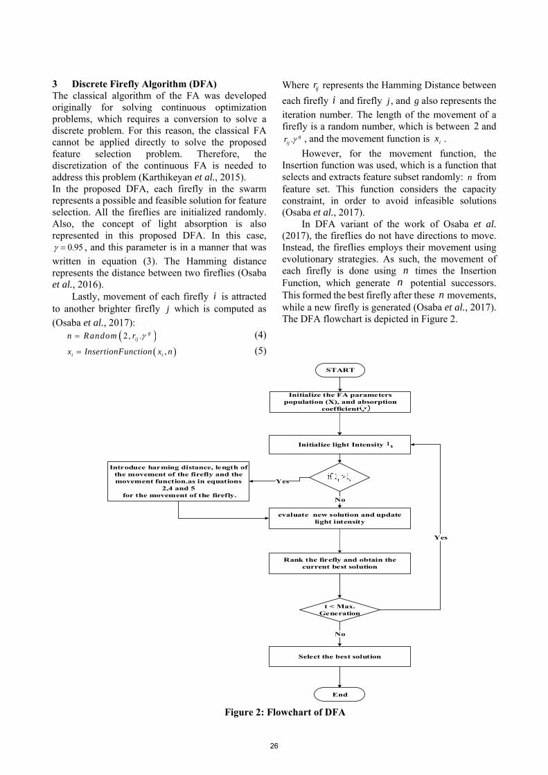
3 Discrete Firefly Algorithm (DFA) The classical algorithm of the FA was developed originally for solving continuous optimization problems, which requires a conversion to solve a discrete problem. For this reason, the classical FA cannot be applied directly to solve the proposed feature selection problem. Therefore, the discretization of the continuous FA is needed to address this problem (Karthikeyan et al., 2015). In the proposed DFA, each firefly in the swarm represents a possible and feasible solution for feature selection. All the fireflies are initialized randomly. Also, the concept of light absorption is also represented in this proposed DFA. In this case,

0.95 , and this parameter is in a manner that was written in equation (3). The Hamming distance represents the distance between two fireflies (Osaba et al., 2016).

Lastly, movement of each firefly i is attracted to another brighter firefly j which is computed as (Osaba et al., 2017):

2, . gijn Random r (4)

,i ix InsertionFunction x n (5)

Where ijr represents the Hamming Distance between

each firefly i and firefly j , and g also represents the iteration number. The length of the movement of a firefly is a random number, which is between 2 and

. gijr , and the movement function is ix .

However, for the movement function, the Insertion function was used, which is a function that selects and extracts feature subset randomly: n from feature set. This function considers the capacity constraint, in order to avoid infeasible solutions (Osaba et al., 2017).

In DFA variant of the work of Osaba et al. (2017), the fireflies do not have directions to move. Instead, the fireflies employs their movement using evolutionary strategies. As such, the movement of each firefly is done using n times the Insertion Function, which generate n potential successors. This formed the best firefly after these n movements, while a new firefly is generated (Osaba et al., 2017). The DFA flowchart is depicted in Figure 2.

START

Initialize the FA parameters population (X), and absorption

coefficient

Initialize light Intensity

Introduce harming distance, length of the movement of the firefly and the movement function.as in equations

2,4 and 5 for the movement of the firefly.

Yes

evaluate new solution and update light intensity

No

Rank the firefly and obtain the current best solution

t < Max. Generation

Select the best solution

No

Yes

End

Figure 2: Flowchart of DFA

26

4 Face Recognition Algorithm In implementing the face recognition system, the steps presented in this section were followed. The first stage was achieved by training the images for detection and extraction which was done using discrete cosine transform (DCT) and Haar wavelet based discrete wavelet transform (DWT), the second stage was achieved also using discrete firefly algorithm (DFA) for feature selection, and finally the last stage involves using nearest neighbor classifier (NNC) for the classification of the images. 4.1 Discrete Cosine Transform (DCT) This technique converts a spatial domain waveform into its constituent components represented by a set of coefficients (El Aroussi et al., 2008). However, it expresses a sequence of data points in terms of a sum of cosine functions oscillating at different frequencies (Jagroop & Josan, 2013). DCT has good performance in compaction efficiency, computationally efficient due to its relation to discrete Fourier transform. Its energy is concentrated on low frequencies for natural images due to the fact that natural images mostly possess low frequency features (El Aroussi et al., 2008). DCT is used in feature extraction for face images to reduce dimensionality and data compression (Jagroop & Josan, 2013). However, DCT is used in both holistic and feature appearance-based approach (El Aroussi et al., 2008). Amongst some common variants of DCT are: type-II DCT, and its inverse, and type-III DCT (IDCT). The feature extraction of DCT usually are of two broad stages: the first stage is applied on the entire image to obtain the coefficient, and the second stage uses some of these features for construction of feature vectors (Dabbaghchian et al., 2010).

DCT coefficients for an M N image which represents a matrix that is 2D is given as (Dabbaghchian et al., 2010):

1 1

0 0

( , )

1 (2 1)( ) ( ) ( , ) cos

2

(2 1) vcos

2

M N

x y

F u v

x uu v f x y

MMN

y

N

(6)

0,1,..., 0,1,...u M v N Where:

10

( ) 21 otherwise

(7)

,F x y is the image intensity function, and

,F U V is the DCT coefficient of a 2D matrix.

Image size of M N matrix for large values of

discriminant coefficients can be estimated as (Dabbaghchian et al., 2010):

11 12 1

221 22

1 2

N

N

M M MN M N

x x x

xx xX

a x x

(8)

4.2 Discrete Wavelet Transform (DWT) Wavelet Transform is a popular tool in computer vision and image processing, for its ability to capture localized time-frequency information of image extraction (Xu & Lee, 2014). Wavelet used in discrete transform comes from the fact that they integrate to zero, wave up and down across the axis.

This property ensures that the data is not over represented. Wavelets are signals which are local in time and scale, and generally have an irregular shape (Dhoriya & Shah, 2014). DWT converts the images starting from the spatial domain to frequency domain where the images are divided by vertical and horizontal lines which could be divided into four parts to represent the first-order of DWT (Kaur & Kaur, 2017). The captured images of the face are signals that are represented in space and time, and can be approximated using the orthogonal basis functions. Wavelets are used for the multi-resolution analysis of the images of the face, in which they provide a means for localization of signals in both frequency and time (Dhoriya & Shah, 2014). Filters in DWT decomposition are designed in such a way that the successive layers of the pyramid include only details not considered by the proceeding level (Kaur & Singh, 2015). The decomposition of the data into different frequency ranges allows the isolation of the components of the frequency that are introduced by intrinsic deformations due to expression variations into certain sub-bands, and considers only sub-bands with most relevant information to better the data (Xu & Lee, 2014). DCT is often used in signal processing to represent a signal, the two dimensional DWT (2D-DWT) of an image is given as (Xu & Lee, 2014):

1

0

1

0

1( , , , ) (x)

2

1( )

m

ix

n

jy

xDWT i j k h f k

z

yf y h

zz

(9)

Where i and j represents the binary scaling power, while k and h are constants of the filters.

4.3 Nearest Neighbor Classifier (NNC) An essential classifier for the face recognition is the nearest neighbor classifier (NNC), which is one of the simplest classifiers that is used by researchers in the

27

recent years to achieve a better classification rate. The aim of NNC is the determination of how close the samples are to the test samples (Kaur, 2012). An image in the test is recognized by assigning to it the label of the closest point in the learning set, in which the distance is measured between the image space (Zhu et al., 2015). The closeness between the data points in the kernel nearest neighbor (KNN) is chosen by the Euclidean distance. Between the pixels in a dataset, a distance is assigned. Euclidean distance is the distance between two pixels. The Euclidean distance is given as (Zhu et al., 2015):

221 1 n nd X , Y x y . ........ x y (10)

This Euclidean distance is by default in a KNN classifier. But the distance between the two features

can be measured based on the one of the distance cosine and correlation (Kaur, 2012). KNN has a lesser execution time and better accuracy compared to other commonly used methods like hidden Markov model, and kernel method suite. It is best for classifying persons based on their images. The NNC does not require learning (since it is memory-based), it can be used even with few examples, it works very well in low dimensions for complex surfaces. However, it is slow in classification and, suffers from the curse of dimensionality (Zhu et al., 2015).

The block diagram of the proposed approach is shown in Figure 3, while Figure 4 shows the flowchart of the face recognition system.

Feature extraction using DCT and DWT

Feature selection using DFA

Recognition using nearest neighbour

classifier

Test Face Image

Figure 3: Steps of the Proposed Approach

28

START

Initialize the FA parameters population (X),and absorption

coefficient

Initialize light Intensity

Introduce harming distance,length of the movement of the firefly and the movement function.as in equation

2, 4, and 5 for the movement of the firefly.

Yes

evaluate new solution and update light intensity

No

Rank the firefly and obtain the current best solution

t < Max. Generation

Select the best solution

No

Yes

End

feature Extraction Using DCT & DWT

Data/Images

Classification Using NNC

Figure 4: Flowchart of the Proposed Face Recognition System

5 Results and Discussions The performance of the discrete firefly (DFA) algorithm was implemented using benchmark face database of Olivetti Research Labs (ORL) now known as AT&T and Yale face database. ORL face database consists of frontal images of 40 persons, which captures variations in illumination, accessories and pose like spectacles. The image of each person contains 10 samples each that were taken against a dark homogeneous background. Facial expressions

with open or closed eyes, spectacles, smiling or not smiling and different environmental variations were captured in the database. The face images size is 92x112 pixels with 256 (8-bit) grey levels per pixel.

It consists of five samples for testing and five samples for training from each person. Figure 5 shows some images of the ORL face database.

29

Figure 5: Obtained Image from ORL Face Database

The face database of Yale consists of 15 persons, and 11 samples of 165 images. The variations in expression like sadness, surprise, happy, normal, wink, sleepy and illumination like right, left and center are captured in the images. The face image size

is 92x112 pixels. It consist of five samples for testing and six

samples for training from each person. This is shown in Figure 6.

Figure 6: Obtained Image from Yale Database

The experiment was performed in MATLAB 2017a simulation environment on a 64-bit OS system, intel ® core ™ 15-3470 CPU@ 3.20GHZ with RAM 8.00GB. The DCT extracts low frequency while the DWT extracts the high frequency features for the feature extraction. The DCT transforms the face images of features from a 10x10 square windows that are from the upper most left corner. Next, all the coefficient of the third level DWT approximation coefficients of Haar wavelets are used in forming the initial feature vector. However, the size of the third level DWT coefficient matrix is 12x14 (i.e. 168), while the feature vector has a total size of 268. The population size of the firefly used in implementing the DFA is 20, and also the maximum number of iterations is 20.

The DFA algorithm, when implemented on

ORL face database, achieved an average recognition accuracy of 97.75%, with a recognition time of 42.27 seconds for fifty runs, and the recognition time/image was 0.21 sec/image. Also, when the DFA algorithm was implemented on Yale face database, it achieved an average recognition accuracy of 89.30% with a recognition time of 40.33 seconds also for fifty runs, and the recognition time/image was 0.54 sec/image.

The proposed DFA algorithm was compared with other meta-heuristic algorithms done by other researchers like Firefly Algorithm (FA), Particle Swarm Optimization (PSO), Genetic Algorithm (GA), and Binary Particle Swarm Optimization (BPSO) Algorithm. The summary of the comparison of the DFA used for feature selection in face recognition with respect to the other algorithms using ORL Face Database is shown in Table 1.

30

Table 1: Comparison of DFA with other Algorithms Using ORL Face Database Authors Year Approach Classifier

Used Recognition

Accuracy Number of Training

Images Used Liu and

Wang (2008) 2008 GA K-NN 90.50% 5

(Cheng et al., 2011)

2011 BPSO Nearest Neighbor

93.25% 5

Darestani et al. (2013)

2013 PSO MLP 90.00% 5

(Agarwal & Bhanot, 2015)

2015 FA Nearest Neighbor

94.38% 5

Proposed DFA

2018 DFA Nearest Neighbor

97.75% 5

Table 1, shows that the DFA algorithm has a better recognition accuracy than the other earlier works that was done on FR. This is due to the fact that some of the optimization techniques used in feature selection of the face recognition are continuous and requires a discrete process, while the face recognition itself is a discrete problem, and the DFA is a discrete algorithm: so employing a discrete algorithm for a discrete problem will provide a higher recognition accuracy.

6 Conclusion This paper presents a discrete firefly algorithm (DFA) based feature selection scheme for face recognition system. Feature selection phase of the face recognition process attempts to obtain the most discriminative features between two or more individuals’ faces to produce the best accuracy in the databases capturing variations in expression or occlusion, illumination and pose. Some of the optimization techniques used for the feature selection are continuous and requires a discrete process. DFA was employed for the feature selection. The DFA was implemented using benchmark face database of Olivetti Research Labs (ORL), now known as AT&T and Yale face database. The DFA gave an average recognition accuracy of 97.75%, with a recognition time of 42.27 seconds on the ORL face database, while the algorithm gave an average recognition accuracy of 89.30% with a recognition time of 40.33 seconds on Yale face database. Future research work should consider employing different discrete algorithms like discrete ant colony optimization (DACO), and discrete bat algorithm (DBA).

Acknowledgement This research work is supported by the Control-and-Computer Research Group of the Department of Computer Engineering, Faculty of Engineering, Ahmadu Bello University, Zaria, Kaduna State Nigeria. Also, the authors will like to thank the anonymous reviewer and the chief Editor, Dr. Abel Usoro, for his insightful comments and suggestions, which have been greatly beneficial for improving the quality of this work. References Agarwal, V., & Bhanot, S. (2015). Firefly Inspired

Feature Selection for Face Recognition. Paper presented at the Eighth International Conference on Contemporary Computing (IC3), 2015 Noida, India.

Angle, S., Bhagtani, R., & Chheda, H. (2005). Biometrics: A Further Echelon of Security. Paper presented at the UAE International Conference on Biological and Medical Physics, UAE, Dubai.

Babatunde, R., Olabiyisi, S., Omidiora, E., & Ganiyu, R. (2015). Local Binary Pattern and Ant Colony Optimization Based Feature Dimensionality Reduction Technique For Face Recognition Systems. British Journal of Mathematics and Computer Science, 11(5), 1-11. doi: 10.9734/BJMCS/2015/19490

Babatunde, R. S., Isiaka, R. M., Adigun, O. J., & Babatunde, A. N. (2017). Implication of Variation in Ant Colony Optimization Algorithm (ACO) Parameters on Feature Subset Size. Computing & Information Systems Journal, 21(3), 1-8.

Bakshi, U., & Singhal, R. (2014). A New Approach of Face Recognition Using DCT PCA and

31

Neural Network in Matlab. International Journal of Emerging Trends & Technology in Computer Science (IJETTCS), 3(3), 238-241.

Bakshi, U., Singhal, R., & Malhotra, M. (2014). Biometric Technology: A Look and Survey at Face Recogntion. International Journal of Engineering Science Invention, 3(6), 24-30.

Boubenna, H., & Lee, D. (2016). Feature Selection for Facial Emotion recognition Based on Genetic Algorithm. Paper presented at the 12th International Conference on Natural Computation, Fuzzy Systems and Knowledge Discovery (ICNC-FSKD), 2016 Changsha, China

Cervante, L., Xue, B., Zhang, M., & Shang, L. (2012). Binary Particle Swarm Optimisation for Feature Selection: A Filter Based Approach. Paper presented at the IEEE Congress on Evolutionary Computation (CEC), 2012, Brisbane, QLD, Australia.

Cheng, G., Shi, C., Zhu, K., & Gong, K. (2011). The Application of Binary Particle Swarm Algorithm in Face Recognition. Paper presented at the Seventh International Conference on Computational Intelligence and Security (CIS), 2011 Hainan, China.

Dabbaghchian, S., Ghaemmaghami, M. P., & Aghagolzadeh, A. (2010). Feature extraction using discrete cosine transform and discrimination power analysis with a face recognition technology. Pattern recognition, 43(4), 1431-1440. doi: https://doi.org/10.1016/j.patcog.2009.11.001

Darestani, M. R. Y., Sheikhan, M., & Khademi, M. (2013). Face Recognition Using Contourlet-Based Features and Hybrid PSO-Neural Model. Paper presented at the 5th Conference on Information and Knowledge Technology (IKT), 2013 Shiraz, Iran

Dhoriya, N. R., & Shah, D. U. (2014). Comparative Study of Compression Techniques and Compressed Image Face Recognition System. International Journal of Engineering Science Invention, 3(5), 39-45.

El Aroussi, M., Amine, A., Ghouzali, S., Rziza, M., & Aboutajdine, D. (2008). Combining DCT and LBP Feature Sets for Efficient Face Recognition. Paper presented at the 3rd International Conference on Information and Communication Technologies: From Theory to Applications, Damascus, Syria

Fernandes, S., & Bala, J. (2017). A Comparative Study on Various State of the Art Face Recognition Techniques under Varying Facial

Expressions. The International Arab Journal of Information Technology, 14(2), 254-259.

Hemalatha, G. L., & Govindan, V. (2015). Feature Selection Using Modified Particle Swarm Optimisation For Face Recognition. International Journal of Research in Engineering and Technology, 4(1).

Jadon, S., Kumar, M., & Rathi, Y. (2015). Face Recognition Using Som Neural Network With Ddct Facial Feature Extraction Techniques. Paper presented at the International Conference on Communications and Signal Processing (ICCSP), 2015 Melmaruvathur, India

Jagroop, R., & Josan, K. (2013). Face Recognition System- A Survey. International Journal of Science and Research (IJSR), 4(1), 2021-2024. doi: SUB15737

Jameel, S. (2015). Face Recognition System Using PCA and DCT in HMM. International Journal of Advanced Research in Computer and Communication Engineering, 4(1), 13-18. doi: DOI 10.17148/IJARCCE.2015.4103

Kallianpur, A. K., Kalyani, A., Naligay, S. E., & Kallimani, J. S. (2016). Facial Recognition Using Discrete ABC. Paper presented at the International Conference on Advances in Computing, Communications and Informatics (ICACCI), 2016 Jaipur, India.

Karthikeyan, S., Asokan, P., Nickolas, S., & Page, T. (2015). A hybrid discrete firefly algorithm for solving multi-objective flexible job shop scheduling problems. International Journal of Bio-Inspired Computation, 7(6), 386-401.

Kaur, H., & Kaur, N. (2017). Review of Image Fusion and its techniques. International Journal of Advanced Research in Computer Science (IJARCS), 8(5).

Kaur, M. (2012). K-Nearest Neighbor Classification Approach for Face and Fingerprint at Feature Level Fusion. International Journal of Computer Applications, 60(14).

Kaur, R., & Singh, E. H. (2015). Review On Image Fusion And Its Techniques. International Journal of Computer Networks and Wireless Communications (IJCNWC), 5(2), 508-515.

Keche, M. J. K., Yeotikar, M. V. K., & Dhore, D. M. P. (2014). Human Face Recognition using Wavelet Transform based Approach. International Journal of Computer & Mathematical Sciences (IJCMS),, 3(9), 2347-8527.

Khan, N., & Gupta, M. (2016). Face Recognition System using Improved Artificial Bee Colony algorithm. Paper presented at the International Conference on Electrical, Electronics, and

32

Optimization Techniques (ICEEOT), 2016, Chennai, India

Liu, N., & Wang, H. (2008). Feature Selection in Frequency Domain and Its Application to Face Recognition. Paper presented at the IEEE International Joint Conference on Neural Networks (IJCNN), 2008, Hong Kong, China.

Lobato, F. S., & Steffen, J. V. (2013). Multi-Objective Optimization Firefly Algorithm Applied to (Bio) Chemical Engineering System Design. American Journal of Applied Mathematics and Statistics, 1(6), 110-116. doi: 10.12691/ajams-1-6-1

Maini, R., & Aggarwal, H. (2009). Study and Comparison of Various Image Edge Detection Techniques. International journal of image processing (IJIP), 3(1), 1-11.

Manikantan, K., Shet, M. S., Patel, M., & Ramachandran, S. (2012). DWT-based Illumination Normalization and Feature Extraction for Enhanced Face Recognition. International Journal of Engineering & Technology, 1(4), 483-504.

Mistry, K., Zhang, L., Neoh, S. C., Lim, C. P., & Fielding, B. (2017a). A Micro-GA Embedded PSO Feature Selection Approach to Intelligent Facial Emotion Recognition. IEEE transactions on cybernetics, 47(6), 1496-1509. doi: 10.1109/TCYB.2016.2549639

Mistry, K., Zhang, L., Sexton, G., Zeng, Y., & He, M. (2017b). Facial Expression Recongition using Firefly-based Feature Optimization. Paper presented at the IEEE Congress on Evolutionary Computation (CEC), 2017 San Sebastian, Spain

Osaba, E., Carballedo, R., Yang, X.-S., & Diaz, F. (2016). An Evolutionary Discrete Firefly Algorithm with Novel Operators for Solving the Vehicle Routing Problem with Time Windows Nature-Inspired Computation in Engineering (pp. 21-41): Springer, Cham.

Osaba, E., Yang, X.-S., Diaz, F., Onieva, E., Masegosa, A. D., & Perallos, A. (2017). A Discrete Firefly Algorithm to Solve a Rich Vehicle Routing Problem Modelling a Newspaper Distribution System with Recycling Policy. Soft Computing, 21(18), 5295-5308. doi: 10.1007/s00500-016-2114-1

Ramadan, R. M., & Abdel-Kader, R. F. (2009). Face Recognition Using Particle Swarm Optimization-Based Selected Features. International Journal of Signal Processing, Image Processing and Pattern Recognition, 2(2), 51-65.

Ruan, C., Ruan, Q., & Li, X. (2010). Real Adaboost Feature Selection for Face Recognition. Paper presented at the IEEE 10th International Conference on Signal Processing (ICSP), 2010 Beijing, China

Saleh, I. A. (2009). Principle Component Selection for Face Recognition Using Neural Network. Reference Journal of Computation and Mathematics, 6(1), 179-191.

Satone, M., & Kharate, G. (2014). Face Recognition Technique Using Pca, Wavelet and Svm. International Journal on Computer Science and Engineering (IJCSE), 6(1), 58-62.

Sawalha, R., & Doush, I. (2012). Face Recognition Using Harmony Search-Based Selected Features. International Journal of Hybrid Information Technology, 5(2), 1-16.

Shivdas, A. E. (2014). Face Recognition Using Artificial Neural Network. International Journal of Research in Management, Science & Technology, (IJRMST), 2(1), 61-65.

Tiwari, V. (2012). Face Recognition Based on Cuckoo Search Algorithm. Indian Journal of Computer Science and Engineering (JJCSE), 3(3), 401-405.

Xu, W., & Lee, E.-J. (2014). Face Recognition Using Wavelets Transform and 2D PCA by SVM Classifier. International Journal of Multimedia and Ubiquitous Engineering, 9(3), 281-290. doi: http://dx.doi.org/10.14257/ijmue.2014.9.3.26

Xue, B., Qin, A. K., & Zhang, M. (2014a). An Archive Based Particle Swarm Optimisation for Feature Selection in Classification. Paper presented at the IEEE Congress on Evolutionary Computation (CEC), 2014, Beijing, China.

Xue, B., Zhang, M., & Browne, W. N. (2014b). Particle swarm optimisation for feature selection in classification: Novel initialisation and updating mechanisms. Applied Soft Computing, 18, 261-276.

Yang, X.-S. (2009). Firefly Algorithms for Multimodal Optimization. Paper presented at the International Symposium on Stochastic Algorithms: Foundations and Applications, SAGA.

Zhou, H., Mian, A., Wei, L., Creighton, D., Hossny, M., & Nahavandi, S. (2014). Recent Advances on Singlemodal and Multimodal Face Recognition: A Survey. IEEE Transactions on Human-Machine Systems, 44(6), 701-716. doi: 10.1109/THMS.2014.2340578

Zhu, N., Xu, T., Wei, L., & Tang, T. (2015). A Nearest Neighbor Classifier Based on Virtual Test Samples for Face Recognition. Optik-International Journal for Light and Electron

33

Optics, 126(21), 2799-2803. doi: http://dx.doi.org/10.1016/j.ijleo.2015.07.014

34

Pilot Contamination Effect Mitigation in Massive Multiple Input Multiple Output

System and Analysis of Mitigation Techniques

*Saidu M. Waziri1, Muhammad B. Abdulrazaq2, Abdoulie M. S. Tekanyi1, Abdullahi Mohammad2 and Hassan A. Abdulkareem1

1Department of Communications Engineering, Ahmadu Bello University, Zaria, Kaduna State, Kaduna, Nigeria 2Department of Computer Engineering, Ahmadu Bello University, Zaria, Kaduna State, Kaduna-Nigeria mw.waziri@gmail.com, mbashiray@yahoo.com, amtekanyi@abu.edu.ng, msabdallah79@gmail.com,

ha2zx@yahoo.com

*Corresponding Author

ABSTRACT Purpose: The aim of this research work is to develop a Pilot Allocation Protocol (PAP) decontamination scheme in order to mitigate the effect of Pilot Contamination (PC) and enhance the performance of cell edge users in Time Division Duplexing (TDD) Massive Multiple-Input Multiple-Output (M-MIMO) systems. Development/Methodology/Approach: A PAP was developed based on sectional pilot sequence sharing and initialization using Rayleigh fading channel. The developed PAP technique was then implemented, which allocated more than one user to share the same orthogonal pilot sequence within a cell and then created intra cell interference between the users sharing the same pilot sequence but suppressed inter cell interference between users sharing the same pilot sequence in other cells and mitigate the effect of PC. Simulation was done in MATLAB/SIMULINK 2016Ra environment. Findings: Simulation results verify the performance improvement of the proposed technique over that of conventional schemes in a typical M-MIMO system, throughout the range (64, 250 and 256) of Base Station (BS) antennas considered for both Uplink (UL) and Downlink (DL), using Zero Forcing (ZF) and Matched Filter (MF) detectors/precoders as signal equalizers. Furthermore, it was evident that ZF has a better Bit Error Rate (BER) performance in comparison with MF. Research Limitation: MF detector/precoder performed poorly in BER analysis when compared with ZF detector/precoder. Originality/Value: The significant contribution of this research work is the development of a PAP based on sectional pilot sequence sharing and initialization using Rayleigh fading channel, considering the allocation protocol.

Keywords: Massive Multiple Input Multiple Output (M-MIMO), Pilot Contamination (PC) and Pilot Allocation Protocol (PAP). Paper Type: Research Paper

1 Introduction Massive Multiple Input Multiple Output (M-MIMO) has been identified as a leading technology to cater for the high data demand rate of the next generation wireless devices also known as 5G. In this technology, large number of antenna arrays concurrently is used to serve many user terminals (UTs), with each UT considered as a single antenna device, in the same time frequency resource (Jose et al., 2009). Asymptotic analysis in accordance with random matrix theory (Elijah et al., 2016) shows that both the intra cell interference and correlated noise can be efficiently mitigated, as the number of Base Station (BS) antennas leans towards boundlessness. Additionally, the energy consumed by cellular BSs can be substantially reduced (Yin et al., 2013).

M-MIMO systems are robust, since failure in one or a few antennas would not significantly affect the general system performance. In addition, optimal performance can be reached by using simple linear processing/detection schemes based on Zero Forcing (ZF) and Matched Filter (MF), when the number of BS antennas inclines toward infinitude. Similar to standard MIMO systems, accurate estimation of the Channel State Information (CSI) of each user is required by the base station and this is done either through reciprocity, that is in Time Division Duplex (TDD) or through feedback method as in Frequency Division Duplex (FDD) schemes (Elijah et al., 2016).

TDD is preferred as the best mode to acquire an accurate estimate of timely CSI in wireless systems in place of FDD due to the fact that the estimation requirement of TDD can be done in one direction and used in both directions as shown in Figure 1, while in

35

FDD estimation and feedback are required for both forward and reverse directions (Guo et al., 2017).

Due to the popularity of FDD among existing networks (3G and 4G), it continues to attract more interest. The TDD scheme depends on the concept of downlink and uplink channels’ reciprocity. It has been considered to be a good choice because the forward channel is assumed to be equal to the transpose of the converse channel and the needed information is gotten from transmitted pilots on the inverse link (de Carvalho, 2014). However, due to shortage in orthogonal pilot sequence and the condensed network deployment, several neighbor cells may use the same pilot sequence (non-orthogonal) and the pilot spots in pilot patterns of the several neighbor cells may super impose, which will directly affect the performance of the system.

Figure 1: Reciprocity in M-MIMO System

This is known as Pilot Contamination (PC) (Vardhan et al., 2016). Furthermore, the conventional use of Matched Filter (MF) and Zero Forcing (ZF) as processing schemes will impose intercell interference on the Down Link (DL) transmission, which cannot be reduced by adding more number of antennas at the BSs. In an effort to address the problem of PC in a multi-cell architecture, different schemes have been proposed.

These schemes are grouped into (1) Pilot-based estimation approach and (2) Sub-space estimation approach (Ngo, 2015). In the pilot-based approach, estimation of the channels of users is done with orthogonal pilot sequence within the cell and non-orthogonal pilot sequence across the cells and this leads to extreme Inter-Cell Interference (ICI) while in the sub-space estimation approach, the channels of users are estimated with limited or no pilot sequence which depends on high order statistical parameters that are susceptible to error in the estimation of user channels.

The rest of the paper is organized into sections. Section two cover the reviews of Massive MIMO System Model and linear estimation techniques. Section three is devoted to detailing the PC problem, the proposed PAP technique is also discussed. In Section four simulation results are presented and

discussed, while in section five we review pilot contamination mitigation techniques with focus on pilot based sub-category. Pilot contamination open issues in massive MIMO are listed and discussed in section six, and lastly section seven concludes the paper.

2 Review of Massive MIMO System Model M-MIMO system consists of a single BS and a single K active user. The BS is furnished with M antennas, while each user is considered as a single antenna device as shown in Figure 2. It is assumed that all K users share the same time-frequency resource and the BS and the UTs have perfect knowledge of the CSI. The channels are learned at the BS and the UTs during the training phase.

Let M KH C be the channel matrix sandwiched between the K UTs and the M BS antenna array, where the thK column of H, denoted

by kh , represents the channel 1M vector linking the

BS and the thK UT, assuming that the elements of H

are identically independent distributed (i.i.d), gaussian distributed with zero mean and unit variance.

Figure 2: Massive MIMO System 2.1 Uplink Transmission Uplink transmission is the process whereby the BS receives signals from KUTs. Let ks , where

2| | 1kS E , be considered as the signal that the

thK UT is transmitted. Since all KUTs share the same

frequencies, the 1M received signal vector at the BS is the summation of all signals emanatting from all KUTs.

1

K

ul u k kk

y h s n

(1)

Where, u is the average signal to noise ratio (SNR),1Mn C 1 is the additive noise vector, and

36

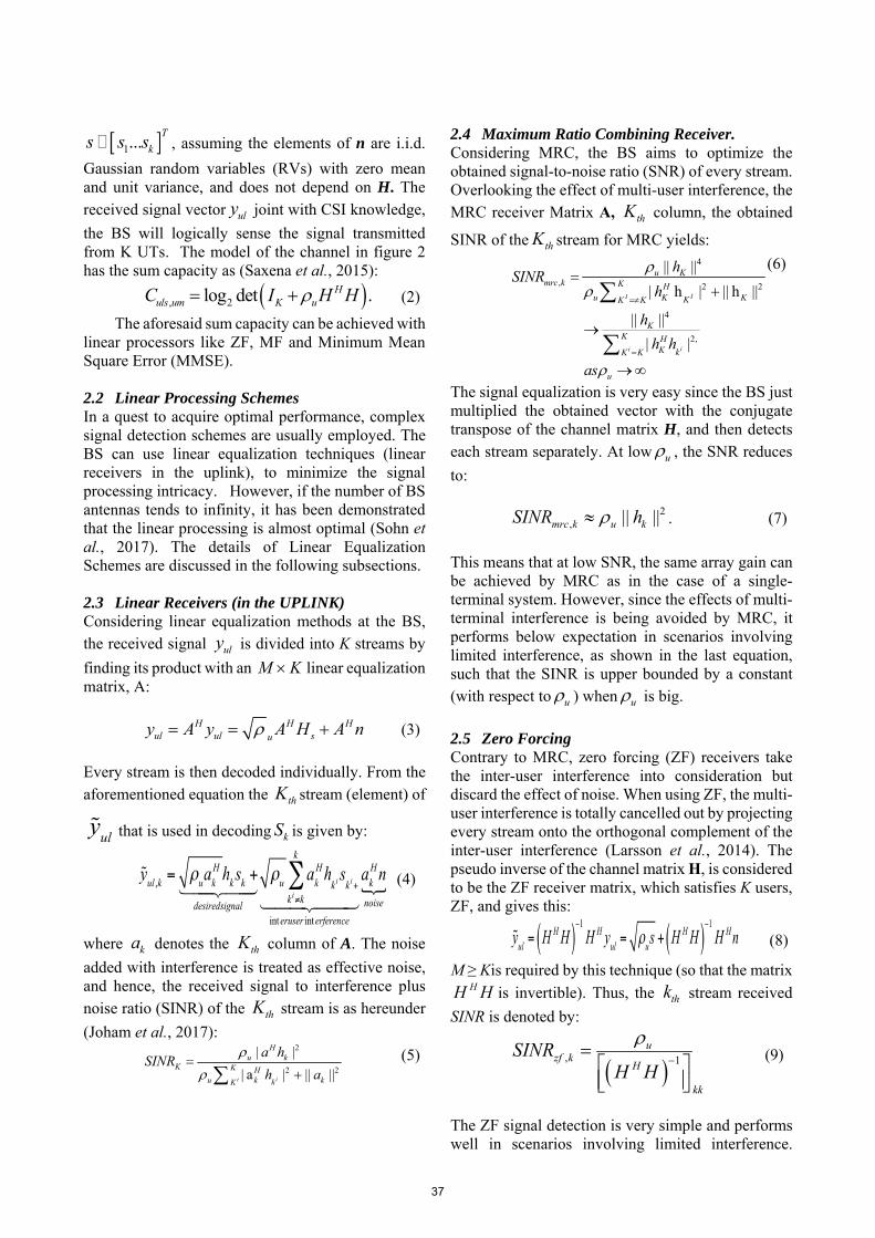
1...T

ks s s , assuming the elements of n are i.i.d.

Gaussian random variables (RVs) with zero mean and unit variance, and does not depend on H. The received signal vector uly

joint with CSI knowledge,

the BS will logically sense the signal transmitted from K UTs. The model of the channel in figure 2 has the sum capacity as (Saxena et al., 2015):

, 2log det .Huls um K uC I H H (2)

The aforesaid sum capacity can be achieved with linear processors like ZF, MF and Minimum Mean Square Error (MMSE).

2.2 Linear Processing Schemes In a quest to acquire optimal performance, complex signal detection schemes are usually employed. The BS can use linear equalization techniques (linear receivers in the uplink), to minimize the signal processing intricacy. However, if the number of BS antennas tends to infinity, it has been demonstrated that the linear processing is almost optimal (Sohn et al., 2017). The details of Linear Equalization Schemes are discussed in the following subsections.

2.3 Linear Receivers (in the UPLINK) Considering linear equalization methods at the BS, the received signal uly

is divided into K streams by

finding its product with an M K linear equalization matrix, A:

H H H

ul ul suy A y A H A n (3)

Every stream is then decoded individually. From the aforementioned equation the thK stream (element) of

that is used in decoding kS is given by:

(4)

where ka denotes the thK column of A. The noise

added with interference is treated as effective noise, and hence, the received signal to interference plus noise ratio (SINR) of the thK

stream is as hereunder

(Joham et al., 2017): 2

2 2

| |

| a | || ||ii

Hu k

K K Hu k kkK

a hSINR

h a

(5)

2.4 Maximum Ratio Combining Receiver. Considering MRC, the BS aims to optimize the obtained signal-to-noise ratio (SNR) of every stream. Overlooking the effect of multi-user interference, the MRC receiver Matrix A, thK column, the obtained

SINR of the thK stream for MRC yields: 4

, 2 2

4

2,

|| ||

| h | || h ||

|| ||

| |

II

ii

u Kmrc k K H

u K KKK K

KK H

K kK K

u

hSINR

h

h

h h

as

(6)

The signal equalization is very easy since the BS just multiplied the obtained vector with the conjugate transpose of the channel matrix H, and then detects each stream separately. At low u , the SNR reduces

to:

2, || ||mrc k u kSINR h . (7)

This means that at low SNR, the same array gain can be achieved by MRC as in the case of a single-terminal system. However, since the effects of multi-terminal interference is being avoided by MRC, it performs below expectation in scenarios involving limited interference, as shown in the last equation, such that the SINR is upper bounded by a constant (with respect to u ) when u is big.

2.5 Zero Forcing Contrary to MRC, zero forcing (ZF) receivers take the inter-user interference into consideration but discard the effect of noise. When using ZF, the multi-user interference is totally cancelled out by projecting every stream onto the orthogonal complement of the inter-user interference (Larsson et al., 2014). The pseudo inverse of the channel matrix H, is considered to be the ZF receiver matrix, which satisfies K users, ZF, and gives this:

(8)

M ≥ Kis required by this technique (so that the matrix HH H is invertible). Thus, the thk stream received

SINR is denoted by:

, 1

uzf k

H

kk

SINRH H

(9)

The ZF signal detection is very simple and performs well in scenarios involving limited interference.

37

Increasing transmit power can achieve a much higher SINR. However, it performs below expectation under noise-limited scenarios. In comparison to MRC, the implementation complexity of ZF is higher because of the computation of the pseudo inverse of the channel gain matrix (Ul mulk, 2015).

3 Pilot Contamination By considering UL training, before the transmitter can send information to the receiver, the receiver sends information to the transmitter at the BS, but the transmitted symbols are known on both sides so that it could train the symbols. Based on this known and properties of its symbols, then the transmitter can estimate the unknown channel vector h added with some noise n of user 1, which leads to the corrupted

version of the right channel vector h of user 1.

Figure 3: Uplink training

However, at the same time there might be a second user (user 2) which also wants to have access to the BS and it also sends training symbols to the BS. If the BS at the transmitter is not aware of this it might happened that it considers the signal coming from the second user (user 2)as part of the original user (user 1), and that will have automatic effect on the downlink when the BS is transmitting data to the first user (user 1). Where h1 is the channel vector of user 2, this effect is called Pilot Contamination (PC), because the interfering part of the channel vector of user 2 (h1) contaminates the channel information of user 1. Multi cell Architecture of M-MIMO system is shown in Figure 4.

We are obliged by pilot contamination to cautiously design pilot mitigationtechniques for a full dimensional MIMO. The aim of this thesis is to assess scenarious under which pilot contamination becomes an important issue in delivering the benefits of M-MIMO system, and study techniques that mitigate its effect.

Figure 4: Multi-Cell Architecture of M-MIMO Farhang et al. (2014) looked into the problem of pilot contamination in cosine modulated multi-tone (CMT) based M-MIMO networks with the view to address the issue. The scheme takes the advantage of the special property of CMT, known as blind equalization property. It was evident that when the technique was extended from single user to a large-scale cellular M-MIMO system, channel estimation error due to (PC) was removed without any coordination among the different base stations or transmission of more training information. Furthermore, it was proved that the proposed solution performed equally good or even better compared to MF. having perfect CSI. Also, the output SINR of the proposed algorithm was observed to have converged towards that of the MMSE solution which has a perfect knowledge of CSI of the various users within its neighboring cells. However, the scheme is highly computationally complex due to the high order statistical parameters needed to estimate the channels and the process could introduce serious error in the channels’ estimation.

A pilot contamination mitigation scheme based on Smart Pilot Assignment (SPA) to enhance the performance of users affected severely by PC was investigated by Zhu et al. (2015). It is done, particularly, by taking into consideration the characteristics of the channels large-scale fading. The base station measures the ICI of the individual training sequences produced from the users having the same training sequence in neighboring cells.

Contrary to the traditional way of allocating training sequences to users haphazardly, the SPA scheme allocates a training sequence that has the least ICI to a user with the poorest channel quality sequentially to enhance its performance. The scheme proves theoretically that the pilot allocation generated by it is the answer to the optimization problem Pi in a greedy way that can approach the novel optimization problem P as the number of antennas tends to infinity. However, the scheme did not break away from the conventional way of

38

initializing all training sequences for the training that leads to the re-use of the same training sequences in the adjacent cells, thereby causing ICI.

Pilot contamination issue in M-MIMO systems, for cell-edge and cell-center user terminals (UTs) was investigated by Zhu et al. (2016). A novel scheme based on soft pilot re-use (SPR) and Multi-Cell Block Diagonalization (MBD) was used to address this issue. It has been established that users at the cell-edge suffer from severe PC than their center-cell counterparts. In view of this development SPR is used in maximizing the quality of service (QoS) of users at the cell edge by re-using a cell-center pilot group for all center-cell users and a cell-edge pilot group for users at the cell edge in the adjacent cells which is determined by their large-scale fading coefficients.

The MBD pre-coding is utilized for a multi-cell scenario, to mitigate ICI and enhanced the QoS for cell-edge users. However, the enhanced rates of the UL and DL throughputs of the proposed scheme was achieved at the expense of a more pilot sequence requirement for channel state information estimation as a tradeoff with resources for data transmission within the coherence interval in comparison to conventional methods and also the scheme is still based on full pilot sequence initialization and reuse of non-orthogonal pilot sequence in different cells in a multi-cell scenario which is the major source of PC.

One of the methods used in Time Division Duplex (TDD) system is collaboration between cells so that they will transmit their pilots at different times and therefore there will be no inter-cell interference from non-orthogonal pilots. This is found to be difficult as synchronizing different levels of the network (micro-, nano-, and pico-cells), and possibly many cells, will be a huge task. Another suggestion is to randomly change the orthogonal code of pilots so that the interfering signals will randomly change and therefore will have averaging rather than summing effect.

However, because the random change will happen only once in a coherent time, the interference is bound to remain from the same sources for a significantly long time. We therefore suggest an approach that investigate rather than letting the interference to come from neighboring cells that have the same orthogonal pilots. We can make them come from the same cell in order to avoid coordination among neighboring to reduce processing complexity. This can be done by grouping a number of user terminals (UT) and letting them use the same orthogonal pilot. This means the cell in which the interfering UTs belong to has total control of all the interfering UTs and at the same time needs no

communication to any other cell to control the interference.

A stream of known previously agreed upon pilot bits from the receiver and or transmitter can be used to estimate the channel state information (CSI). Because of the grouping of many UTs, it means the orthogonal pilots can now be more available to go round the network. Fixed orthogonal channels can be assigned to each cell (pilot reuse > 1) which will be assigned to UTs on demand. Motivated by the concept of pilot reuse and Soft Pilot Reuse (SPR) particularly, which allocates orthogonal pilot sequence to cell-edge users, we therefore proposed Pilot Allocation Protocol (PAP) decontamination scheme operating in TDD mode to mitigate the effect of PC in M-MIMO system. This technique is based on sectional pilot sequence initialization and sharing with a pilot sequence reuse factor of 1/3, which can allocate more than one user to share same orthogonal pilot sequence within a cell which then creates Intra Cell Interference and mitigates the effect of PC. However, this is achieved by separating the users using distinct codes unique to each of the interfering users.

We found out that the scheme performed best among the discussed techniques in terms of average cell throughput. In this scheme the orthogonal pilot sequences are divided into 3 groups and allocated to three different cells. That is to say that within each cell and at least the next neighboring cells the pilot sequences are orthogonal to each other. So, when orthogonal pilot sequences within a particular group are exhausted by users, then sharing starts. This is done between users, which then creates an intra cell interference among the users sharing the same pilot sequence, and again are then made orthogonal to each other by employing a property of hadamard matrix. The matrix assigns distinct codes to the interfering users sharing the same pilot sequence in each coherence interval as against discarding or queuing the users for the next available pilot sequence in the conventional technique.

The concept mitigates the effect of pilot contamination to a large extent and also increases the number of users that of the available resources without increasing the number of the orthogonal pilot sequences. Figure 5 depicts the multi-cell architecture of the developed PAP technique.

Figure 5 shows the pilot sequence allocation and sharing pattern of the developed PAP scheme based on sectional initialization and pilot sequence sharing between users.

39

Figure 5: PAP Technique Each color in Figure 5 represents a particular

group (a section) of the total orthogonal pilot sequences while cells having the same colors use the same type of orthogonal pilot sequences with a minimum reuse distance of one kilometer since the cell radius considered is 500 m. Furthermore the green, blue and red colored signals emanating from the user equipments to the base stations represent the individual pilot sequences in each cell.

Users transmitting same color of signals are sharing the same pilot sequence but then are separated using distinct signs of hardmad matrix. The broken signals in blue colors represent interfering signals from far cells and they formed part of the additive white gaussian noise.

The following methodology was adopted to carry out the research work:

a) A TDD M-MIMO channel model with a varying number of base station antennas, number of users per cell, and power of user equipment were developed based on Rayleigh fading channel taking into consideration pilot allocation protocol. PAP was implemented based on sectional initialization and pilot sequence sharing, which allocates pilot sequence to many users within a cell and their training was conducted using different codes.

b) Users were grouped into cell center and cell edge in accordance with their large-scale fading coefficient.

c) A signal detection scheme based on matched filter and zero forcing, for equalizing the signals was implemented.

d) The UL Signal to Interference plus Noise Ratio (SINR) of users at the cell edge was then calculated and the average UL cell throughput determined.

e) The DL Signal to Interference plus Noise

Ratio (SINR) of users at the cell edge was then calculated and the average UL cell throughput determined.

f) Validation of the results was done by

comparing the results gotten from the Pilot Allocation Protocol (PAP) technique and that of conventional schemes in terms of average uplink cell throughput and bit error rate as performance metrics.

4 Results of the Simulation The PAP simulation results obtained using simulation parameters highlighted in Table 1were plotted for the PAP technique Zero Forcing (ZF) and Matched Filter (MF) linear detectors.

Figure 6: Average Uplink Cell Throughput against Number of BS Antennas for the two

Schemes with ZF

Figure 6 shows the average Uplink (UL) cell Throughput against the Number of Base Station (BS) Antennas for the developed PAP and conventional schemes all with ZF detector, with number of BS antennas ranging from 60 to 256 antennas and 50% of the bandwidth for data transmission allocated to UL data transmission.

From the simulation results in Figure 6, when the number of BS antennas is at 64, the conventional schemes offer an average UL throughput of 31 b/s/Hz while the developed PAP offers an average UL cell throughput of 33

40

than the conventional scheme when ZF detector was used.

Table 1: Model Parameters used

Parameters Units Number of cells LTotal 19 Number of antenna in BS M 32 ≤ M ≤ 256 Number of users in the ith cell Ki 32

Number of pilot resource Kcs 10 Cell radius R 500m Average transmit power at users ρp ρu

10dbm

Average transmit power at BS ρd 12dbm

Pathloss exponent α 3 Log normal shadowing fading σshow

8db

Carrier frequency 2GHz System bandwidth 10MHz Minimum distance between user and BS

30m

At 250 BS antennas, the conventional scheme offers an average cell throughput of 37 b/s/Hz while the developed PAP offers an average UL cell throughput of 57.5 b/s/Hz, which is 20.5 b/s/Hz more than the conventional scheme. This shows that the performance improvement of the interfering users (cell edge) users of the developed PAP schemes is better than that of the conventional scheme as the number of BS antennas increases.

It can be observed that when the number of BS antennas was set at 256 the conventional scheme offers an average cell throughput of 37.5 b/s/Hz while the developed PAP offers an average UL cell throughput of 58 b/s/Hz, which is 20.5 b/s/Hz more than the conventional scheme. The PAP scheme outperforms the conventional scheme and hence further proves that the performance improvement of the interfering users (cell edge users) of the PAP technique is better than that of the conventional scheme as the number of BS antennas increases.

Figure 7 shows the Average Uplink Cell Throughput against the Number of Base Station (BS) antennas for the developed PAP and conventional scheme all with MF detector, with number of BS antennas ranging from 60 to 256 BS antennas and 50% of the bandwidth for data transmission allocated to UL data transmission. From simulation results in Figure 7, when the number of BS antennas is at 64, the conventional scheme offers an average UL throughput of 24 b/s/Hz while the developed PAP offers an average UL cell throughput of 25.5 b/s/Hz improvement, which is 1.5 b/s/Hz

more than the conventional scheme when MF detector was used.

Figure 7: Average Uplink Cell Throughput against Number of BS Antennas for the two

Schemes with ZF

At 250 BS antennas the conventional scheme offers an average cell throughput of 34.5 b/s/Hz while the developed PAP offers an average UL cell throughput of 42.5 b/s/Hz, which is 8 b/s/Hz more than the conventional scheme. At 256 BS antennas the conventional scheme offers an average cell throughput of 34.5 b/s/Hz while the developed PAP offers an average UL cell throughput of 43 b/s/Hz which is 8.5 b/s/Hz more than the conventional method. This shows that the performance improvement of the interfering users (cell edge) users of the developed PAP schemes is better than that of the conventional scheme as the number of BS antennas increases with MF detector. Similarly, the PAP simulation results obtained using simulation parameters highlighted in Table 1 were plotted for the PAP technique using Zero Forcing (ZF) and Matched Filter (MF) linear precoders.

From simulation results in Figure 8, when the number of BS antennas is at 64, the conventional scheme offers an average DL throughput of 31 b/s/Hz while the developed PAP offers an average DL cell throughput of 33 b/s/Hz improvement, which is 2 b/s/Hz more than the conventional scheme when ZF detector was used. At 250 BS antennas the conventional scheme offers an average cell throughput of 37.5 b/s/Hz while the developed PAP offers an average DL cell throughput of 57 b/s/Hz, which is 20.5 b/s/Hz more than the conventional scheme. This shows that the performance improvement of the interfering users (cell edge users)

41

of the developed PAP schemes is better than that of the conventional scheme as the number of BS antennas increase.

Figure 8: Average Downlink Cell Throughput

against Number of BS Antennas for the two Schemes with ZF

It can be seen that when the number of BS

antennas was set at 256 the conventional schemes offer an average DL cell throughput of 37.5 b/s/Hz while the developed PAP offers an average DL cell throughput of 58 b/s/Hz, which is 20.5 b/s/Hz more than the conventional scheme. The PAP scheme outperforms the conventional scheme and hence further proved that the performance improvement of the interfering users (cell edge users) of the PAP is better than that of the conventional scheme as the number of BS antennas increase.

Figure 9: Average Downlink Cell Throughput against Number of BS Antennas for the two

Schemes with MF

Figure 9 shows the Average Downlink (DL) Cell Throughput against the Number of Base Station (BS)

antennas for the developed PAP and conventional scheme all with MF precoder, with number of BS antennas ranging from 60 to 256 antennas and 50% of the bandwidth for data transmission allocated to DL data transmission. From simulation results in Figure 9, when the number of BS antennas is at 64, the conventional scheme offers an average DL throughput of 24 b/s/Hz while the developed PAP offers an average DL cell throughput of 25.5 b/s/Hz improvement, which is 1.5 b/s/Hz more than the conventional scheme when MF detector was used.

At 250 BS antennas the conventional scheme offers an average cell throughput of 34.5 b/s/Hz while the developed PAP offers an average DL cell throughput of 42.5 b/s/Hz, which is 8 b/s/Hz more than the conventional scheme. At 256 BS antennas the conventional scheme offers an average cell throughput of 34.5 b/s/Hz while the developed PAP offers an average DL cell throughput of 43 b/s/Hz this shows that the performance improvement of the interfering users (cell edge users) of the developed PAP schemes is better than that of the conventional scheme as the number of BS antennas increase.

It can be seen that when the number of BS antennas was set at 256 the PAP scheme outperforms the conventional scheme and hence further proved that the performance improvement of the interfering users (cell users) of the PAP is better than that of the conventional technique as the number of BS antennas keep increasing with MF detector.

Figure 10: A plot of BER Performance for the PAP Scheme with ZF

42

It can be observed from Figure 10 that as the SNR increases the BER also decreases and the developed PAP using ZF for UL met the BER requirement for audio signal that is10-3 of BER in digital communications at SNR of 8 dB, which means in every 1000 bit you have 1 error.

Figure 11: A plot of BER Performance for the

PAP Scheme with ZF

It can be observed from Figure 11 that as the SNR increases the BER also decreases and the developed PAP using ZF for DL met the BER requirement for audio signal that is 10-3 of BER in digital communications at SNR of 8 dB, which means in every 1000 bit you have 1 error

Figure 12: A plot of BER Performance for

the PAP Scheme with MF

It can be observed from Figure 12 that the developed PAP using MF for UL attained a BER of 10-1.25 = 1/101.25 = 1/17.8 = 1/18, which means

in every 18 bits of transmission you have 1 error, at SNR of 8 db.

Figure 13: A plot of BER Performance for

the PAP Scheme with MF

Figure 13 shows the DL Bit Error Rate performance of the developed PAP model using MF. It can be observed from Figure 15 that the developed PAP using MF for DL attained a BER of 10-1.25 = 1/101.25 = 1/17.8 = 1/18, which means in every 18 bits of transmission you have 1 error, at SNR of 8 dB. From the simulation results obtained from the developed PAP scheme using the ZF and MF detection/precoding schemes evaluated at 64,250 and 256 BS antennas, the average cell throughput improvement of the developed PAP scheme outperforms that of the traditional scheme.

The improvement occurred as a result of the pilot sequence allocation protocol adopted by the PAP technique and the way the interfering users (cell edge users) were efficiently separated after sharing of pilot sequence occurs between users. The PAP scheme creates intracell interference and suppressed the effect of Intercell Interference ICI to a large extent which is the major cause of Pilot Contamination during Uplink pilot transmission.

Furthermore, it is important to notice that the average cell throughput improvement performance of the PAP technique is better than that of the conventional scheme with both ZF and MF detection/precoding schemes throughout the range of BS antennas considered (64,250 and 256). This is due to the fact that in the PAP technique pilot, sequence of users within and across the neighboring cells were made to be orthogonal to each other and when sharing occurs (when pilot sequence of users was made to be non-orthogonal) to each other, codes were used to separate the interfering users throughout the length of the coherence interval.

43

5 Mitigation Techniques 5.1 Pilot Open Loop Control The path loss and transmit power of a User Terminal (UT) is determined by the average obtained power of a pilot sequence at the base station (BS). Usually terminals located close to the BS have a less pathloss and a higher signal power while those located at the edge of the cell usually have a higher pathloss and therefore a lower signal power (Ul mulk, 2015).

This means those terminals near the BS benefit from a reduced pathloss, leading to a better Signal to Interference plus Noise Ratio (SINR). The three different scenarios of pilot reuse at cell edge, close to serving BS and by close cell edge terminals, are described in figure 14 (Saxena et al., 2015). Figure 14 depicts Pilot Reuse at Cell Edge, Pilot Reuse Close to Serving BS and Pilot Reuse by Close Edge Terminals.

(a) Pilot Reuse at Cell Edge and close to BS

(b) Pilot Reuse Close to Serving BS.

(c) Pilot Reuse by Close Edge Terminals.

Figure 14: Uplink Transmission with all Users

Transmitting at Maximum Power Source: Saxena et al. (2015)

5.2 Less aggressive pilot reuse Maximum pilot reuse prompts most extreme inter-cell interference (ICI) when estimating a channel, which can be reduced by using a soft pilot reuse factor (Saxena et al., 2015). Pilot reuse is analogous to the traditional frequency reuse in the sense that user terminals within the pilot reuse area can utilize just a little amount of the time frequency resources during the channel estimation phase (Zhang, 2015). On the other hand, in the case of maximum pilot

repetition, each terminal is permitted to use all the available resources for communication for the rest of the coherence interval which led to less throughput (Sohn et al., 2017). The pilot repetition factor of 1/U is the rate at which pilot resources may be repeated within the network, where U is the quantity of cells that are allotted orthogonal pilot sequence.

Using reuse factor of U>1 mitigates the pilot contamination effect by allotting orthogonal pilot sequence to the surrounding cells leading to huge throughput. The total number of unique time frequency elements earmarked to transmit pilot are KU, where K is the quantity of terminals per cell. The trivial case of pilot repetition is aggressive pilot reuse with U = 1, considering some reserved K time-frequency indices for pilot sequence. The indices may be found any place inside the resource block without loss of simplification. K orthogonal pilot symbols are generated including these indices that are shared randomly at arbitrary or algorithmically within the terminals per cell.

Since the cells are taken to be synchronized, the symbols’ transmissions are synchronized crosswise over cells also. Considering a hexagonal cellular architecture, the minimum reuse factor that can ensure orthogonal pilots in adjacent cells is 1/3. The resources used to implement this reuse factor will triple the number of terminals, that is 3K. A pilot group is allocated to each cell in accordance with the reuse pattern and the users are assigned with the pilots as in the case of maximum pilot reuse. Clearly, a higher value of U will eliminate Pilot Contamination (PC) but at an expense of more training overheads added by using the pilot resources, thereby reducing the resources available for data within a coherence interval (Saxena et al., 2015).

The enhanced estimates are used for better forward and reverse links beamforming at the BS using spatial multiplexing to serve the users. Hence there is a tradeoff between the exact beamforming and transmission of the data afterwards. Figure 16 depicts full pilot reuse and 1/3 pilot reuse respectively (Ul mulk, 2015). Alternatively, there is another technique called Soft Pilot Reuse (SPR) that mitigates PC by allocating more orthogonal pilot sequences to terminals at the cell-edge to improve their Signal to Noise Ratio (SNR). 6 Open Issues While massive MIMO reduces many conventional issues in communication theory less applicable, it reveals entirely fresh challenges that require research, among which are discussed hereunder:

44

6.1 Training Overhead There is need to figure out if the sub-space method can achieve enough CSI quality needed for the pilot-based approach with the same target SINR (Jose et al., 2009). Furthermore, the sub-space techniques need more schemes or information to distinguish the particular eigen vector that corresponds to which user and the assumption that all desired channels are more influential than all interfering channels does not hold in practical system always (Larsson et al., 2014). 6.2 Deployment Scenario Studies are required to investigate the influence of pilot contamination, by considering a more realistic channel model for large MIMO system by bearing in mind statistical channel properties, particularly the spatial-temporal frequency correlation properties and large-scale fading role (Elijah et al., 2016). 6.3 Computational Complexity and Cost There is need for a soft complex pre-coding schemes and CE techniques. While some of the suggested schemes to reduce pilot contamination theoretically sound promising, there is a need to assess their performance by bearing in mind the compromise between its complexity and accuracy (Atzeni et al., 2015). 7 Conclusion Pilot Contamination (PC) is considered as the major drawback of Time Division Duplexing (TDD) Massive Multiple-Input Multiple-Output (M-MIMO) systems because it limits their expected capacity. Several mitigation techniques such as Eigenvalue Decomposition, Cooperative Bayesian Channel Estimation, Blind Equalization Technique, Time Staggering Pilot, and Smart Pilot Assignment have been proposed in literature to address the issue of PC.

This research work focused on Pilot-based estimation category. In the pilot-based method, channels of users are estimated by means of orthogonal pilot sequences within the cell and non-orthogonal pilot (the same pilot) sequences across the cells. However, this technique is largely affected by Intercell Interference (ICI) which is the major cause of Pilot Contamination during UL pilot sequence transmission.

Therefore, we developed a Pilot Allocation Protocol (PAP) decontamination scheme for TDD mode M-MIMO system based on sectional pilot sequence initialization and sharing which allocates more than one user to share the same orthogonal pilot sequence within a cell which then creates Intra Cell Interference, suppresses Inter Cell Interference (ICI) and mitigates the effect of PC among the interfering

User Terminals (UTs). Additionally we reviewed pilot contamination mitigation techniques with focus on pilot based sub-category. Open challenges on pilot contamination in massive MIMO were also digested. Acknowledgment This research work is supported by the Communication-and-Electronic Research Group of the Department of Communications Engineering, Faculty of Engineering, Ahmadu Bello University, Zaria, Kaduna State, Kaduna, Nigeria References Atzeni, I., Arnau, J., & Debbah, M. (2015). Fractional

pilot reuse in massive MIMO systems. Paper presented at the Communication Workshop (ICCW), 2015 IEEE International Conference on.

de Carvalho, E. (2014). Pilot decontamination through pilot sequence hopping in massive MIMO systems. Paper presented at the Global Communications Conference (GLOBECOM), 2014 IEEE.

Elijah, O., Leow, C. Y., Rahman, T. A., Nunoo, S., & Iliya, S. Z. (2016). A comprehensive survey of pilot contamination in massive MIMO—5G system. IEEE Communications Surveys & Tutorials, 18(2), 905-923.

Guo, X., Zhang, J., Chen, S., Mu, X., & Hanzo, L. (2017). Two-Stage Time-Domain Pilot Contamination Elimination in Large-Scale Multiple-Antenna Aided and TDD Based OFDM Systems. IEEE Access.

Joham, M., Neumann, D., & Utschick, W. (2017). Strategies to Combat Pilot Contamination in Massive MIMO Systems. 2nd International Workshop on Challenges and Trends of Broadband Wireless Mobile Access Networks — Beyond LTE-A, 1-44. Retrieved from

Jose, J., Ashikhmin, A., Marzetta, T. L., & Vishwanath, S. (2009). Pilot contamination problem in multi-cell TDD systems. Paper presented at the Information Theory, 2009. ISIT 2009. IEEE International Symposium on, Seoul, South Korea.

Larsson, E. G., Edfors, O., Tufvesson, F., & Marzetta, T. L. (2014). Massive MIMO for next generation wireless systems. IEEE Communications Magazine, 52(2), 186-195.

Ngo, H. Q. (2015). Massive MIMO: Fundamentals and system designs (Vol. 1642): Linköping University Electronic Press.

Saxena, V., Fodor, G., & Karipidis, E. (2015). Mitigating pilot contamination by pilot reuse and power control schemes for massive MIMO

45

systems. Paper presented at the Vehicular Technology Conference (VTC Spring), 2015 IEEE 81st.

Sohn, J.-Y., Yoon, S. W., & Moon, J. (2017). On Reusing Pilots Among Interfering Cells in Massive MIMO. IEEE Transactions on Wireless Communications, 16(12), 8092-8104.

Ul mulk, Z. (2015). Analysis of Pilot Contamination in Very Large Scale MIMO Systems. Department of Electrical Engineering A thesis submitted in partial fulfillment of the requirements for the degree of Masters in Electrical Engineering (MS EE-TCN) In School of Electrical Engineering and Computer Science, National University of Sciences and Technology.

Vardhan, P., Gupta, M., & Kumar, A. (2016). Massive-MIMO-Past, Present and Future: A Review. Indian Journal of Science and Technology, 9(48), 1-13. doi: 10.17485/ijst/2016/v9i48/99891

Yin, H., Gesbert, D., Filippou, M., & Liu, Y. (2013). A coordinated approach to channel estimation in large-scale multiple-antenna systems. IEEE Journal on selected areas in communications, 31(2), 264-273.

Zhang, C. (2015). Fractional Pilot Reuse in Massive MIMO System. IEICE Transactions on Fundamentals of Electronics, Communications and Computer Sciences, 98(11), 2356-2359.

46

Table of Contents Vol 23, No 2, 2019

Methodology for Image Cryptosystem Based on a Gray Code Number System

Babatunde Akinbowale Nathaniel ....................................................................................................................1

A Secured and Energy Efficient Wireless Sensor Networks (WSN) Utilizing CRT-Based Forwarding Technique

Kamaldeen Ayodele Raji and Kazeem Alagbe Gbolagade .............................................................................11

Discrete Firefly Algorithm Based Feature Selection Scheme for Improved Face Recognition

Shittu S. Danraka, Sani M. Yahaya, Aliyu D. Usman, Abubakar Umar and Ahmed M. Abubakar..............23

Pilot Contamination Effect Mitigation in Massive Multiple Input Multiple Output System and Analysis of Mitigation Techniques

Saidu M. Waziri, Muhammad B. Abdulrazaq, Abdoulie M. S. Tekanyi,

Abdullahi Mohammad and Hassan A. Abdulkareem ......................................................................................35

Printed by Printing Services, University of the West of ScotlandUniversity of the West of Scotland is a registered Scottish charity. Charity number SC002520