computer vision lecture 18
TRANSCRIPT
Perc
eptu
al
and S
enso
ry A
ugm
ente
d C
om
puti
ng
Co
mp
ute
r V
isio
n W
S 1
6/1
7
Computer Vision – Lecture 18
Camera Calibration & 3D Reconstruction
18.01.2017
Bastian Leibe
RWTH Aachen
http://www.vision.rwth-aachen.de
Perc
eptu
al
and S
enso
ry A
ugm
ente
d C
om
puti
ng
Co
mp
ute
r V
isio
n W
S 1
6/1
7
Course Outline
• Image Processing Basics
• Segmentation & Grouping
• Object Recognition
• Local Features & Matching
• Object Categorization
• 3D Reconstruction
Epipolar Geometry and Stereo Basics
Camera calibration & Uncalibrated Reconstruction
Structure-from-Motion
• Motion and Tracking
3

Perc
eptu
al
and S
enso
ry A
ugm
ente
d C
om
puti
ng
Co
mp
ute
r V
isio
n W
S 1
5/1
6
Recap: What Is Stereo Vision?
• Generic problem formulation: given several images of
the same object or scene, compute a representation of
its 3D shape
4B. LeibeSlide credit: Svetlana Lazebnik, Steve Seitz
Perc
eptu
al
and S
enso
ry A
ugm
ente
d C
om
puti
ng
Co
mp
ute
r V
isio
n W
S 1
5/1
6
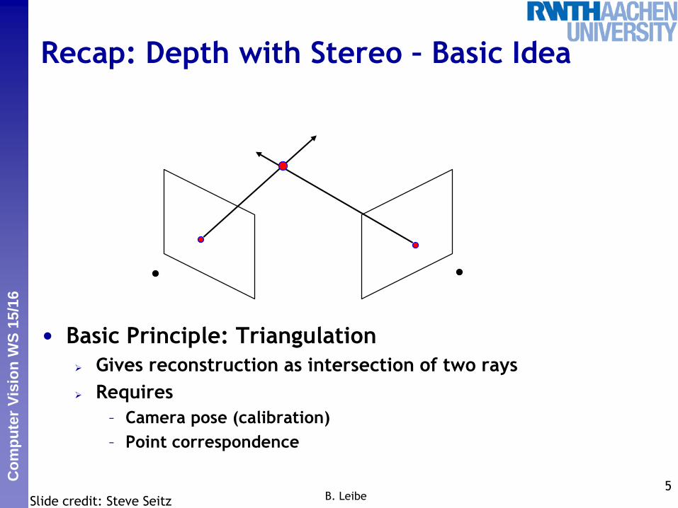
Recap: Depth with Stereo – Basic Idea
• Basic Principle: Triangulation
Gives reconstruction as intersection of two rays
Requires
– Camera pose (calibration)
– Point correspondence
5B. LeibeSlide credit: Steve Seitz
Perc
eptu
al
and S
enso
ry A
ugm
ente
d C
om
puti
ng
Co
mp
ute
r V
isio
n W
S 1
5/1
6
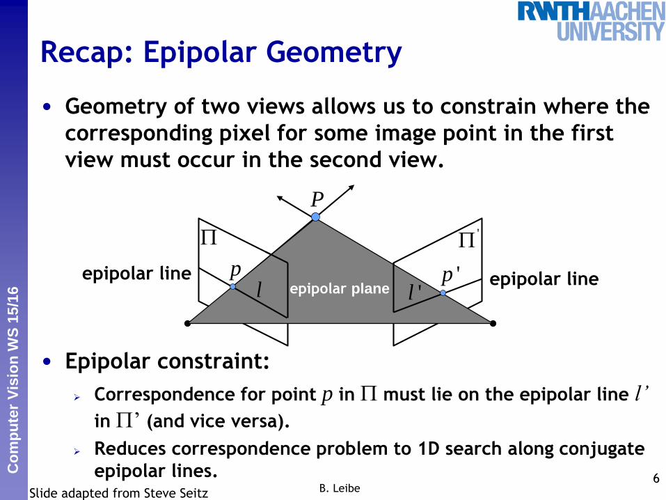
Recap: Epipolar Geometry
• Geometry of two views allows us to constrain where the
corresponding pixel for some image point in the first
view must occur in the second view.
• Epipolar constraint:
Correspondence for point p in must lie on the epipolar line l’
in ’ (and vice versa).
Reduces correspondence problem to 1D search along conjugate
epipolar lines. 6B. Leibe
epipolar planeepipolar lineepipolar line
Slide adapted from Steve Seitz
'
p
P
'pl 'l
Perc
eptu
al
and S
enso
ry A
ugm
ente
d C
om
puti
ng
Co
mp
ute
r V
isio
n W
S 1
5/1
6
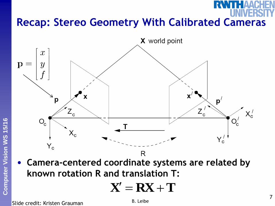
Recap: Stereo Geometry With Calibrated Cameras
• Camera-centered coordinate systems are related by
known rotation R and translation T:
7B. LeibeSlide credit: Kristen Grauman
TRXX

Perc
eptu
al
and S
enso
ry A
ugm
ente
d C
om
puti
ng
Co
mp
ute
r V
isio
n W
S 1
5/1
6
Recap: Essential Matrix
• This holds for the rays p and p’ that
are parallel to the camera-centered
position vectors X and X’, so we have:
• E is called the essential matrix, which relates
corresponding image points [Longuet-Higgins 1981]8
B. Leibe
0 RXTX
0 RXTX x
Let RTE x
0 EXXT
0Epp'T
Slide credit: Kristen Grauman
Perc
eptu
al
and S
enso
ry A
ugm
ente
d C
om
puti
ng
Co
mp
ute
r V
isio
n W
S 1
5/1
6
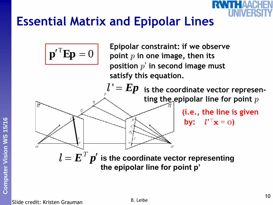
Essential Matrix and Epipolar Lines
10B. Leibe
is the coordinate vector representing
the epipolar line for point p’
is the coordinate vector represen-
ting the epipolar line for point p
0EppEpipolar constraint: if we observe
point p in one image, then its
position p’ in second image must
satisfy this equation.
Slide credit: Kristen Grauman
T E pl
' Epl
(i.e., the line is given
by: l’>x = 0)
Perc
eptu
al
and S
enso
ry A
ugm
ente
d C
om
puti
ng
Co
mp
ute
r V
isio
n W
S 1
5/1
6
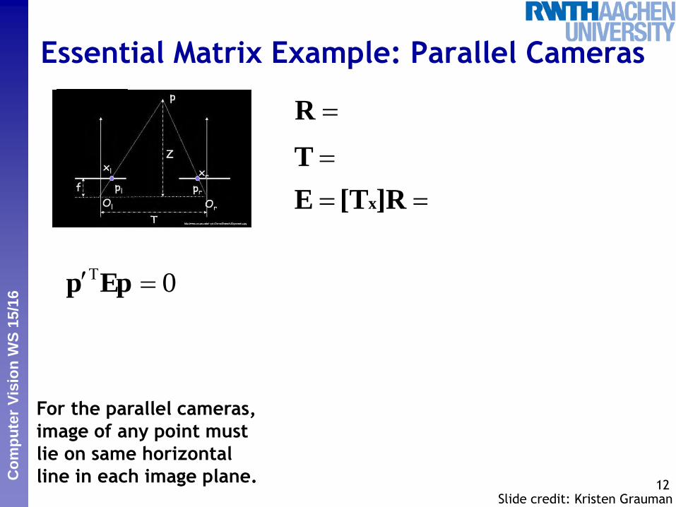
Essential Matrix Example: Parallel Cameras
12
]R[TE
T
IR
x
]0,0,[ d0 0 0
0 0 d
0 –d 0
0Epp
For the parallel cameras,
image of any point must
lie on same horizontal
line in each image plane.Slide credit: Kristen Grauman
Perc
eptu
al
and S
enso
ry A
ugm
ente
d C
om
puti
ng
Co
mp
ute
r V
isio
n W
S 1
5/1
6
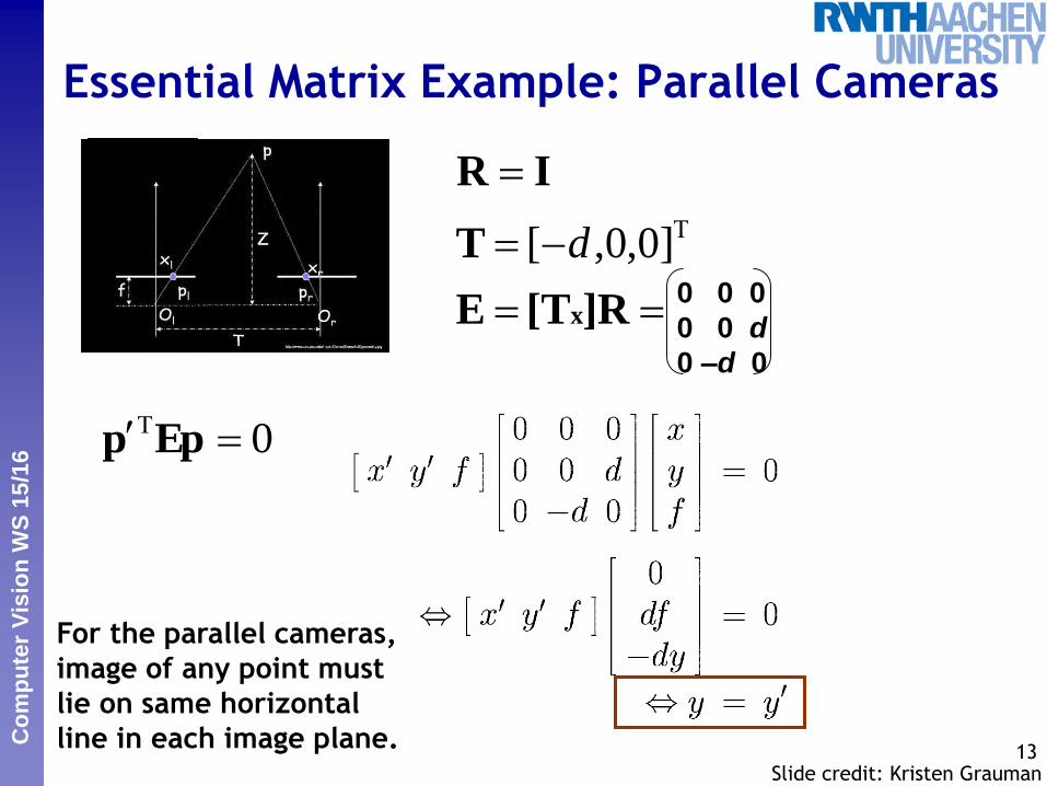
Essential Matrix Example: Parallel Cameras
13
]R[TE
T
IR
x
]0,0,[ d0 0 0
0 0 d
0 –d 0
0Epp
For the parallel cameras,
image of any point must
lie on same horizontal
line in each image plane.Slide credit: Kristen Grauman
Perc
eptu
al
and S
enso
ry A
ugm
ente
d C
om
puti
ng
Co
mp
ute
r V
isio
n W
S 1
5/1
6
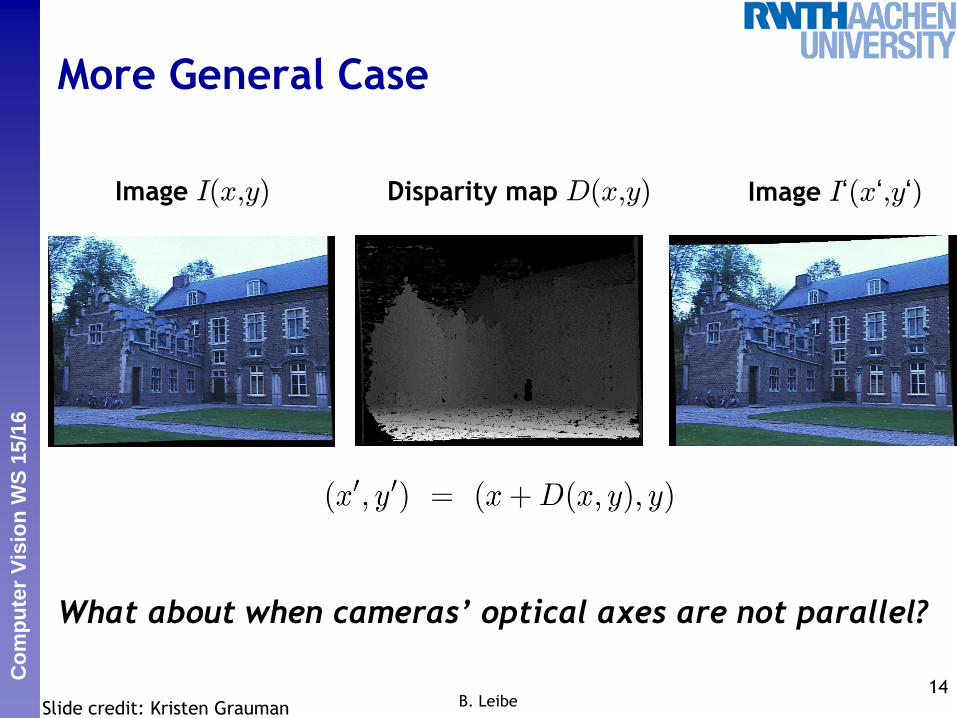
What about when cameras’ optical axes are not parallel?
More General Case
14B. LeibeSlide credit: Kristen Grauman
Image I(x,y) Image I‘(x‘,y‘)Disparity map D(x,y)
Perc
eptu
al
and S
enso
ry A
ugm
ente
d C
om
puti
ng
Co
mp
ute
r V
isio
n W
S 1
5/1
6
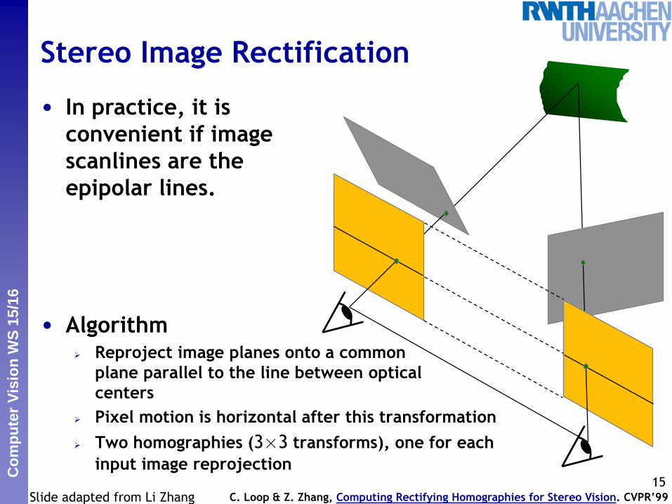
Stereo Image Rectification
• In practice, it is
convenient if image
scanlines are the
epipolar lines.
• Algorithm Reproject image planes onto a common
plane parallel to the line between optical
centers
Pixel motion is horizontal after this transformation
Two homographies (3£3 transforms), one for each
input image reprojection15
C. Loop & Z. Zhang, Computing Rectifying Homographies for Stereo Vision. CVPR’99Slide adapted from Li Zhang
Perc
eptu
al
and S
enso
ry A
ugm
ente
d C
om
puti
ng
Co
mp
ute
r V
isio
n W
S 1
5/1
6
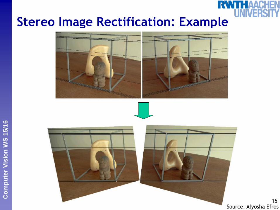
Stereo Image Rectification: Example
16B. Leibe Source: Alyosha Efros
Perc
eptu
al
and S
enso
ry A
ugm
ente
d C
om
puti
ng
Co
mp
ute
r V
isio
n W
S 1
5/1
6
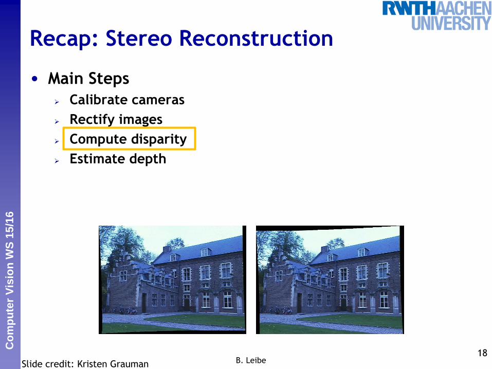
Recap: Stereo Reconstruction
• Main Steps
Calibrate cameras
Rectify images
Compute disparity
Estimate depth
18B. LeibeSlide credit: Kristen Grauman
Perc
eptu
al
and S
enso
ry A
ugm
ente
d C
om
puti
ng
Co
mp
ute
r V
isio
n W
S 1
5/1
6
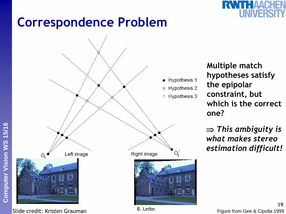
Correspondence Problem
19B. Leibe
Multiple match
hypotheses satisfy
the epipolar
constraint, but
which is the correct
one?
Figure from Gee & Cipolla 1999Slide credit: Kristen Grauman
This ambiguity is
what makes stereo
estimation difficult!
Perc
eptu
al
and S
enso
ry A
ugm
ente
d C
om
puti
ng
Co
mp
ute
r V
isio
n W
S 1
5/1
6
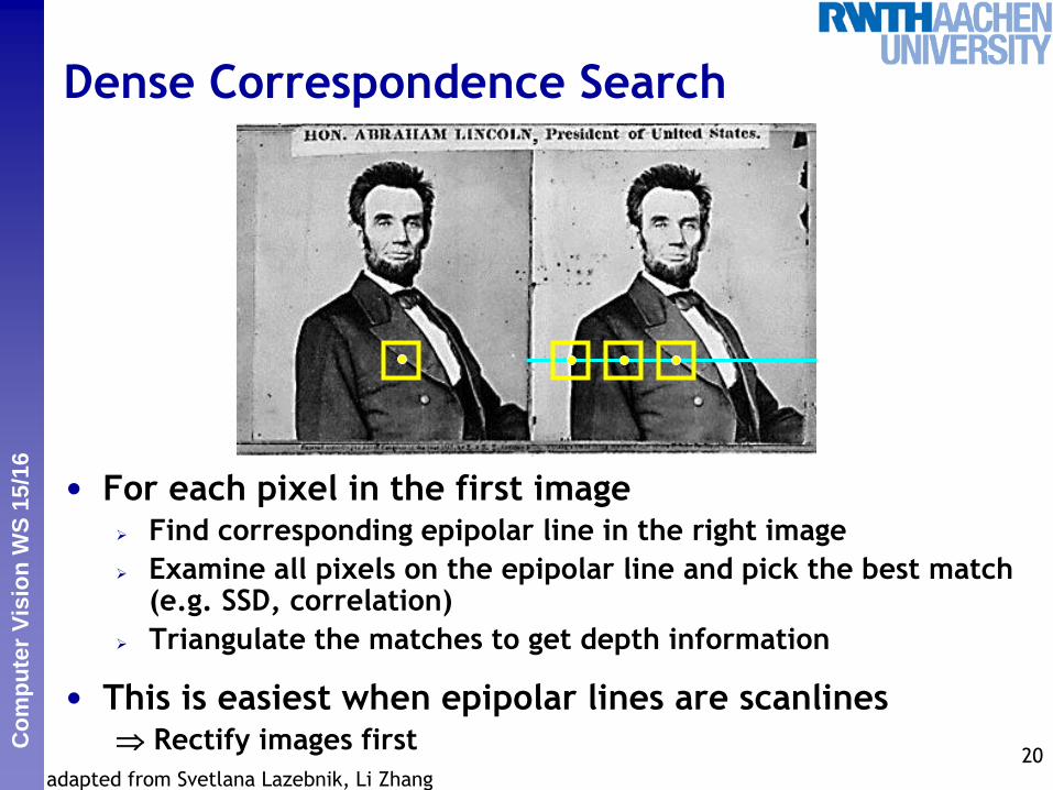
Dense Correspondence Search
• For each pixel in the first image Find corresponding epipolar line in the right image
Examine all pixels on the epipolar line and pick the best match(e.g. SSD, correlation)
Triangulate the matches to get depth information
• This is easiest when epipolar lines are scanlines Rectify images first
20adapted from Svetlana Lazebnik, Li Zhang

Perc
eptu
al
and S
enso
ry A
ugm
ente
d C
om
puti
ng
Co
mp
ute
r V
isio
n W
S 1
5/1
6
Example: Window Search
• Data from University of Tsukuba
21B. LeibeSlide credit: Kristen Grauman

Perc
eptu
al
and S
enso
ry A
ugm
ente
d C
om
puti
ng
Co
mp
ute
r V
isio
n W
S 1
5/1
6
Example: Window Search
• Data from University of Tsukuba
22B. LeibeSlide credit: Kristen Grauman

Perc
eptu
al
and S
enso
ry A
ugm
ente
d C
om
puti
ng
Co
mp
ute
r V
isio
n W
S 1
5/1
6
Effect of Window Size
23B. Leibe
W = 3 W = 20
Want window large enough to have sufficient intensity
variation, yet small enough to contain only pixels with
about the same disparity.
Figures from Li ZhangSlide credit: Kristen Grauman

Perc
eptu
al
and S
enso
ry A
ugm
ente
d C
om
puti
ng
Co
mp
ute
r V
isio
n W
S 1
5/1
6
Alternative: Sparse Correspondence Search
• Idea:
Restrict search to sparse set of detected features
Rather than pixel values (or lists of pixel values) use feature
descriptor and an associated feature distance
Still narrow search further by epipolar geometry
24B. Leibe
What would make good features?Slide credit: Kristen Grauman
Perc
eptu
al
and S
enso
ry A
ugm
ente
d C
om
puti
ng
Co
mp
ute
r V
isio
n W
S 1
5/1
6
Dense vs. Sparse
• Sparse Efficiency
Can have more reliable feature matches, less sensitive to illumination than raw pixels
But… – Have to know enough to pick good features
– Sparse information
• Dense Simple process
More depth estimates, can be useful for surface reconstruction
But… – Breaks down in textureless regions anyway
– Raw pixel distances can be brittle
– Not good with very different viewpoints 25Slide credit: Kristen Grauman
Perc
eptu
al
and S
enso
ry A
ugm
ente
d C
om
puti
ng
Co
mp
ute
r V
isio
n W
S 1
5/1
6
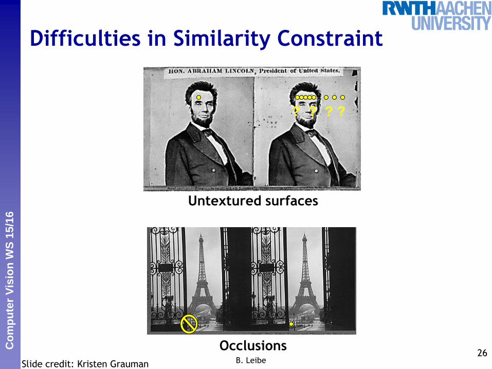
Difficulties in Similarity Constraint
26B. Leibe
Untextured surfaces
????
Occlusions
Slide credit: Kristen Grauman

Perc
eptu
al
and S
enso
ry A
ugm
ente
d C
om
puti
ng
Co
mp
ute
r V
isio
n W
S 1
5/1
6
Summary: Stereo Reconstruction
• Main Steps
Calibrate cameras
Rectify images
Compute disparity
Estimate depth
• So far, we have only considered
calibrated cameras…
• Today
Uncalibrated cameras
Camera parameters
Revisiting epipolar geometry
Robust fitting28
B. LeibeSlide credit: Kristen Grauman
Perc
eptu
al
and S
enso
ry A
ugm
ente
d C
om
puti
ng
Co
mp
ute
r V
isio
n W
S 1
5/1
6
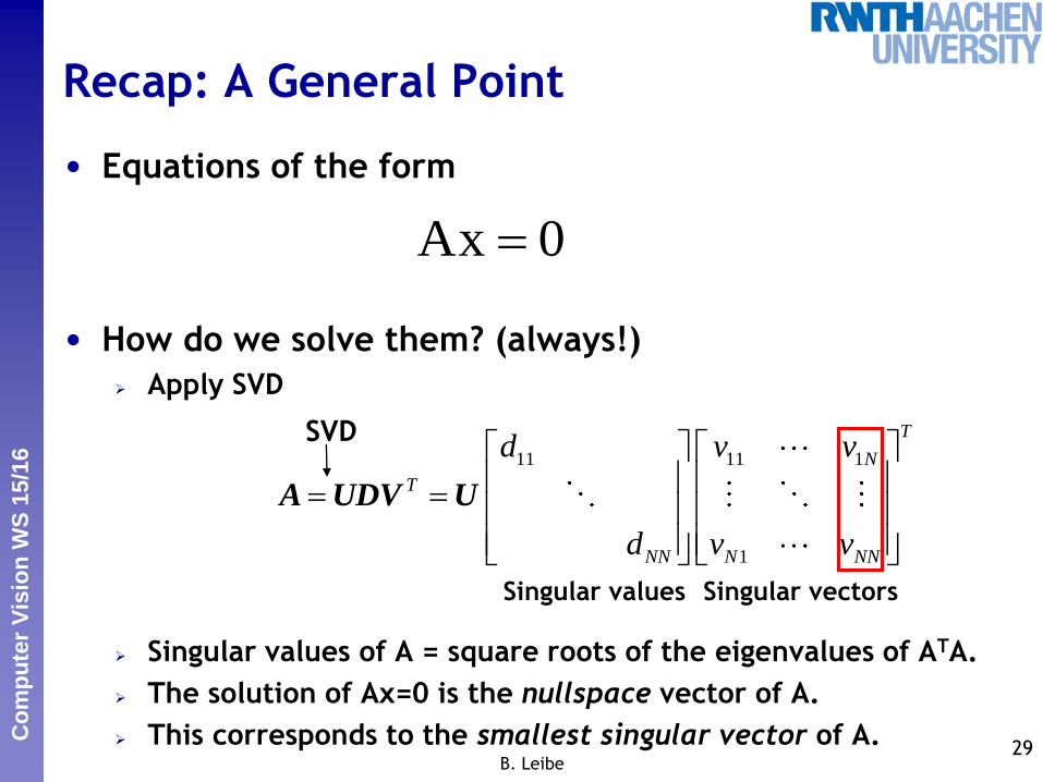
Recap: A General Point
• Equations of the form
• How do we solve them? (always!)
Apply SVD
Singular values of A = square roots of the eigenvalues of ATA.
The solution of Ax=0 is the nullspace vector of A.
This corresponds to the smallest singular vector of A.29
Ax 0
11 11 1
1
T
N
T
NN N NN
d v v
d v v
A UDV U
SVD
Singular values Singular vectors
B. Leibe
Perc
eptu
al
and S
enso
ry A
ugm
ente
d C
om
puti
ng
Co
mp
ute
r V
isio
n W
S 1
5/1
6
Topics of This Lecture
• Camera Calibration Camera parameters
Calibration procedure
• Revisiting Epipolar Geometry Triangulation
Calibrated case: Essential matrix
Uncalibrated case: Fundamental matrix
Weak calibration
Epipolar Transfer
• Active Stereo Laser scanning
Kinect sensor
30B. Leibe
Perc
eptu
al
and S
enso
ry A
ugm
ente
d C
om
puti
ng
Co
mp
ute
r V
isio
n W
S 1
5/1
6
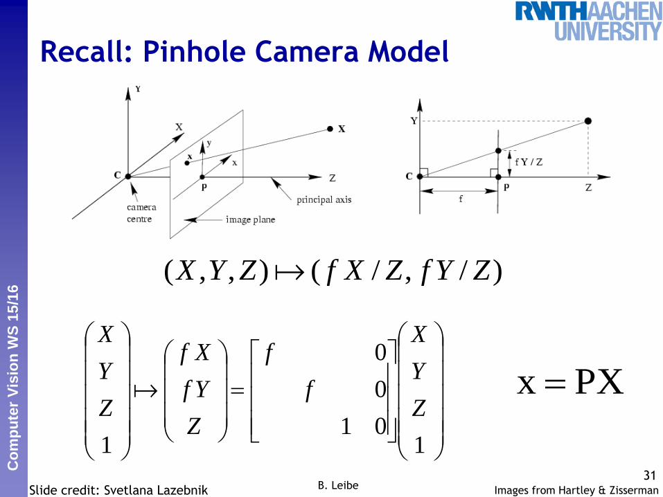
Recall: Pinhole Camera Model
31B. Leibe
)/,/(),,( ZYfZXfZYX
101
0
0
1
Z
Y
X
f
f
Z
Yf
Xf
Z
Y
X
PXx
Slide credit: Svetlana Lazebnik Images from Hartley & Zisserman
Perc
eptu
al
and S
enso
ry A
ugm
ente
d C
om
puti
ng
Co
mp
ute
r V
isio
n W
S 1
5/1
6
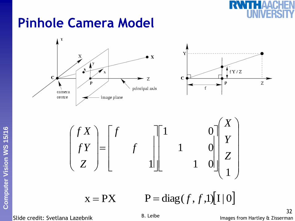
Pinhole Camera Model
32B. Leibe
101
01
01
1Z
Y
X
f
f
Z
Yf
Xf
PXx 0|I)1,,(diagP ff
Slide credit: Svetlana Lazebnik Images from Hartley & Zisserman
Perc
eptu
al
and S
enso
ry A
ugm
ente
d C
om
puti
ng
Co
mp
ute
r V
isio
n W
S 1
5/1
6
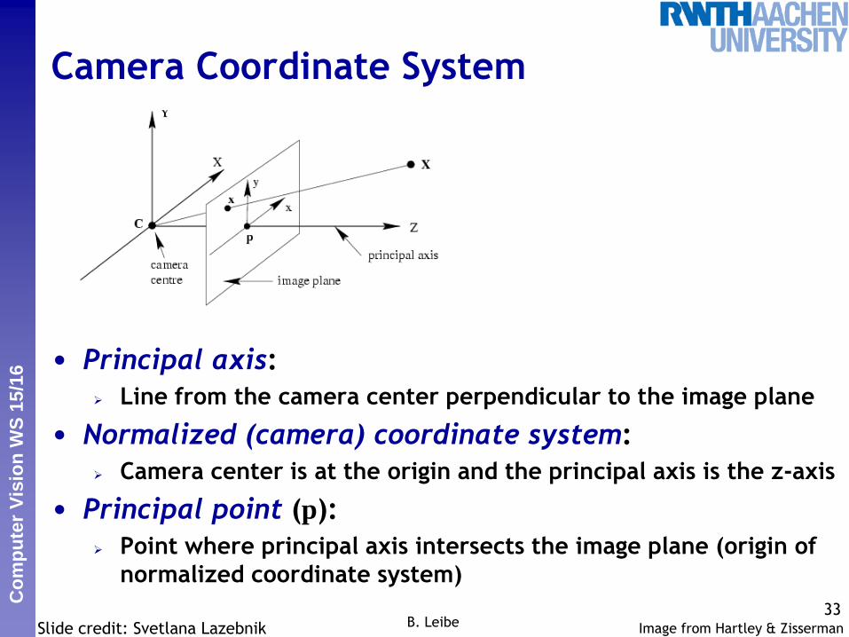
Camera Coordinate System
• Principal axis:
Line from the camera center perpendicular to the image plane
• Normalized (camera) coordinate system:
Camera center is at the origin and the principal axis is the z-axis
• Principal point (p):
Point where principal axis intersects the image plane (origin of
normalized coordinate system)
33B. LeibeSlide credit: Svetlana Lazebnik Image from Hartley & Zisserman

Perc
eptu
al
and S
enso
ry A
ugm
ente
d C
om
puti
ng
Co
mp
ute
r V
isio
n W
S 1
5/1
6
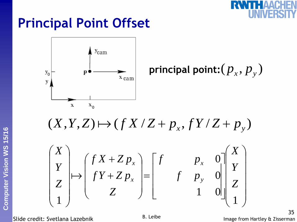
Principal Point Offset
• Camera coordinate system: origin at the principal point
• Image coordinate system: origin is in the corner
34B. Leibe
principal point: ),( yx pp
Slide credit: Svetlana Lazebnik Image from Hartley & Zisserman
Perc
eptu
al
and S
enso
ry A
ugm
ente
d C
om
puti
ng
Co
mp
ute
r V
isio
n W
S 1
5/1
6
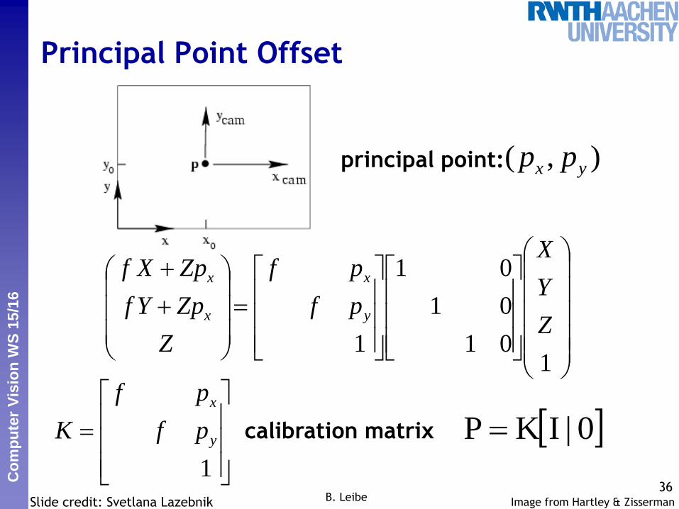
Principal Point Offset
35B. Leibe
principal point: ),( yx pp
Slide credit: Svetlana Lazebnik
)/,/(),,( yx pZYfpZXfZYX
101
0
0
1
Z
Y
X
pf
pf
Z
pZYf
pZXf
Z
Y
X
y
x
x
x
Image from Hartley & Zisserman
Perc
eptu
al
and S
enso
ry A
ugm
ente
d C
om
puti
ng
Co
mp
ute
r V
isio
n W
S 1
5/1
6
Principal Point Offset
36B. Leibe
principal point: ),( yx pp
Slide credit: Svetlana Lazebnik
101
01
01
1Z
Y
X
pf
pf
Z
ZpYf
ZpXf
y
x
x
x
1
y
x
pf
pf
K calibration matrix 0|IKP
Image from Hartley & Zisserman
Perc
eptu
al
and S
enso
ry A
ugm
ente
d C
om
puti
ng
Co
mp
ute
r V
isio
n W
S 1
5/1
6
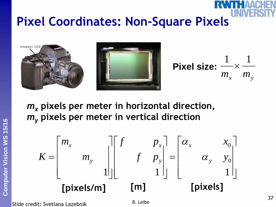
Pixel Coordinates: Non-Square Pixels
mx pixels per meter in horizontal direction,
my pixels per meter in vertical direction
37B. Leibe
0
0
1 1 1
x x x
y y y
m f p x
K m f p y
Pixel size: yx mm
11
[pixels/m] [m] [pixels]
Slide credit: Svetlana Lazebnik
Perc
eptu
al
and S
enso
ry A
ugm
ente
d C
om
puti
ng
Co
mp
ute
r V
isio
n W
S 1
5/1
6
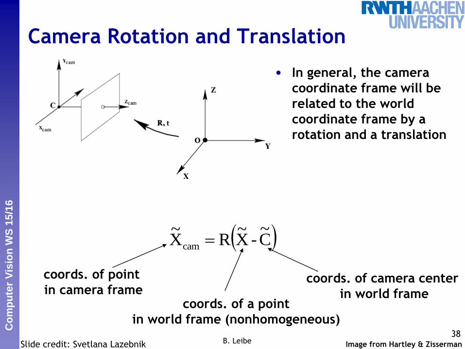
Camera Rotation and Translation
• In general, the camera
coordinate frame will be
related to the world
coordinate frame by a
rotation and a translation
38B. Leibe
C~
-X~
RX~
cam
coords. of point
in camera framecoords. of camera center
in world framecoords. of a point
in world frame (nonhomogeneous)
Image from Hartley & ZissermanSlide credit: Svetlana Lazebnik
Perc
eptu
al
and S
enso
ry A
ugm
ente
d C
om
puti
ng
Co
mp
ute
r V
isio
n W
S 1
5/1
6
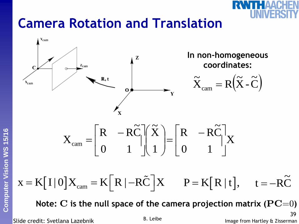
Camera Rotation and Translation
39B. Leibe Image from Hartley & ZissermanSlide credit: Svetlana Lazebnik
C~
-X~
RX~
cam
X10
C~
RR
1
X~
10
C~
RRXcam
camx K I | 0 X K R | RC X P K R | t , C~
Rt
In non-homogeneous
coordinates:
Note: C is the null space of the camera projection matrix (PC=0)

Perc
eptu
al
and S
enso
ry A
ugm
ente
d C
om
puti
ng
Co
mp
ute
r V
isio
n W
S 1
5/1
6
Summary: Camera Parameters
• Intrinsic parameters
Principal point coordinates
Focal length
Pixel magnification factors
Skew (non-rectangular pixels)
Radial distortion
40B. Leibe
0
0
1 1 1
x x x
y y y
m f p x
K m f p y
s s
Slide credit: Svetlana Lazebnik
Perc
eptu
al
and S
enso
ry A
ugm
ente
d C
om
puti
ng
Co
mp
ute
r V
isio
n W
S 1
5/1
6
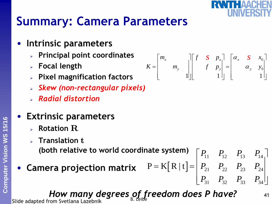
Summary: Camera Parameters
• Intrinsic parameters
Principal point coordinates
Focal length
Pixel magnification factors
Skew (non-rectangular pixels)
Radial distortion
• Extrinsic parameters
Rotation R
Translation t
(both relative to world coordinate system)
• Camera projection matrix
How many degrees of freedom does P have? 41B. Leibe
0
0
1 1 1
x x x
y y y
m f p x
K m f p y
s s
Slide adapted from Svetlana Lazebnik
11 12 13 14
21 22 23 24
31 32 33 34
P K R | t
P P P P
P P P P
P P P P
Perc
eptu
al
and S
enso
ry A
ugm
ente
d C
om
puti
ng
Co
mp
ute
r V
isio
n W
S 1
5/1
6
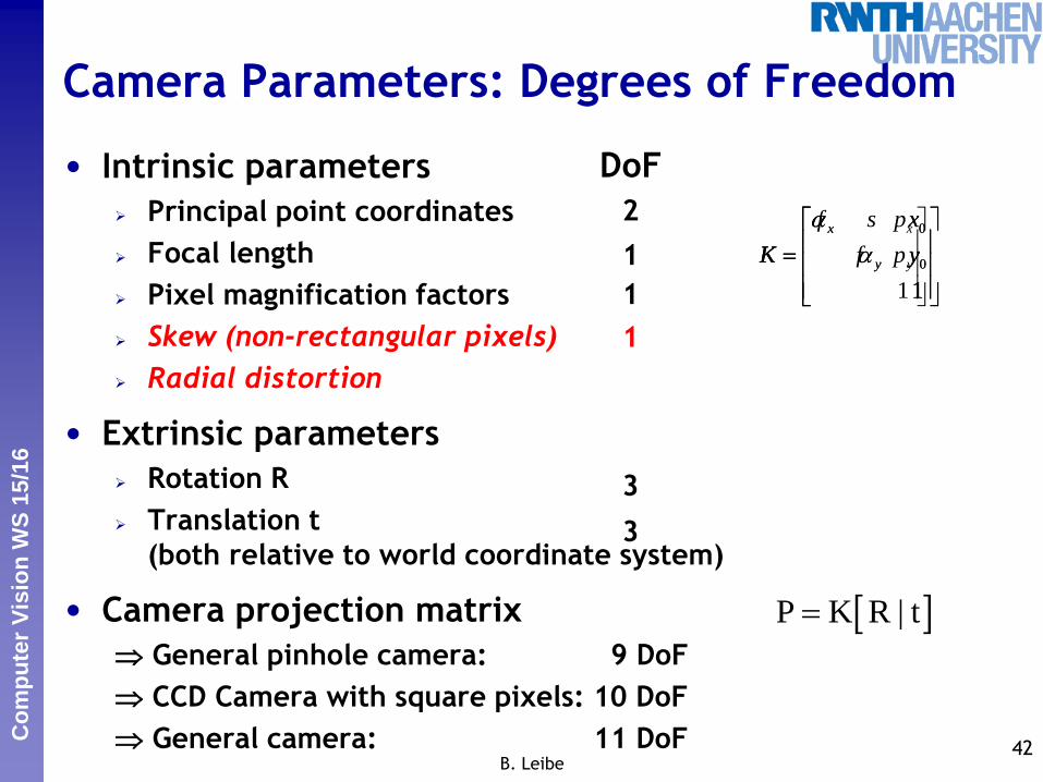
Camera Parameters: Degrees of Freedom
• Intrinsic parameters
Principal point coordinates
Focal length
Pixel magnification factors
Skew (non-rectangular pixels)
Radial distortion
• Extrinsic parameters
Rotation R
Translation t
(both relative to world coordinate system)
• Camera projection matrix
General pinhole camera: 9 DoF
CCD Camera with square pixels: 10 DoF
General camera: 11 DoF 42B. Leibe
0
0
1
x
y
s x
K y
2
1
1
1
DoF
0
0
1
x
y
x
K y
1
x
y
f p
K f p
P K R | t
3
3
Perc
eptu
al
and S
enso
ry A
ugm
ente
d C
om
puti
ng
Co
mp
ute
r V
isio
n W
S 1
5/1
6
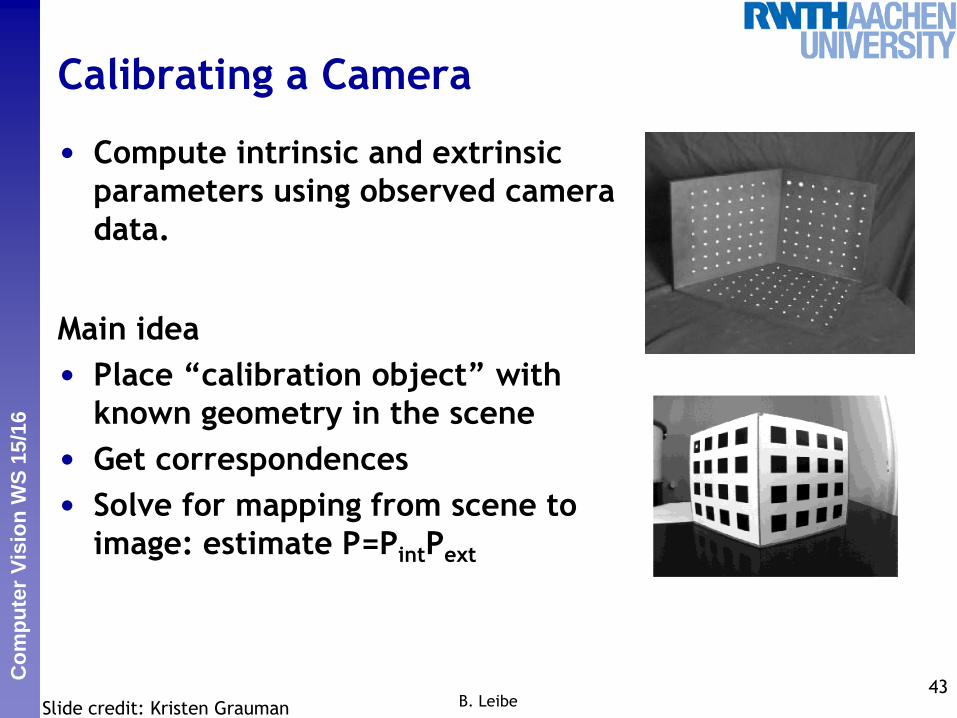
Calibrating a Camera
• Compute intrinsic and extrinsic
parameters using observed camera
data.
Main idea
• Place “calibration object” with
known geometry in the scene
• Get correspondences
• Solve for mapping from scene to
image: estimate P=PintPext
43B. LeibeSlide credit: Kristen Grauman
Perc
eptu
al
and S
enso
ry A
ugm
ente
d C
om
puti
ng
Co
mp
ute
r V
isio
n W
S 1
5/1
6
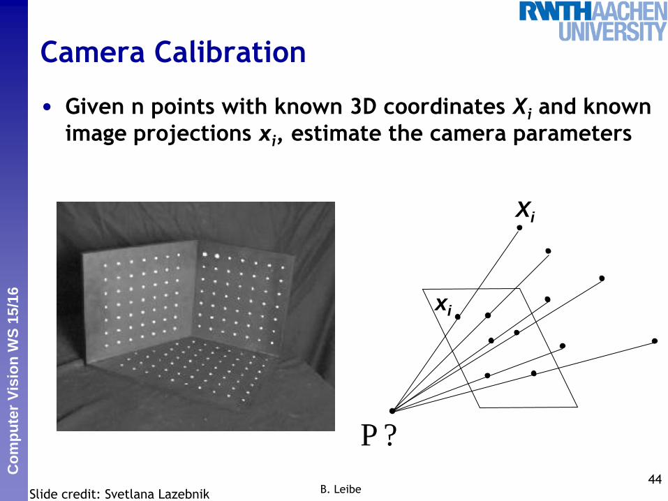
Camera Calibration
• Given n points with known 3D coordinates Xi and known
image projections xi, estimate the camera parameters
44B. Leibe
? P
Xi
xi
Slide credit: Svetlana Lazebnik
Perc
eptu
al
and S
enso
ry A
ugm
ente
d C
om
puti
ng
Co
mp
ute
r V
isio
n W
S 1
5/1
6
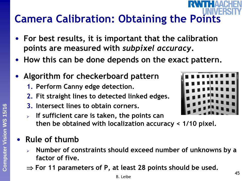
Camera Calibration: Obtaining the Points
• For best results, it is important that the calibration
points are measured with subpixel accuracy.
• How this can be done depends on the exact pattern.
• Algorithm for checkerboard pattern
1. Perform Canny edge detection.
2. Fit straight lines to detected linked edges.
3. Intersect lines to obtain corners.
If sufficient care is taken, the points can
then be obtained with localization accuracy < 1/10 pixel.
• Rule of thumb
Number of constraints should exceed number of unknowns by a
factor of five.
For 11 parameters of P, at least 28 points should be used.45
B. Leibe
Perc
eptu
al
and S
enso
ry A
ugm
ente
d C
om
puti
ng
Co
mp
ute
r V
isio
n W
S 1
5/1
6
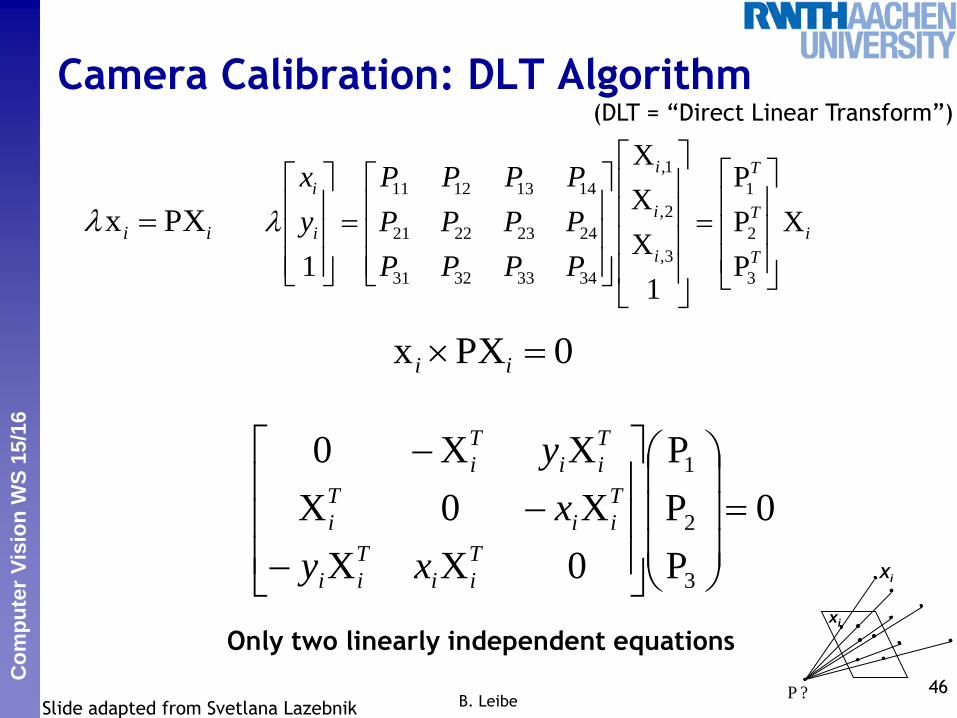
Camera Calibration: DLT Algorithm
46B. Leibe
? P
Xi
xi
Slide adapted from Svetlana Lazebnik
ii PXx
0PXx ii
0
P
P
P
0XX
X0X
XX0
3
2
1
T
ii
T
ii
T
ii
T
i
T
ii
T
i
xy
x
y
Only two linearly independent equations
,1
11 12 13 14 1
,2
21 22 23 24 2
,3
31 32 33 34 3
XP
XP X
X1 P
1
i T
i
i T
i i
i T
x P P P P
y P P P P
P P P P
(DLT = “Direct Linear Transform”)
Perc
eptu
al
and S
enso
ry A
ugm
ente
d C
om
puti
ng
Co
mp
ute
r V
isio
n W
S 1
5/1
6
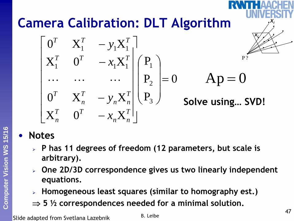
Camera Calibration: DLT Algorithm
• Notes
P has 11 degrees of freedom (12 parameters, but scale is
arbitrary).
One 2D/3D correspondence gives us two linearly independent
equations.
Homogeneous least squares (similar to homography est.)
5 ½ correspondences needed for a minimal solution.47
B. LeibeSlide adapted from Svetlana Lazebnik
0pA 0
P
P
P
X0X
XX0
X0X
XX0
3
2
1111
111
T
nn
TT
n
T
nn
T
n
T
TTT
TTT
x
y
x
y
? P
Xi
xi
Solve using… ?Solve using… SVD!
Perc
eptu
al
and S
enso
ry A
ugm
ente
d C
om
puti
ng
Co
mp
ute
r V
isio
n W
S 1
5/1
6
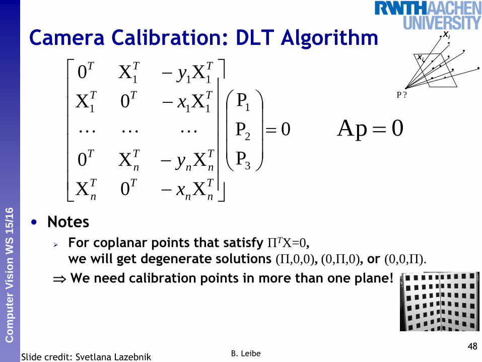
Camera Calibration: DLT Algorithm
• Notes
For coplanar points that satisfy ΠTX=0,
we will get degenerate solutions (Π,0,0), (0,Π,0), or (0,0,Π).
We need calibration points in more than one plane!
48B. LeibeSlide credit: Svetlana Lazebnik
0pA 0
P
P
P
X0X
XX0
X0X
XX0
3
2
1111
111
T
nn
TT
n
T
nn
T
n
T
TTT
TTT
x
y
x
y
? P
Xi
xi

Perc
eptu
al
and S
enso
ry A
ugm
ente
d C
om
puti
ng
Co
mp
ute
r V
isio
n W
S 1
5/1
6
Camera Calibration
• Once we’ve recovered the numerical form of the camera
matrix, we still have to figure out the intrinsic and
extrinsic parameters
• This is a matrix decomposition problem, not an
estimation problem (see F&P sec. 3.2, 3.3)
49B. LeibeSlide credit: Svetlana Lazebnik

Perc
eptu
al
and S
enso
ry A
ugm
ente
d C
om
puti
ng
Co
mp
ute
r V
isio
n W
S 1
5/1
6
Camera Calibration: Some Practical Tips
• For numerical reasons, it is important to carry out some
data normalization.
Translate the image points xi to the (image) origin and scale
them such that their RMS distance to the origin is .
Translate the 3D points Xi to the (world) origin and scale them
such that their RMS distance to the origin is .
(This is valid for compact point distributions on calibration
objects).
• The DLT algorithm presented here is easy to implement,
but there are some more accurate algorithms available
(see H&Z sec. 7.2).
• For practical applications, it is also often needed to
correct for radial distortion. Algorithms for this can be
found in H&Z sec. 7.4, or F&P sec. 3.3. 50B. Leibe
2
3

Perc
eptu
al
and S
enso
ry A
ugm
ente
d C
om
puti
ng
Co
mp
ute
r V
isio
n W
S 1
5/1
6
Topics of This Lecture
• Camera Calibration Camera parameters
Calibration procedure
• Revisiting Epipolar Geometry Triangulation
Calibrated case: Essential matrix
Uncalibrated case: Fundamental matrix
Weak calibration
Epipolar Transfer
• Active Stereo Laser scanning
Kinect sensor
51B. Leibe
Perc
eptu
al
and S
enso
ry A
ugm
ente
d C
om
puti
ng
Co
mp
ute
r V
isio
n W
S 1
5/1
6
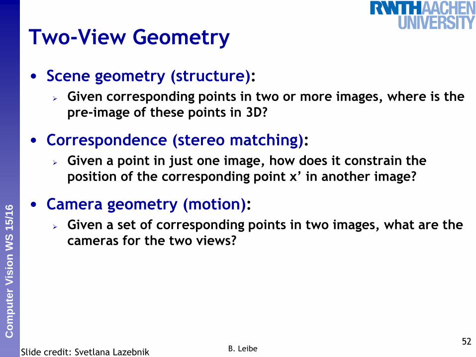
Two-View Geometry
• Scene geometry (structure):
Given corresponding points in two or more images, where is the
pre-image of these points in 3D?
• Correspondence (stereo matching):
Given a point in just one image, how does it constrain the
position of the corresponding point x’ in another image?
• Camera geometry (motion):
Given a set of corresponding points in two images, what are the
cameras for the two views?
52B. LeibeSlide credit: Svetlana Lazebnik
Perc
eptu
al
and S
enso
ry A
ugm
ente
d C
om
puti
ng
Co
mp
ute
r V
isio
n W
S 1
5/1
6
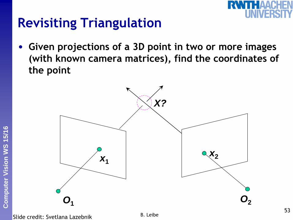
Revisiting Triangulation
• Given projections of a 3D point in two or more images
(with known camera matrices), find the coordinates of
the point
53B. Leibe
O1O2
x1x2
X?
Slide credit: Svetlana Lazebnik

Perc
eptu
al
and S
enso
ry A
ugm
ente
d C
om
puti
ng
Co
mp
ute
r V
isio
n W
S 1
5/1
6
Revisiting Triangulation
• We want to intersect the two visual rays corresponding
to x1 and x2, but because of noise and numerical errors,
they will never meet exactly. How can this be done?
54B. Leibe
O1O2
x1x2
X?
Slide credit: Svetlana Lazebnik
R1R2
Perc
eptu
al
and S
enso
ry A
ugm
ente
d C
om
puti
ng
Co
mp
ute
r V
isio
n W
S 1
5/1
6
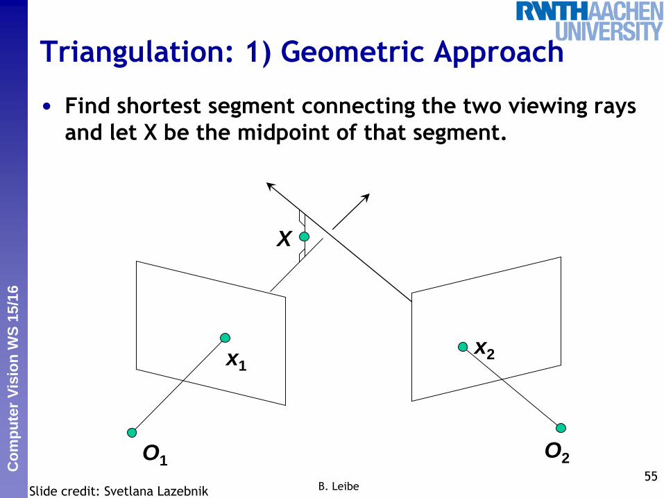
Triangulation: 1) Geometric Approach
• Find shortest segment connecting the two viewing rays
and let X be the midpoint of that segment.
55B. Leibe
O1O2
x1x2
X
Slide credit: Svetlana Lazebnik
Perc
eptu
al
and S
enso
ry A
ugm
ente
d C
om
puti
ng
Co
mp
ute
r V
isio
n W
S 1
5/1
6
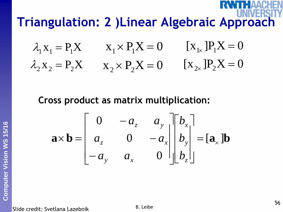
Triangulation: 2 )Linear Algebraic Approach
56B. Leibe
baba ][
0
0
0
z
y
x
xy
xz
yz
b
b
b
aa
aa
aa
XPx
XPx
222
111
0XPx
0XPx
22
11
0XP][x
0XP][x
22
11
Cross product as matrix multiplication:
Slide credit: Svetlana Lazebnik
Perc
eptu
al
and S
enso
ry A
ugm
ente
d C
om
puti
ng
Co
mp
ute
r V
isio
n W
S 1
5/1
6
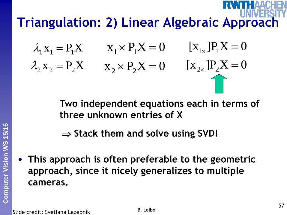
• This approach is often preferable to the geometric
approach, since it nicely generalizes to multiple
cameras.
Triangulation: 2) Linear Algebraic Approach
57B. Leibe
XPx
XPx
222
111
0XPx
0XPx
22
11
0XP][x
0XP][x
22
11
Slide credit: Svetlana Lazebnik
Two independent equations each in terms of
three unknown entries of X
Stack them and solve using… ? Stack them and solve using SVD!
Perc
eptu
al
and S
enso
ry A
ugm
ente
d C
om
puti
ng
Co
mp
ute
r V
isio
n W
S 1
5/1
6
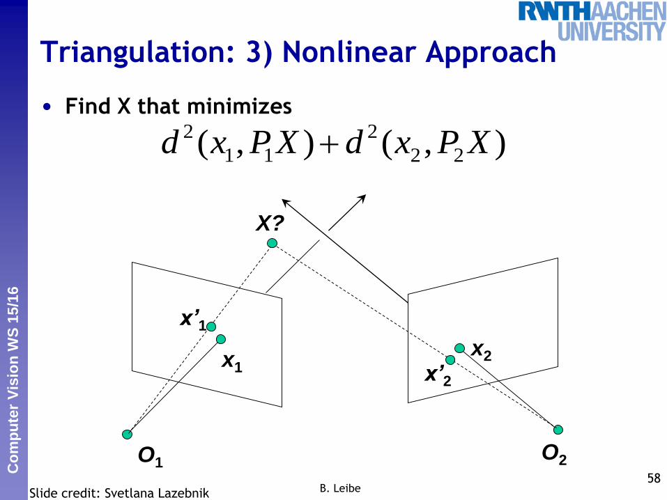
Triangulation: 3) Nonlinear Approach
• Find X that minimizes
58B. Leibe
),(),( 22
2
11
2 XPxdXPxd
O1O2
x1x2
X?
x’1
x’2
Slide credit: Svetlana Lazebnik

Perc
eptu
al
and S
enso
ry A
ugm
ente
d C
om
puti
ng
Co
mp
ute
r V
isio
n W
S 1
5/1
6
Triangulation: 3) Nonlinear Approach
• Find X that minimizes
• This approach is the most accurate, but unlike the other
two methods, it doesn’t have a closed-form solution.
• Iterative algorithm
Initialize with linear estimate.
Optimize with Gauss-Newton or Levenberg-Marquardt
(see F&P sec. 3.1.2 or H&Z Appendix 6).
59B. Leibe
),(),( 22
2
11
2 XPxdXPxd
Perc
eptu
al
and S
enso
ry A
ugm
ente
d C
om
puti
ng
Co
mp
ute
r V
isio
n W
S 1
5/1
6
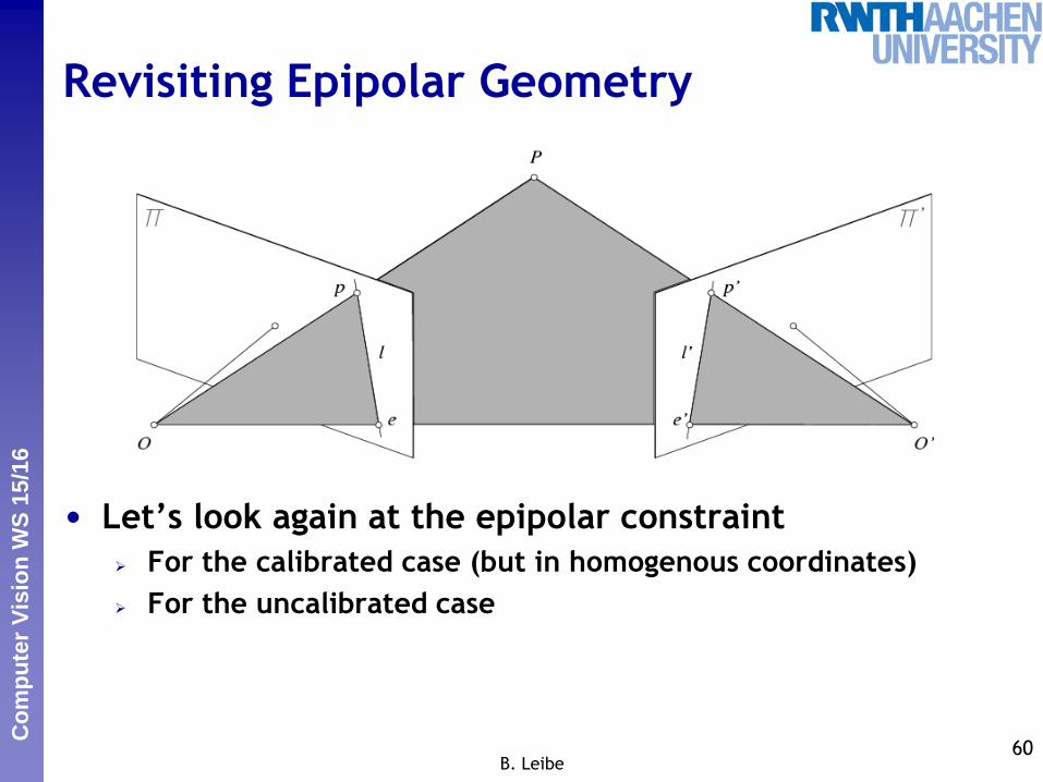
Revisiting Epipolar Geometry
• Let’s look again at the epipolar constraint
For the calibrated case (but in homogenous coordinates)
For the uncalibrated case
60B. Leibe

Perc
eptu
al
and S
enso
ry A
ugm
ente
d C
om
puti
ng
Co
mp
ute
r V
isio
n W
S 1
5/1
6
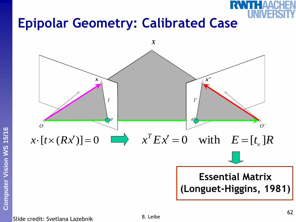
Epipolar Geometry: Calibrated Case
61B. Leibe
X
x x’
Camera matrix: [I|0]X = (u, v, w, 1)T
x = (u, v, w)T
Camera matrix: [RT | –RTt]Vector x’ in second coord.
system has coordinates Rx’ in
the first one.
t
The vectors x, t, and Rx’ are coplanar
R
Slide credit: Svetlana Lazebnik
Perc
eptu
al
and S
enso
ry A
ugm
ente
d C
om
puti
ng
Co
mp
ute
r V
isio
n W
S 1
5/1
6
Epipolar Geometry: Calibrated Case
62B. Leibe
X
x x’
Slide credit: Svetlana Lazebnik
Essential Matrix
(Longuet-Higgins, 1981)
0)]([ xRtx RtExExT ][with0

Perc
eptu
al
and S
enso
ry A
ugm
ente
d C
om
puti
ng
Co
mp
ute
r V
isio
n W
S 1
5/1
6
Epipolar Geometry: Calibrated Case
• E x’ is the epipolar line associated with x’ (l = E x’)
• ETx is the epipolar line associated with x (l’ = ETx)
• E e’ = 0 and ETe = 0
• E is singular (rank two)
• E has five degrees of freedom (up to scale)63
B. Leibe
X
x x’
Slide credit: Svetlana Lazebnik
0)]([ xRtx RtExExT ][with0
Perc
eptu
al
and S
enso
ry A
ugm
ente
d C
om
puti
ng
Co
mp
ute
r V
isio
n W
S 1
5/1
6
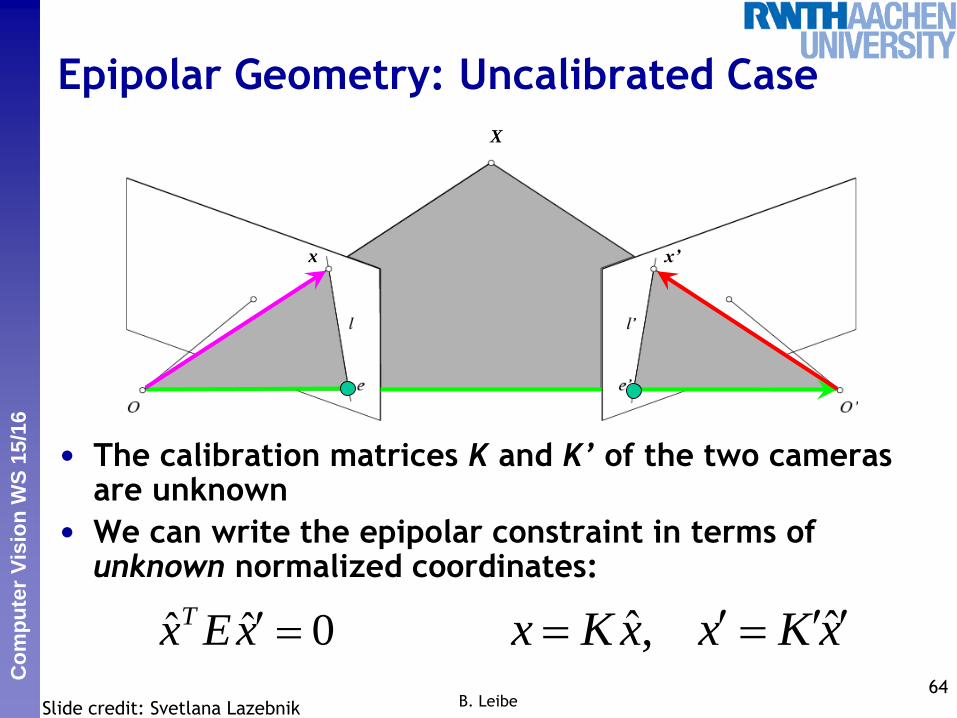
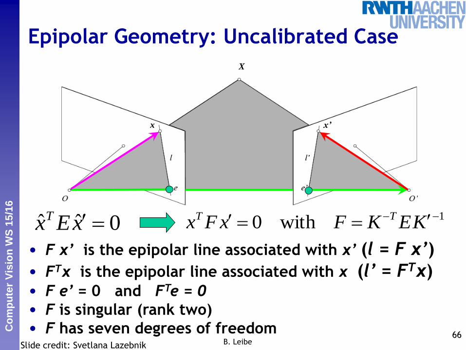
Epipolar Geometry: Uncalibrated Case
• The calibration matrices K and K’ of the two cameras are unknown
• We can write the epipolar constraint in terms of unknown normalized coordinates:
64B. Leibe
X
x x’
Slide credit: Svetlana Lazebnik
0ˆˆ xExT xKxxKx ˆ,ˆ
Perc
eptu
al
and S
enso
ry A
ugm
ente
d C
om
puti
ng
Co
mp
ute
r V
isio
n W
S 1
5/1
6
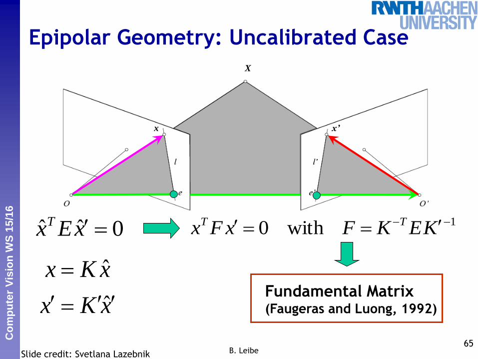
Epipolar Geometry: Uncalibrated Case
65B. Leibe
X
x x’
Slide credit: Svetlana Lazebnik
Fundamental Matrix(Faugeras and Luong, 1992)
0ˆˆ xExT
xKx
xKx
ˆ
ˆ
1with0 KEKFxFx TT
Perc
eptu
al
and S
enso
ry A
ugm
ente
d C
om
puti
ng
Co
mp
ute
r V
isio
n W
S 1
5/1
6
Epipolar Geometry: Uncalibrated Case
• F x’ is the epipolar line associated with x’ (l = F x’)
• FTx is the epipolar line associated with x (l’ = FTx)• F e’ = 0 and FTe = 0
• F is singular (rank two)
• F has seven degrees of freedom66
B. Leibe
X
x x’
Slide credit: Svetlana Lazebnik
0ˆˆ xExT 1with0 KEKFxFx TT

Perc
eptu
al
and S
enso
ry A
ugm
ente
d C
om
puti
ng
Co
mp
ute
r V
isio
n W
S 1
5/1
6
• The Fundamental matrix defines the epipolar geometry
between two uncalibrated cameras.
• How can we estimate F from an image pair?
We need correspondences…
Estimating the Fundamental Matrix
67B. Leibe
xi
Xi
x0i
P? P0?
Perc
eptu
al
and S
enso
ry A
ugm
ente
d C
om
puti
ng
Co
mp
ute
r V
isio
n W
S 1
5/1
6
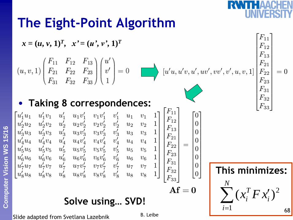
The Eight-Point Algorithm
68B. Leibe
x = (u, v, 1)T, x’ = (u’, v’, 1)T
This minimizes:
2
1
)( i
N
i
T
i xFx
Slide adapted from Svetlana Lazebnik
[u0u; u0v; u0; uv0; vv0; v0; u; v; 1]
26666666666664
F11
F12
F13
F21
F22
F23
F31
F32
F33
37777777777775
= 0
266666666664
u01u1 u0
1v1 u01 u1v
01 v1v
01 v0
1 u1 v1 1
u02u2 u0
2v2 u02 u2v
02 v2v
02 v0
2 u2 v2 1
u03u3 u0
3v3 u03 u3v
03 v3v
03 v0
3 u3 v3 1
u04u4 u0
4v4 u04 u4v
04 v4v
04 v0
4 u4 v4 1
u05u5 u0
5v5 u05 u5v
05 v5v
05 v0
5 u5 v5 1
u06u6 u0
6v6 u06 u6v
06 v6v
06 v0
6 u6 v6 1
u07u7 u0
7v7 u07 u7v
07 v7v
07 v0
7 u7 v7 1
u08u8 u0
8v8 u08 u8v
08 v8v
08 v0
8 u8 v8 1
377777777775
26666666666664
F11
F12
F13
F21
F22
F23
F31
F32
F33
37777777777775
=
266666666664
0
0
0
0
0
0
0
0
377777777775
Af = 0
Solve using… ?Solve using… SVD!
• Taking 8 correspondences:

Perc
eptu
al
and S
enso
ry A
ugm
ente
d C
om
puti
ng
Co
mp
ute
r V
isio
n W
S 1
5/1
6
Excursion: Properties of SVD
• Frobenius norm
Generalization of the Euclidean norm to matrices
• Partial reconstruction property of SVD
Let i i=1,…,N be the singular values of A.
Let Ap = UpDpVpT be the reconstruction of A when we set
p+1,…, N to zero.
Then Ap = UpDpVpT is the best rank-p approximation of A in the
sense of the Frobenius norm
(i.e. the best least-squares approximation).69
2
1 1
m n
ijFi j
A a
min( , )
2
1
m n
i
i
B. Leibe
Perc
eptu
al
and S
enso
ry A
ugm
ente
d C
om
puti
ng
Co
mp
ute
r V
isio
n W
S 1
5/1
6
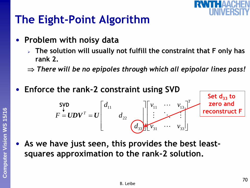
The Eight-Point Algorithm
• Problem with noisy data
The solution will usually not fulfill the constraint that F only has
rank 2.
There will be no epipoles through which all epipolar lines pass!
• Enforce the rank-2 constraint using SVD
• As we have just seen, this provides the best least-
squares approximation to the rank-2 solution.
70B. Leibe
11 11 13
22
33 31 33
T
T
d v v
F d
d v v
UDV U
SVD
Set d33 to
zero and
reconstruct F
Perc
eptu
al
and S
enso
ry A
ugm
ente
d C
om
puti
ng
Co
mp
ute
r V
isio
n W
S 1
5/1
6
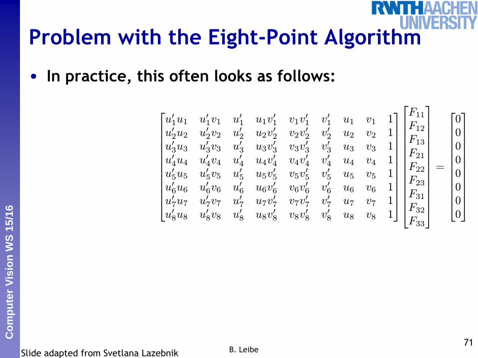
Problem with the Eight-Point Algorithm
71B. Leibe
266666666664
u01u1 u0
1v1 u01 u1v
01 v1v
01 v0
1 u1 v1 1
u02u2 u0
2v2 u02 u2v
02 v2v
02 v0
2 u2 v2 1
u03u3 u0
3v3 u03 u3v
03 v3v
03 v0
3 u3 v3 1
u04u4 u0
4v4 u04 u4v
04 v4v
04 v0
4 u4 v4 1
u05u5 u0
5v5 u05 u5v
05 v5v
05 v0
5 u5 v5 1
u06u6 u0
6v6 u06 u6v
06 v6v
06 v0
6 u6 v6 1
u07u7 u0
7v7 u07 u7v
07 v7v
07 v0
7 u7 v7 1
u08u8 u0
8v8 u08 u8v
08 v8v
08 v0
8 u8 v8 1
377777777775
26666666666664
F11
F12
F13
F21
F22
F23
F31
F32
F33
37777777777775
=
266666666664
0
0
0
0
0
0
0
0
377777777775
Slide adapted from Svetlana Lazebnik
• In practice, this often looks as follows:

Perc
eptu
al
and S
enso
ry A
ugm
ente
d C
om
puti
ng
Co
mp
ute
r V
isio
n W
S 1
5/1
6
Problem with the Eight-Point Algorithm
• In practice, this often looks as follows:
Poor numerical conditioning
Can be fixed by rescaling the data
72B. Leibe
266666666664
u01u1 u0
1v1 u01 u1v
01 v1v
01 v0
1 u1 v1 1
u02u2 u0
2v2 u02 u2v
02 v2v
02 v0
2 u2 v2 1
u03u3 u0
3v3 u03 u3v
03 v3v
03 v0
3 u3 v3 1
u04u4 u0
4v4 u04 u4v
04 v4v
04 v0
4 u4 v4 1
u05u5 u0
5v5 u05 u5v
05 v5v
05 v0
5 u5 v5 1
u06u6 u0
6v6 u06 u6v
06 v6v
06 v0
6 u6 v6 1
u07u7 u0
7v7 u07 u7v
07 v7v
07 v0
7 u7 v7 1
u08u8 u0
8v8 u08 u8v
08 v8v
08 v0
8 u8 v8 1
377777777775
26666666666664
F11
F12
F13
F21
F22
F23
F31
F32
F33
37777777777775
=
266666666664
0
0
0
0
0
0
0
0
377777777775
Slide adapted from Svetlana Lazebnik

Perc
eptu
al
and S
enso
ry A
ugm
ente
d C
om
puti
ng
Co
mp
ute
r V
isio
n W
S 1
5/1
6
The Normalized Eight-Point Algorithm
1. Center the image data at the origin, and scale it so the
mean squared distance between the origin and the data
points is 2 pixels.
2. Use the eight-point algorithm to compute F from the
normalized points.
3. Enforce the rank-2 constraint using SVD.
4. Transform fundamental matrix back to original units: if
T and T’ are the normalizing transformations in the two
images, than the fundamental matrix in original
coordinates is TT F T’.73
B. Leibe [Hartley, 1995]Slide credit: Svetlana Lazebnik
11 11 13
22
33 31 33
T
T
d v v
F d
d v v
UDV U
SVD
Set d33 to
zero and
reconstruct F
Perc
eptu
al
and S
enso
ry A
ugm
ente
d C
om
puti
ng
Co
mp
ute
r V
isio
n W
S 1
5/1
6
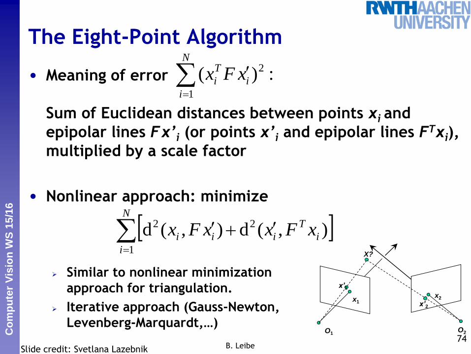
The Eight-Point Algorithm
• Meaning of error
Sum of Euclidean distances between points xi and
epipolar lines Fx’i (or points x’i and epipolar lines FTxi),
multiplied by a scale factor
• Nonlinear approach: minimize
Similar to nonlinear minimization
approach for triangulation.
Iterative approach (Gauss-Newton,
Levenberg-Marquardt,…)74
B. Leibe
:)( 2
1
i
N
i
T
i xFx
N
i
i
T
iii xFxxFx1
22 ),(d),(d
O1O2
x1x2
X?
x’1
x’2
Slide credit: Svetlana Lazebnik
Perc
eptu
al
and S
enso
ry A
ugm
ente
d C
om
puti
ng
Co
mp
ute
r V
isio
n W
S 1
5/1
6
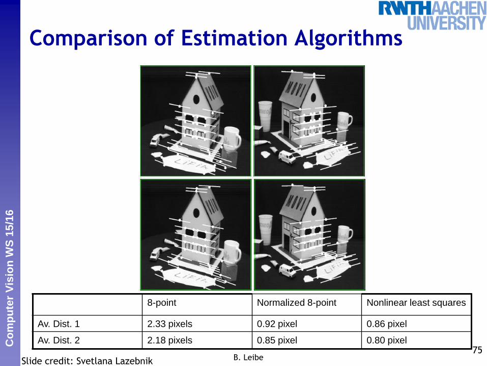
Comparison of Estimation Algorithms
75B. Leibe
8-point Normalized 8-point Nonlinear least squares
Av. Dist. 1 2.33 pixels 0.92 pixel 0.86 pixel
Av. Dist. 2 2.18 pixels 0.85 pixel 0.80 pixel
Slide credit: Svetlana Lazebnik
Perc
eptu
al
and S
enso
ry A
ugm
ente
d C
om
puti
ng
Co
mp
ute
r V
isio
n W
S 1
5/1
6
3D Reconstruction with Weak Calibration
• Want to estimate world geometry without requiring calibrated cameras.
• Many applications: Archival videos
Photos from multiple unrelated users
Dynamic camera system
• Main idea:
Estimate epipolar geometry from a (redundant) set of point correspondences between two uncalibrated cameras.
76B. LeibeSlide credit: Kristen Grauman
Perc
eptu
al
and S
enso
ry A
ugm
ente
d C
om
puti
ng
Co
mp
ute
r V
isio
n W
S 1
5/1
6
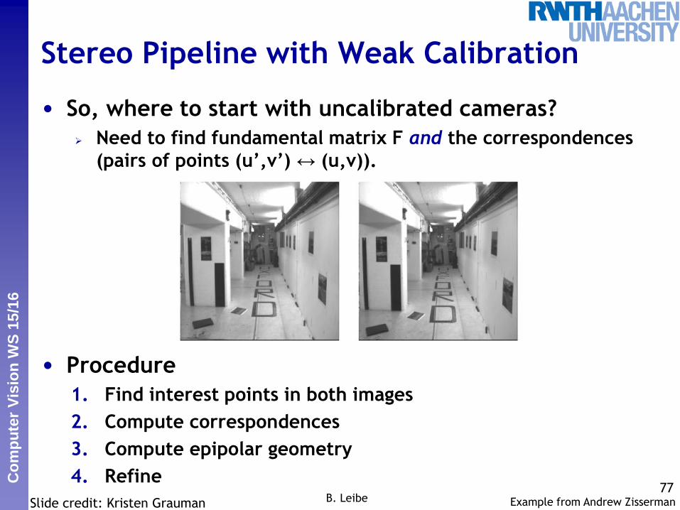
Stereo Pipeline with Weak Calibration
• So, where to start with uncalibrated cameras?
Need to find fundamental matrix F and the correspondences
(pairs of points (u’,v’) ↔ (u,v)).
• Procedure
1. Find interest points in both images
2. Compute correspondences
3. Compute epipolar geometry
4. Refine77
B. Leibe Example from Andrew ZissermanSlide credit: Kristen Grauman

Perc
eptu
al
and S
enso
ry A
ugm
ente
d C
om
puti
ng
Co
mp
ute
r V
isio
n W
S 1
5/1
6
Stereo Pipeline with Weak Calibration
1. Find interest points (e.g. Harris corners)
78B. Leibe Example from Andrew ZissermanSlide credit: Kristen Grauman

Perc
eptu
al
and S
enso
ry A
ugm
ente
d C
om
puti
ng
Co
mp
ute
r V
isio
n W
S 1
5/1
6
Stereo Pipeline with Weak Calibration
2. Match points using only proximity
79B. Leibe Example from Andrew ZissermanSlide credit: Kristen Grauman

Perc
eptu
al
and S
enso
ry A
ugm
ente
d C
om
puti
ng
Co
mp
ute
r V
isio
n W
S 1
5/1
6
Putative Matches based on Correlation Search
80B. Leibe Example from Andrew Zisserman
Perc
eptu
al
and S
enso
ry A
ugm
ente
d C
om
puti
ng
Co
mp
ute
r V
isio
n W
S 1
5/1
6
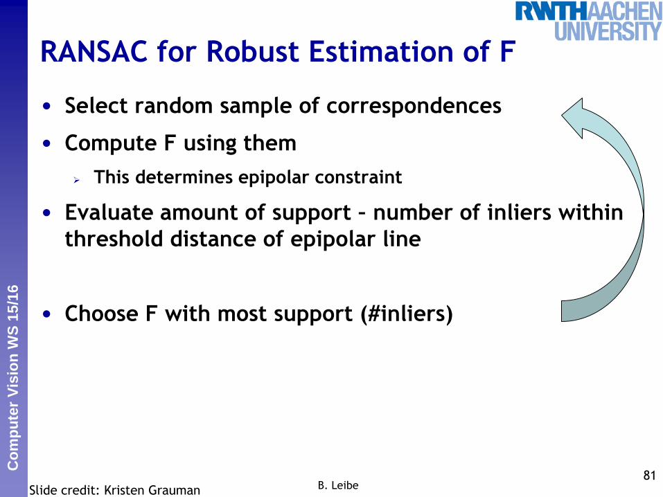
RANSAC for Robust Estimation of F
• Select random sample of correspondences
• Compute F using them
This determines epipolar constraint
• Evaluate amount of support – number of inliers within
threshold distance of epipolar line
• Choose F with most support (#inliers)
81B. LeibeSlide credit: Kristen Grauman

Perc
eptu
al
and S
enso
ry A
ugm
ente
d C
om
puti
ng
Co
mp
ute
r V
isio
n W
S 1
5/1
6
Putative Matches based on Correlation Search
82B. Leibe Example from Andrew Zisserman
Perc
eptu
al
and S
enso
ry A
ugm
ente
d C
om
puti
ng
Co
mp
ute
r V
isio
n W
S 1
5/1
6
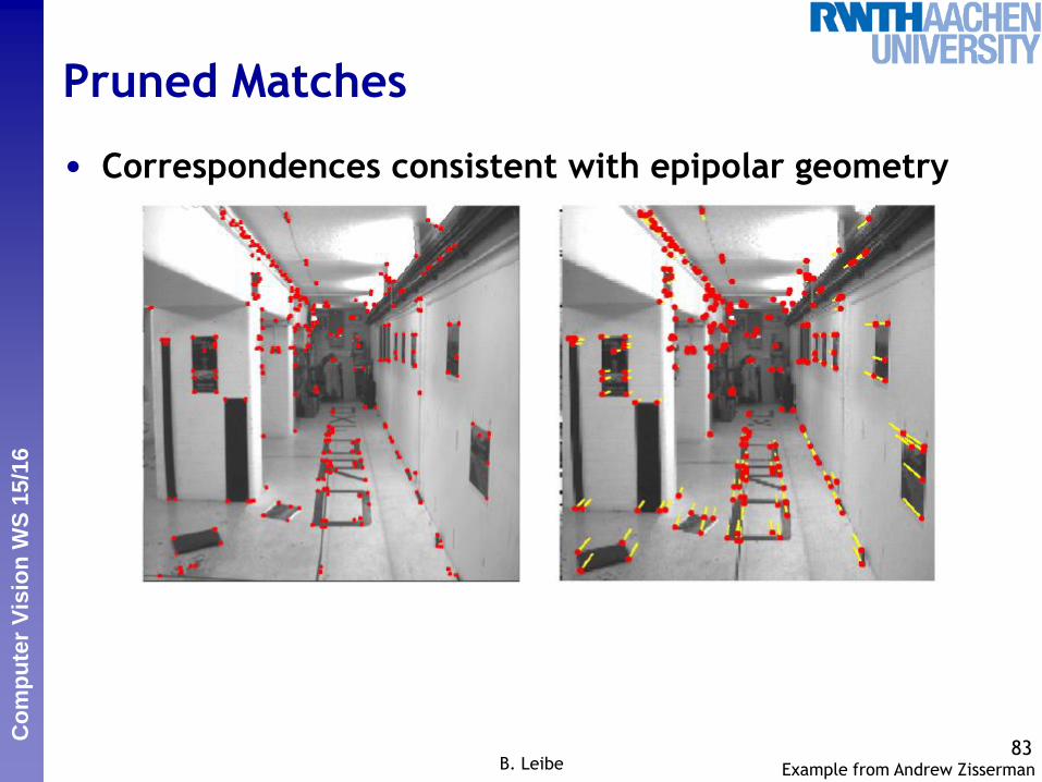
Pruned Matches
• Correspondences consistent with epipolar geometry
83B. Leibe Example from Andrew Zisserman

Perc
eptu
al
and S
enso
ry A
ugm
ente
d C
om
puti
ng
Co
mp
ute
r V
isio
n W
S 1
5/1
6
Resulting Epipolar Geometry
84B. Leibe Example from Andrew Zisserman
Perc
eptu
al
and S
enso
ry A
ugm
ente
d C
om
puti
ng
Co
mp
ute
r V
isio
n W
S 1
5/1
6
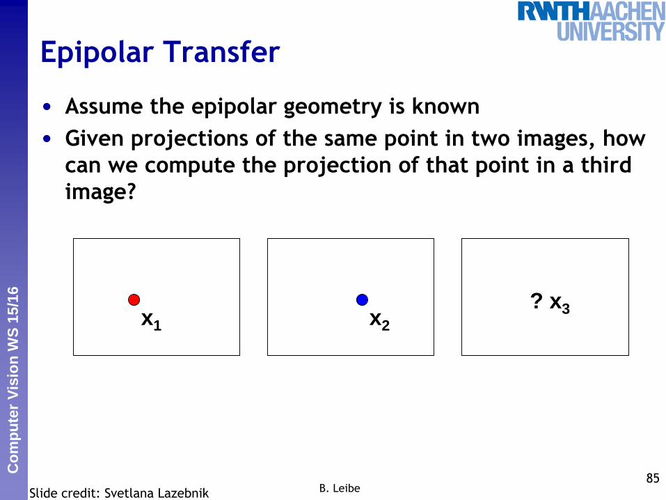
Epipolar Transfer
• Assume the epipolar geometry is known
• Given projections of the same point in two images, how
can we compute the projection of that point in a third
image?
85B. Leibe
x1 x2
? x3
Slide credit: Svetlana Lazebnik
Perc
eptu
al
and S
enso
ry A
ugm
ente
d C
om
puti
ng
Co
mp
ute
r V
isio
n W
S 1
5/1
6
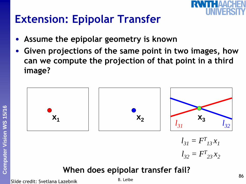
Extension: Epipolar Transfer
• Assume the epipolar geometry is known
• Given projections of the same point in two images, how
can we compute the projection of that point in a third
image?
86B. Leibe
x1 x2 x3l32l31
l31 = FT13 x1
l32 = FT23 x2
When does epipolar transfer fail?
Slide credit: Svetlana Lazebnik
Perc
eptu
al
and S
enso
ry A
ugm
ente
d C
om
puti
ng
Co
mp
ute
r V
isio
n W
S 1
5/1
6
Topics of This Lecture
• Camera Calibration Camera parameters
Calibration procedure
• Revisiting Epipolar Geometry Triangulation
Calibrated case: Essential matrix
Uncalibrated case: Fundamental matrix
Weak calibration
Epipolar Transfer
• Active Stereo Laser scanning
Kinect sensor
87B. Leibe

Perc
eptu
al
and S
enso
ry A
ugm
ente
d C
om
puti
ng
Co
mp
ute
r V
isio
n W
S 1
5/1
6
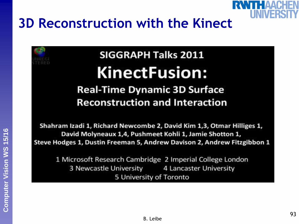
Microsoft Kinect – How Does It Work?
• Built-in IR
projector
• IR camera for
depth
• Regular camera
for color
88B. Leibe
Perc
eptu
al
and S
enso
ry A
ugm
ente
d C
om
puti
ng
Co
mp
ute
r V
isio
n W
S 1
5/1
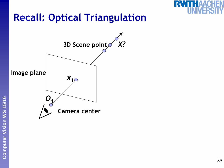
6
Recall: Optical Triangulation
89
O1
x1
X?
Image plane
Camera center
3D Scene point
Perc
eptu
al
and S
enso
ry A
ugm
ente
d C
om
puti
ng
Co
mp
ute
r V
isio
n W
S 1
5/1
6
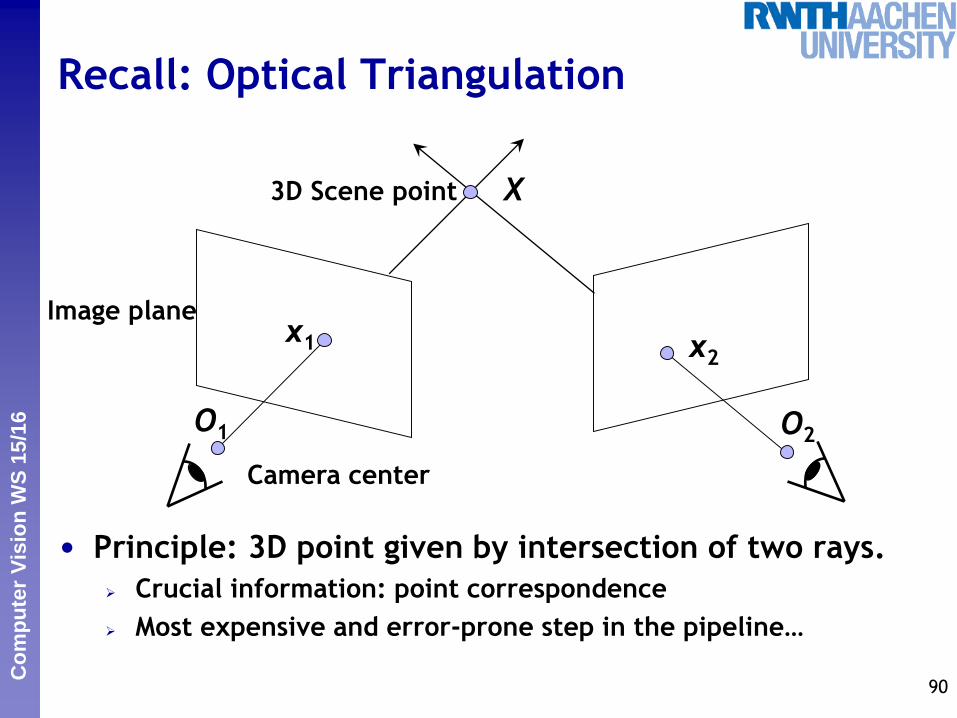
Recall: Optical Triangulation
• Principle: 3D point given by intersection of two rays.
Crucial information: point correspondence
Most expensive and error-prone step in the pipeline…
90
O1 O2
x1 x2
X
Image plane
Camera center
3D Scene point
Perc
eptu
al
and S
enso
ry A
ugm
ente
d C
om
puti
ng
Co
mp
ute
r V
isio
n W
S 1
5/1
6
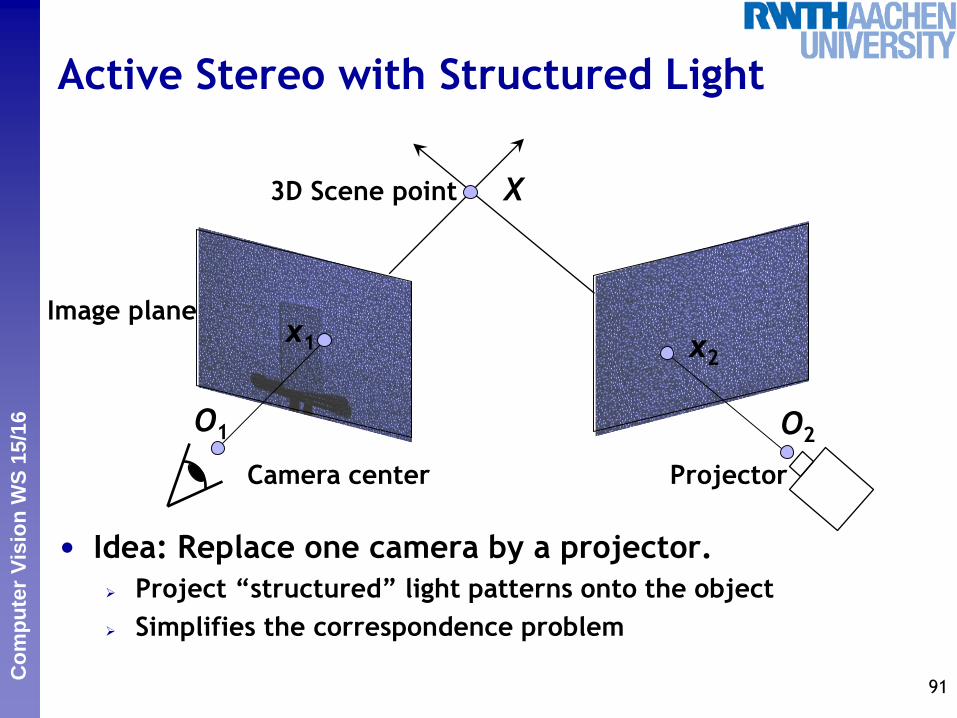
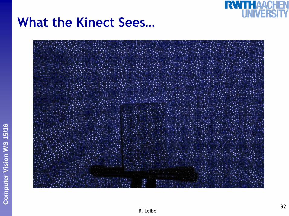
Active Stereo with Structured Light
• Idea: Replace one camera by a projector.
Project “structured” light patterns onto the object
Simplifies the correspondence problem
91
O1 O2
x1 x2
X
Image plane
Camera center
3D Scene point
Projector
Perc
eptu
al
and S
enso
ry A
ugm
ente
d C
om
puti
ng
Co
mp
ute
r V
isio
n W
S 1
5/1
6
What the Kinect Sees…
92B. Leibe
Perc
eptu
al
and S
enso
ry A
ugm
ente
d C
om
puti
ng
Co
mp
ute
r V
isio
n W
S 1
5/1
6
3D Reconstruction with the Kinect
93B. Leibe

Perc
eptu
al
and S
enso
ry A
ugm
ente
d C
om
puti
ng
Co
mp
ute
r V
isio
n W
S 1
5/1
6
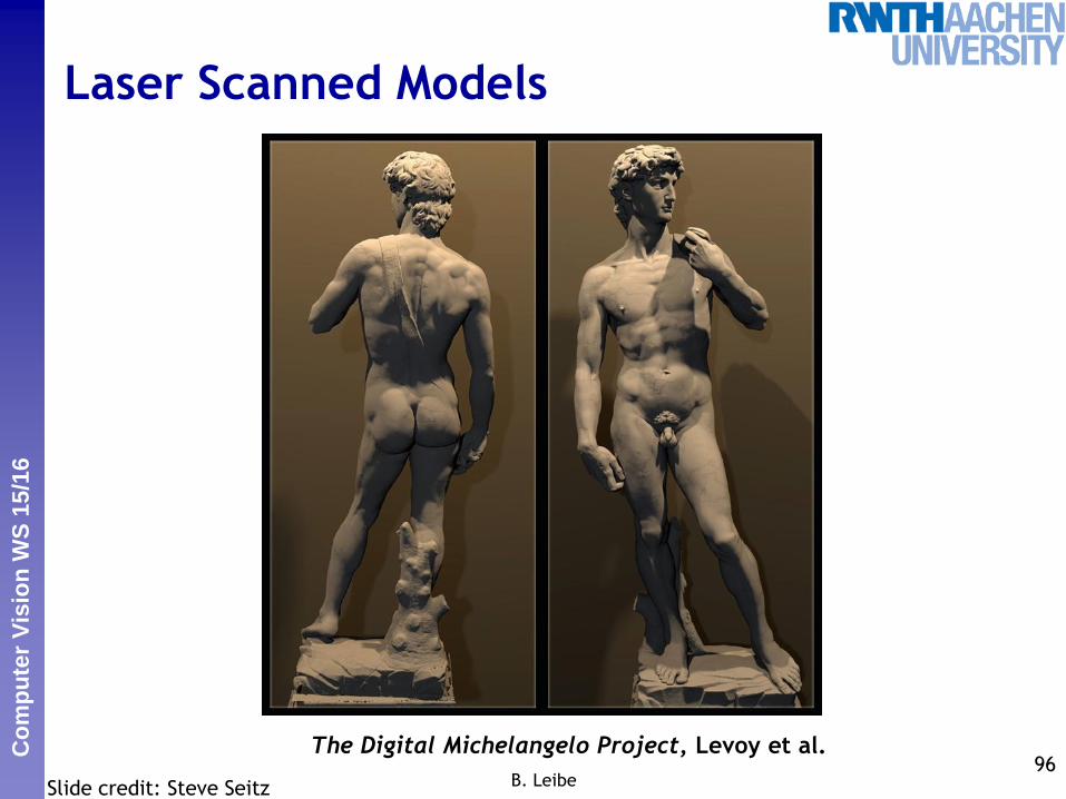
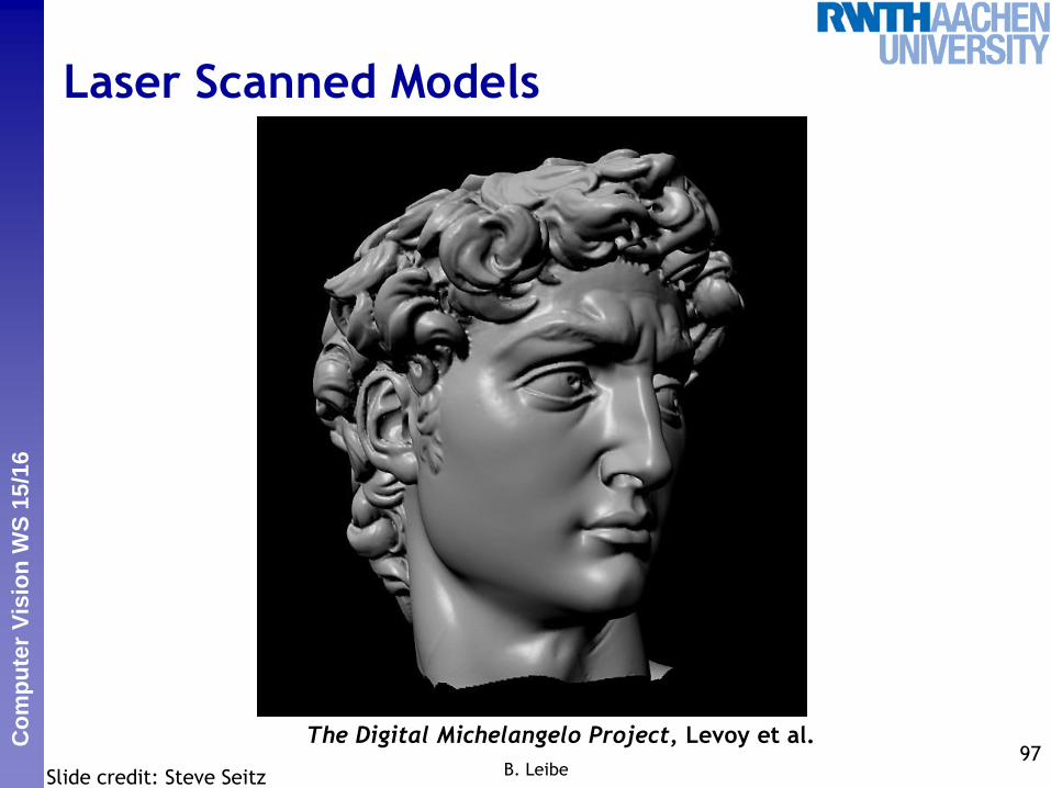
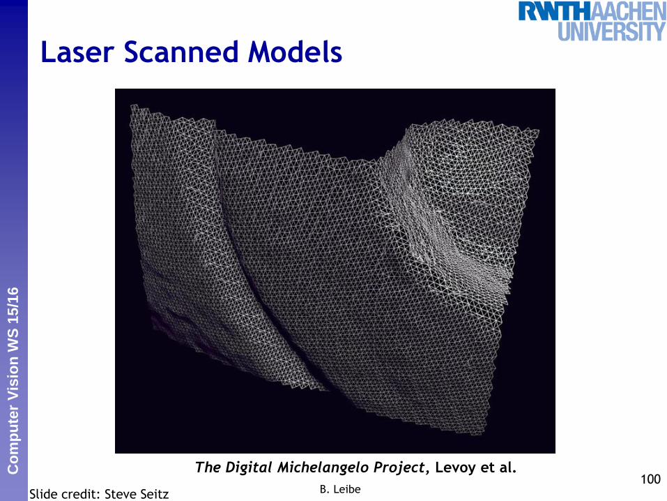
Laser Scanning
• Optical triangulation
Project a single stripe of laser light
Scan it across the surface of the object
This is a very precise version of structured light scanning
95B. Leibe
Digital Michelangelo Projecthttp://graphics.stanford.edu/projects/mich/
Slide credit: Steve Seitz
Perc
eptu
al
and S
enso
ry A
ugm
ente
d C
om
puti
ng
Co
mp
ute
r V
isio
n W
S 1
5/1
6
Laser Scanned Models
96B. Leibe
The Digital Michelangelo Project, Levoy et al.
Slide credit: Steve Seitz
Perc
eptu
al
and S
enso
ry A
ugm
ente
d C
om
puti
ng
Co
mp
ute
r V
isio
n W
S 1
5/1
6
Laser Scanned Models
97B. Leibe
The Digital Michelangelo Project, Levoy et al.
Slide credit: Steve Seitz

Perc
eptu
al
and S
enso
ry A
ugm
ente
d C
om
puti
ng
Co
mp
ute
r V
isio
n W
S 1
5/1
6
Laser Scanned Models
98B. Leibe
The Digital Michelangelo Project, Levoy et al.
Slide credit: Steve Seitz

Perc
eptu
al
and S
enso
ry A
ugm
ente
d C
om
puti
ng
Co
mp
ute
r V
isio
n W
S 1
5/1
6
Laser Scanned Models
99B. Leibe
The Digital Michelangelo Project, Levoy et al.
Slide credit: Steve Seitz
Perc
eptu
al
and S
enso
ry A
ugm
ente
d C
om
puti
ng
Co
mp
ute
r V
isio
n W
S 1
5/1
6
Laser Scanned Models
100B. Leibe
The Digital Michelangelo Project, Levoy et al.
Slide credit: Steve Seitz

Perc
eptu
al
and S
enso
ry A
ugm
ente
d C
om
puti
ng
Co
mp
ute
r V
isio
n W
S 1
5/1
6
Poor Man’s Scanner
107Bouget and Perona, ICCV’98

Perc
eptu
al
and S
enso
ry A
ugm
ente
d C
om
puti
ng
Co
mp
ute
r V
isio
n W
S 1
5/1
6
Slightly More Elaborate (But Still Cheap)
108B. Leibe
http://www.david-laserscanner.com/
Software freely available from Robotics Institute TU Braunschweig
Perc
eptu
al
and S
enso
ry A
ugm
ente
d C
om
puti
ng
Co
mp
ute
r V
isio
n W
S 1
5/1
6
References and Further Reading
• Background information on camera models and
calibration algorithms can be found in Chapters 6 and 7
of
• Also recommended: Chapter 9 of the same book on
Epipolar geometry and the Fundamental Matrix and
Chapter 11.1-11.6 on automatic computation of F.
B. Leibe109
R. Hartley, A. Zisserman
Multiple View Geometry in Computer Vision
2nd Ed., Cambridge Univ. Press, 2004