computer vision - inside minesinside.mines.edu/.../eeng512/lectures/14-siftbasedobjectrecog.pdf ·...
TRANSCRIPT

Computer Vision Colorado School of Mines
Colorado School of Mines
Computer Vision
Professor William Hoff
Dept of Electrical Engineering &Computer Science
http://inside.mines.edu/~whoff/ 1

Computer Vision Colorado School of Mines
SIFT-Based Object Recognition
2

Computer Vision Colorado School of Mines
SIFT-Based Object Recognition
• SIFT – “Scale-invariant feature transform”
• Training phase – We have one or more training images of an object
– We extract SIFT features from the images and put them into a database
• Testing phase – We extract SIFT features from a test image
– We match them to the features in the database
– We find a subset of matches that may be mutually consistent with one of the training images
– We calculate a transformation from the training image to the test image … if all matches are consistent, we have found the object
3
Lowe, D. G., “Distinctive Image Features from Scale-Invariant Keypoints”, Int’l Journal of Computer Vision, 60, 2, pp. 91-110, 2004.

Computer Vision Colorado School of Mines
SIFT – Scale Invariant Feature Transform
• Approach:
– Create a scale space of images • Construct a set of progressively Gaussian blurred images
• Take differences to get a “difference of Gaussian” pyramid (similar to a Laplacian of Gaussian)
– Find local extrema in this scale-space. Choose keypoints from the extrema
– For each keypoint, in a 16x16 window, find histograms of gradient directions
– Create a feature vector out of these
4

Computer Vision Colorado School of Mines
SIFT Software
• Matlab code – http://www.vlfeat.org – Download and put in a directory (such as
C:\Users\whoff\Documents\Research\SIFT\vlfeat-0.9.18) – At the Matlab prompt, run(‘C:\Users\whoff\Documents\Research\SIFT\vlfeat-0.9.18\toolbox\vl_setup’);
• Main functions – vl_sift – extract SIFT features from an image – vl_ubcmatch – match two sets of SIFT features
• Also useful – vl_plotframe – overlay SIFT feature locations on an image – vl_plotsiftdescriptor – overlay SIFT feature details on an
image
5

Computer Vision Colorado School of Mines
Example Images
6
Original source of images: http://www.computing.dundee.ac.uk/staff/jessehoey/teaching/vision/project1.html
Note – in practical applications you would want multiple training images of each object, from different viewpoints
A “test” image
Trai
nin
g im
ages

Computer Vision Colorado School of Mines
Extract SIFT features
• Function call
[f,d] = vl_sift (I)
• Returns
– Arrays f(4,N), d(128,N), where N is the number of features
– f(1:4,i) is (x,y,scale,angle) for the ith feature
– d(1:128,i) is the 128-element descriptor for the ith feature
7
I1 = imread('images/book1.pgm');
I1 = single(I1); % Convert to single precision floating point
if size(I1,3)>1 I1 = rgb2gray(I1); end
imshow(I1,[]);
% These parameters limit the number of features detected
peak_thresh = 0; % increase to limit; default is 0
edge_thresh = 10; % decrease to limit; default is 10
[f1,d1] = vl_sift(I1, ...
'PeakThresh', peak_thresh, ...
'edgethresh', edge_thresh );
fprintf('Number of frames (features) detected: %d\n', size(f1,2));
% Show all SIFT features detected
h = vl_plotframe(f1) ;
set(h,'color','y','linewidth',2) ;

Computer Vision Colorado School of Mines
8
Number of frames (features) detected: 1815
Computer Vision Colorado School of Mines
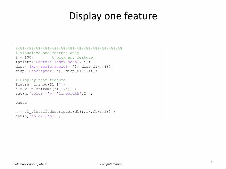
Display one feature
9
%%%%%%%%%%%%%%%%%%%%%%%%%%%%%%%%%%%%%%%%%%%%%%%
% Visualize one feature only
i = 100; % pick any feature
fprintf('Feature index %d\n', i);
disp('(x,y,scale,angle): '); disp(f1(:,i));
disp('Descriptor: '); disp(d1(:,i));
% Display that feature
figure, imshow(I1,[]);
h = vl_plotframe(f1(:,i)) ;
set(h,'color','y','linewidth',2) ;
pause
h = vl_plotsiftdescriptor(d1(:,i),f1(:,i)) ;
set(h,'color','g') ;

Computer Vision Colorado School of Mines
10
Feature index 100 (x,y,scale,angle): 44.9308 393.9326 2.1388 -4.3216

Computer Vision Colorado School of Mines
11
Descriptor: 66 40 13 6 4 4 8 32 19 8 2 28 110 61 4 12 23 50 69 37 58 28 3 7 :

Computer Vision Colorado School of Mines
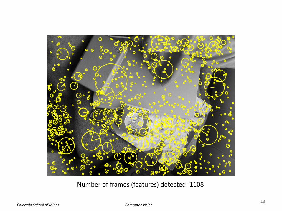
Extract SIFT features – 2nd image
12
%%%%%%%%%%%%%%%%%%%%%%%%%%%%%%%%%%%%%%
% Second image
I2 = single( imread('images/Img01.pgm') );
if size(I2,3)>1 I2 = rgb2gray(I2); end figure, imshow(I2,[]);
% These parameters limit the number of features detected
peak_thresh = 0; % increase to limit; default is 0
edge_thresh = 10; % decrease to limit; default is 10
[f2,d2] = vl_sift(I2, ...
'PeakThresh', peak_thresh, ...
'edgethresh', edge_thresh );
fprintf('Number of frames (features) detected: %d\n', size(f2,2));
% Show all SIFT features detected
h = vl_plotframe(f2) ;
set(h,'color','y','linewidth',2) ;
Computer Vision Colorado School of Mines
13
Number of frames (features) detected: 1108

Computer Vision Colorado School of Mines
Match SIFT features
• Function call
[matches, scores] = vl_ubcmatch(d1, d2);
• Returns
– Arrays: matches(2,M), scores(M), where M is the number of matches
– matches(1:2,i) are the indices of the features for the ith match
– scores(i) is the squared Euclidean distance between the features
14
%%%%%%%%%%%%%%%%%%%%%%%%%%%%%%%%%
% Threshold for matching
% Descriptor D1 is matched to a descriptor D2 only if the distance d(D1,D2)
% multiplied by THRESH is not greater than the distance of D1 to all other
% descriptors
thresh = 2.0; % default = 1.5; increase to limit matches
[matches, scores] = vl_ubcmatch(d1, d2, thresh);
fprintf('Number of matching frames (features): %d\n', size(matches,2));
indices1 = matches(1,:); % Get matching features
f1match = f1(:,indices1);
d1match = d1(:,indices1);
indices2 = matches(2,:);
f2match = f2(:,indices2);
d2match = d2(:,indices2);

Computer Vision Colorado School of Mines
Display matches
• These are potential matches, based on similarity of local appearance
• Many may be incorrect
• There is no notion (yet) of mutual consistency
15
%%%%%%%%%%%%%%%%%%%%%%%%%%%%%%%%%%%%%%%%%%%%%%%%%%%%%%%%
% Show matches
figure, imshow([I1,I2],[]);
o = size(I1,2) ;
line([f1match(1,:);f2match(1,:)+o], ...
[f1match(2,:);f2match(2,:)]) ;
for i=1:size(f1match,2)
x = f1match(1,i);
y = f1match(2,i);
text(x,y,sprintf('%d',i), 'Color', 'r');
end
for i=1:size(f2match,2)
x = f2match(1,i);
y = f2match(2,i);
text(x+o,y,sprintf('%d',i), 'Color', 'r');
end

Computer Vision Colorado School of Mines
16
Number of matching frames (features): 25
12
3
4
5
67 8
9
10
11
12
13
14
15
16
17
18
19
20
21
22
23
24
25
1
23
4
5
67
8
9
10
1112
13
14
1516
17
18
19
20
2122
23
2425

Computer Vision Colorado School of Mines
Consistency
• We want to find a consistent subset of matches – It is consistent if we can derive a rigid transformation that aligns
the two sets of features, with low error residual
• How to find this subset? – We could use RANSAC – But RANSAC doesn’t work well if we have a lot of outliers
• Instead we will use clustering (Hough transform) – Potential matches vote for poses in the space of all possible
poses – The pose with the highest number of votes is probably correct – We can use those matches to calculate a more accurate
transformation
17

Computer Vision Colorado School of Mines
Transformation
• Ideally, we would calculate the essential matrix (or fundamental) matrix that aligns the two sets of points – Then we could calculate a 6 DOF pose transformation – However, this is expensive
• Hough space is 6 dimensional • We need 8 points to calculate the essential matrix1
• Instead, Lowe uses a simplified transformation – A 2D scaled rotation, from training image to test image – Cheap to compute
• Hough space is 4-dimensional (x,y,scale,angle) • A single feature match can vote for a transformation
– It’s only an approximation, valid for • Planar patches • Small out-of-plane rotation • Scale changes and in-plane rotation ok
– So use a coarse Hough space • Main purpose is to identify valid matches • Then calculate a more refined transformation later
18
1Although 8 points is needed for the linear algorithm, as few as 5 points can be used in a nonlinear algorithm

Computer Vision Colorado School of Mines
Pose Clustering
• The feature in the training image is located at (x1,y1) – So the “origin” of the object in the training image
is located at a vector offset of v1 = (-x1,-y1) with respect to this feature
• If we find a matching feature in the test image at (x2,y2) – We can apply the same offset to its location, to
determine where the origin of the object is in this image
– However, we need to scale and rotate v1, using the relative scale and angle of the feature
• Consistent matches should vote for – The same relative scale and angle – The same location of the object origin in the test
image
19
v1
v1
v2
(x1,y1)
(x2,y2)
(x2,y2)

Computer Vision Colorado School of Mines
Scale and Rotation
• Given – (x1,y1,a1,s1) from image 1
– (x2,y2,a2,s2) from image 2
• Let – v1 = (-x1,-y1)T
– sr = s1/s2 % scale ratio
– da = a1 – a2 % difference in angles (-p..p)
• Then – v2 = R*(v1/sr)
– where R is the rotation matrix
20
)cos()sin(
)sin()cos(
dada
dadaR
v2
(x2,y2)
v1
(x1,y1)

Computer Vision Colorado School of Mines
21
%%%%%%%%%%%%%%%%%%%%%%%%%%%%%%%%%%%%%%%%%%%%%%%%%%%%%%%
% Between all pairs of matching features, compute
% orientation difference, scale ratio, and center offset
allScales = zeros(1,size(matches,2)); % Store computed values
allAngs = zeros(1,size(matches,2));
allX = zeros(1,size(matches,2));
allY = zeros(1,size(matches,2));
for i=1:size(matches, 2)
fprintf('Match %d: image 1 (scale,orient = %f,%f) matches', ...
i, f1match(3,i), f1match(4,i));
fprintf(' image 2 (scale,orient = %f,%f)\n', ...
f2match(3,i), f2match(4,i));
scaleRatio = f1match(3,i)/f2match(3,i);
dTheta = f1match(4,i) - f2match(4,i);
% Force dTheta to be between -pi and +pi
while dTheta > pi dTheta = dTheta - 2*pi; end
while dTheta < -pi dTheta = dTheta + 2*pi; end
allScales(i) = scaleRatio;
allAngs(i) = dTheta;
x1 = f1match(1,i); % the feature in image 1
y1 = f1match(2,i);
x2 = f2match(1,i); % the feature in image 2
y2 = f2match(2,i);
% The "center" of the object in image 1 is located at an offset of
% (-x1,-y1) relative to the detected feature. We need to scale and rotate
% this offset and apply it to the image 2 location.
offset = [-x1; -y1];
offset = offset / scaleRatio; % Scale to match image 2 scale
offset = [cos(dTheta) +sin(dTheta); -sin(dTheta) cos(dTheta)]*offset;
allX(i) = x2 + offset(1);
allY(i) = y2 + offset(2);
end
figure, plot(allScales, allAngs, '.'), xlabel('scale'), ylabel('angle');
figure, plot(allX, allY, '.'), xlabel('x'), ylabel('y');
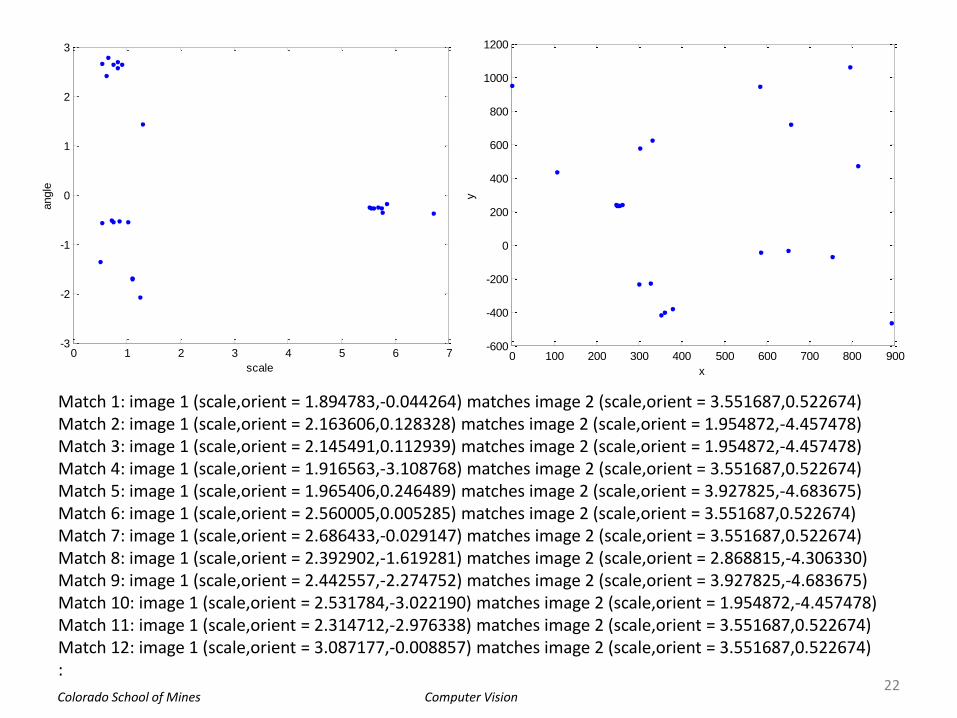
Computer Vision Colorado School of Mines
22
0 1 2 3 4 5 6 7-3
-2
-1
0
1
2
3
scale
angle
0 100 200 300 400 500 600 700 800 900-600
-400
-200
0
200
400
600
800
1000
1200
x
y
Match 1: image 1 (scale,orient = 1.894783,-0.044264) matches image 2 (scale,orient = 3.551687,0.522674) Match 2: image 1 (scale,orient = 2.163606,0.128328) matches image 2 (scale,orient = 1.954872,-4.457478) Match 3: image 1 (scale,orient = 2.145491,0.112939) matches image 2 (scale,orient = 1.954872,-4.457478) Match 4: image 1 (scale,orient = 1.916563,-3.108768) matches image 2 (scale,orient = 3.551687,0.522674) Match 5: image 1 (scale,orient = 1.965406,0.246489) matches image 2 (scale,orient = 3.927825,-4.683675) Match 6: image 1 (scale,orient = 2.560005,0.005285) matches image 2 (scale,orient = 3.551687,0.522674) Match 7: image 1 (scale,orient = 2.686433,-0.029147) matches image 2 (scale,orient = 3.551687,0.522674) Match 8: image 1 (scale,orient = 2.392902,-1.619281) matches image 2 (scale,orient = 2.868815,-4.306330) Match 9: image 1 (scale,orient = 2.442557,-2.274752) matches image 2 (scale,orient = 3.927825,-4.683675) Match 10: image 1 (scale,orient = 2.531784,-3.022190) matches image 2 (scale,orient = 1.954872,-4.457478) Match 11: image 1 (scale,orient = 2.314712,-2.976338) matches image 2 (scale,orient = 3.551687,0.522674) Match 12: image 1 (scale,orient = 3.087177,-0.008857) matches image 2 (scale,orient = 3.551687,0.522674) :

Computer Vision Colorado School of Mines
Hough Transform
• Use a 4-D pose space
– Dimensions are (angle,scale,x,y)
– Have coarse bins
• Angles are –p..p, by increments of p/4
• Scales are 0.5 .. 10 by increments of 2.0
• x is 1..N by increments of W/5
• y is 1..N by increments of H/5
23
• Use coarse bins because
– Fast
– Transformation is only approximate anyway
• Note
– Lowe recommends also voting for neighboring bins
– Mitigates problem with boundary effects

Computer Vision Colorado School of Mines
24
% Use a coarse Hough space.
% Dimensions are [angle, scale, x, y]
% Define bin centers
aBin = -pi:(pi/4):pi;
sBin = 0.5:(2):10;
xBin = 1:(size(I2,2)/5):size(I2,2);
yBin = 1:(size(I2,1)/5):size(I2,1);
H = zeros(length(aBin), length(sBin), length(xBin), length(yBin));
for i=1:size(matches, 2)
a = allAngs(i);
s = allScales(i);
x = allX(i);
y = allY(i);
% Find bin that is closest to a,s,x,y
[~, ia] = min(abs(a-aBin));
[~, is] = min(abs(s-sBin));
[~, ix] = min(abs(x-xBin));
[~, iy] = min(abs(y-yBin));
H(ia,is,ix,iy) = H(ia,is,ix,iy) + 1; % Inc accumulator array
end
% Find all bins with 3 or more features
[ap,sp,xp,yp] = ind2sub(size(H), find(H>=3));
fprintf('Peaks in the Hough array:\n');
for i=1:length(ap)
fprintf('%d: %d points, (a,s,x,y) = %f,%f,%f,%f\n', ...
i, H(ap(i), sp(i), xp(i), yp(i)), ...
aBin(ap(i)), sBin(sp(i)), xBin(xp(i)), yBin(yp(i)) );
end

Computer Vision Colorado School of Mines 25
Peaks in the Hough array: 1: 4 points, (a,s,x,y) = -0.785398,0.500000,385.000000,1.000000 2: 3 points, (a,s,x,y) = -1.570796,0.500000,513.000000,1.000000 3: 7 points, (a,s,x,y) = 0.000000,6.500000,257.000000,193.000000 4: 3 points, (a,s,x,y) = 2.356194,0.500000,513.000000,385.000000
>> size(H) ans = 9 5 5 5
>> H(:,:,3,3) ans = 0 0 0 0 0 0 0 0 0 0 0 0 0 0 0 0 0 0 0 0 0 0 0 7 0 0 0 0 0 0 0 0 0 0 0 0 0 0 0 0 0 0 0 0 0

Computer Vision Colorado School of Mines
• Get features corresponding to largest bin – Of course, if there are multiple instances of the object, you should
look at multiple bins
26
%%%%%%%%%%%%%%%%%%%%%%%%%%%%%%%%%%%%%%%%%%%%%%%%%%%%%%%%%%%%%%
% Get the features corresponding to the largest bin
nFeatures = max(H(:)); % Number of features in largest bin
fprintf('Largest bin contains %d features\n', nFeatures);
[ap,sp,xp,yp] = ind2sub(size(H), find(H == nFeatures));
indices = []; % Make a list of indices
for i=1:size(matches, 2)
a = allAngs(i);
s = allScales(i);
x = allX(i);
y = allY(i);
% Find bin that is closest to a,s,x,y
[~, ia] = min(abs(a-aBin));
[~, is] = min(abs(s-sBin));
[~, ix] = min(abs(x-xBin));
[~, iy] = min(abs(y-yBin));
if ia==ap(1) && is==sp(1) && ix==xp(1) && iy==yp(1)
indices = [indices i];
end
end
fprintf('Features belonging to highest peak:\n');
disp(indices);

Computer Vision Colorado School of Mines
• Display matches corresponding to largest bin
27
% Show matches to features in largest bin as line segments
figure, imshow([I1,I2],[]);
o = size(I1,2) ;
line([f1match(1,indices);f2match(1,indices)+o], ...
[f1match(2,indices);f2match(2,indices)]) ;
for i=1:length(indices)
x = f1match(1,indices(i));
y = f1match(2,indices(i));
text(x,y,sprintf('%d',indices(i)), 'Color', 'r');
end
for i=1:length(indices)
x = f2match(1,indices(i));
y = f2match(2,indices(i));
text(x+o,y,sprintf('%d',indices(i)), 'Color', 'r');
end

Computer Vision Colorado School of Mines
28
19
20
21
22
23
24
25
19
20
2122
23
2425
Largest bin contains 7 features Features belonging to highest peak: 19 20 21 22 23 24 25

Computer Vision Colorado School of Mines
Affine Transform
• Finally, fit a 2D affine transformation to the potential set of correct matches (≥3)
• This will give a better approximation to the true 6 DOF transform, than the initial scaled-rotation transform found by Hough
• Checking residual errors also allows us to make sure matches are correct
• A 2D affine transform is valid for – Planar patches undergoing small out-of-
plane rotation – In-plane rotation and scale changes are ok
29
11 12
21 22
1 0 0 1 1
B x A
B y A
x a a t x
y a a t y
• Notes – You could detect
outliers and throw them out
– If more points are available you might fit an essential matrix

Computer Vision Colorado School of Mines
30
%%%%%%%%%%%%%%%%%%%%%%%%%%%%%%%%%%%%%%%%%%%%%%%%%%%%%%%%%%%%%%
% Fit an affine transformation to those features.
% We use affine transformation because the image of a planar surface
% undergoing a small out-of-plane rotation can be approximated by an
% affine transformation.
% Create lists of corresponding points pA and pB.
pA = [f1match(1,indices); f1match(2,indices)];
pB = [f2match(1,indices); f2match(2,indices)];
N = size(pA,2);
% Calculate the transformation T from I1 to I2; ie p2 = T p1.
A = zeros(2*N,6);
for i=1:N
A( 2*(i-1)+1, :) = [ pA(1,i) pA(2,i) 0 0 1 0];
A( 2*(i-1)+2, :) = [ 0 0 pA(1,i) pA(2,i) 0 1];
end
b = reshape(pB, [], 1);
x = A\b;
T = [ x(1) x(2) x(5);
x(3) x(4) x(6);
0 0 1];
fprintf('Derived affine transformation:\n');
disp(T);
r = A*x-b; % Residual error
ssr = sum(r.^2); % Sum of squared residuals
% Estimate the error for each image point measurement.
% For N image points, we get two measurements from each, so there are 2N
% quantities in the sum. However, we have 6 degrees of freedom in the result.
sigmaImg = sqrt(ssr/(2*N-6)); % Estimated image std deviation
fprintf('#pts = %d, estimated image error = %f pixels\n', N, sigmaImg);

Computer Vision Colorado School of Mines
31
Derived affine transformation: 0.1820 -0.0435 246.0450 0.0462 0.1701 235.7885 0 0 1.0000 #pts = 7, estimated image error = 0.295452 pixels
>> A A = 319.2146 73.9901 0 0 1.0000 0 0 0 319.2146 73.9901 0 1.0000 419.3207 406.6396 0 0 1.0000 0 0 0 419.3207 406.6396 0 1.0000 232.7990 113.5247 0 0 1.0000 0 0 0 232.7990 113.5247 0 1.0000 257.8340 79.1712 0 0 1.0000 0 0 0 257.8340 79.1712 0 1.0000 289.6241 211.9763 0 0 1.0000 0 0 0 289.6241 211.9763 0 1.0000 185.0680 37.5656 0 0 1.0000 0 0 0 185.0680 37.5656 0 1.0000 249.7681 138.1065 0 0 1.0000 0 0 0 249.7681 138.1065 0 1.0000
>> x x = 0.1820 -0.0435 0.0462 0.1701 246.0450 235.7885
>> b b = 300.8143 263.1026 304.9128 324.3566 283.6000 265.7888 289.6536 261.2126 288.7967 285.1844 278.1984 250.7712 285.6681 270.8394

Computer Vision Colorado School of Mines
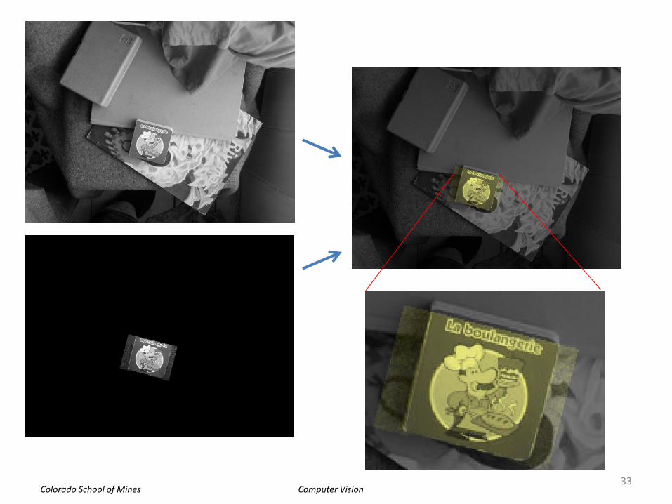
Visualize Match
32
%%%%%%%%%%%%%%%%%%%%%%%%%%%%%%%%%%%%%%%%%%%%%%%%%%%%%%%%%%%%%%
% Ok, apply the transformation to image 1 to align it to image 2.
% We'll use Matlab's imtransform function.
tform = maketform('affine', T');
I3 = imtransform(I1,tform, ...
'XData', [1 size(I1,2)], 'YData', [1 size(I1,1)] );
figure, imshow(I3, []);
% Overlay the images
RGB(:,:,1) = (I2+I3)/2;
RGB(:,:,2) = (I2+I3)/2;
RGB(:,:,3) = I2/2;
RGB = uint8(RGB);
figure, imshow(RGB);
Computer Vision Colorado School of Mines 33

Computer Vision Colorado School of Mines
Some Simplifications
• I only used a single training image of each object; should really have images from multiple viewing angles
• Only looked for a single object from the database
• Only looked for a single instance of the object
• Hough transform: I voted for single bin instead of neighboring bins
• Computed affine transformation only for verification, instead of essential matrix
• I implemented full 4-D Hough array; Lowe uses hash table for speed
34