Computer Vision for Nanoscale Imaging

Eraldo Ribeiro

Department of Computer Sciences

Florida Institute of Technology

Melbourne, FL 32901

Mubarak Shah

Computer Vision Laboratory

School of Computer Science

University of Central Florida

Orlando, FL 32826

Abstract

The main goal of Nanotechnology is to analyze and understand the properties

of matter at the atomic and molecular level. Computer vision is rapidly expanding

into this new and exciting field of application, and considerable research efforts are

currently being spent on developing new image-based characterization techniques to

analyze nanoscale images. Nanoscale characterization requires algorithms to perform

image analysis under extremely challenging conditions such as low signal-to-noise ratio

and low resolution. To achieve this, nanotechnology researchers require imaging tools

that are able to enhance images, detect objects and features, reconstruct 3D geometry,

and tracking. This paper reviews current advances in computer vision and related

areas applied to imaging nanoscale objects. We categorize the algorithms, describe

1

their representative methods, and conclude with several promising directions of future

investigation.

1 Introduction

In this paper, we review the state-of-the-art of computer vision and related areas applied

to imaging applications at the nano scale. Nanotechnology allows us to understand unique

unique properties of matter at atomic and molecular level spanning a wide range of ap-

plications in areas such as medicine, micro-processor manufacturing, material sciences, and

environmental technologies. The use of image-based characterization techniques are essential

to nanoscale research, and the role of image analysis has considerably expanded over the past

few years. Visual inspection of defects, particle selection, and analysis of three-dimensional

structure are few examples of tasks performed with the help of images in nanoscale sciences.

We believe that nanoscale image-based characterization represents a novel and rich field of

application for both computer vision and image processing technologies. Current develop-

ment in computer vision algorithms in object recognition, 3D reconstruction, filtering, and

tracking represent a small sample of the many potential applications of computer vision

research that can be applied to nanoscale imagery.

Traditional computer vision algorithms analyze images generated by the interaction of visible

light with the observed scene. In nanoscale characterization, images are mostly created by

measuring the response of electrons on the material’s surface as they interact with emitted

electron beams and atomic size probes. This non-conventional acquisition process poses

2

several challenges to traditional computer vision methods. Most of these challenges are due

to the type of imaging instrumentation required to analyze objects at such a small scale. In

the following sections, we summarize some of these main challenging factors:

• Extremely low signal-to-noise ratio (SNR). Nanoscale images usually have ex-

tremely low signal to noise ratio even when generated by highly sophisticated imaging

devices such as the Transmission Electron Microscope (TEM) and Scanning Electron

Microscope (SEM). The high level of noise in these images can be considered the major

complicating factor for computer vision algorithms.

• Transparent appearance of specimens. nanoscale objects may have transparent

appearance (e.g., crystals and biological structures). This transparency creates an

extra challenge to algorithms for vision applications such as feature detection, recog-

nition, and 3D reconstruction algorithms.

• Limited number of images per observation. The destructive nature of some

imaging procedures as well as lengthly image acquisition procedures reduce the number

of images that one may use for analysis and training. As a result, computer vision

methods will need to train and work on very reduced data sets that will pose further

challenges to the algorithms.

• Complex image formation geometry. Traditional model (perspective) of imaging

formation does not always constitute a reasonable model for nanoscale imaging devices.

Orthographic and affine projections are usually considered as reasonable approxima-

3

tions of the imaging geometry of electron microscopy. However, more extensive work is

still to be done on modeling the electron image formation process from the computer

vision standpoint.

The amount of research on nanoscale imaging analysis has increased considerably in the

past ten years. Recent advances by both computer vision and image processing communities

combined with the availability of affordable high-performance computer hardware are making

image-based nanoscale characterization an important research field. In this paper, we aim

to provide a review of computer vision and image analysis techniques used for nanoscale

characterization.

A large amount of the current work in the literature deals with the problem of particle detec-

tion. Automatic particle detection is a required step before another main task in nanoscale

imaging, the 3D reconstruction of particles, can be performed. These two tasks are closely

related as the process of reconstructing the 3D geometry of individual particles requires

a large number of images taken from varying angles. In some applications, the required

number of particles to produce reasonable 3D models can be as large as tens of thousands.

Three-dimensional modeling of nanoscale objects is another active area of research. Finally,

image enhancement and virtual reality applications are popular topics.

In this paper, we focus mainly on the application of computer vision to images of objects at

a typical scale of less than 100nm. Images of objects of such a small scale are produced by

electron microscopy such as the scanning electron microscope and the transmission electron

microscope. However, some of the approaches discussed in this paper can also be applied to

4

larger-scale objects. For instance, optical and fluorescence microscopy represent two other

fields with plenty of applications for computer vision algorithms. However, these methods

will not be discussed in this paper, as the resolution of fluorescent microscope is the same as

their optical counterparts. Fluorescent microcopy allows for the characterization of in-vivo

biological specimens that can be processed [77], reconstructed in 3D [69], and tracked [9, 7].

The remainder of this paper is organized as follows. Section 2 reviews the most common

imaging instruments used for characterization of nanoscale objects. Section 3 provides a

taxonomy of the methods. We conclude in Section 4 by summarizing a few directions for

future computer vision research in this new and exciting field of application. As in any new

area of research, there is a large number of problems to be addressed.

2 Nanoscale imaging devices

In this section, we provide a brief description of the most commonly used nanoscale imaging

devices. In order to develop effective image-analysis algorithms it is important to under-

stand the basic principles behind the image formation for each instrument. A more detailed

description of the optics and physical principles used in electron microscopy can be found

in [87, 29, 32]. Nanoscale images are often obtained by measuring the level of energy pro-

duced by the interaction of electrons on the specimen’s surface with a beam of electrons

emitted by the microscope. This is the basic essence of imaging devices such as Scanning

Electron Microscopy (SEM) and Transmission Electron Microscopy (TEM). Images at the

nanoscale are also obtained by measuring the reactive force resulting from the interaction

5

of a nanoscale mechanical stylus-like probe with the specimen’s surface. Atomic Force Mi-

croscopy (AFM) is an example of such a technique. In Figure 1 we illustrate the visualization

range for the currently available major microscopes along with examples of structures that

are visualized at those scales. For comparison purposes, the figure also includes examples of

the resolution range achieved by light microscopy.

0.1 nm 1 nm 10 nm 100 nm 1 µm 10 µm

Electron MicroscopyLight Microscopy

100 µm

Plant and animal cellsBacteriasVirusesProteinMoleculesAtoms

TEM SEMAFM

Figure 1: Visualization scale of nanoscale imaging devices and examples visualized at specific

scales (Adapted from [25]).

In this paper, we focus on images produced by electron microscopy (i.e., TEM[87], AFM

[49] and SEM[87, 29]), as they are the main visualization devices used in current nanotech-

nology characterization. Figure 2 shows examples of images taken using the three types of

microscopes. Below we briefly describe each of them.

Scanning electron microscopy. SEMs construct an image of an object by detecting

electrons resulting from the interaction of a scanning focused-electron beam with the surface

of the object operating in high vacuum. The samples of the analyzed material are required

to be conductive, as insulated samples will produce distorted images. As a result, samples

6

are often coated with a thin layer of metal (e.g., gold coating). The resolution limit depends

mainly on the beam spot size and it can be as small as 1 nm. A common imaging problem

in SEM is the possible reaction of the gas with the beam spot due to possible residuals from

diluted gas that remains in suspension inside the SEM chamber. This reaction considerably

limits the imaging time for true nanoscale objects and often causes a SEM imaging section

to produce only a single noisy image of the observed object. Figure 2(a) shows an example

of a SEM image from a pollen grain. SEM images are 2D dimensional projections of the

3D imaged specimens. The resulting pixel intensity approximately obeys the inverse of

Lambert’s law [52], which states that the flux per unit solid angle leaving a surface in any

direction is proportional to the cosine of the angle between that direction and the normal to

the surface [41].

Transmission Electron Microscopy. TEM can be considered the most powerful and

truly atomic resolution imaging method currently available. It differs from SEM by its so-

phisticated optics and a very small high-energy power beam of electrons that passes through

the sample. Transmittance though samples is required so that the microscope can achieve

visualization at the atomic level. When compared with conventional optical scale images,

transmission microscopy images can have considerably low contrast and extremely low signal-

to-noise ratios (SNR). These are the main problems for surface characterization of true

nanoscale specimens. The imaging process can be time consuming, and tedious manual

tuning results in a limited number of images of each specimen. In Figure 2(b), a carbon

nanotube is imaged using TEM along with a few individual particles.

7

Atomic Force Microscopy. This microscope follows the principle of traditional stylus-

based mechanical profilometers [49]. It uses a sharp-tipped micro cantilever mounted on

a probe tip of the microscope. The probe tip scans the surface of the sample object and

a laser beam measures the probe’s deflections. AFM images are similar to range images

(i.e., surface depth or topography) and resolution is mostly limited by the finite curvature

of the tip. Unfortunately, deflection of the probe tip accounts for the interaction of large

number of atoms, rendering atomic definition unreliable. AFM is capable of better than 1

nm lateral resolution on ideal samples and of 0.01 nm resolution in height measurements.

The 3D surface generated by this microscope does not provide information about the 2D

texture on the analyzed surface as does SEM. An example of a surface obtained using AFM

is shown in Figure 2(c).

(a) (b) (c)

Figure 2: Electron microscope images. (a) SEM image of a pollen grain. (b) TEM image of a

nanotube. (c) AFM image of the surface of living cell (Image from [34]).

Other available methods for nanoscale imaging include Near-Field Scanning Optical Mi-

8

croscopy (NSOM) [68], that uses a sub-wavelength light source as a scanning probe, and the

Superconducting Quantum Interference Device (SQUIDs) that measures magnetic responses

at the nanoscale [30]. New methods for characterization of nanoscale structures are also

being developed [71, 40].

In general, the quality and resolution of images produced by nanoscale characterization

devices depend on various factors, including the nature of the imaged object and the device

characteristics. Table 1 summarizes the information in this section. Low SNR and reduced

number of images are the main limiting factors for the direct application of computer vision

methods to these images. In the next section, we describe current applications of computer

vision methods to nanoscale imagery.

Table 1: Nanoscale Imaging Instruments

Instrument Data Type Typical Resolution Key Points

SEM 2D 3–7nm Non-metalic samples require metalic sputtering.

Inverse Lambertian reflectance.

TEM 2D .10–1nm Demanding sample preparation.

Damaging to biological samples.

Low signal-to-noise-ratio.

AFM 3D 1–100nm Spatial resolution limited by size and shape of probe tip.

9

3 Computer vision methods for nanoscale images

In this section, we categorize and review existing work on nanoscale imaging in the computer

vision literature. Current computer vision methods for nanoscale characterization mostly

deal with four main applications listed below:

1. Image enhancement and noise reduction. Low resolution images with high levels

of noise represent a major problem in nanoscale characterization. Anisotropic diffusion

methods appear to be the most suitable for filtering noisy nanoscale images. These

methods successfully filter noise while preserving relevant edge details in an image.

2. Particle detection. Automatic detection is a required pre-requisite for 3D shape

reconstruction of particles. Accurate modeling requires the identification of thousands

of particles. This application is of primary importance in Structural Biology.

3. Three-dimensional reconstruction. SEM and TEM images are inherently two-

dimensional projections of three-dimensional samples. The reconstruction of the ob-

served object is typically achieved in two main ways: tomographic-like reconstruction

from projections and multiple-view geometry reconstruction based on epipolar geom-

etry constraints.

4. Visualization. Methods for visualization and virtual reality applications at the

nanoscale are strongly related to computer vision techniques such as online tracking,

image fusion, and image-based rendering. Integration of computer vision and virtual

reality can support several aspects of nanoscale characterization.

10

Table 2 summarizes algorithms and lists representative papers on the application of computer

vision techniques these four categories. Next, we provide a general description of these

approaches.

Table 2: Categorization of Computer Vision Methods for Nanoscale Imagery

Approach Representative Work

Image enhancement and noise removal Anisotropic diffusion [76, 8, 77]

Structured illumination for super-resolution [31, 73].

Particle detection Template correlation [63]

Detecting edges [92, 96, 95, 37]

Gray level intensity statistics [79, 91]

Appearance-based recognition [58, 94]

Neural networks [65]

3D reconstruction multiple-view geometry [12, 13, 42]

Tomographic projection reconstruction [43, 85, 74, 81, 60, 28]

Snakes-based stereo reconstruction [44]

Visualization Multi-modal registration for visualization [78, 22, 23]

3.1 Image enhancement and noise removal

One of the major challenges in analyzing images of nanoscale objects is the extremely low

signal-to-noise ratio present in the images even when highly sophisticated imaging devices

11

are used. Addressing this noise problem is a complex task as traditional filtering algorithms

work by attenuating high-frequency content and may cause blurring of relevant details in the

image [10]. Ideally, we would like to preserve relevant image-edge information while removing

undesirable noise. Techniques such as anisotropic diffusion [67, 88] are ideal candidates

to handle this type of problem. Anisotropic diffusion allows for the inclusion of an edge-

stopping function that controls the level of smoothing across relevant image details. The

classic filtering equation as proposed by Perona and Malik [67] can be defined by the following

partial differential equation:

∂I(x, y, t)

∂t= div[g(‖∇I‖)∇I], (1)

where ‖∇I‖ is the gradient magnitude of the image and g(‖∇I‖) is an edge-stopping function

that slows the diffusion across edges. An example of an edge-stopping function is g(x) =

11+x2/K2 for a positive K [67]. In Figure 3, we display results using this method [67] on

two TEM images. The top row shows three noisy images of nanoparticles. The bottom row

shows the filtered versions of each image after performing diffusion-based noise cleaning. The

edges are preserved while the noise content is removed. This is a very important feature for

noise cleaning algorithms in nanoscale imaging as the accuracy of edge location and particles

shapes are essential.

Recently published work demonstrates the potential of these techniques on images of nanoscale

objects [76, 8]. The most representative work on filtering nanoscale images is the work of

Scharr et al. [76, 75], that describes a diffusion-based method for enhancing silicon device

images. Diffusion- based methods are well suited for noise removal in low-quality nanoscale

12

Figure 3: Example of noise removal in TEM images using anisotropic diffusion. Top row:

original noisy images. Bottom row: filtered images.

images. One of the main advantages of this technique is that parameters of robust image

statistics can be learned from examples. Anisotropic diffusion and its relationship to robust

statistics is described in [8].

The method proposed by Scharr et al. [76, 75] works by creating a statistical model of the

noise characteristics and using this model as prior knowledge for reducing noise in low quality

images of silicon devices. The idea is to create prior distribution models for both noise and

13

desired features (edges). The parameters of these distributions are estimated by comparing

image statistics from samples of both low and high quality images of a given imaging device

(e.g., SEM, TEM) and the observed material (e.g., silicon device). Their method is based

on the statistical interpretation of anisotropic diffusion [8], as it allows for a mechanism to

automatically determine what features should be considered as outliers during the filtering

process. Additionally and most importantly, the robust statistics framework allows for the

inclusion of spatial and noise statistics as constraints which can be used to improve continuity

of edges and other important features in the images.

As we mention earlier in this text, the process required to acquire high-quality images of

nanoscale objects can be both time consuming and destructive. As a result, it is usually

preferable to work with lower-quality images. Thus, noise cleaning algorithms are essential

for this type of data. Scharr et al. [75] assumes an additive generative model for the pixels

in the noisy image such that fi = gi + η where fi is the intensity of a pixel in the low-quality

image, gi is the intensity of a pixel in the ground truth image, and η is the noise value

originated from an unknown distribution. It turns out that an empirical estimation of the

distribution can be obtained from the difference between the high- and the low- quality ones.

Figure 4(a) and (b) show an example of a high-quality and a low-quality image of a silicon

circuit board. Figure 4(c) to (d) show the distributions of gray level intensity differences

between two images (a) and (b), and the log distribution of the horizontal edges (a) and

vertical edges (b) respectively.

The next step is to fit known distribution models to the estimated empirical distributions.

14

(a) (b) (c) (d) (e)

(f) (g) (h)

Figure 4: Empirical distributions. (a) High-quality image (ground truth). (b) Low-quality

image. Log distribution of intensity differences (fi − gi). (c) Log distribution of horizontal

edges of the high-quality image. (d) Log distribution of the high-quality image. (All images

from [75])

Scharr et al. [75] use an adapted version of a recently-proposed model for computing the

statistics of images of man-made scenes [53]. Recent work on modeling the statistics of

both natural and man-made images is likely to play an important role on the development

of new methods for enhancing the quality of nanoscale images [39, 53, 33]. Following [53],

Scharr et al. [75] propose the use of t-distribution perturbed by Gaussian noise. The image is

represented by a mixture model [61] in which the first term captures the image edge statistics

15

and the second term captures the image noise:

p(X = x) =w

Z(1 +

x2

σ21

)−t + (1− w)1√

2πσ2

exp(− x2

2σ22

). (2)

In Equation 2, X is a random variable representing an edge filter response for the image (data

difference, horizontal and vertical derivatives), 0 ≤ w ≤ 1 represents the mixture proportions

of the two terms, and Z is a normalization factor that ensures that the integral of the first

term of the equation is 1. Based on the previous assumptions, the image recovering problem

can be cast as the maximum a posteriori estimation problem:

p(g|f) =∏

i

(p(fi|gi)J∏

j=1

p(nj∇gi)), (3)

where p(fi|gi) is defined by the measured image statistics, and p(nj∇gi) is a spatial prior in

terms of local neighborhood derivatives. The maximization of Equation 3 is achieved using

the standard minimization of the negative logarithm. Scharr et al. [75] also propose the use

a B-spline approximation of the likelihood function and apply a gradient descent to estimate

the parameters of that function. The B-spline model is a robust statistics kernel ρ(x) that

allows the problem to be converted to a robust statistics anisotropic diffusion of the following

form:

E(g,∇g) =

∫Ω

ρ0(g(x)− f(x)) + λ

J∑j=1

ρj(|nj∇σg(x)|)dx (4)

where x is a pixel location in the image domain Ω. Figure 4(f)–(h) show some of the

results produced using this method. The above framework can be directly extended to the

multidimensional case. Scharr and Uttenweiller [77] demonstrate the application of the 3D

16

extension of the diffusion filtering to the problem of enhancing time-varying fluorescence

microscopy images of Actin filaments.

The combination of robust statistics and anisotropic diffusion can be considered as one the

most effective methods to enhance the quality of noisy nanoscale images. The framework is

also promising if coupled with other computer vision techniques such as object recognition

and image segmentation. The use of prior knowledge can be extended by employing more

advanced models for spatial interaction [50] rather than simply representing the priors by

means of 1D frequency distributions of edge directions.

3.2 Automatic particle detection

The ability to automatically detect particles in TEM images is essential in cryo-electron

microscopy [62, 94]. Detecting single particles represents the first stage of most 3D single

particle reconstruction algorithms [81, 60, 28]. Usually, a typical particle 3D reconstruction

process would necessarily need to use thousands of or even millions of particles to produce a

reasonable 3D model. This alone makes manual interaction for particle selection unfeasible

and practically impossible. In the literature, the problem of particle selection is by far the

most studied problem in nanoscale computer vision. A recent comparison of particle detec-

tion algorithms for TEM images is presented by [94], and an overview of current methods

can be found in [62].

Methods for particle detection in TEM images can be broadly grouped into two main classes:

non-learning methods and learning methods. Next, we summarize the two approaches.

17

Non-learning methods

The main characteristic of non-learning methods is that they do not require a training or

learning stage. Methods in this group include approaches based on template correlation [63,

4, 80], edge detection [92, 96, 37], and gray level intensity [79, 91]. However, non-learning

methods tend to be less flexible and sensitive to both noise and small variations in particle

appearance when compared to other approaches.

(a)

(a)

(b)

Figure 1. Image pyramids for the (a) template

and (b) mask images, constructed from the

ferritin data set.

(high contrast) and cryo (low contrast) micrographs.

2. A Correlation-Based Particle Picking Algo-

rithm

A real-space correlation-based particle picking algo-

rithm has been developed. This method was chosen since

it can use a normalised correlation function and local

masking[6].

A rotationally averaged particle sum and a binary mask

were constructed, using the IMAGIC software[4]. The

template was constructed by manually selecting a number

of particles, performing translational alignment, averaging,

and then rotationally averaging to obtain a circular, sym-

metric template. The constructed mask is the same size as

the template, and has the value 255 where the template data

is valid, and 0 otherwise.

2.1. Construction of Image Pyramids

The micrographs are sampled finely ( 0.9A per pixel),

consequently the digitised images are generally quite large,

for example, the test dataset images of the protein ferritin

are of size pixels, with a template of size

pixels. The amount of computation can be dra-

matically reduced by performing particle picking using a

lower resolution image, template and mask. Therefore,

image pyramids are constructed, where each level is con-

structed by smoothing the previous level with a Gaussian

filter (to prevent aliasing), and then sub-sampling by a factor

of two. In this manner, the micrograph image dimensions

are progressively halved until one of the image dimensions

is less than 1000 pixels.

(a)

(b)

Figure 2. example of pixel data and shape of

the correlation surface: (a) in the vicinity of a

particle (b) around a spurious maxima, from

the ferritin data set.

Image pyramids are also constructed for the template and

mask images, with the same number of levels as the micro-

graph pyramid. Figure 1 shows the image pyramids for the

template and mask for the ferritin data.

The original full-sized mask is a binary image consisting

only of the values 0 and 255. However, the construction

of the pyramid smooths the pixel values, resulting in pixel

values between 0 and 255, particularly around the edges of

the mask. Therefore, the mask images can be thought of as

weight values, which scale the contribution of each pixel to

the correlation computations.

2.2. Correlation

Computation begins with the lowest resolution (ie,

smallest) image, template and mask. The Normalised Cross

Correlation (NCC) score is computed at each image loca-

tion using Equation (1), resulting in a 2-D array of

scores called a correlation image.

2.3. Selection of Maxima

Locations where the NCC is locally maximal are flagged

as potential particles. At this stage there are often a large

number of maxima which do not correspond to particles.

2.4. Filtering of Maxima

This step determines which of the local maxima corre-

spond to particles, by examining the shape of the correla-

tion surface in the vicinity of each maxima. It was observed

that for particles, the correlation surface consists of a peak

surrounded by a trough, while for spuriousmaxima, the cor-

relation values are more or less flat, as shown in Figure 2.

A recursive region-growing algorithm is used to iden-

tify valid particles. This algorithm starts with local max-

(b) (c) (d)

Figure 5: Detecting particles using correlation-based approach. (a) Original micrograph

image. (b) Template for matching and 3D surface plot of the correlation peak. (c) Correlation

response on entire image. (d) Detected particles (All images from [4]).

Particles in micrograph images tend to have very similar appearance, and sometimes can

be assumed to appear in a reduced number of poses. If the appearance and size of the

particles do not change, template-matching algorithms [14] can help determine the location

of the particles. Template matching based on cross correlation [11] is one of the mostly used

methods for object detection in images. It works by calculating a matching score between

18

a template image and an input image that contains instances of the objects to be detected.

The cross correlation between a template g(x, y) and an image f(x, y) is given by:

f(x, y)⊕ g(x, y) =

∫f(x, y)g(x + α, y + β)dαdβ, (5)

where α and β are dummy variables of integration.

Correlation-based approaches for particle detection work well when the location of the object

is determined mostly by an unknown translation. However, techniques usually generate a

large number of false positives, creating the need for manual intervention. Image noise also

represents a challenge for correlation-based methods and filtering is usually required before

correlation takes place.

Some particle detection uses edge-detection techniques [92, 96, 37]. The process consists of

detecting edges in the micrograph images. The detected edges are grouped into a shape model

used to detect the particles. Examples of such methods include the use of distance transform

and Voronoi diagrams [92], and robust voting-based methods such as Hough transforms [96].

Hough transform-based methods work by accumulating edge angle information in a polar

coordinate system [21]. The peaks of the polar accumulation space represent the coordinates

of the center location of each individual particle. Figure 6 summarizes the process of particle

selection described in [96]. In the Figure, (a) shows the original image where particles are

to be detected, (b) displays the edge map estimated using an edge-detection technique, (c)

shows the Hough accumulation space (highly-voted locations are shown as brighter points),

and (d) shows the final detected particles. The Hough transform allows for the detection of

any generic shapes, circles and rectangles are the simplest ones.

19

(a) (b) (c) (d)

Figure 6: Detecting circular particles using an edge-based Hough transform approach [96].

(a) Original micrograph image. (b) Detected edges. (c) Accumulation space of Hough

transform. (d) Detected particles (All images from [96]).

Analysis of the geometric arrangement of edge information has been used by Yu and Ba-

jaj [92]. The authors describe a particle-detection algorithm that works by fitting Voronoi

diagrams [2] to the distance transform [70, 36] of an edge map. The method allows for the

detection of rectangular and circular particles in micrographs. The strong reliance on edge-

map information makes the method sensitive to noise. To minimize the effects of noise, the

authors suggest the use of filtering techniques such as anisotropic diffusion [67, 88].

Particles in micrographs tend to have an overall dark appearance when compared to the

noisy image brackground. Information on the homogeneity of pixel gray level intensity may

also be used for particle detection. The key idea is to detect individual regions that have

specific concentrations of darker pixels. Yu and Bajaj [91] proposed a gravitation-based

clustering algorithm that is similar to mode-finding algorithms such as the mean shift [17].

The gravitation-based algorithm assumes that particles represent disconnected regions of low

20

pixel intensity. Detection is accomplished by clustering these regions followed by consistency

tests to eliminate false positives connected particles.

Singh et al. proposed a particle detector based on clustering regions containing pixel of low

intensity [79]. In this case, the authors propose the use of a statistical model of pixel-intensity

distribution based on Markov Random Fields [56]. Regions of the micrograph that are likely

to contain particles were determined by a segmentation algorithm and the parameters of the

Markov Random Field were estimated using the Expectation-Maximization algorithm [19].

However, the detection of the correct location of each particle is a slow process and produces

many wrong detections.

The next group of methods use machine-learning techniques to build detectors that are

capable of learning the general appearance of the particles.

Learning-based methods

Learning-based methods typically work in a two-stage process [58, 94]. The first stage is

called learning. During this stage, an appearance model is created from a set of training

images of particles. The learned models will allow for the recognition of particles even under

variations in appearance and a certain level of image noise. The second stage is the detection

stage that consists of scanning the target at every location in the search space for acceptable

matches. The location of the best matches will be the location of the detected particles.

Methods based on neural networks are also included in this group [65].

The image is scanned for the presence of particles that are similar to the learned model.

Methods in this group have the advantage of being both very general (i.e. able to detect

21

particles of any shape) and robust to noise, two critical requirements in TEM image analysis.

As mentioned earlier in this paper, the main problem encountered by current particle detec-

tion algorithms is the inherent SNR in TEM images. As a consequence, boundary and shape

extraction are hard to accomplish. A second problem is that the shape of the particles may

not be geometrically defined, resulting in the need for more complex appearance models.

Learning-based algorithms such as the one proposed by Viola and Jones [86] represent a

promising way to solve the problem of particle detection under noisy conditions. However,

depending on the level of complexity of the objects, the learning stage can be computation-

ally demanding and slow. Additionally, good detection rates depend on the ability of the

classifier to learn a representative model for the particles. This usually requires that a large

numbers of features are measured over a large number of training images.

Mallick et al [58] applies an Adaboost-based learning algorithm to detect particles in Cryo-

EM micrographs. Their method works as follows. First, a training set containing images of

particles and non-particles is used to train the classifier. This is an off-line process. Once

the classifier is trained, an on-line detection process is performed to detect the location of

the particles in the micrograph. Figure 7(a) and (b) show examples of images from both

particle and non-particle training set respectively. Figure 7(c) shows the type of features used

by the classifier during the training stage. Figure 7(d) shows the best-performing features

determined by the Adaboost learning. Figure 7(e)–(g) show a micrograph image and the

resulting detected particles (circular and rectangular, respectively).

The detection stage in [58] uses a two-stage cascade classifier. The cascade design aims at

22

(a) (b) (c) (d)

(e) (f) (g)

Figure 7: Detecting particles using learned features. (a) Images of particles. (b) Images of

non-particles. (c) Multi-scale, multi-orientation rectangular set of features used for training.

(d) Best selected features for detection. (e) Image containing particles to be detected. (f)

Detected rectangular particles. (g) Detected circular particles. (All images from [58]).

speeding the detection process by ruling out most of the non-particle images at the first stage.

The second stage makes the final decision if a subregion should be accepted as a particle.

The key idea here is that a strong classifier can be built from a linear combination of weak

classifiers [86]. In turn, classifier F (t) at each stage is composed of a linear combination of

K simple classifiers based on a single feature (weak classifiers). For example, let fk(t) with

k ∈ 1, . . . , K represent weak classifiers that produce a response +1 or −1 for each particle

23

or non-particle subimages respectively. A strong classifier for a stage of the cascade can be

formed as a linear combination of the weak classifiers as follows:

F (t) =

+1,

∑Kk=1 αkfk(t) ≥ T

∑Kk=1 αk

−1, otherwise.

(6)

where α = (α1, . . . , αK) is a vector of weights indicating the contribution of each classifier to

the final decision and T is a threshold that determines the tradeoff between false-negative

and false-positive rates. The approach consists of training a large number of classifiers fk(t)

using the training sets for particle and non-particle images, and automatically selecting the

best candidates of measurements using the Adaboost algorithm. This algorithm selects and

combines the best set of simple classifiers fk(t) to form a strong classifier that achieves

close to ideal classification rates. The algorithm uses rectangular features, as they are both

fast to compute, and approximate first and second derivatives of the image at a particular

scale. It is worth noting that the weak classifiers can be of any form and are usually simple

univariate threshold-based functions. The strength of this approach lies in the correct choices

of parameters to form the linear combination of weak classifiers achieved via the Adaboost

algorithm.

Improvements to this method can be achieved by pre-filtering the images before training

and detection. However, in principle the algorithm should work for very noisy conditions as

long as the classifier is trained under those same conditions. Additionally, three-dimensional

objects under arbitrary poses can represent a problem to this method. Next, we discuss the

reconstruction of 3D models of nanoscale structures.

24

3.3 3D reconstruction of nano-objects

The availability of three-dimensional information is of crucial importance to the analysis of

both man-made and biological nanoscale objects. This is especially relevant in fields such

as Structural Biology for the development of detailed structural models and functions of

macromolecules [44], and in nanoscale manufacturing processes such as nano-tube fabrica-

tion [6, 16], that often requires the detection of particles inside and outside of the synthesized

nanotubes. A more complete review of tomographic techniques for single particle reconstruc-

tion is presented by [85].

As we mentioned in the beginning of this paper, traditional TEM provides only two-dimensional

images of objects and, therefore, does not carry any depth information. Tomographic pro-

jection reconstruction [43, 74, 81, 60, 28, 54] and, more recently, multiple-view epipolar

geometry [12, 13, 46] have been effectively applied to the development of methods to provide

both depth and structure information of nanoscale objects. We now review some of the

works in both categories.

Tomographic reconstruction from projections

Tomographic reconstruction methods are well known techniques in medical applications [72].

The reconstruction of the three-dimensional shape of objects is obtained from the integration

of their mapped projections acquired from several viewing angles.

The most frequently used algorithm in this class is the weighted back-projection algo-

rithm [27]. The algorithm has its foundations in the frequency domain theorem, which

states that the 2D Fourier transform of a projection through a 3D volume coincides with a

25

x

y

θ

t

projection

object

(a) (b)

time-consuming process. Additionally, reconstruction of large molecular biological samplescan be computationally demanding sometimes requiring the use of special parallel comput-ing hardware [21]. Figure 12 shows two views of the 3D reconstruction of a particle usingtomographic-based reconstruction.

Figure 11: 3D particles from [33]

Alternatively, computer vision methods for multi-view reconstruction based on stereo [28, 19]can be e!ectively applied to the problem of obtaining 3D structure from TEM images. Recentwork by Brandt et al. [10, 11] has demonstrated the use of this technology. In this work,the authors propose a technique for 3-D reconstruction of nano objects from multiple TEMimages of the object acquired from varying viewing angles. Given a set of images from aTEM, their method starts by finding initial feature matches from successive images. Thisstage is called stereo correspondence and it results in a set of point correspondences betweeneach pair of images. Once these corresponding image features are available, the methodsolves for the overall geometry structure by means of a global optimization algorithm. Theresult is a 3D model representation of the imaged object. In contrast to tomography-basedapproaches, this technique does not require the availability of thousands of images in orderto obtain a reasonable 3D reconstruction. Figure 10 illustrates the process as a sequence ofthe above mentioned steps.

Jacob et al. [34] proposed a method to achieve reconstruction of DNA filaments from TEMimages. The method is based on a spline-based snake algorithm that minimizes the 3D to 2Dprojection error for all views of a cryo-TEM micrographs of a DNA filament. The algorithmrequires user initialization of the snake and uses a bank of Gaussian-like directional filtersto detect segments of the DNA filament.

Levine et al. [40] apply a Bayesian reconstruction technique [58] to obtain tomographicreconstruction of defected regions of circuit interconnects.

Huang el al. [32] describe a method to reconstruct the 3D shape of curved nanowires. Themethod uses epipolar geometry [29, 19] to match stereo pairs of SEM images of nanowires.The geometry of image formation of electron microscopy can be approximated by ortho-graphic projection and parallax motion provides enough information for 3D reconstruction.

16

time-consuming process. Additionally, reconstruction of large molecular biological samplescan be computationally demanding sometimes requiring the use of special parallel comput-ing hardware [21]. Figure 12 shows two views of the 3D reconstruction of a particle usingtomographic-based reconstruction.

Figure 11: 3D particles from [33]

Alternatively, computer vision methods for multi-view reconstruction based on stereo [28, 19]can be e!ectively applied to the problem of obtaining 3D structure from TEM images. Recentwork by Brandt et al. [10, 11] has demonstrated the use of this technology. In this work,the authors propose a technique for 3-D reconstruction of nano objects from multiple TEMimages of the object acquired from varying viewing angles. Given a set of images from aTEM, their method starts by finding initial feature matches from successive images. Thisstage is called stereo correspondence and it results in a set of point correspondences betweeneach pair of images. Once these corresponding image features are available, the methodsolves for the overall geometry structure by means of a global optimization algorithm. Theresult is a 3D model representation of the imaged object. In contrast to tomography-basedapproaches, this technique does not require the availability of thousands of images in orderto obtain a reasonable 3D reconstruction. Figure 10 illustrates the process as a sequence ofthe above mentioned steps.

Jacob et al. [34] proposed a method to achieve reconstruction of DNA filaments from TEMimages. The method is based on a spline-based snake algorithm that minimizes the 3D to 2Dprojection error for all views of a cryo-TEM micrographs of a DNA filament. The algorithmrequires user initialization of the snake and uses a bank of Gaussian-like directional filtersto detect segments of the DNA filament.

Levine et al. [40] apply a Bayesian reconstruction technique [58] to obtain tomographicreconstruction of defected regions of circuit interconnects.

Huang el al. [32] describe a method to reconstruct the 3D shape of curved nanowires. Themethod uses epipolar geometry [29, 19] to match stereo pairs of SEM images of nanowires.The geometry of image formation of electron microscopy can be approximated by ortho-graphic projection and parallax motion provides enough information for 3D reconstruction.

16

(c)

Figure 8: Reconstruction from angular projections. (a) 1D projection of a 2D object for a

given angle θ. (b) Back-projection principle from 2D images to 3D reconstruction (From [57]).

(c) 3D reconstruction of nano particles (From [43]).

plane passing through the origin of the 3D Fourier transform of the volume with the same ori-

entation as the projection. As a result, the Fourier transform of each image can be calculated

and placed in the 3D Fourier space based on pre-computed Euler angles that represent the

angles of acquisition of each image. Once all Fourier transforms are placed in the 3D Fourier

space, the inverse Fourier transform of that space will produce a reconstructed version of

the imaged object. The Fourier projection theorem is valid for any dimension. Figure 8(a)

illustrates the 1D projection of a 2D object for a given angle. Figure 8(b) shows various 2D

projections (i.e., images) obtained from a 3D object. Figure 8(c) shows the reconstruction

results for a single nanoscale particle.

The main idea of this method, for the case of reconstructing a 2D object from 1D projections,

is summarized as follows. Let us consider the function f(x, y) representing the object of

26

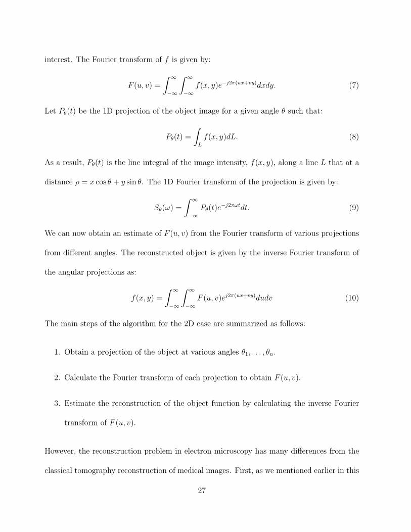
interest. The Fourier transform of f is given by:

F (u, v) =

∫ ∞

−∞

∫ ∞

−∞f(x, y)e−j2π(ux+vy)dxdy. (7)

Let Pθ(t) be the 1D projection of the object image for a given angle θ such that:

Pθ(t) =

∫L

f(x, y)dL. (8)

As a result, Pθ(t) is the line integral of the image intensity, f(x, y), along a line L that at a

distance ρ = x cos θ + y sin θ. The 1D Fourier transform of the projection is given by:

Sθ(ω) =

∫ ∞

−∞Pθ(t)e

−j2πωtdt. (9)

We can now obtain an estimate of F (u, v) from the Fourier transform of various projections

from different angles. The reconstructed object is given by the inverse Fourier transform of

the angular projections as:

f(x, y) =

∫ ∞

−∞

∫ ∞

−∞F (u, v)ej2π(ux+vy)dudv (10)

The main steps of the algorithm for the 2D case are summarized as follows:

1. Obtain a projection of the object at various angles θ1, . . . , θn.

2. Calculate the Fourier transform of each projection to obtain F (u, v).

3. Estimate the reconstruction of the object function by calculating the inverse Fourier

transform of F (u, v).

However, the reconstruction problem in electron microscopy has many differences from the

classical tomography reconstruction of medical images. First, as we mentioned earlier in this

27

paper, electron microscopy images have very low SNR. Second, the image acquisition process

generates a random distribution of projections as the geometry of the data collection cannot

be controlled. Finally, gaps in Fourier space are likely to appear due to uneven distribution

of projection directions. As a result, in order to produce high resolution reconstructions of

the particles, this technique requires the availability of a large number of images of each

particle. This is not always possible as TEM image acquisition is an expensive and time-

consuming process. Additionally, reconstruction of large molecular biological samples can be

computationally demanding, sometimes even requiring the use of special parallel computing

hardware [28].

Mutiple-view epipolar geometry

Alternatively, computer vision methods for multiple-view reconstruction [38, 26] can effec-

tively be applied to the problem of obtaining 3D models from TEM images. The epipolar

geometry constraint [38, 26] allows for the recovery of 3D information from a pair of images

of the same scene or object. Recent work by Brandt et al. [12, 13] has demonstrated the

application of epipolar geometry for the alignment of multiple TEM images. Epipolar geom-

etry has also been used to perform reconstruction of curved nanowires from SEM images [42],

as well as to achieve reconstruction of DNA filaments from TEM images [44]. Cornille et

al. [18] describe a calibration algorithm for 3D reconstruction in SEM images.

The alignment of images taken from different viewing angles is a required step before tomo-

graphic reconstruction can be performed [85]. The method described by Brandt et al. [12, 13]

performs image alignment by means of a global optimization algorithm to solve the feature

28

matching problem over a set of TEM images. Their method starts by finding initial esti-

mates of feature matches from successive images using the epipolar constraint. This is the

stereo matching stage, and it results in a set of point correspondences between each pair of

images. Once these corresponding features are at hand, the method solves for the overall

image alignment by means of a global optimization algorithm [38]. Finally, the aligned im-

ages are used as input for the tomographic reconstruction process. Figure 9 illustrates the

process as a sequence of the above mentioned steps.

Multiple images from various acquisition angles

Feature detection and stereo correspondence

Geometry estimation by optimization over the whole set of images

Reconstructed 3D structure

(a) (b) (c) (d)

Figure 9: A TEM 3D reconstruction system from multiple images. Adapted from [12]. (a)

A set of images from multiple view points. (b) Frame to frame automatic feature match-

ing. (c) Alignment of the feature tracks using epipola constraint. (d) Final tomographic

reconstruction.

Jacob et al. [44] proposed a method to achieve reconstruction of DNA filaments from TEM

images. The method is based on a spline-snake algorithm that minimizes the 3D to 2D

projection error for all views of a cryo-TEM micrographs of a DNA filament. The algorithm

29

requires user initialization of the snake and uses a bank of Gaussian-like directional filters

to detect segments of the DNA filament.

Huang el al. [42] describe a method to reconstruct the 3D shape of curved nanowires. The

method uses epipolar geometry [38, 26] to match stereo pairs of SEM images of nanowires.

The image-formation geometry of electron microscopy can be approximated by orthographic

projection and parallax motion provides enough information for 3D reconstruction. Segments

of the nanowire lying in the epipolar plane cannot be reconstructed. Additionally, the method

works better for nanowires with very low curvature.

The reconstruction of nanoscale objects is a promising problem area for computer vision

applications. Most work so far has focused on the 3D reconstruction process. However,

automatic analysis and recognition of the reconstructed surfaces have not received much at-

tention. Noise and the non-conventional nature of the source data makes these problems even

more challenging and interesting. Next, we present a brief discussion on data visualization

and virtual reality methods applied to the problem of nanoscale characterization.

3.4 Visualization and manipulation

Visualization is crucial to nano-technology. Most of the methods described in this section are

applications of virtual reality for nanoscale visualization. Virtual reality technology provide

an ideal framework to support key applications in nanoscale imaging such as visual inspec-

tion of devices for defect detection as well as precise visual-guided manipulation in device

manufacturing [35, 82, 55]. This can be achieved, for example, by fusing multi-modal imag-

30

ing data and graphics to allow for applications such as device placement and measurement.

Additionally, virtual reality also provides excellent means for education and training [66]. A

recent review of the applications of virtual reality to nanoscale characterization is presented

by Sharma et al. [78].

Fang et al. [24] propose a method for interactive 3D microscopy volumetric visualization.

The method consists of a combination of 2D hardware-supported texture mapping and a

modified fast volume rendering algorithm based on shear-warp of the viewing matrix [51].

Tan et al. [82] describe a nanoscale manipulator system that works with a scanning-probe

microscope (cantilever-based system). The system combines force interaction feedback and

visualization for nanoscale manipulation through a haptic interface.

Figure 10: Broken carbon nano-tube between two raised electrodes [64]

31

Manipulation systems are evolving into immersive virtual reality environments that pro-

vide real-time visual and tactile feedback to the users [55]. This allows for the creation

of nano-devices and sensors in an environment where users can interact with forces and

simultaneously visualize the results of each manipulation.

The development of immersive virtual reality environments is particularly useful in nano-

scale manufacturing. This is the direction taken by the Nanoscale Science Research Group

at UNC-Chapel Hill. They have developed a nanoscale manipulator system that fuses multi-

modal imaging information onto a single visualization output [35]. The system uses projec-

tive texture mapping of SEM image onto AFM topography data along with a calibration

method that allows for localization of the AFM probe in space. The SEM and AFM datasets

are manually aligned and the user can choose the level of relative mixture between the two

data sources.

Basic aspects of virtual reality technology are strongly linked to computer vision techniques

such as camera calibration [93, 83], augmented reality [3], and real-time video-based track-

ing [84, 20]. For instance, image-based tracking can, in principle, be used to provide real-time

feedback for augmented reality tasks while on-line camera calibration methods allow for 3D

alignment of both camera and environment information to support image fusion. Applica-

tions such as nanomotion planning of complex manufacturing tasks implies the integration

of mechanical haptic systems vision-based global planning, and model-based local motion

planing [47].

32

4 Discussion and Conclusions

This paper attempts to provide a comprehensive review of computer vision methods for

image-based nanoscale characterization. The main objective of this paper is to motivate the

development of new computer vision algorithms that will address the many challenges in

this new and promising application area. We have focused mainly on the characterization

and description of the methods without performing quantitative comparisons.

There are several avenues available for future research. Some possible directions include:

• The tracking of particles and surfaces.

• The characterization of noise statistics of nanoscale imaging devices.

• View morphing for visualization when only reduced sets of images are available.

• The development of defect and misalignment detection algorithms.

• The use of texture analysis to characterize nanoscale materials.

• 3D reconstruction using occluding contours and circular motion of the tilting stage.

• The characterization of semi-tranparent objects.

Tracking algorithms are often used in many interesting applications [1, 7, 9]. However, track-

ing is mostly performed at the optical microscope resolution such as fluorescence microscopy

for the analysis of biological specimens. At the nanoscale realm we found the work of Man-

tooth et al. [59], which uses cross-correlation to calculate the drift in scanning tunneling

33

microscope. The algorithm tracks inter-image drift, allowing for registration of an sequence

of images into a single coordinate plane. The detection of defects is another important

application [48].

Modeling image statistics is key to image enhancing. Following a similar approach as the one

proposed by [76], one might attempt to model different levels of noise and image statistics for

specific microscopes and material analysis processes (TEM image acquisition). These models

can be used to help enhance image quality and analyze device structure. Image enhancement

can, in principle, be accomplished through multi-image restoration [15]. This technique

is based on the assumption that multiple images of the same object are often corrupted

by independently-distributed noise [5]. This allows for image restoration algorithms that

combine the information content available in multiple images to obtain a higher quality

image output. This can be of help, for example, for TEM imaging when multiple images are

available but the individual image quality is poor. In this case, multiple image restoration

methods such as the one described in [15] can help produce a better image output.

View-morphing techniques, such as the one developed by Xiao and Shah [89] may help

visualization of nanoscale objects by generating novel views of an object from few image

samples. The generation of novel views provides a way for creating extra geometrically con-

sistent information without the need for explicit 3D reconstruction. For example, generating

TEM images from several view points is a time-consuming and computationally demand-

ing process. View-morphing may reduce the time required for generating novel views by

synthesizing geometrically consistent images from few acquired samples.

34

Tracking [90] and circular motion geometry [45] can be applied to problems such as determin-

ing the spatial localization of particles in nanotube fabrication. The key idea is to analyze

a sequence of TEM images acquired at varying viewing angles. The main problem here is

to determine if particles are present inside or outside of the nanotubes. As TEM images are

projections of the 3D objects, it is difficult to determine the exact location of particles in

the imaged sample.

Nanoscale imaging is certainly an exciting and challenging field with numerous applications

for computer vision research. The low SNR that is a common characteristic of nanoscale

images makes the application of vision techniques even more challenging. However, as vision

algorithms become more robust and available computer hardware becomes faster, we are

able to approach these problems more successfully. In terms of advancing computer vision

technology, the challenging aspects of nanoscale image provide an excellent testbed that will

drive vision algorithms to become increasingly more robust and accurate.

References

[1] F. Aguet, D. Van De Ville, and M. Unser. Sub-resolution axial localization of nanoparti-

cles in fluorescence microscopy. In T. Wilson, editor, Proceedings of the SPIE European

Conference on Biomedical Optics: Confocal, Multiphoton, and Nonlinear Microscopic

Imaging II (ECBO’05), volume 5860, pages 103–106, Munich, Germany, June 12–16,

2005.

35

[2] F. Aurenhammer. Voronoi diagrams – a survey of a fundamental geometric data struc-

ture. ACM Comput. Surv., 23(3):345–405, 1991.

[3] R. Azuma. A survey of augmented reality. Presence: Teleoperators and Virtual Envi-

ronment, 6(4):355–385, 1997.

[4] J. Banks, R. Rothnagel, and B. Hankamer. Automated particle picking of biological

molecules images by electron microscopy. In Image and Vision Computing New Zealand,

pages = 269–274, November 2003.

[5] M. Belge, M. Kilmer, and E. Miller. Wavelet domain image restoration with adaptive

edge-preserving regularization. IP, 9(4):597–608, April 2000.

[6] D. Bera, S.C. Kuiry, M. McCutchen, A. Kruize, H. Heinrich, S. Seal, and M. Meyyappan.

In-situ synthesis of palladium nanoparticles-filled carbon nanotubes using arc discharge

in solution. Chemical Physics Letters, 386(4–6):364–368, 2004.

[7] A. J. Berglund and H. Mabuchi. Tracking-fcs: Fluorescence correlation spectroscopy of

individual particles. Optical Express, 13:8069–8082, 2005.

[8] M. J. Black, G. Sapiro, D. Marimont, and D. Heeger. Robust anisotropic diffusion.

IEEE Transactions on Image Processing, 7(3):421–432, 1998.

[9] S. Bonneau, M. Dahan, and L. D. Cohen. Single quantum dot tracking based on per-

ceptual grouping using minimal paths in a spatiotemporal volume. IEEE Transactions

on Image Progressing, 14(9):1384–1395, 2005.

36

[10] A. C. Bovik, J. D. Gibson, and A. Bovik, editors. Handbook of Image and Video

Processing. Academic Press, Inc., Orlando, FL, USA, 2000.

[11] R. Bracewell. The Fourier Transform and Its Applications. McGraw-Hill, 3rd ed., New

York, 1999.

[12] S. Brandt, J. Heikkonen, and P. Engelhardt. Automatic alignment of transmission

electron microscope tilt series without fiducial markers. Journal of Structural Biology,

136:201–213, 2001.

[13] S. Brandt, J. Heikkonen, and P. Engelhardt. Multiphase method for automatic align-

ment of transmission electron microscope images using markers. Journal of Structural

Biology, 133(1):10–22(13), January 2001.

[14] L. G. Brown. A survey of image registration techniques. ACM Computer Survey,

24(4):325–376, 1992.

[15] Y. Chen, H. Wang, T. Fang, and J. Tyan. Mutual information regularized bayesian

framework for multiple image restoration. In IEEE International Conference on Com-

puter Vision (ICCV), 2005.

[16] Y. K. Chen, A. Chu, J. Cook, M. L. H. Green, P. J. F. Harris, R. Heesom, M. Humphries,

J. Sloan, S. C. Tsang, and J. F. C. Turner. Synthesis of carbon nanotubes containing

metal oxides and metals of the d-block and f-block transition metals and related studies.

Journal of Materials Chemistry, 7(3):545 – 549, 1997.

37

[17] V. Comaniciu and P. Meer. Kernel-based object tracking. IEEE Transactions on Pattern

Analysis and Machine Intelligence 25, May 2003, 25(5):564–575, 2003.

[18] N. Cornille, D. Garcia, M. Sutton, S. McNeil, and J. Orteu. Automated 3-D reconstruc-

tion using a scanning electron microscope. In SEM Annual Conf. & Exp. on Experi-

mental and Applied Mechanics, 2003.

[19] A. Dempster, N.M. Laird, and D.B. Rubin. Maximum likelihood from incomplete data

via the EM algorithm. Journal Royal Statistical Society, Series B, 39(1):1–38, 1977.

[20] T. Drummond and R. Cipolla. Real-time tracking of complex structures with on-line

camera calibration. Image Vision Comput., 20(5-6):427–433, 2002.

[21] R. O. Duda and P. E. Hart. Use of the hough transformation to detect lines and curves

in pictures. Communications of ACM, 15(1):11–15, 1972.

[22] M. R. Falvo, G. Clary, A. Helser, S. Paulson, R. M. Taylor II, V. Chi, F. P. Brooks Jr,

S. Washburn, and R. Superfine. Nanomanipulation experiments exploring frictional and

mechanical properties of carbon nanotubes. Microscopy and Microanalysis, 4:504–512,

1998.

[23] M. R. Falvo, R. M. Taylor II, A. Helser, V. Chi, F. P. Brooks Jr, S. Washburn, and

R. Superfin. Nanometre-scale rolling and sliding of carbon nanotubes. Nature, 397:236–

238, 1999.

[24] S. Fang, Y. Dai, F. Myers, M. Tuceryan, and K. Dunn. Three-dimensional microscopy

data exploration by interactive volume visualization. Scanning, 22:218–226, 2000.

38

[25] M. Farabee. On-line biology book. (http://www.emc.maricopa.edu/faculty/

farabee/BIOBK/BioBookTOC.html), 2001.

[26] O. Faugeras. Three-dimensional computer vision: a geometric viewpoint. MIT Press,

1993.

[27] J. Fernandez, A. Lawrence, J. Roca, I. Garcia, M. Ellisman, and J. Carazo. High-

performance electron tomography of complex biological specimens. J. Structural Biol.,

138:6–20, 2002.

[28] J.-J. Fernandez, J.-M. Carazo, and I. Garcia. Three-dimensional reconstruction of cel-

lular structures by electron microscope tomography and parallel computing. J. Parallel

Distrib. Comput., 64(2):285–300, 2004.

[29] S. L. Flegler, J. W. Heckman, and K. L. Klomparens. Scanning and Transmission

Electron Microscopy: An Introduction. Oxford Press, 1995.

[30] J. Gallop. SQUIDs: some limits to measurement. Superconductor Science and Technol-

ogy, 16:1575–1582, 2003.

[31] Y. Garini, B. J. Vermolen, and I. T. Young. From micro to nano: recent advances in

high-resolution microscopy. Current Opinion in Biotechnology, 16(3):3–12, 2005.

[32] J. I. Goldstein, D. E. Newbury, P. Echlin, D. C. Joy, C. Fiori, and E. Lifshin. Scan-

ning Electron Microscopy and X-Ray Microanalysis: A Text for Biologists, Materials

Scientists, and Geologists. Plenum Publishing Corporation, 1981.

39

[33] U. Grenander and A. Srivastava. Probability models for clutter in natural images. IEEE

Transactions on Pattern Analysis and Machine Intelligence., 23(4):424–429, 2001.

[34] C. L. Grimellec, E. Lesniewska, M.-C. Giocondi, E. Finot, V. Vie, and J.-P. Goudonnet.

Imaging of the surface of living cells by low-force contact-mode atomic force microscopy.

Biophysical Journal, 75:695–703, 1998.

[35] M. Guthold, W. Liu, B. Stephens, S. T. Lord, R. R. Hantgan, D. A. Erie, R. M. Taylor

II, and R. Superfine. Visualization and mechanical manipulations of individual fibrin

fibers. Biophysical Journal, 87(6):4226–4236, 2004.

[36] R. M. Haralick and L. G. Shapiro. Computer and Robot Vision. Addison-Wesley Long-

man Publishing Co., Inc., Boston, MA, USA, 1992.

[37] G. Harauz and A. Fong-Lochovsky. Automatic selection of macromolecules from elec-

tron micrographs by component labelling and symbolic processing. Ultramicroscopy.,

31(4):333–44., 1989.

[38] R. I. Hartley and A. Zisserman. Multiple View Geometry in Computer Vision. Cam-

bridge University Press, 2000.

[39] M. Heiler and C. Schnorr. Natural image statistics for natural image segmentation.

International Journal of Computer Vision, 63(1):5–19, 2005.

[40] S. W. Hell. Towards fluorescence nanoscopy. Nature Biotechnology, 21(11):1347–1355,

2003.

40

[41] B. Horn. Robot Vision. MIT Press, Cambridge, Massachusetts, 1986.

[42] Z. Huang, D. A. Dikin, W. Ding, Y. Qiao, X. Chen, Y. Fridman, and R. S. Ruoff. Three-

dimensional representation of curved nanowires. Journal of Microscopy, 216(3):206–214,

2004.

[43] S. J. Ludtke, P. Baldwin, and W. Chiu. Eman: semiautomated software for high-

resolution single-particle reconstructions. Journal of Structural Biology, 128:82–97,

1999.

[44] M. Jacob, T. Blu, and M. Unser. 3-D reconstruction of DNA filaments from stereo

cryo-electron micrographs. In Proceedings of the First 2002 IEEE International Sym-

posium on Biomedical Imaging: Macro to Nano (ISBI’02), volume II, pages 597–600,

Washington DC, USA, July 7–10, 2002.

[45] G. Jiang, L. Quan, and H.-T. Tsui. Circular motion geometry using minimal data. IEEE

Transactions on Pattern Analysis and Machine Intelligence., 26(6):721–731, 2004.

[46] C. Kammerud, B. Abidi, and M. Abidi. Computer vision algorithms for 3D reconstruc-

tion of microscopic data - a review. Microscopy Microanalysis, 11:636–637, 2005.

[47] D.-H. Kim, T. Kim, , and B. Kim. Motion planning of an afm-based nanomanipulator in

a sensor-based nanorobotic manipulation system. In Proceedings of 2002 International

Workshop on Microfactory, pages = 137–140, 2002.

41

[48] T. Kubota, P. Talekar, X. Ma, and T. S. Sudarshan. A non-destructive automated

defect-detection system for silicon carbide wafers. Machine Vision and Applications,

16(3):170–176, 2005.

[49] S. Kumar, K. Chaudhury, P. Sen, and S. K. Guha. Atomic force microscopy: a powerful

tool for high-resolution imaging of spermatozoa. Journal of Nanobiotechnology, 3(9),

September 2005.

[50] S. Kumar and M. Hebert. Discriminative fields for modeling spatial dependencies in

natural images. In Proceedings of Advances in Neural Information Processing Systems

(NIPS), December 2003.

[51] P. Lacroute and M. Levoy. Fast volume rendering using a shear-warp factorization of the

viewing transformation. In SIGGRAPH ’94: Proceedings of the 21st Annual Conference

on Computer Graphics and Interactive Techniques, pages 451–458, New York, NY, USA,

1994. ACM Press.

[52] J. H. Lambert. Photometria sive de mensure de gratibus luminis, colorum umbrae.

Eberhard Klett, 1760.

[53] A. B. Lee, K. S. Pedersen, and D. Mumford. The nonlinear statistics of high-contrast

patches in natural images. International Journal of Computer Vision, 54(1-3):83–103,

2003.

[54] Z. H. Levine, A. R. Kalukin, M. Kuhn, C. C. R. Sean P. Frigo, Ian McNulty, Y. Wang,

T. B. Lucatorto, B. D. Ravel, and C. Tarrio. Tomography of integrated circuit inter-

42

connect with an electromigration void. Journal of Applied Physics, 87(9):4483–4488,

2000.

[55] G. Li, N. Xi, M. Yu, and W.-K. Fung. Development of augmented reality system for

afm-based nanomanipulation. IEEE/ASME Transactions on Mechatronics, 9(2):358–

365, 2004.

[56] S. Z. Li. Markov random field modeling in computer vision. Springer-Verlag, London,

UK, 1995.

[57] V. Lucic, F. Forster, and W. Baumeister. Structural studies by electron tomography:

From cells to molecules. Annual Review of Biochemistry, 74:833–865, 2005.

[58] S. P. Mallick, Y. Xu, and D. J. Kriegman. Detecting particles in cryo-em micrographs

using learned features. Journal of Structural Biology, Volume 145(1-2):52–62, Jan/Feb

2004.

[59] B. A. Mantooth, Z. J. Donhauser, K. F. Kelly, and P. S. Weiss. Cross-correlation image

tracking for drift correction and adsorbate analysis. Review of Scientific Instruments,

73:313–317, Feb. 2002.

[60] S. Marco, T. Boudier, C. Messaoudi, and J.-L. Rigaud. Electron tomography of biolog-

ical samples. Biochemistry (Moscow), 69(11):1219–1225, 2004.

[61] G. J. McLachlan and D. Peel. Robust cluster analysis via mixtures of multivariate

t-distributions. In SSPR/SPR, pages 658–666, 1998.

43

[62] W. V. Nicholson and R. M. Glaeser. Review: automatic particle detection in electron

microscopy. Journal of Structural Biology, 133:90–101, 2001.

[63] W. V. Nicholson and R. Malladi. Correlation-based methods of automatic particle de-

tection in electron microscopy images with smoothing by anisotropic diffusion. Journal

of Microscopy, 213:119–128, 2004.

[64] NSRG-Chappel Hill. Nanoscale-Science Research Group. http: // www. cs. unc. edu/

Research/ nano/ , 2005.

[65] T. Ogura and C. Sato. An automatic particle pickup method using a neural network ap-

plicable to low-contrast electron micrographs. Journal of Structure Biology, 136(3):227–

238, 2001.

[66] E. W. Ong, A. Razdan, A. A. Garcia, V. B. Pizziconi, B. L. Ramakrishna, and W. S.

Glaunsinger. Interactive nano-visualization of materials over the internet. Journal of

Chemical Education, 77(9):1114–1115, 2000.

[67] P. Perona and J. Malik. Scale-space and edge detection using anisotropic diffusion.

IEEE Transactions on Pattern Analysis and Machine Intelligence, 12(7):629–639, 1990.

[68] D. W. Pohl. Scanning near-field optical microscopy, volume 12 of Advances in Optical

and Electron Microscopy. C. J. R. Sheppard and T. Mulvey, Eds. Academic Press,

London, 1990.

[69] O. Ronneberger, E. Schultz, and H. Burkhardt. Automated pollen recognition using 3D

volume images from fluorescence microscopy. Aerobiologia, 18(2):107–115, 2002.

44

[70] A. Rosenfeld and J. Pfaltz. Distance functions on digital pictures. Pattern Recognition,

1(1):33–61, July 1968.

[71] D. Rugar, R. Budakian, H. J. Mamin, and B. W. Chui. Single spin detection by magnetic

resonance force microscopy. Nature, 430, July 2004.

[72] J. C. Russ. The Image Processing Handbook. IEEE Press, 1998.

[73] J. Ryu, B. K. P. Horn, M. S. Mermelstein, S. Hong, and D. M. Freedam. Application of

structured illumination in nanoscale vision. In Proceedings of IEEE Computer Society

Conference on Computer Vision and Pattern Recognition Workshop: Computer Vision

for the Nano Scale, pages = 17–24, June 2003.

[74] K. Sandberg, D. N. Mastronarde, and G. Beylkina. A fast reconstruction algorithm for

electron microscope tomography. Journal of Structural Biology, 144:6172, 2003.

[75] H. Scharr, M. Black, and H. Haussecker. Image statistics and anisotropic diffusion. In

ICCV03, pages 840–847, 2003.

[76] H. Scharr, M. Felsberg, and P.-E. Forssen. Noise adaptive channel smoothing of low-

dose images. In Proceedings of IEEE Computer Society Conference on Computer Vision

and Pattern Recognition Workshop: Computer Vision for the Nano Scale, June 2003.

[77] H. Scharr and D. Uttenweiler. 3d anisotropic diffusion filtering for enhancing noisy actin

filament fluorescence images. In Proceedings of the 23rd DAGM-Symposium on Pattern

Recognition, pages 69–75, London, UK, 2001. Springer-Verlag.

45

[78] G. Sharma, C. Mavroidis, and A. Ferreira. Virtual Reality and Haptics in Nano and

Bionanotechnology, volume X of Handbook of Theoretical and Computational Nanotech-

nology, chapter 40. American Scientific Publishers, 2005.

[79] V. Singh, D. C. Marinescu, and T. S. Baker. Image segmentation for automatic particle

identification in electron micrographs based on hidden markov random field models and

expectation maximization. Journal of Structural Biology, 145(1-2):123–141, January

2004.

[80] A. Stoscherk and R. Hegerl. Automated detection of macromolecules from electron

micrographs using advanced filter techniques. Journal of Microscopy, 185:76–84, 1997.

[81] S. Subramaniam and J. L. Milne. Three-dimensional electron microscopy at molecular

resolution. Annual Review of Biophysics and Biomolecular Structure, 33:141–155, 2004.

[82] H. Z. Tan, L. Walker, R. Reifenberger, S. Mahadoo, G. Chiu, A. Raman, A. Helser, and

P. Colilla. A haptic interface for human-in-the-loop manipulation at the nanoscale. In

Proceedings of the 2005 World Haptics Conference (WHC05): The First Joint Euro-

Haptics Conference and the Symposium on Haptic Interfaces for Virtual Environment

and Teleoperator Systems, pages 271–276, 2005.

[83] R. Y. Tsai. A versatile camera calibration technique for high-accuracy 3D machine

vision metrology using off-the-shelf TV cameras and lenses. IEEE Journal Robotics

Automation, RA-3(4):323–344, 1987.

46

[84] A. Valinetti, A. Fusiello, and V. Murino. Model tracking for video-based virtual reality.

In ICIAP, pages 372–377, 2001.

[85] M. van Heel, B. Gowen, R. Matadeen, E. V. Orlova, R. Finn, T. Pape, D. Cohen,

H. Stark, R. Schmidt, M. Schatz, and A. Patwardhan. Single-particle electron cryo-

microscopy : towards atomic resolution. Quarterly Reviews of Biophysics, 33(4):307–

369, 2000.

[86] P. Viola and M. J. Jones. Robust real-time face detection. International Journal of

Computer Vision, 57(2):137–154, 2004.

[87] I. M. Watt. The Principles and Practice of Electron Microscopy. Cambridge, 1997.

[88] J. Weickert. Anisotropic Diffusion in Image Processing. Teubner Verlag, 1997.

[89] J. Xiao and M. Shah. Tri-view morphing. Computer Vision and Image Understanding,

2004.

[90] A. Yilmaz, K. Shafique, and M. Shah. Target tracking in airborne forward looking

infrared imagery. Image and Vision Computing, 21(7):623–635, 2003.

[91] Z. Yu and C. Bajaj. A gravitation-based clustering method and its applications in 3D

electron microscopy imaging. In 5th International Conference on Advances in Pattern

Recognition(ICAPR’03), pages = 137–140, 2003.

47

[92] Z. Yu and C. Bajaj. Detecting circular and rectangular particles based on geometric

feature detection in electron micrographs. Journal of Structural Biology, 145:168180,

2004.

[93] Z. Zhang. A flexible new technique for camera calibration. IEEE Transactions on

Pattern Analysis and Machine Intelligence., 22(11):1330–1334, 2000.

[94] Y. Zhu, B. Carragher, R. M. Glaeser, D. Fellmann, C. Bajaj, M. Bern, F. Mouche,

F. de Haas, R. J. Hall, D. J. Kriegman, S. C. Ludtke, S. P. Mallick, P. A. Penczek,

A. M. Roseman, F. J. Sigworth, N. Volkmann, and C. S. Potter. Automatic particle

selection: Results of a comparative study. Journal of Structural Biology, 145:3–14, 2004.

[95] Y. Zhu, B. Carragher, D. Kriegman, R. A. Milligan, and C. S. Potter. Automated

identification of filaments in cryoelectron microscopy images. Journal of Structural

Biology, 135:302–321, 2001.

[96] Y. Zhu, B. Carragher, F. Mouche, and C. S. Potter. Automatic particle detec-

tion through efficient Hough transforms. IEEE Transactiona on Medical Imaging,

22(9):1053–1062, 2003.

48