computer simulation of adaptive bone remodeling simulation of adaptive bone remodeling ... of this...
TRANSCRIPT

Computer simulation of adaptive boneremodeling
Thomas RubergTechnische Universitat Braunschweig
Centro Polictecnico Superior Zaragoza

CONTENTS CONTENTS
Contents
1 Introduction 3
2 Bone structure 42.1 Bone tissue . . . . . . . . . . . . . . . . . . . . . . . . . . . . 52.2 Composition of bone . . . . . . . . . . . . . . . . . . . . . . . 82.3 Bone cells . . . . . . . . . . . . . . . . . . . . . . . . . . . . . 102.4 Mineralization . . . . . . . . . . . . . . . . . . . . . . . . . . . 112.5 Mechanical features . . . . . . . . . . . . . . . . . . . . . . . . 122.6 Damage in bone . . . . . . . . . . . . . . . . . . . . . . . . . . 15
3 Bone remodeling 193.1 Basic observations . . . . . . . . . . . . . . . . . . . . . . . . 193.2 Wolff’s law and the concept of remodeling . . . . . . . . . . . 213.3 Basic multicellular units . . . . . . . . . . . . . . . . . . . . . 223.4 Purpose and origination . . . . . . . . . . . . . . . . . . . . . 25
4 Computational models 284.1 Adaptive elasticity . . . . . . . . . . . . . . . . . . . . . . . . 284.2 Mechanical approach . . . . . . . . . . . . . . . . . . . . . . . 29
4.2.1 History . . . . . . . . . . . . . . . . . . . . . . . . . . . 294.2.2 The isotropic Stanford model . . . . . . . . . . . . . . 314.2.3 Anisotropic extension . . . . . . . . . . . . . . . . . . . 374.2.4 Enhancement proposed by Garcıa and Doblare . . . . . 414.2.5 Revision . . . . . . . . . . . . . . . . . . . . . . . . . . 46
4.3 Phenomenological approach . . . . . . . . . . . . . . . . . . . 474.3.1 The method of Hazelwood, Martin et al. . . . . . . . . 484.3.2 The method of Hernandez . . . . . . . . . . . . . . . . 54
4.4 Discussion . . . . . . . . . . . . . . . . . . . . . . . . . . . . . 58
5 Proposition of a new model 605.1 Definition of internal scalar variables . . . . . . . . . . . . . . 615.2 Resorption and formation . . . . . . . . . . . . . . . . . . . . 635.3 Mineralization . . . . . . . . . . . . . . . . . . . . . . . . . . . 705.4 Damage . . . . . . . . . . . . . . . . . . . . . . . . . . . . . . 725.5 Extension to anisotropy . . . . . . . . . . . . . . . . . . . . . 75
6 Numerical evaluation 796.1 Validation of the model . . . . . . . . . . . . . . . . . . . . . . 796.2 THR-prosthesis . . . . . . . . . . . . . . . . . . . . . . . . . . 85
1
CONTENTS CONTENTS
7 Outlook 89
Appendix 90
A Basic concepts of continuum damage mechanics 90
B Fabric tensor 93
C FEM-model of the proximal femur 95
D Algorithms 98
List of Figures 102
List of Tables 103
References 104
This document was authored using LATEX2ε. Function plots have been produced withMATLAB 6.2 , and pictures have been created with Xfig 3.2 . Calculations have beenperformed on standard personal computers with ABAQUS 6.2.7 using subroutines inFORTRAN - and C -codes. Data visualization was done with the CAE-Viewer of thesame ABAQUS -package or MATLAB.
2
1 INTRODUCTION
1 Introduction
Bone is a living material which has its main function in forming the skeletonand therefore enabling locomotion and protection of the organism. It is sub-jected to permanent and transient loads caused by the daily active or specialevents like accidents. On the contrary to inert materials from standard me-chanics, this tissue is able to respond adaptively to its environment. Apartfrom skeletal growth and fracture healing, which are of temporary character,the internal structure of bone is maintained and adapted internally by anenduring process, termed remodeling.
This process is assumed to remove microdamage and thereby increasethe fatigue lifetime of the tissue. Furthermore, the structural adaptation tochanges in the mechanical environment plays an important role in the contextof implants and prostheses. In fact, latest developments of such devices havebeen analyzed numerically in order to estimate the long-term reaction of thetissue to this impact. Another item are bone diseases, especially osteoporosis ,which underly similar concepts as the remodeling process. Due to the hugesocial damage caused by such diseases and failure of implants and prostheses,an advance in the understanding and computer simulation of remodeling isof great importance.
Therefore, this phenomenon has been gaining increasing interest in thelast century. Especially in the last twenty years, many numerical algorithmshave been developed in order to simulate this process. Although early modelswere capable of predicting good approaches to the real behavior, a quantita-tive analysis has been impossible and many biologic aspects have been ne-glected. Recently, new methods have been published which take into accountaspects of the microstruture and cell activities. These models provide goodresults for predictions of bone loss due to osteoporosis but suffer deficienciesfrom a mechanical point of view.
After introducing the whole matter and reviewing some of the importantmodels for computer simulations, a new model will be developed in this work.It follows the line of previously published methods but combines mechanicaland biological aspects and will be adjusted to experimental findings in orderto go a step further in the direction of a reliable algorithm.
In the following, the micro- and macrostructure of this tissue will be de-scribed in chapter 2.1 together with mechanically important items as miner-alization and damage. Afterwards the process of remodeling will be outlinedin chapter 3. Some important numerical models on this process are presentedthen in chapter 4. The theoretical part of the new model is given in chap-ter 5, whereas chapter 6 is dedicated to its numerical evaluation. Finally, aconclusion is made in 7 and the appendix provides some specific details.
3

2 BONE STRUCTURE
Fig. 2.1. Left: human skeleton with appellation of some bones, from Carter and Beaupre,2001. Right: geometry of a typical long bone, from Garcıa, 1999.
2 Bone structure
In this chapter, the basic features of bone as a biological tissue under me-chanical circumstances will be outlined. After describing the shapes andtypes in 2.1, the composition of bone is presented in 2.2 and its cells -theactuators of bone dynamics- are introduced in 2.3. A mechanically impor-tant property, the degree of mineralization, results from the mineralizationprocess, explained in 2.4. Finally, the mechanical behavior, i.e., bone as asolid structure, will be described in 2.5 followed by some comments on fatiguedamage in 2.6.
4

2 BONE STRUCTURE 2.1 Bone tissue
2.1 Bone tissue
In general, the shape of bones can be classified into three groups: short, flat,and long. Whereas short bones (e.g. the calcaneus in the heel) have similarextensions in all dimensions, flat bones (cranium, shoulder blade) have onedimension much shorter than the other two and long bones (femur, tibia,ulna) one dimension much longer. Long bones have a primarily structuralfunction and flat bones are mainly protective. But all bone types alwayshave both functions. Additionally, there are irregular bones which can notbe identified as a member of one of these classes. A typical example arethe vertebrae in the spinal. The left image of figure 2.1 depicts the humanskeleton and thus examples for each kind of bone (cf. Buckwalter et al., 1995,and Martin et al., 1998, for more details on this and the subsequent items).
A long bone can be described geometrically relative to its physis whichis the ’scar’ left from the growth plate after the adolescence, as shown in theright picture of figure 2.1. The physis is located in a relative short distance tothe end of the bone and the part between the end and the physis is termedepiphysis . The region on the other side of the physis is called metaphysiswhich is the boundary to the middle part, the diaphysis.
The above given examples in parentheses do not necessarily refer to hu-man bones but can be found in any other animal having a vertebrate skeleton.This work will concentrate on long bones of the limbs and take the humanfemur as the classical example for remodeling theories. This is mainly donefor the reason that this bone is of high interest in orthopeadic surgery sinceboth knee and hip joint prostheses affect on it and are themselves the mostimportant examples of such devices. Another reason, which has evidently thesame origin, is the huge number of available data on this specimen. In par-ticular, the presented methods will only be applied to the proximal† femur.This reduction does not exclude any other bone type from the theoreticalanalysis and the applied hypotheses are supposed to hold for any kind ofosteonal structure.
Changing to a microscale the terms describing the shape or the positionof the bone do not apply anymore. There are just two different kinds ofbone tissue: cortical and trabecular , easily distinguished by their degree ofporosity. The bone tissue of both kinds is surrounded by marrow, which
†The term proximal refers to the part which is closer to the head, whereas distal isfurther from the head, i.e., the proximal femur includes the region of the hip joint and thepart above the knee is the distal femur.Furthermore, the terms lateral and medial referto parts which are further or closer to a plane through the central axis of the body andextending to the front and back. Therefore, the region of the femur away from the centerof body is lateral whereas the inner region is medial.
5

2 BONE STRUCTURE 2.1 Bone tissue
serves as a source of bone cells and contains blood vessels and nerves. Mar-row is present in every known bone (except for the ossicles of the inner ear)and cannot exist outside the skeleton. There are two kinds of marrow, fattyand hematopoietic (also termed yellow and red), where the latter one formsan indispensable part in blood production. Marrow will not be consideredfurthermore and is assumed not to influence directly on the mechanical be-havior of bone. There is investigation dedicated to bone as a poroelasticmaterial and thus taking into account marrow as the pore fluid. But it israther doubtful, whether such a detailed description benefits in the contextof bone remodeling.
One can state that a given volume of bone consists of two parts
VT = VB + VV , (2.1)
where the indices T , B and V refer to the total, bone tissue and void partsof the volume, respectively. Note the distinction between bone, which cor-responds to the total volume VT , and bone tissue, which does not containmarrow or void. With this definition of the volume parts the term porositycan be determined
p = VV /VT = 1− VB/VT . (2.2)
Another important, but easily related quantity is the apparent density ρdescribed by
ρ = mT/VT = (mB +mV )/VT , (2.3)
which is generally reduced to
p = 1− ρ/ρt (2.4)
by assigning zero mass to the void volume, where ρt = mB/VB refers to thebone tissue density. The tissue density ρt is thus the density of an imaginarybone specimen without porosity. This quantity is generally assumed to bea constant value about 2.0 g/cm3, but considering mineralization makes itvariable (cf. section 2.4). The quotient VB/VT is often referred to as thebone volume fraction and plays an important role concerning the mechanicalproperties of bone.
With these terms, the above mentioned tissue types can be classified.Trabecular bone (often referred to as cancellous or spongy bone) is a veryporous structure which is found in short and flat bones as well as in theends of long bones. Its high porosity usually varies between 0.75 and 0.95.The pores are interconnected and filled with marrow and the mineralizedmatrix is made up of the strut- or plate-like formed trabeculae, which are
6
2 BONE STRUCTURE 2.1 Bone tissue
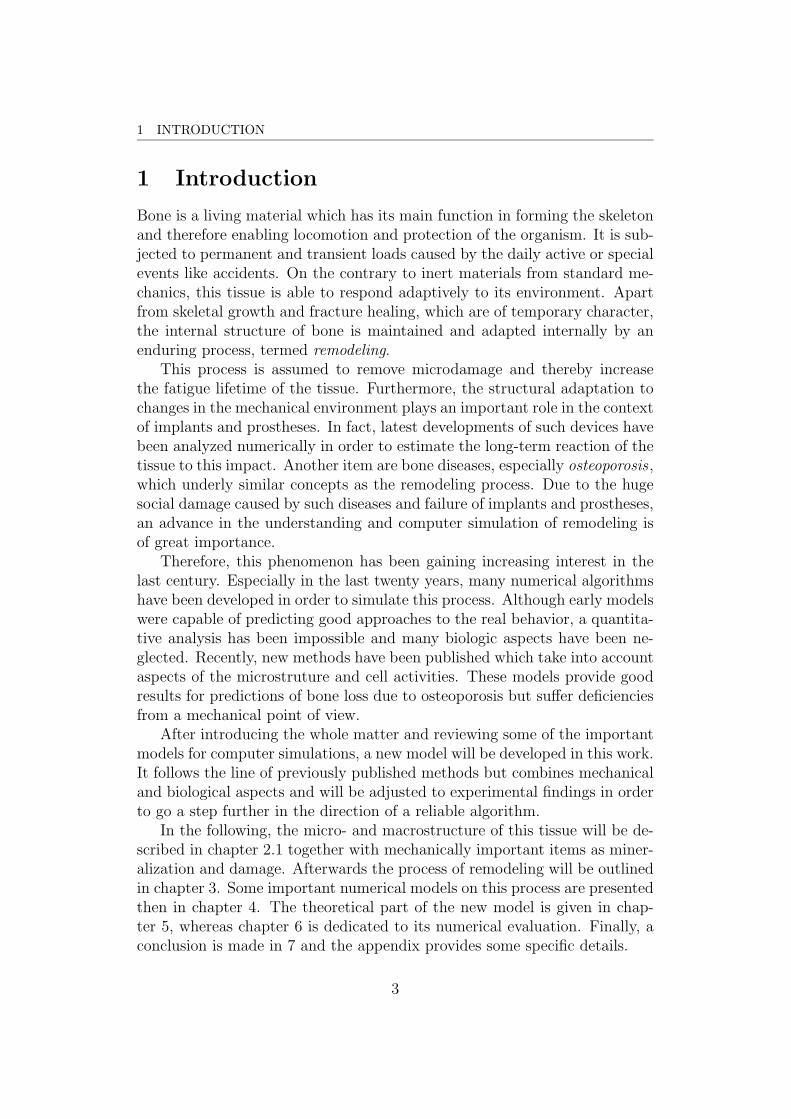
Fig. 2.2. Photographs of the two tissue types: trabecular and cortical. Taken from Martinet al., 1998.
about 200µm thick. The example in the left image of figure 2.2 might givean impression, how the trabecular bone is constructed.
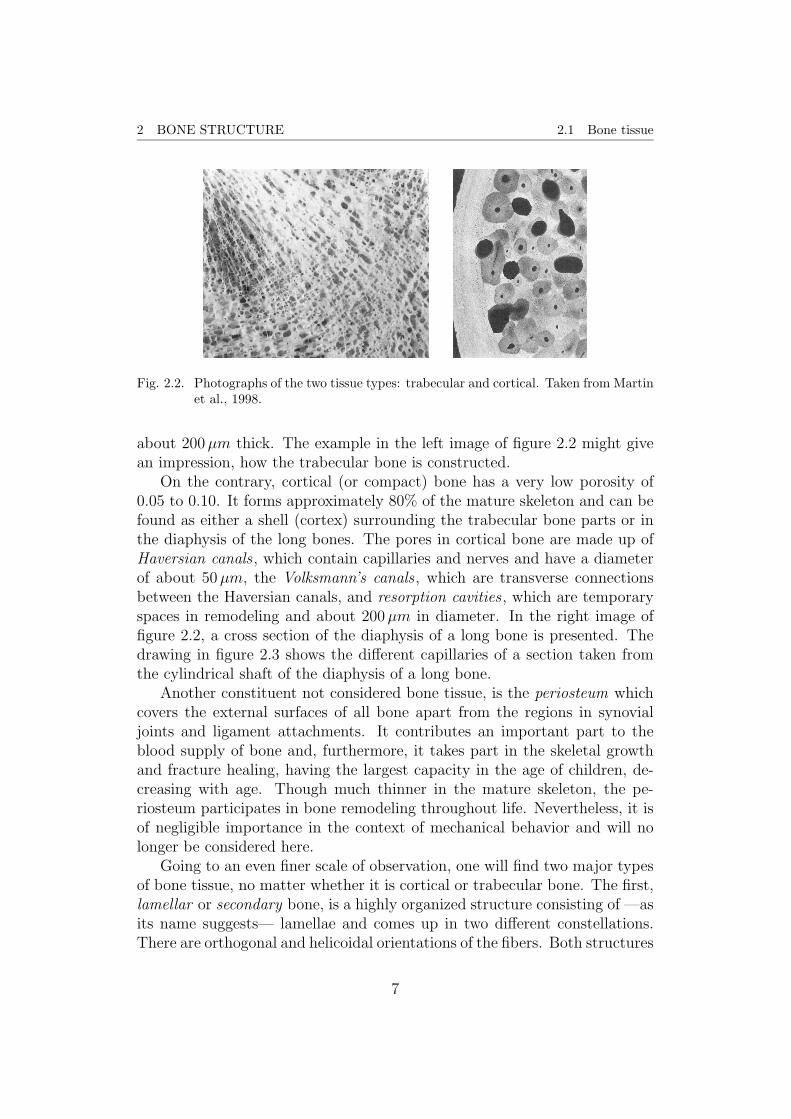
On the contrary, cortical (or compact) bone has a very low porosity of0.05 to 0.10. It forms approximately 80% of the mature skeleton and can befound as either a shell (cortex) surrounding the trabecular bone parts or inthe diaphysis of the long bones. The pores in cortical bone are made up ofHaversian canals , which contain capillaries and nerves and have a diameterof about 50µm, the Volksmann’s canals , which are transverse connectionsbetween the Haversian canals, and resorption cavities , which are temporaryspaces in remodeling and about 200µm in diameter. In the right image offigure 2.2, a cross section of the diaphysis of a long bone is presented. Thedrawing in figure 2.3 shows the different capillaries of a section taken fromthe cylindrical shaft of the diaphysis of a long bone.
Another constituent not considered bone tissue, is the periosteum whichcovers the external surfaces of all bone apart from the regions in synovialjoints and ligament attachments. It contributes an important part to theblood supply of bone and, furthermore, it takes part in the skeletal growthand fracture healing, having the largest capacity in the age of children, de-creasing with age. Though much thinner in the mature skeleton, the pe-riosteum participates in bone remodeling throughout life. Nevertheless, it isof negligible importance in the context of mechanical behavior and will nolonger be considered here.
Going to an even finer scale of observation, one will find two major typesof bone tissue, no matter whether it is cortical or trabecular bone. The first,lamellar or secondary bone, is a highly organized structure consisting of —asits name suggests— lamellae and comes up in two different constellations.There are orthogonal and helicoidal orientations of the fibers. Both structures
7
2 BONE STRUCTURE 2.2 Composition of bone
Fig. 2.3. A drawing of the composition of cortical bone. Taken from Martin et al., 1998.
are present in human bone. Due to its plywood-like structure, lamellar bonehas a relative high resistance but needs a significant time to be built.
Much weaker but quicker formed is the second type, the woven or primarybone. Its arrangement can be considered random. This tissue plays animportant role in fracture healing since it can quickly connect the separatedparts. Furthermore, it forms the embryonic skeleton and appears primarilyin the growth plate. Apart from these and some other exceptions, it rarelyis present in a normal human skeleton after the first years of life.
2.2 Composition of bone
Bone tissue or matrix consists of organic and inorganic components. Theorganic part (also referred to as osteoid) contributes about 20% of totalmass and contains mainly collagen. 65% are inorganic or mineral and watermakes up another 10% (Buckwalter et al., 1995; Martin et al., 1998).
Collagen is a protein which can organize itself into fibers. Many variantsof collagen are known, but type I is predominant in mature bone. It gives thematrix its flexibility and tensile strength and provides location for mineral
8

2 BONE STRUCTURE 2.2 Composition of bone
crystals. The non-collagenous part of the organic matrix is supposed tohave a high influence on bone-cell function rather than on the mechanicalproperties of the tissue.
The mineral phase gives bone most of its stiffness and compressive strengthand serves as an ion reservoir. The latter feature has its function even apartfrom the skeleton and is important for the metabolism of the whole body.In the current context more important, it forms together with the organicmatrix a rigid material which withstands the forces due to normal activ-ity. This mineral constituent is mainly made of hydroxyapatite crystals(Ca10(PO4)6(OH)2) also known as dahlite (Buckwalter et al., 1995). It ap-pears in a relative impure constitution which varies with age. The crystalsitself are rod-like shaped with a size of 5× 5× 40 nanometer. The formationof the inorganic matrix happens due to the process of mineralization whichwill be described later.
This composite structure itself is porous. Its voids, termed lacunae, aremicroscopically small spaces which are connected by canaliculi and provideloci for bone cells. One cubic millimeter bone tissue contains up to 15,000lacunae (Hernandez, 2001). This kind of porosity will not be taken intoaccount in the following analysis and shall not be confused with the boneporosity determined by the void volume VV .
The water content is partially bonded to collagen. But free water appearsas well and takes part in the mineralization process.
In terms of its composition, a given bone tissue volume can be analyzedas follows
VB = VO + VM + VW ,
where the indices O, M , and W indicate the organic, inorganic or mineral,and water constituents, respectively. A dried specimen of bone has the drymass , md = mO +mM , and, after being in the furnace in order to evaporatethe organic parts, only the mass fraction mM will remain. To measure thedegree of mineralization the ash fraction is used
α = mM/md , (2.5)
which typically is about 0.65 (Martin et al., 1998).Like marrow in the void volume, the water part will be neglected as well.
It does not significantly contribute to the mechanical behavior of bone and,therefore, the bone tissue volume will henceforth be subdivided as follows
VB = VO + VM (2.6)
which is the sum of the osteoid and the mineralized volume. The origin ofthe latter part will be outlined in section 2.4.
9

2 BONE STRUCTURE 2.3 Bone cells
2.3 Bone cells
Next to the extracellular constituents, there are the cellular ones. Althoughinsignificant in volume fraction and mechanical properties, they are the originof any kind of bone dynamics. There are two classes of bone cells, eitherbelonging to the mesenchymal† or to the hematopoietic‡ stem-cell line.
The mesenchymal cell-line has the order: preosteoblast , osteoblast , andosteocyte or bone-lining cell . All of its members have a single nucleus. Un-differentiated mesenchymal cells (called preosteoblasts) are located in bonecanals, marrow or in the periphery. They can also appear from other sources(cf. Buckwalter et al., 1995, for further details) and are of irregular shape.Until stimulated to migrate, proliferate and differentiate into osteoblasts,they remain in their state.
Their successors, the osteoblasts, rise from a process taking about 2–3days. They have a cuboidal form, and are tightly packed against each otheron the tissue surface. The synthesis and secretion of the organic matrix istheir main purpose which they serve at about 1µm/day. This velocity iscalled apposition rate and describes the daily length of osteoid a cell is layingdown in direction of progression.
A great number of osteoblasts disappears by a yet unknown process(Buckwalter et al., 1995) after their lifespan. But some become buried inthe tissue and survive as osteocytes, the type of bone cell which makes upmore than 90% of the cells in human bone. They are surrounded by osteoidand form part of the cellular network. Their close relatives, which live onthe quiescent tissue surface, are the bone-lining cells and as well called sur-face osteocytes . These cells are assumed to function in the initiation of boneresorption, which is the purpose of the members of the other cell-line.
A first step in the resorption process may be the activity of the bone-liningcells, which —when stimulated— resolve the thin osteoid layer that coversthe mineral matrix. Additionally, the network made up of the cells from themesenchymal line is assumed to sense deformation and stream potentials andthereby control the dynamics of bone.
Monocytes and osteoclasts are the dependents of the hematopoietic cell-line. Mononuclear monocytes can be stimulated to differentiate into pre-cursor cells which form the multinuclear osteoclasts by fusion. In order tocomply their function as bone-resorbing cells, they bind themselves to thebone surface and secrete an acid that demineralizes the inorganic matrix.Furthermore, they produce certain enzymes which dissolve the organic colla-
†Loosely organized undifferentiated cells that give rise to such structures as connectivetissues, blood, lymphatics, bone, and cartilage.‡Blood forming cells, mainly present in red marrow.
10

2 BONE STRUCTURE 2.4 Mineralization
gen. This is usually done with a velocity termed resorption rate which is onemagnitude greater than the apposition rate. Having finished their activity,they divide into mononuclear cells which can be reactivated.
2.4 Mineralization
As it will be seen later, the degree of mineralization (also known as calci-fication) is far from being negligible concerning the mechanical behavior ofbone. Quite the contrary, its contribution to the material stiffness is of acomparable order as the bone volume fraction.
Like ice is formed from water, the formation of solid calcium phosphatefrom calcium and phosphate ions is rather a phase transformation than achemical reaction (Buckwalter et al., 1995). This process takes place in a veryorganized fashion, at least in secondary bone, which will only be consideredin this case. It underlies an axial pattern repeating every approximately 70nanometer.
The whole process is commonly divided into two phases: the first andsecond mineralization phase. They can be easily distinguished by their ve-locity. The initial part proceeds within in a few hours up to some days andyields about 60 % of the final mineral. Mineral first appears in separated holezones within the fibrils of the collagen but progressively occupies all availablespace.
Later, the yet formed mineral slowly continues to accumulate. In thissecondary phase, a time span of some years is appropriate to measure thetime-dependent changes in this saturation process. Hence, the skeleton ofyoung children is rather weakly mineralized in contrast to the mature skele-ton. This explains why bones of children tend to bow and buckle, whereasthe adult bone breaks. The degree of mineralization raises the stiffness ofbone but it becomes less flexible.
Since the simulation of bone remodeling progresses with increments in therange of days, the primary mineralization phase looses its significance andwill therefore be excluded from consideration. Only considering the secondphase, a reasonable model can be expressed like
α(t) = αmax + (α0 − αmax)e−κt (2.7)
with a parameter κ determining the shape of the curve. α0 presents theinitial mineralization, i.e., the result of the first phase, whereas αmax refersto the maximal degree of mineralization. In figure 2.4, an approximation ofthe temporal evolution of both phases is depicted, using a κ such that thehalf of the second mineralization phase is achieved after 6 years. This model
11

2 BONE STRUCTURE 2.5 Mechanical features
0 2 4 6
time [years]
ash
fract
ion
α [/]
secondary mineralization phase
primary mineralization phase
0
α0
αmax
Fig. 2.4. Model of the evolution in time of primary and secondary mineralization phases.Equation (2.7) describes the secondary phase.
coincides basically with the one proposed in Hernandez, 2001, and Hernandezet al., 2001b.
This model will later make up the basis of an evolution law for the volumeaveraged ash fraction α taking into account the bone volume changes due toremodeling.
Employing mineralization, the tissue density ρt is no longer constant sincethe organic and inorganic constituents of bone have different specific weights.A linear approximation connecting the densities corresponding to the extremevalues of α = 0 and α = αmax (1.41 g/cm3 and 2.31 g/cm3, respectively)yields (cf. Hernandez et al., 2000)
ρt = (1.41 + 1.29α) g/cm3 . (2.8)
With equation (2.4), this relation becomes
VBVT
=ρ
1.41 + 1.29α, (2.9)
a relation which proved to be a good predictor for measurements of the bonevolume fraction (Hernandez et al., 2000). In the same place it is shown thatthere hardly exists any relation between the ash fraction and the bone volumefraction or density. Two of the three variables in equation (2.9) can thus beconsidered independent.
2.5 Mechanical features
Although bone is serving a variety of purposes, forming the skeletal structurecertainly is its main feature. Without the existence of a hard tissue, the
12
2 BONE STRUCTURE 2.5 Mechanical features
evolution of complex organisms is hardly conceivable. The need and functionof a solid structure is evident. Concentrating on this function, bone can bedescribed in terms of mechanics, but is a rather sophisticated material. Apartfrom the fact that it is a living and therefore altering tissue, bone is porous,inhomogeneous, anisotropic and nonlinear.
To get to grips with the complexity of this material, some simplificationshave to be used. Bone will henceforth be homogenized, i.e., its porosity andcomposition will be averaged in order to apply the methodology of continuummechanics. Its anisotropic character, quantitatively described by the fabrictensor (cf. appendix B for details on this item), is ignored by some of thestandard methods on remodeling and taken into account by others. A moreprecise treatise on this will follow when appropriate.
The stress-strain relationship in bone is usually considered linear for con-stant bone volume fraction, ash fraction and damage. Effects like plasticflow or viscous creep exist as cyclic-loading tests show (cf. Jepsen et al.,2001, for more details on bone’s inelasticity) but will be excluded for sakeof simplicity. Nevertheless, a unique constitutive equation cannot be given.The material properties still vary with metabolic factors, such as age, sexand nutrition, but also depend on the density and degree of mineralizationof the given material element.
The analysis of the evolution of damage, density (or bone volume fraction)and mineralization is the main item of this work and will be continuallyelaborated. Now, the mechanical properties of bone in vitro are of interest.Therefore, only the bone matrix (i.e., osteoid and mineral constituents) hasto be considered, since the stiffness of blood vessels and nerves is negligibleand they just form a small volumetric part of the whole structure.
Supposing that a given bone specimen is an undamaged state and reduc-ing its complexity to a homogeneous and isotropic material, one can describethe constitutive behavior with two material parameters, e.g. the Young’smodulus E and the Poisson ratio ν. Obviously, this is a very coarse strategy,but only serves as a first approach. Some early examples on the relationbetween the material stiffness, represented by E, in terms of the apparentdensity ρ are given in Martin et al., 1998. The standard pattern is
E = E(ρ) = k ρl
with a constants k and l, where l has a value between 2 and 3. Obeying thispattern, but more elaborate is the model of the Stanford method (cf. Jacobs,1994, as well presented in Martin et al., 1998, and applied and modified in
13

2 BONE STRUCTURE 2.5 Mechanical features
0 0.5 1 1.5 20
5
10
15
20
25
apparent density ρ [g/cm3]
You
ng’s
mod
ulus
E [G
Pa]
0 0.2 0.4 0.6 0.8 10.42
0.560.7
0
10
20
30
VB/V
T [/]α [/]
E [G
Pa]
Fig. 2.5. Different models describing the material stiffness. Left: Young’s modulus independence on the apparent density, due to Jacobs, 1994 (solid line), and dueto Hazelwood et al., 2001 (dashed line). Right: Model of Hernandez, 2001, withE varying with the bone volume fraction and the ash fraction.
Garcıa, 1999, and Doblare and Garcıa, 2002)
E = B(ρ) ρβ(ρ) =
2014 ρ2.5 if ρ ≤ 1.2g/cm3
1763 ρ3.2 if ρ > 1.2g/cm3 (2.10)
ν = ν(ρ) =
0.2 if ρ ≤ 1.2g/cm3
0.32 if ρ > 1.2g/cm3 , (2.11)
where the unit of the factor B is MPa.Another approach is a model taken from Hazelwood et al., 2001, in the
context of a remodeling simulation which will later be presented as themethod of Hazelwood et al. This method is based on the porosity p asindependent variable and the Young’s modulus is thus given as a polynomialin p
E = E(p) = 8.83× 10² p6 − 2.99× 10³ p5 + 3.99× 10³ p4
− 2.64× 10³ p3 + 9.08× 10² p2 − 1.68× 10² p+ 23.7 (2.12)
with the factors having the unit GPa. Since mineralization has not yet beenconsidered, apparent density and porosity are directly related by relation(2.2), and the models (2.10) and (2.12) can be compared. This has beendone in the left picture of figure 2.5, where a tissue density ρt = 2.0 g/cm3
has been used.A more sophisticated approach is provided by Hernandez and co-workers
(cf. Hernandez, 2001, and Hernandez et al., 2001a) which is taking intoaccount the degree of mineralization. The material stiffness now varies in
14

2 BONE STRUCTURE 2.6 Damage in bone
dependence on the bone volume fraction VB/VT and the ash fraction α. Aformulation for the ultimate compressive strength of bone is given at thesame place
E = 84.37(VBVT
)2.58
α2.74 (2.13)
σult = 0.79433(VBVT
)1.92
α2.58 (2.14)
with units in GPa. A plot of this scalar field is given in the right picture offigure 2.5, where the ash fraction varies through the second mineralizationinterval (here, from α0 = 0.42 to αmax = 0.7) and the bone volume fractionfrom 0 to 1. Both models, (2.13) and (2.14), show a very good correlationwith experimental data (cf. Hernandez, 2001).
Applying these expressions to a fully mineralized (α = 0.7) cortical bonewith a bone volume fraction of 95 % yields the values E = 27.82GPa andσult = 286MPa. Whereas the stiffness is about a tenth of that of ordinarysteel, the ultimate compressive strength has a similar magnitude with a spe-cific weight being just a quarter. In other words, bone tissue is much lighterand much more flexible than steel while having a comparable strength.
Unfortunately, there are no models on the Poisson ratio ν which are moreelaborate than (2.11). Many existing methods have just been applied to one-dimensional problems (e.g., Hernandez, 2001, or Hazelwood et al., 2001) andthus did not need any other parameter than the Young’s modulus E. Sincethe current state of investigation in bone remodeling is not yet advancedenough to really allow for precise quantitative predictions, the use of veryaccurate data is not necessary. The model of Jacobs or just fixing ν = 0.3will be sufficient in the context of qualitative analyses in the isotropic cases.
2.6 Damage in bone
The previously presented material properties all refer to an undamaged state.Damage not only frequently occurs but also plays an important role in theinitiation of bone remodeling. This section will concentrate on the in vitroanalysis of damage. In vivo experiments are evidently carried out only withanimals and are quite restrained. Anyway, both inquests provide necessaryinformation in order to approach the real behavior.
Bone is rather brittle than ductile and plastic or viscoelastic effects areusually excluded. As shown in Jepsen et al., 2001, the full spectrum ofmicrocrack accumulation, plastic flow and viscous creep exists, but here onlythe first of these inelastic phenomena will be considered. This is necessaryin order to reduce the complexity of the matter.
15

2 BONE STRUCTURE 2.6 Damage in bone
The most common way to describe damage is to introduce a state variablethat represents the current state of damage in every material point. Thisvariable is then associated with the loss of stiffness following the principlesof continuum damage mechanics , as introduced in appendix A in a moredetailed way. The relation between this global variable (the scalar d in theisotropic and the tensor D in the anisotropic case) and the microscopicaleffects is very complex, although it is a certain measure of microcracks. Acrack locally influences on the mechanical behavior of the tissue, rises thestress, and can propagate into a certain direction. But how the local crackdensity, crack length and direction effect on the global material properties isso far poorly understood.
Some results summarized in Jepsen et al., 2001, show that the crackdensity varies between 0 and 760 cracks/cm2 and the crack length between 2and 88µm. These results are taken from sections of human bone and varyextremely with age, gender, and race of the donor. A further considerationof microcracks as initiator of damage is useless due to the lack of informationon this item. But using damage in terms of a global variable still is valuable.
Typical experiments are uniaxial tensile or compressive fatigue tests. Itis therefore sufficient to define damage as the loss of stiffness with respect touniaxial strain
d = 1− E/E0 (2.15)
with E0 the initial Young’s modulus of the undamaged material (cf. equation(A.2) for a more general expression derived from the concept of effectivestress). This expression is consistent with d = 0 for the undamaged state,i.e., E = E0, and d = 1 for total failure E = 0.
The question is how this variable evolves. Therefore, its derivative withrespect to time d or with respect to the number of load cycles ∂d/∂N issignificant. A very simple approximation would be a constant damage rateleading to a linear damage law. Unfortunately, bone is much more complexand evolves highly non-linear. Furthermore, the progression is different forcompression and tension and depends on the applied strain or stress level.
The time to failure will be denoted with tf and the corresponding numberof load cycles Nf . Keeping the strain or stress amplitude constant, the dam-age variable can be expressed through the normalized time t/tf or normalizedcycle number N/Nf .
In figure 2.6 the qualitative shape of damage evolution for compressionand tension, respectively, is depicted. The main difference is found in theinitial phase, where damage evolves rapidly in case of tension. Afterwards,follows a period with few damage growth until it finally ascends rapidly.
In the following, damage depending on the number of load cycles will be
16

2 BONE STRUCTURE 2.6 Damage in bone
0 0.2 0.4 0.6 0.8 10
0.2
0.4
0.6
0.8
1
relative cycle number N/Nf
dam
age
d
compressiontension
Fig. 2.6. The qualitative shape of damage evolution for compression (solid line) and ten-sion (dashed line) fatigue in function of the normalized load cycle number N/Nffor a constant level of applied strain ε.
preferred. Equivalent expressions for the time-dependent formulation can bederived easily. Functions of the type
dc = − 1
C1
[ln(1− C2εδ1N)] (2.16a)
for compression and
dt = 1− γ√
1
C3
ln(eC3 − C4εδ2N) (2.16b)
for tension coincide qualitatively with the shapes from experimental curves,where a strain measure ε is used. Stress-based versions exist but experimentsare usually strain-controlled, since it is much easier to observe. Setting d = 1and solving for N = Nf yields the fatigue life cycle number
Nf,c =1− e−C1
C2
ε−δ1 (2.17a)
Nf,t =1− eC3
C4
ε−δ2 . (2.17b)
The free parameters in equations (2.16) and (2.17) can be adjusted to exper-imental findings.
The fatigue life lines found in experiments strongly depend on the appliedstrain-level but vary as well extremely with the cycle velocity, specimen vol-ume and environmental conditions. That is the reason why it is impossible
17

2 BONE STRUCTURE 2.6 Damage in bone
to determine a unique result. In Zioupos and Casinos, 1998, an expressionfor tensile fatigue in a uniaxial test is given as†
Nf,t = 10−34.5ε−17 . (2.18)
Martin et al., 1998, propose two different equations for the compressive andtensile fatigue, respectively,
Nf,c = 1.479× 10⁻²¹ε−10.3 (2.19a)
Nf,t = 3.630× 10⁻³²ε−14.1 (2.19b)
and a vast number of different outcomes can be found in literature. Com-paring just the exponents of (2.18) and (2.19b), it is obvious that one hasto be cautious in interpreting these results. A strain level of 0.001 could bewithstood approximately 3× 10¹⁶ times due to the first law and in contrastto that 7 × 10¹⁰ due to the second. Although both numbers are beyond allreasonable measure, they show the huge difference of these expressions.
It is important to note, that not because of the nonlinear relation of d(N)but caused by the different curves in dependence on the applied strain thePalmgreen-Miner rule does not hold in the given case. Damage accumulatesin a non-linear way and depending on the order in which different load casesare applied. A detailed explanation of this phenomenon is outlined in Ziouposand Casinos, 1998.
†Here, strain will be without dimension, unless indicated otherwise. In literature,though, the unit microstrain (µε) is used frequently which is real strain multiplied with afactor of 106.
18
3 BONE REMODELING
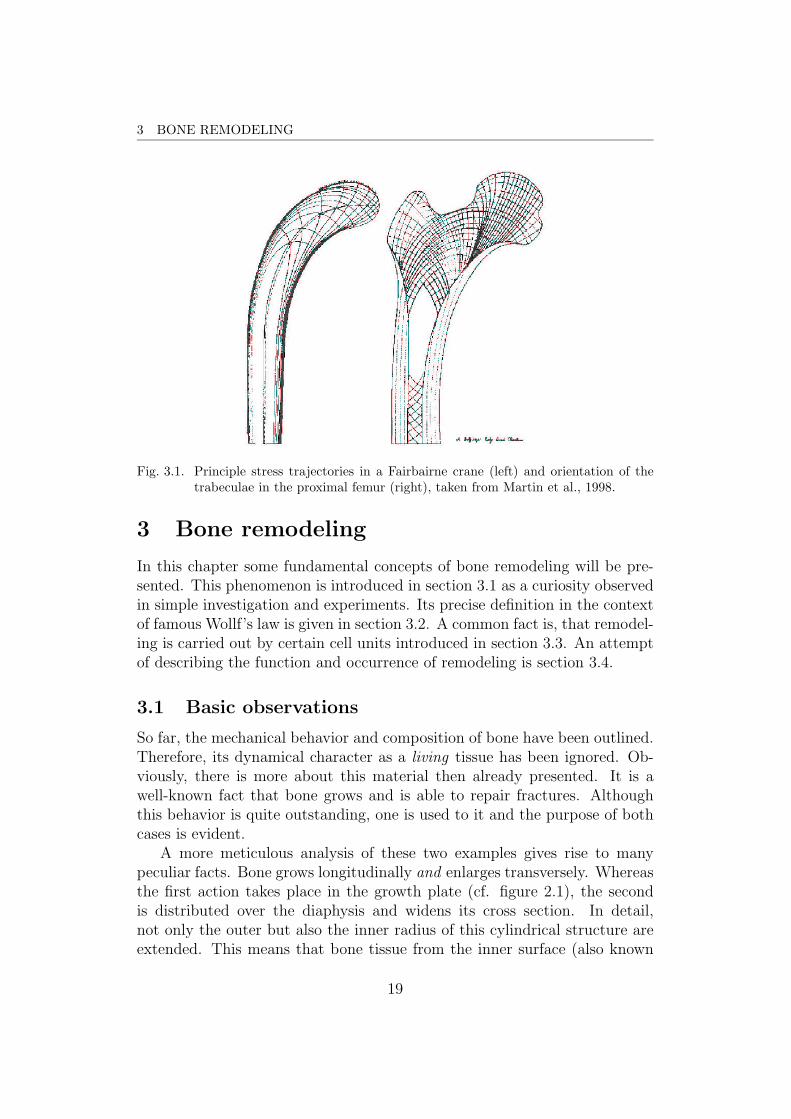
Fig. 3.1. Principle stress trajectories in a Fairbairne crane (left) and orientation of thetrabeculae in the proximal femur (right), taken from Martin et al., 1998.
3 Bone remodeling
In this chapter some fundamental concepts of bone remodeling will be pre-sented. This phenomenon is introduced in section 3.1 as a curiosity observedin simple investigation and experiments. Its precise definition in the contextof famous Wollf’s law is given in section 3.2. A common fact is, that remodel-ing is carried out by certain cell units introduced in section 3.3. An attemptof describing the function and occurrence of remodeling is section 3.4.
3.1 Basic observations
So far, the mechanical behavior and composition of bone have been outlined.Therefore, its dynamical character as a living tissue has been ignored. Ob-viously, there is more about this material then already presented. It is awell-known fact that bone grows and is able to repair fractures. Althoughthis behavior is quite outstanding, one is used to it and the purpose of bothcases is evident.
A more meticulous analysis of these two examples gives rise to manypeculiar facts. Bone grows longitudinally and enlarges transversely. Whereasthe first action takes place in the growth plate (cf. figure 2.1), the secondis distributed over the diaphysis and widens its cross section. In detail,not only the outer but also the inner radius of this cylindrical structure areextended. This means that bone tissue from the inner surface (also known
19

3 BONE REMODELING 3.1 Basic observations
as endosteum) is removed and new tissue formed on the outer surface, theperiosteum. Furthermore, the shape of each bone seems to be everythingbut arbitrary. Although never exactly the same, every bone specimen can beimmediately identified.
But the shape is not only a product of skeletal growth, since it will bepermanently maintained. In case of a fracture for example, bone is able toreconnect itself but it can also alleviate angulations, i.e., an anomalous anglebetween the connected ends resulting from a bad treatise of the fracture.
Going to a finer scale of observation, one will find the two distinct typesof bone tissue as introduced in section 2.1. Only considering long bones, thespongy trabecular bone appears in the meta- and epiphysis and the compactcortical bone in the diaphysis and as shell or cortex covering the rest ofthe bone. This way of distributing the different tissues with their differentproperties is quite impressing. In other words, it is optimal with respect tothe principle of St. Venant:† in the diaphysis with its weakly varying loadcases of bending, torsion and longitudinal forces, a dense and stiff cylindersurrounding the medullary canal is formed by the strong cortical bone tissue.On the contrary, in the ends greatly varying loads in amount and directionrequire a flexible structure for a three-dimensional state of stress providedby trabecular bone.
A classical example for this observation is represented in figure 3.1, whoseorigin was over a century ago. It shows the graphical analysis of the engineerCulmann to obtain the principle stress directions in a structure, known asFairbairne crane, next to a drawing of the mass arrangement in the proximalfemur from the anatomist von Meyer. A brief description of the pertaininganecdote can be found in Martin et al., 1998, Carter and Beaupre, 2001, orelsewhere. Any textbook on the matter will contain this story since it is aprototype of bioengineering.
The world of animal experiments provides a huge number of curious re-sults concerning bone dynamics. In Buckwalter et al., 1995, an example ispresented demonstrating the outstanding behavior of bone. Resections of thediaphysis of the ulna of pigs were realized, which impeded any load transferthrough this bone. Only after three months the cross-sectional area of theradius was almost of the size of the combined cross section of ulna and ra-dius before the interference. On the contrary, in Turner, 1999, it is shownthat metacarpals of dogs lost 60% of their original bone mass in total disuseduring 32 weeks.
Similar results can be found for the human skeleton. Vico et al., 2000,
†Due to this principle, perturbations in the region of the applied load only extend upto a distance of the size of the transversal dimension of the structure.
20

3 BONE REMODELING 3.2 Wolff’s law and the concept of remodeling
found significant reductions in bone mineral density† of weight-bearing bonesof cosmonauts which could be alleviated with reambulation. A significantalteration in the trabecular structure of the proximal femur ten years afterthe treatment of a fracture of the femoral neck with threaded pins is presentedin Buckwalter et al., 1995.
3.2 Wolff’s law and the concept of remodeling
A qualitative formulation of these observations is known under the termWolff’s law , named after the medic Julius Wolff (1836-1902). But he wasdefinitely not the first who discovered the adaptive character of bone. Asstated in Martin et al., 1998, Galilei noted the particular shape of bones asmechanical implication already in the year 1638. In 1838, Ward came up withan analogy of a streetlight bracket and the internal geometry of the femoralneck (ibidem). The anecdote of Culmann and von Meyer has been mentionedabove and took place in 1866. Indeed, there is a striking coincidence betweenthe orientation of the trabeculae and the principal stress trajectories, asshown in figure 3.1. But one has to be cautious in interpreting this incident,since the internal structure of bone is discontinuous and therefore the conceptof principle stress fails. Furthermore, the intersections of the trabecular linesare not orthogonal as principle stress trajectories have to be.
Actually, Wolff never formulated a mathematical theory and what isnowadays referred to as Wolff’s law is rather a collection of several concepts.About many of these Wolff himself did not say anything. Nevertheless, hewas one of the first, publishing ideas about adaptive processes of bone andwrote in 1892 his famous book on the subject, Das Gesetz der Transformationder Knochen.
In Martin et al., 1998, three key concepts are given as a respresentation ofthis law: the optimization of strength with respect to weight, the alignmentof trabeculae in principle stress directions, and the self-regulatory characterin response to a mechanical stimulus. The second of these ideas has beenformulated by Wolff himself. In 1872, he published the idea, that functionaladaptation reorients the trabeculae in order to align with the principal stressdirections (Cowin, 1986). An algebraic formation therefore is given in equa-tions (B.4), i.e., the coincidence of the principle axes of the fabric tensor andthe principle axes of the stress and the strain tensor, respectively, in a stateof equilibrium.
The above statements exclusively refer to the mechanical function of bone.
†Bone mineral density (BMD) is measure for the mineral content in a bone cross sectionvia x-ray absorptiometry. Cf. Hernandez, 2001, for more details.
21

3 BONE REMODELING 3.3 Basic multicellular units
But it plays an important role in the metabolism as the greatest calciumreservoir of the body. It thus serves extra-skeletal processes. In order toprovide mineral it has to be resolved from the bone matrix, carried outby osteoclasts (cf. section 2.3). On the other hand, mineral accrues fromcalcification, i.e. the formation of calcified tissue from osteoid, which itselfis formed by osteoblasts. In this sense, permanent resorption and formationtake place without influencing on shape and structure of bone.
Summarized, bone tissue underlies an ongoing change of its micro- andpossibly macrostructure. Generally, there are two denominations for thisphenomenon, modeling and remodeling . Often mixed and variously definedin literature, the declaration of Buckwalter et al., 1995, will be used here.Alterations in shape are results of modeling, whereas turnover, not influenc-ing on the shape, is termed remodeling. Widening the cross section of themedullary cavity or the age-related concavity of the vertebrae are thus ex-amples of modeling. Changes in porosity and trabeculae arrangement resultfrom remodeling. The terms external and internal remodeling are often usedto distinguish these processes. Pure modeling will be excluded from furtherconsideration, although it consists of similar cell activities. Compared to per-manent remodeling, modeling occurs rather temporarily. Furthermore, thefinal numerical analysis of modeling processes requires adaptive grids whichsimply goes beyond the scope of this work. An insight to the simulationof external remodeling by means of computer aided optimization is given inGarcıa, 1999.
3.3 Basic multicellular units
The remodeling process is carried out by certain cell units called basic multi-cellular units (BMU). A BMU consists of two cell-types, the tissue-resorbingosteoclasts and the tissue-forming osteoblasts, which have been introducedin section 2.3. The geometry of a BMU in cortical bone is cylindrical witha length of about 3mm and a width of 0.2mm and it moves at a speedof 20–40µm/day. This velocity is termed BMU-rate and will be abbrevi-ated with vBMU . It reaches a final distance of about 4mm, taking about200 days (Parfitt, 2002). A cancellous BMU has a rather irregular but elon-gated shape and measures 2–3mm in greatest dimension (Parfitt, 1994). Itsvelocity is assumed to be the half of the value for a cortical BMU. Since ittravels the same time, only half the distance will be reached. All these valuesare vague estimates and vary a lot in literature. This is not only a problemof insufficient means to determine this data but also of the dependence onthe individuals metabolism, which itself depends on age, gender, nutrition,and a variety of other factors.
22

3 BONE REMODELING 3.3 Basic multicellular units
Fig. 3.2. Schematic drawings of a cortical (a) and a cancellous (b) BMU, taken fromParfitt, 1994.
In figure 3.2 drawings of the two types of BMUs are given, clearly de-picting the order of the cell-teams. In front the multinuclear osteoclasts digthrough the tissue, followed by a zone called quiescent surface, in which nei-ther cell-type appears. Afterwards, follows the long appendage of a highnumber of osteoblasts, refilling the resorbed parts with new osteoid. Sincethis machinery needs to be nourished, it can only act on the tissue surface.This means, that in cortical bone, BMUs only exist in Haversian or Volks-mann canals or on the endo- or periosteal surfaces of the cortex. In cancellousbone, a surface position is quite evident and a BMU digs a trench.
These pictures show notably what was termed A-R-F sequence (Martinet al., 1998), representing activation, resorption, and formation. From theview of a spatially fixed observer, these processes occur in the given orderwhen a BMU passes by. Furthermore, it is obvious that a BMU is a three-dimensional object that starts at a certain point and travels in a definitedirection.
The A-R-F sequence has to be more specified. After the activation (ororigination, as will be pointed out later) a team of osteoclasts resolves thetissue matrix. This is followed by a reversal period, in which the resorptionprocess is terminated and neither cell-type appears. Afterwards, osteoblastsform the new osteoid in the formation phase.
TR, TI , and TF denote the resorption, reversal and formation period,respectively. Another quantity is the BMU lifespan, usually denoted withσ (the context will clarify the distinction between stress and lifespan). Itcould be defined as the sum of the previously mentioned time periods. Thiswould be according to a spatially fixed observer counting the time neededfor a certain BMU to pass by. On a continuum level, it is more reasonable toassign the time of activity of the osteoclasts to σ, since this measure is directlyrelated to the tissue volume, a BMU remodels. A more precise description
23

3 BONE REMODELING 3.3 Basic multicellular units
Haversiandiameter
d H
Rate ofprogression
vBMU
osteonal diameter do
BMU width dBMU
Rate ofprogression
v
Erosiondepth
d
BMU
e
Fig. 3.3. A model of the tissue volume unit a BMU resorbs of forms in cortical (left) andcancellous (right) bone tissue, adapted from Hernandez, 2001.
of this notation will be given in the context of the method developed byHernandez (Hernandez, 2001) in section 4.3.2.
The newly produced cortical bone is called osteon. It has a cylindricalshape and overlaps with other previously formed osteons thus forming themicrostructure of the tissue. The interface between the single osteons isknown as cement line and supposed to play an important role in the contextof microdamage. In Parfitt, 1994, the corresponding element for cancellousbone is termed hemi-osteon, alluding at its shape, which can be considered ahalf of an osteon. But this is a rather gross approximation, since cancellousmicrostructure is relatively irregular.
In order to analyze quantitatively the amount of resorbed and formedtissue, a geometrical model is submitted in Hernandez, 2001, clearly distin-guishing between cortical and cancellous bone. Therefore, some measureshave to be defined. In cortical bone, the diameter of a Haversian canal dHand the BMU width or osteonal diameter, do, determine together with theprogression rate, vBMU , the volume remodeled in a given time unit. With theerosion depth, de, and the BMU width, dBMU , the corresponding volume forcancellous bone can be defined. Figure 3.3 presents the shape and measuresof these volumes.
Hence, the following formulae can be given as an approach to the volumerates
Vcort =
(d2o
4− d2
H
4
)π vBMU in cortical bone (3.1a)
Vcanc =π
4de dBMU vBMU in cancellous bone. (3.1b)
The unit of these volume changes is volume per time and per BMU.
24
3 BONE REMODELING 3.4 Purpose and origination
3.4 Purpose and origination
The question why remodeling happens cannot be answered uniquely. But asusual in the context of biology, the function a certain process fulfills can besaid to be its purpose. In the following, some aspects of remodeling will bedescribed as if they were the driving forces of this phenomenon. But theymight be just side effects or eventualities.
As a repetition, the non-skeleton function as an ion reservoir has to bementioned. The contribution of bone to the metabolism mainly comes in theform of calcium. On the contrary to soft tissues, bone possesses the capacityto calcify, as already outlined. Calcium is usually provided by nutrition andits concentration therefore fluctuates. To maintain homeostasis† a permanentremodeling process is necessary for storage and retrieval of calcium.
Another aspect is the weight of bone tissue which is about the double ofsoft tissues. An overdone employment of this material would yield a muchheavier skeleton and therefore a waste of metabolic energy. Although itseems to be hardly conceivable that a global optimization can be carriedout by these microprocesses, all the above in the context of Wollf’s lawmentioned observations indicate that bone is highly optimized. Not only thesophisticated use of two different tissue types but also their distribution andorientation is striking. Additionally, bone achieves an optimal structure andis able to adapt it to environmental changes.
On the other hand, the skeleton contributes only about 6–6.5% (Martin,2003) to the overall body weight of humans whereas 52 and 40% for men andwomen, respectively, are made of muscles (ibidem). But the muscular systemitself is adaptive. A change in physical activity (be it more or less) thereforeresults in a change of bone and muscle mass with the latter being morecrucial. Increasing bone density in order to adapt to higher applied forces iscombined with an increase in body mass and so increasing the applied loadagain. This gives rise to the question whether form follows function or viceversa, extensively discussed in van der Meulen and Huiskes, 2002.
A less questionable aspect is the skeletal maintenance. A permanent re-newal of its structure prevents bone from fatigue. Although bone specimenwithstand high strain levels a significant time beyond human lifetime, dam-age repair seems to be indispensable. But fatigue life experiments are quiteabstract and cannot represent the daily loading applied in reality. This reduc-tion and the vast number of findings on damage, which vary hugely, alreadyindicate the problem. It is yet impossible to say which results are better,i.e., more realistic. Furthermore, the highly non-linear damage evolution,
†The state of equilibrium (balance between opposing pressures) in the body with respectto various functions and to the chemical compositions of the fluids and tissues.
25
3 BONE REMODELING 3.4 Purpose and origination
as pointed out in section 2.6, implies that one traumatic damage incidentreduces the predicted lifetime by many orders of magnitude. In the samecontext, imperfections influence enormously and the probability of their ap-pearance increases with increasing bone volume. Hence, the lifetime of a real,whole bone might be far below that of a specimen in a typical experiment.The removal of hypermineralized bone, i.e., bone with a very high mineral-ization degree, which is more fragile, might serve as fatigue prevention as welland simultaneously provide calcium. Despite these deliberations, it cannotbe excluded that a certain amount of remodeling is rather a stochastic thana targeted process (Parfitt, 2002).
Three characters of bone remodeling have been pointed out: the contribu-tion and storage of calcium, adaptation as a kind of structural optimization,and skeletal maintenance in the form of microdamage repair. The first ofthese functions will be waived, since it is a purely biological process. Nev-ertheless, it indicates that remodeling is a permanent process which is nottemporary due to alterations in mechanical influences.
Adaptation and damage repair shall be in the focus of this work as rel-evant processes. Since the objective is explored, the question arises howremodeling is initiated. There exists a grate amount of literature on thisquestion and a definite answer can not be given by now. In Martin et al.,1998, many approaches to this problem are presented. Signals sensed bybone cells might have their origin in stress gradients or fluid flows. Somereasonable models have been developed that are in good coincidence withexperimental data. Although the concrete way of transmission and receptionremains unknown, the existence of a certain mechanical stimulus is widelyaccepted. Different ideas will be presented in chapter 4 in the context ofmathematical descriptions on the subject.
Furthermore, the degree of damage seems to influence directly on bone re-modeling initiation. A geometrically based analysis in Martin, 2002, submitsthat a major part of or even all bone remodeling is induced by microdamage.Certainly, microcracks can destroy connections of the intercellular networkbetween osteocytes and bone-lining cells. This and other items give rise tothe concept of inhibitory signals. As outlined in Martin, 2000, a permanentstress-generated signal is emitted by these cells in order to prevent osteoclastsfrom activity. A microcrack would thus interrupt the transmission of such asignal, therefore causing activation of remodeling. Secondly, the generationof this signal could be diminished by disuse leading to more activation, too.The concept of such a signal allows for combining two effects, microdamageand disuse, which previously have been considered in a separate way.
An interesting experimental result is provided by Rubin et al., 2001. Theyshow that a high-frequency load with a very low amplitude causes an increase
26

3 BONE REMODELING 3.4 Purpose and origination
of bone density. They applied a mechanical signal causing a deformation of5×10−6 with a frequency of 30Hz to the femur of adult sheep. According tothis outcome, microdamage cannot be the only initiator of bone remodeling.Furthermore, a permanent low-level muscular activity which is omnipresent,e.g., keeping balance while standing, seems to have a significant influence onthe maintenance and adaptation of bone tissue.
The rate of initiation of a BMU was formerly described with the so-calledactivation frequency which measures the rate of penetration of a section planeby passing BMUs. It is thus a rather two-dimensional expression and lackssome precision (Hernandez et al., 1999). Since a BMU is a three-dimensionalobject, an adequate histomorphometry† takes this into account. In order todistinguish between the different concepts, the term origination frequencyis used to determine the rate of new BMUs appearing on an internal sur-face. Hernandez and co-workers have mainly developed the three-dimensionalanalysis of BMUs and their progression (Hernandez et al., 1999; Hernandez,2001).
†The quantitative measurement and characterization of microscopical images using acomputer, manual or automated digital image analysis.
27
4 COMPUTATIONAL MODELS
4 Computational models
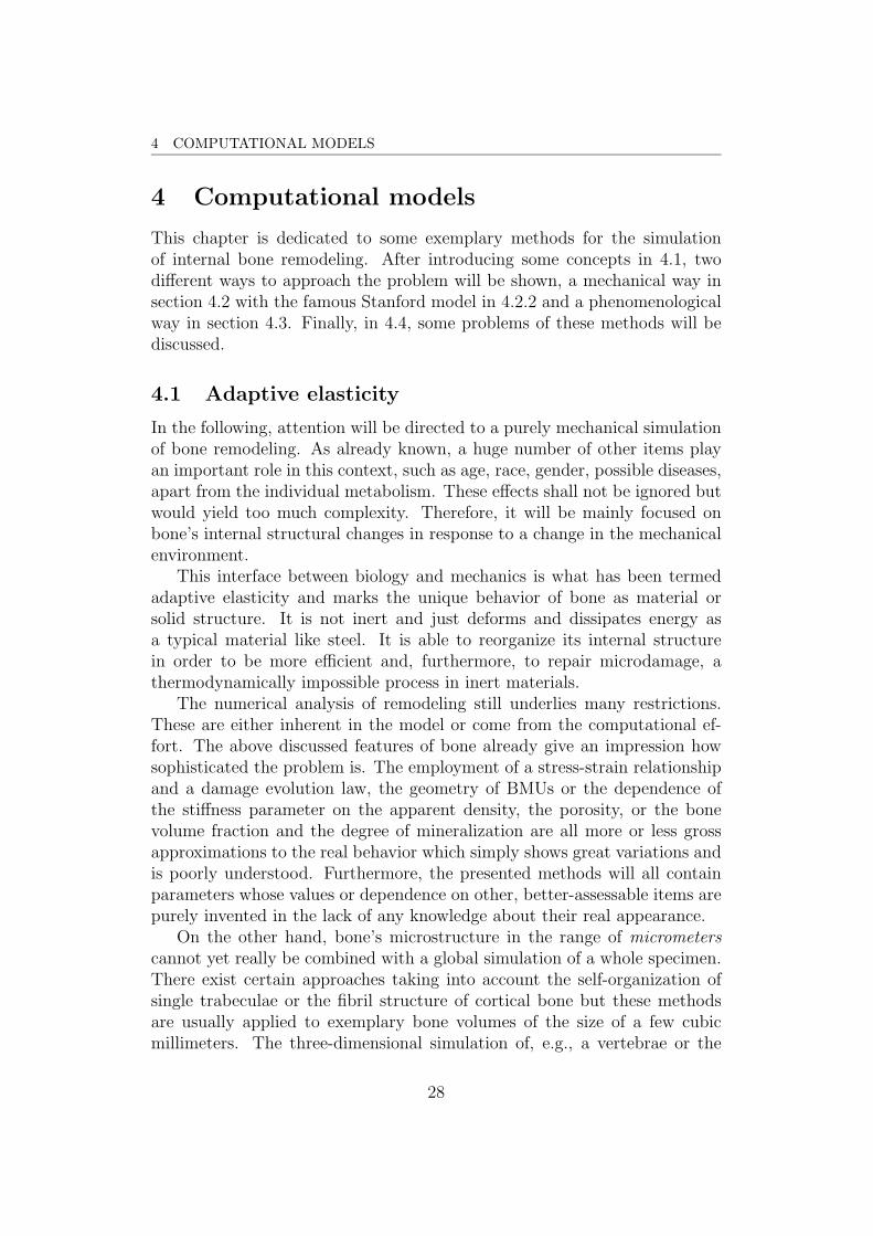
This chapter is dedicated to some exemplary methods for the simulationof internal bone remodeling. After introducing some concepts in 4.1, twodifferent ways to approach the problem will be shown, a mechanical way insection 4.2 with the famous Stanford model in 4.2.2 and a phenomenologicalway in section 4.3. Finally, in 4.4, some problems of these methods will bediscussed.
4.1 Adaptive elasticity
In the following, attention will be directed to a purely mechanical simulationof bone remodeling. As already known, a huge number of other items playan important role in this context, such as age, race, gender, possible diseases,apart from the individual metabolism. These effects shall not be ignored butwould yield too much complexity. Therefore, it will be mainly focused onbone’s internal structural changes in response to a change in the mechanicalenvironment.
This interface between biology and mechanics is what has been termedadaptive elasticity and marks the unique behavior of bone as material orsolid structure. It is not inert and just deforms and dissipates energy asa typical material like steel. It is able to reorganize its internal structurein order to be more efficient and, furthermore, to repair microdamage, athermodynamically impossible process in inert materials.
The numerical analysis of remodeling still underlies many restrictions.These are either inherent in the model or come from the computational ef-fort. The above discussed features of bone already give an impression howsophisticated the problem is. The employment of a stress-strain relationshipand a damage evolution law, the geometry of BMUs or the dependence ofthe stiffness parameter on the apparent density, the porosity, or the bonevolume fraction and the degree of mineralization are all more or less grossapproximations to the real behavior which simply shows great variations andis poorly understood. Furthermore, the presented methods will all containparameters whose values or dependence on other, better-assessable items arepurely invented in the lack of any knowledge about their real appearance.
On the other hand, bone’s microstructure in the range of micrometerscannot yet really be combined with a global simulation of a whole specimen.There exist certain approaches taking into account the self-organization ofsingle trabeculae or the fibril structure of cortical bone but these methodsare usually applied to exemplary bone volumes of the size of a few cubicmillimeters. The three-dimensional simulation of, e.g., a vertebrae or the
28

4 COMPUTATIONAL MODELS 4.2 Mechanical approach
proximal femur with consideration of the microstructure is not feasible yet.It is still a matter of computer capacity.
Although microstructural aspects are considered (especially in the BMU-based approaches of Hazelwood et al., 2001, and Hernandez, 2001), all employthe means of continuum mechanics. The basic variables will be the apparentdensity ρ, the porosity n, or the bone volume fraction VB/VT . Some conceptsemploy the degree of mineralization α or a damage measure d (or D). All ofthese variables are averaged over a certain volume V of interest (Fyhrie andSchaffler, 1995). The apparent density for example is actually defined as
ρ =1
V
∫V
ρtdV (4.1)
with ρt being the real distribution of density on the microlevel or tissuedensity as already introduced in section 2.1. Similarly, the other variablesare actually integrated values. The discussion of Fyhrie and Schaffler, 1995,on this fact results in certain restrictions on the spatial derivatives of the basicvariables which are easily violated, since the real structure of trabeculae isdiscontinuous .
Summarizing this discussion, it becomes clear that the outcome of a com-puter simulation of bone remodeling can only be of a qualitative character.The main goal is therefore to produce numerical results which show similar-ities to the experimentally observed structure. The current state of researchis still in an trial-and-error phase and postulating a quantitative precisionin the outcome is a future task.
4.2 Mechanical approach
In this section the development of algorithms for the simulation of boneremodeling from a purely mechanical point of view will be presented. Themost popular of which is the Stanford model, outlined in subsection 4.2.2with its anisotropic version in 4.2.3. In 4.2.4, a modification to the previousmodels is provided. But first, a short introduction to these concepts shall begiven.
4.2.1 History
Pauwels worked on a mathematical formulation of bone remodeling in thesixties of the last century, proposing an optimal stress level σs above whichformation and below which resorption occurs. His contemporary, Kummerdedicated his work to the self-aligning nature of bone and ran the first com-puter simulations of internal remodeling by comparing it with a second-orderfeedback system (cf. Jacobs, 1994).
29
4 COMPUTATIONAL MODELS 4.2 Mechanical approach
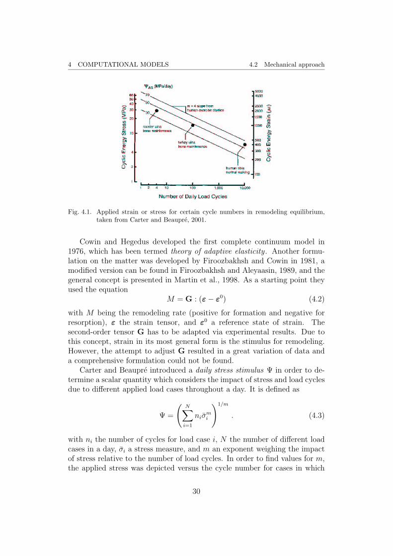
Fig. 4.1. Applied strain or stress for certain cycle numbers in remodeling equilibrium,taken from Carter and Beaupre, 2001.
Cowin and Hegedus developed the first complete continuum model in1976, which has been termed theory of adaptive elasticity . Another formu-lation on the matter was developed by Firoozbakhsh and Cowin in 1981, amodified version can be found in Firoozbakhsh and Aleyaasin, 1989, and thegeneral concept is presented in Martin et al., 1998. As a starting point theyused the equation
M = G : (ε− ε0) (4.2)
with M being the remodeling rate (positive for formation and negative forresorption), ε the strain tensor, and ε0 a reference state of strain. Thesecond-order tensor G has to be adapted via experimental results. Due tothis concept, strain in its most general form is the stimulus for remodeling.However, the attempt to adjust G resulted in a great variation of data anda comprehensive formulation could not be found.
Carter and Beaupre introduced a daily stress stimulus Ψ in order to de-termine a scalar quantity which considers the impact of stress and load cyclesdue to different applied load cases throughout a day. It is defined as
Ψ =
(N∑i=1
niσmi
)1/m
. (4.3)
with ni the number of cycles for load case i, N the number of different loadcases in a day, σi a stress measure, and m an exponent weighing the impactof stress relative to the number of load cycles. In order to find values for m,the applied stress was depicted versus the cycle number for cases in which
30

4 COMPUTATIONAL MODELS 4.2 Mechanical approach
bone mass was maintained. Such a diagram is given in figure 4.1 and thecoefficient m defines the slope of the line, since it is in logarithmic scale.m = 4 is a reasonable value which is used in most methods.
This stimulus gives rise to the Stanford model worked out in the 80’sby Carter and co-workers. In parallel, directed by Huiskes, the Nijmegenisotropic theory was developed using a quite similar approach for the stim-ulus (cf. Jacobs, 1994, for a comparison between the starting point of bothmethods). Both models have in common that they work with the apparentdensity ρ as basic variable. For some reason, the Stanford model is morefamiliar and more often cited. Therefore, it will be outlined in detail in thefollowing section.
On the contrary to soft tissues, bone is usually subjected to smalldeformations. Therefore, only a linear strain tensor will be employed
ε =12(∇⊗ u + (∇⊗ u)T
)with the gradient operator ∇ and the vector of displacements u.Furthermore, all given methods will be implemented in explicit al-gorithms, although they contain implicit formulations.
4.2.2 The isotropic Stanford model
In the following, the basic features of this famous model for the simulation ofbone remodeling will be presented. They are mainly taken from Jacobs, 1994,who analyzed its numerical stability and developed anisotropic formulation,shown in the next subsection. A gross description can be found as well inMartin et al., 1998.
First, distinction between continuum level and tissue level has to be made.Obviously, stress defined for a continuum cannot be the same as it reallyappears in the microstructure (cf. equation (4.1) for the typical averagingprocedure). Since marrow and blood vessels filling the pores are much weakerthan the calcified bone tissue, the stress, the tissue has to withstand, will beactually greater than the continuum stress. To distinguish between values ontissue and continuum level, the subscript t denotes tissue level. The relationbetween the tissue stress measure and the continuum stress measure is givenby
σ =
(ρ
ρt
)2
σt =
(VBVT
)2
σt . (4.4)
The first equality is given in Jacobs, 1994, and deduced from experimentalresults, whereas the second simply follows from the identity ρ/ρt = VB/VTas can be seen in equations (2.2) and (2.4).
31

4 COMPUTATIONAL MODELS 4.2 Mechanical approach
To define an appropriate stress measure, usually the strain energy U isemployed to represent the three-dimensional state of stress with a scalarvariable
σ =√
2EU =√Eε : C : ε (4.5)
with the Young’s modulus E and the constitutive tensor C, such that σ =C : ε.
Therefore, the above introduced stress stimulus in equation (4.3) becomes
Ψt =
(N∑i=1
niσmti
)1/m
, (4.6)
the daily tissue stress stimulus. As pointed out in figure 4.1, there exists anequilibrium stimulus, in case of which bone mass is maintained, i.e., remod-eling is in equilibrium and the apparent density (the only variable in thismodel) does not change. The condition for this equilibrium is
Ψt = Ψ∗t , (4.7)
where Ψ∗t denotes the tissue equilibrium stimulus. The deviation from thisequilibrium is assumed to be the driving force in remodeling. A stimuluserror , defined as e = Ψt−Ψ∗t , thus causes remodeling on the surface of bonetissue. Two possible forms are given as
r = c(Ψt −Ψ∗t ) , (4.8)
a simple linear relationship between the surface remodeling rate r and theerror, or as a more enhanced version
r =
c ((Ψt −Ψ∗t ) + w) for (Ψt −Ψ∗t ) < −w0 for − w ≤ (Ψt −Ψ∗t ) ≤ +w
− c ((Ψt −Ψ∗t )− w) for (Ψt −Ψ∗t ) > +w .
(4.9)
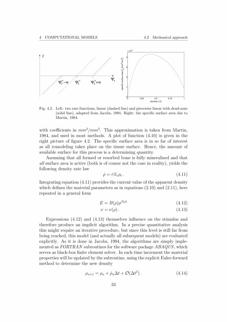
In these equations, c is a constant, which does not necessarily have to beequal for the distinct cases in (4.9). The value w denotes the half-width ofthe so-called dead zone. It is an interval around the equilibrium stimulus, inwhich no remodeling takes place. In the left picture of figure 4.2 both laws(4.8) and (4.9) are depicted.
Next, the term specific surface area (or surface density) Sv has to beintroduced. It is the internal surface area per reference volume and directlyrelated to the porosity by the polynomial
Sv = 0.02876 p5 − 0.10104 p4 + 0.13396 p3 − 0.09304 p2 + 0.03226 p (4.10)
32
4 COMPUTATIONAL MODELS 4.2 Mechanical approach
Ψ*t Ψ Ψt t
* *−w +w
r.
Ψt
0 0.25 0.5 0.75 10
1
2
3
4
x 10−3
porosity n [/]
spec
ific
surfa
ce a
rea
SA [m
m2 /m
m3 ]
Fig. 4.2. Left: two rate functions, linear (dashed line) and piecewise linear with dead-zone(solid line), adapted from Jacobs, 1994. Right: the specific surface area due toMartin, 1984.
with coefficients in mm2/mm3. This approximation is taken from Martin,1984, and used in most methods. A plot of function (4.10) is given in theright picture of figure 4.2. The specific surface area is in so far of interestas all remodeling takes place on the tissue surface. Hence, the amount ofavailable surface for this process is a determining quantity.
Assuming that all formed or resorbed bone is fully mineralized and thatall surface area is active (both is of course not the case in reality), yields thefollowing density rate law
ρ = rSvρt . (4.11)
Integrating equation (4.11) provides the current value of the apparent densitywhich defines the material parameters as in equations (2.10) and (2.11), hererepeated in a general form
E = B(ρ)ρβ(ρ) (4.12)
ν = ν(ρ) . (4.13)
Expressions (4.12) and (4.13) themselves influence on the stimulus andtherefore produce an implicit algorithm. In a precise quantitative analysisthis might require an iterative procedure, but since this level is still far frombeing reached, this model (and actually all subsequent models) are evaluatedexplicitly. As it is done in Jacobs, 1994, the algorithms are simply imple-mented as FORTRAN subroutines for the software package ABAQUS , whichserves as black-box finite element solver. In each time increment the materialproperties will be updated by the subroutine, using the explicit Euler-forwardmethod to determine the new density
ρn+1 = ρn + ρn∆t+O(∆t2) . (4.14)
33

4 COMPUTATIONAL MODELS 4.2 Mechanical approach
Although the available tissue surface Sv tends to zero when the density isvery close to the tissue density ρt, an explicit algorithm with a big time stepsize cannot prevent the outcome of a negative density, which is physically im-possible. Furthermore, it has not been observed yet that bone resorbs totally,i.e., disappears. Therefore, a lower bound ρmin will be used to compensatethis deficiency. In the same manner, an upper bound ρmax will be set in orderto impede negative porosity, i.e, a density greater than the density of a tissuewithout pores. For biological reasons, a minimal porosity (for blood supplyand nerves) has to be maintained. The expression (4.10) shall be interpretedwith caution when reaching a limit case since it predicts a non-zero amountof bone surface for 100 % porosity (cf. figure 4.2).
In the Stanford model, the isotropic material parameters En and νn andthe apparent density ρn will be passed in from time step n for every integra-tion point. After calculating the stimulus and the porosity, the remodelingrate and surface density can be evaluated, yielding the new density by meansof equation (4.14). The new density ρn+1 defines the new material parametersEn+1 and νn+1 which are passed back to the global program. In figure 4.3,a block diagram of this algorithm is presented, clearly showing its implicitstructure, and in appendix D.1 a description of an explicit version, whichwas used in the simulation, is given.
An important simplification in the calculation of the daily stimulus Ψcan be made. As outlined in Jacobs, 1994, the order of application of loadcases does not significantly affect on the computational results in a long-termanalysis. Furthermore, they can be grouped together. Taking, e.g., the threeload cases from the model of the proximal femur as introduced in appendixC, it does not really matter, whether the load cases are applied sequentiallyas in reality or reordered such that in a single day (the typical time incrementfor simulating bone remodeling) only one load case is applied. This kind ofabstraction appears to be rough but is actually negligible in relation to thereduction employed in modeling human gait. As a conclusion, equation (4.6)is simplified to
Ψt = n1/mσt , (4.15)
since only one daily load case exists.
reference stimulus: Ψ∗t = 50MPa initial density: ρ0 = 0.5 g/cm3
weighting exponent: m = 4 tissue density: ρt = 2.0 g/cm3
cycles per day: n = 10, 000 minimal density: ρmin = 0.05 ρtremodeling velocity: c = 0.02 maximal density: ρmax = 0.95 ρthalf-width of dead zone: w = 0.125 Ψ∗t time step size: ∆t = 1 day
Tab. 4.1. Values used for the parameters in the simulation with the Stanford model
34

4 COMPUTATIONAL MODELS 4.2 Mechanical approach
global FEM-Analysis
?U
σ =√
2EU
?σ
Ψ = n1/mσ
?Ψ
Ψt = (ρtρ
)2Ψ -Ψt e = Ψt −Ψ∗t -e
r
e
?
Ψ∗t
-
6
Sv
ρ-
6 ρ = rSvρt
∫-ρ-Sv -ρ
-ρ
-ρ?r
E = B(ρ)ρβ(ρ)
ν = ν(ρ)ρ
new Materialparameters
Local integrationpoint level
Fig. 4.3. A block diagram of the algorithm of the isotropic Stanford model.
The presented algorithm of the Stanford isotropic model is applied in theabove described manner to the two-dimensional model of a proximal femur inhuman gait. This model exhibits some interesting properties of the method,although it cannot be identified as a realistic case.
The values in table 4.1 are assigned to the above introduced parametersof this model. In figure 4.4, results for the apparent density after 100, 300,500, 1000, 3000, and 4000 days are shown for the standard time step sizeof 1 day. For comparison, a radiograph of the proximal femur is presented,too. The best concordance can be seen in the result after 300 days. Itcontains the basic structural elements, like the cortex, medullary canal, andthe qualitative distribution of the trabecular density. Unfortunately, theresults become worse, as time passes by and the predicted structure is after4000 days much less coincident with reality. Furthermore, discontinuitiesarise, which are mesh dependent, as outlined in Mullender et al., 1994, andZhu et al., 2002. Jacobs himself analyzed the instability of this method andproposed quadratic elements or nodal presentation of the values rather thanin the integration points (Jacobs, 1994). These means alleviate the problemof discontinuities, but the method itself remains unstable. A convergence
35

4 COMPUTATIONAL MODELS 4.2 Mechanical approach
Fig. 4.4. From left to right, results of a simulation with the Stanford isotropic model forthe distribution of the apparent density ρ after 100, 300, and 500 days in the toprow and after 1000, 2000, and 3000 days in the middle row. In the bottom row,the result after 4000 days and radiograph of the proximal femur, from Garcıa,1999, are given. The legend assigns numerical values of ρ in g/cm3 to the usedcolor scale.
36

4 COMPUTATIONAL MODELS 4.2 Mechanical approach
Fig. 4.5. Plot of the convergence parameter δ, which presents an averaged density change,for the first 4000 days. In the upper right corner, a zoom of the result for thedays 3000–4000 is given, clearly showing the oscillatory behavior.
analysis indicates this weakness. Note that convergence is meant in the sense,that the numerical results tends in a stable way to a solution, consistency isnot proved. Therefore, a parameter
ζ =
∫V|ρ|dV∫VdV
(4.16)
was used, which gives an average of the density change for the volume ofthe whole model. As it can be seen in figure 4.5, this parameter decreasesrapidly but does not reach 0. Even after 4000 days (approximately 11 years),convergence is not reached. On the contrary, the value of ζ oscillates around2× 10−4 g/(cm3day) with an amplitude of approximately 1.5× 10⁻⁴.
Hence, it can be stated that the presented model is not stable. In themeantime, it produces creditable results but they disappear in a long-termsimulation. The question whether a stable remodeling equilibrium exists, hasnot been answered yet, but due to the assumptions of the method, such astable solution should exist. Nevertheless, the simulation does not come upwith a convergent tendency. Apart from these results, one shall doubt whatthe model of the proximal femur can predict. This will be discussed later onin the context of a new formulation.
4.2.3 Anisotropic extension
In the work of Jacobs (Jacobs, 1994), two ways are shown to extend theabove presented isotropic method to anisotropy. He derives an energy-based
37

4 COMPUTATIONAL MODELS 4.2 Mechanical approach
and a stress-based formulation, whereas the former will be shown here.The stress-strain relationship
σ = C : ε
is no longer necessarily isotropic and cannot be represented by the two pa-rameters E and ν only. The idea of Jacob is to find an evolution law for thematerial tensor C, i.e., a rule for its temporal derivative, C.
The starting point for this derivation is the postulate that bone remod-eling be optimal in an energetic sense. Applying the standard means ofcontinuum mechanics: bone occupies a region Ω with closed boundary Γ.The external mechanical power can then be expressed as
Pe =
∫Γ
t · vdΓ +
∫Ω
b · vdΩ (4.17)
with the traction vector t, the body forces b, and the velocity field v,where the latter includes elastic deformation as well as the adaptive response.Therefore, atrophy corresponds to Pe > 0 and hypertrophy to Pe < 0, whichin terms of mechanics denote a loss or an increase of stiffness, respectively.Since applied body forces are of a negligible magnitude compared to the ap-plied traction, the second term in equation (4.17) can be set to zero. Theefficiency of the adaptive process can be measured with the mechanical dis-sipation E defined as
E = Pe −d
dt
∫Ω
χ+KdΩ , (4.18)
where χ is the internal energy density and K the kinetic energy density,K = 1
2|v|2ρ.
The total energy dissipation will be
D = E + B , (4.19)
which is the sum of the mechanical and the biological dissipation. In inertmaterials, the latter does not exist and, therefore, the thermodynamic re-striction, that the energy dissipation has to be non-negative, applies directlyon the mechanical part E . In the given case, a certain magnitude of biologicalenergy dissipates which cannot be quantified by no means. Without violat-ing the thermodynamic laws, E can be negative with D still being positive.This is the particularity of living tissues: mechanical energy can be gained(and damage can be repaired). Taking the mechanical energy balance equa-tion (Ogden, 1984), the external power equals the sum of the rate of change
38

4 COMPUTATIONAL MODELS 4.2 Mechanical approach
of the kinetic energy and the rate of work of stresses (stress power)
Pe =d
dt
∫Ω
1
2|v|2ρdΩ +
∫Ω
σ : εdΩ .
Inserting this result into equation (4.18), yields a more convenient expressionfor the mechanical energy dissipation
E =
∫Ω
σ : ε− χdΩ , (4.20)
which is the difference between the stress power and change in internal po-tential energy.
In case of a purely elastic deformation, quantity (4.20) would be identi-cally zero. In inert materials, it would have the restriction to be non-negative,but here it can be negative due to metabolic forces.
Moreover, an assumption on the internal energy density χ will be madein such a form that it depends on the strain, the stiffness tensor and theapparent density
χ(ε,C, ρ) =1
2ε : C : ε+ Θ(ρ) (4.21)
where Θ(ρ) is functional dependence of the internal energy density on theapparent density changes. The presumed optimality of the adaptive responsecomes now in terms of C provoking an extreme value of mechanical dissipa-tion E . Differentiating (4.21) with respect to time and inserting the resultinto (4.20) yields
E =
∫Ω
−1
2ε : C : ε−Θ′ρ dΩ . (4.22)
Since the remodeling process is restricted, its side conditions have to be for-mulated. As in the isotropic case, the deviation of the stimulus from a refer-ence stimulus causes resorption or formation. The mathematical expressionis
f j(ε,C, ρ) ≤ 0 (4.23)
with the superscript j referring to formation or resorption. These conditionsare derived from equation (4.9) and are explicitly
f f = n1/mρ2t
√B√ε : C : ε− (Ψ∗t + w)ρ2−β/2 ≤ 0
f r = −n1/mρ2t
√B√ε : C : ε+ (Ψ∗t − w)ρ2−β/2 ≤ 0
for formation and resorption, respectively. The parameters are all identicalwith those introduced in the isotropic method. These expressions have now
39

4 COMPUTATIONAL MODELS 4.2 Mechanical approach
the form of a yield-criterion in the theory of plasticity and the Langrangeancan be formulated
L = −E +∑j
[∫Ω
γjf j(ε,C, ρ)dΩ
],
where γj are the Langrange multipliers for each criterion. Requiring that thefirst variation δL = 0, leads finally to the expression∫
Ω
(∑j
(γj∂f j
∂ε
)+ C : ε
): δε+
(∑j
(γj∂f j
∂ρ
)+ Θ′′ρ
): δρ dΩ = 0 .
(4.24)Since δε and δρ can be chosen arbitrarily under certain conditions, the corre-sponding terms in equation (4.24) have to vanish. The optimality conditionsare therefore
C : ε = −∑j
(γj∂f j
∂ε
)and Θ′′ρ = −
∑j
(γj∂f j
∂ρ
)(4.25)
and the Kuhn-Tucker conditions
γj ≥ 0 , f j ≤ 0 and γjf j = 0 . (4.26)
Splitting the criteria into a part corresponding to the strain and a part cor-responding to the density
f j(ε,C, ρ) = Φj(ε,C)−Rj(ρ)
and using the homogeneity of degree one in ε of the terms Φj, provides aftersome manipulation the rate of change law of the material tensor
C =∑j
(γj
Φj
∂Φj
∂ε⊗ ∂Φj
∂ε
).
This symmetric, positive-definite form can be adjusted with equation (4.23),yielding the final form of the stiffness evolution
C =βρ
ρ
σ ⊗ σσ : ε
. (4.27)
Actually, the density ρ underlies the same evolution law as in the isotropiccase, but now reformulated with the criteria (4.23)
ρ =
− cf
r(ε,C, ρ)
ρ2−β/2 Sv(ρ) if f r ≥ 0, f f < 0
0 if f r < 0, f f < 0
cf f (ε,C, ρ)
ρ2−β/2 Sv(ρ) if f r < 0, f f ≥ 0
, (4.28)
40
4 COMPUTATIONAL MODELS 4.2 Mechanical approach
where Sv is the tissue surface in dependence on the porosity (and thereforedensity) as introduced in (4.10).
Now, the basic steps of the algorithm can be given in incremental form
ρn+1 = ρn + ρn∆t+O(∆t2) (4.29a)
Cn+1 = Cn + Cn∆t+O(∆t2) . (4.29b)
An explicit algorithm can thus be easily formulated, updating the basic vari-ables ρ and C in each integration point for every time step. Due to a possibleloss of positive definiteness in the resorption case, ρ < 0, numerical problemscan occur (cf. Jacobs, 1994). They can be omitted by updating the com-pliance tensor F = C−1 and inverting it back to the stiffness tensor in thiscase. The rate of change for the compliance tensor is derived by means ofF = −F : C : F to the form
F =βρ
ρ
ε⊗ εσ : ε
. (4.30)
A summary of this algorithm will be given in the appendix D.2.With this anisotropic extension of the Stanford model the same example
of the proximal femur was analyzed. The density distribution is similar tothe isotropic model. The degree and principal directions of anisotropy ofthe stiffness tensor C was depicted on the left side of figure 4.6, which ispresented at the end of the next subsection for a better comparison with thefollowing method. The used parameters are identical to the isotropic caseand given in table 4.1.
4.2.4 Enhancement proposed by Garcıa and Doblare
Jacob proposed two independent variables in his anisotropic extension of theStanford model, the apparent density ρ and the stiffness tensor C, whoseevolution is the basis of his method (Jacobs, 1994). But actually, thesevariables are not independent. They are coupled as can be seen in equation(4.27), where it is shown that the evolution of the stiffness tensor dependsdirectly on the density rate of change.
Furthermore, there is no statement, whether the mechanical energy dis-sipation (or efficiency) assumes its minimum or maximum due to the remod-eling process. In standard plasticity of inert materials, an associated plasticstrain evolution is used which means that the maximal energy is dissipated.
Another problem is the outcome of this method which is far away fromreality. The degree of anisotropy resulting in the proximal femur model andshown in figure 4.6 is much too high as discussed later.
41
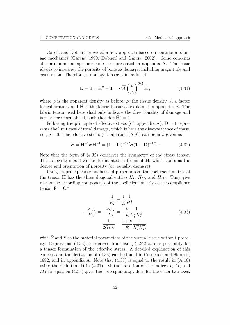
4 COMPUTATIONAL MODELS 4.2 Mechanical approach
Garcıa and Doblare provided a new approach based on continuum dam-age mechanics (Garcıa, 1999; Doblare and Garcıa, 2002). Some conceptsof continuum damage mechanics are presented in appendix A. The basicidea is to interpret the porosity of bone as damage, including magnitude andorientation. Therefore, a damage tensor is introduced
D = 1−H2 = 1−√A
(ρ
ρt
)β/2H , (4.31)
where ρ is the apparent density as before, ρt the tissue density, A a factorfor calibration, and H is the fabric tensor as explained in appendix B. Thefabric tensor used here shall only indicate the directionality of damage andis therefore normalized, such that det(H) = 1.
Following the principle of effective stress (cf. appendix A), D = 1 repre-sents the limit case of total damage, which is here the disappearance of mass,i.e., ρ = 0. The effective stress (cf. equation (A.8)) can be now given as
σ = H−1σH−1 = (1−D)−1/2σ(1−D)−1/2 . (4.32)
Note that the form of (4.32) conserves the symmetry of the stress tensor.The following model will be formulated in terms of H, which contains thedegree and orientation of porosity (or, equally, damage).
Using its principle axes as basis of presentation, the coefficient matrix ofthe tensor H has the three diagonal entries HI , HII , and HIII . They giverise to the according components of the coefficient matrix of the compliancetensor F = C−1
1
EI=
1
E
1
H4I
−νI IIEII
= −νII IEI
= − νE
1
H2IH
2II
1
2GI II
=1 + ν
E
1
H2IH
2II
(4.33)
with E and ν as the material parameters of the virtual tissue without poros-ity. Expressions (4.33) are derived from using (4.32) as one possibility fora tensor formulation of the effective stress. A detailed explanation of thisconcept and the derivation of (4.33) can be found in Cordebois and Sidoroff,1982, and in appendix A. Note that (4.33) is equal to the result in (A.10)using the definition D in (4.31). Mutual rotation of the indices I, II, andIII in equation (4.33) gives the corresponding values for the other two axes.
42

4 COMPUTATIONAL MODELS 4.2 Mechanical approach
Since the basis of this presented method is the isotropic Stanford model,the above used material properties are
E = B(ρt)ρβ(ρt)t = 1763 ρ3.2
t and ν = ν(ρt) = 0.32 . (4.34)
The mechanical stimulus shall now be the associate variable to the re-modeling tensor H in the free energy function ψ = 1
2ε : C : ε as defined in
appendix A
YH =∂ψ(ε,H)
∂H=∂ψ
∂σ
∂σ
∂H, (4.35)
which will be denoted for convenience with Y instead of YH. This variablecan be represented as (cf. Garcıa, 1999, for details on this and followingderivations)
Y = 2(λ tr(H2ε)Hε+ 2µ(HεH)(Hε)
)(4.36)
with the Lame parameters according “the undamaged” parameters E and ν
λ =Eν
(1 + ν)(1− 2ν)and µ =
E
2(1 + ν).
Actually, equation (4.36) is stated with symmetrized tensor expressions. Butthis is redundant since a linear strain tensor is employed and the fabric tensoris symmetric by definition (cf. equation (B.3) and subsequent explanation inappendix B).
It can be shown that the complementary stimulus Yσ, taking the stressas independent variable and the complementary energy ψ∗ as starting point,is the negative of the above defined stimulus, Yσ = −Y.
In order to analyze the impact of isotropic and anisotropic components,respectively, a tensor function J is introduced
J =1
3(1− ω) tr(Y)1 + ω dev(Y) =
1
3(1− 2ω) tr(Y)1 + ωY (4.37)
which weighs the spherical and deviatory parts of the stimulus with a pa-rameter ωε[0, 1]. In this sense, ω = 0 corresponds to an isotropic and ω = 1to a maximally anisotropic case.
In consistency with a yield or damage criterion, the dead zone of remod-
43

4 COMPUTATIONAL MODELS 4.2 Mechanical approach
eling will be now delimited by the following criteria
gr =
√2(1− ω)
n1/m√BA1/8271/4ρ
2−β/8t
(J−1 : J−1
)1/4 − 1
(Ψ∗t − w)ρ(16−5β)/8< 0
(4.38a)
gf =n1/m√BA1/831/4ρ
2−β/8t√
2(1− ω)(J : J)1/4 −(Ψ∗t + w)ρ(16−5β)/8 < 0
(4.38b)
The next step is to find an evolution law for the remodeling tensor H.This will be proposed according to a plastic strain evolution with an associatelaw
H = µr∂gr
∂Y+ µf
∂gf
∂Y,
where the following conditions have to be fulfilled
µr , µf ≥ 0 , gr , gf ≤ 0 , and µrgr = µfgf = 0 .
In order to determine the proportionality factors µj, consistency of the isotropiccase with the Stanford model is postulated yielding the expressions
H =
3βkrSv
4 tr(H−2J−3 : ωH)
ρtρ
J−3 : ω in resorption
3βkrSv4 tr(H−2J : ωH)
ρtρ
J : ω in formation,
(4.39)
where a new tensor ω has been introduced, defined as
ω =1
3(1− 2ω))1⊗ 1 + ωI (4.40)
with the second-order unit tensor 1 and the fourth-order unit tensor I. Ev-idently, H = 0 if neither resorption nor formation occurs. Note that inequation (4.39) a factor k is introduced which tunes the fraction of availablebone surface which is active. All the remaining parameters are previouslyintroduced or equivalent to the Stanford isotropic model and the surfaceremodeling rate obeys the same rule as expressed in equation (4.9).
Knowing the value of the remodeling tensor H, the current density canbe determined by means of the determinant of H using its definition (4.31)
ρ = ρt
(det H2
A3/2
)2/(3β)
. (4.41)
44

4 COMPUTATIONAL MODELS 4.2 Mechanical approach
Fig. 4.6. Directionality and magnitude of stiffness for the proximal femur as predictedby the method of Jacobs, 1994, on the left side, by the method of Garcıa andDoblare (Garcıa, 1999;Doblare and Garcıa, 2002).
Employing again the explicit Euler-forward method, allows for the inte-gration of equations (4.39) in order to obtain the new remodeling tensor
Hn+1 = Hn + ∆tHn +O(∆t2) (4.42)
which will be then used to determine the current stiffness tensor Cn+1 bymeans of expressions (4.33), coordinate transformation and inversion of thecompliance tensor Fn+1.
A summary of this algorithm will be given in appendix D.3. Results ofa computer simulation are given in Garcıa, 1999, and Doblare and Garcıa,2002. It was applied to the proximal femur model (cf. appendix C) usingthe same parameters as in the isotropic Stanford model as given in table 4.1.The newly introduced parameter k was set to 1.0 in order to compare theresults with those presented in Jacobs, 1994. The density distribution is notpresented here, since it is similar to the isotropic model (cf. figure 4.4).
In figure 4.6, the stiffness with magnitude and directionality after 300 daysis given for the anisotropic extension of the Stanford model (left picture) andfor the new model of Garcıa and Doblare (right picture). One can observethat the predicted degree of anisotropy is excessively high in the model ofJacobs. Furthermore, the magnitude is much below realistic values. A sig-
45
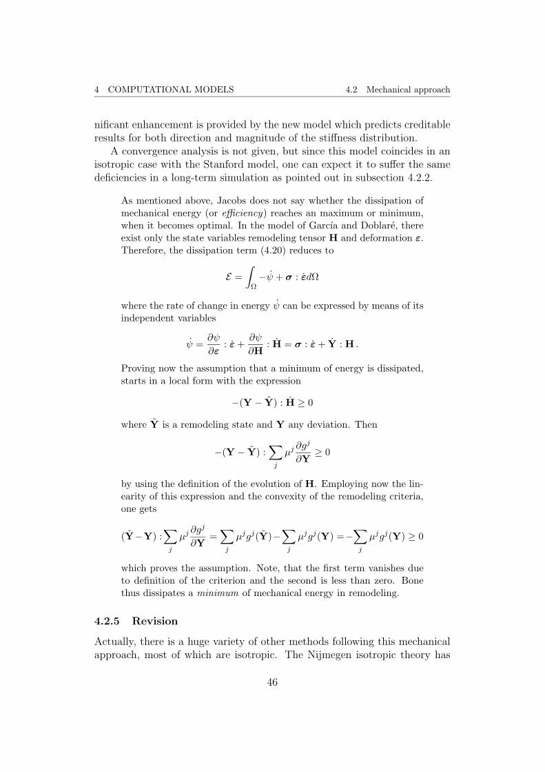
4 COMPUTATIONAL MODELS 4.2 Mechanical approach
nificant enhancement is provided by the new model which predicts creditableresults for both direction and magnitude of the stiffness distribution.
A convergence analysis is not given, but since this model coincides in anisotropic case with the Stanford model, one can expect it to suffer the samedeficiencies in a long-term simulation as pointed out in subsection 4.2.2.
As mentioned above, Jacobs does not say whether the dissipation ofmechanical energy (or efficiency) reaches an maximum or minimum,when it becomes optimal. In the model of Garcıa and Doblare, thereexist only the state variables remodeling tensor H and deformation ε.Therefore, the dissipation term (4.20) reduces to
E =∫
Ω−ψ + σ : εdΩ
where the rate of change in energy ψ can be expressed by means of itsindependent variables
ψ =∂ψ
∂ε: ε+
∂ψ
∂H: H = σ : ε+ Y : H .
Proving now the assumption that a minimum of energy is dissipated,starts in a local form with the expression
−(Y − Y) : H ≥ 0
where Y is a remodeling state and Y any deviation. Then
−(Y − Y) :∑j
µj∂gj
∂Y≥ 0
by using the definition of the evolution of H. Employing now the lin-earity of this expression and the convexity of the remodeling criteria,one gets
(Y−Y) :∑j
µj∂gj
∂Y=∑j
µjgj(Y)−∑j
µjgj(Y) =−∑j
µjgj(Y) ≥ 0
which proves the assumption. Note, that the first term vanishes dueto definition of the criterion and the second is less than zero. Bonethus dissipates a minimum of mechanical energy in remodeling.
4.2.5 Revision
Actually, there is a huge variety of other methods following this mechanicalapproach, most of which are isotropic. The Nijmegen isotropic theory has
46

4 COMPUTATIONAL MODELS 4.3 Phenomenological approach
already been mentioned, which provides an alternative to the Stanford model.Similarly, many other methods can be compared to these famous models inthat sense that they have the same basis: the apparent density evolves intime as a direct response to a certain mechanical stimulus.
In Stulpner et al., 1997, a different stimulus is proposed which is strain-based and a different law for remodeling rate r is used. The latter modifica-tion surely implies an enhancement because the law employed in the Stanfordmodel is not limited, i.e., a very high or low stimulus causes excessive remod-eling rates. This is physically not meaningful and the asymptotic behaviorof a double-sigmoid, as assumed here, appears to be more reasonable.
In fact, the Stanford model can theoretically lead to negative densitiesdue to its quasi-linear evolution law. This is impeded by forcing the solutionto stay within certain limits. An improvement is provided by Fyhrie andSchaffler, 1995, who propose a model based on an exponential law fit toexperimental data for disuse. Unfortunately, its benefit is restricted to thatcase of disuse and useful results concerning formation of bone could not beproduced (Garcıa, 1999).
A mathematically very advanced theory is given by Ramtani and Zidi,2001. This model is based on continuum thermodynamics and formulated ina very general way. Being derived from momentum and energy balance laws,it provides the necessary restrictions on damage evolution. Furthermore, asmall-strain version is presented, too. Nevertheless, this model has not beenimplemented numerically and therefore lacks some verification.
To circumvent the numerical instabilities in the Stanford model, Mullen-der et al., 1994, propose an approach in which sensor cells with a certainrange of sensitivity are attached to the FE-model independent of the appliedmesh. These cells sense the mechanical stimulus and activate remodeling.This procedure is rather applicable to the microstructure, when the elementsize is smaller than the range of sensitivity. But on this scale the standardmeans of continuum mechanics do not apply anymore and the predicted re-sults are doubtful (Fyhrie and Schaffler, 1995).
4.3 Phenomenological approach
All the above presented models have in common, that they do not considerthe mechanisms taking place internally in bone tissue. Neither the geome-try of a remodeling cell unit (BMU), the time consumption of the differentstages of the remodeling process, nor the inherent coupling of formation andresorption are taken into account. In the following, two BMU-based conceptswill be presented which appeared in the given order in literature.
47

4 COMPUTATIONAL MODELS 4.3 Phenomenological approach
4.3.1 The method of Hazelwood, Martin et al.
The model provided by Hazelwood et al., 2001, was unique when presentedfor the first time. It considers the full A-R-F sequence of a BMU, as intro-duced in section 3.3, i.e., the fact that an activated BMU always starts withresorption before it forms new tissue. Furthermore, the rate of activation,progression velocity, and dimensions of a BMU are regarded. But this modelis purely two-dimensional.
The basic equation of this model is the rate of change of porosity
p = QRNR −QFNF (4.43)
which is given in terms of the density of resorbing and forming BMUs, NR
and NF , respectively, given in the unit BMUs/area. The factors QR and QF
describe the volume rates for resorption and formation, respectively. Theyare assumed to be linear in time and given by QR = A/TR and QF = A/TF ,where A denotes the cross-sectional area of a BMU (determined by the crosssection of an osteon, cf. section 3.3), TR the resorption period, and TF theformation period. Note that (4.43) is formulated in terms of the porosity pand not as in the previous method with the density ρ. But both are easilyrelated by p = 1− ρ/ρt.
Another restriction of this method is, that all the values are assumedfor cortical bone. Therefore, the volume rates QR and QF are constant (cf.section 3.3 for the distinction between osteonal and hemi-osteonal volumes asintroduced by Parfitt, 2002, and applied in Hernandez, 2001). The dynamicsof bone are thus regulated by the number of BMUs in each of the possibleremodeling states. They are given in terms of the activation frequency fa as
NR =
∫ t
t−TRfa(t
′)dt′ (4.44a)
NF =
∫ t−TR−TI
t−TR−TI−T−Ffa(t
′)dt′ . (4.44b)
Recall that TI denotes the reversal period in which a BMU turns over fromresorption to formation. How a BMU progresses, can be seen from equations(4.44): at a fixed point in space it passes by, needing TR for resorption, TIto change, and TF to form. So, at a given point in time one can state thatthose BMUs are forming, which were activated more than TR + TI ago, andthose are resorbing, which were activated recently, not longer than TR ago.This concept is coinciding with experimental observations due to which boneremodeling (internal remodeling, neither external remodeling nor growth) is
48

4 COMPUTATIONAL MODELS 4.3 Phenomenological approach
always carried out by coupling osteoclasts and osteoblasts and thus alwaysstarting with resorption.
The two-dimensional term activation frequency, fa, describes the numbersof BMUs appearing in a given cross section in a certain time interval. In thismodel, the main items of remodeling are adaptation in disuse (as a kindof weight optimization) and damage removal. The activation frequency istherefore determined by the two parts
fa = Sv(fa,dis + fa,dam) , (4.45)
where fa,dis and fa,dam refer to activation due to disuse and damage, respec-tively. Another driving factor is the available surface area, since remodelingtakes only place on internal tissue surfaces. Therefore, the term Sv is usedwhich the same as used in the previous methods (cf. Sv in equation (4.10)and figure 4.2), but normalized to the interval [0, 1].
Before giving the expressions for the activation frequency, the applieddamage law and mechanical stimulus have to be introduced. Damage shallevolve due to
D = DM − DR (4.46)
with a damage increase DM caused by mechanical impact and damage de-crease DR caused by remodeling. The former is a function of the appliedstimulus Φ
DM = kDΦ = kD∑i
εqiNi (4.47)
and the latter is a function of the damage state and the activation frequency
DR = DfaAFs . (4.48)
In these expressions, kD denotes the damage rate coefficient given by kD =D0fa,0AFs/Φ0 with the initial damage state D0, the initial activation fre-quency fa,0, the BMU cross section A, the damage removal factor Fs, andthe initial mechanical stimulus Φ0. Furthermore, ε is a strain measure, q aweighting exponent, and N the number of cycles, with the index i indicatingthe load cases. Note, that in this approach damage is not the continuumdamage as introduced in appendix A but measuring the crack length persurface area. It can therefore not be identified with the typical damage vari-able varying between 0 and 1. Moreover, the employed strain measure wasassumed to be the principle compressive strain. This choice has not beenfurther elaborated, it is just a possibility out of many.
Another simplification of this model is that the same stimulus Φ is usedfor damage evolution and disuse activation. As pointed out by the authors,
49

4 COMPUTATIONAL MODELS 4.3 Phenomenological approach
0 0.5 1 1.5 0
0.25
0.5
stimulus Φ [10−10cpd]
f a,di
s [BM
Us/
mm
2 /day
s]
Φ0 0 0.25 0.5
0
0.25
0.5
damage D [mm/mm2]
f a,da
m [B
MU
s/m
m2 /d
ay]
D0
Fig. 4.7. Plots of the functions describing the activation frequency fa. Right: remodelingactivated by disuse, cf. equation (4.49). Left: activation through by damage asin equation (4.50). The parameters have the values as in table 4.2.
this has been done for convenience and not in the assumption that damageis driven by the same force as remodeling due to disuse.
Nevertheless, if the disuse criterion Φ < Φ0 is fulfilled, remodeling isactivated by
fa,dis =fa,max
1 + ekb(Φ−kc)(4.49)
with kb and kc coefficients that define the shape of this function and fa,maxthe maximal possible activation frequency. In a similar manner, damageactivates remodeling in the form of
fa,dam =fa,0fa,max
fa,0 + (fa,max − fa,0)ekrfa,max(D−D0)/D0(4.50)
with another factor kr. The curves of the activation frequency in functionof disuse or damage are given in figure 4.7. In case of disuse, the crosssection for the formation rate QF = A/TF is replaced by a reduced valueA = A(0.5 + 0.5 Φ/Φ0) in order to consider reduced formation in disuse.
The new porosity pn+1 at time instant tn+1 can be determined in thestandard explicit way
pn+1 = pn + p∆t+O(∆t2) (4.51)
with p due to equation (4.43).The only used material parameter in this context is the Young’s modulus
as already introduced in equation (2.12) and repeated here for completeness
E = E(p) = 8.83× 10² p6 − 2.99× 10³ p5 + 3.99× 10³ p4
− 2.64× 10³ p3 + 9.08× 10² p2 − 1.68× 10² p+ 23.7 (4.52)
50

4 COMPUTATIONAL MODELS 4.3 Phenomenological approach
global FEM-Analysis
?
Φ =∑
i εqNi
?
DM = kDΦ
DR = DfaAFs
?
6
D?
6
fa,dam(D) fa,dis(Φ)?
Φ < Φ0
fa = SV (fdam + fa,dis)
6? ?
NR =∫fa
NF =∫fa
6
n = QRNR−QFNF
6
nE(n)
6
new Materialparameters
Local integrationpoint level
Fig. 4.8. A block diagram of the algorithm for the method of Hazelwood et al. Thedependence of the specific surface area Sv on the porosity n and the dependenceof the strain measure ε on the current Young’s modulus E have not been depictedfor sake of simplicity. Functional expressions are given in the text. Furthermore,the formation rate is calculated with a reduced surface area A in case of disuse.
with units of GPa.With these equations the model is fully defined and can be implemented
numerically. The used parameters are summarized in table 4.2 together withthe values they assume. A visualization of the algorithm in its fully implicitform is given in figure 4.8 and its explicit form will be summarized in appendixD.4.
The algorithm was tested in order to reproduce the published results. Inthe same manner as the Stanford model, it was implemented as a user sub-routine to the ABAQUS -package. The time step-size was set to the standardvalue of ∆t = 1 day. Since this method depends on the history as clearlystated in the integral expressions (4.44), global arrays storing the past acti-vation frequencies for a period of TR+TI +TF have been employed. The testmodel has been a quadratic cross section with an area of 100mm2. It wassupported and loaded symmetrically and the Poisson ratio was set to ν = 0,since it has not been mentioned. The initial porosity was set to p0 = 0.0443,a typical value for cortical bone. Therefore, the initial Young’s modulus wasE0 = 17.8GPa. Using the parameters of table 4.2, a compressive force of891.6N yielded directly equilibrium without any change in porosity.
In figure 4.9, the porosity evolution for applied forces of 445.8, 891.6,
51

4 COMPUTATIONAL MODELS 4.3 Phenomenological approach
0 500 1000 1500 20000
0.1
0.2
0.3
0.4
time [days]
poro
sity
n [/
]
445 kN 892 kN1640 kN1655 kN
Fig. 4.9. Evolution of the porosity for different applied loads for the first 2000 days. Theinitial porosity is p0 = 0.0443.
1640, and 1655N magnitude is presented. Simulation was run for 2000 daysand exhibited convergence except for the case of 1655N . Here, the damagegrowth is faster than its removal due to remodeling. It can be observed thatin either cases of deviation from equilibrium resorption takes place. Althoughformation is restricted due to the low initial porosity, one might expect theporosity to be maintained in the case of overload. But overload activates viadamage and any activation causes initially resorption. Therefore, startingwith a higher initial porosity and the same initial activation frequency would
cross section of a BMU: A = 2.84× 10⁻²mm2
resorption period: TR = 24 daysreversal period: TI = 8 daysformation period: TF = 64 daysdamage rate coefficient: kD = 1.85× 105mm/mm2
stimulus exponent: q = 4Number of load cycles: N = 3000 cpddamage removal factor: Fs = 5initial damage: D0 = 0.0366mm/mm2
initial activation frequency: fa,0 = 0.00670BMUs/(mm2day)initial mechanical stimulus: Φ0 = 1.875× 10⁻¹⁰cpdmaximal activation frequency: fa,max = 0.5BMUs/(mm2day)activation frequency response coefficient: kb = 6.5× 10¹⁰ 1/cpdactivation frequency response coefficient: kc = 9.4× 10⁻¹¹ cpdactivation frequency response coefficient: kr = −1.6
Tab. 4.2. Summary of parameters introduced in the method of Hazelwood et al., 2001,with the values they were assigned to in a numerical implementation. Note thatcpd denotes load cycles per day.
52

4 COMPUTATIONAL MODELS 4.3 Phenomenological approach
yield resorption as a first response, too.Unfortunately, a porosity of p = 1, i.e., the total disappearance of bone
tissue, does not yield a zero stiffness due to equation (4.52). This leads tothe situation that for any chosen load case a stable solution of 100 % porosityis obtained which is inept.
Furthermore, the introduced damage measure D, defined as crack lengthper reference surface, is not directly applied to the mechanical behavior. Itdoes not follow the principles of continuum damage mechanics (cf. appendixA), since the Young’s modulus does not depend on the damage state. Thisinconsistency follows from the fact that no relation between microdamageand a macroscopic damage variable has been found yet for bone. The sameproblem will occur later in the new model but reversed; the effect of a globaldamage variable on the activation of remodeling can evidently not be quan-tified either.
A variation of some of the parameters is provided in Hazelwood et al.,2001, showing that the chosen parameters in table 4.2 are sound. But themodel is very insensitive to changes in parameters and, apart from an expo-nent q ≥ 8 yielding divergence due to an excessive damage growth, for allchosen values convergence could be assumed.
An application to the model of the proximal femur was carried out yield-ing the results shown in figure 4.10. In this application, the principle strainand not only the principle compressive strain has been used to evaluate themechanical stimulus Φ, as defined in equation (4.47). The first choice can-not produce any useful outcome since the lateral cortex is only subjectedto tensile deformation. The initial density was set to the chosen tissue den-sity ρ0 = ρt = 2.0 g/cm3. It can be seen that the results predicting theapparent density distribution (upper row) do not coincide with any experi-mental observation. Although the cortical cylinder is present after 100 daysof simulation, it disappears rather quickly and after 500 days it cannot bedistinguished anymore. Furthermore, none of the traits of the density dis-tribution in the epi- and metaphysis exists in the outcome of this model.The damage distribution (lower row) might indicate which regions of thefemur are more damaged, but this result is combined with a false densitydistribution and therefore useless.
One can state that this method is not capable of producing a real densitydistribution in the model of the proximal femur. Apart from the dubiousnature of this simulation, this has the reason that this method is concen-trated on the activation processes in cortical bone caused by either disuseor damage. Therefore, it does not take into account the formation of tissuedue to overload. Additionally, it has a very simplified damage model and therelationship of Young’s modulus E and porosity n is rather doubtful.
53
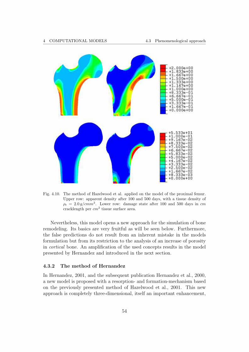
4 COMPUTATIONAL MODELS 4.3 Phenomenological approach
Fig. 4.10. The method of Hazelwood et al. applied on the model of the proximal femur.Upper row: apparent density after 100 and 500 days, with a tissue density ofρt = 2.0 g/cmm3. Lower row: damage state after 100 and 500 days in cmcracklength per cm2 tissue surface area.
Nevertheless, this model opens a new approach for the simulation of boneremodeling. Its basics are very fruitful as will be seen below. Furthermore,the false predictions do not result from an inherent mistake in the modelsformulation but from its restriction to the analysis of an increase of porosityin cortical bone. An amplification of the used concepts results in the modelpresented by Hernandez and introduced in the next section.
4.3.2 The method of Hernandez
In Hernandez, 2001, and the subsequent publication Hernandez et al., 2000,a new model is proposed with a resorption- and formation-mechanism basedon the previously presented method of Hazelwood et al., 2001. This newapproach is completely three-dimensional, itself an important enhancement,
54

4 COMPUTATIONAL MODELS 4.3 Phenomenological approach
t=0
t=T
t>T
t>T +TI
t=T +T +TI F
t> σ
R
R
R
R
old bone tissueresorption unitformation unitnew bone tissue
Fig. 4.11. An abstraction of the progression of a single BMU in remodeling equilibrium(resorbed tissue exactly replaced). Note the different time states in the remod-eling process.
and takes into account the process of mineralization. It was developed in thecontext of pharmaceutical treatment of osteoporosis, a bone disuse causingan enormous social damage. Therefore, mechanical aspects are neglectedand the simulation is concentrated on changes in bone mineral density dueto changes in the origination frequency. The latter term, the originationfrequency for, is defined as the number of BMUs newly appearing the internalsurface of a certain reference volume and time interval. This is to the contraryof the activation frequency which describes the number of BMUs passingthrough a certain cross section. A direct relation of these two terms can begiven by (Hernandez et al., 1999; Hernandez, 2001)
for =fa
dBMUvBMUσ(4.53)
with the activation frequency fa, the BMU-width dBMU , the BMU progres-sion rate, or velocity vBMU , and the lifespan σ. These values have beenintroduced in section 3.3 and refer to the geometry of the cell units whichcarry out internal remodeling.
A very elaborate model of the geometrical issues of the remodeling pro-cess, i.e., the microstructural process of BMU-progression, is used in thismethod. In figure 4.11, a sequence of picture shows the full replacement oftissue at a certain site carried out by a single BMU. For simplicity, only atrench as in trabecular remodeling is depicted. The tunnel in case of cor-tical bone follows the same principles. As an abstraction, all constituents
55

4 COMPUTATIONAL MODELS 4.3 Phenomenological approach
are presented as small squares. Note that these pictures represent remodel-ing in equilibrium, which takes place permanently and is not dedicated tomechanical adaptation but to damage removal and metabolic items. Theobservation, that remodeling is in equilibrium, is simply deduced from thefact that exactly the same amount of tissue is formed as previously resorbed.Nevertheless, these pictures give an insight into the spatial and temporalaspects of BMU-progression.
At a certain point in time, t = 0, a BMU is originated —for whateverreason— at the site, which is presented in this figure. Immediately afterorigination, it begins with resorption. Therefore, the first team of osteoclaststrenches a first hole into the tissue by resolving the organic and inorganicparts of bone matrix. In a second instant, the next unit of osteoclasts appearswhile the first has progressed by a certain length due to its progression ratevBMU . In the same manner, the whole resorbing part of the BMU digsthrough the tissue needing the time TR to pass completely the initial point.Now, it travels further leaving a gap behind which is caused by the internalchange from osteoclast to osteoblast activity. After this reversal period haspassed —now at point TR+TI in total time—, the first tissue forming unit ofosteoblasts appears where the BMU has initially started. In the same way asthe resorbing units, they travel while forming new osteoid and throughout theformation period TF new units appear at the initial point. This cell-complextrenches through the tissue surface, limited by its lifespan σ. If this timehas passed after origination, i.e., now t = σ, the first resorption unit stopsits activity and the cells disappear. Therefore, the distance, a BMU reachesis determined by this value. The other resorbing and forming cells keep onperforming their task until they meet the same fate and stop progressing.
Hence, in the spatial distance of σ vBMU the whole process stops and theactivity of this single BMU is terminated. Recall the remodeling volume ratesintroduced in section 3.3 due to BMU-geometry for cortical and cancellousbone and defined in equations (3.1). These values, Vcort and Vcanc for corticaland cancellous bone, respectively, can now be employed in order to determinethe remodeled tissue volume.
The total amount of remodeled volume is given by the term σVc as clearlyshown in picture 4.11. Mathematically more precise is the expression
Vc =
∫ t
t−σVc(t
′)dt′
with the index c presenting either cancellous or cortical bone. Working nowwith BMU-densities NBMU instead of single BMUs, in order to be consistentwith the principles of continuum mechanics, the above expression can be
56

4 COMPUTATIONAL MODELS 4.3 Phenomenological approach
modified to˙Vc(t)
VT=
∫ t
t−σNBMU(t′)dt′Vc(t) ,
which is the change of remodeled volume density in terms of the change ofBMU-density, NBMU , where the volume change per single BMU is assumedto be independent throughout its lifespan. Note that the fraction on the leftside of the above expression describes the change of tissue volume densitywhich is identical with a change in bone volume fraction VB/VT .
Now this change of volume is separated for resorption and formation,since a non-equilibrated remodeling process requires to distinguish them.Assuming that the BMU-density can change throughout the process, oneends up with the expression
˙(VBVT
)(t) =
∫ t−TR−TI
t−TR−TI−TF
(∫ t′
t′−σNBMU(t′′)dt′′
)Fb(t
′)dt′
−∫ t−TR
t
(∫ t′
t′−σNBMU(t′′)dt′′
)Fc(t
′)dt′ . (4.54)
By means of equation (4.54), the rate of change of bone volume fraction at thetime point t is fully defined by the history of rate of changes in BMU-densityvarying through the lifespans and the formation and resorption periods. Inother words, the inner integral provides the number of BMUs per volume unitin formation (resorption) at a time point t′, whereas the integration over theall t′ throughout the formation (resorption) time yields the change of bonevolume fraction due to formation (resorption). In this expression two factorsFb and Fc have been introduced, which are defined as
Fb = fbVcTF
and Fc = fcVcTR
. (4.55)
Here, Vc is the volume change unit as defined earlier with c indicating corticalor cancellous bone. Furthermore, TF and TR are the formation and resorp-tion periods, respectively, and the factors fb and fc are means to regulatethe amount of formed and resorbed bone, i.e., they are equal in remodelingequilibrium.
The driving force in this mechanism is the change of BMU-density whichis related to the origination frequency by
NBMU = forSv (4.56)
57

4 COMPUTATIONAL MODELS 4.4 Discussion
with the available specific surface Sv, due to Martin, 1984, a function of theporosity, formulated in equation (4.10) and depicted in figure 4.2.
Since mechanical items are neglected in this analysis, a relation between amechanical stimulus and the origination frequency is not given. This impor-tant value which causes the changes in BMU-density and therefore regulatesthe remodeling process, is simply set constant or varied as a response topharmaceutics.
Next to this enhanced three-dimensional model of BMU-progression, thismodel contains the evolution of the degree of mineralization which is newin computational bone remodeling. As pointed out in section 2.4, the newlyproduced bone tissue is purely organic (mainly collagen) and calcifies imme-diately through a period known as the primary mineralization period whichis of the order of some hours to a few days. From the yielded ash fractionα0 on, the second mineralization period begins, which is a saturation processduring many years and asymptotically tending to a maximal degree αmax.Confer figure 2.4 for a graphical presentation of these processes.
As described in section 2.5, the degree of mineralization plays an impor-tant role in the context of mechanical properties. Indeed, its impact on theYoung’s modulus is of a comparable order as the bone volume fraction, asclearly stated in equation (2.13), here repeated for sake of clarity
E = 84.37(VBVT
)2.58
α2.74 (4.57)
with the unit GPa.How the ash fraction exactly evolves in time is not presented. Unfortu-
nately, the integral equation (4.54) is not given either and had to be extractedfrom the rather cumbersome source code in the appendix to Hernandez, 2001.Nevertheless, the mechanically important aspects of this model are knownby now. A further presentation of the remaining concepts of the methodwould be distracting since they lead to medical treatments of osteoporosis.Numerical results in applying this model on one-element test cases can befound in Hernandez et al., 2000, Hernandez, 2001, Hernandez et al., 2001a,Hernandez et al., 2003, and will not be repeated here.
4.4 Discussion
In the above summary of computational methods for the simulation of adap-tive bone remodeling, two different strategies to simulate bone remodelinghave been presented, a mechanical and a phenomenological approach. In themechanical approach, the aim was to define a mathematical law describing
58

4 COMPUTATIONAL MODELS 4.4 Discussion
the evolution of density as a direct response to changes in the mechanical en-vironment. Therefore, the observation that bone is capable of adapting itselfto changes in applied loads and, furthermore, aligning its internal struc-ture with principle stress directions in a comparable continuum, was directlytranslated into mathematical formulations. This way is well-described withthe term of adaptive elasticity . The results of numerical simulations appearrelatively precise considering the enormous abstraction used to define themodels. One the other hand, it has to be clarified that, on the way froma totally fictitious initial situation (uniformly distributed density) to an un-stable solution —away from realistic results—, the internal structure of theproximal femur could be meanwhile reproduced. Therefore, these models arestill far away from a reliable algorithm which could be generally used in orderto predict results of internal bone remodeling.
The second line, the phenomenological approach, is much newer and hasbeen initiated by the method presented in Hazelwood et al., 2001. Here,the basic concept is to construct a model based on microstructural effects.Therefore, the spatial and temporal aspects of BMU-progression are consid-ered. In fact, the geometry of single BMUs has been used based on exper-imental measurements. Furthermore, the lifespan and remodeling periods(resorption, reversion, and formation) are employed leading to a delay inthe remodeling response as observed in reality. Hence, these models strictlyobey the A-R-F sequence (activation, resorption, formation, cf. section 3.3)which means that remodeling can only start when BMUs are activated by acertain stimulus (or as a permanent, homeostatic activity) and begins withresorption before formation can take place. Unfortunately, neither of the twomodels presented in the context has been used to simulated a full structure,such as the proximal femur model. Note that the application of the model ofHazelwood et al. on the femur was carried out in this work only and is nottaken from literature. The method of Hazelwood et al. was only used fora single test-element in order to observe its behavior in different load casesand its sensitivity to parameter changes. The latter method of Hernandezhas been additionally used to reproduce clinical results of changes in bonemineral density throughout osteoporosis and its therapy. Although a goodfit to data was produced, the changes in mechanical properties of a wholestructure have not been tested.
In order to go a step further in the evolution of algorithms on bone remod-eling, a new attempt —evidently based on previously developed concepts—will be proposed in the following chapter.
59

5 PROPOSITION OF A NEW MODEL
Fig. 5.1. Schematic representation of the remodeling algorithm proposed. The strain-based stimulus Y is the driving force, which causes a damage increase, controlsthe BMU-birthrate and focal bone balance, and the evolution of the fabric ten-sor. Furthermore, the equilibrium state ξ∗ accommodates to the stimulus. Both,birthrate and balance, determine in a history-dependent process the amount ofresorbed and formed tissue, which themselves cause damage removal and in-fluence on the time-dependent process of mineralization. The new bone vol-ume fraction, mineralization, damage state, and fabric tensor determine theanisotropic material stiffness C of bone tissue.
5 Proposition of a new model
The following chapter is taken from the Materials and Methods-section of a first version of a published article. Yet unknown is,whether it will be one article containing the full model or two, di-vided in an isotropic and an anisotropic model. Nevertheless, at leastone article will be submitted for publication in the Journal of Biome-chanics from the authors T. Rueberg, J.M. Garcıa, and M. Doblare.
In order to integrate this section into the whole document, addi-tional comments or supplements will be given either in brackets,[ ], or—in case of longer supplements— indented and in small fonts (thesame format as this preamble).
The model proposed in this work simulates the adaptation of the internalstructure of bone in terms of bone volume fraction and alignment of principlematerial directions as a response to the mechanical environment consideringdamage evolution and mineralization.
Actually, we assume a strain-based, anisotropic stimulus tensor Y, which
60
5 PROPOSITION OF A NEW MODEL 5.1 Definition of internal scalar variables
is controlling the BMU-birthrate. Furthermore, microdamage accumulationis driven by the same stimulus and in function of the load cycle number.The deviation of a functional of Y from an equilibrium state ξ∗ determinesthe relation of the internal cell-activities, the so-called focal bone balance,which regulates whether the amount of formed tissue shall be less, equal to,or more than the amount of resorbed tissue. This reference stimulus ξ∗ it-self is dependent on the applied stimulus in the sense, that it accommodatesto it in the long run. The changes in bone volume fraction due to resorp-tion and formation of tissue are determined by integrating over the historyof the birthrate while taking into account the BMU-lifespan and the focalbone balance. These resorption and formation quantities diminish damage,i.e., damage is reduced due to remodeling. In fact, we assume that dam-age removal is an important purpose of bone remodeling and, therefore, thestate of damage —determined by damage increase due to strain exposure anddamage decrease due to microcrack removal— affects on the BMU-birthrate.Moreover, the time-dependent process of mineralization is influenced by re-sorption and formation increments. Porosity is uniquely defined by the bonevolume fraction and thus the specific surface area Sv is calculated, which hasan impact on the birthrate, too.
Bone anisotropy is considered by means of the fabric tensor H, whichevolves in response to the stimulus tensor Y. In a long-term analysis italigns its principle axes with those of the applied strain state ε.
The anisotropic material stiffness C is finally determined by the bonevolume fraction, the degree of mineralization, the state of damage, and thefabric tensor. In order to close the cycle, the state of strain depends on theapplied load and geometry of the Finite Element model, and its constitutivelaw, which is the result of the previously described procedure.
In the following subsections, each step of the model is explained in de-tail. At first, we introduce the internal scalar variables that characterizebone tissue as a structural material. Next, the temporal evolution of theseindependent variables will be determined as functions of mechanical and bi-ological factors. And, finally, an extension to anisotropy will be provided.
5.1 Definition of internal scalar variables
Bone is a composite of tissue matrix and pores, where the latter are mainlyfilled with marrow, blood vessels, and nerves, all of which are mechanicallyinsignificant with respect to the rigid matrix. This structure can be quan-tified through the subdivision VT = VB + VV , where VB and VV refer to thebone tissue and void or pore subvolumes, respectively. VT denotes the totalvolume of analysis which is invariant in internal remodeling. The tissue ma-
61

5 PROPOSITION OF A NEW MODEL 5.1 Definition of internal scalar variables
trix is composed of inorganic (mineral) and organic (mainly collagen) parts,represented by the volume measures VM and VO, respectively. Furthermore,we assume a certain amount of tissue to be damaged (VD), such that [cf. thevolume subdivision introduced in sections 2.1 and 2.2]
VT = VB + VV = VM + VO + VD + VV . (5.1)
Therefore, the temporal evolution of these subvolumes is in the main focusof this internal bone remodeling theory. With this objective, we define asindependent variable the bone volume fraction vb, defined as
vb =VBVT
, (5.2)
which can be measured experimentally and has a significant impact on themechanical behavior. With this variable, the porosity p can be directly ex-pressed as
p =VVVT
= 1− vb . (5.3)
The second independent variable that we employ in order to characterizethe degree of mineralization is the ash fraction α (Hernandez, 2001;Martin etal., 1998), which is defined as the quotient of mineral mass mM (also termedash mass, since it results after the organic constituents have been evaporatedin a furnace) and the dry mass, which is the sum of mineral and organicmass, md = mM +mO. Hence,
α =mM
mM +mO
=ρMVM
ρMVM + ρOVO, (5.4)
where ρM and ρO refer to the densities of the mineral and organic parts,respectively.
Note that the apparent density ρ, the basic variable in the many internalbone remodeling models (Jacobs, 1994;Martin et al., 1998), can be relatedto the bone volume fraction by ρ = vbρt, where ρt is the tissue density,i.e., the density of a fictitious bone without porosity. Evidently, the tissuedensity depends on the degree of mineralization, since the mineral part hasa much higher specific weight than the organic part. A linear approximationthereto is given by Hernandez (Hernandez, 2001;Hernandez et al., 2001a) asρt = 1.41 + 1.29α (in g/cm3) in good correlation with experimental data. Inseveral experimental outcomes (ibidem), the elastic properties of bone showedbetter correlation with the bone volume fraction vb and mineralization α thanwith apparent density ρ.
62
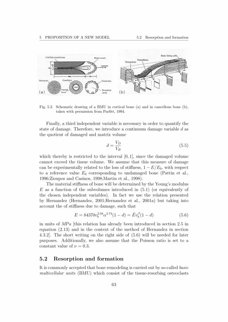
5 PROPOSITION OF A NEW MODEL 5.2 Resorption and formation
Fig. 5.2. Schematic drawing of a BMU in cortical bone (a) and in cancellous bone (b),taken with permission from Parfitt, 1994.
Finally, a third independent variable is necessary in order to quantify thestate of damage. Therefore, we introduce a continuum damage variable d asthe quotient of damaged and matrix volume
d =VDVB
(5.5)
which thereby is restricted to the interval [0, 1], since the damaged volumecannot exceed the tissue volume. We assume that this measure of damagecan be experimentally related to the loss of stiffness, 1−E/E0, with respectto a reference value E0 corresponding to undamaged bone (Pattin et al.,1996;Zioupos and Casinos, 1998;Martin et al., 1998).
The material stiffness of bone will be determined by the Young’s modulusE as a function of the subvolumes introduced in (5.1) (or equivalently ofthe chosen independent variables). In fact we use the relation presentedby Hernandez (Hernandez, 2001;Hernandez et al., 2001a) but taking intoaccount the of stiffness due to damage, such that
E = 84370v2.58b α2.74(1− d) = Evβb (1− d) (5.6)
in units of MPa [this relation has already been introduced in section 2.5 inequation (2.13) and in the context of the method of Hernandez in section4.3.2]. The short writing on the right side of (5.6) will be needed for laterpurposes. Additionally, we also assume that the Poisson ratio is set to aconstant value of ν = 0.3.
5.2 Resorption and formation
It is commonly accepted that bone remodeling is carried out by so-called basicmulticellular units (BMU) which consist of the tissue-resorbing osteoclasts
63

5 PROPOSITION OF A NEW MODEL 5.2 Resorption and formation
and the tissue-forming osteoblasts in a coupled way. Furthermore, these cellunits proceed in a strict order at a fixed point of observation: after beingactivated they first resorb bone tissue for a time period termed resorption pe-riod (TR), and, after a reversal time (TI) has passed by, the formation period(TF ) starts. This unchangeable sequence has been termed A-R-F sequence(activation, resorption, formation) by several authors (Parfitt, 1994;Martinet al., 1998) and results in the geometrical constellation given in figure 5.2.The lifespan of a BMU is denoted by σ and refers to the time span the firstappearing osteoclasts are active. This is a useful definition, since σ is di-rectly related with the maximal distance that a BMU travels by means of itsprogression speed vBMU , the so-called BMU-rate. Note that these measuresbelong to a three-dimensional histomorphometry and thereby consider thespatial and temporal progression of BMUs in a three-dimensional space.
The processes of resorption and formation are not only coupled but alsoassumed to take place permanently, even in remodeling equilibrium. Thiscoincides with microdamage removal and calcium provision as purposes ofbone remodeling other than the mechanical adaptation and has been observedexperimentally (Buckwalter et al., 1995). The rate of change of the bonevolume fraction can thus be expressed by
vb = vF − vR (5.7)
where vF and vR are the changes contributed by formation and resorption,respectively. In remodeling equilibrium, vb = 0 and, therefore, vF = vR, i.e.,formed and resorbed tissue quantities are equal.
These changes in bone volume fraction are functions of the number ofBMUs currently active which can be represented by the BMU-density NBMU ,defined as the number of BMUs per reference volume (BMUs/mm3). Onceactivated, a BMU moves for the distance σvBMU . In detail, at a certain siteit stays through TR in resorption, needs TI for the change from osteoclast toosteoblast activity, and remains finally during TF in formation. This complexthree-dimensional and history-dependent process can be formulated with thefollowing expression
V (t) =
∫ LBMU
0
(∫ t′
t′−σNBMU(t′′)dt′′
)dA(x)
dtdx , (5.8)
where dx is a way increment in direction of progression of a BMU with lengthLBMU . dA(x)/dt describes how a BMU extends in transversal direction and∫ t′t′−σ NBMU(t′′)dt′′ determines the number of BMUs that are active in the
considered time.
64

5 PROPOSITION OF A NEW MODEL 5.2 Resorption and formation
We assume that the rate of remodeling in transversal direction, i.e., nor-mal to the main direction of progression, is constant and independent of thespatial variable x. Distinguishing between resorption and formation due tothe different velocities, the transverse remodeling rate will be expressed as
dA(x)
dt=
ABMU
TRfc if resorption
ABMU
TFfb if formation
(5.9)
with TR and TF the resorption and formation periods, respectively, fb and fcrepresent the level of osteoblast and osteoclast activity, and finally, ABMU isthe cross-sectional area of a BMU.
Because the geometry of a cortical and cancellous BMUs is completelydifferent (figure 5.2), we consider different cross sections ABMU . Actually, thenewly refilled bone in cortical tissue has a cylindrical shape (called osteon),whereas the equivalent in cancellous tissue is of a rather irregular shape whichcan be approached by a half-cylinder with elliptic cross-section (termed hemi-osteon by Parfitt, 1994). As in Hernandez, 2001, we assume the geometriesas depicted in figure 5.3, which can be formulated by [equivalently to section3.3]
ABMU =
(d2O
4− d2
H
4
)π in cortical bone
π
4dE dBMU in cancellous bone.
(5.10)
Furthermore, dx is directly related to the rate of progression of a BMUby dx = vBMU dt. If we combine equations (5.8) to (5.10), the volume ofremoved/refilled bone can be obtained as [cf. equation (4.54) and figure 4.11for a similar approach to these equations]
vF (t) =
∫ t−TR−TI
t−TR−TI−TF
(∫ t′
t′−σNBMU(t′′)dt′′
)ABMU
TFfb(t
′)vBMUdt′ (5.11a)
vR(t) =
∫ t−TR
t
(∫ t′
t′−σNBMU(t′′)dt′′
)ABMU
TRfc(t
′)vBMUdt′ . (5.11b)
Equations (5.11) describe the changes in bone volume fraction at time t infunction of changes in BMU-density which took place in the recent history.
A constant birthrate NBMU leads to a constant number of active BMUs,since their life span is assumed to be equal. Together with fb = fc = 1 (seebelow), equations (5.11) then lead to
vR = vF = NBMUσABMUvBMU , (5.12)
65

5 PROPOSITION OF A NEW MODEL 5.2 Resorption and formation
Haversiandiameter
d H
Rate ofprogression
vBMU
osteonal diameter do
BMU width dBMU
Rate ofprogression
v
Erosiondepth
d
BMU
e
Fig. 5.3. A model of the tissue volume unit a single BMU remodels in cortical (left) andcancellous (right) bone tissue per time unit, adapted from Hernandez, 2001.
which is the equilibrium state in remodeling. Actually, the right hand sideof equation (5.12) is the product of the number of active BMUs NBMU andσABMUvBMU , the amount of volume that a single BMU remodels during itslife time.
Changes in BMU-density NBMU , i.e., changes in the number of BMUscurrently active, result either from exceeding their life span σ in form ofa decrease in number, or from the origination of new BMUs in form of anincrease. Whereas the former event (also referred to as apoptosis) takesplace automatically, the latter is controlled by the origination frequency for(or birthrate) and the available surface area per reference bone volume SVin such a way that
NBMU = forSV . (5.13)
The dependence of the BMU birthrate on the surface density, SV , indi-cates that remodeling only occurs on the tissue surface. The value of theavailable surface depends directly on the porosity, related by a quintic poly-nomial as shown by Martin, 1984[cf. equation (4.10)].
The second factor, that determines the occurrence of new BMUs, isthe origination frequency, which is controlled by different factors, such asmetabolical, mechanical, etc.
It is commonly known from experimental and clinical results (Vico et al.,2000;Buckwalter et al., 1995), that the bone volume fraction decreases in astate of disuse. Furthermore, it is suggested that microdamage caused byfatigue activates remodeling in order to repair the damaged regions (Martin,2002;Martin, 2003).
Here, we assume that the origination frequency depends on a biologicalfactor, a mechanical stimulus and the accumulative damage, following the
66

5 PROPOSITION OF A NEW MODEL 5.2 Resorption and formation
inhibitory theory proposed by Martin, 2000 [cf. section 3.4 for more detailson the inhibitory concept and the purposes of remodeling]. He assumed thata signal is permanently produced in the cellular network of osteocytes andbone-lining cells that is strain- or stress-generated and transmitted throughthis network, which impedes BMUs from activation. Hence, any perturba-tion in the reception of such a signal causes a certain degree of activation.Either the generation of the signal is disturbed by a low strain level or itstransmission is hindered by microcracks disrupting the connectivity of thecellular network. In this sense, we propose
for = fbio(1− s) (5.14)
where fbio is a certain biological factor and s the normalized level of thereceived signal. Now, s is a function of the state of damage and the appliedmechanical strain.
The strain influence is determined by a scalar quantity, which representsthe daily strain history and, therefore, depends on the strain level and thenumber of cycles for each load case i, following the stimulus proposed byCarter (Jacobs, 1994) [cf. also section 4.2.2]
ξ =
(∑i
Niεmi
)1/m
. (5.15)
Ni denotes the number of load cycles and the level of the applied strain εi withi indicating each load case, where the influence of strain and cycle number isweighted by the exponent m. Typically, m = 4, as observed in experiments(cf. Carter and Beaupre, 2001), such that the level of the applied strain hasa much higher impact than the number of cycles. The used strain functionalis defined as
ε =
√2U
E(5.16)
with the strain energy density U = ε : C : ε. Note that the here presentedmethod depends on the load history as clearly stated in (5.11)†.
Now, the dependence of the received signal level s on the mechanicalstimulus ξ and the damage variable d will be proposed as
s(ξ, d) =ξ2
ξ2 + c2(1− d)k (5.17)
†Therefore, the reordering and grouping of load cases as introduced by Jacobs, 1994,which results in a simplification of the stimulus, is not admissible in this model.
67
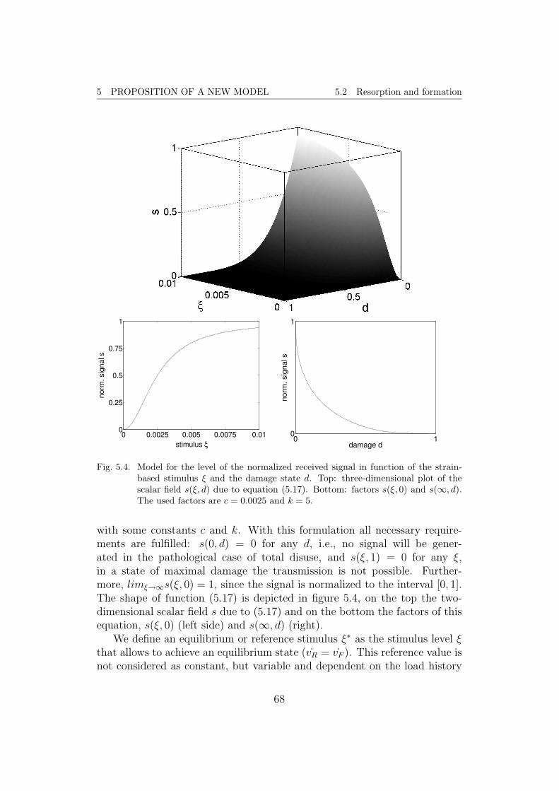
5 PROPOSITION OF A NEW MODEL 5.2 Resorption and formation
0 0.0025 0.005 0.0075 0.010
0.25
0.5
0.75
1
stimulus ξ
norm
. sig
nal s
0 10
1
damage d
norm
. sig
nal s
Fig. 5.4. Model for the level of the normalized received signal in function of the strain-based stimulus ξ and the damage state d. Top: three-dimensional plot of thescalar field s(ξ, d) due to equation (5.17). Bottom: factors s(ξ, 0) and s(∞, d).The used factors are c = 0.0025 and k = 5.
with some constants c and k. With this formulation all necessary require-ments are fulfilled: s(0, d) = 0 for any d, i.e., no signal will be gener-ated in the pathological case of total disuse, and s(ξ, 1) = 0 for any ξ,in a state of maximal damage the transmission is not possible. Further-more, limξ→∞s(ξ, 0) = 1, since the signal is normalized to the interval [0, 1].The shape of function (5.17) is depicted in figure 5.4, on the top the two-dimensional scalar field s due to (5.17) and on the bottom the factors of thisequation, s(ξ, 0) (left side) and s(∞, d) (right).
We define an equilibrium or reference stimulus ξ∗ as the stimulus level ξthat allows to achieve an equilibrium state (vR = vF ). This reference value isnot considered as constant, but variable and dependent on the load history
68
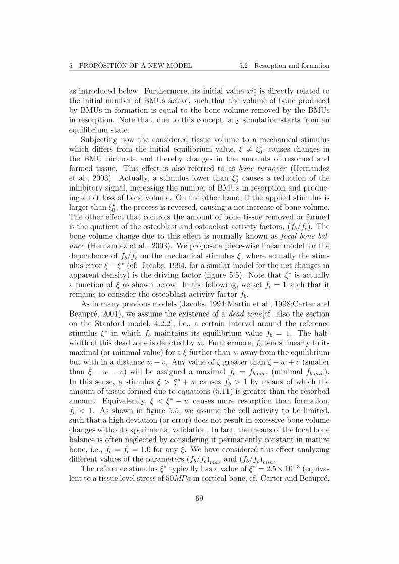
5 PROPOSITION OF A NEW MODEL 5.2 Resorption and formation
as introduced below. Furthermore, its initial value xi∗0 is directly related tothe initial number of BMUs active, such that the volume of bone producedby BMUs in formation is equal to the bone volume removed by the BMUsin resorption. Note that, due to this concept, any simulation starts from anequilibrium state.
Subjecting now the considered tissue volume to a mechanical stimuluswhich differs from the initial equilibrium value, ξ 6= ξ∗0 , causes changes inthe BMU birthrate and thereby changes in the amounts of resorbed andformed tissue. This effect is also referred to as bone turnover (Hernandezet al., 2003). Actually, a stimulus lower than ξ∗0 causes a reduction of theinhibitory signal, increasing the number of BMUs in resorption and produc-ing a net loss of bone volume. On the other hand, if the applied stimulus islarger than ξ∗0 , the process is reversed, causing a net increase of bone volume.The other effect that controls the amount of bone tissue removed or formedis the quotient of the osteoblast and osteoclast activity factors, (fb/fc). Thebone volume change due to this effect is normally known as focal bone bal-ance (Hernandez et al., 2003). We propose a piece-wise linear model for thedependence of fb/fc on the mechanical stimulus ξ, where actually the stim-ulus error ξ− ξ∗ (cf. Jacobs, 1994, for a similar model for the net changes inapparent density) is the driving factor (figure 5.5). Note that ξ∗ is actuallya function of ξ as shown below. In the following, we set fc = 1 such that itremains to consider the osteoblast-activity factor fb.
As in many previous models (Jacobs, 1994;Martin et al., 1998;Carter andBeaupre, 2001), we assume the existence of a dead zone[cf. also the sectionon the Stanford model, 4.2.2], i.e., a certain interval around the referencestimulus ξ∗ in which fb maintains its equilibrium value fb = 1. The half-width of this dead zone is denoted by w. Furthermore, fb tends linearly to itsmaximal (or minimal value) for a ξ further than w away from the equilibriumbut with in a distance w+ v. Any value of ξ greater than ξ +w+ v (smallerthan ξ − w − v) will be assigned a maximal fb = fb,max (minimal fb,min).In this sense, a stimulus ξ > ξ∗ + w causes fb > 1 by means of which theamount of tissue formed due to equations (5.11) is greater than the resorbedamount. Equivalently, ξ < ξ∗ − w causes more resorption than formation,fb < 1. As shown in figure 5.5, we assume the cell activity to be limited,such that a high deviation (or error) does not result in excessive bone volumechanges without experimental validation. In fact, the means of the focal bonebalance is often neglected by considering it permanently constant in maturebone, i.e., fb = fc = 1.0 for any ξ. We have considered this effect analyzingdifferent values of the parameters (fb/fc)max and (fb/fc)min.
The reference stimulus ξ∗ typically has a value of ξ∗ = 2.5×10⁻³ (equiva-lent to a tissue level stress of 50MPa in cortical bone, cf. Carter and Beaupre,
69

5 PROPOSITION OF A NEW MODEL 5.3 Mineralization
ξ∗ξ∗−w ξ∗+w+vξ
ξ∗+wξ∗−w−v1.0
(f /f )b c
max
min
(f /f )
(f /f )
b c
b c
Fig. 5.5. Model for the focal bone balance.
2001). But this value seems to be only applicable to weight-baring bones(e.g., femur, tibia), whereas fewer charged bones (e.g. the protective flatbones such as cranium, scapula), cannot be subjected to such a high value.Bone mass is maintained in either types of bone, because this reference stim-ulus is dependent on the loading history, modifying its value adaptive way.This idea is similar to the concept of cellular accommodation as proposed byTurner, 1999. We therefore assume, that the reference stimulus ξ∗ adapts tothe applied stimulus ξ, formulated by the asymptotic function
ξ∗(ξ, t) = ξ − (ξ − ξ∗0)e−ϕt , (5.18)
where ξ∗0 denotes the initial reference stimulus and the parameter ϕ controlsthe velocity of adaption. By means of this model, a permanently low or highstimulus does not yield excessive remodeling. Furthermore, it maintains theapplicability of our method to a variety of bone types.
5.3 Mineralization
As time proceeds the newly formed tissue, which is primarily collagen, calci-fies and the volume of osteoid is converted into mineral [more details on theprocess of mineralization are given in section 2.4]. Over the first few daysof mineralization, crystals appear throughout the mineralized bone, occupy-ing the space of water. This transformation process succeeds rapidly at thebeginning and retards like a saturation process. It is generally divided intotwo phases, the fast primary phase which proceeds within a few days (Her-nandez, 2001;Hernandez et al., 2001a) and the slow secondary phase whichtakes some years of time. The primary phase yields at about 60 % of themaximal mineral content. Here, we assume that the primary phase occurssimultaneously, and it remains to model the secondary phase starting fromthe result of the primary phase. Employing the ash fraction α as the typical
70

5 PROPOSITION OF A NEW MODEL 5.3 Mineralization
0 2 4 6
time [years]
ash
fract
ion
α [/]
secondary mineralization phase
primary mineralization phase
0
α0
αmax
Fig. 5.6. The evolution of the ash fraction in time. Here, the parameter κ is chosen suchthat after 6 years 50 % of the second mineralization phase have been passed.
measure for the degree of mineralization and already defined in (5.19), wepropose the model
α(t) = αmax + (α0 − αmax)e−κt , (5.19)
where α0 denotes the ash fraction resulting from the primary phase and αmaxis the maximal degree [cf. also equation (2.7)]. The constant κ determinesthe velocity of this process. In figure 5.6 a graphical presentation is given,depicting the two phases. It has been shown in Hernandez, 2001, and Her-nandez et al., 2001a, that the degree of mineralization is not correlated withthe bone volume fraction.
Now, an averaged ash fraction α is introduced, considering the impact ofremodeling on the mineralization
α(t) =vb,0α(t) +
∫ t0
(vF (τ)α(t− τ)− vR(τ)α(τ)) dτ
vb(t). (5.20)
with the bone volume rate of changes vF and vR due to equation (5.11).The averaged ash fraction thus consists of the evolution of the mineral con-tents of the initial bone volume fraction vb,0, the contribution of the newlyformed tissue (convolution integral), and an approximation of the reductionby resorption (since it is not known which ash fraction the resorbed tissuepossessed, the average α is used). In order to reduce the numerical effort, anexpression for the averaged ash fraction at time t+ ∆t is found to be
α(t+ ∆t) =α(t)(vb(t)e
−κ∆t −∆vR) + ∆vFα0 + αmax(1− e−κ∆t)vb(t)
vb(t+ ∆t)
+(1− e−κ∆t)
∫ t0vR(αmax − α(τ))dτ
vb(t+ ∆t)(5.21)
71

5 PROPOSITION OF A NEW MODEL 5.4 Damage
where ∆vF and ∆vR approximate the amounts of tissue formed and resorbed,respectively, in the time interval [t, t+∆t]. Apart from the remaining integral,which has to be stored separately, all values in (5.21) are known in each timeincrement of the simulation.
The way of getting (5.21) from (5.20) by incrementing the time fromt to t+ ∆t can be found by
α(t+ ∆t) =P0α(t+ ∆t) +
∫ t+∆t0 PF (τ)α(t+ ∆t− τ)− PR(τ)α(τ)dτ
P (t+ ∆t)
=P0[αmax + (α(t)− αmax)e−κ∆t]
P (t+ ∆t)
+
∫ t+∆t0 PF (τ)[αmax + (α(t− τ)− αmax)e−κ∆t]− VR(τ)α(τ)dτ
P (t+ ∆t)
=P0α(t)e−κ∆t + P0αmax(1− e−κ∆t) +
∫ t0 PF (τ)α(t− τ)dτe−κ∆t
P (t+ ∆t)
+
∫ t0 PF (τ)dτ(1− e−κ∆t)−
∫ t0 PR(τ)α(τ)dτ(1− e−κ∆t + e−κ∆t)P (t+ ∆t)
+
∫ t+∆tt PF (τ)α(t+ ∆t− τ)− PR(τ)α(τ)dτ
P (t+ ∆t)
=α(t)(P (t)e−κ∆t −∆PR) + αmax(1− e−κ∆t)(P0 +
∫ t0 PF − PR
α(τ)αmax
dτ)P (t+ ∆t)
+∆PFα0
P (t+ ∆t),
where the following property of model (5.19) has been used
α(t+ ∆t) = αmax + (α0 − αmax)e−κte−κ∆t
= αmax + (α(t)− αmax)e−κ∆t .
5.4 Damage
Bone tissue is often submitted to cyclic or fluctuating loads that causes anaccumulation of microstructural damage, which may culminate in the forma-tion and growth of cracks.
So far, a damage measure d has been introduced in equation (5.5) whichactivates remodeling by expressions (5.14) and (5.17). Now, the aim is todetermine an evolution law which is consistent with experimental results forthe in vitro damage behavior and combine it with the impact of remodelingon the damaged subvolume VD [cf. section 2.6 for more details on damage inbone].
72
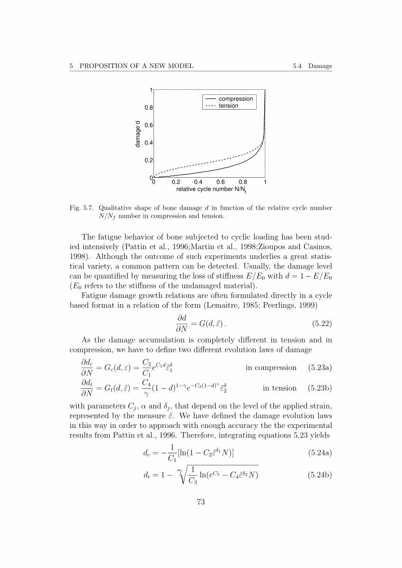
5 PROPOSITION OF A NEW MODEL 5.4 Damage
0 0.2 0.4 0.6 0.8 10
0.2
0.4
0.6
0.8
1
relative cycle number N/Nf
dam
age
d
compressiontension
Fig. 5.7. Qualitative shape of bone damage d in function of the relative cycle numberN/Nf number in compression and tension.
The fatigue behavior of bone subjected to cyclic loading has been stud-ied intensively (Pattin et al., 1996;Martin et al., 1998;Zioupos and Casinos,1998). Although the outcome of such experiments underlies a great statis-tical variety, a common pattern can be detected. Usually, the damage levelcan be quantified by measuring the loss of stiffness E/E0 with d = 1−E/E0
(E0 refers to the stiffness of the undamaged material).Fatigue damage growth relations are often formulated directly in a cycle
based format in a relation of the form (Lemaitre, 1985; Peerlings, 1999)
∂d
∂N= G(d, ε) . (5.22)
As the damage accumulation is completely different in tension and incompression, we have to define two different evolution laws of damage
∂dc∂N
= Gc(d, ε) =C2
C1
eC1dεδ1 in compression (5.23a)
∂dt∂N
= Gt(d, ε) =C4
γ(1− d)1−γe−C3(1−d)γ εδ2 in tension (5.23b)
with parameters Cj, α and δj, that depend on the level of the applied strain,represented by the measure ε. We have defined the damage evolution lawsin this way in order to approach with enough accuracy the the experimentalresults from Pattin et al., 1996. Therefore, integrating equations 5.23 yields
dc = − 1
C1
[ln(1− C2εδ1N)] (5.24a)
dt = 1− γ√
1
C3
ln(eC3 − C4εδ2N) (5.24b)
73

5 PROPOSITION OF A NEW MODEL 5.4 Damage
[the same result is given in equations (2.16)].The fatigue life expectation which is typically of the form
Nf = Cεδ . (5.25)
Setting d = 1 in one of the equations of (5.24) and solving for N = Nf , resultsin a comparable structure such that the parameters of equations (5.23) canbe determined by comparing the coefficients with experimental results. Wehave represented these equations (5.24) in figure 5.7, showing a similar shapeas the ones obtained by Pattin et al., 1996, in experiments .
All these expressions correspond to damage accumulation in a non-livingmaterial, but bone can repair itself, decreasing the damage level. In thissense, the main assumption that we have used is that the impact of remodel-ing on the damage state is assumed not to be targeted, i.e., a BMU might beoriginated due to damage influence as described above, but does not remodelselectively a damaged area. In other words, the damaged subvolume VD isuniformly distributed in the control volume.
So, recalling the definition of the damage variable d = VD/VB, showsthat it does not decrease in resorption, since both damaged and bone volumedecrease proportionally due to the assumption made. On the other hand,formation increases the bone tissue volume VB thus decreasing the quotient,i.e., the damage variable decreases as a result of formation. Since both,resorption and formation, take permanently place in a coupled way, an aux-iliary variable d = VD/VT is introduced in order to fully describe the matter.This variable decreases in resorption (as VD decreases) and stays constant information. Both variables, d and d, are related due to their definitions by
vb =d
d. (5.26)
Deriving now (5.26) with respect to time and considering the differentbehavior in resorption and formation (vb = vF − vR) yields the rate of changeof the damage variables due to remodeling
d = −vFd2
d(5.27a)
˙d = −vRd . (5.27b)
With equations (5.27a) (using d which evolves due to (5.27b)) and (5.23),the current state of damage can be fully determined. Note that both d and˙d in (5.27) are negative and damage thereby diminishes as a result of the
remodeling process.
74

5 PROPOSITION OF A NEW MODEL 5.5 Extension to anisotropy
5.5 Extension to anisotropy
So far, the isotropic model is fully defined. The extension of this model toa generalized anisotropic theory is performed by means of the principles ofcontinuum damage mechanics, using the ideas suggest by Doblare and Garcıa(Garcıa, 1999; Doblare and Garcıa, 2002). They interpret, from a mathemat-ical point of view, porosity as damage in magnitude and directionality, butdistinguish it from the actual microdamage due to cyclic loading [cf. section4.2.4 for the model of Garcıa and Doblare]. In this sense, a new variablehas to be introduced in order to characterize the structural orientation ofbone tissue. Therefore, we have chosen the fabric tensor as introduced byCowin, 1986 [and presented in detail in appendix B], which is a symmetricpositive definite second order tensor, with its principal axes coinciding withthe principal material directions.
In order to achieve a condense formulation, an anisotropic remodelingtensor will be introduced
H = vβ/4b H1/2 (5.28)
with the same exponent β as in equation (5.6) and H the fabric tensor, whichis normalized such that det(H) = 1. Using the methodotology developed byDoblare and Garcıa (Garcıa, 1999), the components of the compliance tensorC−1 in its principal directions can be given in terms of the principle valuesof remodeling tensor H and of the actual damage level d
1
EI=
1
E(1− d)
1
H4I
−νI IIEII
= −νII IEI
= − ν
E(1− d)
1
H2IH
2II
1
2GI II
=1 + ν
E(1− d)
1
H2IH
2II
,
(5.29)
where the material parameter E refers to the elastic modulus defined inequation (5.6) and ν = ν = 0.3 . Mutual exchange of the indices I, II, andIII in (5.29) yields the remaining components.
In order to derive an evolution law for the remodeling tensor H, or iden-tically for the fabric tensor H, we follow again the same steps that Doblareand Garcıa proposed (Garcıa, 1999). Initially, the mechanical stimulus con-sidered is the variable associated with H in terms of the free energy functionψ
Y =∂ψ(ε,H)
∂H= 2
(λ tr(H2ε)Hε+ 2µ(HεH)(Hε)
)(5.30)
75

5 PROPOSITION OF A NEW MODEL 5.5 Extension to anisotropy
with the Lame constants λ and µ which are evaluated with the same param-eters E and ν as above. In fact, this stimulus Y is directly related to thestrain energy density U (Garcıa, 1999).
So, we can define the remodeling criteria by means of this stimulus andbeing consistent with the isotropic conditions as shown in figure 5.5, thekernel of the dead zone can be defined by the expressions
gr = − 31/4√2E(1− d)(1− ω)
(∑i
Ni (Ji : Ji)m/4
)1/m
+ (ξ∗ − w) v3β/8b < 0
(5.31a)
gf =31/4√
2E(1− d)(1− ω)
(∑i
Ni (Ji : Ji)m/4
)1/m
− (ξ∗ + w) v3β/8b < 0 .
(5.31b)
The derivation of criteria (5.31) shall be outlined briefly. Thiswill be done for the case of resorption only, whereas in formation thesame methodotology applies. Starting now from the isotropic model’scondition
ξ > ξ∗ − w ,
which is the ’left border’ of the dead zone, one has just to insert thedefinition of ξ due to (5.15) and (5.16), such that
−
∑i
Ni
(√εi : C : εiE(1− d)
)m1/m
+ (ξ∗ − w) < 0 ,
where the dependencies of C and E on the bone volume fraction vbappear equally in nominator and denominator such that they canceleach other. The trace of the stimulus tensor Y can be related on theone hand to the strain energy by
ε : C : ε =12v−3β/4b tr(Y)
and on the other hand to the tensor J
tr2(Y) = 3J : J
in the isotropic case (ω = 0). With these relations the isotropic crite-rion for resorption can be expressed in terms of the tensor Y
gr = − 31/4√2E(1− d)
(∑i
Ni (Ji : Ji)m/4
)1/m
+ (ξ∗ − w) v3β/8b < 0 .
76

5 PROPOSITION OF A NEW MODEL 5.5 Extension to anisotropy
The final criterion (5.31a) can now be derived for an anisotropic anal-ysis (ω 6= 0) but starting from an isotropic case (dev(Y) = 0) whichyields the factor 1/
√1− ω and thereby the final expression.
Now, J is a tensor dependent on Y, where spherical and deviatory parts ofY are superposed in a convex combination with weighting parameter ωε[0, 1](Doblare and Garcıa, 2002)
J = (1− ω)1
3tr(Y)1 + ω dev(Y) = (1− 2ω)
1
3tr(Y)1 + ωY . (5.32)
In other words, if (5.31) are fulfilled, the bone focal balance is maintained,i.e., fb = fc = 1. But in case of gr = 0 (gf = 0), more tissue is resorbed(formed) than formed (resorbed). We therefore employ the same relationshipas depicted in figure 5.5, i.e, a piece-wise linear model with a dead zone ofwidth 2w, linear transition zones of width v and the restriction to a maximaland a minimal value fb,max and fb,min, respectively.
The evolution of the remodeling tensor H is now given using an associatedlaw like in standard plasticity (Doblare and Garcıa, 2002)
H = µr∂gr
∂Y+ µf
∂gf
∂Y(5.33)
with the side conditions
µr , µf ≥ 0 , gr , gf ≤ 0 , and µrgr + µfgf = 0 . (5.34)
Adjusting with the isotropic case, in which bone volume is determinedthrough vb, we can calculate the rates µj and, thereby, a full expression ofthe rate of change of H (Garcıa, 1999)
H =
∑i Ji : ω∑
i tr(H−2Ji : ωH)
3β
4vbvb , (5.35)
where ω is an auxiliary tensor resulting from ∂J/∂Y and defined as
ω = (1− 2ω)1
31⊗ 1 + ωI . (5.36)
1 is the second-order and I the fourth-order identity for cartesian tensors.It can be seen in (5.35) that H depends directly on the rate of change of
the bone volume fraction, given by vb. Although vb changes in dependenceof the load history (recall integral the expressions (5.11)), H and thereby theanisotropy change instantaneously in response to the current stimulus. Thisis based on the concept of BMUs being capable to steer in the appropriatedirection during all the time (Martin et al., 1998).
77

5 PROPOSITION OF A NEW MODEL 5.5 Extension to anisotropy
Note that the expression for the resorption criterion (5.31a) differsfrom the one employed by Garcıa and Doblare (Garcıa, 1999;Doblareand Garcıa, 2002). And, consequently, the evolution law for the re-modeling tensor is different, too. This part has been changed, sincethe formulation proposed by Garcıa and Doblare yielded a very highdegree of anisotropy in case of resorption (dependence on J−3 as canbe seen in (4.39) in section 4.2.4). Furthermore, a reduction of thestimulus in a given equilibrium situation led to an increase in thedegree of anisotropy which is not meaningful.
78
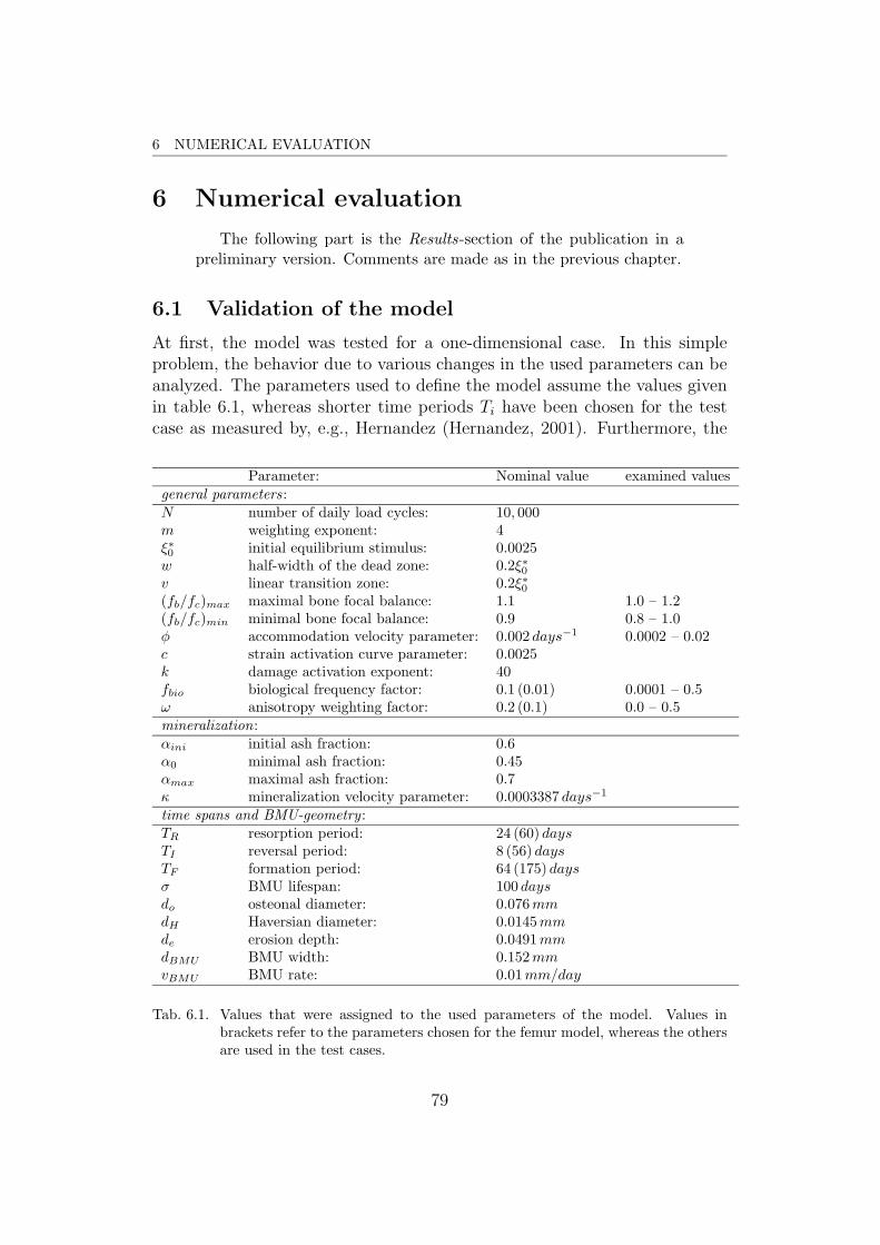
6 NUMERICAL EVALUATION
6 Numerical evaluation
The following part is the Results-section of the publication in apreliminary version. Comments are made as in the previous chapter.
6.1 Validation of the model
At first, the model was tested for a one-dimensional case. In this simpleproblem, the behavior due to various changes in the used parameters can beanalyzed. The parameters used to define the model assume the values givenin table 6.1, whereas shorter time periods Ti have been chosen for the testcase as measured by, e.g., Hernandez (Hernandez, 2001). Furthermore, the
Parameter: Nominal value examined valuesgeneral parameters:N number of daily load cycles: 10, 000m weighting exponent: 4ξ∗0 initial equilibrium stimulus: 0.0025w half-width of the dead zone: 0.2ξ∗0v linear transition zone: 0.2ξ∗0(fb/fc)max maximal bone focal balance: 1.1 1.0 – 1.2(fb/fc)min minimal bone focal balance: 0.9 0.8 – 1.0φ accommodation velocity parameter: 0.002 days−1 0.0002 – 0.02c strain activation curve parameter: 0.0025k damage activation exponent: 40fbio biological frequency factor: 0.1 (0.01) 0.0001 – 0.5ω anisotropy weighting factor: 0.2 (0.1) 0.0 – 0.5mineralization:αini initial ash fraction: 0.6α0 minimal ash fraction: 0.45αmax maximal ash fraction: 0.7κ mineralization velocity parameter: 0.0003387 days−1
time spans and BMU-geometry :TR resorption period: 24 (60) daysTI reversal period: 8 (56) daysTF formation period: 64 (175) daysσ BMU lifespan: 100 daysdo osteonal diameter: 0.076mmdH Haversian diameter: 0.0145mmde erosion depth: 0.0491mmdBMU BMU width: 0.152mmvBMU BMU rate: 0.01mm/day
Tab. 6.1. Values that were assigned to the used parameters of the model. Values inbrackets refer to the parameters chosen for the femur model, whereas the othersare used in the test cases.
79

6 NUMERICAL EVALUATION 6.1 Validation of the model
0 250 500 750 10000
0.2
0.4
0.6
0.8
1
0 250 500 750 10001
1.5
2
2.5
3x 10⁻³
time [days]
rem
odel
ing
incr
emen
ts
overload
disuse
∆ vF
∆ vR
Fig. 6.1. Left: bone volume fraction for different initial densities, ρ0 = 1.8 g/cm3, 1.0,and 0.3 (all with reference to an initial ash fraction of 0.6), and for states ofequilibrium ξ = ξ∗0 (solid line), overload ξ = 2ξ∗0 (-+-), and disuse ξ = 0 (-o-).Right: the evolution of the remodeling increments ∆vR and ∆vF due to theresorption and formation parts, respectively, in the same states of disuse andoverload.
biological factor controlling the BMU birthrate fbio has been set ten timeshigher than the order of magnitude used by Hernandez (Hernandez, 2001).This has been done in order to reduce the time of computation. The valuesgiven in parentheses are more realistic [ibidem] and have been used for theanalysis of the proximal femur (see below). All test calculations simulatedthe behavior in 1000 days, where this time scale is of minor significancedue to the shorter time periods chosen. The initial state was supposed tobe equilibrated, i.e., with a constant birthrate and a focal bone balancefb = fc = 1.0. In fact, the initial values were chosen as if a stimulus ofξ = ξ∗0 had been applied before the begin of the calculation, for time t < 0.Therefore, the initial number of BMUs is uniquely defined.
state variables:vb bone volume fraction d continuum damage variableα averaged ash fraction H anisotropic remodeling tensorNBMU BMU density ξ∗ reference stimulusintermediate variables:ε strain measure d auxiliary damage variableξ applied stimulus for origination frequencySv available tissue surface s norm. signal levelvR change due to resorption vF change due to formationY anisotropic stimulus tensor J weighted stimulus tensorω auxiliary tensor
Tab. 6.2. Employed variables which control the model and are updated in each time step.Note that NBMU is stored with its history.
80

6 NUMERICAL EVALUATION 6.1 Validation of the model
0 250 500 750 1000
0.5
0.55
0.6
disuseequilibriumoverload
0 200 400 600 800 10000
0.5
1
1.5
2
2.5x 10⁻³
time [days]
refe
renc
e st
imul
us ξ
*
φ =0.0002φ =0.0005φ =0.002φ =0.005φ =0.02
Fig. 6.2. Left: degree of mineralization in the first 1000 days of simulation for differentapplied stimuli. Right: adaptation of the reference stimulus ξ∗ to the appliedstimulus ξ = 0 for different velocities of accommodation φ in case of disuse. Thehorizontal lines denote the dead and transition zones, respectively (cf. figure5.5).
As shown by Hazelwood et al. (Hazelwood et al., 2001), there is only aslight variation in results due to the choice of different time step sizes for acomparable numerical problem. Furthermore, the generally chosen step sizeof 1 day does not yield a great numerical effort even in case of the analysisof the proximal femur for a longer time period. On the other hand, 1 dayis the smallest possible unit, since the mechanical stimulus ξ is defined suchthat it represents the load history of one day.
In figure 6.1, the evolution of the bone volume fraction is presented for dif-ferent initial densities and in states of equilibrium, overload, and disuse. Themodel responds with an increase in bone volume fraction in case of overloadand with a decrease in case of disuse. Furthermore, the equilibrium situationis absolutely stable. Since the applied deformation was held constant —andtherefore the applied stimulus, too—, convergence was attained when thereference stimulus ξ∗ (cf. equation (5.18)) has accommodated close enoughto the applied stimulus, i.e., closer than the distance w, which denotes thehalf-width of the dead zone. On the right side of this figure, the remod-eling increments ∆vF y ∆vR due to formation and resorption, respectively,are shown. In equilibrium, these values evidently coincide and are non-zero,whereas vb = 0.
The degree of mineralization was initially set to α = 0.6 and decreasesin all cases of analysis at the beginning due to the impacts of remodelingas in equation (5.21). Nevertheless, in a long term simulation it assumesmore and more the shape of the saturation process as defined by (5.19) anddepicted in figure 5.4, i.e., the asymptotic tendency toward a maximal degreeαmax. The initial behavior is shown in figure 6.2 (left) for the cases of disuse,
81

6 NUMERICAL EVALUATION 6.1 Validation of the model
0 250 500 750 10000
0.25
0.5
time [days]
bone
vol
ume
fract
ion
1.0/1.01.025/0.9751.05/0.951.1/0.91.2/0.8
0 250 500 750 10000
0.25
0.5
time [days]
bone
vol
ume
fract
ion 0.0001
0.0010.010.10.20.5
Fig. 6.3. Left: simultaneous variation of the maximal and minimal value the quotient(fb/fc) can assume; in the legend are given the maximal/minimal values. Right:variation of the biological factor fbio.
equilibrium, and overload.The velocity of accommodation has been varied by means of the parame-
ter φ in figure 6.2 (right). Obviously, the tendency of adaptation is preservedin all cases, whereas it remains a question of time when the dead zone isreached in order to obtain remodeling equilibrium (fb = fc = 1.0). Sincethere are no experimental results available on cell accommodation, a reason-able value can be chosen by relating the time of convergence of the bonevolume fraction with known results.
Quantities, which are not affecting the rate of convergence but the amountof bone volume change in an analysis, are the maximal and minimal valuesin the model of the focal bone balance (figure 5.5). We assume this curve tobe symmetric, i.e., 1 − (fb/fc)min = (fb/fc)max − 1, which is in accordancewith the curves proposed by Carter and Beaupre for normal adult bone(Carter and Beaupre, 2001). One can observe (figure 6.3, left), that thevelocity of attaining equilibrium seems not to be affected by this parametersbut only the quantity of bone volume change. The latter observation isa logical consequence of the integral expressions (5.11), where the factorsfb and fc directly influence on the amount of formed and resorbed tissue,respectively. Nevertheless, the deviation from the equilibrium value 1.0 islimited since changes in the focal bone balance are observed to be small(Carter and Beaupre, 2001).
The introduced biological factor fbio (recall equation (5.13)) controls aswell the amount of change in bone volume as can be seen in figure 6.3 (right),where it has been varied between a very low and an unreasonably largevalue of 0.5, which caused an oscillatory behavior in the solution. A valuein the order of magnitude as used by Hernandez (Hernandez, 2001) is 0.01which causes a small and smooth change. Experimental results on this factor
82
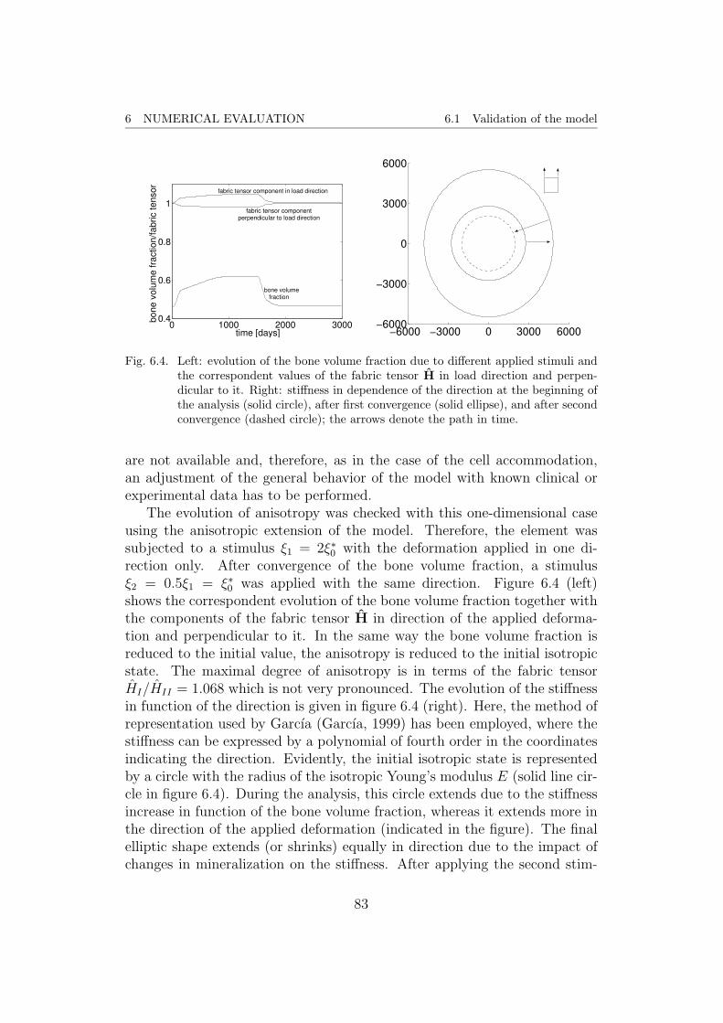
6 NUMERICAL EVALUATION 6.1 Validation of the model
0 1000 2000 30000.4
0.6
0.8
1
time [days]
bone
vol
ume
fract
ion/
fabr
ic te
nsor
bone volumefraction
fabric tensor componentperpendicular to load direction
fabric tensor component in load direction
−6000 −3000 0 3000 6000−6000
−3000
0
3000
6000
Fig. 6.4. Left: evolution of the bone volume fraction due to different applied stimuli andthe correspondent values of the fabric tensor H in load direction and perpen-dicular to it. Right: stiffness in dependence of the direction at the beginning ofthe analysis (solid circle), after first convergence (solid ellipse), and after secondconvergence (dashed circle); the arrows denote the path in time.
are not available and, therefore, as in the case of the cell accommodation,an adjustment of the general behavior of the model with known clinical orexperimental data has to be performed.
The evolution of anisotropy was checked with this one-dimensional caseusing the anisotropic extension of the model. Therefore, the element wassubjected to a stimulus ξ1 = 2ξ∗0 with the deformation applied in one di-rection only. After convergence of the bone volume fraction, a stimulusξ2 = 0.5ξ1 = ξ∗0 was applied with the same direction. Figure 6.4 (left)shows the correspondent evolution of the bone volume fraction together withthe components of the fabric tensor H in direction of the applied deforma-tion and perpendicular to it. In the same way the bone volume fraction isreduced to the initial value, the anisotropy is reduced to the initial isotropicstate. The maximal degree of anisotropy is in terms of the fabric tensorHI/HII = 1.068 which is not very pronounced. The evolution of the stiffnessin function of the direction is given in figure 6.4 (right). Here, the method ofrepresentation used by Garcıa (Garcıa, 1999) has been employed, where thestiffness can be expressed by a polynomial of fourth order in the coordinatesindicating the direction. Evidently, the initial isotropic state is representedby a circle with the radius of the isotropic Young’s modulus E (solid line cir-cle in figure 6.4). During the analysis, this circle extends due to the stiffnessincrease in function of the bone volume fraction, whereas it extends more inthe direction of the applied deformation (indicated in the figure). The finalelliptic shape extends (or shrinks) equally in direction due to the impact ofchanges in mineralization on the stiffness. After applying the second stim-
83

6 NUMERICAL EVALUATION 6.1 Validation of the model
0 500 1000 15000.45
0.5
0.55
0.6
0.65
0.7
time [days]
bone
vol
ume
fract
ion
ω = 0.0ω = 0.1ω = 0.2ω = 0.3
Fig. 6.5. Evolution of the bone volume fraction for different values of ω (left) and theresulting anisotropy in terms of the fabric tensor H. Note the only a quarter ofthe fabric tensor is visualized since it is here double symmetric.
ulus ξ2, the stiffness directionality reduces again to isotropy (in analogy tothe fabric tensor) and results finally in a circle (dashed line circle in figure6.4), which is smaller in radius due to the lower degree of mineralization (cf.results in figure 6.2, where the ash fraction is below its initial value duringthe time of simulation).
The maximal degree of anisotropy in terms of the stiffness is EI/EII =1.141 which is the square of HI/HII , the degree in terms of the materialdistribution. This relation simply results from the fact the material stiffnessis proportional to H4
i , whereas the the remodeling tensor H is related to thesquare root of the fabric tensor H. All these values are close to 1, i.e., closeto isotropy, because the parameter defining the impact of anisotropy of theapplied stimulus tensor Y is small, ω = 0.2. A higher value of ω evidentlyyielded a more pronounced degree of anisotropy. Furthermore, the model isdeveloped in order to simulate changes in anisotropy due to changes in themechanical environment and cannot predict while starting from a fictitioussituation. The direct relation of the evolution of the remodeling tensor Hwith the changes in bone volume fraction vb (cf. equation (5.35)) allowschanges in anisotropy only when the bone volume fraction changes, which isan insufficiency in the formulation of the model.
An variation of the parameter ω which is defining the impact of thedirectionality of the stimulus Y (cf. equation (5.32)) is provided in figure6.5. Obviously, this parameter has a significant influence on the velocity ofconvergence (left). This effect is caused by a change in the scalar stimulus ξwhich is controlling the BMU birthrate. Due to the deviation of the stiffnessin load direction EI from the averaged Young’s modulus E which appears
84

6 NUMERICAL EVALUATION 6.2 THR-prosthesis
in the definition of ξ, the value ξ increases slightly and thereby perturbs theconvergence. In this sense, a higher value ω slows down the convergencebehavior and causes greater changes in bone volume fraction. On the otherhand, this parameter controls the final degree of anisotropy (figure 6.5, right)which can be adjusted to experimental findings.
6.2 THR-prosthesis
A FE model of the proximal femur has been studied extensively in the con-text of computer simulations of bone remodeling. Carter et al. () employeda 2D model with 3 load cases due to the forces in human gait. Their al-gorithm provided creditable results after 300 simulated days while startingfrom a uniform density distribution throughout the whole model. The pre-dicted results are in good consistence with the real structure in a longitudinalsection of the proximal femur. Nevertheless, the algorithm did not producereasonable results in a long-term analysis. In fact, the numerical solutionstarted oscillating and the structural similarities with a real density distri-bution disappeared (Garcıa, 1999, Jacobs, 1994). The same algorithm hasbeen applied to simulate the structural changes after a total hip replacement(THR) with a prosthesis of the type Exeter by Doblare and Garcıa (Garcıa,1999). Although the problem of atrophy in the cortex and the thereby causedreduction in lifetime of the prosthetic device could be predicted, an excessivebone resorption occurred in a longer simulation.
Applying the here proposed method to the same models always resultedin a converging behavior of the numerical outcome, but did not sufficientlyapproach the real density distribution either. But we assume that this iscaused by the unrealistic characteristics of the model. From a biological pointof view, it is impossible to predict the real internal bone structure startingthe simulation with a non-real uniform distribution. The real internal (andexternal) structure of the femur or any other bone is not only a productof mechanical adaptation, but is definitely a result of the combination ofskeletal growth with the impact of mechanical and metabolic factors andinternal remodeling. Therefore, simply taking the outer shape of a femur witha uniform density distribution in its interior cannot result just by internalremodeling in its real structure. Since our purpose is to simulate internalremodeling exclusively, a more reasonable approach is to take the real internaldensity (or bone volume fraction) distribution as initial state and apply themethod. Therefore, we employed the Stanford model () for the first 300 daysin order to predict a reasonable structure and applied our method afterwards.
85
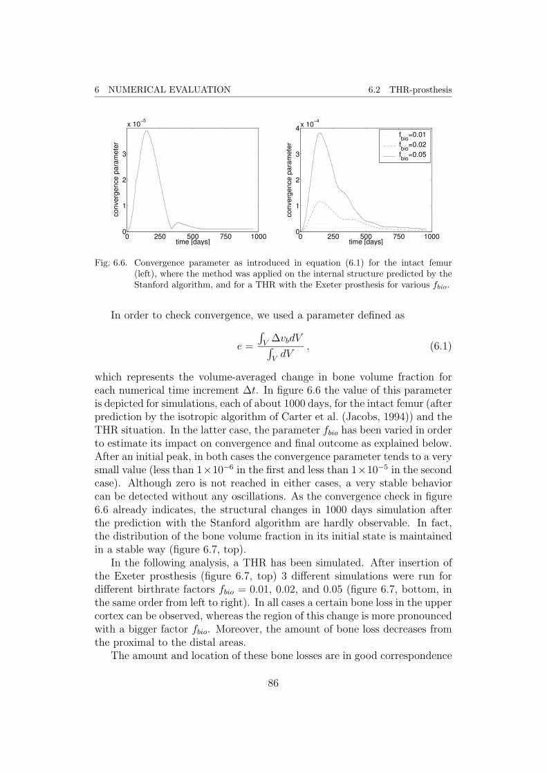
6 NUMERICAL EVALUATION 6.2 THR-prosthesis
0 250 500 750 10000
1
2
3
x 10−5
time [days]
conv
erge
nce
para
met
er
0 250 500 750 10000
1
2
3
4x 10⁻⁴
time [days]
conv
erge
nce
para
met
er
fbio
=0.01fbio
=0.02fbio
=0.05
Fig. 6.6. Convergence parameter as introduced in equation (6.1) for the intact femur(left), where the method was applied on the internal structure predicted by theStanford algorithm, and for a THR with the Exeter prosthesis for various fbio.
In order to check convergence, we used a parameter defined as
e =
∫V
∆vbdV∫VdV
, (6.1)
which represents the volume-averaged change in bone volume fraction foreach numerical time increment ∆t. In figure 6.6 the value of this parameteris depicted for simulations, each of about 1000 days, for the intact femur (afterprediction by the isotropic algorithm of Carter et al. (Jacobs, 1994)) and theTHR situation. In the latter case, the parameter fbio has been varied in orderto estimate its impact on convergence and final outcome as explained below.After an initial peak, in both cases the convergence parameter tends to a verysmall value (less than 1×10⁻⁶ in the first and less than 1×10⁻⁵ in the secondcase). Although zero is not reached in either cases, a very stable behaviorcan be detected without any oscillations. As the convergence check in figure6.6 already indicates, the structural changes in 1000 days simulation afterthe prediction with the Stanford algorithm are hardly observable. In fact,the distribution of the bone volume fraction in its initial state is maintainedin a stable way (figure 6.7, top).
In the following analysis, a THR has been simulated. After insertion ofthe Exeter prosthesis (figure 6.7, top) 3 different simulations were run fordifferent birthrate factors fbio = 0.01, 0.02, and 0.05 (figure 6.7, bottom, inthe same order from left to right). In all cases a certain bone loss in the uppercortex can be observed, whereas the region of this change is more pronouncedwith a bigger factor fbio. Moreover, the amount of bone loss decreases fromthe proximal to the distal areas.
The amount and location of these bone losses are in good correspondence
86

6 NUMERICAL EVALUATION 6.2 THR-prosthesis
Fig. 6.7. Numerical outcome of the proposed method applied on a model of the proxi-mal femur before and after THR. Upper row: the internal density distributionafter 300 simulated days with the Stanford algorithm and 1000 days with thenew model (middle). The initial state directly after the THR-operation (right).Lower row: density distributions 1000 days after THR for the birthrate factor(from left to right) of fbio = 0.01, 0.02, and 0.05.
87

6 NUMERICAL EVALUATION 6.2 THR-prosthesis
Fig. 6.8. Changes in bone area (A) and density (B) due to a THR, taken from Maloneyet al., 2002.
to clinical results (Maloney et al., 2002). As shown in figure 6.8, the meanbone loss observed due to analyses of various patients after a THR in thelateral and medial cortex is of the order of about 20% depending on thesite of measurement. This amount can be well imitated by adjusting theparameters in our model. Furthermore, these structural changes take mainlyplace in the first year after THR in the numerical simulation. A result, whichis confirmed by clinical observations (Maloney et al., 2002).
88

7 OUTLOOK
7 Outlook
In the above, the adaptive character of bone in terms of internal remodel-ing has been presented and, after reviewing several algorithms to performa computer simulation, a new method has been developed, which describesthis process by taking into account microcstructural aspects, such as cellactivity and mineralization, and incorporating a continuum damage modelin consistency with experimental results. Therefore, the history-dependentand coupled events of tissue resorption and formation have been modeled byconsidering the spatial dimension and progression of the relevant cell units(BMU), which are assumed to be activated by a strain-based mechanicalstimulus and microdamage. Furthermore, the anisotropic character of bonehas been expressed by means of the fabric tensor which aligns its principlesaxes with those of the state of deformation. The final constitutive law hasbeen expressed in correlation with experimental findings in terms of the massfraction and distribution of the tissue, its degree of mineralization resultingfrom a time-dependent saturation process, and the current state of dam-age. Parameters have assumed values which were either adjusted —as far aspossible— to known data or estimated reasonably. The whole algorithm wasimplemented as a material subroutine to a finite element software package.Simulating a model of an intact proximal femur and a total hip replacement,has produced creditable results in good consistence with clinical observationsand with an overall converging behavior of the numerical solution.
Currey, 1995, proposed a high standard for bone remodeling algorithmsand it has been a guideline in the development and evaluation of this newmethod. In this sense, some remarks concerning its reliability have to bemade. Generally, the whole model is phenomenological, i.e., it is directlytranslating the observed phenomenon into mathematical expressions. Butthere is a lack of certainty in these observations, most of which are vaguelyquantified and show significant variations. Furthermore, the here used inter-pretation of data is not unique but one out of many reasonable possibilities.Additionally, many assumptions are not verified at all, e.g., the activation ofremodeling in terms of the continuum damage variable.
Although useful results have been produced numerically, the developedalgorithm has not been tested exhaustively. Apart from the many parameterswhich have not been analyzed sufficiently, a huge number of examples —especially in three dimensions— has to be run, controlled and comparedwith clinically given data for a reliable validation.
89

A BASIC CONCEPTS OF CONTINUUM DAMAGE MECHANICS
APPENDIX
As a supplement, some basic ideas of continuum damage mechanics are in-troduced in A, the term fabric tensor as a quantitative description of thedegree of anisotropy is presented in B, the used FE-models are shown in C,and a summary of the algorithms is given in D.
A Basic concepts of continuum damage me-
chanics
Since the appearance and evolution of microdamage plays an important rolein the context of bone remodeling, some basic items of damage mechanicswill be presented. In Ibijola, 2002, Lemaitre, 1985, and Simo and Ju, 1987,more details on continuum damage mechanics in general can be found. Acertain damage model for bone is given in Garcıa, 1999, and the subsequentpublication, Doblare and Garcıa, 2002, which is mathematically based in thedescription of anisotropy due to damage by Cordebois and Sidoroff, 1982.Dwight and Jepsen, 2001, list various approaches to describe bone damage.
For sake of simplicity, a few assumptions have to be made: strains anddisplacements are to be small, thermal and plasticity effects will be neglected.The results of this appendix refer to inert materials, i.e., materials which donot have the capability to repair themselves.
Damage is usually described by an independent variable D which is atensor and reduces to the scalar d in the isotropic case. This variable D con-tains the necessary information about the damage state in the given materialpoint, i.e., it is a measure for the number and size (and orientation, in theanisotropic case) of defects.
First, the isotropic case will be discussed. Therefore, only the scalar d isneeded to describe the degree of damage. d has typically a range from 0 to1, where d = 0 corresponds to the undamaged (virgin) material and d = 1generally presents the rupture of the given element.
A necessary tool is the concept of effective stress . It describes the imagi-nary stress field σ which yielded the same strains in an undamaged materialas does the real stress σ in the damaged material. Effective and real stressare related by
σ =σ
1− d. (A.1)
Taking now the constitutive equation σ = C0 : ε, where C0 refers to thestiffness of the undamaged material, one can easily get the stress-strain re-lation for damage mechanics, since the real and imaginary (caused by the
90

A BASIC CONCEPTS OF CONTINUUM DAMAGE MECHANICS
effective stress) strains have been assumed to be equal,
σ = (1− d)C0 : ε = C : ε (A.2)
with C being the current stiffness tensor, a function of d.Additionally, some comments on the thermodynamics of this process have
to be made. Since thermal and plasticity effects are excluded, this will beconcentrated on the elastic part of the free energy function ψel(ε, D), whichis defined as
ψel =1
2ε : C : ε . (A.3)
ψel is also referred to as the elastic potential and its existence classifies thematerial to be hyperelastic. Although already employed, the stress tensorcan now be defined as
σ =∂ψel
∂ε= C : ε = (1− d)C0 : ε (A.4)
evidently yielding the same relation as in (A.2).But the elastic potential depends as well on the damage variable d and
in the same manner an associated variable is constructed
Yd =∂ψel
∂d= −1
2ε : C0 : ε . (A.5)
Obviously, −Yd = ψel0 with ψel0 being the free energy in the undamaged state(d = 0).
The second law of thermodynamics imposes a restriction on dissipationwhich can be represented in terms of the Clausius-Duhem inequality
−ψ + σ : ε ≥ 0 . (A.6)
Taking into account that ψ = ψel and applying relations (A.2) and (A.5),equation (A.6) can be formulated as
−Ydd = ψel0 d ≥ 0 . (A.7)
ψel is always positive (cf. its definition in (A.3)) and, therefore, the damagerate d has to be positive or zero. This is a fairly logic result, since damagecan only increase. Note, that this conclusion does not hold for bone. Boneis not inert but a living tissue and possesses the capability to repair damage.
In an anisotropic case, as it will be used for the method of Garcıa andDoblare (cf. Garcıa, 1999, and Doblare and Garcıa, 2002) and the new model,where porosity is interpreted as anisotropic damage, the damage state has
91

A BASIC CONCEPTS OF CONTINUUM DAMAGE MECHANICS
to be represented by a tensor quantity. In general, a fourth-order tensor isneeded for a full description of the problem, but here the material is assumedto be locally orthotropic such that D will be a symmetric second-order tensor.From the variety of formulations of the effective stress (cf. Cordebois andSidoroff, 1982) one expression is chosen
σ = (1−D)1/2 : σ : (1−D)1/2 , (A.8)
which conserves the symmetry of stresses. The thermodynamic restriction isequivalently
−YD : D ≥ 0 (A.9)
where the associated variable YD is defined as on the left side of expression(A.5). In Cordebois and Sidoroff, 1982, the constitutive relation in principalaxes of D is derived. The final result in form of the components of thecompliance tensor F = C−1 is then
1
EI=
1
E
1
(1−DI)2
−νI IIEII
= −νII IEI
= − νE
1
(1−DI)(1−DII)
1
2GI II
=1 + ν
E
1
(1−DI)(1−DII)
(A.10)
where the other components are given by mutual rotation of the indices I,II, and III. The parameters E and ν refer to the Young’s modulus andPoisson’s ration of the undamaged material.
92

B FABRIC TENSOR
Fig. B.1. Left: example to determine the mean intercept length in a given bone specimen.Right: mean intercept length as a function of the angle θ. Taken from Martinet al., 1998.
B Fabric tensor
In the following, the geometric quantity fabric tensor will presented. A moreprecise analysis can be found in Cowin, 1986.
Although in some methods treated like a homogeneous isotropic mate-rial, bone tissue shows different properties in reality. It is actually a porousinhomogeneous anisotropic structure. Hence, a more precise description ofthe mechanical behavior of this tissue requires accounting for its structuralanisotropy. Bone stereology provides the adequate means for measuring thedegree of this feature.
Superimposing test lines oriented at a certain angle θ with respect to areference line allows to measure the mean intercept length L, which is theaverage distance between two bone-marrow interfaces. Obviously, the meanintercept length is a function of the orientation of the used test lines, i.e.,L = L(θ). It has been shown that plots of L in a polar diagram produceellipses and, moreover, data fit closely the equation
1
L2(θ)= M11 cos2 θ + 2M12 sin θ cos θ +M22 sin2 θ . (B.1)
In figure B.1, an example for measurement of the mean intercept length andits presentation in a diagram is given.
Furthermore, varying the direction n of the test lines through all threedimensions yields the ideal extension that the values of the mean interceptlength can be approximately represented by an ellipsoid. Therefore, a second-order tensor M can be introduced such that the following relation holds
1
L2(n)= nTMn . (B.2)
93

B FABRIC TENSOR
Finally, the quantity representing the structural anisotropy of cancellous bonewill be the fabric tensor defined as
H = M−1/2 . (B.3)
Definition (B.3) is not problematic, since the mean intercept length tensorM is symmetric and positive definite. This property follows directly fromthe fact, that M can be geometrically represented by an ellipsoid. In anisotropic situation, the fabric tensor H will evidently be the multiple of theidentity tensor I, in detail H = l I with l the mean intercept length, nowbeing constant in all directions.
Additionally, one statement of Wollf’s law (alignment of the trabeculaewith the principal stress trajectories) can be represented by the followingresults
T∗H∗ = H∗T∗ and E∗H∗ = H∗E∗ , (B.4)
where the asterisk indicates that the quantity is in remodeling equilibrium.The derivation of equations (B.4) is given in Cowin, 1986.
94
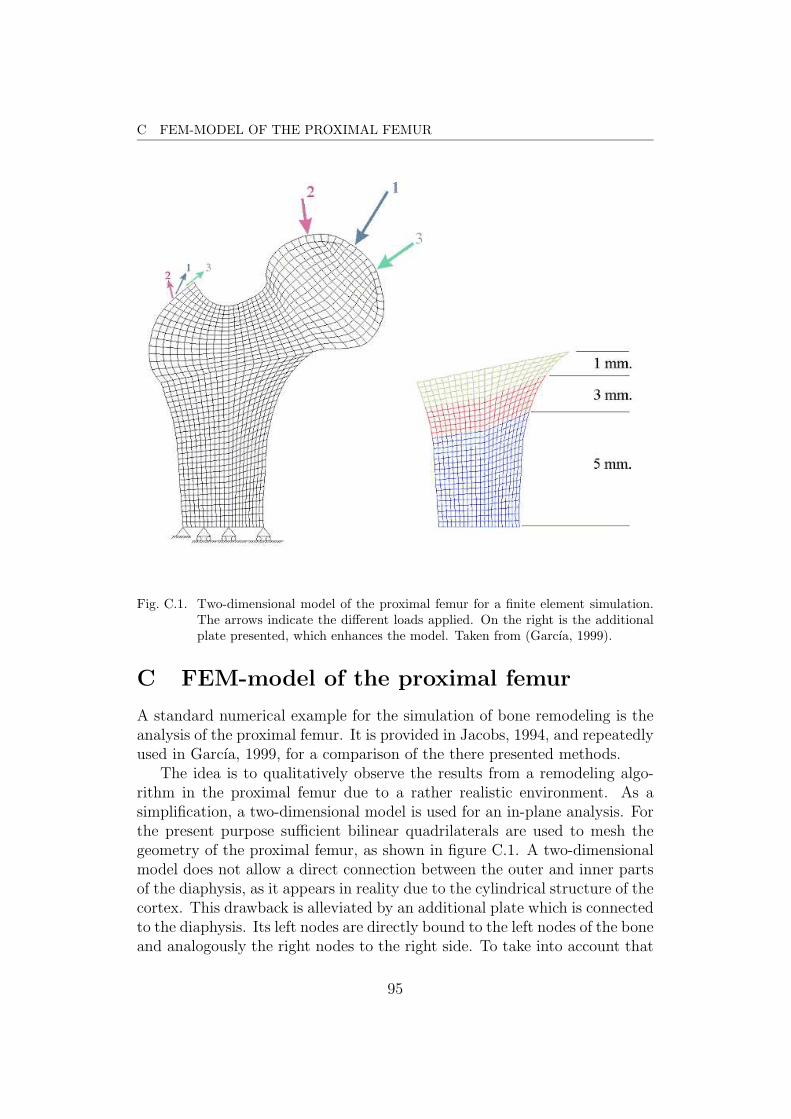
C FEM-MODEL OF THE PROXIMAL FEMUR
Fig. C.1. Two-dimensional model of the proximal femur for a finite element simulation.The arrows indicate the different loads applied. On the right is the additionalplate presented, which enhances the model. Taken from (Garcıa, 1999).
C FEM-model of the proximal femur
A standard numerical example for the simulation of bone remodeling is theanalysis of the proximal femur. It is provided in Jacobs, 1994, and repeatedlyused in Garcıa, 1999, for a comparison of the there presented methods.
The idea is to qualitatively observe the results from a remodeling algo-rithm in the proximal femur due to a rather realistic environment. As asimplification, a two-dimensional model is used for an in-plane analysis. Forthe present purpose sufficient bilinear quadrilaterals are used to mesh thegeometry of the proximal femur, as shown in figure C.1. A two-dimensionalmodel does not allow a direct connection between the outer and inner partsof the diaphysis, as it appears in reality due to the cylindrical structure of thecortex. This drawback is alleviated by an additional plate which is connectedto the diaphysis. Its left nodes are directly bound to the left nodes of the boneand analogously the right nodes to the right side. To take into account that
95
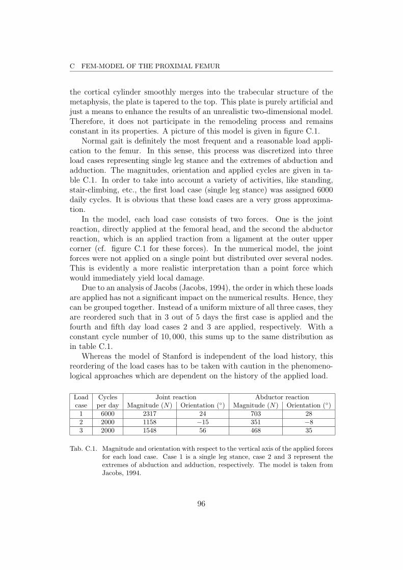
C FEM-MODEL OF THE PROXIMAL FEMUR
the cortical cylinder smoothly merges into the trabecular structure of themetaphysis, the plate is tapered to the top. This plate is purely artificial andjust a means to enhance the results of an unrealistic two-dimensional model.Therefore, it does not participate in the remodeling process and remainsconstant in its properties. A picture of this model is given in figure C.1.
Normal gait is definitely the most frequent and a reasonable load appli-cation to the femur. In this sense, this process was discretized into threeload cases representing single leg stance and the extremes of abduction andadduction. The magnitudes, orientation and applied cycles are given in ta-ble C.1. In order to take into account a variety of activities, like standing,stair-climbing, etc., the first load case (single leg stance) was assigned 6000daily cycles. It is obvious that these load cases are a very gross approxima-tion.
In the model, each load case consists of two forces. One is the jointreaction, directly applied at the femoral head, and the second the abductorreaction, which is an applied traction from a ligament at the outer uppercorner (cf. figure C.1 for these forces). In the numerical model, the jointforces were not applied on a single point but distributed over several nodes.This is evidently a more realistic interpretation than a point force whichwould immediately yield local damage.
Due to an analysis of Jacobs (Jacobs, 1994), the order in which these loadsare applied has not a significant impact on the numerical results. Hence, theycan be grouped together. Instead of a uniform mixture of all three cases, theyare reordered such that in 3 out of 5 days the first case is applied and thefourth and fifth day load cases 2 and 3 are applied, respectively. With aconstant cycle number of 10, 000, this sums up to the same distribution asin table C.1.
Whereas the model of Stanford is independent of the load history, thisreordering of the load cases has to be taken with caution in the phenomeno-logical approaches which are dependent on the history of the applied load.
Load Cycles Joint reaction Abductor reactioncase per day Magnitude (N) Orientation () Magnitude (N) Orientation ()
1 6000 2317 24 703 282 2000 1158 −15 351 −83 2000 1548 56 468 35
Tab. C.1. Magnitude and orientation with respect to the vertical axis of the applied forcesfor each load case. Case 1 is a single leg stance, case 2 and 3 represent theextremes of abduction and adduction, respectively. The model is taken fromJacobs, 1994.
96

C FEM-MODEL OF THE PROXIMAL FEMUR
Fig. C.2. From left to right: A schematic drawing of the Exeter prosthesis, the finiteelement mesh with sideplate, and the application of the loads after insertion ofthe prosthesis.
A second model of application is the proximal femur with a total hipreplacement prosthesis. In cases of a fracture in the femoral head or neck,fixations or prosthetic devices have to be used in order to cure the problem.Whereas in the former case metal struts attached with screws or nails helpto fixate the fractured parts, in the case of a total hip replacement the fulljoint is replaced by a prosthesis. Here, the femoral head is cut off and theprosthesis is cemented into the proximal femur. Such a prosthesis, the modelExeter , can be seen in figure C.2.
On the left, a drawing of such a prosthesis is given. The cement is pre-sented in blue and the polymeric counterpart in the pelvis is white. In themiddle, the used meshes are presented. One can see the different parts rep-resenting in total the femur before the operation. Afterwards, the femoralhead is removed(cyan), and the prosthesis (green) is inserted with the ce-ment (yellow). The side plate is equivalent to the one used in the previousmodel without prosthesis. The loads are applied in with same direction andmagnitude as in the normal model. Before the operation they are applied onthe femoral head as in figure C.1 and afterward on the head of the prosthesisas shown in the picture on the right.
97
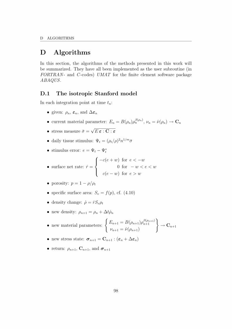
D ALGORITHMS
D Algorithms
In this section, the algorithms of the methods presented in this work willbe summarized. They have all been implemented as the user subroutine (inFORTRAN - and C -codes) UMAT for the finite element software packageABAQUS .
D.1 The isotropic Stanford model
In each integration point at time tn:
• given: ρn, εn, and ∆εn
• current material parameter: En = B(ρn)ρβ(ρn)n , νn = ν(ρn) → Cn
• stress measure σ =√E ε : C : ε
• daily tissue stimulus: Ψt = (ρt/ρ)2n1/mσ
• stimulus error: e = Ψt −Ψ∗t
• surface net rate: r =
−c(e+ w) for e < −w
0 for − w < e < w
c(e− w) for e > w
• porosity: p = 1− ρ/ρt
• specific surface area: Sv = f(p), cf. (4.10)
• density change: ρ = rSvρt
• new density: ρn+1 = ρn + ∆tρn
• new material parameters:
En+1 = B(ρn+1)ρ
β(ρn+1)n+1
νn+1 = ν(ρn+1)
→ Cn+1
• new stress state: σn+1 = Cn+1 : (εn + ∆εn)
• return: ρn+1, Cn+1, and σn+1
98

D ALGORITHMS D.2 The energy-based anisotropic extension by Jacobs
D.2 The energy-based anisotropic extension by Jacobs
In each integration point at time tn:
• given: ρn, εn, ∆εn, σn, and Cn
• remodeling criteria: f j(ε,C, ρ) due to equation (4.28)
• If f r ≥ 0 and f f < 0 resorption: ρ = −c fr
ρ2−β/2Sv
• If f r < 0 and f f < 0 dead zone: ρ = 0 and C = 0
• If f r < 0 and f f ≥ 0 formation: ρ = c ff
ρ2−β/2Sv
• new density: ρn+1 = ρn + ∆tρn
• in resorption: F = βρρε⊗εσ:ε
Fn+1 = Fn + ∆tFn → Cn+1 = F−1n+1
• in formation: C = βρρσ⊗σσ:ε→ Cn+1 = Cn + ∆tCn
• new stress state: σn+1 = Cn+1 : (εn + ∆εn)
• return: ρn+1, Cn+1, and σn+1
D.3 The damage-based model by Garcıa and Doblare
• given: εn, ∆εn, σn, and Hn
• current compliance tensor: Fn = f(Hn), cf. equation (4.33)
• energy associated variable:
Yn = 2(λ tr(H2
nεn)Hnεn + 2µ(HnεnHn)(Hnεn))
• the stimulus tensor: Jn = 13(1− 2ω) tr(Y)1 + ωY
• remodeling criteria: gj(J, ρ, ω) due to equations (4.38).
• If gr ≥ 0 and gf < 0 resorption: H = f(J,H, ρ, ω), equation (4.39)
• If gr < 0 and gf < 0 dead zone: H = 0
• If gr < 0 and gf ≥ 0 formation: H = f(J,H, ρ, ω)
• new remodeling tensor: Hn+1 = Hn + ∆tHn
99

D ALGORITHMS D.4 The method of Hazelwood, Martin, et al.
• new density: ρn+1 =(
det(H2n+1)
A3/2
)2/(3β)
ρt
• new compliance tensor: Fn+1 = f(Hn+1), cf. equation (4.33)
• inversion yields new stiffness tensor: Cn+1 = F−1n+1
• new stress state: σn+1 = Cn+1 : (εn + ∆εn)
• return: Hn+1, Cn+1, and σn+1
D.4 The method of Hazelwood, Martin, et al.
• given: εn, pn, Dn, ∆εn, and the array of the past activation frequenciesfa[ ] with the latest value fa,n
• principle (compressive) strain: ε
• stimulus: Φ = Nε q
• mechanical damage growth rate: DM = kDΦ
• damage removal rate due to remodeling: DR = Dnfa,nAFs
• damage rate: D = DM − DR
• new damage state: Dn+1 = Dn + D∆t
• activation due to damage: fa,dam = f(D)
• IF Φ < Φ0 disuse: activation due to disuse fa,dis = f(Φ)reduced area for formation A = A(0.5 + 0.5Φ/Φo)
• normalized specific surface area: Sv = f(p)
• new activation frequency: fa,n+1 = Sv(fa,dam + fa,dis)
• update frequency array fa[ ]: fa[i] = fa[i− 1] and fa[0] = fa,n+1
• BMU density for resorption: NR =∫ tt−TR
fa(t′)dt′
• BMU density for formation: NR =∫ t−TR−TIt−TR−TI−TF
fa(t′)dt′
• porosity rate of change: p = NRQR −NFQF
• new porosity: pn+1 = pn + p∆t
100

D ALGORITHMS D.5 A new approach
• new Young’s modulus: En+1 = f(pn+1)→ Cn+1
• new stress state: σn+1 = Cn+1 : (εn + ∆εn)
• return: pn+1, Dn+1, σn+1, Cn+1, and store updated frequency arrayfa[ ]
D.5 A new approach
• given: Hn, vb,n, αn, dn, εn, ∆εn,and the array of recent BMU-birhtrates NBMU
• calculate stimuli ξ and Y
• received level of inhibitory signal: s = f(ξ, d)
• origination frequency: for = fbio(1− s)
• specific surface area: Sv = f(p) with p = 1− vb
• BMU birthrate: NBMU,n+1 = Svfor
• remodeling criteria: gj = f(J) with J the anisotropic stimulus
• focal bone balance: (fb/fc)
• resorption increment: ∆vR by integrating over the history of NBMU
• formation increment: ∆vF analogously
• new bone volume fraction: vb,n+1 = vb,n + ∆vF −∆vR
• update birthrate storage: NBMU [ ]: NBMU [i] = NBMU [i− 1]and NBMU [0] = NBMU,n+1
• new degree of mineralization: αn+1 = f(αn,∆vR,∆vF
• new state of damage: dn+1 = f(dn, ε,∆vR,∆vF , d) with d = vbd
• increment of remodeling tensor: H = f(H,J, vb)
• new remodeling tensor: Hn+1 = Hn + H∆t
• new stiffness tensor: Cn+1 = f(Hn+1, αn+1, dn+1)
• new stress state: σn+1 = Cn+1 : (εn + ∆εn)
• return: vb,n+1, αn+1, dn+1, Hn+1, σn+1, Cn+1,and store updated birthrate array NBMU [ ]
101

LIST OF FIGURES LIST OF FIGURES
List of Figures
2.1 Human skeleton and a long bone . . . . . . . . . . . . . . . . 42.2 Trabecular and cortical bone . . . . . . . . . . . . . . . . . . . 72.3 Cortical bone structure . . . . . . . . . . . . . . . . . . . . . . 82.4 Mineralization process . . . . . . . . . . . . . . . . . . . . . . 122.5 Different models for the E-Modulus . . . . . . . . . . . . . . . 142.6 Damage evolution . . . . . . . . . . . . . . . . . . . . . . . . . 173.1 Fairbairne crane and proximal femur . . . . . . . . . . . . . . 193.2 Cortical and cancellous BMUs . . . . . . . . . . . . . . . . . . 233.3 Remodeled volume unit . . . . . . . . . . . . . . . . . . . . . . 244.1 Daily stimulus . . . . . . . . . . . . . . . . . . . . . . . . . . . 304.2 Specific surface area and rate relationships . . . . . . . . . . . 334.3 Stanford algorithm . . . . . . . . . . . . . . . . . . . . . . . . 354.4 Results of the Stanford model . . . . . . . . . . . . . . . . . . 364.5 Convergence analysis of the Stanford model . . . . . . . . . . 374.6 Anisotropy of the methods of Jacobs and of Garcıa and Doblare 454.7 Activation frequency in response to disuse and damage . . . . 504.8 Algorithm for the method of Hazelwood et al. . . . . . . . . . 514.9 Porosity evolution in the model of Hazelwood et. al . . . . . . 524.10 Application of the method of Hazelwood et al. on the proximal
femur model . . . . . . . . . . . . . . . . . . . . . . . . . . . . 544.11 BMU-progression model . . . . . . . . . . . . . . . . . . . . . 555.1 Block diagram of the new model . . . . . . . . . . . . . . . . . 605.2 Cortical and cancellous BMUs . . . . . . . . . . . . . . . . . . 635.3 Volume models . . . . . . . . . . . . . . . . . . . . . . . . . . 665.4 Model for signal function s . . . . . . . . . . . . . . . . . . . . 685.5 Bone focal balance . . . . . . . . . . . . . . . . . . . . . . . . 705.6 Ash fraction during primary and secondary mineralization phases 715.7 Qualitative shape of damage evolution . . . . . . . . . . . . . 736.1 Evolution of bone volume fraction, resorption and formation
increments . . . . . . . . . . . . . . . . . . . . . . . . . . . . . 806.2 Ash fraction and accommodation of the reference stimulus . . 816.3 Bone volume fraction due to differnet focal bone balances and
different biological factors . . . . . . . . . . . . . . . . . . . . 826.4 Fabric tensor components and bone volume fraction and the
anisotropic evolution of the stiffness . . . . . . . . . . . . . . . 836.5 Variation of anisotropy parameter . . . . . . . . . . . . . . . . 846.6 Convergence parameter after Stanford model and after inser-
tion of prosthesis . . . . . . . . . . . . . . . . . . . . . . . . . 86
102
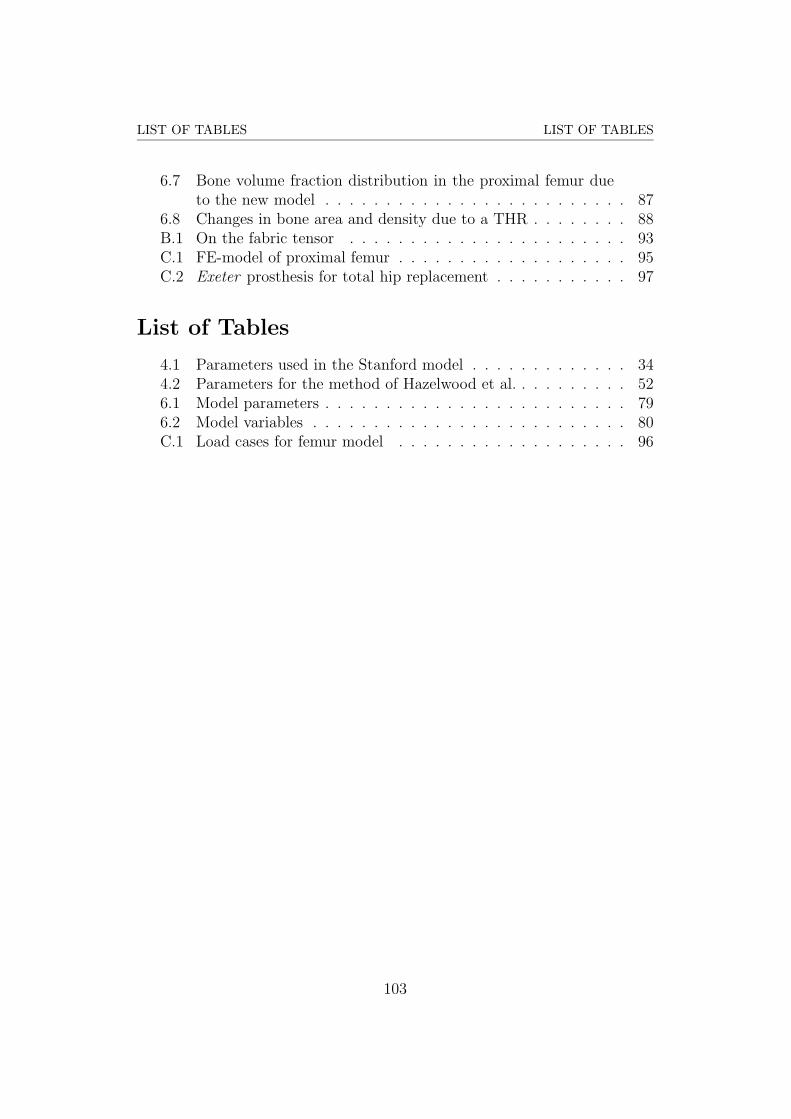
LIST OF TABLES LIST OF TABLES
6.7 Bone volume fraction distribution in the proximal femur dueto the new model . . . . . . . . . . . . . . . . . . . . . . . . . 87
6.8 Changes in bone area and density due to a THR . . . . . . . . 88B.1 On the fabric tensor . . . . . . . . . . . . . . . . . . . . . . . 93C.1 FE-model of proximal femur . . . . . . . . . . . . . . . . . . . 95C.2 Exeter prosthesis for total hip replacement . . . . . . . . . . . 97
List of Tables
4.1 Parameters used in the Stanford model . . . . . . . . . . . . . 344.2 Parameters for the method of Hazelwood et al. . . . . . . . . . 526.1 Model parameters . . . . . . . . . . . . . . . . . . . . . . . . . 796.2 Model variables . . . . . . . . . . . . . . . . . . . . . . . . . . 80C.1 Load cases for femur model . . . . . . . . . . . . . . . . . . . 96
103
REFERENCES REFERENCES
References
Buckwalter JA, Glimcher MJ, Cooper RR, Recker R; 1995.Bone Biology, Part I and Part II. The Journal of Bone and Joint Surgery,Vol. 77-A, No. 8, pp 1255–90.
Carter DR, Beaupre GS; 2001.Skeletal function and form: Mechanobiology of Skeletal Development, Agingand Regeneration; 1st edition. Cambridge University Press, Cambridge.
Cordebois JP, Sidoroff F; 1982.Damage Induced Elastic Anisotropy. Colloques internationaux du CNRS,No. 295, Comportement mecanique des solides anisotropes, pp 761–74.
Cowin SC; 1986.Wolff’s Law of Trabecular Architecture at Remodeling Equilibrium. Journalof Biomechanical Engineering, Vol. 108, pp 83–88.
Currey JD; 1995.The validation of algorithms used to explain adaptive remodeling in bone.From: Bone Structure and Remodeling. Odgaard A, Weinans H (editors).World Scientific, Singapore, pp 9–13
Doblare M, Garcıa JM; 2002.Anisotropic bone remodelling model based on a continuum damage-repairtheory. Journal of Biomechanics, Vol. 35, pp 1–17.
Dwight TD, Jepsen KJ; 2001.Bone Damage Mechanics. Chapter 18 in: Bone Mechanics Handbook; 2ndedition. Cowin SC (editor), CRC Press, pp 18-1–18-25.
Firoozbakhsh K, Aleyaasin M; 1989.The effect of Stress Concentration on Bone Remodeling: Theoretical Predic-tions. Journal of Biomechanical Engineering, Vol. 111, pp. 355–60.
Frost HM; 1983.Bone histomorphometry: Analysis of trabecular bone dynamics. Chapter 7in: Bone Histomorphometry: Techniques and Interpretation. Recker RR, Ra-ton B (editors), CRC Press, pp 109–131.
Fyhrie DP, Schaffler MB; 1995.The adaption of bone apparent density to applied load. Journal of Biome-chanics, Vol. 28, No. 2, pp 135–46.
Garcıa JM; 1999.Modelos de remodelacion osea: Analisis numerico y aplicaciones al diseno defijaciones de fracturas del femur proximal. Tesis Doctoral, Centro PolitecnicoSuperior Zaragoza.
104
REFERENCES REFERENCES
Hazelwood SJ, Martin RB, Rashid MM, Rodrigo JJ; 2001.A mechanistic model for internal bone remodeling exhibits different dy-namic responses in disuse and overload. Journal of Biomechanics, Vol. 34,pp 299–308.
Hernandez CJ, Hazelwood SJ, Martin RB; 1999.The Relationship Between Basic Multicellular Unit Activation and Origina-tion in Cancellous Bone. Bone, Vol. 25, No. 5, pp 585–7.
Hernandez CJ, Beaupre GS, Carter DR; 2001.A model of mechanobiologic and metabolic influences on bone adaption.Journal of Rehabilitation Research and Development, Vol. 37, No. 2,http://www.vard.org/jour/.
Hernandez CJ; 2001.Simulation of bone remodeling during the development and treatment of os-teoporosis. PhD Thesis, Stanford University.
Hernandez CJ, Beaupre GS, Keller TS, Carter DR; 2001a.The influence of Bone Volume Fraction and Ash Fraction on Bone Strengthand Modulus. Bone, Vol. 29, No. 1, pp 74–8.
Hernandez CJ, Beaupre GS, Marcus R, Carter DR; 2001b.A Theoretical Analysis of the Contributions of Remodeling Space, Miner-alization, and Bone Balance to Changes in Bone Mineral Density DuringAlendronate Treatment. Bone, Vol. 29, No. 6, pp 511–16.
Hernandez CJ, Beaupre GS, Carter DR; 2003.A theoretical analysis of the changes in basic multicellular unit activity atmenopause. Bone, Vol. 32, 357–63.
Ibijola EA; 2002.On some fundamental concepts of Continuum Damage Mechanics. Computermethods in applied mechanics and engineering. Vol. 191, pp 1505–20.
Jacobs CR; 1994.Numerical simulation of bone adaption to mechanical loading. PhD Thesis,Stanford University.
Jepsen KJ, Dwight TD, Ozan A; 2001.Observation of Damage in Bone. Chapter 17 in: Bone Mechanics Handbook;2nd edition. Cowin SC (editor), CRC Press, pp 17-1–17-8.
Lemaitre J; 1985.A Continuous Damage Mechanics Model for Ductile Fracture. Journal of En-gineering Materials and Technology, Transactions of the ASME, Vol. 107,pp 83–9.
105

REFERENCES REFERENCES
Maloney WJ, Schmalzried T, Harris WH.Analysis of Long-Term Cemented Total Hip Arthoplasty Retrievals. ClinicalOrthopaedics and Related Research. Vol. 405, pp 70–8.
Martin RB; 1984.Porosity and specific surface of bone. Chapter 3 in: Critical Reviews inBiomedical Engineering, Vol. 10. CRC Press, pp 179-222.
Martin RB, Burr DR, Sharkey NA; 1998.Skeletal Tissue Mechanics. Springer, New York.
Martin RB; 2000.Toward a Unifying Theory of Bone Remodeling. Bone, Vol. 26, No. 1, pp 1–6.
Martin RB; 2002.Is All Cortical Bone Remodeling Initiated by Microdamage? Bone, Vol. 30,No. 1, pp 8–13.
Martin RB; 2003.Fatigue Damage, Remodeling, and the Minimization of Skeletal Weight. Jour-nal of theoretical Biology, Vol. 220, pp 271–6.
Mullender MG, Huiskes R, Weinans H; 1994.A physioligical approach to the simulation of bone remodeling as a self-organizational control process. Journal of Biomechanics, Vol. 27, No. 11,pp 1389–94.
Ogden RW; 1984.Non-linear elastic deformations. Dover Publications, Mineola, New York.
Parfitt AM, Drezner MK, Glorieux FH, Kanis JA, Malluche H, Meunier PJ, OttSM, Recker RR; 1987.
Bone Histomorphometry: Standardization of Nomenclature, Symbols, andUnits. Journal of Bone and Mineral Research, Vol. 2, No. 6, pp 595–610.
Parfitt AM; 1994.Osteonal and Hemi-Osteonal Remodeling: The Spatial and Temporal Frame-work for Signal Traffic in Adult Human Bone. Journal of Cellular Biochem-istry, Vol. 55, pp 273–86.
Parfitt AM; 2002.Targeted and Nontargeted Bone Remodeling: Relationship to Basic Multicel-lular Unit Origination and Progression. Bone, Vol. 30, No. 1, pp 5–7.
Pattin CA, Caler WE, Carter DR; 1996.Cyclic mechanical property degradation during fatigue loading of corticalbone. Journal of Biomechanics, Vol. 29, No. 1, pp 69–79.
106

REFERENCES REFERENCES
Peerlings RHJ; 1999.Enhanced damage modelling for fracture and fatigue. PhD Thesis, TechnischeUniversiteit Eindhoven.
Ramtani S, Zidi M; 2001.A theoretical model of the effect of continuum damage on a bone adaptionmodel. Journal of Biomechanics, Vol. 34, pp 471–79.
Rubin C, Turner AS, Bain S, Mallinkrodt C, McLeod K; 2001.Low mechanical signals strengthen long bones. Nature, Vol. 412, pp 603–4.
Simo JC, Ju JW; 1987.Strain- and stress-based continuum damage models—I. formulation. Interna-tional Journal of Solids and Structures, Vol. 23, No. 7, pp 821–40.
Stulpner MA, Reddy BD, Starke GR, Spirakis A; 1997.A three-dimensional finite analysis of adaptive remodelling in the proximalfemur. Journal of Biomechanics, Vol. 30, No. 10, pp 1063–7.
Turner CH; 1999.Toward a Mathematical Description of Bone Biology: The Principle of Cel-lular Accommodation. Calcified Tissue International, Vol. 65, pp 466–71.
van der Meulen MCH, Huiskes R; 2002.Why mechanobiology? A survey article. Journal of Biomechanics, Vol. 35,pp 401–14.
Vico L, Collet P, Guignandon A, Lafage-Proust M-H, Thomas T, Rehailia M,Alexandre C; 2000.
Effects of long-term microgravity exposure on cancellous and cortical weight-bearing bones of cosmonauts. The Lancet, Vol. 355, pp 1607–11.
Zhu X, Gong H, Zhu D, Gao B; 2002.A study of the effect of non-linearities in the equation of bone remodeling.Journal of Biomechanics, Vol. 35, pp 951–60.
Zioupos P, Casinos A; 1998.Cumulative damage and the response of human bone in two-step loadingfatigue. Journal of Biomechanics, Vol. 31, pp 825–33.
107