MEMORANDUM

RM-5883-PRJANUARY 1W69

0DIGITAL COMPUTER SIMULATION:

COMPUTER PROGRAMMING LANGUAGES

Philip J. Kiviat

DDC

VAR 2116

PREPARED FOR:

UNITED STATES AIR FORCE PROJECT RAND

SANIA MONIC.A * (.ALIFORiNIA-

_ - _ _ __,_ _

llllriu,,.

MEMORANDUM

RM-5883-PRJANUARY 1969

DIGITAL COMPUTER SIMULATION:

COMPUTER PROGRAMMING LANGUAGESPhilip J. Kiviat

This, research is support.,iI by the United States Air Force under Projet RANfD-Con.tract No. F4 1620-67-C-0015- monitored by the Directora le of Operalional |equiremeintsand Development Plans. l)eputl Chief of Staff. Research and I)evelolmtent. l1 USAF.Views or -conclusion. conhin(l in thi-t study should not I.e interpreted as repre.ntingthe official opinion or poli,'y of the Urnized State, Air Force.

DISTRIBUTION STATEMENTThis document has been approved for public releaw and sale; its distribhulion is unlimited.

PREFACE

This RAND Memorandum is one in a continuing series on the tech-

niques of digital computer simulation. Each Memorandum covers a

selected topic or subject area in considerable detail. This study

discusses computer simulation programming languages. It describes

their characteristics, considers reasons for using them, compares their

advantages and disadvantages relative to other kinds of programming

languages and, through examples, compares four of the most popular

simulation languages in use today.

The Memoranda are being written so that they build upon one another

and provide an integrated coverage of all aspects of simulation. The

only Hemorandum in the series that needs to be read before this one is

P. J. Kiviat, Digital Computer Simulation: Modeling Concepts, The

RAND Corporation, RM-5378-PR, August 1967. All the Memoranda should

be of particular interest to personnel of the AFLC Advanced Logistics

System Center, Wright-Patterson Air Force Base, and to Air Force sys-

tems analysts and computer programmers. Persons responsible for

selecting simulation programming languages for particular projects or

for installations of computer systems should find this Memorandum

particularly useful.

-v -

S IJMARY

Simulation programming languages are designed to assist analysts

in the design, programming, and analysis of simulation models. This

Memorandum discusses basic simulation concepts, presents arguments for

the'use of simulation languages, discusses the four languages GPSS,

SIMSCRIPT II, SIMUIA, and CSL, suammrizes their basic features, and

con nents on the probable future course of events in simulation inguage

research and development.

Simulation languages are shown to assist in the design of simula-

tion models through their "world view," to expedite computer programming

through their special purpose, high-level statements, and to encourage

proper model analysis through their data collection, analysis, and

reporting features. Ten particularly important simulation programming

language features are identified: modeling a system's static state,

modeling system dynamics, statistical sampling, data collection, analysis

and display, monitoring and debugging, initialization and language

usability. Examples of each of the four simulation languages, GPSS,

SIMSCRIPT II, SIMULA, and CSL, are used to illustrate how these features

are implemented in different languages.

The future development of simulation programming languages is

shown to be dependent on advances in the fields of computer languages,

computer graphics, and time sharing. Some current research is noted;

outstanding research areas are identified.

Y=

(F. -vii-

CONTENTS

IPREFACE . i

SU ?' 4RY ......................................................... v

SeCgion.I, INTRODUCTION . ......................... ................. I

Some Definitions ........................................ IPrincipal Features of Simulation Languages .............. 4Reasons for Having SPLs ................................. 6Reasons for Using Existing POLs ......................... 7

II. SIMULATION PROGRAMMING CONCEPTS ........................... 10Describing a System: The Static Structure .............. 10Describing a System: The Dynamic Structure ............. 14

III. SIMULATION PROGRAMMINC LAI.GUAGE FEA 'JRES .................. 26Specifying System Structure ............................. 26Representing Statistical Phenomena ...................... 26Data Collection, Analysis, and Display .................. 30Monitoring and Debugging ................................ 35

Initialization . .......................................... 36Other Features . .......................................... 37

IV. SOME EXAIPLES OF SPLS . ..................................... 39SIMSCRIPT II; An Eveat-Oriented Language ............... 39SIMULA: A Process-Oriented Language .................... 63

CSL: An Activity-Oriented Language ..................... 75GPSS/360: A Transaction-Flow Languige .................. 85SUMMARY . ................................................. 90

V. CURRENT SPL RESFARCH ....................................... 91Research on Simulation concepts ......................... 91Research on Operating Systems and Mect'anisms ............ 93

VI. THE FUTURE OF SPLS ......................................... 97

APPENDIX: CHECKLIST OF FEATURES FOR SPL EVALUAIION ............. 98

REFERENCES . ...................................................... 99tEFZ E

-I-

I. INTRODUCTION

The introductory Memorandum in this series presented a rationale

for simulation, discussed why simulation experiments are performed,

and pointed out that, while computers are not mandatory for simulation,

most simulations today require computers because of their complexity

and sampling requirements [34]. Few aspects of computer technology

are vital to simulation,* since one can perform simulations without

specialized equipment. Computers make it easier to perform a simula-

tion study, however, and the frequent savings in time and expense allow

more time to be spent determining the reliability of simulated results

and designing simulation experiments.

Specialized computer simulation equipment can take the form of

either hardware (computers and peripheral equipment) or software

(compilers, assemblers, operating systems). This Memorandum is dedi-

cated to software. It discusses simulation languages, describes their

characteristics, considers redsons for using them, and compares their

advantages and disadvantages relative to other kinds of programming

languages.

SOME DEFINITIONS

A reader completely unfamiliar with digital computers and the

basic concepts of computer programming should consult an introductory

computer programming text before going any further. References [1]

and [223 are good texts for the purpose. Readers familiar with com-

puters and at least aware of the basic concepts of programming should

be able to follow this Memorandum without additional preparation.

A computer programming language is a set of symbols recognizable

by a computer, or by a computer program, that denote operations a pro-

grammer wishes a computer to perform. At the lowest level, a basic

machine languale (BML) program is a string of symbols that corresponds

directly to machine functions, such as adding two numbers, storing a

number, and transferring to an address. At a highe7 level, an assembly

Excluding analog and hybrid simulation, of course.

-2-

language (AL) program is a string of mnemonic symbols that correspond

to machine language functions and are translatable into a basic machine

language program by an assembly program or assembler. Simple assemblers

do little but substitute bisic machine language codes for mnemonics

and assign computer addresses to variable names and labels. Sophisti-

cated assemblers can recognize additional symbls (macros) and construct

complicated basic machine language programs from thcia.

A comniler is a program that accepts statements written in a

usually complex, high-level compiler language (CL) and translates them

into either assembly language or basic machine language programs --

which may in turn, at least in the case of CL to AL translation, be

reduced to more basic programs. Compilation is much more complex than

assembly, as it involves a higher level of understanding of program

organization, much richer input languages, and semantic as well as

syntactic analysis and processing.

An interpreter is a program that accepts input symbols and, rather

than translate them into computer instructions for subsequent processing,

directly executes the operations they denote. For this reason, an

interoretive language (IL) can look like a BML, an AL, a CL or anything

else. Interpretive language symbols are not commands to construct a

program to do something, as are assembly language and compiler language

commands, but commands to do the thing itself. Consequently, even

though programs written in a CL and an IL may look identical, they

call for sharply different actions by the programs that "understand"

them, and differept techniques are employed in writing them.

For all but basic machine language and interpretive programs, a

distinction has to be drawn between the program submitted to the com-

puter, the source language program, and the program executed* by the

computer, the object program. An assembler that accepts mnemonic basic

machine codes as its input and translates them into numerical basic

machine codes has the mnemonics as its source language and the numerical

basic codes as its object language. A compiler that accepts English-

like language statements as its input and translates them into assembly

, Excluding modifications m~ade during loading.

-3-

language mnemonics, which are in turn translated into numerical basic

machine codes, has the English-like language as its source language

and the numerical basic codes as its object language. An interpreter

that operates by reading, interpreting, and operating directly on

source codes has no object code. Every time an interpretive program

is executed, a translation takes place. This differs from what is

done by assemblers and compilers where translation takes place only

once, from source to object language, and thus enables the subsequent

running of object programs without translation.

Basic machine language and assembly language programs suffer in

that they are specific to a particular computer. Since their symbols

correspond to particular computer operations, programs written in BML

or an AL are meaningful only in the computer they are designed for.

As such, they can be regarded as machine oriented languages (MOL).

Most compilers and interpreters cen be classified as problem

oriente" languages (POL). As such, they differ from BKL and AL that

reflect computer ',ardware functions and have no problem orientation.

A POL written for a particular problem area contains symbols (language

statements) appropriate for formulating solutions to typical problems

in that area. A POL is able to express problem solutions in computer

independent notation, using a program that "understands" the POL to

translate the problem solution expressed in source language to a BHL

object program or execute it interpretively.

Figure 1 illustrates a BML, an AL, and two POLs. Each example

shows the statement or statements (symbols) that must be written to

express the same programming operation, the addition of three numbers.

BHL AL: FAP POL: FORTRAN POL: COBOL

+050000 ... CLA A X-A+B4C ADD A,B TO C GIVING X+040000 ... ADD B+040000 ... ADD C+060100 ... STO X

Fig. 1 -- A programuing example

-4-

The point of the discussion so far has been to establish the

definitions of BML, AL, CL, MOL, POL, assembler, compiler, and inter-

preter. Without these definitions it is impossible to understand the

historical evolution of simulatiou programming languages or their basic

characteristics.

A simulation prograumin language (SPL) is a POL with special

features. Simulation being a problem-solving activity with its own

needs, programming languages have been vritten to rake special features

availabc. t simulation programmers at a POL level. Historically, this

has been an evolutionary process. SPLs have developed gradually from

AL programs with special features, through extended commercially avail-

able POLs, to sophisticated, special-purpose SPLs. Some discussion of

these special features ts necessary to place the development process

in perspective and introduce the topics that follow. HoIL. complete

histories of simulation programming languages and the development of

simulation concepts can be found in Refs. 35, 36, 42, 43, 46, 60, and 61.

PRINCIPAL FEATURES OF SIMULATION LANGUAGES

Simulation, as defined in [34), is a technique used for reproducing

the dynamic behavior of a system as it operates in time.

To represent and reproduce system behavior, features not normally

found or adequately emphasized in most programming languages are needed.

These features:

(I) Provide data representations that permit straightforward and

efficient modeling,

(2) Permit the facile portrayal and reproduction of dynamics

within a modeled system, and

(3) Are oriented to the study of stochastic systems, i.e., contain

procedures for the generation and analysis of random variables and time

series.

The first of these feAtures calls for data structures more elabo-

rate than the typical unuubscripted-subpcripted variable organizations

found in, say, FORTRAN and ALGOL. Data structures must be richer in

two ways: they must be capable of complex organization, as in tree

structures, lists, and sets; and they must be able to stors varieties

-5-

of data, such as numbers, both integer and real, double-precision an.|

complex, character strings of both fixed and variable length, and data

structure references. As data structures exist only so Lhat they can

be manipulated, statements must be available that (1) assist in ini-

tializing a system data base (as we may call the collection of data

that describe a system); (2) permit manipulations on the data, such

as adding elements, changing data values, altering data structures

and monitoring data flows; and (3) enable communication between the

modeler and the data. PL/I, the newest general-purpose POL, pays great

attention to data structures, although not as much as some people would

like [29]. ALGOL 68, the revised version of ALGOL 60, also leans in

this direction [18]. Activity in the CODASYL committee charged with

improving COBOL shows that they too are aware of the importance of this

topic [55].

The second of the features deals with modeling formalisms, both

definitional and executable, that permit the simulation of dynamic,

interactive systems. Statements that deal w~ti time-dependent descrip-

tions of changes in systew state, and mechanisms that organize the

execution of vanrous system-state-ciange programs so that the dynamics

of a system are represented correctly, are an integral part of every SPL.

The third of the features stems from the fact that the world is

constantly changing in a stochastic manner. Things do not happen

regularly and deterministically, but randomly and with variation.

Procedures are needed that generate no-called pseudorandom variates

from different statistical distributions and from empirical sampling

distributions, so that real-world variability can be represented. Pro-

cedures are also needed for processing data generated by simulation

models in order to make sense out of the masses of statistical data

they produce. [21)

The history of simulation-oriented programming languages noted

above points out that there is no one form a simulation language must

take, nor any one accepted method of implementi ng such a language. An

SPL can be an AL with special instructions in the form of macros that

perform simulation-oriented tasks, a CL with special statements that

perform essentially the same tasks, or an IL with statements similar

S-6- I

to those found in simulation-oriented CL. and ALs but with an entirely

di.ferent implementation. It is sufficient here merely to point out

the principal characteristics of all SPL, providiog a base for dic-

cussing why SPLs are needed and for understanding some prof tnd cons

of using specialized SFLs and general POLs for simulation. Sections

!I and I[I discuss the concepts of discrete-event simulation in sonoe

detail and thoroughly explore che features noted above.

REASONS FOR HAVINC SFLs

The two most frequently cited reasons for h.ving simulation pro-

graming languages are (1) programming convenience and (2) concept

articulation. The former is important in the actual writing of com-

puter programs, the latter in the modeling phase and in the overall

approach taken to system experimentation.

It is difficult to say which of the two is more important. Cer-

tainly, many simulation projects have never gotten off the ground, or

at least we.'e not completed on time, because of programning difficulties.

But then, other projects have failed because their models were poo,'ly

conceived and designed, making the programming difficult and the required

t experimentation impossible or nearly so. If it were -ecessary to choose,

concept articulation should probabiy be ranked first, since any state-

ments or features provided by a ;imulition prograrn'ng language must

exist within a conceptual framtwork.

Succeeding sections examine a numiber of simulatioa programming

concepts and how they are implemented in different SPLs. Some models

S~are also described, with comments on how various conceptual frameworks

help or hinder their analysis and examination.

It is fair to say at this point, before going through this demon-

stration and without documented proof, that SPLa have contributed to

the success of simulation as an experimental technique, and that the

two features, programming convenience and concept articulation, are

the major reasons for this s, ccess. SFLs provide languages for

describing and modeling systems, languages composed of concepts central

to simulation. Before these concepts were articulated, there were no

words with which to describe simulation Lanks, and without words thev-e

I

was no communication -- at lea6t ao communication of the intensity and

scope to oe found today.

A third subsatitial reason for having higher-level SPLa has come

about through their use as communicatioc. and documentation devices.

When written in English-like languiges, simulations can be explained to

project managers and nonprograwniing-otrented users much more easily

than when they are written in hieroglyphic ALs. Explanation and

debugging go easiec when a program can be read rather than deciphered.

REASONS FOR USING EXISTING POLs

Cogent arguments, both technical and operational, |,ave been

advanced for avoiding SPLs and sticking with tried-and-true algebraic

compilers. Technical objections dweii mostly on object program effi-

ciency, debugging facilities, and the like. Some of the operational

objections are the noted inadequacy of SPL documentation, the lack of

transfcrability of SPL programs across different computers, and the

difficulty of corcecr~ng SPL compiler errors.

Most of these points are valid, although their edge of truth is

often exceedingly thin. It is almost necessarily true that specialized

simulation programming languages are less efficient in certain aspects

than more general algebraic compilers. Becausc an SPL ii, designed for

one purpose, it is less eff!cient for another. No siz6le programming

language can be all things to all men, at least not today. Painful

experience is proving this to be true. SFLPs should be used where their

advantages outweigh their disadvantages, but not criticized for their

limitations alone. An SFL should be criticized if it does something

poorly it was designed to do, i.e., q wim-elation-oriented task, but

not if it is inefficient in a peripheral nonsimulation-oriented task.

But techn'cal criticisms are the least of the arguments levied

against SPLs by .neople seeking to justify their use of existing alge-

braic POLs. The most berious and justifiable criticisms are those

pertaining to the use of individual SPLs. Unlike the commnly used

POls, such as FORTRAN, ALGOL, and COBOL, which are produced and main-

tained by computer manufacturers, SLs, with few exceptions, have been

produced by individual organizations for their own purposes and relcamed

-8

to the public more as a convenience and intellectual gesture than a

profitable business venture. The latter are too often poorly documented,

larded with undiscovered errors, and set up to operate on nonstandard

systems, or at least on systems different from those a typical user

seems to have. While attractive intellectually, they have often been

rejected because it is simply too much trouble to get them working.*

In a programming community accustomed to having computer manufacturers

do all the compiler support work, most companies are not set up to do

these things themselves.The answer has been, "Stick to FORTRAN or something similar."

It is eesy to sympathize with this attitude, but it is unwise to agree

in all cases. For a small organization with limited programming

resources, doing a small amount of simulation work under such a strat-

egy is probably justifiable; difficulties can be eased somewhat by

using languages such ac GASP and FORSIM IV that are actually FORTRAN

programming packages [19], [37], [53]. Large organizations that have

adequate programming resources and do a considerable amount of simu-

lation work are probably fooling themselves when they avoid investing

resources In an SPL and stick to a standard POL. One reason they often

decide to do so is that the direct costs to install and maintain a SPL

are visible, while the incremental costs incurred by using a POL are

hidden and not easily calculated. This is the worst kind of false

economy. Another often-heard excuse is that programmers and analysts

are unwilling to learn a new programming language, If so, they should

reform. When they learn to use an SPL, they are doing far more than

learning a new programming language; they are learning concepts espe-

cially structured for simulation modeling and programming -- concepts

that do not even exist in nonsimulation-oriented POLs.

Today, the designers of simulation programming languages are paying

much more attention to their users than they have in the past, and

computer manufacturers are supporting SPLa much more readily. While

the era of the independently produced SFL is not past, it has probably

seen its heyday. Problems of system compatibility and compiler support

With the exception of GPSS, whicn IBM introduced and has main-tained, supported, and redesigned three times Rince 1962.

-9-

will diminish in the future, and Mat operational problems will fade

or vanish. But there is no escaping the need to learn new languages;

our only chot':e is whether to volunteer or be drafted.

VIr

_10-

S

11, SIMULATION PIouAMMING_ CONCEFPTS

Every SFL has a small number of special simulation-oriented

features. The way they are eliborated and implemented makes particular

SPL* difficult or easy to use, programmer- or analyst-oriented, etc.

They support the concepts embodied in the definition of simulation

used in this series of Memoranda: the use of a numerical model to

study the behavior of a system as it operates over time.

t Taking the key words in this definition one at a time sets forth

basic SPL requirements:

Use to study the behavior: an SPL must provide facilities

for performing experiments, for presenting experimental

results, for prescribing experimental conditions, etc.

Numerical model . . . of a system: an SPL must provide facilities

for describing the structure of a great variety of systems.

Representations are needed for describing the objects found

in systems, their qualiLies and properties, and relationships

between them.

Operates over time: an SPL must provide facilities for describing

dynamic relationships within systems and for operating upon

the system representation in such a way that the dynamic

aspects of system behavior are ieproduced.

This section concentrates first on concepts related to descriptionsI

of a system's static structure and next on concepts related to repre-

senting system dynamics. Section III discusses features needed for

the efficient and practical use of simulation models.

DESCRIBING A SYSTEM: THE STATIC STRUCTURE

The static structure of a simulation model is a time-independent

framework within which system states are defined. System states are

possible configuratioi. t system can be in; in numerical models, dif-

ferent system states are represented by different data patterns.

Dynamic system processes act and interact within a static data struc-

ture, changing data values and thereb, changing system states.

-11-1

A definition of a rystem points out characteristics that are

important in establishing a static system structure: a system is an

interacting collection of objects in a closed environment, tha bound-

aries of which are clearly stated. Every system:

(a) contains identifiable classes of objects,

(b) which can vary in number,

(c) have varying numbers of identifying characteristics,

(d) and are related to one another and to the environment in

crangeable, although prescribed ways.

Simulation programing languages must be able to:

(1) define the classes of objects within a system,

(2) adjust the number of these objects as conditions within the

system vary,

(3) define characteristics or properties that can both describe

and differentiate objects of the same class, and declare

(numerical) codes for them, and

(4) relate objects to one another and to their common environment.

These requirements are not unique to SPLa; they are also found in

languages and programs associated with information retrieval and manage-

ment information systems.

While it might be interesting to examine all SFLs and contrast

the particular ways in which they express structural concepts, it

would hardly be practical. For one thing, they are too numerous; for

another, many are simply dialects, lineal descer.dants or near relatives

of a small number of seminal languages. In the interests of economy

and clarity, only the basic concepts of these languages are discussed

here. Excellent discussions of the features and pros and cons of the

mcat widely used simulation languages can bt found in Refs. 43, 60, 61,

64, and 66.

Identification of Objects and Object Characteristics

All SP). view the "real world" in precry tm.ch the same way,

and reflect this view in the data structures they provide for re-

presenting systems. Basically, systems are composed of classes

of different kinds of objects that are unique and can be identified b\

__ I_77L~___ __ _ _

- 12- .-

distingiishing characteristics. Objects are referred to by such aames

as entity, object, transaction, resource, facility, storage, variable,

machine, equipment, process, and element. Object characteristics are

referred to by such names as attribute, parameter, state, and descriptor.In some languages all objects are passive, i.e., things happen to them;

in some languages objects are active as well, i.e., they flow through

a system and initiate actions.

Table I lists several popular SPLs and shows the concept names

and formalisms associated with each.

Table 1

IDENTIFICATION METHODS

Language Concepts Example

SIMSCRIPT [33, 39, 45] Entity, Attribute AGE(MAN) read AGE OF MAN

SINULA [13, 14, 59] Process, Attribute AGE attribute of cur-

rent process MAN

GPSS [23, 24, 26] Transaction, Parameter P1 first parameter of

current transaction

CSL [7, 9, 11] Entity, Property LOAD(SHIP)

read LOAD OF SHIP

Relationships between Objects

There is a class relationship between objects in all SPI-s; several

objects have different distinguishing characteristics and are in that

sense unique, but have a common bond in being of the same type. For

example, in a system containing a class of objects of the type SHIP,

tw ships may have the names MARY and ELISABF" The objects are

differat yet related.

This fcru of relationship is rarely strong enough for all purposes,and misc be supplemented. It is almost always necessary to be able to

relate objects, of the same and different classes, having restricted

physical or logical relations in commn. For example, it miSht be

necessary to identify all SHIPs of a particular tonnage or all SHIPs

berthed in a particular port.

J

! -13-

To this end, all SPLa define relationship mechanisms. Names such

as set, queue, list, chain, group, file, and storage are used to

describe them. Each language has operators of varying power that place

objects in, and remove them from relationship structures, determine

whether several objects are in particular relationihips to each other,

and so on.

Table 2 lists thc relationship concepts of the languages shown

in Table 1.

Table 2

RELATIONSHIP METHODS

Language Concept _ _ Example

SIMSCRIPT Set FILE KAN FIRST IN SET(I);

insert MAN into SET(I)

SIMULA Set PRCD(X,MAN); precede element X with

element MAN in the set to which X belongs

GPSS User chain LINK I, FIFO;

group put current transaction first in Chain I

CSL Set HAN.3 HEAD SET(I); put the third manat the head of Set I

Generetion of ObJects 4

Some languages deal only with fixed data structures that are

allocated either durl-, c mpiltion or at the start of execution.

These structures represent fixed numbers of objects of different

classes. Other languages allow both fixed and varying numbers of

objects. There is a great deal of variety in the way different lan-

guages handle the generation of objects. The methods are related

both to the "world view" of the language and the way in which the

language is expressed, i.e., as a compiler, an interpreter, or a POL

program package. Many of the difftiences between SIMCRIFT and SIKULA

can be traced to compiler features that have little tc do with simula-

tion per so. The block-structure/procedure orientation of SIMULA,

which is rooted in ALGOL, has influenced the way processes are generated K

'.*

-14-

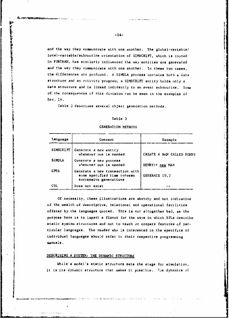
and the way they communicate with one another. The global-variable/

local-variable/subroutine orientation of SIMSCRIPT, which is rooted

in FORTRAN, has similarly influenced the way entities are generated

and the way they communicate with one another. In these two cases,

the differences are profound. A SIMULA process contains both a Cata

structure and an ectivity program; a SIMSCRIPT entity holds only a

data structure and is linked indirectly to an event subroutine. Some

of the consequences of this division cmn be seen in the examples of

Sec. IV.

'Table 3 deucrtues veveral object generation methods.

Table 3

GENERATION METHODS

Language Concent Example

SIMSCRIPT Generate a new entitywhenever 3ne is needed CREATE A MN CALLED HENRY

SLMILA Generate a new processwhenever one is needed HENRY:- new MAN

GPSS Generate a new transaction withsome specified time between GENERATE 10,3successive generations

CSL LDoes not exist

Of necessity, these illustrations are sketchy and not indicative

of the wealth of descriptive, relational and operational facilities

offered by the languages quoted. This is not altogether bad, as the

purpose here is to impart a flavor for the ways in which SPLs describe

static system structures and not to teach or compare features of par-

ticular languages. The redder who .s interested in the specifics of

4individual languages should refer to their respective programmingi manualIs.

DESCRIBING A SYSTEM: THE DYNAMIC STRUC'URE

While a model's static structure sets the stage for simulation,

it is its dynamic structure that makes it possibie. Thie dynamics of

I

-15- 14system behavior in all SPLs is r.:presented procedurally, that is, by

computer programs. While desirable, no nonprocedural SPLe have yet

been invented, although substantial success toward this end has been

achieved in limited areas [25].

At present, two SPLs have achieved widespread prominence and use

in the United States, and two others have achieved similar prominence

in Europe and Great Britain. These are GPSS, SIMSCRIPT, SIMJLA, and

CSL, respectively Interestingly enough, each presents a different

view of system dynamics. To understand why this is so, a historical

rathei than functional discussion seems appropriate.

The Concept of Simulated Time

Soon after academics and practitioneri recognized that simuiation&

of industrial and military processes could be conucted on digital com-

puters, they started to separate the simoilation-oriented portions of

computer programd from the parts describing the processes being siwu-

iated. A simulation vocabulary was developed; the first wotd in it

was probebly "clock." Program structurer began to reflect the concepts

embodied in the vocabulary.

Since time and its representation are the essence of simulation,

it was natural for it to be the first item of concern. If one could

represent th3 passage of time within a computer program and associate

Lhe execution of programs with specific points in this similated time,

one coud claim to have a time-dependent simulation prograo.

The first simulation clocks imitated the behavior of real one3.

They were counters that "ticked" in unit increments repreaenting

seconcin, minutes, hours, or days, provling a pulse for simulation

programs. Each time the clock ticked, a simulation coitrojlpro ram

looked around to see what could happen at that instant in simulated

time. ;het could happen could be determined in two ways: by pre-

dete truction or by search. Before going into theme two

techniques, me words are in order about simulation control programs.

-16-

Th.. Structure of Simulation Control ProIaMnC

The heart of every simulation program, and every SPL, is a tir

control program. Thia program is referred to in various publivatforis

as a clockworks, a simulation executive, a timing mechanism, a sequencing

set, and the llke . Its functLions are always the same: to advance

sitmulation timc and to select a subprogram for execution that performd

a spctfled simulation activity.

rThus, every simuletion program has a hierarchical structure. At

the top sits the time control program, at an intermediate level sitsimulation-oriented routines, at the bottom sit ioutinea that do basic

housekeeping functions such as input, output, and the computation of

mathematical functions. Every $PL provides a time control program;

when using an SPL, a simlation programmer does not have to write one

himoelf -- or even worse, invent onen

Depending on how the time control program works, a simulation

programmer miy or may not have to use special stateonts to interact

with the timing mechanism. Most simulation languages contain one or

msre Statements that permit a prograrsnr to organize system activities

in a time-dependent manner. Further on, thi4 3ection d* cczibes several

different simulation control program schemes and the ways in which a

programmer interacts with them.

First, it must be unde'stuod that every sriulation program is

compoyed of blocks of statements that deal with specific system activ-

ities. These blocks may be complete routines* or parts ot routines.

They have been calied events, activities, blocks, processes, and seg-

aentd. The distinctions between them will be clarified presently; at

the moment it is only necessary to understand that a simulation program

is composed ef identifiable modules that deal with different simulatijn

situations.

A simulation control progrcm can select a portton of code to

execute in either of t~p ways; by predetermined instraction or by

ihe words routine, subroutine, program, subprogram, and p:ocedure

are uted here irterchangeably.

-17-

search. Regardless of how the result is determined, the effect is the

same -- the execution of an appropriate block of code. Figure 2 blocks

out the basic structure of every simulation program.

Determination of

next executable

program segment

S

Fig. 2 -- Basic simulation structure

Simulation starts at I, where a model is initialized with sufficient

data to describe its initial system state and the processes that are

in Lotion within it. Based on information computed in the "next event"

block, S switches to the code block that corresponds to the proper

simulation activity.

The "search" method of next-event selection relies upon the fact

that when a system operates it moves from state to state in a pre-

determined manner. The times at which state changes occur tay be

random, and represent the effects of statistically varying situations,

but basic cause-and-effect relations still hold. Given that a system

is in state "A", it will always move into state "B" if certain condi-

tions hold; code block AB, say, must always be executed to effect the

change. A "search" method relies upon descriptions of activity-

producing system states and a scanner that examines system state data

to determine whether a state change can take place at any particular

clock pulse.

-18-

When a state change can be made, the code block representing it

alters data values to reflect the change. Since many system changes

take place over a period of time, some of the data changes are to

"entity clocks." These clocks are set to the simulated time at which

a state change is considered completed. *When the control program finds

that an "entity clock" has the same time as the master simulation clock,

it performs the activity associated with that clock, e.g., relegating

a working machine to idleness or causing an emptying tank to run dry.

State changes that happen instantaneously, either when a code block

is executed or as the result of some entity clocks equaling the sim-

ulation clock, cause new code blocks to be executed, new entity clocks

to be set, . . ., cause the system activities to be reexamined.

The efficiency of this rather basic scheme was first improved by

eliminating the uniform clock pulse. Since, in many simulations,

events do not occur on every clock pulse but randomly in time, a great

deal of computer time can be lost in scanning for things to do each

time the clock is advanced one increment. It is more efficient to

specify the time at which the next event is to occur and to advance

the clock to this time. As nothing can happen before this time, it

is unnecessary to search for altered system states. By definition of

the next event, no entity clock can have an earlier time. At best,

it can only be equal to the next event time.

The term "next-event simulation" was given to simulation programs

that stepped from event time to event time, passing over increments

of time in which no state changes occurred. All modern SPLg use the

next-event technique. The term critical event is often used in the

same spirit.

Two SPLs that do employ search are GSP [62] and CSL. In both, the

activity i the basic dynamic unit. An activity is a program composed

of a test section and an action section. Whenever simulation time is

advanced, all activity programs are scanned for possible performance.

If all test conditions in an activity are met, state-changing and time-

setting instructions in the action section are executed; if at least

one test condition is not mt, the action instructions are passed over.

-19-

A cyclic scanning of activity programs insures that all possibilitiesare examined and all interactions are accounted for.

In addition to the activities scan, GSP incorporates an event

scheduling mechanism that enables an activity to specify that some

system event is to take place at a determined time in the future.

Events that are not affected by other events, i.e., are not heavily

interactive, can be treated more efficier-ly this way, as repeated

scanning is not required to determine when they can be done.

When an activitv rcan is not employed, as is the case in GPSS,

SIMSCRIT, and SIMULA, all system events must be predetermined and

scheduled. The activity-scan and event-scheduling approaches are dif-

ferent solutions to the same problem; an activity scan is efficient

for highly interactive processes involving a fixed number of entities,

e.g., multiresource assignment problems in shops producing homogeneous

products; event scheduling is efficient for less interactive processes

involving large numbers o entities, e.g., simulations of job shops

producing special order products. Efficiency must be treated as a

multidimensional quality, of course. We must speak of -modeling effi-

ciency and programming efficiency, as well as computer running-time

efficiency.

The differences between activity scanning and event scheduling

orientations can be pointed out best by procedural desciiptions.

Event Selection Procedures

Take a simple shop situation in which a man and a machine must

work togethei to produce a part. Each has an independent behavior,

in that the man starts his day and ends it, takes coffee breaks, and

goes to lunch without regard for how the machine is performing, and

the machine suffers breakdow~as and power failures without regard for

what the man may be doing.

The Activity Scanning Approach. An activity approach to simulating

the processing of a part in this man-machine shop specifies the condi-

tiona for a job to start processing, and the actions that take place

when such conditions are met:

I!

-20-

Test section: if part is available AND

if machine is idle AND

if man is idle THEN do Action section

OTHERWISE return to timing mechanism

Action section: put man in committed state

put machine in committed state

!determine time man will be engageddetermine time machine will be engaged

set man-clock to time man will becomeavailable

set machine-clock to time machine willbecome available

return to timing mechanism

Emphasis is on the activity of producing the part, not on the

individual roles of the man and the machine. Periodic scanning of

the activity finds instances when all three conditions hold.

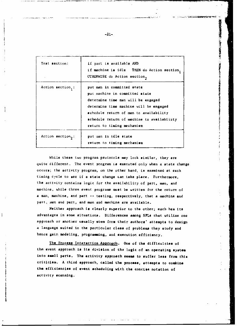
The Event Scheduling Approach. An event scheduling approach to

the same problem requires that three programe be written, one for the

man, one for the machine, and one for the part. The programs contain

both test and action statements, and are "menus" for situationa that

can take place whenever a state change event occurs. For example,

one event in the simulation of the above man-machine shop would be

the return of a man to the idle state from whatever activity he might

have been engaged in. The routine that represents the "man becomes

idle" event might look like;

-21-

tTest section: if part is available AND --

if machine is idle THEN do Action section1OTHERWISE do Action section2

2A

Action section I put man in committed state

put machine in committed state

determine time man will be engaged

determine time machine will be engaged

schedule return of man to availability

schedule return of machine to availabiiity

return to timing mechanism

Action section2 : put 4on in idle state

return to timing mechanism

While these two program protocol@ may look similar, they are

quite differpnt. The event program is executed only when a state change

occurs; the activity program, on the other hand, is examined at each

timing cycle to see if a state change can take place. Furthermore,

the activity contains logic for the availability of part, man, and

machine, while three event programs must be written for the return of

a man, machine, and part -- testing, respectively, that a machine and

part, Aan and part, and man and machine are available.

Neither approach is clearly superior to the other; each has its

advantages in some situations. Differences among SPLs that utilize one

approach or snotiier usually stem from their authors' attempts to design

a language suited to the particular class of problems they study and

hence gain modeling, programming, and execution efficiency.

The Frocess Interaction Approach. One of the difficulties of

the event approach is its division of thie logic of an operating system

into small parts. The activity approach seems to suffer less from this

criticism. A third approach, called the process, attempts to combine

the efficiencies of event scheduling with the concise notation of

activity scanning.

i

~-22-

A process can be defined as a set of events that are associated

with a system behavior description. The events are interrelated by

special scheduling statements, such as DELAY, WAIT, and WAIT UNTIL,

that interrupt the execution of a subprogram until a specified period

of time has passed or a stated set of conditions hold. DELAY and WAIT

are time-oriented and are effected through event scheduling techniques.

WAIT UNTIL, being condition-orlented, requires an activity-scan approach.

A process description thereby combines the run-time efficiency of event

scheduling with the modeling efficiency of activity scanning. SIMULAis a process-oriented language that has had several years of successful

experience and has undergone one revision [161. GPSS is a process-

oriented language with a longer history and even more widespread accep-

ftance. Although it is flow-chart-oriented rather than statement-oriented, the basic 1rocess concepts expressed here apply to it.

A key feature of process-orientation is that a single program is

made to act as though it is several programs, independently controlled

either by activity-type scans or event scheduling. Each process has

several points at which it interacts with other processes. Each process

can have several active phases; each active phase of a process is an

eveat. This is different from pure event or activity approaches that

allow an interaction only when all the actions associated with an event

or activity have been completed, e.g., when they return to the timing

uechanisp.

The programming feature that makes this scheme possible is the

reactivation point, which is essentially a pointer that tells a process

routine where to start execution after some time-delay conmand has been

executed. Figure 3 illustrates the concepts of interaction point and

reactivation point for prototype event, activity and process routines.

In Fig. 3a, there is one reactivation poirt and one interaction

point. An event routine always starts at the same executable statement,

and, while it may have several physical RETURN statements, only one can

be executed in any activation. When it is executed, it returns control

to the master control program, which selects the next event (previously

scheduled) to occur. All actions taken within the event routine take

I

[ ".

! _ _ _ _ _ _ _ _ _ _ _ _ _ _ _ _ _

___-___ __,.__ __ _ ___ - . . .. " - . _ . . . _ _ _ L

-23-

reactivation EVENT ARRIVAL routine declaration

point - -

SCHEDULE AN ARRIVAL AT 100.0 creation of a futureinteraction point

actions to change system state

RETURN interaction with otherevents takes place

END when routine returns

to control program

(a) Prototype event routine

reactivation ACTIVITY BERTHING routine declaration

point - jtests to determine if act activity tests

can occur

actions taken during berthing executed if testsindicate activitycan occur

RETURN interaction with otheractivities when j

END routine returns tocontrol program

(b) Prototype activity routine

reactivation PROCESS SHOPPING routine declarationpoint - soctions to start shopping

reactivation WAIT 15 MINM'ES interaction pointpoint actions to shop

reactivation WAIT UNTIL SERVER IS FREE interaction pointpoint -

actions to check out

reactivation DELAY 10 MINUTES interaction point

polnt -actions to return home

SCHEDULE SHOPPING IN 15 KINUTES creation of futureinteraction point

actions to renew shopping process

END interaction point

(c) Prototype process routine

Fig. 3 -- Concepts of interaction point and reactivation point

-24-

place at the same simulated time, independently of other events. Theevent is not totally divorced from other events, as all events share

the same system data.

In Fig. 3b, there is again only one reactivation point and one

logical interaction point. If an activities test section permits them

to take place, all actions occur at the same simulated time.

Figure 3c presents a sharply different picture, with many reacti-

vation and interaction points.

Figures 3a, b, and c show that reactivation and interaction points

always come in pairs. A minute's reflection will show that this has

to be so. At each interaction point a reactivation point is defined,

which is the place execution will start when the indicated time delay

elapses or the condition being sought occurs. Within a process routine,

all actions do not necessarily take place at the same simulated time,

but through a series of active and passive phases.

The reader should be able to see the differences among the event,

activity, and process prototypes and get a qualitative feel for how

the three differ.

Each modeling scheme has distinct virtues. Each can be shown

to be advantageous in some situations and disadvantageous in others.

There are no rules for selecting one scheme over another in given

situations, nor is it likely that any such rules will ever be stated.

The universe of possible simulation models is so large and so diverse

that there would undoubtedly have to be more exceptions than firm rules.

Several points, however, are clear:

A language employing event scheduling gives a modeler precise

control over the execution of programs.

A language employing activity scanning simplifies modeling multi-

resource systems by allowing conditional statements of resource avail-

ability to be specified in one place.

A procest-oriented language reduces the number of "overhead"

statements a programer has to write, since he can combine many event

subprograms in one process routine. In addition, the overall flow of

a system is clear, as all logic is contained in one routine rather

than several.

-25-

On the other hand, there is nothing one scheme can do that another

cannot. Questions of feasibility must be separated from questions of

efficiency. Also, as more experience is gained with languages employing

these schemes, more efficient algorithms will be developed and efficiency,

per se, will become less of a problem. Eventually, modeling esthetics

will become an overriding consideration.

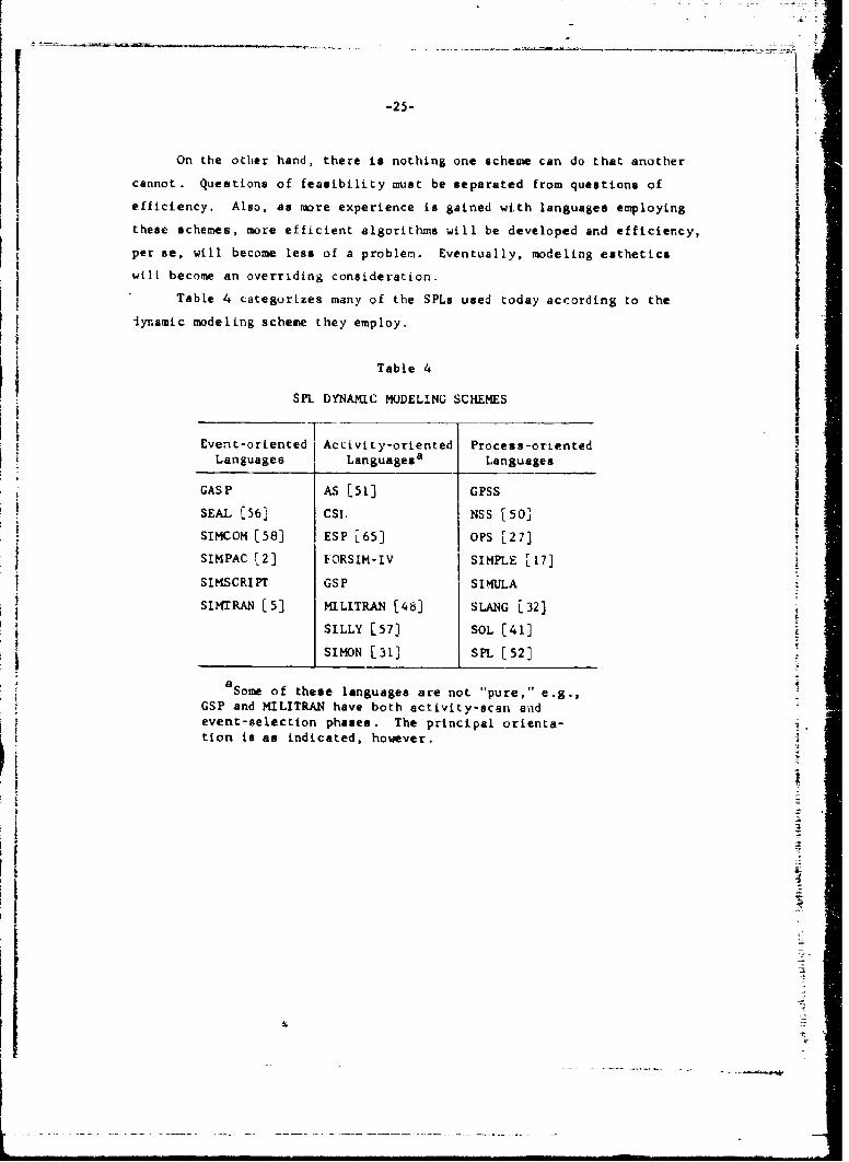
Table 4 categorizes many of the SPLs used today according to the

lynamic modeling scheme they employ.

Table 4

SPL DYNAMC MODELING SCHEMES

Event-oriented Activity-oriented Process-orientedLanguage Languagesa Languages

GASP AS [51] GPSS

SEAL C56] CSL NSS [50]SIMCOM [58] ESP [65] OPS [27]SIMPAC [2] FORSIM-IV SIMPLE [17]

SIMSCRIPT GSP SIMULA

SIMTRAN [5] MILITRAN [48] SLANG [32]

SILLY [57] SOL [41]

SIMON [31] SPL [52]

aSome of these languages are not "pure," e.g.,GSP and MILITRAN have both activity-scai andevent-selection phases. The principal orienta-tion is as indicated, however.

Ii.

p

-26-

I1. SI{UILATION PROGRAMMING LANGUAGE FEATURES

SPECIFYING SYSTEM STRUCTURE

Every SPL must have some way of describing system structure in

both its static and dynamic aspects. Section Ii discussed the principal

features needed for this; Table 5 summarizes them.gLi

Table 5

SYSTEM MODELING FEATURES

~Ststeamint s to.Deline classes of objects within a system

Adjust the number of objects within a class

as system conditions changeDefine properties of system objectsDescribe relationships among system objectsDefine activities, events, or processesOrganize events or processes

Programs to:Select activity, event, or process subprograms

for execution

F Advance simulation time

REPRESENTING STATISTICAL PHENOMENA

To model the real world, one must have a way of modeling random

factors and effects. It i necessary to model undertainty and vari-

ability with equal ease.

Uncertainty enters into models in statemenL such as;

In situation X, 15 percent of the time Y will occurand 85 percent of the time Z will occur. Given thata system is in state X, some probabilistic mechanism

is required to select either state Y or state Z as thenext state.

Variability enters into models in statements such as,

The time to travel from A to B ha s &n exponentia!distribution with a mean of 3 hours, or the numberof customers expected to arrive per hour has a

Poisson distribution with a mean of 6. A proba-bilistic mechanism must be available for generatingsamples from statistical distributions.

IIJ.

!

I r

-27-

In reproducing variability or uncertainty, a simulation model

must have a way of generatinK random variables. A basic feature of

tvery SPL is a random-number generator. Additional feaLures are pro-

! grams that transform random numbers !nto variates from various statis-

tical distributions and perform related sampling tasks.

A process is random if predictions about its fuure behaviorcannot be improved from a knowledge of its past behavior. A sequence

of numbers is a random sequence if there is no correlation between

the numbers, i.e., if there is no way to predict one number from another.

Random numbers are needed to introduce uncertainty and variability into

models, but because of the kinds of experiments that are performed with

simulation models, truly random sequences of numbers are not adequate.

One must have reproducible sequences of numbers that are, for all

intents and purposes, random so far as their statistical properties

are concerned.

Pseudorandom numbers, aq reproducible streams of randomlike

numbers are called, arf generated by mathematical formulae in such a

way that they appear to be random. Since they are not random, but

come from deterministic series, they can only approximate the indepen-

dence of truly random number sequences. Every simulation study calls

for verification of random-number generators to insure that the sta-

tiatical properties are adequate for the experiment being performed

[20]. Every SFL must have a procedure for generating statistically

acceptable sequences of pseudorandom numbers.

Pseudorandom number sequences always consist of numbers that are

statistically independent and uniform' istributed between 0 and 1.

Generation of a pseudorandom number ra a real number somewhere

in this range.

Pseudorandom numbers can be used directly for statistical sampling

tasks. They can represent probabilities in a decision sense or in a

sampling sense. The model statement:

Make decision D 60 percent of the time,

Make decision D 40 percent of the time,

-28-

can be implemented in an SPL by generating a pseudorandom number and

testing whether it lies between 0.0 and 0.60. If it is, declstor D

is taken; if it is not, decision D2 is taksi. For a sufficlenrly large

number of samples, D1 will be selected 60 percent of the time, but the

individual selections of D or L will be independent of previous1 2

selections.

The model statement:

Produce product P 20 percent of the time,t

Produce product P2 10 percent of the time,Produce product P3 15 percent q the time,

3Produce product P 20 percent of the time,

4Produce product P 35 percent of the time,

5

can be implemented in a similar way by sampling from a cumulative

probability distribution. A random product code can be drawn from

the above product mix by putting the product frequency data into a

table surn as

Product type Cumulative probability

1 0.20

2 0.303 0.454 0.655 1.00

In this table, the oifference between the successive cumulative prob-

ability values is the probability of producing a particular product;

e.g., product 3 is produced 0.45 - 0.30 - 0.l. or 15 percent of the

time. When a pseudorandom number is generated and matched against the

table, a random product selection is made. Fcr example, generating

the number 0.42 selects product 3. Since numbers between 0.30 and

0.45 will be generated 15 percent of the time, 15 percent of the product

numbers generated will he Lype 3.

While this type of sampling is useful for empirica, frequency

distributions, it is lesA useful for sampling from gettistical

: ii

-29-

distributions such as the exponential and normal. lo use a cable look-

up procedure suc. as the one describec. above, and sarple accuratcely

in the tails of a statistical distributioa, large tables must be stored.

Generally, a simuiation cannoc afford the tables, needing the storage

for model data and program. ALgorithms rather than table look-up IA

procedures are used.

Sampling algorithms are of many ki.nds. Some distributi-ons are

easily represented Ly exact mathematical formulae, acme muat be approx-

imated. All sampling methods operate in the same way insofar as they

transform a pseudorandom number to a number from a particular statistical

distribution. References 10, 49, and 63 discusb such procedtures in

detail. As simulation is almost always performed using sampling. pro-

cedures that can generate samples from standard statistical distribu-

tions are mandatory in an SPL.

In conducting sampling experiments, which is what simulations

really are, one is interested In control and precision as well as

accura.y of representation. The topics dealt with so far have all b en

concerned with representation.

Control is necessary when one is using simulation to test and

compare alternative iules, procedures, or qualities of equipment. When

several simulation runs are made that differ only in one carefullyialtered aspect, it is important that all other aspects re.ain constant.

One must be able to introduce changes only where they are desired.

This is one of the reasons for requiring reproducible random-number

streams. A fCature that aids in this is the provision of multiple

streams of pseudorandom numbers. Having more than one stream enables

parts of a model to operate independently, as far as data generation

is concerned, and not influence other parts. For example, when studying

decision rules for assigning men to lobs, one does not want to influence

the goneration of Jobs inadvertently. Multiple pseudorendom number

stream increase a programmer's control over a model.

One also wants to be able to control the generation of random

numbers if doing so can reduce the variability of simulation generated

performanca figur,.s. For example, it is always eesirable to make the

variance of the estimate of tne aierage length of a waiting line within

U=

-30-L

La aimu h ton model as small as possible. The reduction of sample

varianc-e is a statistical rother than a programing problem in all but

one reapect; a progre.,mer should be able to control the generation of

pseudorandom numbers if this is required. One known way to reduce

variance is to use antithetic variates in separate simulation runs;

this .s discussed in [20]. As the generation of a stream of ariatesr

4 that .-%re antithetic to a given stream involves no more tian a simple

subt crion,* this feature should be present in an SPL.

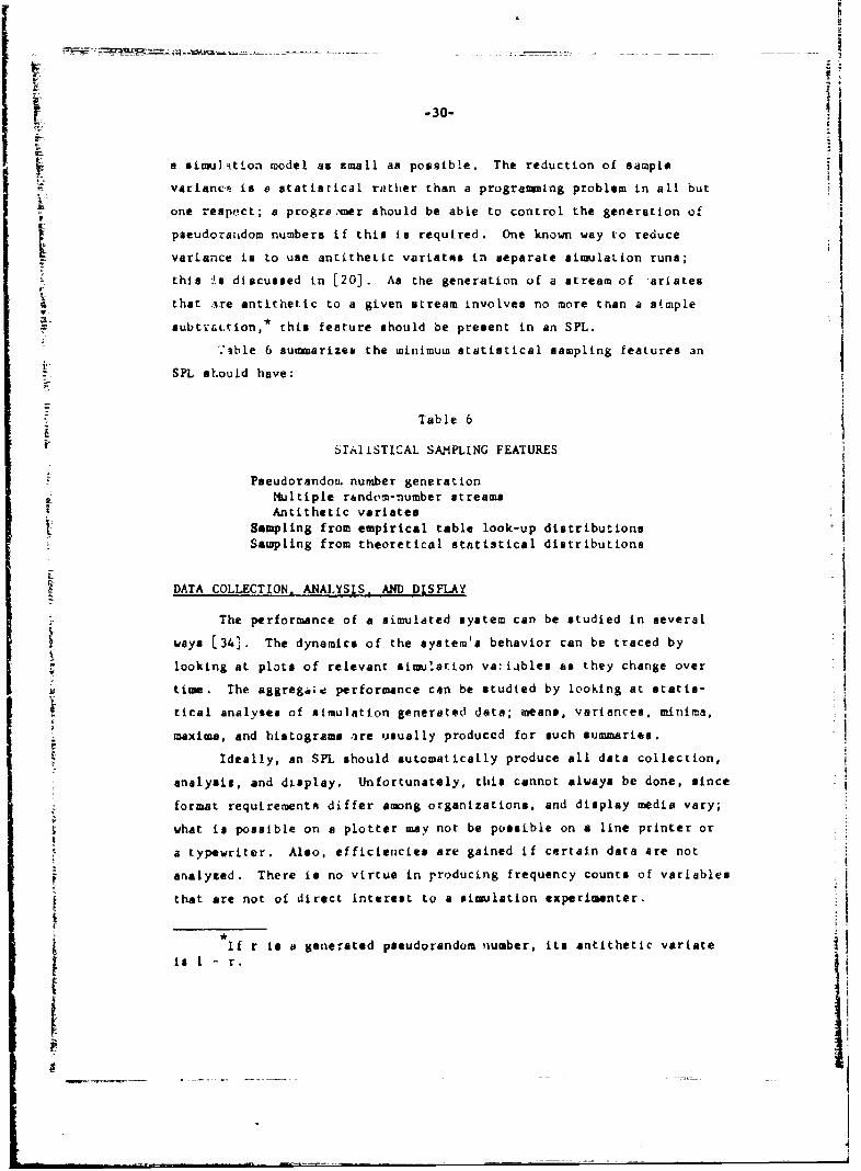
.able 6 summarizes the minimuw statistical sampling features an

SPL sh.ould have:

Table 6

r STAlISTICAL SAMPLING FEATURES

Pseudorando. number generationMultiple rindom-number streams

Antithetic variatesSampling from empirical table look-up distributionsSampling from theoretical statistical distributions

DATA COLLECTION, ANALYSIS, AND DISFLAY

The performance of a simulated system can be studied in several

ways [34]. The dynamics of the system's behavior can be traced by

looking at plots of relevant simulation va:ijblea as they change over

time. The aggreg4 ,e performance can be studied by looking at statis-

ftical analyses of simulation generated data; means, variances. minime,

maxima, and histograms are usually produced for such summaries.

Ideally, an SPL should automatically produce all data collection,

analysis, and display. Unfortunately, this cannot always be done, since

format requirementn differ among organizations, and display media vary;

what is possible on a plotter may not be possible on a line printer or

a typewriter. Also, efficiencies are gained if certain data are not

analyzed. There is no virtue in rroducing frequency counts of variables

that are not of direct interest to a simulation experimenter.

i If r is a generated pseudorandom number, its antithetic variate

I I - r

-31-

There are several topics to discuss in this general area: how

data collection is specified, what data collection facilities should

be provided, how display media can be used, how display fo. -a are

specified, and what data analyses should be performed.

Data Collection Specification

The best one can say of a data collection specification is that

it is unobtrusive. While data collection is necessary, statements that

collect data are not per se part of a simulation model's logic and

should not obscure the operations of a model in any way. People find

that debugging is difficult enough without having to deal with errors

caused by statements intended only to observe the behavior of a model.

The ultimate in unobtrusiveness ia to have no specification

statements at all. Being free from them clearly eliminates any diffi-

culties they may cause when reading or debugging a simulation program

code. Unfortunately, having no specification at all means that every

possible piece of data Must be collec.ed ir every possible way, at the

risk of neglecting to collect something an analyst may want. In small

models this is probably worthwhile. In large models it can !ead to

,nacceptable increases in core storage requirements and program running

times. GPSS collects certain data automatically and allows a programmer

to collect other data himself; GASP does something similar.

A reasonable alternative is a linguistically natural set of data

c !lect.on statements that can be applied globally Lu a model. Being

linguistically natural, they will be easy to use and clearly differ-

entiable from other types of programning statements. Being globally

applicable, -hey need be written only once, rather than at each place

a particulat item of data to be collected appears.

Barring this, data can be collected through explicit procedural

piogram statements. Data-collection specification statements of this

sort are no different from normal variable assignment statements or

subroutine calls. They are the easiest to implement in an SPL, but

the most obtrusive and difficult to deal with. Most SPLs provide

facilities of this kind. SIMSCRIPT II [39] has a capability for global

data-collection specification.

l*

-32-

Data Collection Facilities

One must be able to collect a variety of data, since one should

be .'le to compute all the statistics an analyst might want about a

simulation variable. This includes counts of the number of times a

variable changes value, sums, sums of squares, maxima and minima of

these values, histograms over specified intervals, cross-products of

specified variables, time-integrated sums and sums of squares for time-

dependent data, and time series displays. Simulation is a statistical

tool, and statistically useful data are required to use it.

Naturally, some data are easier to collect than others. Table

7 lists the minimum data one should be able to collect.

Table 7

DATA COLLECTION FEATURES

Number of observations, maxima, and minima for all variablesSums and sums of squares for tirme-independert variablesTime-weighted sums and sums of squres for time-dependent variablesVariable valu-± histograms for time-independent variablesTime-in-stdae histograms for time-dependent variablesTime series plots over specified time intervals

These data should be easily collectable with specialized ctatements.

One should be able to collect any other data without extreme difficulty.

An important feature of an SF!L is that it allow reasonably free access

to all model data.

Data Analysts

One should not have to program the analysis of data for standard

statistical calculations, such as the computations of means and variances.

If global specifications are employed, names attached to statistical

quantities should invoke calculations when the names are mentioned. If

data collection statements are used, standard functions should operate

on named data to compute the necessary quantities.

Table 6 shows the minimum analysis one should be able to perform

from collected data. If the data are present, one would also like to

have functions that compute correlation coefficients and spectra [2i].

K .._ ...

-33-

Table 8

DATA ANALYSIS FEATURES

MeansVariances and standard deviationsFrequency distributions

Display Media

Standard statistical information is easily printed on typewriters

and line printers. Time series plots and histograms are enhanced by

graphic display. As this type of information derives most of its impact

from visual observation, there is little reason it should not be pre-

sented this way. Advanced SPLs should have routines for charting

results, either by simulating a plotter on a line printer or by dis-

playing results directly on a plotter [13], [23], [62].

Today, with a growing number of large-scale computing systems

making use of cathode ray tube displays (CRTs), these devices are being

used more and more for displaying simulation output [54]. Two situa-

tions lend themselves to CRT application.

In the first situation, the CRT is used only to produce attrac-

tively formatted graphs and reports. The dp,,ice is not viewed on-line;

pictures are made and used in lieu of printed reports. There is no

doubt that programmers can use enhanced graphical capabilities if given

the opportunity. Generally, no changes need be made to a SPL to let

them do so, other than providing access to general system software

routines. To be specific, a programmer should be able to call upon

library plotting routines from a SINSCRIPT or GPSS program.

The second situation is the more glamorous, with output produced

on-line as a program is executed. Given a language and an operating

system that lets a programmer interrupt a running program, alter system

parameters and variables, and then continue simulating where he left

off, an entirely new type of simulation debigging and experimentation

is possible. This type of interactive, adaptive dialogue between model

and programmer makes on-line, evolutionary model design possible, changes

the economics of sequential, optimum-seeking experimentation, and adds

_34-

a valuable dimenion to program debugging. Several researchers, at

The RAND Corporation and elsewhere, are currently working in this area

C17], [30].

Specification of Dialy Formats

There are probably as many types of output statements as there

are people who write programming languages. Each type, being a little

different, emphanizes one or more aspects of output control at the

it- expense of others. Styles range from no specification at all (GPSS),

Ithrough format-free statements (SIMSCRIPr II) and formatted statements

(CSL), to special report forms (SIMSCRIPT). There are times when each

style has its merits, and a fully equipped SPL will have a variety of

output display statements.

Four types of display statements that exist in present-day SPLs

are:

(1) Automatic output in a standard format (GPSS, GASP):

Is a time-saver for the programrner and P boon in reasonably@mail models where all data can be displayed at a reasonablecost.

Does not force a beginning simulation programmer to dealexplicitly with output.

Is only as good as the exhaustivenesa of its contents.

Is often unsatisfactory for formai reports, forcing subse-_ quent typing and graph prepdration.

(2) Format-free output (SIMSCRIPT II):Enables a programmer to control the display of informationwithout regard for formats.

Is adequate only if it covers all the data structures in alanguage.

Is most useful for debugging, error message reporting, andprinting during program checkout.

(3) Formatted output (CSL):

Requires the most programmr knowledge, but provides themaximum control of information display.

Is traditionally the most difficult part of many programminglanguages, insofar as the greatest number of errors are made

by novice program rs in format statemnts.

II - - ---- =-..-......- ---- ~-~-- ----- ~ '.-~. . .

.35-

(4' R~eport Generator!! (SIMSCRLFE, (,sr>

Are the easiest way of producing specially designed reports.

Must have a complete complement of control facilities tocover all reporc situstiona.

Can be a nuitance to use in very simple situations.

Usually gemarate an extremely large amount of object code.Are efficien- from a programming standpoint, but not from

a core-consumption poitt of view.

Since the production of reprts im the primary task of all pro-

grams, whether they are run for checkout, for display of computed

results, or for preparation of elaborate management reports and charts,

a good SPL should contain statementh adapted to all display situations.

Going back to the discussion of data collection, a programer should

not have to spend a great deal of his time writing output statements.

He should be able to concentrate on model construction and programming

and not have to dwell at length on conventional output tasks. He

should be able to spend time on sophisticated output statements, how-

ever, to produce displays that are unusual or that deal with exotic

display devices.

ION!TORING AND DEBUGGING

Two essential requirements of all SFLs can be served by the same

set of programming facilities. SPLz should be able to assist in:

(1) Program debugging; and in i(2) Monitoring system dynamics.

Debugging can be difficult in high-level programming languages,

L as there is generally a great deal of difference between source and

object codes. Errors can be detected during compilation and execution

Lhat are only distantly related to source-language commiands, Moreover,

when an SPL is translared into an intermediate POL, as was originally

done in SIMSCRIFr and CSL, execution error messages are often related

to the intermediate language and not the programmer's source statements.

These messages, while meaningful to an expert, can mislead a noviceSPL programmer.

Debugging is also difficult because the flow of control in a

simulation ii stocha!tically determined. Moreover, it can be difficult

-36-

to obtain a record of the flow of control, since an SPL-designed

"timing routine" or other form of control program is the originating

point for all event cella. In some languages, it is impossible to do

so. Without program flow information, and information about the system

state at various times, some simulation program errors can be found

only by luck.

The debugging features an SPL should provide are listed in Table 9.

Table 9

VEBUGGING FEATURES

Report compile and execute-time errors by sourcestatement related messages;

Display complete program flow status when an execute-time error occurs. This means displaying the entrypoints and relevant parameters for all function andsubroutine calls in effect at the time of the error;

Provide access to control information between eventexecutions. This allows event-tracing during all orselected parts of a program, and use of controlinformation in program diagnostic routines.

These same facilities are needed for monitoring system dynamics.

As one use of simulation is the study of system behavior, one must be

able to view sequences of events and their relevant data to observe

system reactions to different inputs and different system states.

Event-tracing is an important tool for this kind of study.

In an event-oriented SPL, debugging and monitoring features will

undoubtedly be implemented differently from the same or similar fea-

tures in activity- or process-oriented SPLs. This is not important.

The basic issue is whether some basic facility exists for assisting

in program debugging and for doing program monitoring.

INITIALIZATION

Because simulation is the movement of a system model through

simulated time by changing its state description, it is important

that an SPL provide a convenient mechanism for specifying initial

1I -.37-

system states. In simulations dedicated to studying start-up or

transient conditions, a convenient mechanism for doing this is manda-

tory; in simulations that only analyze steady-state system performance,

it is still necessary to start off at some feasible system configuration.

Some Sas start simulation in an "empty and idle state" as their

normal condition and require special efforts to establish other con-

ditions. They rely either on standard input statements, formatted or

unformatted, to read in data under program control or on preliminary

programs that set the system in a predetermined state.

An alternative to these procedures is a special form that reduces

the initialization task to filling out a form rather than writing a

program. While adequate in a laL~e number of situations, this alter-

native suffers from being inflexible. As with the preparation of

simulation reports, the correct anewer lies in a mixture of initial-

ization alternatives.

Another aspect of initialization is the ability to save the state

of a system during a simulation run and reinitialize the system to

this state at a later time. This facility is crucial in the simula-

tion of extremely large systems, and in coniducting sequential exper-

iments. One should be able to save all the information about a program,

including relevant data on the status of external storage devices and

peripheral equipment, and restore it on command at a later date.

OTHER FEATURES

There are a number of non-operatioal features that must be taken

into con.ideration when designing or selecting an SPT. A manager or

analyst is interested in program readabllity; coimunication of the

structure, assumptions and operatlone of t model i2 fi.poxtant if the

model is to be used correctly. A waniger i~s also, interested in execu-

tion efficiency; simulations cen rp.:ui.r2 large numbers ct txperiment.9

runs, and the cost par run =it be low enough to make n ptoject eco-

nomical. On the other ha.ad, a manager must baloa.e the costs of pro-

ducing a prog sam against prograL exeutiL c.sNC. (Wple mode"irlg

languager may compile and aexcute .oa efficiently than impler

languages, but the:' make probleas solvable in a shorter period of-

-38-

time. If total problem sulving tim is important rather than computer

time costs, the evaluation criteria change.

SPL documentation is important to applications and system pro-

gramaeru. An applications programmer needs a good instruction manual

to learn a language and to use as a reference guide. As an SF1L becomes

more complex the need for good documentation increases. Syetems pro-

grawmrs need documentation to be able to maintain an SPL. This

documentation must allow them to install the language in the computing

system; with today's complex, hand-tailored systema this is becoming

more difficult. It must also provide enough infox.mation for them to

make modifications in the SPL itself as translator errors are dis-

covered. It is less important that users be able to modify an SPL,

either to change the form of statements or to add new ones, but this

can be an important consideration in certain instances. Some languages

in fact are designed to do this easily [16], [38., [50].

i i

_ _a

.-- -~ -___________- - - - ~.-- - - - -- ---

-39-

IV. SOME EXAMPLES OF SPLS

This section illustrates four SPLa: SIMSCRIPT II, an event-

oriented language; SIMULA, a process-oriented language; CSL, an

activity-oriented language; and GPSS, a transaction-oriented language.

With the exception of the SIMSCRIPT II example, which appear# for the

first time in this Memorandum, the illustrations are taken from pub-

lished descriptions of the respective languages. The examples differ

in detail and specificity, but are nevertheless representative of the

concepts the languages employ. As they have been taken from other

sources with only a surface editing, they also differ greatly in style

and format.

Because the SIMSCRIFT II example was written especially for this

Memorandum, it is the most detailed and illustrates the greatest number

of features. Consequently, the reader may tend to judge SIMSCRIPT

II a superior language. He should not make such a judgment solely on

the basis of these examples. Ideally, they should all be comparable

and not bias the sought-after end, which is the explication of their

different approaches to providing the SPL features discussed in Sec.

III. We can only hope that our inability to procure "equally repre-

sentative" examples will not detract from our purpose.

The concepts the languages employ have all been described in

previous sections and readers should be able to follow the examples

without a thorough understanding of each. The format of the following

subsections is: description of a model, simulation program for the

model, discussion of the program.

SIMSCRIPT I: AN EVENT-ORIENTED LANGUAGE

The model used in this example is the "executive-secretary system"

described in [34). The program conforms as closely as possible to

the description given in [34) and the flowcharts of its events.

Although GPSS is process-oriented, in the sense that its modelstake a synoptic view of systems, its basic orientation is with theflow of transactions rather than the occurrence of processes.

-40-

The Modul

We assume that executives In an office system have two types oi

tasks: they procesa incoming communications (invoices, requests for

bids, price queries) and handle interoffice correspondence. The tasks

are not independent of one anotler; the former are produced by mecha-

nisms external to the office system, the latter arise during daily

operations. As they result in similar actions we can treat both the

same way, through an event that "discovers" a task. Other events

assign tasks to secretaries, schedule coffee breaks and departures

for lunch, and handle the review of completed secretarial task6.

Table 10 lists the objects that "live" in the office system -- which

we shall call entities from here on -- and their attributes.

Table 10

SYSTEM ENTITIES AND THEIR ATTRIBUTES

;Execu tive Secretary Tas k

Position: Skill in typing: Type:hanager words/minute InvoiceSenior errors/l00 words Price qaotationJunior Bid

Skill in dictation: TelephoneState: words/minute T tionDictation

Busy errors/100 words TypingAvaiableSkill in office work-

On break S Characteristics:general rating 1-100

State: Secretarial requirementsBusy Probability of requiringAvailable a follow-up taskOn brak

Given the esetic structure defined in Table 10, the nature of

the task-discovery event, and sou* logic not yet described, we can

construct a flowchart model of the actions that take place when a

request enters the system. This model is illustrated in Fig. 4.

Numbers to the left oi each flowchart block refer to comments in the

body of the text that iescrib. the operations that take place within

the block. The SISCRIPT II program for the model follows the

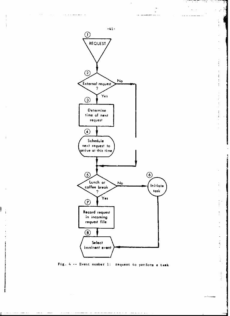
-41-

10

RE QUEYST

4

REQUESTExternal request No

Yt. S

0

Determine

time of nextrequest

(4)

Schedulenext request to

arrive at this time

5

Lunch or Nocoffee break Initiate

? task

Yes

Record requestin incomingrequest file

Select

imminent event

Fig. 4 Event number 1: request to perform a task

-42-

flowcharts and their description. The flowcharts and their respective

programs differ somewhat as the flowcharts are simplified for the sake

I: of clarity.

Block I is the entry point to the flowchart. It contains a name

that will be used in subsequent flowcharts to refer to the "task

request" event. The directed arrow leading from it is a symbol com-

monly used to indicate a path and direction of flow.

Block 2 is a decision block that splits the logical flow, depending

on the kind of request that has just occurred. To understand how this

block operates we must understand the concept of an event occurrence.

An event occurs when its "time arrives," the time having been

previously recorded by an internal scheduling block or observed on an

input data card. The precire iechanism that cccomplishes these tasks

need not be stated here. It suffices If the reader understands that

there i- some mechanism operating in the background of the simulation

program, obsf. L.g data cards and previously scheduled events, ordering

them by their event times, end "popping thea' up" when their time

arrives. This in fact ts the function of the event selection block

(Block 8). The reader will notice that every event terminates with

an event selection block. It ii in event sclection blocks that time

diocrim'.natione are made. events selected, and the si= lation clock

advarced.

Wheu a request event is poppeJ up, the siulation prog,'am hls

access to information associated with it, e.g., how it wae caused.

The model is .ble to look at this ifoLmatLion and take actLon on it.

If the request is for an inttrnally generated task, the flowchart

lead4 d'-ectly to Block 5, where a question is aekal to see 'i office

workers are available to process the request. If the request is for

mn externslly generated task, the program pauses in Blocks 3 and 4 to

read inforuatLon about the ntxt arrival from en external deta source,

and schd|le its arriv'l at sciae future time. 'ilien it does so it

records a mem of a request ariival and its time on a calend"r of

events scheduled to occur. This calendar is part of the selection

1re¢o|riom eaployel in sequencing events and adUancing simularinn time.

Theas operations are performed by the SIW RIFr II system atet do uot

have to be prograwmd explicitly.

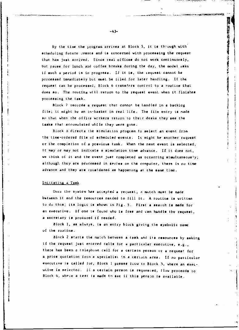
.-43-

By the time the program arrives at Block 5, it is th-ough with

scheduling future -.vents and Ls concerned with processing the request

that has just arrived. Since real offices do not work continuously,

but pause for lunch and coffee breaks during the day, the model jskr,

if such a period is in progress. If it is, the iequest cannot be

processed immediately but must be tiled for later handling. If the

request can be processed, Block 6 transfers control to a routine that

does so. The routire will return to the request event when it finishes

processing the task.

Block 7 records a request that cannot be Landled in a backlog

file; it might be an in-basket in real life. The file entry is made

so thdt when the office wcrkers return to their desks they see the

tasks that accumulated while they were gone.

Block 6 directs the simulation program to select an event from

the time-ordered file of scheduled events, it might be another rquest

or the completion of a previous task. When the next event is selected,

it may or may not indicate a simulation time advance. If it does not,

we think of it and the event just completed as occurring simultaneously;

although they are processed in setres on the computer, there is no time

advance and they are considered as happening at the same t;me.

IniLiatinR & Task

Once the system has accepted a request, a awtch inust be made

butween it and the resouxces ne.ded to fill it. A routine is written

to do this; its logic is shown in Fig. 5. First a search is made for

an executive. If one is fovnd who is free and can h&ndle the request,

a secretary is procured if needed.

Block 1, as always, is an entry block giving the symbolic name

of the routine.

Block 2 starts the ma:h between a task and its resources by asking

if the request just entered calls for a particular executive, e.g.,

there has been a tnlephone call for a certain person or a request for

a price quotation from a specialist 4n a certain area. If no particular

executive is called for, Block I passes ticiw to Block 3. where an exec-

utive is selected. l a certain person is requesLed, flow proceeds to

Block 4, whe1 e a test is made to see it this person is available.

I

-44-

NI AT

TASK

Is44 L heIYe

Yes No ri *.*C ,ia il

yety~sac

aig 5 W nr .*onolatOkwtYi

161

-45-

Block 3 is typical of a functional block whose description is

short but whose programming content might be large. A procedure to

select an executive can be brief, e.g., managers can do everything,

senior executives can do everything except give price quotation@,

junior executives can only answer tfe telephone; or it can be long

and elaborate, e.g., an executive is selected whose personal qualLfi-

cations as listed in his personnel file match the requirements of thetask according to a complex and computationally intricare formula.

Many of a simulation model's key assumptions are built into blocks

such as this.

When an executive is selected, Block 3 transfers to Block 4, the

block to which control is passed if a particular execu:.ive is called

for.

Block 4 asks if the executive requested in Block 2 or selected

in Block 3 is available. It does so by examining the executive's state

(status code); if the code is "available," the executive is free to

handle the request, if it is "bury" or "on break," he is not. Once

again, as in. Block ', the flow logic i split depending on the answer

to this question.

If the selected executive is available, flow passes to Block 8,

where proccssing of the task continmes. Before vs consider these

actions we should discuss what happens if the executive is not available.

Block 5 asks if a subttitute is availabie for a busy executive,

implying that a substitution can be made and that a procedure exists

for finding one. This *ituation is a littiv like that of Block 3,

where ,in executive to, selecti.d for a particular type of task.- Block

5 could be expanded Co a series of blocks describtng a procedure for

aclectl.rig a subatitute, tcbting for his availabi'ty, selecting another

substitute i. necessary, and so on until all possible candidates are

tred ard accepted or rtjected. In our simplified model we do not do

this. We only indicate that if a substitute cannot be found, control

2aases to Block 6, which files the unprocessed task.

Block 6 of this event is identical to Block 7 of the request event;

it 0i,4s information about the request for later p'.ocesaing. !.is block

apnea s in the simulation model whenever a request cannot be processed

and A,,%t be "remembered."

-46-I

In Bloc.:" 7 control is pasoad via an event selection block backto the "Liffekeepln&," me,&harism of the sisi-ation program. Since the

c rrent request cannot be processed, tht model must look at its calen-

dar of scheduled eventa to determine what to do next.

Returning to the case where an executive is available to process

a request, we ask next in Mock 8 if d vecretary )s alac needed. She

will be if the rzquest is for dictation or for some task where instruc-

tions must be given; ahe w.1_ not be if the task is simply answering

a telephone call. This question can be answerftd in a number of ways

in an operating computer program; am with most questions of this type,

we leave the description of decision-making at the macro level, namely,

that a decision has to be made.

Block 9 starts the flow path for the case where a request can be

honcred by an executive alone; it determines the amount of time he

will spend on the task.

Block 10 puts the executive in a "busy" state so that he cannot

be called on tr do another task while he is working on this one. He

will remain in this stdte until the "executive available" event occurs;

this is scheduled in Block i1 to happen after the lapse of the pre-

viously determined amount of time.

Before proceeding with the aimlation, the mode] must ask if pro-

ceasing this task, e.g., answering a phone call, induces another task,

e.g-, writing a memo. This is done in Block 12. If e task is not

induced, flow passes to Block 7, where the model is instructed to

selEct another event and proceed with the simulation. If a task is

induced, Block 13 determines its characteristics and passes them on

to Block 14, where the induced task is scheduled to be requested.

Flow then proceeds to Block 7.

If, back in Block 8, we foune that a secretary was needed to work

along with the executive, control would have passed to Block 15, where

a secretary must be selected before a task starts. This logic can

pair a particular secietary with an executive, pool all secretaries

so that they are available to all executives, or employ tome imediate

3cheme. As was done in selecting an executive, when a secretary is

chosen, her status code mui t be tested to see if she is available.

r

_°-i-- - - --- _ _ _ _ _

-47-

Block 16 performs this test. Like Block 5, it can be considered

a macro block in which alternaLives and availabilities are tested

until a decinion is reached. If a secretary is not available, a

request cannot be processed and must be filed along with other unpro-

ceased requests.

Once a secretary is found, Blocks 17, 18, and 19 determine the

time the executive and secretary will spend on the job, put the secre-

tary in the "busy" state, and schedule the time when her work will be

reviewed. It is not necessary that the executive and the secretary

work together on the task for the same period of ttwe; separate events

are provided to schedule cheir release from the task at different times.

The release times can be the same, however, if the task it a cooper-

ative effort.

Block 19 transfers control to Block 10 after completing its func-

tion, picking up at a part of the flowchart that we have already seen.

The reader should be able to see why and how this is done.

Review of a Secretarial Task

One of the office rules is that every task a secretary performs

must be reviewed. When a secretary finishes a task she brings it to

the attention of the executive who initiated it. If he is not avail-

able, she waits.* If he is available, he reviews the work and either

acceptb it or notes corrections that must be made before aiother review.

The logic of the review event is shown in Fig. 6.

Block I, as usual, nay s the event. Block 2 asks a question about

executive avail'bility cransfers to Block 3 or 5, depending on

the answer.

Block 3 records the review task in the task backlog file if the

executive is busy. The task is filed along with incoming requests

that were filed for reasons we saw in previous flowcharts. Block 4

calls on the simulation timing mechanism to select the next scheduled

This may not be Sood office practice, but is a feature of ourexample.

-48-

REIE

RE VIEW

Recordreie task in

? incoming file

secetay s aail o seretaiew atb

6satisfctor

ietmine e

Fig. 6 - -- Eve t me to crect~ fa ertril

event. The secret,ry is not assigned an "available" state, but. remains

"busy," waiting ier the executive to become free and review her werk,llock 5 is another macro block, hiding what might be .IL enormous

armount of logic behind the label "executive review of sect,!tary's ork.'

Block 6 branches or. the previously computed review decision. If

the task has been done satisfactorily, the secretary is scheduled to

become available immaediata.ly (Block 9).

An uOaatLsfacLory task has its correction Eime computed in Block

7 and review reschedul-cd in Blo:k 8

Ccncernin5 ti event, it is important to note its hidden basic

assumptiora: a ieview task takes no time and a secreary stays with

a job until it gets reviewed. These assumptions can be easily changed

to allow secretaries to do other work while waiting for reviews, cauae

executives to spend time making large-scale corrections, and so on.

Executive Available at the End of a Task

This event marks the compieticn of ar. executive activity. It

returns an executive to an "-&vailable" state and determines his next

action: another task, a break for coffee or lunch, or an idle (dis-

cretionary time) period. The event logic is shown in Fig. 7.

Block 1 names the event. Block 2 puts the executive in an avail-

able state and asks questiotis about the n-.xt executive actions. These

questions are asked in a specific order and imply certain things. From

the logic of the event, we see that a lunch or coffee break cannot

start until a current job is completed, but will be taken when it is

due regardlezs of task backlogs. This is important as it assumes a

priority sequence imposed by toe order in which questions are asked

and not by explicit priority statements.

Block 3, which decides if a break is due, also contains hidden

logic. When one considers the connections between events and the way

in which the model operates, he sees that if an executive is idle (in

the "available" state) and a break time occurs, there is no mechanism

*1

-50-

r 50

EXLECUTIVEAVAMLABLE

*Axcui in' Time for Yes putOvoilabIe teko uc in break state

SDetermine

time 3f return

ScedlSchedu

leexecutive av'ail-able at this lime

Incoming file imminent event

Seec

REIE Yes Task review 110 REQUESTREVIEW

Fig. 7 -- Event Number 3: Availability of arn executive at the end of a task

-.-- *------ .- - -- _ v

that alerts him of this. By the way the model is constructed, breaksfcan be taken only after the completton of jobs. This will have little A

practical effect if: (a) the work rate is high in the office so that

there are no long periods :f idle time possible, or (b) the logic of

Block 3 looks ahead and starts a break early if one is almost due.

This small difficulty hos been p'it in the model to acquaint the reader

with problems that can occur whern one sets out to build a model from

scratch.

If a break is due or i: progress, Block 4 plaLes the executive

in the "break" State, Block 5 determines its duration, Flock 6 ached-

ules the executive's return to an availability condition (by executing

this same event some time in the future after the simulatio clock has

advanced past the break point), and Block 7 returns control to the

event selection mechanism.

If a break is not due, the model must decide whether the executive

should be left in the available state or assigned to a waiting task.

It does this by looking, in Block 8, at the file in which we have been

putting requests that could not be processed. It the file is empty,

the executive is left alone and control is pasded to Block 7 to select

the next event.

If the file is not empty, the model must select a job. If there

is only one job in the file, there is no problem. If there is more

than onc, there is a conflict situation that ,rust be resolved. Cn-

flict is usually esolved by priority rules that assign values to

different types of jobs; a job is selected thaz has the highest (or

perhaps lowest) value. In cases with ties, multiple ranking criteria

are used. Possible criteria that might be used in this model are:

time a job arrives in the system, skill level required to process a

job, etc. The issue ef selection rules is comple,, and a model that

merely says "select a job" hides a great deal of work that must be

done to develop an operating model. For exampie, few organizations

have well-articulated and formalized priority rules, and a modeler

may have his hands full meely trying to find out the "rules of the

gaDe."

I•

I

-52-

Once a task has been selected, however, it is relatively simple

to route the exzcutive :o the propel flowchart to process it. This

is shown lin Blocks 10, 11, and 12.

Secretary Available at the End of a Task

This event ia similar Lu event 3 in both its intert and its form.

When a secretary is released from a task, she becomes available and is

either sent on a break, put on a backlogged job, or left idle, depending

Lon current conditions. Blocks I throuSh 10 in the flowchart of Fig. 8

correspond to similar blocks in Fig. and need not be commented -upon

he re.

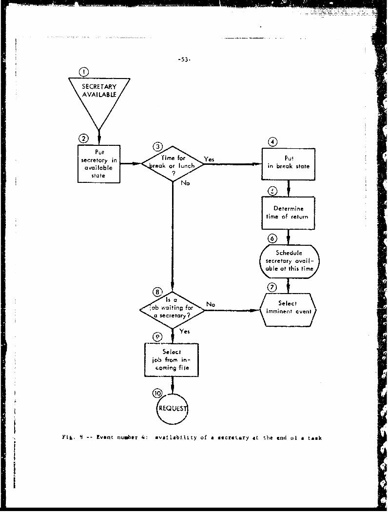
-53-

SCRE TAYA VAI LABL

Put pZ

aoilob le reak or lunch in break state

r,40 rDeterminetime of return

Schedulesecretory avail-able at this time

[obaing a- NoSeec

Yi~ ~ - Een n~er4 vaLiityofa secretarya h n fats

Seec

jo ro ncoigfil

The Program -4

PREAMBLENORMALLY MODE IS INTEGER"DECLARATION OF STATIC SYSTEM STRUCTURE

THE SYSTEM OWJNS A REQUEST .FILEPERMIANENT MITIES ....

EVERY EXECUTIVE HAS A POSITION AND A STATEEVIERY SECRETrARY HAS A STATUSEVERY TASK.TYPE HAS A TASK.TIME, A NEED, AND

AN INDUCE . PROBABILITYEVERY SECRETZARY, TASK.TYPE HAS A SKILL.FACTOR

DEFINE TASK.TTME, INDUCE.PROBABILITY ANDSKILL.FACTOR AS REAL VARIABLES

TEMPORARY ENTITIES ....EVERY TASK HAS A WHO, A WHAT AND A DELAY.TYPE

AND MAY BELONG TO THE REQUEST.FILE''DECLARATION OF DYNAMIC SYSTEM STRUCTUREEVENT NOTICES ..

EVERY REQUEST-HAS AN EXEC AND A CLASSEVERY REVIEW HAS AN EX AND A SECEVERY EXECUTIVE.AVAILABLE HAS AN EkiEVERY SECRETARY.AVAILABLE HAS A SECI

EXTER.NAL EVENTS ARE REQUEST AND END.OF.SIMULATIONBREAK REVIEW TIES BY HIGH EX THEN BY LOW SECPRIORITY G-RDER ''OF Z'vWENTS'' IS REQUEST, REVIEW, SECRETARY.AVAILABLE,

EXECUTIVE .AVAILABLE AND END. OF. SIMULATION''OTHER DECLARATIONSDEFINE OFFICE.!STATUS AS AN INTEGER FUNCTIONDEFINE INDUCE .TYP'E, SECRETARY.REQUIRED .CLASS AND

SUM .REQUESTS A S INTEGER VARIABLESDEFINE SATISFACTCkY AS A REAL VARIABLEDEFINE IDLE TO JIXAN 0DEFINE W~iudiiG TO MEAN 1DEFINE BREAK TO MEAN 2''DATA COLLECTION AND ANALtYSIS DECLARATIONS

ACCUMULATE AVG .BACKLOG AS THE MEAN ANDSTD.BCKLOG AS THE STD.iJEV OF N.IIEQUEST.FILE,

ACCUMUATE STATE.EST(O TO 2 BY 1)AS THE HISTOGRAMOF STATE

ACCUMULATE STATUS.EST(O TO 2 BY 1)AS THE HISTOGRAMOF STATUS

END

-55-

MAIN ''THIS ROUTINE CONTROLS THE SI.MULATION EXPERIMENT

'INITIALIZE' CALL INITIALIZATION ''TO ESTABLISH THE INITIAL SYSTEM STATE

START SIMULATION ''BY SELECTING THE FIRST EVENT

''WHEN SIMULATION RUN IS ENDED CONTROL PASSES HERE

IF DATA IS ENDED, STOP

OTHERWISE...''GET SET FOR ANOTHER RUN

UNTIL REQUEST.FILE IS EMPTY, DO

REMOVE THE FIRST TASK FROM THE REQUEST.FILE

DESTROY THE TASK

LOOP

GO INITIALIZE ''FOR THE NEXT EXPERIMENT

END

ROUTINE FOR INITIALIZATIONREAD N.EXECUTIVE CREATE EACH EXECUTIVE

READ N.SECRETARY CREATE EACH SECRETARY

READ N.TASK.TYPE CREATE EACH TASK.TYPE

FOR EACH EXECUTIVE, DO READ POSITION(EXECUTIVE) AND

STATE(EXECUTIVE) RESET TOTALS OF STATE LOOPFOR EACH SECRETARY, DO

READ STATUS(SECRETARY) RESET TOTALS OF STATUS

ALSO FOR EACH TASK.TYPE, READ SKILL.FACTOR(SECRETARY, TASK.TYPE),TASK .TIME(TASK .TYPE), NEED(TASK .TYPE),

INDUCE. PROBABILITY(TASK.TYPE)

LOOPREAD INDUCE.TYPE, SECRETARY.REQUIRED.CLASS AND SATISFACTORY

RESET TOTALS OF N.REQUEST.FILE

END

" ,,..UE::_JEST GIVEN EXEC AND CLASS iAVIN i IhE - VZ- ''I*.ADD 1 TO SUM.REQUESTS ''COUNT NUMBER OF TASK REQUESTSIF REQUEST IS EXTERNAL, READ EXEC AND CLASS ''FROM A DATA CARD

REGARDLESS...''PROCESS THE REQUESTIF OFFICE. STATUS-WORKING,

NOW INITIATE.TASK GIVING EXEC AND CLASS GO AHEADOTHERWISE...''FILE THE REQUEST UNTIL THE BREAK IS OVER

CREATE A TASK ''TO ACT AS A MEMOLET WHO-EXEC ''RECORD WHO THE REQUEST WAS FOR

LET WHAT-CLASS ''RECORD THE TYPE OF TASKLET DELAY.TYPE-O ''RECORD THAT THE MEMO REPRESENTS A REQUEST''RECEIVED DL'ING A BREAK PERIOD

FILE THE TASK IN THE REQUEST.FILE'AHEAD' DESTROY THE REQUEST

RT URN ''TO THE TIMING ROUTINE

END

-56-

ROUTINE TO INITIATE .TASK GIVEN EXECUTIVE AND CLASSDEFINE EXEC.TIME AND SEC.TIME AS REAL VARIABLESIF EXECUTIVE, "NO EXECUTIVE :',S ZEEN SPECIFIED, SELECT ONE

FOR EACH EXECUTIVE WITH STATE-IDLE AND POSITION GE NEED(CLASS),TIND THE FIRST CASE

IF 17OUND, GO TO 'SEC.TEST'ELSE...''NO EXECUTIVE AVAILABLE FOR THIS TASK

'NO.EXEC' LET D-1 ''INDICATING THE TASK IS WAITING FOR AN EXECUTIVE'NO.WORKER' CR,.!E A TASK LET WHO-0 L-"T WHAT-CLASS

kjt DELAY.TYPE-DFILE THE TASK IN THE REQUEST.FILERETURN ''TO THE TIMING ROUTINE

ELSE...''AN EXECUTIVE HAS BEEN REQUESTED

IF STATE-,-IDLE,''REQUESTED EXECUTIVE IS BUSY, LOOK FOR SUBSTITUTECALL SUBSTITUTION GIVING EXECUTIVE YIELDING EXECUTIVE

THEN IF EXECUTIVE-0, ''NO SUBSTITUTE CAN BE FOUNDGO TO NO.EXEC

ELSE ''AN EXECUTIVE IS AVAILABLE, IS A SECRETARY REQUIRED?'SEC.TEST' IF CLASS >- SECRETARY.REQUIRED.CLASS,

''A SECRETARY IS REQUIRED FOR THIS TASKPERFORM SECRETARY.SELECTION YIELDING SECRETARYIF SECRETARY-0, ''NO SECRETARY IS AVAILABLE FOR TASK

LET D-2 ''INDICATING THE TASK IS WAITING FOR A SECRETARYGO TO NO.WORKER

ELSE... "DETERMINE TIME EXECUTIVE AND SECRETARY WORKLET EXEC .TIE-EXPONENTIAL .F (TASK .TIME (CLASS), 1)LET SEC.TIME-EXEC.TIME + EXPONENTIAL.F(TASK.TIME(CLASS), l)*

SKILL .FACTOR(SECRETARY, CLASS)LET STATUS-WORKING ''SET THE SECRETARY IN THE WORKING STATESCHEDULE A REVIEW UXECUTIVE, SECRETARY) IN SEC.TIME MINUTES

REGARDLESS...

IF EXEC.TIME-O ''EXECUTIVE IS WORKING ALONE AND 14ST COMPUTE''HIS TIMELET EXEC.TIME-2*EXPONENTIAL.F(TASK.TIME(CLASS), I)

REGARDLESS...LET STATE-WORKI:G ''SET THE EXECUTIVE IN THE WORKING STATESCHEDULE AN EXECUTIVE.AVAILABLE(EXECUTIVE) IN EXEC.TIME MINUTESIF CLASS > INDUCE.TYPE, "CHECK FOR .AN INDUCED TASK

CREATE A REQUEST CALLED INDUCEDLET EXEC (INDUCED)-EXECUTIVELET CLASS(INDUCEI-,CLASS- 1SCHEDULE THE REQUEST CALLED INDUCED IN UNIFORM.F(0.0,1.0, 1) HOURS

REGARDLESSRETURN "TO THE TIMING ROUTINEEND

..57..

ROUTINE SUBSTITUTION GIVEN EXEC YIELDING EXECI''FIND THE FIRST IDLE EXECUTIVE WITH AT LEAST THi SAME RANKFOR EACH EXECUTIVE WITH STATE-IDLE AND POSITION >

POSITION(EXEC), FIND ':XECl-THE FIRST EXECUTIVEIF NONE, LET EXECImOREGARDLESS RETURN ''TO THE CALLING PROGRAMEND

ROUTINE FOR SECRETARY.SELECTION YIELDING SECRETARY''FIND THE FIRST IDLE SECRETARYFOR EACH SECRETARY WITH STATUS-IDLE, FIND THE FIRST CASEIF NONE, LET SECRETARY-flREGARDLESS RETURN ''TO THE CALLING PROGRAMEND

EVENT REVIEW GIVEN EXECUTIVE AND SECRETARYIF STATE-,-IDLE, ''EXECUTIVE BUSY, CANNOT REVIEW JOB

CREATE A TASKLET WHO-EXECUTIVE LET W HAT=SECRETARYLET DELAY.TYPE-3 ''INDICATING A DELAYED REVIEWFILE THE TASK IN THE REQUEST.FILEDESTROY THE REVIEWGO RETURN

ELSE...' 'EXECUTIVE REVIEWS SECRETARY'S WORKIF RANDOM.F(2) LE SATISFACTORY,

''TASK HAS BEEN PERFORMED SATISFACTORILYSCHEDULE A SECRETARY.AVAILABLE(SECRETARY) NOWGO RETURN

ELSE...''TASK MUST BE CORRECTEDRESCHEDULL id{IS REVIEW IN 13 MINUTES

'RETURN' RETURN ''TO THE TIMING ROUTINEEND

-58-

EVENT EXECUTIVE.AVAILABLE GIVEN EXECUTIVE

LET STATE-IDLE ''PUT EXECUTIVE IN THE IDLE STATEIF OFFICE.STATUS -- WORKING,

''A BREAK PERIOD IS IN PROGRESSLET STATE-BRE.AK ''PUT THE EXECUTIVE IN THE BREAK STATERESCHEDULE THIS EXECUTIVE.AVAILABLE AT TRUJW.F(TIME.V)+

GO RETURNOTHERWISE...''EXECUTIVE iS FREE TO WORK ON BACKLOGGED TASKSIF REQUEST.FILE IS EMPTY, GO RETURNELSE...' 'FIND TASKS NEEDING EXECUTIVE ATTENTIONFOR EACH TASK Ill THE REQUEST.FILE WITH DELAY.TYPE-, -2

FIND THE FIRST CASE ''NOT WAITING FOR A SECRETAR-iIF NONE, GO RETURN "NO BACKLOGGED EXECUTT"- JOBSELSE...''EXAMPLE TASK

REMOVE THE TASK FROM THE REQUEST .FILEIF DELAY.TYPE-0 OR DELAY.TYPE-I, ''WAIT IS TO START A NEW TASK

CREATE A REQUEST SUB'TRACf 1 FROH SUiH.REQUESTSSCHEDULE THE REQUEST(WHO, WHAT)NOWGO AHEAD

ELSE ''TASK IS A SECRETARY REVIEW, THE VARIABLE "WHAT"''IS USED FOR THE SECRETARY IDENTIFICATION

SCHEDULE A REVIEW(Wl;O, WHAT)NEXT'AH EAD' DESTROY THIS TASK'RETURN' RETURN ''TO TH-E ROUTINE

END

EVENT SECRETARY.AVAILABLE GIVEN SECRETARYLET STATUS-IDLE ''PUT SECRETARY IN THE IDLE STATEIF OFFICE.STATUS -, -WORKING,

''A BREAK PERIOD IS IN FROGRESSLET STATUS-BREAK "PUT THE SECRETARY IN THE BREAK STATESCHEDULE THIS SECRETARY.AVAILABLE AT TRUNC.F(TIME.V)+1GO RETURN

ELSE...''SECRETARY IS FREE TO WORK ON BACKLOGGED TASKSIF THE REQUEST.FILE IS EMPTY, GO RETURNELSE...''FIND TASKS NEEDING SECRETARIAL ATTENTIONFOR EACH TASK IN THE REQUEST.FILE WITH DELAY.TYPE-2,

FIND THE FIRST CASEIF NONE, GO RETURN ''NO TASKS WAITING FOR A SECRETARYELSE...REMOVE THE TASK FROM THE REQUEST.FILECREATE A REQUEST SUBTRACT I FROM SUM.REQUESTSSCHEDULE THE REQUEST(WHO, WHAT)NOWDESTROY THIS TASK

'RETURN' RETURN ''TO THE TIMING ROUTINEEND

-59-

EVENT END .OF .SIMITTJATI3CNOW REiORTFOR I-I TO EVENTS.V, ''EMFrY THE EVENTS LISTUNTIL EV.S(I) IS EMPTY, DO

REMOVE THE FIRST J FROM EV.S(I)GO TO REQ OR REV OR SEC Oft EXEC PER I'REQ' DESTROY THE REQUEST CALLED J

GO LOOP'REV' DESTROY THE REVIEW CALLED J

GO LOOP'SEC' DESTROY THE SECRETARY.AVAILABLE CALLED J

GO LOOP'EXEC' DESTROY THE EXECUTIVE.AVAILABLE CALLED J

'LOOP' LOOPRETURN ''TO THE TIMING ROUTINEEND

ROUTINE FOR OFFICE.STATUSDEFINE T AS A REAL VARIABLELET T-MOD.F(TIME.V,24)IF 12 - HOUR.F(TIME.V) OR 10.75 < T < 11 OR

15.75 < T < 16, RETURN WITH 0 ''INDICATING BREAK IN PROGRESSELSE RETURN WITH 1 ''INDICATING OFFICE NOW WORKINGEND

ROUTINE REPORTSTART NEW PAGEPRINT 2 LINES WITH AVG.BACKLOG AND STD.BACKLOG THUS

AVERAGE BACKLOG IS **.** TASKSSTD.DEV IS **

SKIP 3 OUTPUT LINESBEGIN REPORTBEGIN HEADINGPRINT 2 LINES THUS

ANALYSIS OF EXECUTIVE STATUSIDLE WORKING BREAK

END ''HEADINGFOR EACH EXECUTIVE, PRINT 1 LINE WITH STATE.EST(EXECUTIVE,1)/

TI.!E.V - 1'TP, .-T(XECUTIVE,2)/TIME.V, STATE.EST(EXECUTIVE,3)/TIME.V AS FOLLOWS

* o** o** **

END ''REPORTSKIP 3 OUTPUT LINESBEGIN REPORTBEGIN HEADINGPRINT 2 LINES THUS

ANALYSIS OF SECRETARY STATUSIDLE WORKING BREAK

END ''HEADING

-60-

FOR EACH SECRETARY, PRINT 1 LINE WITH STATUS .EST(SECRETARY, i)/

TIME.V, STATUS.EST(SECRETARY,2)/TIME.V, STATUS.EST(SECRETA-RY,3)/TIME.V AS FOLLOWS

END ''REPORTSKIP 5 OUTPUT LINESPRINT 1 LINE WITH SUM.REQUESTS AND TIME.V LIKE THIS

***REQUESTS WERE PROCESSED IN ****. SIMULATED DAYS

RETU)V ''TO CALLING PROGRAMEND

-61-

Description of the Program

Rather than describe the SIMSCRIPT II program in detail, we dis-

cuss only those statements that highlight SPL features mentioned in

previous sections. The purpose of the examples is to show how various

languages implement gimilation programming concepts, not to describe

the languages themselves. Those who wish to understand the examples

and the languages more fully can do so by studying their respective

programming manuals.

The preamble to the subprograms that make up the SIMSCRIPT II

model declares the static system structure of the model, using the

entity-attribute-set organization framework; declares the events that

compose the dymamic structure; defines special properties of the two

structures, such as the mode of attributes, the ranking of sets, and

the priority order of events; and specifies data-collection and analysis

tasks. The preamble is a set oi global declarations that describe the

system being simulated to the SIMSCRIPT II compiler. In the case of

the data-collection and analysis statements and some debugging state-

ments not illustrated in the example, the preamble also specifies tasks

that the compiler is to perform.

The main routine provides overall simulation experiment control.

It calls on a programmer-written routine to initialize the static

system state and provide events for the timing routine that will set

Lhe model in motion. The START SIMULATION statement removes the first

scheduled event (the initialized event with the earliest event time)

from the file of scheduled events and starts the simulation by trans-

lerring program control to it.

Eventually, either by running out of data Gr by programmer action,

all events are processed, no new ones are created, and control passes

from the timing routine (represented by the START SIMULATION statement)

to the statement that follows it. If there are no more data, the

sequenc2 of experiments is terminated. If there are mare data, the

system is initialized for another run.

The two routines MAIN and INITIALIZATION illustrate the primary

features SINSCRIPI II provides for controlling simulation experiments.

-62-

In the next routine, an event named REQUEST, the features of

interest are the statements CREATE, FILE, anJ DESTROY. The CREATE

statement generates a new entity of the class TASK whenever it is

executed; this statement is SIMSCRIPT 11's way of dynamically allocating

:torage to system entities as they are needed. The DESTROY statement

takes a named entity, REQUEST in this example, and returns it to a

pool of free data storage, providing space for the subsequent creation

of additional entities. The FILE statement takes a named entity and

puts it in a set along with other entities. In this example an entity

named TASK is put in a set named REQUEST.FILE.

In the routine INITIATE.TASK, the features to note are IF and FOR

statements that perform logical tests and searches, the statistical

function EXPONENTIAL.F, and the event-scheduling statements. The IF

and FOR statements are SIMSCRIPT II's way of dealing with the common

programming problem of determining the state of objects, or of the

system itself, and selecting among objects according to stated criteria.

The statistical function indicates the way sampling is done to repre-

sent statistically varying phenomena. The last argument in the

EXPONENTIAL.F function-call selects one of ten built-in number streams;

if the argument is negative the antithetic variate of the generated

pseudorandom number is used. The SCHEDULE statements are the basic

mechanism for specifying events that are to occur in the future. When

a SCHEDULE statement is executed, an entity, called an event notice,

of a specified type is put in a time-ordered file that is ordered by

the schedule time; when the simulation clock advances to this time,

the event is executed and is said to "occur."

The event routines EXECUTIVE.AVAILABLE and SECRETARY.AVAILA.BLE

contain REMOVE statements. These statements retrieve entities from

sets.according to criteria that are either implied or specified in

the preamble. One of the functions of the preamble is to specify such

things as the relationship that entities in sets have to one another.

The REPORT routine illustrates SIMSCRIPT II's facilities for

generating reports. N,:0 output is collected, analyzed, or prir.ted

automatically by SIMSCRIPT II. Rather, the data-collection and anal-

ysis statements of the preamble and the report specification features

pictured are used to tailor reports to simulation experiment requirements.

-63-

Naturally, this brief explanation has not made the program clear

in Ali its details -- that was not its intent. Rath-r, its purpose is

to show how SIMSCRIPT 1I provides the simulation-oriented features dis-

cussed in Sec. III. All three of the following examples follow this

same patteni.

SIMULA: A PROCESS-ORIENTED LANGUAGE

This example has been taken from Chapter 13 of [13).* Its model

is similar to those used in many SPL descriptions, and aside from

terminology, structurally very similar to the SII!CRIPF" II model just

presented. The program ie quite different.

The Model

A job consists of machine groups, each containing a given number

of identical machines in parallel. The system is described from a

machine point of view, i.e., the products flowing through the system

are represented by processes that are passive data records. The

machinec opetrte on the products by remote accessing.

The products consist of orders, each for a given number of product

units of the same type. There is a fixed number of product types. For

each type there is a unique routiP3 and given processing times.

For each machine group (number g) there is a set avail[rag of

idle machines and a set cue[mxl, which is a product queue common to

the machines in this group. The products are processed one batch at

a time. A batch consists of a given number of units, which must belong

to the same order. The batch sizt depends on the product type and the

machine group.

A product queue is regarded as a queue of orders. The queue dis-

cipline is essentially first-in-first-out, the position of an order in

the queue being defined by the errival of the first unit of that order.

However, if there is less than an acceptable batch of units of a given

order waiting in the queue, i.e., if the batch size is too small as

yet, the next order is tried. The last units of an order are accepted

Courtesy of the Norwegian Computing Center.

-64-

as a batch, even if the number of units is less than the ordinary

minimum batch size. If a machine finds no acceptable batch in the

product queue, it waits until more units arrive.

Although the individual pieces of product are "units," a unit is

not treated as an individual item in the present ,odel. For a given

order and a given step, i.e., machine group, in its schedule, we define

an opart (order part) record to represent the group of units currently

involved in that step. The units are either in processing or waiting

to be processed at the corresponding machine group.

An order is represented by a collection of opart records. The

sum of units in each opart is equal to the number of units in the

order. Each opart is a member of a product queue. If a machine group

occurs more than once in the schedule of a product type, there may be

more than one opart of the same order in the product queue of that

machine group.

Among the attributes of an opart record are the following integers:

the order number, ono, the product type, the step, the number of units

waiting, nw, and the number of units in processing, p. The flow of

units in the system is effected by counting up and down the attributes

nw and np of opart records.

An opart record is generated at the time when the first batch of

units of an order arrive at a machine group. It is entered at the end

of the corresponding product queue. The opart will remain a member of

this queue until the last unit has entered processing. It will drop

out of the system when the last unit has finished processing. A

Boolean attribute last is needed to specify whether a given opart con-

tains the last units of the order involved in this step.

At a given time the units of an order may be distributed or sev-*

eral machine groups. There will be an opart record for each of them.

An opart process will reference the one at the next step, i.e.,

machine group, through an element attribute "successor." An order is

thus represented by a simple chain of opart records. The one at the

The terms "record" and "process" both refer to the data structureassociated with a particular group of units. See Lines 5-7, p. 66.

jAhead has no successor, the one at the tail has its attribute "last"

equal to true. The chain "moves" through the system by growing new

,Cads and drcpping off tails.

que I )] que k]

3 4

I t2II

machine group i machine group mcchine group k

Fig. 9 Flow of produLtS through the shop

Fi Iute 9 ihui& three consecutIve steps in the schedule of products

of a given type. A product queue conlsists of oparts (circles) connected

by vertical lines. Oparts belonging to the same order are connected by

horizontal lines. Machines are represented by squares. A dotted line

between an opart and a machine indicates a batch of units in processing.

When the batch of the third opart in que .jl] is finished, a new opart

receiving this batch will be generated and inacluded in queLk,.

The Progtramu

Thec following program fragmeiic is part of the head of & SIMULA

block describing, the above system. A machine activity is given. For

IiI-i

-66-

clarity, only statementa essential for the behavior of the model are

shown. The program is not complete. Underlined words are SIMUL.A

keywords.

1. set array que, avail Ll:nmg]; integer U;

- 2. integer procedure nextm (type, step); integer type, step,....;

3. Lea1 procedure plire (type, step); integer type, step; ....;

4. n procedure bsize (type, mg); integer type, mg; ....

5. activity opart (ono, type, step, nw, np, last, successor);

6. integer ono, type, step, nw, np;

7. Boolean last; element successor;

b. activity machine (mg); Integer mg;

9. integer batch, next; Boolean B; element X;

0. serve: X:head (que[mg]);

11. for X:-suc (X) while exist (X) do

12, inspect X when opart do

13. begin batch :-bsize (type, mg);

14, if nw < batch then begin

15. if last then batch :nw else go to no end;

16. nw :wnw - batch; np :-np + batch;

17. if last Anw - 0 then remove X);

18. activate first (availlmg]);

19. hold (batch x ptime (type, step)xuniform (0.9, 1.1, U));

20. np :- np - batch; B :- lastA nw + np - 0;

21. next :- nextm (type, step);

22. Inspect successor when apart do

23. bnLn nw :- nw + batch; last :- B end

24. othervise b successor :-

25. new opart (ono, type, step + 1, batLtL, 0, B, none);

26. include (successor, que tnet]) end;

27. activate first (avail [next]);

28. Io to serve;

29. no. end;

30. wait (avail [mg]); remove (current); uo to serve end;

I

I

Description of the Program

Line I The sets contain uparts and idle machines, respectively.

The variable U defines a pseudorandom number stream

( line 19).

Lines 2-4 The functions "nextm" and "ptime" specify the next

machine group and the current processing time for a

given product type and step in the schedule. "bsize"

determines the batch size, given the prnduct type and

machine group number. '1he three functions are left

unspecified, i.e., their programs are not shown,.

Lines 5-7 The meanings of the attributes of opart processes have

been explained in the model description. The activity,

body is a dusmy statement: an opart process is a data

record with no associated actions.

Line 8 The machine activity extends to and includes line 30.

The parameter mg is the machine group number. Machines

belonging to the same group are completely similar.

Line 9 "batch" is the size of the current batch of units,

"next" is the number of the next machine group for the

units currently being processed, the meaning of "B" is

explained below (line 20), aud "X" is used fur scanning.

Line 10 Prepare for scanning the appropriate product queue.

Select the first opart in que~mg].

Line 11 Scan. The controlled statement is itself a connection

statement (lines 12-29).

in the SIMULA nomenclature, a process is a dynamic structure of

an activity, i.e., an activity is a process prototype.

Connection" is a means of accessing local variables from out-

side the block in which they are defined. In this instance, attributes

of the oparts stored n queimg] are being referenced.

-68-

Line 12 !here is only one connection branch (lines 12-29).

Since a product queue contains only opart records,

connection must become effective. The attributes of

the connected opart are accessible inside the conner-

tion block.

Line 13 Compute the standard batch size.

Lines 14, 13 A smaller batch accepted only if the opart is at the

tail end of the chain. In this case "nw" is nonzero

(ci. line 17), and tht: utits are the last ones of the

order. Otherwise the next opait is tried by branching

to the end of the set inspection loop.

Line 16 "batch" units are transferred from the waiting state

to the in-processing staie b> reducing nw and increasing

np.

Line 17 The opart is removed from the product queue when pro-

cessing has started on the last units of the order.

Line 18 The current machine has found an acceptable batch of

units, and has updated the product queue. There may

be enough units left for another bat-h; therefore the

next available machine in this group (,g) is activated.

If there is no idle machine, the set availrmg] is empty

and the statement has no effect. See also lines 27

and 30.

Line 19 The expecteu processing t me is proportional to the

number of units in the batch. The actual processing

time is uniformly distributed in the interval + 10%,

around the expected value. The sequence of pseudo-

random drawings is determined by the initial value of

the variable U.

Line 20 Processing in finished; np is reduced. The Boolean

variable B gets the value true if and only if the last

-69-

units ot an order have now bet:n processed. In that

case the connected opart should drop off the chain at

this system time (see cotrinents to line 28). It follows

that B is always the correct (next) value of the attrib-

ute "last" of the succeeding opart (lines 23, 25).

Line 21 Compute the number of the machine group to receive 'he

current batch of units.

Line 22 The element attribute "successor" is inspected. The

coinection statement, lines 22-26, hqs two branchei.

Line 23 This is a connection block, executed if "successor"

refers o an opart. The latLer is a member of the

product queue of the next machine group. It receiv;.s

the processed batch of units, which are entered in the

waiting state. The attribute "laet" is updated. Notice

tha: the attributes referenced in this innet connection

block are those belonging to the successor to the opart

connected outside (X).

Lines 24, 25 If the connected apart (X) is at the head of the chaip,

the value of "successor" is assumed equal to none, and

otherwise branch io taken. A new opart is o-nerated,

and a reference to it is stored in "successor," The

new opart has the same "ono" and "type" as the old one,

and its "step" is one greater. It has "batch" units

In the waiting state and none in processing. Its

attribute "last" is equal Lo "B". Since the new opart

has become the head of the chain, its "successor"

should be equal to none. Noti.- that the initial

value of "last" may well be true, e.g., if the order

contains a single unit.

Line 26 The new opart is included at the end of the product

queue of the next machine group.

-70-

Line 27 The current machine has now transferced a batch ofunits to the product queue of next machine group.

Therefore the first available machine (If any) of that

group is activated, If that machine finds an accept-

able batch, it will activate the next machine in the

same group (line i,). This takes care of the case in

which the batch transferred is larger than the standard

batch size of the next machine group for this type of

product.

Line 28 The machine immediately returns to the beginning of

its operatior rule to look for another acceptable batch,

starting at the front end of the product queue. At

this point, if B is true, the connected opart is empty

of units and will not be referenced any more. We can

regard it as having dropped off the chain. It is easy

to demonstrate, however, that the opart will physically

leave the system, i.e., that its reference count is

reduced to zero. The possible stored references are:

(1) The variable X and the connection pointer "opart"

of this machine or another one of the same group. The

go to statement leads out of the connection block,

which deletes the connection pointer. X is given

another value in line 10. Any other machine referencing

this opart would have to be suspended in line 19, which

is impossible since np is zero (cf. the second state-

ment of line 16).

.2) Set membership in que[mg]. The opart must have

been removed from the queue (by this machine or another

one) since "last" is true and nw is now zero (line 17).

(3) The attribute "successor" of the opart preceding

this one in the chafn. The first opart of thin order

to enter the systems has no predecessor. Provided

that this first one drops out when i_ is empty, our

conclusion follows by induction (see below).

I

I>

Line 29 The end of the connection block and of the statement

controlled by the for clause in line 11.

Line 30 If, after having searched the entire product queue,

the machine has fcund no acceptable batch, it includes

i'self in the appropriate "avail" set and goes passive.

Its local sequence control remains within the wait

statement as long as the machine is in the passive

state. When the machine is eventually activated (by

anothei machine: line 27 or 18), i removes itself

from the "avail" set and returns to scan the productqueue. The "avail" sets at, operated ia the first-in-

first-out fashil.i%_

The mechanism for feeding orders into the system is not shown

above. This is typically done by the Main Program or by one or more"arrival" processes, which generate a pattern of orders, either spec-

ified in detail by input data, or by random drawing according to given

relative average frequencies of product types and order sizes.

An arrival pattern defined completely "at random is likely to

cause severely fluctuating product queues, if the load on the system

is near the maximum. The following is a simple way of rearranging

the input pattern so as to achieve a more uniform load. The algorithm

is particularly effective if there are different "bottle-necks" for

the different types of products.

31. activity arrival (type, mgl, pt);

32. integer type, mgl; real pt;

33. begin integer units;34. loop: selec. (units, type); id :- id + 1;

35. include (new opart (id, type, 1, units, 0, true,

none), que[mgl]);

36. activate first (avail [mglQ);

37. hold (ptxunitu); zo to loop end;

38. procedure select (n, type); valme type; inteIer n, type; ... ;

39. integer id;

-72-

Line 31 There will be one ''arlt:val" process for each product

type. "mgi" is the number of the first machine group

in the schedule of this type of proluct. "pt" is a

stipulated "average processing time" per unil., chosen

so as to obtain a wanted average throughput of units

of this type (see line 37).

Line 34 The procedure "select" should choose the size, "units,"

of the next order of the given type, e.g., by random

drawitng oL by scarching a given arrival pattern for

the next order of this type. "Id" is a nonlocal integer

variable used for numbering the orders consecutively.

Line 35 An order is entered by generating an opart record that

contains all the unitm of the order. The units are

initially in the waiting state. The order is filed

into the appropriate product queue. The set member-

ship is the only reference t. the opart stored by the

arrival process. Consequc-ntly, this opart will leave

the system when it becomes empty of units, as assumed

earlier (line 28).

Line 36 A machine in the appropriate group is notified of the

arrival of an oider.

Line 37 The next order of the same type is qci,dulvd to aiiive

after a waiting time proportional to the size of this

order, which ensures a uniform load of units (of each

type).

The "output" of units from the system, can conveniently be arranged

by routing all products to a dumay machine group at the end of the

schedule. It contains one or more "terminal machines" (not shown here),

In SIHULA, process records that are no longer needed, i.e., arenot referenced by any other process, are automatically returned to

available storage. This contrasts with the DESTROY statem-nt used bySI1SCRIPT for the same task.

-73-

which may perform observational functions such as recording the com-

pletion of orders.

The dynamic setup of the system is a separate task, since ini-

tially the Fain Program is the only process present. The Main Program

should generate (and activate) all processes that are "permanent" parts

of the system, such as machines, arrival processes, and observational

processes. The system can be started empty of products. However, a

"steady" state can be reached in a shorter time if orders (opart

records) are generated and distributed over the product queues in

suitable quantities.

Experimental results are obtained by observing and reporting the

behavior of the system. Three different classes of outputs can be

distinguished:

(1) On-line reporting. Quantities describing the current state

of the system can be printed out, e.g., with regular system

time intervals: lengths of product queues in terms of units

waiting, the total number of units in the system, the number

of idle machines in each group, etc. A more detailed on-

line reporting may be required for program debugging.

(2) Accumulated machine statistics. By observing the system

over an extended period of system time, averages, extrema,

histograms, etc., can be formed. Quantities observed can

be queue lengths, idle times, throughputs, and so on. The

accumulation of data could be performed by the machine

processes themselves.

Example. To accumulate frequency histogram of the idle

periods of different lengths for individual machines, insert

the following statements on either side of the "wait" state-

ment of line 30:

"tidle :- time" and "histo(T, H, time - tidle, I)," where

"tidle" is a local real variable, and T and H are arrays.

Tri] are real numbers that partition observed idle periods

(time - tidle) into classes according to their lengths, and

-74-

Hfi) are integers equal to the number of occurrences in

each class. The system procedure "histo" will increase H[i]

by one (the last parameter), where i is the smallest integer

such that T[i] is greater than or equal to the idle period,

"time - tidle." T and H together thus define a frequency

histogram, where TLil - T[i - I] is the width of the i'th

colurn, and Hri] is the column length.

(3) Accumulated order statistics. During the lifetime of an

opart record, the "history" of an order at a given machine

group can be accumulated and recorded in attributes of the

opart. The following are examples of data that can be found.

The arrival of the first unit of the order at this machine group

is equal to the time at which the opart is generated. The departure

time of the last unit is equal to the time at which the variable B

gets the value true (line 20 of a machine connecting the opart).

The sum of waiting times for every unit of the order in this queue

is equal to thi integral with respect to system time of the quantity

nw (which is a step function of time). The integral can be computed

by the system procedure "accum." The statements "nw :- nw + batch"

(lines 16 and 23) are replaced by "accum (anw, tnw, nw, + batch),"

where the real variables anw and tnw are additional attributes of the

opart process, with initial values zero and "time," respectively. The

procedure will update nw and accumulate the integral in anw. It is

equivalent to the statements: anw :- anw + nw x (time - tnw);

tnw :- time; nw - nw + batch.

It is worth noticing that arrival times, waiting times, etc.,

cannot in general be found for individual units, unless the units are

treated as individuals in the program. Neither can the maximum waiting

time for units in an order. The average waiting time, however, is

equal to the above time integral divided by the number of units in

the order.

The complete history of an order in the shop is the collection

of data recorded in the different oparts of the order. These data

can be written out on an external storage medium at the end of the

-75-

lifetime of each opart. That is, an output record could be written

out before line 28, whenever B is true, containing items such as the

order number, ono, the sum of waiting times, anw, the turrent system

time, etc. When the simulation has been completed, the data records

can be read back in, sorted according to order numbers, and processed

to obtain information concerning the complete order, such as the total

transit time, total waiting time, etc.

The same information can be obtained by retaining the complete

opart chain in the system until the arder is out of the shop; however,

th:s requires more memory soace. The chain can be retained by making

the arrival process include the initial opart in an auxiliary set, Ur

by having a pointer from the opart currently at the head of the chain

back to the initial one. The opart chain can be processed by the ter-

minal machine. (The order is completely through the shop at the time

when the attribute "last" of the opart in the terminal product queue

gets the value true.) In the former case the terminal machine should

also remove the appropria'te opart from the auxiliary set, in order to

get rid of the opart chain.

CSL: AN ACTIVITY-ORIENTED LANGUAGE

This example has been taken from [11]. While unlike the two

previous models, it is indicative of the kinds of models industrial

firms construct to solve practical operating problems.

The Model

This example is a simulation of the operation of a simple port,

which consists of an outer deep-water harbor and a series of berths.

Each berth can hold one large ship, which can berth only at full tide,

or three small ships, which can also move at half-tide. The tide runs

in a 12-hour sequence, out for seven hours, half-tide for an hour.

A distribution of unloading times for large ships is available

as data, and unloading times for small ships are normally distributed.

Interarrival times are negative exponentially distributed.

Courtesy of the IBM United Kingdom Data Centre.

-76-

The program is to record the waiting times of large and small

ships and the times for which the berths are empty. The purpose of

the simulation might be to study the operation as a basis for exper-

iments to find a more efficient way of scheduling the working of the

port, or to determine the effect of providing extra berthn. The

scheduling used in this model is a simple first-in first-out scheme.

-77--

The Program

PORT SIMULATION EXAMPLE PROGRAM

CONTROLCLASS TIME SHIP.1O0 BERTH.4

C DEFINE CLASSES OF 100 SHIP ; AND f+ BERTHSSET OCEAN HARBOUR LARGE SMALL FREE PART FULLSET SHIPIN(BERTH)

C DEFINE THE SETS REQUIRED, INCLUDING AN ARRAY OF ASC MANY SET' .S TIERE ARE BERTHS, SHIPLN(X) WILL HOLDC A LIST O THE NAMES OF SHIPS IN BERTH X

NAME S BINTEGER TIDE TLARGE TSMALL

TIiE CHANGE ARRIVE FINISHC DEFINE TWO NAME VARIABLES, AN INTEGER VARIABLE TOC SHOW THE STATE OF THE TIDE, AND ADDITIONAL TIMEC CELLS. ALSO 'WO INTEGERS TO HOLD TOTAL ARRIVALSC OF LARGE AND SMALL SHIPS RESPECTIVEI.Y.

HIST LARGEQ 25,2,5 SMALLQ 25,2,5 IDLE 25,2,5HIST UNLOD 20,3,5

C DEFINE THE HISTOGRAMS REQUIRED. LARGEQ HAS 25C CELLS WITH RANGE 0-4 (MIDPOINT 2) , 5-9)10-14 ETC.C UITLOD WILL CONTAIN TrE UNLOADING TIME DISTRIBUTIONC F'uR LAPGE SHIPS.

ACTIVITIESTIDES ARRVL BT1iL BTHS DBTH ENDING

SPECIFY THE LIST OF SECTORS (ACTIVITIES)END

SECTOR INITL

T.FINISH-24000T .LHANGE-7T .ARRIVE=OTIDE-O

C THIS SECTOR IS ENTERED ONLY ONCE AND SETS IrP THEC INITIAL STATE OF THE IDEL. T.FINISH REFERS TO THEC TIME AT WHICH SIMLATION IS TO FINISH, T.CHANGE TOC THE TIME AT WHICH THE TIDE NAT CHANGES AND TIDEC SHOWS TI STATE OF THE TIDE AS FOLLOWS -

C 0 TIDE OUT i HALF IN 2 TIDE FULL 3 HALF INC T.ARRIVAL SHOWS THE TIME BEFCRE THE NEXT ARRIVAL OFC A SHIP AT THE PORT.

FOR X = 1,SHIP

SnIP.X INTO OCEANFOR X = 1,BERTH

BERTH.X INTO FREET .BERTH.X-O

-78-

C INITIALLY ALL SHIPS ARE IN OCEANC AND ALL BERTHS FREE

READ (5,10) UNLODC READ IN THE DISTRIBUTION GIVEN AS DATA.10 FORMAT (14)

END

SECTOR TIDESC THIS SECTOR IS CONCERNED WITH TIDE CHANGES

r.CHANGE EQ 0C WHICH CAN ONLY OCCUR WHEN THEY ARE DUE

TIDE+lGOTO (10,20,10,30) TIDE

C CHANGE TIDE MARKER AND RESET TIME CELL FOR NEXTC CHANGE10 T.CHANGEi

GOTO 6020 T.CHANCE=3

GOTO 6030 T.CHANGE-7

TIDE=O60 DU'MMYC AND RETURN TO CONTROL SEGMENT

END

SECTOR ARRVILC THIS SECTOR IS CONCERNED WITH ARRIVALS OF SHIPS14 T.ARRIVE EQ 0C WHICH CAN ONLY OCCUR WHEN ONE IS DUE

FIND S OCEAN FIRST &15S FROM OCEAN INTO HARBOURT .S-0

C FIND THE FIRST SHIP IN THE OCEAN MOVE IT TO THEC HARBOUR AND ZERO ITS TIME. CELL

T .ARRIVE=NGEXP( 7)C SAMPLE THE TIME TO THE NEXT ARRIVAL

UNIFORM(SYSTEMSTREAM) GT 0.75 &13S INTO LARGETLARGE+1GOTO 14

13 S INTO SMALLTSMALL+lGOTO 14

C A QUARTER OF THE SHIPS ARE LARGE, OTHERS SMALL.C GO BACK TO START OF SECTOR IN CASE NEGEXP HASC GIVEN v ZERO SA.PLE15 WRITE(6,100) T ,FNISH,CLOCK

100 LINGEN

-79-

I NOT ENOUGH SHIPS IN MODEL - SIMULATION TERMINATED2 TIME LEFT **** TIME ELAPSED ****

ToFINISH - 0C IF A SHIP IS NOT FOUND IN OCEAN, WRITE MESSAGEC AND SET T.FINISH SO THAT SIMULATION CEASES INC SECTOR ENDNG.GOTO ENDNG.END

SECTOR BTHLC THIS SECTOR IS CONCERNFD WITH BERTHING LARGE SHIPS

TIDE EQ 2FIND B FREE ANYFIND S HARBOUR FIRST

S IN LARGEC THE TIDE MUST BE FULL, THERE MUST BE A FREE BERTHC AND A LARGE SHIP WAITING IN THE HARBOUR

ENTER -T.S,LARGEQC WHEN THE SHIP ENTERED THE HARBOUR irS TIME CELLC WAS SET TO ZERO. SINCE THEN IT HAS BEEN REDUCEDC AT EACH TIME ADVANCE AND SO -T.S IS THE WAITING-C TIME OF TtiE SHIP. THIS IS RECORDED IN THEC HISTOGRAM

B FROM FREE INTO FULLS FROM HARBOUR INTO SHIPIN(B)

C THE BERTH !S NOW FULL AND THE SHIP .MO.Z FROM THEC HARBOUR INTO THE BERTH

ENTER -T.B,IDLEC JUST AS -T.S SHOWED THE SHIPS WAITING TIME SO -T.BC SHOWS THE BERTH IDLE TIME

T.S-SAMPLE (UNLOD)C SAMPLE AN UNLOADING TIME FOR THE SHIP

RECYCLEc CAUSE ANOTHER PASS THROUGH THE SECTORS (BECAUSEC MORE THAN ONE SHIP $IGHT BERTH AT THE SAME TIVE)

END

SECTOR BTHSC TIj!S SECTOR IS CONCERNED WITH BERTHING SMALL SHIPSC AND IS StMULAR -0 THE PREVIOUS ONE

TIDE GE 1FIND S HARBOUR FIRST

S IN SMALLFIND B PART ANY &20

C THE SHIP IS HDVED TO A PARTLY FULL BERTH IF THEREC IS ONE

SHIPIN(B) EQ 2 &30B FROM PART INTO FULL

C IF THE BERTH ALREADY HAS TWO SHIPS IN IT, IT NOWC BECOMES FULL

GOTO 30

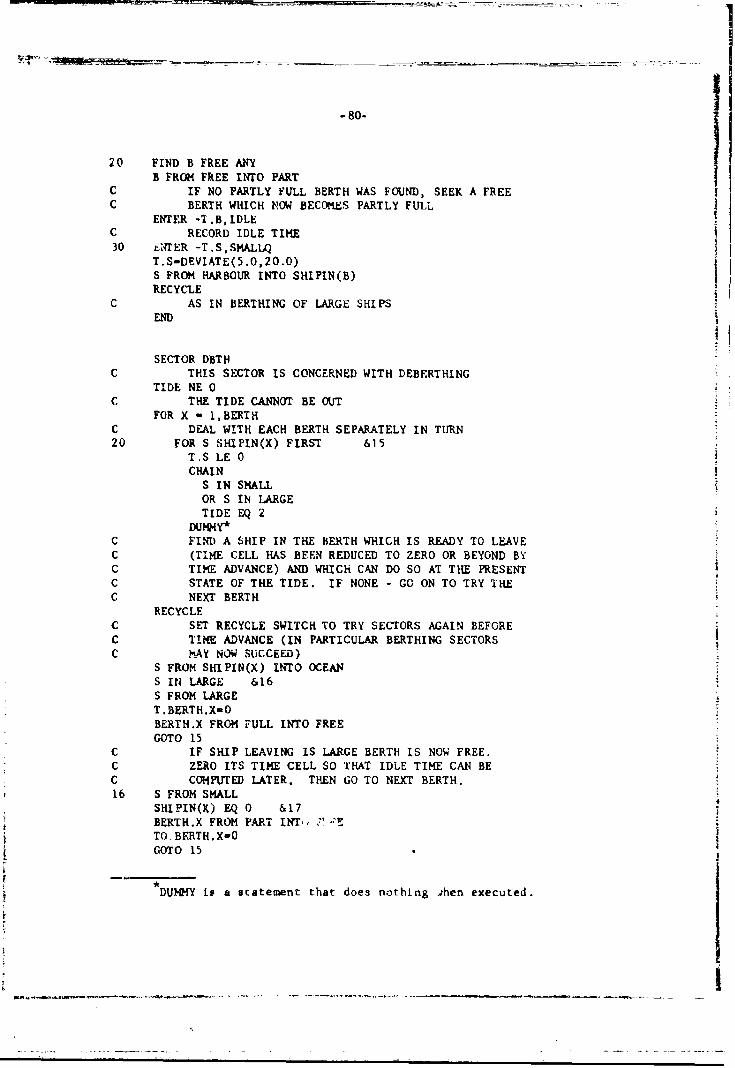
-80-

20 FIND B FREE ANYB FROM FREE INTO PART

C IF NO PARTLY FULL BERTH WAS FOUND, SEEK A FREEC BERTH WHICH POW BECOMES PARTLY FULL

ENTER -I.B, IDLEC RECORD IDLE TIME30 t-TER -T.S,SMALLQ

T.S-DEVIATE(5.0,20.0)S FROM HARBOUR INTO SHIPIN(B)RECYCLE

C AS IN BERTHING OF LARGE SHIPSEND

SECTOR DBTHC THIS SECTOR IS CONCERNED WITH DEBFRTHING

TIDE NE 0C THE TIDE CANNOT BE OUT

FOR X - 1,BERTHC DEAL WITH EACH BERTH SEPARATELY IN TURN20 FOR S SHIPIN(X) FIRST &15

T.S LE 0CHAINS IN SMALLOR S IN LARGETIDE EQ 2

DummY*C FIND A SHIP IN THE BERTH WHICH IS READY TO LEAVEC (TIME CELL HAS BEEN REDUCED TO ZERO OR BEYOND BYC TIME ADVANCE) AND WHICH CAN DO SO AT THE PRESENTC STATE OF THE TIDE. IF NONE - GO ON TO TRY THEC NEXT BERTH

RECYCLEC SET RECYCLE SWITCH TO TRY SECTORS AGAIN BEFOREC TIME ADVANCE (IN PARTICULAR BERTHING SECTORSC MAY NOW SUCCEED)

S FROM SHIPIN(X) INTO OCEANS IN LARGE &16S FROM LARGET.BERTH.X,0BERTH.X FROM FULL INTO FREEGOTO 15

C IF SHIP LEAVING IS LARGE BERTH IS NOW FREE.C ZERO ITS TIME CELL SO THAT IDLE TIME CAN BEC COMNUTED LATER. THEN GO TO NEXT BERTH.16 S FROM SMALL

SHIPIN(X) EQ 0 &17BERTH.X FROM PART INT,, tTO.BERTH.X-0GOTO 15

DUMY is a statement that does nothing hen executed.

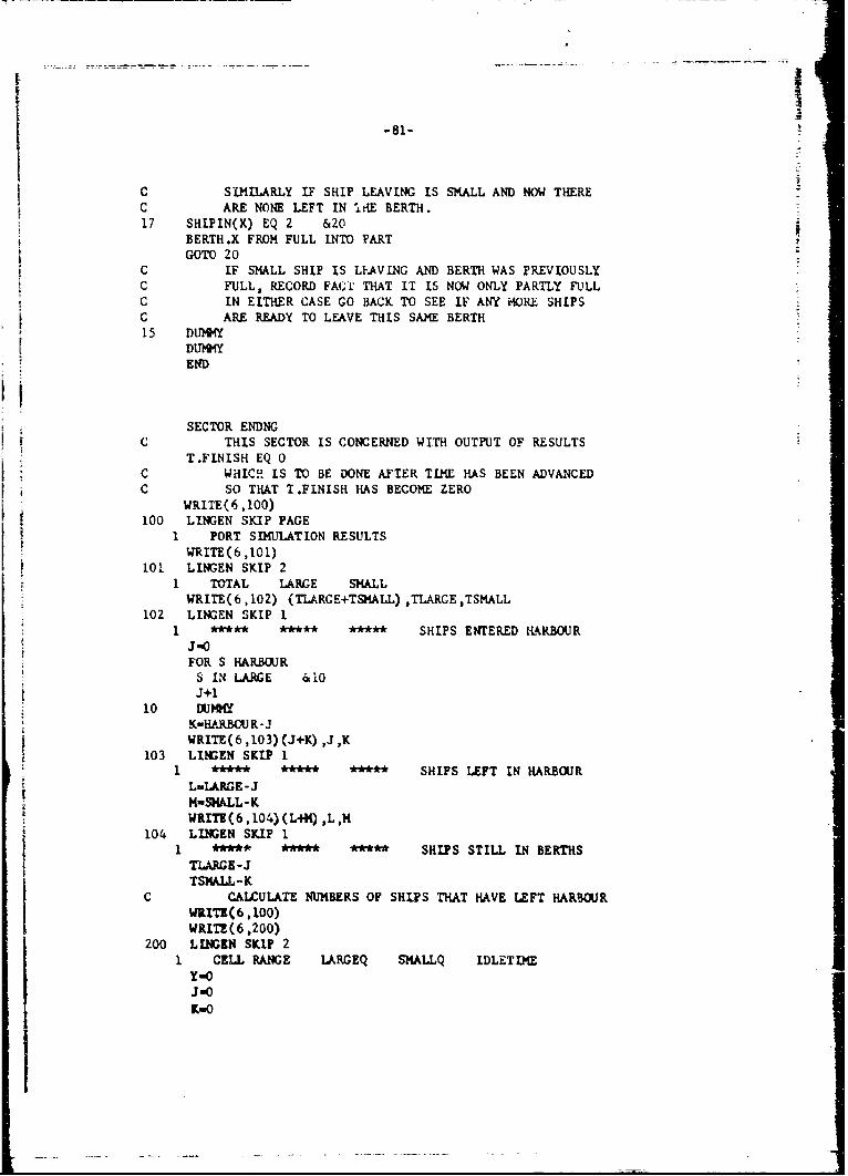
-81-

C SIMILARLY IF SHIP LEAVING IS SMALL AND NOW THEREC ARE NONE LEFT IN IRE BERTH.17 SHIPIN(X) EQ 2 &20

BERTH.X FROM FULL INTO PARTGOTO 20

C IF SMALL SHIP IS L.FAVING AND BERTH WAS PREVIOUSLYC FULL, RECORD FAC'T THAT IT IS NOW ONLY PARTLY FULLC IN EITHER CASE GO BACK TO SEE IF ANY MORE SHIPSC ARE READY TO LEAVE THIS SAME BERTH15 DUMMY

DUMMYEND

SECTOR ENDNGC THIS SECTOR IS CONCERNED WITH OUTPUT OF RESULTS

T.FINISH EQ 0C WHICH IS TO BE DONE AFTER TIME HAS BEEN ADVANCEDC SO THAT T.FINISH HAS BECOME ZEROWRITE(6 ,100)100 LINGEN SKIP PAGE

1 PORT SIMULATION RESULTS'wRITE(6,101)

101 LINGEN SKIP 2I TOTAL LARGE SMALL

WRITE(6,102) (TLARGE+TSMALL) ,TLARGE ,TSMALL

102 LINGEN SKIP I1 *** **** ***** SHIPS ENTERED HARBOUR

J-0FOR S HARBOUR

S IN LARGE &10J+l

10 Y)UMMYK-HARBOUR-JWRITE(6,103) (J+K) ,J,K

103 LINGEN SKIP 1I * *** **** SHIPS LEFT IN HARBOUR

L-LARGE-JM-SMALL-KWRITB(6,104)(L+K),L,M

104 LINGEN SKIP 11 ***** ***** ** ** SHIPS STILL IN BERTHSTLARGE -JTSMALL-K

C CALCULATE NUMBERS OF SHIPS THAT HAVE LEFT HARBOURWRITE( 6,100)WRITZ(6,200)

200 LINGEN SKIP 21 CELL RANGE IARGEQ SMALLQ IDLETIME

Y-oJ-OK-O

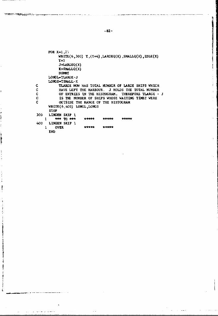
-82-

FOR X-1,2WRITE(6,300) Y ,(Y+4) ,LARCEQ(X) ,SMALLQ(X) ,WLE(X)Y+5J+IAR GEQ(X)K-SMALLQ(X)DUMMY

LONCL=TARGE -JLONGS-TSMALL- K

C TLARBE NOW HAS TOTAL NUMBER OF LARGE SHIPS WHICHC HAVE LEFT THE HARBOUR. J HOLDS THE TOTAL NUMBERC OF ENTRIES IN THE HISTOGRAM. THEREFORE TIJIRGE JC IS THE NUMBER OF SHIPS WHOSE WAITING TIMES WEREC OUTSIDE THE RANGE OF THE HISTOGRAM

WRITE(6,400) LONGL,LONGSSTOP

300 LIMEN SKIP I1 TO

400 LINGEN SKIP 11 OVER*** ***END

il

-83-

Description of the Program

The comments embedded in the program document its micro behavior

rather well. What is not obvious from the program is its macro

behavior, i.e., how activitios are controlled, initiated, and performed.

The CONTROL segment of the program has four tasks: it defines

global variables, it defines functions, it detines global FORMAT and

LINGEN statements, and it specifies activities through the sector list.

Of these, only the last is important to us now. Note that the CONTROL

segment of CSL is similar to the SIMSCRIPT II preamble.

A short discussion of how time in represented within CSL models

and how simulation is carried out should clarify the operations of

the program.

Interactions in a real system are dependent on time and the system

moves through time. It is therefore necessary to have some means of

representing time in a simulacion program. Time values are held in

variables called T-cells. T-cells may arise in two ways; they are

either defined as integer cells or arrays, or as cells attached to

their names with "T". For example, if the class of ships is defined

thus:

CLASS TIME SHIP. 100

then this serves to define entity names as above, and also 100 T-cells

addressed as T.SHIP.,..., T.SHIP.I0O. An array of integer T-cells

could be defined as

'rTT W BREAKDOWNS (10)

T-cells have all the properties of other integer cells and may par-

ticipate normally in arithmetic and tests. Their time-advancing

properties are additional.Time advancement is performed in a repeated two-stage process

as follows. Stage I scans all T-cells to find the smallest positive

nonzero value in any cell. This is regarded as the time of the next

event, or the time at %.hich an event is next able to arise in the

system. The program is now advanced to this position in time by sub-

tracting this value from all T-cells. This completes stage 1.

-84-

In stage 2 the program itself is entered. The user must specify

his program as a series of individual routines called activities, and

phase 2 consists of an attempt to obey each of the activities in turn.

Each activity describes the rules relating to the performance of one

kind of activity in the system; for example, that of unberthing a ship.

The program statements in an activity normally begin with a series

of tests to find out whether che activity can be initiated; these may

be tests on T-cells to see whether, for instance, any ships are due to

leave a berth. Following the opening tests are the statements that

actually carry out the work of the activity, e.g., arithmetic and bet-

manipulation statements.

The actual question of division of the program into activities

is governed by individual programming style. The activities must

clearly cover all possible courses of action available in the system,

but this is not the whole story. For instance, in the example program

the berthinga of large and small ships are handled as separate activ-

ities. The orders in these are largely duplicate; should they there-

fore be combined in one? This is purely a question of taste and as

such is unresolvable on logical grounds.

The structure of a CSL test can now be more fully explained. The

most frequent use of a test is at the start of an activity; under

these circumstances, if the test fails, it may be assumed that the

activity cannot be carried out.

For this reason, the customary operaiLon of computer test orders

has been changed; a test failure leads to tiansfer of control, usually

to the next activity, whereas in the case of success the next state-

ment is obeyed. To provide more detailed control of flow a statement

label may be specified; e.g.,

DATA (10) EQ 4 & 87.

In event of failure, control goes to the statemnt labeled 87.

The second phase, it will be noticed, consists of an attempt to

obey all the activities specified in the system. Apparently, this

involves auch redundant effort, as at most points in time one or two

activities oly are likely to be entered successfully end the rest

*An 6 before a number indicates that it is a statement label.

I

-63-

will be abandoned after a test or two; but a closer analysis shows

that computing time to carry out work of this kind must be expended

in any simulation programming system, whether it is carried out under

direct control of the programmer or not. It seems, therefore, most

useful to make the necessary testing explicit and under the user's

control.

When all the activities have been entered, the normal procedure

is that a return to phase I takes place and time is further advanced.

This procedure is not in itself sufficient; activities are interlinked

and the completion of orp ectivity may enable the initiation of another.

For example, the unberthing of one ship will free a berth that another

may use. The user can control this in two ways: first, by careful

choice of the order in which activities are specified, and second, by

the use of a special recycling device to cause further attempts to

obey the activities to be made.

GPSS/360: A TRANSACTION-FLOW LANGUAGE

A simple harbor model is used to illustrate GPSS. While not

identical to the CSL model, the match is close enough to provide some

feel for how the languages represent similar systems. The example is

taken from [24).*

The Model

Ships arrive at a small port with a known arrival pattern. While

in port, the ships unload some of their cargo, taking a certain amount

of time, and then proceed on their voyages. There being only one pier,

a ship must wait if it arrives while another is unloading. If several

ships are waiting, the one that arrived first will be unloaded first.

Of interest here is the total amount of time a ship will spend in port,

including the time spent waiting for the pi- to become availn,le.

Reprinted by permission from (H20-0304-l General Purpose Simula-tion System/360 Introductory User's Manual), @ (1967). and (H20-0186-1General Purpose Simulation System/360 Application Description), (1966),by International Business Machit,,es Corporation.

r

T-6

The gross behavior of the system cat, be pictured quiLe simply as:

Ships arrive at harbor in

specified arrival pattern.Arrival Average time between

artivals is 32 hours.

If pier is free, dock ship.Waiting If pier is busy, join the

line of waiting shi-s.

Begin to unload cargo.Seize Facility Unlo-ding tim is 25 + 23Hold for Process -no

Hhours. When finished,Release ship leaves pier.

Record time ship spentStatistics in harbor.

rILeave System Ship leaves harbor.

The Program

ST Unlike mo.t SPL*, GPSS has two representations, a flowchart and

a coding form language. The flowchart model of the simple harbor

system is shown in Fig. 10.

The coding form, or statement language model, is shown in Fig.

11. There is a direct correspondence between its statements and the

flowchart symbols of Fig. 10.

.1 I

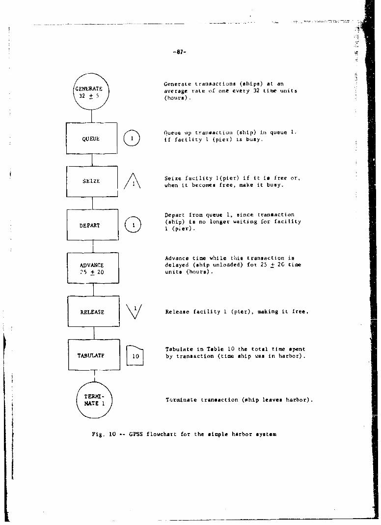
-87-

Generate transactions (ships) at anGENERATE average rate of one every 32 time units32 + 5 (hours).

Queue up trandaction (ship) in queue I.QUEUE if facility I (pier) is busy.

0

SEIZE Seize facility l(pier) if it is free or,when it becomes free, make it busy.

Depart from queue 1, since transaction

DEPART >(ship) is no longer waiting for facility1 (pier).

Advance time while this transaction is

ADVANCE delayed (ship unloaded) for 25 + 2G time

25 + 20 units (hours).

RELEASE 1 Release facility I (pier), making it free.

Tabulate in Table 10 the total time spentTAJBULATE by transaction (time ship was in harbor).

CTERMKATE 1 Tr-rinate transaction (ship leaves harbor).

Fig. 10 GPSS flowchart for the simple harbor system

I O T O M Oc'A I tOm

.. ..LI - - - 1F 11 h Ij_ i I 2,I 1AATi1

1411t*1t, cvrj Ti 4~T' ' t A.0

-+4

Fig. 11 -- PSS Harbor Model

-89-

Description of the Program

The dynamic entities in GPSS are called "transactions." These

represent the units of traffic, such as ships in this example. They

a..e "created" and "destroyed" as required during the simulation run,

and can be thought of as moving through the system causing actions to

occur. Associated with each transaction are a number of parameters,

to which the user can assign values to represeft characteristics of

the transaction. For example, a transaction representing a ship might

carry the amount of cargo it is to unload in a parameter. This number

could then be used in the simulator logic to determine how long the

unloading operation would take. Transactions can be related to one

another by placing them in groups that can be searched, scanned, and

modified.

Entities of the second class represent elements of sysLem equip-

ment that are acted upon by transactions. These include facilities,

stores, and logic switches. A facility can handle only one transaction

at a time, and could represent the pier in the example given. It

represents a potential bottleneck. A store can handle several trans-

actions concurrently, and could be used to represent a parking lot or

a typing pool. A logic switch is a two-st.te indicator that can be set

by one transaction to modify the flow of other transactions. It could

model a traffic light or the "next window" sign of a bank teller.

In order to measure system behavior, two types of statistical

entities are defined: queues and tables. Each queue maintains a

list of transactions delayed at one or more points in the system,

and keeps a record of the average number of transactions delayed and

the length of these delays. A table may be used to collcct aony sortof frequency distribution desired. These two entities provide a

major portion of the GPSS output.

The operational entities, called "blocks," constit-te the fourth

and final class. Like the blocks of a diagram, they provide the logic

of a system, instructing the transactions where to go and what to do

next. These blocks, in conjunction with the other three classes of

entities identified above, constitute the language of GPSS.

LI

-90-

To provide input for the simulation, control and definition cards

are prepared from a flowchart of the system. This constitutes the

model in GPSS language. Once the system model is loaded, the GPSS

* program generates and moves transactions from block to block according

to timing information and logical rules incorporated in the blocks

themselves. Each movement is designated to occur it 6ue pai&tiCUldL

point in time. The program automatically maintains a record of these

times, and executes the movements in their correct time sequence.

When actions cannot be performed at the originally scheduled time --

for example, when a required facility ts alreadv in isc -- processing

tempoIarily ceases for that transaction. The program automatically

maintains a status of the condition causing the delay, and as soon as

it changes, the transaction is activated again.

SUMMARY

Four different SPLs have been presented to give the reader a

helpful glance at different concepts, features, and language styles in

use today. Except for SIMULA, the examples illustrate the latestreleases of the languages.* SIMUIA 67 has been discussed in public

L16], but since no written material was available at the time this

Memorandum was written, an example of it is not included.

As these examples are small and simple, they do not illustrateall, or even necessarily the best, features of all four languages.

Some languages fare better than others in these short destinations.

The reader should bear in mind that the author's intent has not been

language instruction, but a broad-based review. No language selections

should be based on the details of this section alone. Still, it will

be a useful exercise for the reader to look back and see how the

different languages handle similar operations such as time control,

entity generation, random sampling, and set manipulation.

To be fair, it must be stated that of the fout examples presented,the one describing GPSS/360 is the least representative of the power ofits full language. The complete GPSS/360 language contains 14 entity and43 block types.

I

V. CURRENT SFL RESEARCH

SPL research is currently going on in nonprofit corporations,

universities, research organizations of computer manufacturers and

computer software companies, industria] research organizations, and

some military staff groups. With oniy a little simplification, one

czai say that this research falls ii either of two general categories:

the development of new simulation concepts, and the development of

improved simulation systems. The two are quite different, yet, since

all SPL projects seem to combine some elements of each, few people

feel they are doing strictly one or the other. Researchers developing

new concepts make advances in operating systems; experimenters devel-

oping new operating systems find new concepts arising frow their -ork.

While few projects can qualify as either pure concept development or

pure operating system design, this distinction is made in the following

discussion.

RESEARCH ON SIMLATION CONCEPTS

The 1967 IFIPS Working Conference on Simulation Languages [8]

produced several important papers on SPL design. Several of these

described modifications to existing languages, others described new

languages bated on refinements of existing concepts. The spirit of

the conference, however, was evolution rather than revolution.

Despite the fact that many SPLs are in use today, there have only

been a few instances in which a language introduced concepts signif-

icantly different from its predecessors. The languages best known torintroducing new simulation concepts are: GSP, GPSS, SIMSCRIPT, SOL,

SIMULA, and SIMPAC.

So far as we know, no completely new simulation conc.pts are

being developed today. Most language research is aimed at unifying

existing language concepts (NSS [so] is an integration of *5ICRIPT

and SIMULA with some original ideas added"), extending an accepted

IFIPS is the International Federation of Information ProcessingSocieties.

The most notable of these is a sophisticated version of theWAIT UNTIL command of SOL.

-92-

language (SIMSCRIPT I er-tends SINSCRIPT as SIM1JLA 67 extends SIMULA),

or writing a compiler fur an existing language in a widely used pro-

cedural programming language (SPL [52] is being written in PL/I and

is derived from SIKULA and SOL). A good deal of work being done

throughout the programming community on data-base concepts is finding

its way into simulation languages (e.g., SIMULA 67 and SIMSCRIPT II)

and general-purpose programing languages (reference variable exten-

sions to PL/I and ALGOL 68). Many concepts exploited in SPLs for some

time dre at present being integrated into COBOL.

There will always be room for this kind of research. Programming

being what iL is, it has no theoretical limit and there will always be

opportunities for improvements, refinements, and extensions. Until a

standard simulation programming language evolves, if that day ever

comes, people will be rewriting SPLs in new languages, discovering

new ways to do old things better, and making evolutionary changes in

concepts and implementations.

A fertile field for SPL research is language concepts. Onae area

in particular that has hardly been touched is the integration of

discrete-event and continuous-time simulation. Today, continuous-

time simulation is conducted on both analog and digital computers,

with a trend toward increased use on digital and hybrid machines [6].

The languages used for simulating continuous systems on digital com-

puters differ greatly from the SPLs we have been discussing. There

is almost no relationship between discrete-event and continuous-time

SPLs. This is a sad and hopefully short-term condition thot will be

alleviated when more research effort is expended on language integration.

A second promising area is the synthesis of modelinig languages with

procedures for performing statistical experiments and analyzing their

results. While some work has been published on efficient statistical

analysis and experimentation techniques [20], [49]. no simulation pro-

gramming languages presently contain such procedures. In part, this

is because little research has been done on identifying and developing

statistical procedures adapted especially to simulation studies. As

this area receives more attention, however, both from researchers and

practitioners, language designers will begin to consider experimentation

-93- 3

and analyses as well as modeling and true "simulation systems" will be

developed. Statisticians, language designers, simulation analysts and

computer programmers will contribute jointly to such efforts.

To speak of evolution in simulation concepts and attempt to pre-

dict the future from the past, one can be guided by these facts:

Activity- and event-oriented SPLs emerged at roughly the same

time. GSP, CSL, GPSS, and SIMSCRIPT were developed more or less in

parallel.

Process-oriented SPLs came later. SOL and SIMULA evolved from

the above languages and ALGOL.

Current research is attempting to unify and extend the activity-,

event-, and process-orientations [8].

I.terest in the statistical analyses and interpretation of

simulation results seems to be growing more rapidly each year.

It seems a good bet that research in simulation modeling concepts

will continue for some time. A great many modeling techniques still

seem forced and artificial; there is much room for improvement in

programming techniques. Topics that are well identified as needing

research attention are: decision specification -- decision tables

have not been used in SFLs; simultaneity -- parallel interactions are

currently difficult to account for; synchronous and asynchronous behav-

ior specification -- richer vocabularies for synchronizing system

processes and for executing activities asynchronously are required;

data-base definition -- we are st!!- fir from being able to specify

complex state descriptions simply and elegantly; data-base management --

efficient ways of partitioning data bases and unifying them without

complication remain to be worked out. For some solutions to these

problems, see [4], [15], and [47].

RESEARCH ON OPERATING SYSTEM AND MECHANISMS

As simulation is an experimental technique, people are always

interested in making simulation programs easier to use. The standardI

way of performing a simulation experiment today is to make a series

of experimental runs at different system parameter settings by

I

-94-

submitting a set of programs and data decks for batch processing. While

this procedure does the job, it has several serious defects: 1) pro-

h gram development and debugging is slow and painful; 2) more program

runs than necessary are usually made because of the rigidity of a scheme

requiring that a program be run completely before any information about

its behavior can be obtained and used; and 3) it is difficult to get a

feel for system dynamics by looking at a sequence of after-the-fact

system state snapahots. Systems are being designed today that assist

in each of these areas. These systems use interactive languages, time-

sharing, and graphics.

Interactive Lanauapes

The best-known interactive SPL is OPS-3 [27]. This language was

designed and impemented at M.I.T. and used successfully to demonstrate

the feasibility cf interactive modeling. Operating in a time-sharedIf

environment under the M.I.T. Compatible Time Sharing System (CTSS),

OPS-3 provides a user with on-line, interactive communication between

himself and a programming system. Using it, one can, in a single

sitting, compose a program, test and modify it, expand and embellish

it, and prepare it for subsequent production use. That interactive

languages will become standard in the future is a fact established by

OPS-3, JOSS, BASIC, RUSH, and other interactive languages. Greenberger

and Jones [28] have specified in great detail the features of an ele-

gant interactive simulation system.

Time-sharing is not mandatory for interactive man-machine dialogue,

as the above discussion might imply. At M.I.T., an SPL named SIMPLE is

being designed and programmed to operate on au, IBM 1130 computer [17].

Or such a small machine, it is economically feasible to allow one person

to have full use, even though the computer is inactive a great deal of

the time. Time-sharing allows multiple users to fully utilize a com-

puter, but it is not necessary for an interactive language.

In the future, widely used SPLa. will undoubtedly have two modes

of operation. They will be able to be used interactively to build

.JOSS is the trademark and service mark of The RAND Corporation

for its computer program and services using that program.

t IJI

a

-95- rmodels; for this either incremental compilation or interpretation will

be used. They will also be capable of efficient code generation through

optimizing compilation. This is necessary if large simulation studies

requiring lengthy experimental runs are to be made economically.

Time-Sharing

Time-sharing enters into simulation in that it makes certain things

possible, such as interactive modeling. During model construction and

testing, when programmer-program interaction is important, time-sharing

makes interaction economical. Time-sharing can also be useful during

model utilization, when production runs are made. When it is necessary

to study a model's behavior, rather than run it merely to derive steady-

state statistics, time-sharing can offer substantial benefits; when a

man can enter a program from a console, watch its performance, and either

leave it alone, stop it permanently, or stop it temporarily to adjust

some parameters and start again, a new plateau in the use of simulation

will be reached. It will then become possible for man to enter into

the exploratory and experimental process more completely and more effi-

ciently than he can in today's batch environment. For this reason,

substantial future research will be devoted to this area. The SIMPLE

language mentioned above is, in fact, designed to do this. IBM's con-

tinuous-time simulation language, CSMP, operates in this mode today L12].

Graphics

A considerable amount of sim ilat JL-oriented graphics research is

going on right now. At the Norden Division of United Aircraft, an IBM

2250 is used to modify source language GPSS programs and view their

output in graphical form [543. At The RAND Corporation, the Grail sys-

tem and the RAND Tablet are used to construct GPSS programs on-line

from hand-drawn flowcharts [30]. At M.I.T., the SIMPLE project is

using graphics for man-computer interaction during modeling and exper-

ifuentation. Papers have been written on the use of graphics in simu-

lation modeling and the use of existing graphics packages for analyzing

simulation-generated output [44).

-96-

There is little doubt that interactive modeling is carried out

better with a CRT device than with a typewriter or line printer. When

designing programs, flowcharts and other symbolic notation can be dis-

played. For analyzing performance data, graphs provide more insight

than do lists of numbers. The growing use of line-printer plotting

simulators testifies to the utility of graphic output.

Research in SPL graphics will take several directions in the

future. Graphical input is an area of great interest that is just

getting started. Graphical output is on a far firmer footing and has

had some operational success. The difficult thing about incorporating

graphics in an SPL is its ultimate dependence on graphic hardware and

software that are not properly part of a simulation language. State-

ments in SPLs that perform graphical tasks will, for a long time, be

computer-system dependent, and not independent concepts. Graphical

~research will also prosper for interactive modeling and program modi-fication. The successes and benefits claimed to date virtually insure

this.

_ _ ___ ___

-97-

VI. THE FUTURE OF SPLS

The preceding section has demonstrated that a great deal of

research remains to be done. We are far from knowing all there is to

know about simulation, both in concept and in practice. It will be

a long time before we come to a point where we wish to standardize on

a single language, and change from a dynamic era of research and

development to one of slow evolution.

The greatest challenge today lies in unifying discrete-event and

continuous-time simulation languages. Some think that this cannot be

done. Some think it should not be done. Certainly, we know little*

about how to do it.

The researcher faced with the selection of a research project in

the simulation language area does not lack alternatives. There are

still advances to be mae in modeling concepts; our ways of modeling

both static and dynamic structures are incomplete. And certainly,

the fields of interactive compilers and/or interpreters and graphics

are exciting ones and in the mainstream of modern programming research.

Today, the manager or programmer faced with the task of selecting

an SPL does not always have a clear choice. His choice will probably

be less clear in the future, as languages are drawing closer together

on many issues, but remaining apart on others. It is our hope that

this Memorandum will make some language selection choices easier and

more objective, and will provide some direction to SPL research.

A recent publication, D. A. Fahrland, "Combined Discrete-Event/Continuous Systems Simulation," SRC-68-16, Case Western ReserveUniversity Systems Research Center, July 1968, may provide the neededimpetus to initiate a constructive dialogue on this topic.

I

_ __ _

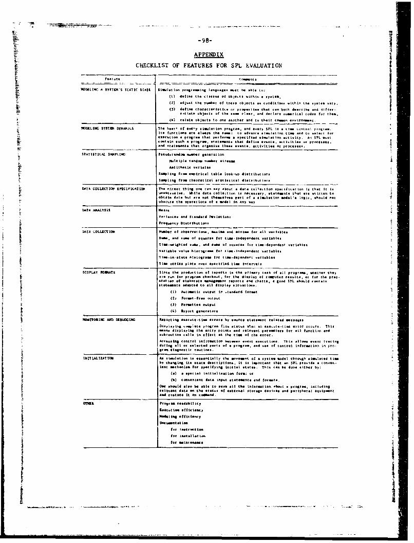
-98-

APPENDIX

CHECKLIST OF FEATURES FOR SPL EVALUATION

rest.,. m rt

IMI21LIM A SYSIDIS SIATIC STATI Simulatiton prolremelsg language. mnst hmabl ch o:

(1) define the cloesof Dobjtcte within a system,

(2) aot the nu.er of tot.on cea odttnstl h ytmvr

(2 define ch artrit or op.ie hie con bol d-so be and OlIrr atia object@ of the ae class. and decare. n-mricei codto for the.

(4) relate Ob~teo to On* another end to their comon environen.

VIiD(ELii5F SYTM~ MTAMIS lths hear, of *very simultion10 progne.. and every SPI 1. a time control programn-It@ fUPCtiLonsar Ae 4 1 YO the f800 to advnce . *tool IInn.t ie and to *elkMrt f Oraisrtto . program that p nfor a x*cifi.d sIw.at ion act ivity, A,1 SPL matlcontain such . F-r t.a stcfints that dafins events . activtoiIes or proce.104.and otai.-tns that orsaftise these events, activities or procSeas..

STATISTICAL. SWIPLIMC Pleudoranim number geneat ion

mutiple ranodom number ste.-e

Samping fro- epitil table Look-op distribut Ions

so~tling from theoreticrol stat is.icet distributitoo

DATA COLEtumvin FcIrIcATIO14 Th. nic.st thing snm can *ey about . dar nl'. to tpcfct os that it io,uabtnuetioe %Mile data collection is necessary, sattowna that are ovitten toobtain date but en. not theweive. pelt of a sim~ulation model's Ionic. should rotobscurd the operations of a sodal in any way

itkA AflALV31I Meant

Veniorceo and Stanard Ioviattona

Ptequ.ny DIeMtbut tone

LMTA LOLLCIO Number of obee.ion., macl a ed tnt-. for .11 variable.

susen and 6s~ of atuanos for tias-tndatpendent variablesTtiestghted some. and mum of squoas for ties-dependent variables

Variable value bist~grmaae for tiaw-indpndent variabies

Tims.in-tata hristograms fort tiot-dependeont vartabies

ltive mortal plots oen $pacifited tim iiervats

DISPLAY FORPAT1 $Inc* the product ion of report, is the primary task of il programs wheuther they

:7e ran for progrse checout , for the display Of roqutqd rascita, or for the prep.Cott on of *laborae* nemo reports and charts. e good S~t ebosuld noautain

stottmentoaodapted to all display situetto.q(1) Automatic output in .to.rd format

(2) Pormt-fre Output(2) porowitted Output

(46) Raport generators

PIIT111 ANDrrhi usb MgiXt Reporting eaecwi*-tion errors by coerce satement related macsagesIGloauini ,bwlt& Pcara flow. aLta wta- at n ol to rrcr 0crs. TisLmans displaying the entry points and relevant parameters for all tflnctor andsbrout int cail. io effect at the tim of the error.

Acesig control in,rmati baton. oon etxect tunas- Tis alltows event trac ingdurtog all or selected perts of a program, sad us. of controliInformAtion in pro-srma diegst i roetins..

IIPTt.AtZATI00 As simulatiopn isto eotitly the manvemnt of a eystem model through sloulated tiedby changing its state descriptions. it is important thit an SPL provide a conven.tent mechanism ion opectfykng Iitti~i stats. Thin cao be do" sither by;

(e a p*cial initutation form; or

E (b.) Convenient date input statevagnt. and foramat.

OWe absuld aiso be abie to save all the imforut ton about a prograe includingreinvn dO n the stat,. of external storage d~vlcso and peripheral *coipinnt

0 cd , 0st.r. it on taand.

orm It Program readebil icy

LOstati tofficiencyhodell~ ingefictancy

(fr imoiruaton

J for Iftataleotosh

for maneeftaee

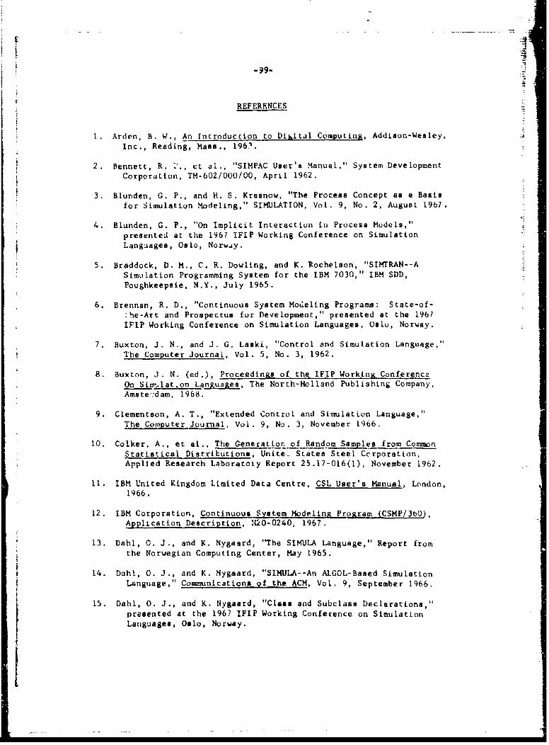
-99-

REFERENCES

1. Arden, B. W., An Introduction to Dikital Computing, Addison-Wesley,Inc., Reading, Mass., 196?.

2. Bennett, R. ,., ct al., "SIMPAC User's Manual," System DevelopmentCorporation, TM-602/O0OOO0, April 1962.

3. Blunden, G. P., and H. S. Krasnow, "The Process Concept as a Basisfor Simulation Modeling," SIMULATION, Vol. 9, No. 2, August 1967.

4. Blunden, G. P., "On Implicit Interaction in Process Models,"presented at the 1967 IFIP Working Conference on SimulationLanguages, Oslo, Norway.

5. Braddock, D. M., C. R. Dowling, and K. Rochelson, "SIMTRAN--ASimulation Programming System for the IBM 7030," IBM SDD,Poughkeepsie, N.Y., July 1965.

6. Brennan, R. D., "Continuous System Modeling Programs: State-of-:he-Art and Prospectus for Development," presented at the 1967IFIP Working Conference on Simulation Languages, Oslo, Norway.

7. Buxton, J. N., and J. G. Laski, "Control and Simulation Language,"The Computer Journal, Vol. 5, No. 3, 1962.

8. Buxton, J. N. (ed.), Proceedings of the IFIP Working ConfererceOn Singulatron Languages, The North-Holland Publishing Company,Amste-:dam, 1968.

9. Clementson, A. T., "Extended Control and Simulation Language,"The Computer Journal, Vol. 9, No. 3, November 1966.

10, Colker, A., et al., The Generation of Random Samples from CommonStatistical Distributions, Unite,. States Steel Ccrporation,Applied Research Laboratoiy Report 25.17-016(1), November 1962.

11. IBM United Kingdom Limited Data Centre, CSL User's Manual, London,1966.

12. IBM Corporation, Continuous System Modeling Program (CSMP/360),Application Description, H20-0240, 1967.

13. Dahl, 0. J., and K. Nygaard, "The SIMULA Language," Report fromthe Norwegian Computing Center, May 1965.

14. Dahl, 0. J., and K. Nygaard, "SIMULA--An ALGOL-Based SimulationLanguage," Communications of the ACM, Vol. 9, September 1966.

15. Dahl, 0. J., and K. Nygaard, "Class and Subclass Declarations,"

presented at the 1967 IFIP Working Conference on SimulationLanguages, Oslo, Norway.

-100-

16. Dah,, 0. J., B. Myhrhaug and K. Nygaard, "Some Features of the

S' flULA 67 Language," Proceedings of the Second Conference onAplications of Simulation, New York, December 2-4, i968.

17. Donovan, J. J., J. W. Alsop, and M. M. Jones, "A Graphical Facilityfor an Interactive Simulation System," Proceedings of IFIPS

Conkress, 1968.

l. l)rjift Report on the algorithmic language ALGOL b8, working paperof the IFIP Working Group on ALGOL, (Wu.2.1), February 1968.

19, Favm'lari, L., "iFORSIM IV User's Guide," SR-99, The Mitre Corpora-

tion, February 1964.

20. Fishman, G. S., and P. J. Kiviat, Digital Computer Simulation:Statisticai Considerations, The RAND Corporation, RM-5387-PR,November 1967.

21. Fishman, G. S., and P. J. Kiviat, "Tne Analysis of Simulation-

Generated Time Series," Mgmt. Sci., Vol. 13, No. 7, March 1967.

i . Galler, B. F., The Lan uage of Computers, McGraw-Hill Book Company,Inc., New York, 1962.

23. IBM, General Purpose Simulation System/360 User's Manual, H20-0326-2,

1967.

24. IBM, General Purpose Simulation System/360, Application Description,

120-0186-1, 1966.

25, Ginsberg, A. S., H. M. Markowitz, and P. M. Oldfather, Programmingby Questionnaire, The RAND Corporation, RM-4460-PR, April 1965.

26. Gordon, C., "A General Purpose SysLems Simulator," IBM Systems

Journal, Vol. 1, 1962.

2?. Greenberger, M., et al., On-Line Computation and Simulation: The

OPS-3 System, The M.I.T. Press, Cambridge, Massachusetts, 1965.

28. Greeaberger, M., and M. Jones, "On-Line, Incremental Simulation,"

presented at the 1967 IFIP Working Conference on Simulation

Languages, Oslo, Norway,

29. IBM, IBM Operating System/360. PL/I: Languale Specifications,File No. S-360-29, Form C28-6571-l, IBM Corporation, 967.

30. Haverty, J. P., Grail/GPSS, Gr-phic On-Lir. Moeling, The RAND

Corporation, P-3838, January !968.

31. Hills, P. R., "SIMON-A Computer Simulation Language in ALGOL,"

in S. H. Hollingdale (ed.), Digital Simulation in OperationalResearch, American Elsevier Publishing Co., New York, 1967.

-101-

32, Kalinichenko, L. A., "SLANG--Computer Description and Simulation-

Oriented Experimental Programming Language," presented at the

1967 IFIP Working Conference on Simulation Languages, Oslo.

Norway.

33. Karr, H. W., H. Kleine, and H. M. Markowitz, "SIMSCRIPT 1.5,"

Consolidated Analysis Centers, Inc., CACI 65-INT-l, Santa Monica,

Calif., Juae 1965.

34. Kiviat, P. J., Digital Compute- Simulation: Modeling Concepts,

The RAND Corporation, RM-5378-PR, August 1967.

35. Kiviat, P. J., "Development of Discrete Digital Simulation Languages,"

SIMULATION, Vol. 8, No. 2, February 1967.

36. Kiviat, P. J., "Development of New Digital Simulation Languages,"

Journal of Industrial Engineerln, Vol. 17, No. 11, November 1966.

37. Kiviat, P. J., "GASP--A General Activity Simulation Program,"Project No. 90.17-019(2), Applied Research Laboratory, UnitedStates Steel Corporation, Monroeville, Pa., July 1963.

38. Kiviat, P. J., Introduction to the SIMSCRIFT II Programming Lan-3 uage, The RAND Corporation, P-3314, February 1966.

39. Kiviat, P. J., R. Villanueva, and H. M. Markowitz, The SIKSCRIPTII Programming Language, The RAND Corporation, R-460-PR,

October 1968.

40 Kiviat, P. J., Simulation Language Report Generators, The RANDCorpcration, P-3349, April 1966.

41. Knuth, D. C., and J. L. McNeley, "SOL--A Symbolic Language for

General-Purpose System Simulation," IEEE Transactions on §lec-tronic Computers, August 1964.

42. Krasnow, H. S., "Dynomic Representation in Ditcrete InteractionSimulation Languages," in S. H. Hollingdale (ed.), DgtSimulation in Operational Research, American Elsevier PublishingCo., New York, 1967.

43. Kiasnow, H. S., and R. A. Merikallio, "The Past, Present nndFuture of Simulation Languages," Mt, Sci., Vol. 11, No. 2,

November 1964.

44. Lackncr, M. R., "Graphic Form for Modeling and Simulation," pre-sented at the 1967 IFIP Working Conference on Simulation Lan-

guages, Oslo, Norway.

45. Markowitz, H. M., H. W. Karr, and B. Hausner, SIMSCRT.; A Simu- :lation Prograimina Languaae, Prentice-Hall, Inc., Englewood

Cliffs, N. J., 1963.

_ - - - ~ - - - - - - . - - ~ --

-102-

46. McNeley, J. L., "Simulation Languages," SIMULATION, Vol. 9, No. 2,August 1967.

47. McNeley, J. L., "Compound Declarations," presented at the 1967.FIP Working Conference on Simulation Languages, Oslo, Norway.

48. Systems Research Group, Inc., KILITRAN Programming Manual, ReportESD-TDR-64-320, June 1964.

49. Naylor, T. H., et al., Computer Simulation Techniques, John Wileyand Sons, New York, 1966.

50. Parente, R. J., "A Language for Dynamic System Description," IBMAdvanced System Development Division Technical Report 17-180,1966.

51. Paralow, R. D., "AS: A ALGOL Simulation Language," presented atthe 1967 IFIP Working Conference on Simulation Languages, Olo,Norway.

52. Petrone, L., "On a Simulation Language Completely Defined Ontothe Programming Language PL/I," presented at the 1967 IFIPWorking Conference on Simulation Languages, Oslo, Norway.

53. Pritsker, A.A.B., and P. J. Kiviat, Simulatin with GASP II: AFORTRAN Based Simulation Language, Prentice Hall, Inc., EnglewoodCliffs, N. J. (forthcoming).

54. Reitman, J., "GPSS/360 Norden, The Unbounded and Displayed GPSS,"Proceedings of SHARE XXX, Houston, Texas, February 29, 1968.

55. Report to the CODASYL COBOL Conmittee, COBOL Extensions to HandleData Bases, prepared by Data Base Task Group, January 1968.

56. IBM, Simulation Evaluation and Analysts Language (SEAL), SyatemReference Manuel, January 1?, 1968.

57. United States Steel Corporation. Simulation Language.and LibraryISILLY), Engineering and Scientific Computer Services, February1968.

58. General Electric Company, SIMEOM User's Guide, Information SystemsOperations, TR-65-2-149010, 1964.

59. UNIVAC, SIMULA Programmer's Reference Manual, UP-7556, 1967.

60. Teichroew, D., and J. F. Lubin, 'Computer Simulation: Discussionof Techniques and Comparison of Languages," Communications of

the ACM, Vol. 9, No. 4, October 1966.

61. Tocher, K. D., "Review of Simulation Languages," OgertionalResearch Quarterly, Vol. i6, No. 2, June 1965,

-103-

62, Tocher, K. D., and D. A. Hopkins, "Handbook of the General Simula-tion Program, II," Report 118/ORD 10/TECH, United Steel Companies, ILtd, Sheffield, England, June 1964.

63. Tocher, K. D., The Art of Simulation, D. Van Nostrand Company, Inc.,

Princeton, N. J., 1963.

64. Weinert, Aria E., "A SIMSCRIPT-FORTRAN ase Study," Communicationsof the ACM, Vol. 10, No. 12, December 1967.

65. Williams, J.W.J., "The Elliott Simulator Package (ESP)," Computer

Journal, Vol. 6, No. 4, January 1964.

66. Young, Karen, "A User's Experience with Three Simulation Languages

(GPSS, SIMSCRIPT and SIMPAC)," System Development Corporation,TM-1755/000/00, 1963. I

TI

I=

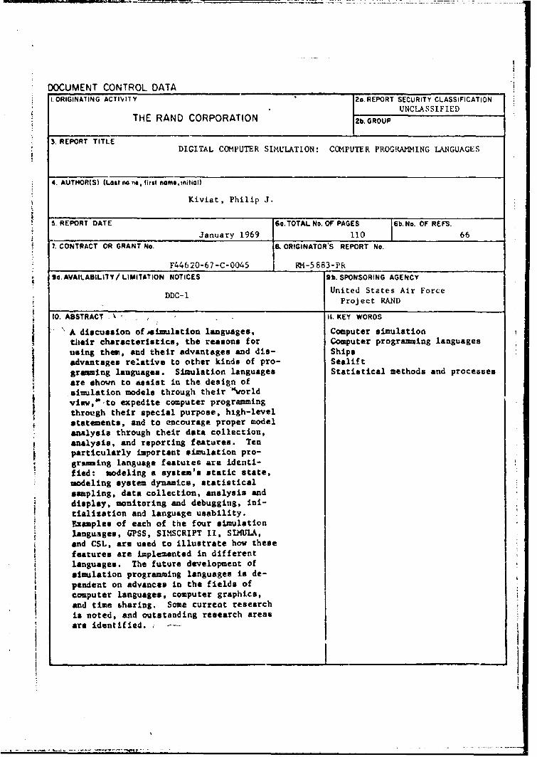
DOCUMENT CONTROL DATAI. ORIGINATING ACTIVITY 2o. REPORT SECURITY CLASSIFICATION

UNCLASSIFIEDTHE RAND CORPORATION 2b.GROUP

3. REPORT TITLEDIGITAL COMPUTER SIMULATION: COMPUTER PROGRAMMING LANGUAGES

4. AUTHOR(S) (Loaf no met, first naffle. iniliol)

Kiviat, Philip J.

5. REPORT DATE 6~o.TOTAL No. OF PAGES I~b.No. OF REFS.

January 1969 110 66

7. CONTRACT OR GRANT No. S OR!GINATOR'S REPORT No.

F44620-67-C-0045 RM-5 883-PR

go. AVAILABILITY/ LIMITATION NOTICES 9b. SPONSORING AGENCY

United States Air Force

DDC- 1 Project RAND

10. ABSTRACT ' • II. KEY WORDS

* A discussion of iimulation languages, Computer simulation

their characteristics, the reasons for Computer programming languages

using them, and their advantages and dis- Shipsadvantages relative to other kinds of pro- Sealiftgramming languages. Simulation languages Statistical methods and processesare shown to assist in the design ofsimulation models through their "worldview, ,to expedite computer programmingthrough their special purpose, high-level

* statements, and to encourage proper modelanalysis through their data collection,analysis, and reporting features. Ten

particularly important simulation pro-

gr iming language featuzes are identi-fied: modeling a system's static state,modeling system dynamics, statisticalsampling, data collection, analysis anddisplay, monitoring and debugging, ini-tialization and language usability.Examples of each of the four simulationlanguages, GPSS, SINSCRIPT I1, SIMUIA,and CSL, are used to illustrate how theme

features are implemented in differentlanguages. The future development ofsimulation programming languages is de-pendent on advances in the fields ofcomputer languages, computer graphics,and time sharing. Some current researchis noted, and outstanding research areasare identified.