computer assignment 2011.11.02

8/3/2019 Computer Assignment 2011.11.02

http://slidepdf.com/reader/full/computer-assignment-20111102 1/11

ELE 792 DSP Fall 2011

Computer Assignment: High Resolution Narrowband Spectral Analysis

Completion Date: November 31, 2011

1. Objective

In this assignment you will implement a high resolution narrow-band spectral analysis algorithm.

The algorithm uses multirate signal processing techniques together with frequency translation and

filtering to achieve high resolution spectral analysis while minimizing computational load. Such

algorithms are frequently employed in commercial FFT-based digital spectrum analyzers (such as

the Math/FFT module built in digital scopes used in the DSP Laboratory and Stanford Research

SR760 FFT Spectrum Analyzer you used in the ELE 635 Communication Systems course).

2. The ProblemIn this Section we first introduce the periodogram as a basic power spectrum estimation technique

based of DFT/FFT analysis, and then formulate its frequency resolution. This discussion will

demonstrate that high resolution spectral analysis may be computationally expensive as it will

require DFT/FFT analysis with a large number of samples.

2.1. The Periodogram

Let x[n] be discrete-time sequence acquired by sampling the analog waveform x(t) at the sampling

rate F s. Let P xx(ω) be the power spectral density (PSD) function1 of x[n]. We can estimate P xx(ω)by calculating the magnitude-squared value of the Discrete-Time Fourier Transform (DTFT) of a

finite-length segment of x[n] with N -samples after applying a window function w[n]:

P̂ xx(ω) =1

NU

N −1n=0

w[n]x[n]e− jωn2

(1)

where U is a normalization constant. When the window w[n] is the rectangular window, then

the PSD estimate is called the periodogram. If a non-rectangular window function is used, then

the estimate becomes a modified periodogram. In general, the input sequence x[n] is of much

longer duration, and therefore we can improve the periodogram estimate by first dividing x[n] into

(possibly overlapping) segments of N -samples each, calculating the periodogram corresponding

to each segment and then averaging the periodograms obtained from individual segments. Assumethat we have acquired the input so that we have access to x[n], 0 ≤ n ≤ N max. We divide x[n] into

segments of length N -samples each; let xr[n] be the rth windowed subsequence defined as:

xr[n] = w[n] x[rR + n], 0 ≤ n ≤ N − 1. (2)

If R < N , then consecutive subsequences will overlap, whereas if R = N then the subsequences

will be contiguous. Let N seg be the total number of segments that are available for processing;

1 The PSD of a stationary discrte-time random process x[n] is mathematically defined as the DTFT of rxx[m], the

autocorrelation sequence of x[n].

1 of 11



Fall 2011 ELE 792 DSP

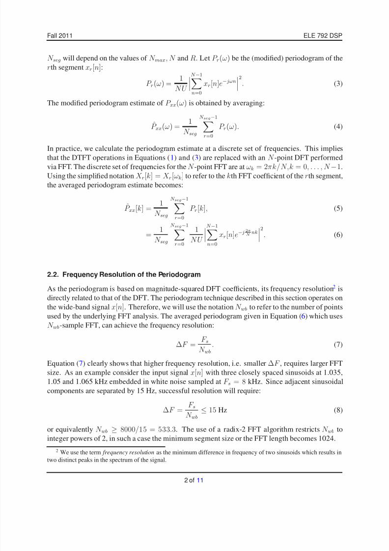
N seg will depend on the values of N max, N and R. Let P r(ω) be the (modified) periodogram of the

rth segment xr[n]:

P r(ω) =1

NU

N −1n=0

xr[n]e− jωn

2

. (3)

The modified periodogram estimate of P xx(ω) is obtained by averaging:

P̂ xx(ω) =1

N seg

N seg−1r=0

P r(ω). (4)

In practice, we calculate the periodogram estimate at a discrete set of frequencies. This implies

that the DTFT operations in Equations (1) and (3) are replaced with an N -point DFT performed

via FFT. The discrete set of frequencies for the N -point FFT are at ωk = 2πk/N,k = 0, . . . , N −1.

Using the simplified notation X r[k] = X r[ωk] to refer to the kth FFT coefficient of the rth segment,

the averaged periodogram estimate becomes:

P̂ xx[k] =1

N seg

N seg−1r=0

P r[k], (5)

=1

N seg

N seg−1r=0

1

NU

N −1n=0

xr[n]e− j2πN nk2

. (6)

2.2. Frequency Resolution of the Periodogram

As the periodogram is based on magnitude-squared DFT coefficients, its frequency resolution2

isdirectly related to that of the DFT. The periodogram technique described in this section operates on

the wide-band signal x[n]. Therefore, we will use the notation N wb to refer to the number of points

used by the underlying FFT analysis. The averaged periodogram given in Equation (6) which uses

N wb-sample FFT, can achieve the frequency resolution:

∆F =F s

N wb. (7)

Equation (7) clearly shows that higher frequency resolution, i.e. smaller ∆F , requires larger FFT

size. As an example consider the input signal x[n] with three closely spaced sinusoids at 1.035,

1.05 and 1.065 kHz embedded in white noise sampled at F s

= 8 kHz. Since adjacent sinusoidal

components are separated by 15 Hz, successful resolution will require:

∆F =F s

N wb≤ 15 Hz (8)

or equivalently N wb ≥ 8000/15 = 533.3. The use of a radix-2 FFT algorithm restricts N wb to

integer powers of 2, in such a case the minimum segment size or the FFT length becomes 1024.

2 We use the term frequency resolution as the minimum difference in frequency of two sinusoids which results in

two distinct peaks in the spectrum of the signal.

2 of 11




Figure 1: PSD estimates of x[n] based on (a) N wb = 256, (b) same but zoomed into the frequency band

[0.5, 1.5] kHz, (c) N wb = 2048, (d) same but zoomed into the frequency band [0.5, 1.5].

3 of 11




The spectrum shown in Figure (1a) is based on periodogram analysis with N = 256. Figure

(1b) which zooms into the frequency band of interest [0.5, 1.5] kHz, clearly demonstrates that this

analysis is not capable to resolve the frequency components present in x[n] (the choice N = 256corresponds to ∆F ≈ 32 which is greater than 15 Hz required for full resolution). On the other

hand, the periodogram shown in Figure (1c) and its zoomed version shown in Figure (1d) arebased on 2048-point DFT analysis. As demonstrated by Equation (8) the periodogram can now

successfully resolve the three closely-spaced sinusoids.

3. The Algorithm: High Resolution Narrow-band Spectral Analysis

The use of periodogram analysis based on long DFT sequences can achieve high frequency reso-

lution but is computationally expensive. However, in many applications such as sonar, radar and

biomedical engineering, the signal of interest may occupy only a narrow frequency band within

the spectrum of the acquired signal. In such cases, direct use of the FFT requires significant and

yet unnecessarily high computational load. As Equation (7) demonstrates, we can improve the

frequency resolution either by increasing N wb, the length of the DFT sequences, or by decreasingthe sampling rate. In particular, we can use multirate signal processing techniques to reduce the

sampling rate of the signal that will be commensurate with the bandwidth of the frequency band of

interest that is only a fraction of the full bandwidth of the signal. We now introduce such a high-

resolution narrow-band spectral analysis technique that can achieve high frequency resolution with

reduced computational effort.

The high resolution narrow-band spectral analysis (HRNBSA) algorithm operates on frequency-

translation and filtering operations to isolate the frequency band of interest and to translate it down

to baseband frequencies. The isolated signal is than decimated to reduce its sampling rate before

an FFT analysis is applied. Figure (2) shows the block diagram of the HRNBSA algorithm.

Spectral EstimationDecimation by M

x[n]

c[n] = e−jωcn

xc[n] xf [n] xd[n]

H (ejω ) ↓ M N nb-point

FFT| . |2

SpectrumDisplay

Figure 2: High Resolution Narrow-band Spectral Analysis algorithm.

The individual steps of the HRNBSA algorithm are as follows.

• Frequency Translation: The first step of the HRNBSA algorithm is frequency translation.

Let the frequency band of interest be [F 1, F 2] with 0 < F 1 < F 2 < F s/2, such that the

4 of 11




frequency of the complex exponential sequence c[n] equals F c = (F 2 − F 1)/2, and let

wc = 2πF c/F s. Using the complex exponential sequence c[n] we generate xc[n] as:

xc[n] = x[n] c[n], (9)

= x[n] e− j2πωcn

. (10)

Mixing x[n] with c[n] results in a frequency translation such that:

X c(e jω) = X ( e j(ω+ωc) ), (11)

where X (e jω) and X c(e jω) are the DTFTs of x[n] and xc[n], respectively.

• Decimation–Filtering: The second step of the HSNBSA algorithm is decimation which

starts with lowpass filtering the frequency-translated signal xc[n] to limit is bandwidth before

downsampling. Observe that for decimation by M , the passband3 of the lowpass filter is set

at F s/2M . Let xf [n] be the output of the lowpass filter. As a result of the mixing and

filtering operations, the signal xf [n] includes all frequency components in the frequency

band of interest [F 1, F 2] shifted to baseband frequencies.

• Decimation–Downsampling: The final stage of the decimation operation is downsampling

the lowpass filtered signal xf [n] by M. We downsample the signal by retaining every M th

sample of the lowpass filtered signal. Downsampling by M shortens the time sequence by

M and expands the spectrum of xf [n] by M such that:

X d(e jω) =1

M

M −1i=0

X f (e j(ω/M −2πi/M )). (12)

The decimated signal xd[n] is then fed into an FFT (or any other spectral estimation) routine

to perform spectral analysis.

Note: The spectral estimation operations (FFT followed by magnitude-squared coefficient compu-

tation) shown in Figure (2) present an implementation where the entire decimated signal xd[n] is

processed as a single block. In practice, we segment xd[n] into (possibly overlapping) N nb-sample

long subsequences, and then process each subsequence individually. The periodogram estimates

obtained from individual blocks are then averaged. This is the same approach used by the averaged

periodogram spectral estimation technique presented in Section 2.1

Equation (7) shows that the frequency resolution of the wide-band periodogram algorithmbased on N wb-point FFT analysis is F s/N wb where F s is the sampling rate of the wide-band signal

x[n]. On the other hand, the frequency resolution that the HRNBSA algorithm can achieve will

be based on the sampling rate of the decimated signal xd[n] namely F ′s = F s/M where M is the

decimation factor. Therefore, the frequency resolution of the HRNBSA algorithm based on an

N nb-point FFT analysis equals:

∆F ′ =F ′s

N nb, (13)

3 In Matlab the passband is specified as 1/M as Matlab uses the normalized frequency 1 to represent F s/2.

5 of 11




Assume that we want both the wide-band and the narrow-band spectral analyses to achieve the

same frequency resolution, i.e., ∆F = ∆F ′. This can be achieved by using a smaller FFT size. In

particular, the required number of points in the narrow-band spectral analysis becomes:

N nb = N wbM . (14)

Hence the HRNBSA algorithm results in an M -fold reduction in the FFT size—alternatively, if we

let N wb = N nb, we can achieve an M -fold increase in frequency resolution using the HRNBSA

algorithm.

To demonstrate the effectiveness of the HRNDSA algorithm let us consider the same wide-band

signal x[n] used to generate the spectral plots shown in Figure (1). Assume that the frequency band

of interest is [0.5, 1.5] kHz such that F c = 1 kHz. While the bandwidth of the frequency band of

interest is 1 kHz, the effective bandwidth of xc[n], the signal obtained by mixing the wide-band

signal x[n] with c[n], will only be 0.5 kHz, as the original frequency band of interest occupies the[−0.5, 0.5] kHz band after frequency translation. In view of the the bandwidth of the wide-band

signal x[n] being 4 kHz, the HRNBSA algorithm will use the decimation factor M = 8 = 4/0.5.

We can make a number of important observations about the HRNBSA algorithm from the PSD

functions shown in Figure (3).

• The PSD functions of the frequency translated signal xc[n] and the filtered signal xf [n] (Fig-

ures (3b) and (3d), respectively) do not have even symmetry as both signals are complex-

valued due to mixing with the complex exponential sequence c[n].

• All elements in the PSD function of xf [n] shown in Figure (3d) carry non-redundant in-

formation. This is in contrast to a real-valued signal whose PSD function would be even

symmetric and hence only the spectral components over the positive (or negative) frequency

axis would provide unique information.

• The PSD function of the decimated signal xd[n] shown in Figure (3e) demonstrates the spec-

tral expansion effect of the downsampling operation formulated in Equation (12).

• The periodogram used to estimate the PSD function of the decimated signal shown in Figure

(3e) is based on an FFT analysis with N nb = 256. Its frequency resolution is comparable

to the frequency resolution of the spectrum of the wide-band signal obtained from an FFTanalysis with N wb = 2048 shown in Figure (1c) and (1d). This comparison demonstrates

that the HRNBSA can achieve the same resolution as the wide-band spectral analysis using

FFT analysis with one-eighth points (N nb = 256 vs. N wb = 2048).

• Proper interpretation of frequency values from Figure (3e) requires that we take into account

the frequency translation resulting from mixing the input sequence with c[n]. Therefore, the

frequency origin in Figure (3e) actually corresponds to F c = 1 kHz.

6 of 11




Figure 3: PSD functions of signals generated by the HRNBSA algorithm: (a) |X (e jω )|2, the PSD function

of the wide-band input signal x[n], (b) |X c(e jω)|2, the PSD function of the frequency translated signal xc[n],

(c) |H (e jω )|2, the magnitude-squared frequency response of the lowpass filter used by the decimator, (d)

|X f (e jω )|2, the PSD function of the lowpass filtered signal xf [n], (e) |X d[k]|

2, the PSD function of the

decimated signal xd[n] generated by 256-sample FFT analysis.

7 of 11




4. The Assignment: What is to be done?

Write a Matlab function hrnbsa.m that will implement the HRNBSA algorithm as described in

Equations (1)–(8) given above. The call to the hrnbsa.m function should be in the form:

[ P nb, f nb ] = hrnbsa( Data In, Fs, [F1,F2], DeltaF );

Input Variables and Parameters:

Data In:

N max-sample long one-dimensional input sequence x[n]. In particular, Data In is a real-

valued column vector of dimension N max × 1. As an input signal (and for testing your

implementation of the HRNBSA algorithm) you can use the function textgen.m to gen-

erate a test signal with closely spaced sinusoids. For further information on this function,

see the Discussion section below. It is recommended that you use N max = 214.

Fs:

Sampling rate of the input signal Data In.

[F1,F2]:

Frequency band of interest such that 0 < F1 < F2 < Fs /2.

DeltaF:

Desired frequency resolution over the frequency band of interest.

Output Variables:

P nb:

The averaged periodogram estimate over the frequency band of interest as generated by the

HRNBSA algorithm. If the HRNBSA algorithm is based on N nb-sample long FFT analysis,

then the algorithm separates the decimated signal xd[n] into N nb-sample long subsequences,

computes their periodograms and then averages the periodograms. Therefore, P nb will be

a real-valued, N nb × 1 column vector such that P nb(1) will represent the averaged peri-

odogram estimate at frequency F1 and P nb(N nb) will represent the averaged periodogram

estimate “approximately” at frequency F2.

f nb:

This output variable will be the N nb-dimensional column or row vector that contains theN nb uniformly spaced frequency locations for the proper display of P nb. If F ′s = F s/M is the sampling frequency of the decimated signal and F c is the frequency of the complex

exponential sequence c[n], then:

f nb(1) = F1 · · · f nb(N nb

2) = F c · · · f nb(N nb) =

F ′s2

N nb − 2

N nb

+ F c

Observe that for large N nb, f nb(N nb) ≈ F2.

8 of 11




5. Discussion

You may find the following discussion and information helpful in developing your code.

• Input: You can generate input signals with the utility function textgen.m (available fromthe course homepage on Blackboard). For example, the Matlab command:

≫ N max = 2ˆ14;

≫ x = testgen(rand(N max,1), [10 8 12], [1035 1050 1065], 8000);

will generate the 2ˆ14×1 dimensional Matlab array x (i.e., a column vector) which con-

sists of three sinusoids at frequencies 1.035, 1.05 and 1.065 kHz with respective amplitudes

10, 8 and 12 embedded in white noise sampled at F s = 8 kHz.

• Block size N nb: Assume that you have access to only radix-2 FFT algorithm which requires

that the block size will be an integer power of 2. Hence, in your code let N nb = 2k

, wherek ∈ Z +. While testing your code, you may note that choosing the block size for the FFT

analysis at the theoretical limit as discussed in Section 2.2 may not result in a PSD estimate

with sufficient frequency resolution. Therefore, it is recommended that you choose a block

size that is twice as long. For example, if your analysis shows that you need a block size

with a minimum of 72 elements, you would normally choose N nb = 128 = 27 > 72; instead,

use N nb = 256. For frequency components that are well separated doubling the block size

may not be necessary; however, closely spaced frequency components particularly in the

presence of noise will require the extra resolution provided by the increased block size.

• Decimation: For the decimation stage within the HRNBSA algorithm you can use the Mat-

lab function decimate.m which includes both the lowpass filtering and the downsamplingoperations. If you decide to use decimate, choose the FIR filter option with filter order

set to 100. At the Matlab prompt type help decimate or doc decimate for further

information on how you can use this function.

Of course, you can also write your own decimator code which will consist of a lowpass filter

(the Matlab function fir1 is easy too use) and downsampler (very easy to implement). This

approach allows access to the signal at the filter output.

Extra Credit 1 Assume that you calculated that you need a decimation factor M to achieve

the user-specified frequency resolution over the frequency band of interest. If you are coding

the HRNBSA algorithm in Matlab, you can obviously proceed with this value of M —Matlabwill design the appropriate decimator for you. However, a digital spectrum analyzer with a

built-in HRNBSA, will not have access to Matlab and therefore cannot be as flexible. In-

stead, the spectrum analyzer may only have access to a very limited number of pre-calculated

decimation units which can be used in a modular fashion to achieve different decimation

factors. For example, processing the signal twice with a decimation-by-2 unit will result in

decimation by 4. Modify you code such that it can only use a decimation-by-2 module; thus,

your implementation of the HRNBSA algorithm will be restricted to use decimation factors

M = 2, 4, 8, . . ..

9 of 11




• Reshaping an array for processing: The decimated signal xd[n] (most likely represented

as a column or row vector in Matlab) will have to be segmented into N nb-sample blocks

so that an N nb-element FFT can be applied to each block. You can do this in a loop. But

for computational efficiency, try to utilize the array processing capabilities of Matlab. For

example, if the decimated signal xd[n] has N nbK elements, consider creating a N b×K matrixby reshaping the Matlab array that is the decimated signal. The built-in Matlab function

reshape can easily accomplish this task. If x array is the N b × K array generated by

reshaping xd[n], then the single command fft( x array, N b ) will compute the N b-point

FFT of each column, i.e., of each block.

• Displaying the spectrum over [−F s/2, F s/2]: By default the fft coefficients generated by

Matlab are located at uniformly spaced frequency bins over the frequency band [0, F s). In

this assignment, you will perform frequency translation and will work with complex-valued

signals. Therefore, you may find it more convenient to work with fft samples defined over

the frequency band [−F s/2, F s/2). Use the Matlab function fftshift.m on fft samples

before displaying the spectrum.

• Normalization: For normalization of the periodogram estimate use the factor 1/(F 0N )where F 0 is the sampling rate of the signal whose fft is calculated, and N is the FFT size.

If you are calculating the averaged periodogram, then you must also normalize using the the

number of blocks over which the periodograms are averaged.

• Extra Credit 2 Can you modify your code so that (i) successive blocks of decimated signal

samples overlap, and (ii) a user selected window function (e.g. Hamming, Hanning, etc.)

is applied to each block of samples extracted from the decimated signal before the FFT

operation. What are the effects of using overlapping blocks? What are the effects of using

different window functions?

6. Grading

• The efficiency of your code will be evaluated. You can measure the time your code requires

to complete its execution by using the built-in Matlab functions tic, toc and cputime.

Alternatively, you an use the Matlab profiler. You can access the Matlab profiler either from

the Desktop menu-item or by making a call to the profile function.

• During the course of this assignment you will write the Matlab function hrnbsa.m . This

file should be well commented. By the assignment completion deadline, submit your file

using the command:

submit ele792 comp hrnbsa.m

If during the course of this assignment you have generated additional M-files which are re-

quired for the operation of hrnbsa.m , please submit them in a similar fashion.

• Prepare a report no more than 4 pages long. This report should briefly describe the problem,

explain how you calculate the various parameters that the HRNBSA algorithm needs from

the input parameters Fs, F1, F2 and DeltaF. Provide a numerical example. The report

10 of 11




should also include a Conclusions section where you can present your conclusions regard-

ing the effectiveness of the algorithm. Format your report as a PDF file (PDF format only

please!) and submit your report as before:

submit ele792 comp myreport.pdf

where myreport.pdf is your PDF formatted report document.

• This assignment is worth 10 points (and is 10% of your total grade in the course). Successful

completion of the Extra Credit tasks may potentially earn you another 5 points (2.5 points

each).

References

1. A.V. Oppenheim and R.W. Schafer, Discrete-Time Signal Processing, 3rd Edition, Pearson

Higher Education Inc., 2010.

2. Richard G. Lyons, Understanding Digital Signal Processing, 3rd Edition, Pearson Higher

Education Inc., 2011.

11 of 11

computer assignment 2011.11.02

Documents