computer application in social work

COMPUTER APPLICATION IN SOCIAL WORK

Subject Code: MSW 33A

II - MSW III – Semester

PG DEPARTMENT OF SOCIAL WORK

Periyar Government Arts College Cuddalore-01

Prepared by

Dr. G. KUMAR, Guest Lecturer PG Department of Social Work

Periyar Government Arts College Cuddalore-01

NOVEMBER - 2020

BASIC OPERATIONS OF COMPUTER

COMPUTER

• A computer can process data, pictures, sound and graphics.

They can solve highly complicated problems quickly and

accurately. There are five basic operations of computer or

functions.

• 1) it accepts data or instructions by way of input,

2) it stores data,

3) it can process data as required by the user,

4) it gives results in the form of output, and

5) it controls all operations inside a computer.

https://ecomputernotes.com/fundamental/introduction-to-computer/what-is-computer

OPERATIONS OF COMPUTER

INPUT

• This is the process of entering data and programs

in to the computer system. You should know that

computer is an electronic machine like any other

machine which takes as inputs raw data and

performs some processing giving out processed

data. Therefore, the input unit takes data from us to

the computer in an organized manner for

processing.

CENTRAL PROCESSING UNIT (CPU)

• The ALU and the CU of a computer system are

jointly known as the central processing unit. You

may call CPU as the brain of any computer

system. It is just like brain that takes all major

decisions, makes all sorts of calculations and

directs different parts of the computer functions

by activating and controlling the operations.

ARITHMETIC LOGICAL UNIT (ALU)

• Logical Unit : After you enter data through the input device it

is stored in the primary storage unit. The actual processing of

the data and instruction are performed by Arithmetic Logical

Unit. The major operations performed by the ALU are

addition, subtraction, multiplication, division, logic and

comparison. Data is transferred to ALU from storage unit

when required. After processing the output is returned back

to storage unit for further processing or getting stored.

CONTROL UNIT (CU)

• The next component of computer is the Control Unit, which acts like

the supervisor seeing that things are done in proper fashion. Control

Unit is responsible for co ordinating various operations using time

signal. The control unit determines the sequence in which computer

programs and instructions are executed. Things like processing of

programs stored in the main memory, interpretation of the instructions

and issuing of signals for other units of the computer to execute them.

It also acts as a switch board operator when several users access the

computer simultaneously. Thereby it coordinates the activities of

computer’s peripheral equipment as they perform the input and

output.

STORAGE/ MEMORY UNIT

• The process of saving data and instructions permanently is known as

storage. This unit consists of locations or cells on which the data can be

stored. If you want to retrieve the data, the data can be retrieved from the

same unit. This unit consists of two types of memories namely,

Permanent memory and secondary memory. A permanent memory is

nothing but the semiconductor memory device available with int

computer. i.e. Hard disc. The secondary memory is the memory which

is movable and can be taken away frm the computer and can be kept

safely. Floppy disks, compact discs and memory strics are th eexamples

of secondary memory devices.

PROCESSING

• The task of performing operations like arithmetic

and logical operations is called processing. The

Central Processing Unit (CPU) takes data and

instructions from the storage unit and makes all

sorts of calculations based on the instructions

given and the type of data provided. It is then sent

back to the storage unit.

OUTPUT

• This is the process of producing results from the

data for getting useful information. Similarly the

output produced by the computer after

processing must also be kept somewhere inside

the computer before being given to you in human

readable form. Again the output is also stored

inside the computer for further processing.

FUNCTIONAL UNITS

• In order to carry out the operations mentioned in

the previous section the computer allocates the

task between its various functional units. The

computer system is divided into three separate

units for its operation.They are

THANK YOU

Device of Computer

Dr. G. Kumar

Guest Lecturer

PG Department of Social Work

Periyar Government Arts College, Cuddalore-01

What is computer device?

Device which means a collection of components which is

called device or hard ward.

Eg.

Input device -- Storage Device -- Out Device

Input device

Data

Program

Command

User Response

Keyboard

Mouse

Other input device

Touch pads,

Joystick

Light pens

Microphones

Web camera

Scanner

Bar code reader

Storage Device

A Storage device is the mechanism used to record

and retrieve items to and from a storage medium .

A storage medium is the physical material on which

the items are kept.

There are two types of storage device

1. Primary Storage device

2. Secondary storage devic e

Primary Storage Device

Random Access memory (RAM)

Read only Memory (ROM)

Secondary Storage Device

Floppy Disk

CD & DVD

Pen Drive

Memory Cards

External hard disk

Out put Device

Text

Graphics

Audio

Video

Monitor

Printer

Computer Application in Social Work

Topic : Software

Dr. G. Kumar

Guest Lecturer


Periyar Government Arts College, Cuddalore.

Dr. G. Kumar, Guest Lecturer, PG Department of Social Work, Periyar Government Arts College, Cuddalore.

What is Software?

Software is a set of instructions, data

or programs used to operate

computers and execute specific

tasks.


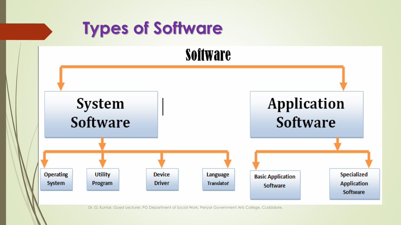
Types of Software


System Software

A set of programmes which are used to control

the system or used to improve the efficiency of the

computer is called system software.

ex.

Operating system, such DOS, Unix etc.

Utility programe – Virus scanner progamme

Language Processor, such as complier,

interpreter etc.


Operating systems Operating systems is a programme that allows different

application and various pieces of hardware such as monitor,

mouse, printer, keyboard etc. to communicate each other.

Other Operating system

Windows 95, Windows 98, windows 2000

Windows ME, Windows NT, Windows XP and Windows vista.

Windows 7, Windows 8 etc.

Cell phone Operating system

IOS, Android, windows 8.


Device Driver - Software

A device driver is a software program that controls

a particular types of (or) specific type of hardware.

Examples: Sound card driver, video card driver,

etc.


Application SoftwareA set of programs which are developed by the user

(software engineers) for day-to-day activities like

accounting is called application software.

Word Processors – Such as MS-Word, Notepad etc.

Spread Sheets – Such as MS –Excel, Lotus 1-2-3

Data bases package – Such as Foxpro, MS-access etc.

Other GUP software – Windows photo gallery, Adobe

photoshop, Adope pagemaker, Coral draw etc


Internet Browsers

Chrome

Mozilla Firefox

Internet explore and

Opera etc.


Meaning of Progamme

A computer program is a collection of instructions

that can be executed by a computer to perform

a specific task.

A computer program is usually written by

a computer programmer in a programming

language.


Computer Language It translate programming code into the machine code. So, that computer can

understand it and can process further. Computer converts the High Level Language

into Machine Language (binary language i.e, 0 and 1)

The language processors are given below-

Assembler – An assembler is a program that converts assembly language into machine

code. It takes the basic commands and operations from assembly code and converts

them into binary code that can be recognized by a specific type of processor.

Interpreter - An interpreter is a computer program that directly executes instructions written

in a programming or scripting language, without requiring them previously to have been

compiled into a machine language program.

Compiler - The language processor that reads the complete source program written in high

level language as a whole in one go and translates it into an equivalent program in

machine language is called as a Compiler.

Example: C, C++, C#, JavaIn a compiler, the source code is translated to object code

successfully if it is free of errors. The compiler specifies the errors at the end of compilation with

line numbers when there are any errors in the source code. The errors must be removed before

the compiler can successfully recompile the source code againDr. G. Kumar, Guest Lecturer, PG Department of Social Work, Periyar Government Arts College, Cuddalore.

1 | Dr. G. Kumar, Guest Lecturer, PG Department of Social Work, Periyar Government Arts College.

Unit – 2

WORD PROCESSING

Introduction

Microsoft Office is a family of client software, server software, and different services developed

by Microsoft. It was first announced by Bill Gates on 1 August 1988, at COMDEX in Las Vegas.

Initially a marketing term for an office suite (bundled set of productivity applications), the first

version of Office contained Microsoft Word, Microsoft Excel, and Microsoft PowerPoint.

What is mean by Microsoft Office?

Microsoft Office is an integrated set of software tools, software applications for Windows in

computers. MS Office includes word processing, spreadsheet, presentation. Apart from this MS-

Access (data based application, MS paint etc. and email communication programs

Office 2010 for Microsoft Windows, Office 2008 computer are the versions available as of July

2010.

Word Processing

Word processing is one of the most important activities carried out in a work place. It is a

technique used or formatting text into a more readable rom.

In early days, a manual type writer was commonly used which was later replaced by electronic

typewriter to carryout letter writing, statement preparation, report generation etc. as computers

are fast replacing most of the manual documentation work, software technically called word

processors were introduced to process text.

Microsoft word processors are application software that are used for creating, editing, transmitting,

storing and printing all kinds of documents. Word processors are applied in the field of journalism,

publishing, DTP (Desk top Publishing) etc. Thus, word processing is integral or the preparation

and presentation of documents.

Features of MS Word

MS word was developed by Microsoft incorporation. It gained popularity due to its advanced

features. Some of them, are….

a. Working with multiple documents simultaneously.

b. Auto correction of mistakes.

c. Inserting tables, charts and graphics into a document.

d. Saving and protection of documents.

e. Printing any number of copies of error free documents in desired formats.


Advantages of MS word

Microsoft Word is a great tool as typing is faster than ever,

It is easy to correct the mistakes by just hitting the backspace or delete button.

There are the templates for any type of document and mail merge from a database so that

user can easily send out the letters to multiple people at a time.

Can align the text whether at the center, right or left margins or justified takes just one

click,

Spelling and grammatical mistakes are pointed out instantly, You can correct any mistakes

which are made easily,

The bullets and numbers are done automatically and there is always an option to ask for

help.

Getting into MS Word

1. By clicking on the MS Word icon on the office toolbar -------------- click


2. By using right click on the desktop ---- the list of programe appear ---- click MS Word

– the MS word window will displayed as follows\


Components o MS Word Window

There are 7 major components designed in the ms word window which included Title bar, Menu

bar, Tool bar, Work area, Ruler, Status bar and Scroll bar.

Title bar: the title bar is displayed at the top of the window. It contains the name of the

active document on the left corner and three buttons on the right corner that is called closed

button, maximize button, and minimize button.

Menu bar: As the name suggest, the menu bar comprises of various menus. Each of the

menu contains a list of options, which can be selected.

Tool bar: The toolbar contains the collection of icons, each preforming a specific task.

These icons perform the command available under sub menu of the menu bar. There are

different toolbars available and the most frequently used toolbars are standard and

formatting.

Work area: It is a blank area where the text can be keyed in it has a blinking vertical line

called cursor that indicates where the t4ext will appear.


Ruler: Ruler controls the margins of the page. They appear on the top and left positions

of the work area.

Status Bar: The status bar is displayed at the bottom of the window. It shows the current

location of the insertion point (row, column), page number and various other modes.

Scroll bar: Scroll bars are used to scroll across the window. There are two types of scroll

bar – horizontal scroll bar and vertical scroll bar.

File Operations

A file is a collection of information stored in a computer that includes text, pictures, sounds,

movies etc. File operations included creating new files, opening an existing file, savings and

closing the active file. In MS word files are technically called documents.

Creating a new Document.

There are three ways to create a new document in MS word

1. Using file menu and choosing New option ---- click


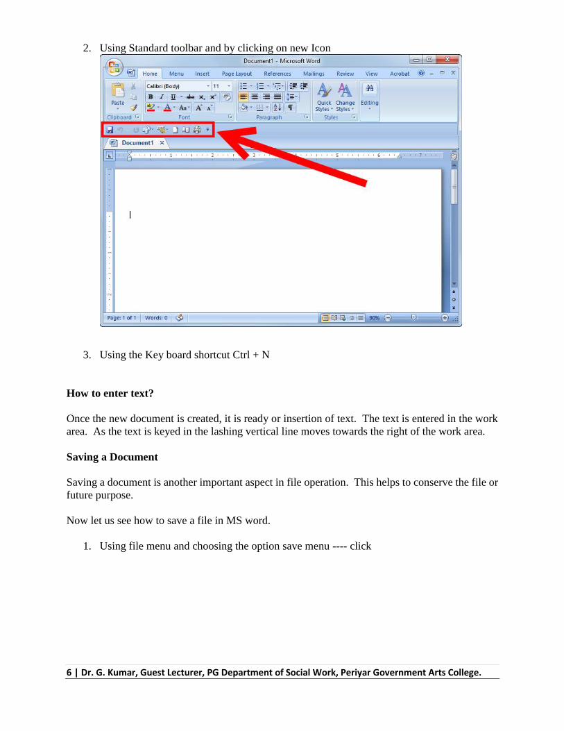
2. Using Standard toolbar and by clicking on new Icon

3. Using the Key board shortcut Ctrl + N

How to enter text?

Once the new document is created, it is ready or insertion of text. The text is entered in the work

area. As the text is keyed in the lashing vertical line moves towards the right of the work area.

Saving a Document

Saving a document is another important aspect in file operation. This helps to conserve the file or

future purpose.

Now let us see how to save a file in MS word.

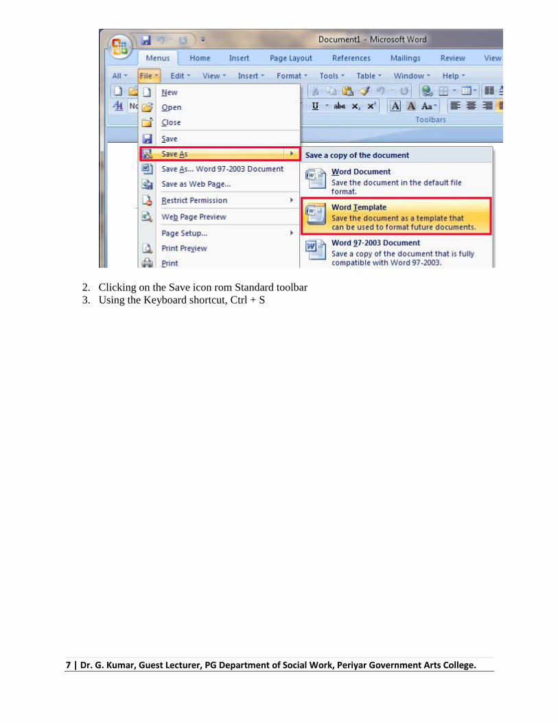
1. Using file menu and choosing the option save menu ---- click


2. Clicking on the Save icon rom Standard toolbar

3. Using the Keyboard shortcut, Ctrl + S


Printing

Go to file

---- click print


Unit – 4

What is Internet?

The internet is a global collection of peoples computers which are linked together by cables

and telephone lines making communication possible among them in a common language.

It is a global collection of inter connected networks.

Network means a facility to share computer equipment, programmes and messages and the

information available at one site.

Internet features:

Internet Takes data from one computer to the other. For such a communication we require

1. The address of the destination

2. A safe way of moving data in the form of electronic signals.

For safe movement of data two set of rules namely Transmission control protocol (TCP)

and Internet protocol (IP) are used in the network software.

For sending a large block of data, to another machine, TCP divides the data into little data

packets.


It also adds special information regarding packet position, error correction code etc. to

make sure that the packets at the destination can be reassembled correctly and without any

damage to data.

The role of IP is to put destination address information on such packets.

On Internet it is not necessary that all the packets will follow the same path from source to

destination.

A special machine called routers tries to load balance various paths that exists on networks.

Another special machine called Gate ways allows different electronic networks to talk to

Internet which uses TCP / IP.

Internet address have two forms:

a. Person understandable expressed as words

b. Machine understandable expressed as numbers

(eg). Jhenryrozario/@ rediffmail.com

The user name is general is the name of the Internet account. This name is the same as the

one, which you may use when logging in to the computer on which you have Internet

account.

Setting up Internet Connection:

1. Dial – up connection:


2. By using a modern and a telephone line, you can connect to a Internet access provider

(VSNL) Satyam, Online, Dishne t etc). Modems can be internal or external

3. On applying for the account you can generally select your user name and password.

4. For using the account you must provide the host machine with username and password.

This process is called as logging in.

5. In dial up account, modem is used to convert computer bits and bytes into modulated

signals that phone lines can transmit.

6. You need communication software like internet explorer, Netscape navigator

Types of Networks:

LAN (Local Area Network) – The computers are geographically else to each other (that is

in the same building).

WAN (Wide Area Network) – The computers are farther apart and are connected by

telephone lines or radio waves. The largest WAN in existence is the Internet.

On LAN can be connected to another LAN over any distance via telephone lines and radio

waves. A System of LANS connected in this way is called WAN.

Uses of LAN:


LANs are used to connect personal computers. So any computer is able to access data

anywhere in the LAN. Thus many uses can share expensive devices such as laser printers or data.

Users can also send e-mail or engage in chat sessions.

TCP / IP

Transmission control protocol / Internet Protocol TCP / IP is nothing but collection of rules

(or protocols) that governs the way data travels form one machine to another access networks.

Internet is bared on TCP / IP.

The IP does the Following:

1. Envelopes and addresses the data

2. Enables the network to read the envelope and forward the data to the destination.

3. Defines how much data can fit into a single envelope. (a packet).

4. The addressed and packaged data is sent over the network to its destination.

The TCP Component does the following:

1. Breaks data up into packets so that the network can handle it efficiently.

2. Verifies whether all the packets arrived at their destination.

3. Reassembles data.


TCP / IP can be compared to transfer from one part of the country to other part.

Hypertext Transfer Protocol (ATTP):

It is a set of rules that governs the transfer of hypertext between two or more computers.

http://WWW.rediffmail.com

The World Wide Web (WWW) encompasses the universe of information that is available

via http. Hypertext is a text that is specially coded using a standard system called Hypertext markup

Language (HTML). The HTML codes are used to create links. There links can be textual or

graphic, and when clicked on can link the user to another resource.

Usually hypertext links will be blue in colour and will be underlined. When you more the

more pointer over a hypertext links the pointer changes its shape to that of a hand, as will be

highlighted.

Domain Name:

A domain name is a way to identify and locate computers connected to the internet. A

domain name always contains two or more components reparated by periods called dots.

(eg). microsoft.com

The last portion of the domain name is the top level domain name and describes the type

of organization holding that name.

http://www.rediffmail.com/


Some of the major Categories are:

.com - commercial entities

.deu - education institutions

.org - miscellaneous organizations that don’t fit any other

category such as not profit groups

.net - organization directly involved in Internet operations.

“.in, uk” - Country codes. “in “ for India and “uk” for United

Kingdom

World Wide Web (WWW):

It is the graphical Internet service that provides a network of interactive documents and the

software to access them.

It is based on documents called pages that combine text, pictures, forms sound, animation

and hypertext links.

To navigate the WWW, users ‘surf’ from one page to another by pointing and clicking on

the hyper links in text or graphics.

WWW is not hierarchical. It is non – linear. that names we can jump from on links to

another. We can go directly to a resource if we know the URL (Uniform Resource Locator)

Use Mail Merge in Microsoft Word

Mail Merge is most often used to print or email form letters to multiple recipients.

Using Mail Merge, you can easily customize form letters for individual recipients.

Mail merge is also used to create envelopes or labels in bulk.

This feature works the same in all modern versions of Microsoft Word: 2010, 2013, and 2016.

1. In a blank Microsoft Word document, click on the Mailings tab, and in

the Start Mail Merge group, click Start Mail Merge.

2. Click Step-by-Step Mail Merge Wizard.

3. Select your document type. In this demo we will select Letters. Click Next:

Starting document.

4. Select the starting document. In this demo we will use the current (blank)

document. Select Use the current document and then click Next: Select

recipients.

o Note that selecting Start from existing document (which we are not

doing in this demo) changes the view and gives you the option to

choose your document. After you choose it, the Mail Merge Wizard

reverts to Use the current document.

5. Select recipients. In this demo we will create a new list, so select Type a new

list and then click Create.

o Create a list by adding data in the New Address List dialog box and

clicking OK.

o Save the list.

o Note that now that a list has been created, the Mail Merge Wizard

reverts to Use an existing list and you have the option to edit the

recipient list.

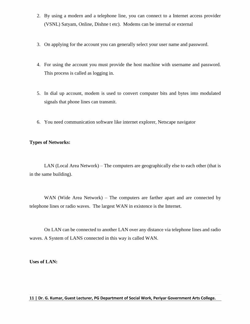
o Selecting Edit recipient list opens up the Mail Merge

Recipients dialog box, where you can edit the list and select or

unselect records. Click OK to accept the list as is.

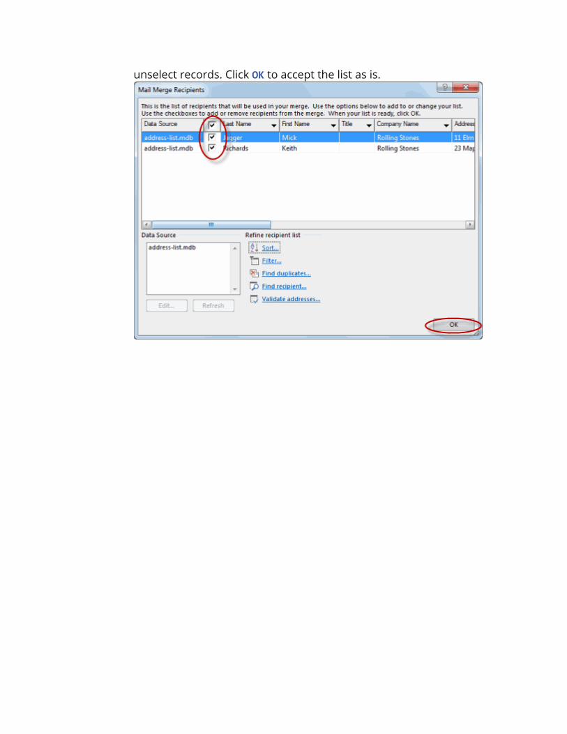
o Click Next: Write your letter.

6. Write the letter and add custom fields.

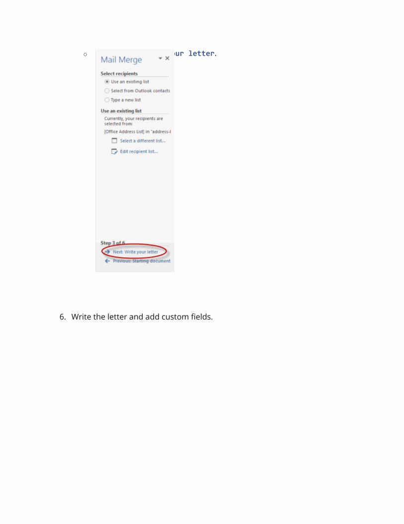
o Click Address block to add the recipients' addresses at the top of the

document.

o In the Insert Address Block dialog box, check or uncheck boxes and

select options on the left until the address appears the way you want it

to.

o Note that you can use Match Fields to correct any problems.

Clicking Match Fields opens up the Match Fields dialog box, in

which you can associate the fields from your list with the fields

required by the wizard.

7. Press Enter on your keyboard and click Greeting line... to enter a

greeting.

8. In the Insert Greeting Line dialog box, choose the greeting line format by

clicking the drop-down arrows and selecting the options of your choice, and

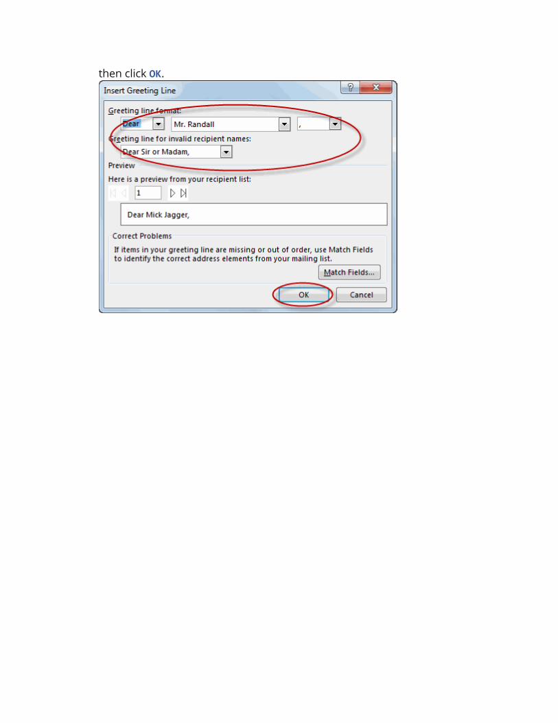
then click OK.

9. Note that the address block and greeting line are surrounded by chevrons («

»). Write a short letter and click Next: Preview your letters.

Preview your letter and click Next: Complete the merge.

Click Print to print your letters or Edit individual letters to further personalize

some or all of the letters.

1

MS - ExcelMicrosoft Excel Basics

Dr. G. Kumar

Guest Lecturer


Periyar Government Arts College, Cuddalore

Excel L

esso

n 1

Pasewark & Pasewark Microsoft Office 2010 Introductory 222

Objectives

Define the terms spreadsheet and worksheet.

Identify the parts of a worksheet.

Start Excel, open an existing workbook, and

save a workbook.

Move the active cell in a worksheet.

Excel L

esso

n 1


Objectives (continued)

Select cells and enter data in a worksheet.

Edit and replace data in cells.

Zoom, preview, and print a worksheet.

Close a workbook and exit Excel.

Excel L

esso

n 1


Vocabulary

active cell

active worksheet

adjacent range

cell

cell reference

column

formula

Formula Bar

landscape orientation

Microsoft Excel 2010

(Excel)

Name Box

nonadjacent range

portrait orientation

Excel L

esso

n 1


Vocabulary (continued)

range

range reference

row

sheet tab

spreadsheet

workbook

worksheet

Excel L

esso

n 1

Pasewark & Pasewark Microsoft Office 2010 Introductory

Introduction to Spreadsheets

Microsoft Excel 2010 is the spreadsheet

program in Microsoft Office 2010.

A spreadsheet is a grid of rows and columns

in which you enter text, numbers, and the

results of calculations.

In Excel, a computerized spreadsheet is

called a worksheet. The file used to store

worksheets is called a workbook.

666

Excel L

esso

n 1


Starting Excel

Start Excel from the Start menu in Windows.

Click the Start button, click All Programs, click

Microsoft Office, and then click Microsoft Excel

2010.

The Excel program window has the same basic

parts as all Office programs: the title bar, the

Quick Access Toolbar, the Ribbon, Backstage

view, and the status bar.

Excel L

esso

n 1


Starting Excel (continued)

Excel program window

8

Excel L

esso

n 1


Exploring the Parts of the Workbook

Each workbook contains three worksheets by

default. The worksheet displayed in the work

area is the active worksheet.

Columns appear vertically and are identified

by letters. Rows appear horizontally and are

identified by numbers.

A cell is the intersection of a row and a

column. Each cell is identified by a unique

cell reference.9

Excel L

esso

n 1


Exploring the Parts of the Workbook (continued)

The cell in the worksheet in which you can type

data is called the active cell.

The Name Box, or cell reference area, displays

the cell reference of the active cell.

The Formula Bar displays a formula when a

worksheet cell contains a calculated value.

A formula is an equation that calculates a new

value from values currently in a worksheet.

10

Excel L

esso

n 1


Opening an Existing Workbook

Opening a workbook means loading an

existing workbook file from a drive into the

program window.

To open an existing workbook, you click the

File tab on the Ribbon to display Backstage

view, and then click Open in the navigation

bar. The Open dialog box appears.

11

Excel L

esso

n 1


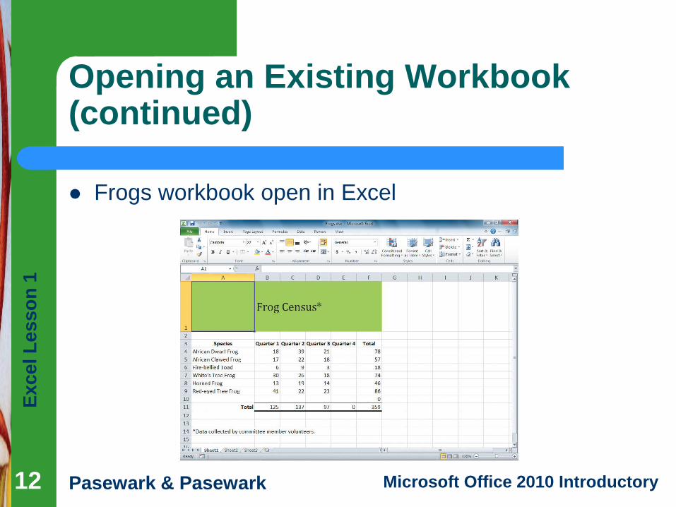
Opening an Existing Workbook (continued)

Frogs workbook open in Excel

12

Excel L

esso

n 1


Saving a Workbook

13

The Save command saves an existing

workbook, using its current name and save

location.

The Save As command lets you save a

workbook with a new name or to a new

location.

Excel L

esso

n 1


Moving the Active Cell in a Worksheet

14

The easiest way to change the active cell in a

worksheet is to move the pointer to the cell

you want to make active and click.

You can display different parts of the

worksheet by using the mouse to drag the

scroll box in the scroll bar to another position.

You can also move the active cell to different

parts of the worksheet using the keyboard or

the Go To command.

Excel L

esso

n 1


Moving the Active Cell in a Worksheet (continued)

Keys for moving the active cell in a worksheet

15

Excel L

esso

n 1


Selecting a Group of Cells

A group of selected cells is called a range.

The range is identified by its range reference,

for example, A3:C5.

In an adjacent range, all cells touch each

other and form a rectangle.

– To select an adjacent range, click the cell in a

corner of the range, drag the pointer to the cell in

the opposite corner of the range, and release the

mouse button.

16

Excel L

esso

n 1


Selecting a Group of Cells (continued)

A nonadjacent range includes two or more

adjacent ranges and selected cells.

– To select a nonadjacent range, select the first

adjacent range or cell, press the Ctrl key as you

select the other cells or ranges you want to

include, and then release the Ctrl key and the

mouse button.

17

Excel L

esso

n 1


Entering Data in a Cell

Worksheet cells can contain text, numbers,

or formulas.

– Text is any combination of letters and numbers

and symbols.

– Numbers are values, dates, or times.

– Formulas are equations that calculate a value.

You enter data in the active cell.

18

Excel L

esso

n 1


Changing Data in a Cell

You can edit, replace, or clear data.

You can edit cell data in the Formula Bar or in the cell. The contents of the active cell always appear in the Formula Bar.

To replace cell data, select the cell, type new data, and press the Enter button on the Formula Bar or the Enter key or the Tab key.

To clear the active cell, you can use the Ribbon, the keyboard, or the mouse.

191919

Excel L

esso

n 1


Searching for Data

The Find command locates data in a

worksheet, which is particularly helpful when

a worksheet contains a large amount of data.

You can use the Find command to locate

words or parts of words.

The Replace command is an extension of the

Find command. Replacing data substitutes

new data for the data that the Find command

locates.20

Excel L

esso

n 1


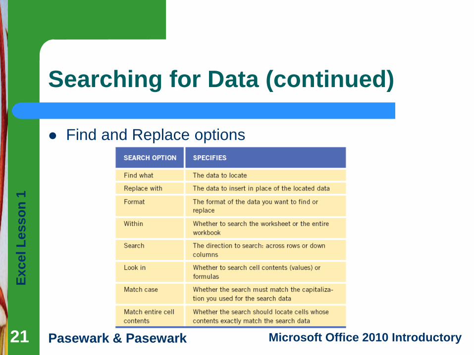
Searching for Data (continued)

Find and Replace options

21

Excel L

esso

n 1


Zooming a Worksheet

You can change the magnification of a

worksheet using the Zoom controls on the

status bar.

The default magnification for a workbook is

100%.

For a closer view of a worksheet, click the

Zoom In button or drag the Zoom slider to

the right to increase the zoom percentage.

22

Excel L

esso

n 1


Zooming a Worksheet (continued)

Zoom dialog box and controls

23

Excel L

esso

n 1


Previewing and Printing a Worksheet

You can print a worksheet by clicking the File

tab on the Ribbon, and then clicking Print in

the navigation bar to display the Print tab.

The Print tab enables you to choose print

settings.

The Print tab also allows you to preview your

pages before printing.

24

Excel L

esso

n 1


Closing a Workbook and Exiting Excel

You can close a workbook by clicking the File

tab on the Ribbon, and then clicking Close in

the navigation bar. Excel remains open.

To exit the workbook, click the Exit command

in the navigation bar.

25

Excel L

esso

n 1


Summary

In this lesson, you learned:

The primary purpose of a spreadsheet is to solve

problems involving numbers. The advantage of using

a computer spreadsheet is that you can complete

complex and repetitious calculations quickly and

accurately.

A worksheet consists of columns and rows that

intersect to form cells. Each cell is identified by a cell

reference, which combines the letter of the column

and the number of the row.

26

Excel L

esso

n 1


Summary (continued)

The first time you save a workbook, the Save As dialog

box opens so you can enter a descriptive name and

select a save location. After that, you can use the Save

command in Backstage view or the Save button on the

Quick Access Toolbar to save the latest version of the

workbook.

You can change the active cell in the worksheet by

clicking the cell with the pointer, pressing keys, or using

the scroll bars. The Go To dialog box lets you quickly

move the active cell anywhere in the worksheet.

27

Excel L

esso

n 1


Summary (continued)

A group of selected cells is called a range. A range is

identified by the cells in the upper-left and lower-right

corners of the range, separated by a colon. To select

an adjacent range, drag the pointer across the

rectangle of cells you want to include. To select a

nonadjacent range, select the first adjacent range,

hold down the Ctrl key, select each additional cell or

range, and then release the Ctrl key.

28

Excel L

esso

n 1


Summary (continued)

Worksheet cells can contain text, numbers, and

formulas. After you enter data or a formula in a cell,

you can change the cell contents by editing,

replacing, or deleting it.

You can search for specific characters in a

worksheet. You can also replace data you have

searched for with specific characters.

29

Excel L

esso

n 1


Summary (continued)

The zoom controls on the status bar enable you to

enlarge or reduce the magnification of the worksheet

in the worksheet window.

Before you print a worksheet, you should check the

page preview to see how the printed pages will look.

When you finish your work session, you should save

your final changes and close the workbook.

30

SPSSStatistical Package for Social Science

UNIT - 3

Introduction

– Software tool

– Comprehensive

– All type of data

Features of SPSS

• It is easy to learn and use

• It is full range of Data management and editing tool

• It provides in-depth statistical analysis

• It offers complete reporting and preventative

Opening SPSS• Start → All Programs → SPSS 20

SPSS Window

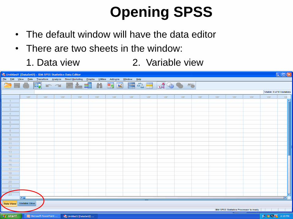
Opening SPSS

• The default window will have the data editor

• There are two sheets in the window:

1. Data view 2. Variable view

Variable View window• This sheet contains information about the data set that is stored

with the dataset

• Name

– The first character of the variable name must be alphabetic

– Variable names must be unique, and have to be less than 64

characters.

– Spaces are NOT allowed.

Variable View window: Type• Type

– Click on the ‘type’ box. The two basic types of variables that you will use

are numeric and string. This column enables you to specify the type of

variable.

Variable View window: Width• Width

– Width allows you to determine the number of characters SPSS will allow to be entered for the variable

Variable View window: Decimals

• Decimals

– Number of decimals

– It has to be less than or equal to 16

3.14159265

Variable View window: LabelLabel

– You can specify the details of the variable

– You can write characters with spaces up to 256 characters

Variable View Window: Values• Values

– This is used and to suggest which numbers represent

which categories when the variable represents a

category

Defining the value labels• Click the cell in the values column as shown below

• For the value, and the label, you can put up to 60 characters.

• After defining the values click add and then click OK.

Click

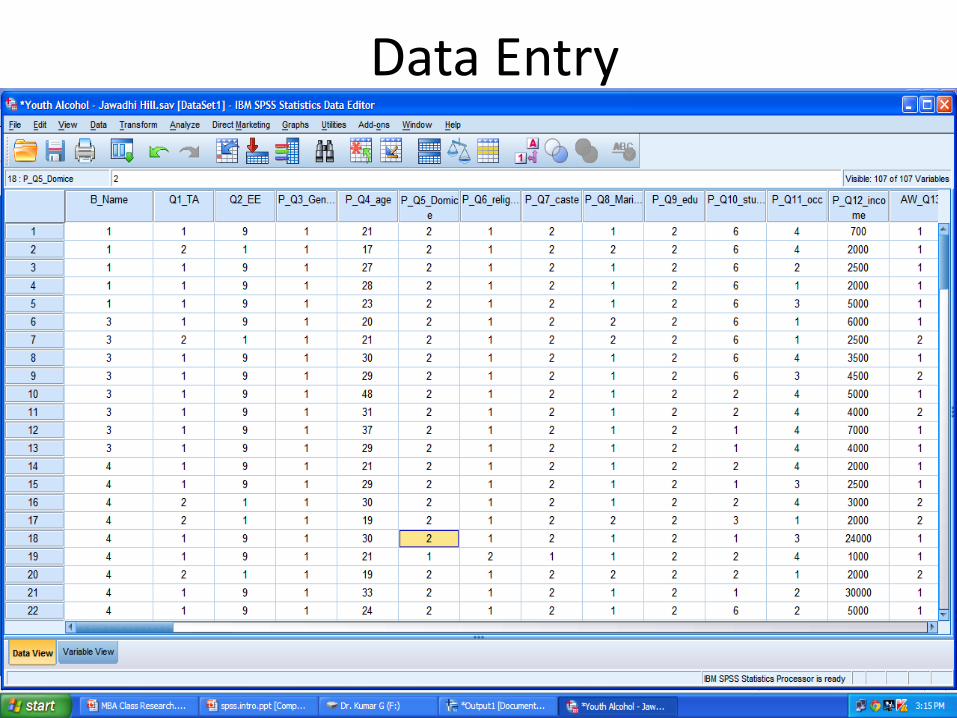
Data Entry

The basic analysis

Table and Statistics

Bar chart

Cross Table & Chi-square test

Recode

Thank You

Unit – IV

Creating data file, syntax file and output file

Unit – IV

Creating data file, syntax file and output file

Assigning names and labels to Variables and Values:

Variable Names: are names used by SPSS to refer to variables e.g Var000001. Since

this is not informative, we need to give meaningful headings to column headings.

Choose any name that makes meaning to you. But they cannot be longer than 8

characters. The name can be used only once. No full stop, no punctuation characters and

no blank in between.

Variable Label: Variable labels explain what the variable is. They can have upto 120

characters and can contain any space or characters. They are added to the output.

Value Labels: are added to the output to explain what a particular value on a variable

denotes.

Indo different variable

1. Click on one of the cells in the column which has to be named.

2. From the menu bar select Data Define Variable.

3. You will get a dialogue box with the curser in the box marked variable name.

4. Type the new name of the variable.

Variable Labels:

To assign variable labels …..

1. Click on the labels button in the define variable dialogue box.

2. You will get another dialogue box with heading Define labels.

3. Type the label into the text box.

Value Labels:

1. Go to Define labels dialogue box

2. Move the curser to the value text box and type the value (e.g) 1,2.

3. Then type the text in the value label text box and click on ‘Add’ button.

4. Use ‘change’ ‘Remove’ button to modify values

Missing Value:

When a respondent fails to provide a response on a variable, it is encoded as ‘missing

value’

1. Go to Define variable dialogue box and click on missing values, button.

2. You will get ‘Define missing values box’

3. Go to Discrete missing value boxes and type the missing value numbers and click

continue.

4. You can give one number no response given, another for don’t know and another

for undecided.

5. Don’t give genuine data value.

Retrieving Data Files:

To retrieve data from floppy disk

1. Insert the floppy in the disk driver.

2. Click the word file.

3. Click on open and you will be presented with open file window.

4. Click on the look in field and select A: drive (any drive you want C: , D:)

5. Next go to files of type click on SPSS (*.rav)

6. Now you will see names of files your disk.

7. Click the name of the file you want. Click.

8. It will appear in the file name.

9. Click open.

10.

Importing or Transferring of Data files:

Data can be entered out side SPSS. It can be entered in EXCEL or MS WORD,

and can be imported to SPSS.

From word Processor:

1. When using MS-WORD, use tab between each variable for simplicity and save it.

2. Go to file, click open.

3. Open ‘Files of type’ drop down menu.

4. Choose Tab- delimited

5. Type the name of the file in the file name box. If it is in a floppy, select A drive,

and the file and click OK.

Transforming data files from others packages:

You can save data in Excel, and for that you do not need a computer with SPSS.

When preparing the data in Excel put variable names in the first row of the sheet. When

imported there will form column names in SPSS file.

1. Select file, click open.

2. Open file dialogue box presented.

3. Go to types of files – select Excel

4. Open driver drop down menu and select appropriate drive.

5. Select the file and click open. It will be inserted in the file name box.

6. Click open, data will be transferred in SPSS.

Saving the Data file: (For the first time)

1. From menu bar, select file – save as

2. You will be presented with save data as dialogue box.

3. Type the file name in the file name box. Choose an appropriate name you will

renumber.

4. Open the drives drop – down list and click on the icon for the drive ‘J’ this means

the your file will be stared in that drive.

5. Open save as type drop down list. It will contain many file formats. Choose

SPSS (*sa).

6. Click OK

7. The name will appear in the Title bar of the data editor window.

Note: It is good idea to restrict file name to 8 characters became some suftares still

reconcile only the first 8 characters.

Saving the Data file for successive times:

1. Select file - Save or save save icon on menu bar or control – s

2. The version you are saving will overwrite the existing one.

3. If you want to keep the old version as well as current one, use file/ save as and

type a different name for the current one.

Printing the data file:

1. Check the window to be printed.

2. Go to file – print

3. Print dialogue box will appear with the name of the file to be printed, in the title

bar.

4. Type the number required in the copies box.

5. Choose print quality in the properties box.

6. click on OK.

Note:

1. If you do not want grid lines, select view grid lines and use the option

suppressing grid lines.

2. Similarly if you want to have value lavesh instced of values to be printed, then

GU View / value labels. / or use Icon (Pencial).

Adding cases: (inserting new case)

1. Select any cell in the case row below the parction in which you want to insert the

new case

2. From the menus choose. Data

3. Choose Insert cases

4. A new row is inserted for the case and all variables receive the system missing

value.

Inserting new Variables:

1. Select any cell in the variables (column) to the right position where you want to

insert the new variable.

2. From the menus choose data

3. Choose insert variable.

4. A new variable is inserted with the system missing value for all cases.

Using menus to analysis data:

1. Click the analyse drop down menu in the application window.

2. Each entry (Reparts. Description statistics, non parametere has on arrowhead to

show that there is another menu which can be obtained by elicking on the entry)

(e.g) If you click on Descriptive statistics, you will get sub menu such as

- Frequencies ….

- Descriptives

- Explore

- Cross tables.

3. If you click frequencies ….. you will get a dialogue box.

If you want to calculate the frequencies:

For example you want to calculate how much percentage of your respondents are

illiterates, and literate.

1. Go to statistics, - Descriptive statistics – Frequencies

2. You will get frequency dialogue box. If will contain list of variables on left side

box and an empty box listed variables on the sight side. There will be an arrow in

between.

3. Click the variable ‘educational status’, and click the arrow. That variable will

appear in variable box.

4. If you want to simultaneously do frequencies for many variables choose them all

in the variable box.

5. click OK button.

6. Once SPSS has completed the analysis, the result will appear in the output

navigator window.

7. If you click ‘Reset’, variable you have selected for analysis will be returned to the

list of variables box on the self.

8. If you click ‘cancel’, no analysis will be done, and you will return to analysis

menu bar.

9. If you click help, you will access to SPSS Help facility.

Output Navigator window:

1. The output navigator window is divided into two panes.

2. Pane on the left shows contnts of SPSS output in outline form

SPSS output

Descriptives

Title

Notes

3. The pane on the right provides results of statistical analysis.

4. By clicking on any item on the outline on the left the corresponding details

appears on the right. This in called navigation. Useful when the output in empty.

5. Click xxxxxx will appear. You can edit title by double clicking on that and make

the changes.

6. Use Navigation facility to choose other statistical analysis, without sewlling thom

entire output researching for the portion you want.

7. Valid column indicater valid cases without missing

8. In the missing indicaters missing value for each cell data final column consist of

what variables are analysied next column consxxxx number.

Saving the Output:

1. File pull down manue select save as

2. Enter the name of the file into file name box. Drive, Folder)

3. If you want to switch between data editor window and the output window, use the

button at the xxxxxxxx task bar at the button.

4. If you want to save your output in the same file, open that file after opening the

data editor window. Keep it active. Switech over to data editor window. Do

analysis and end it will be saved in that file.

(Danger of replacing which saving)

Printing Output file:

1. Load the output file into a word processor.

Creating Charts: Bar charts:

1. Go to graph menu and select ‘Bar’ the bar charts dialog box will open.

2. This will have three options : simple, dustered stacked. If you have only one

variable i.o gender, choose simple. If you have more than one variable, gender

and percentage of pass in exams choose dustered or stacked.

3. Choose simple – Click De fine.

4. In the simple Bar dialogue box, choose the variable to be graphed, click it. Then

click arrow near the category axis box, (x axis).

5. Go to ‘ Bars represent’ Box at the top. You have different options like N of cases

(frequencies) and percentage of cases etc.

6. Click % cases

7. Use option button in the lower right hand cover of you want to tread missing

values there will be a box with name Display groups defined by missing values.

Deselect it, by clicking on the check mark. Click continues

8. Go to Titles button located in the lowers right hand corner. Open the dialogue

box.

9. specify the titles and titles and figure number under foot notes.

10. Click OK. You will get bar chart.

Editing Bar Chart:

1. To edit double click on the chart. You will get Windows chart Editor.

2. Go to chart. Go to axis you will get

3. Axis selection. Choose scale and click OK.

4. Modify axis title if you want. Use title justification In the box titled range, put

minimum as 0 and maximum as 100 (If you want the picture of represent for

100%)

5. In the major division and mixor divisions dialogue box, put increments of 10

usually.

6. Use Bar spacing (Bar margin - % of inner frame Inter bar spacing - % of bar

width.

7. Instead of using title use foot note. Type figure 1, under food note 1 and the title

in foot note 2. justify it to center click OK.

8. You need to choose legend if you are depicting more than one variable. Select

legnd and select display legend. If you don’t want derelect it.

9. You can modify title and Justify it. If you want to add to labels select the word in

tables. If will appear in selected label. Type the word you want to insert click

champed, and then OK.

10. Select outer frame and inner frame as you xxxxxx.

Recoding Variables:

1. Under transform menu, choose recode

2. You will get a box with Indo same variable

Indo different variable

Choose Indo different variable

You will get recode into pfifferent variable dialogue

bad

3. select the variable to be recoded (Income) and place it in the Input variable –

output variable box.

4. Go to output variable box. given a new name the new Income define the label

clearly (monthly Income of the respondents). Click change. New name will be

added to the emitting name of the variable.

5. Choose old and new values button. You will get the dialogue box. In the left

hand side you have old value box on the right side new value box / go to old value

box.

6. Several option are available. Select range through for converting actual income

into coder select value if you want to give new values to existing old values (e.g)

attitude sealer.

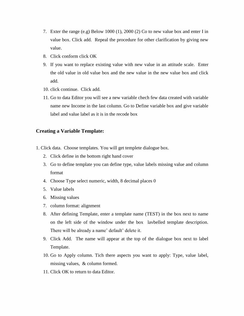
7. Exter the range (e.g) Below 1000 (1), 2000 (2) Co to new value box and enter I in

value box. Click add. Repeal the procedure for other clarification by giving new

value.

8. Click conform click OK

9. If you want to replace existing value with new value in an attitude scale. Enter

the old value in old value box and the new value in the new value box and click

add.

10. click continue. Click add.

11. Go to data Editor you will see a new variable chech few data created with variable

name new Income in the last column. Go to Define variable box and give variable

label and value label as it is in the recode box

Creating a Variable Template:

1. Click data. Choose templates. You will get templete dialogue box.

2. Click define in the bottom right hand cover

3. Go to define template you can define type, value labels missing value and column

format

4. Choose Type select numeric, width, 8 decimal places 0

5. Value labels

6. Missing values

7. column format: alignment

8. After defining Template, enter a template name (TEST) in the box next to name

on the left side of the window under the box lavbelled template description.

There will be already a name’ default’ delete it.

9. Click Add. The name will appear at the top of the dialogue box next to label

Template.

10. Go to Apply column. Tich there aspects you want to apply: Type, value label,

missing values, & column formed.

11. Click OK to return to data Editor.

Applying a variable Template:

1. To apply a template to other variables, you need not have defined their variable

name you can also it later.

2. Highlight the column you want to apply the templete. If you have already given

variable names just highlights the names of the variables in the data editor.

3. From the menu choose data and than templates.

4. Your Template ’Test’ will appear. If it does not appear, select it byclicking the

down arrow

5. Click OK template will be applied to the selected columns

6. If you have not defined, variable name and variable label, do it now.

Cross Tabulation of Variables:

1. Click analysis – Descriptive statistics

2. Go to cross tabs.

3. Highlight the variable and place it in row box.

4. Highlight another variable and place it column box.

5. Click cells under percentages there will be three options. Row total, column total

and total number of cases.

6. Choose either column total are both now end column total select continue.

7. click OK.

8. Interpretation need to focus a both row and column percentages and row and

column totals.

Application of Chi square test:

1. Chi square is a test of significance that is most appropriate for nominal items.

2. It estimates the probability that the association between variables is a result of

randon chance or sampling error by comparing the actual or observed distribution

of responses with the distribution of responses we would expect if there were

absolutely no association between two variables.

Calculation chi square test:

1. Click analyze – Descriptive statistics

2. Go to cross tabs.

3. Highlight dependent variable and transfer to rows.

4. Highlight independent variable and transfer to columns.

5. Click cells. Select column percentage or both column and row percentage. Click

continue.

6. Click statistics click chi square. Click continue.

7. click OK

Reading Output:

The first row gives chi square value, degree of freedom and the probability value

(the probability is far less than .001, if that is the p value)

Calculation of central tendency and dispersion:

For continuous variables(e.g) age, income

1. Analyze – Descriptive statistics

2. Choose Descriptives

3. Select mean. Standard deviation, minimum and maximum.

4. Click continue.

5. click OK.

Std. Deviation tells us how far we need to go above and below the means to include

roughly tow thirds of all the easssss

To obtain Pie Chart:

1. Graph

2. Pie – pie charts dialogue box.

3. Data in chart : summaries for group of data

4. Click define.

5. Select the variable you want to define the categories or slices.

6. Go to title Go to foot note. Title 1, Title 2,

7. Click OK

8. Double click

9. Chart option : Pie option: Position, collapx slices less than 5%,

10. under labels : Text percent will be already selected not select it.

11. Go to Edit text.

12. Go to label formal position

13. Title fortune outline farm

Discrete / Categorical variable

(e.g) Gender (how many men / woman are there) choose

1. Analysis – Descriptive statistics

2. Frequencies.

3. Variables name on the box

4. Click statistics choose option.(mode etc)

5. Click continue. Click OK.

Mode (the most frequent response)

Creating a Syntax File :

A syntax file is a file that contains the commands for the analyses we have

requested expressed in SPSS’s language.

Uses of Syntax File :

1. It gives a record of the analyses performed.

2. It helps to do the analysis directly by running the commands from systax

window. We need not go through the process of selection menu a second time.

3. By saving syntax window as a separate file we have a permanent copy to use it

again.

Creating Syntax File :

1. Select items from the menu for performing a statistical test.

2. Click paste. This will paste the SPSS language command for the statistical

procedure you have selected into a separate syntax window.

3. Subsequent uses of ‘Paste’ will add the current commands to the syntax window

adding them to the existing contents.

4. The Syntax window can be saved as a file and edited.

5. All commands must start on a new line and must end in a full stop.

6. Sub commands are used to specify how the procedure should operate. Sub

Commands are usually separated by / character.

Running Commands from a Syntax Window:

1. Select the commands to be used procedure.

2. Click on the Run button.

3. If you want to run all the commands use Edit / Select All option. To run only one

command put the cursor anywhere in the line containing the command and click

on Run.

Saving the Syntax Window as a Syntax File :

1. File Save As

Retrieving a Saved Syntax File :

1. File Open SPSS Syntax.

Opening Another Syntax Window :

1. File New SPSS Syntax.

Transferring Syntax files to a Word Processar :

List

UNIT – 5

ANALYSIS OF DATA

Data

To begin the process of adding data, just click on the first cell that is located in the upper

left corner of the datasheet. It's just like a spreadsheet. You can enter your data as shown.

Enter each datapoint then hit [Enter]. Once you're done with one column of data you can

click on the first cell of the next column.

These data are taken from table2.1 in Howell's text. The first column represents

"Reaction Time in 100ths of a second" and the second column indicates "Frequency".

If you're entering data for the first time, like the above example, the variable names will

be automatically generated (e.g., var00001, var00002,....). They are not very informative.

To change these names, click on the variable name button. For example, double click on

the "var00001" button. Once you have done that, a dialog box will appear. The simplest

option is to change the name to something meaningful. For instance, replace "var00001"

in the textbox with "RT" (see figure below).

In addition to changing the variable name one can make changes specific to [Type],

[Labels], [Missing Values], and [Column Format].

[Type] One can specify whether the data are in numeric or string format, in

addition to a few more formats. The default is numeric format.

[Labels] Using the labels option can enhance the readability of the output. A

variable name is limited to a length of 8 characters, however, by using a variable

label the length can be as much as 256 characters. This provides the ability to

have very descriptive labels that will appear at the output.

Often, there is a need to code categorical variables in numeric format. For

example, male and female can be coded as 1 and 2, respectively. To reduce

confusion, it is recommended that one uses value labels . For the example of

gender coding, Value:1 would have a correspoding Value label: male. Similarly,

Value:2 would be coded with Value Label: female. (click on the [Labels] button

to verify the above)

[Missing Values] See the accompanying help. This option provides a means to

code for various types of missing values.

[Column Format] The column format dialog provides control over several

features of each column (e.g., width of column).

The next image reflects the variable name change.

Once data has been entered or modified, it is adviseable to save. In fact, save as often as

possible [File => SaveAs].

SPSS offers a large number of possible formats, including their own. A list of the

available formats can be viewed and selected by clicking on the Save as type: , on the

SaveAs dialog box. If your intention is to only work in SPSS, then there may be some

benefit to saving in the SPSS(*.sav) format. I assume that this format allows for faster

reading and writing of the data file. However, if your data will be analyzed and looked by

other packages (e.g., a spreadsheet), it would be adviseable to save in a more universal

format (e.g., Excel(*.xls), 1-2-3 Rel 3.0 (*.wk3).

Once the type of file has been selected, enter a filename, minus the extension (e.g., sav,

xls). You should also save the file in a meaningful directory, on your harddrive or floppy.

That is, for any given project a separate directory should be created. You don't want your

data to get mixed-up.

The process of reading already saved data can be painless if the saved format is in the

SPSS or a spreadsheet format. All one has to do is,

o click on [File => New => Data]

o click on [File => Open] : a dialog box will appear

o navigate to desired directory using the Look in: menu at the top of the

dialog box

o select file type in the Files of type menu

o click on the filename that is needed.

The process of reading existing files is slightly more involved if the format is

ASCII/plain text (see the earlier description of [Freefield] and [Fixed Columns]). As an

example, the ASCII data from table2.1 in the Howell text will be used. A file containing

the data should be included in the accompanying disk for the text. [Note: It was not

present in my disk, so I downloaded the file from Howell's webpage.] I've placed the files

on my harddrive at c:\ascdat. In the case of this set of data,there are four columns

representing observation number, reaction time, setsize, and the presence or absence of

the target stimulus. This information can be found in the readme.txt file that is also on

the disk. Typically, we are aware of the contents of our own data files, however, it doesn't

hurt to keep a record of the contents of such files.

To make life easier the [File => Read ASCII Data => Freefield] will be used.

The resulting dialog box requires that a File , a Name and a Data Type be specified for

each variable, or column of data. The desired file is accessed by clicking on the [Browse]

button, and then navigating to the desired location. Since the extension for the sought

after file is dat there is no need to change the Files of type: selection. However, if the

extension is something else (e.g., *.txt) then it would be necessary to select All files(*.*)

from the Files of type: menu. Since there are 4 variables in this data set, 4 names with the

corresponding type information must be specified. To Add the first variable,

observations, to the list,

o type "obs" in the Name box

o the Data Type is set to Numeric by default. If "obs" was a string variable,

then one would have to click on String

o click on the Add button to include this variable to the list.

o repeat the above procedure with new names and data types for each of the

remaining variables. It is important that all variables be added to the list.

Otherwise, the data will be scrambled.

(Please explore the various options by clicking on any accessible menu item.)

The resulting data files appears in the data editor like the following.

The next section will cover some descriptive statistics.

Descriptive Statistics

We can replicate the frequency analyses that are described in chapter 2 of the text, by

using the file that was just read into the data editor - tab2-1.dat. These analyses were

conducted on the reaction time data. Recall, that we have labelled this data as RT.

To begin, click on [Statistics=>Summarize=>Frequencies]....

The result is a new dialog box that allows the user to select the variables of interest. Also,

note the other clickable buttons along the border of the dialog box. The buttons labelled

[Statistics...] and [Charts...] are of particular importance. Since we're interested in the

reaction time data, click on rt followed by a mouse click on the arrow pointing right. The

consequence of this action is a transference of the rt variable to the Variables list. At this

point, clicking on the [OK] button would spawn an output window with the Frequency

information for each of the reaction times. However, more information can be gathered

by exploring the options offered by the [Statistics...] and [Charts...].

[Statistics...] offers a number of summary statistics. Any statistic that is selected will be

summarized in the output window.

As for the options under [Charts...] click on Bar Charts to replicate the graph in the

text.

Once the options have been selected, click on [OK] to run the procedure. The results are

then displayed in an output window. In this particular instance the window will include

summary statistics for the variable RT, the frequency distribution, and the frequency

distribution. You can see all of this by scrolling down the window. The results should

also be identical to those in the text.

You may have gathered from the above that calculating summary statistics requires

nothing more than selecting variables, and then selecting the desired statistics. The

frequency example allowed us to generate frequency information plus measures of

central tendencies and dispersion. These statistics can be had by clicking directly on

[Statistics=>Summarize=>Descriptives]. Not surprisingly, another dialog box is

attached to this procedure. To control the type of statistics produced, click on the

[Options...] button. Once again, the options include the typical measures of central

tendency and dispersion.

Each time as statistical procedure is run, like [Frequencies...] and [Descriptives...] the

results are posted to an Output Window. If several procedures are run during one session

the results will be appended to the same window. However, greater organization can be

reached by opening new Output windows before running each procedure -

[File=>New=>Output]. Further, the contents of each of these windows can be saved for

later review, or in the case of charts saved to be later included in formattted documents.

[Explore by left mouse clicking on any of the output objects (e.g., a frequency table, a

chart, ...) followed by a right button click. The left left button click will highlight the

desired object, while the right button click will popup a new menu. The next step is to

click on the copy option. This action will store the object on the clipboard so that it can

be pasted to Word for Windows document, for example.....]

Chi-Square & T-Test

The computation of the Chi-Square statistic can be accomplished by clicking on

[Statistics => Summarize => Crosstabs...]. This particular procedure will be your first

introduction to coding of data, in the data editor. To this point data have been entered in a

column format. That is, one variable per column. However, that method is not sufficient

in a number of situations, including the calculation of Chi-Square, Independent T-tests,

and any Factorial ANOVA design with between subjects factors. I'm sure there are many

other cases, but they will not be covered in this tutorial. Essentially, the data have to be

entered in a specific format that makes the analysis possible. The format typcially

reflects the design of the study, as will be demonstrated in the examples.

In your text, the following data appear in section 6.????. Please read the text for a

description of the study. Essentially, the table - below - includes the observed data and

the expected data in parentheses.

Fault Guilty Not Guilty Total

Low 153(127.559) 24(49.441) 177

High 105(130.441) 76(50.559) 181

Total 258 100 358

In the hopes of minimizing the load time for remaining pages, I will make use of the

built in table facilty of HTML to simulate the Data Editor in SPSS. This will reduce the

number of images/screen captures to be loaded.

For the Chi-Square statistic, the table of data can be coded by indexing the column and

row of the observations. For example, the count for being guilty with Low fault is 153.

This specific cell can be indexed as coming from row=1 and column=1. Similarly, Not

Guilty with High fault is coded as row=2 and column=2. For each observation, four in

this instance, there is unique code for location on the table. These can be entered as

follows,

Row Column Count

1 1 153

1 2 24

2 1 105

2 2 76

So, 2 rows * 2 columns equals 4 observations. That should be clear.

For each of the rows, there are 2 corresponding columns, that is reflected in the

Count column. The Count column represents the number of time each unique

combination Row and Column occurs.

The above presents the data in an unambigous manner. Once entered, the analysis is a

matter of selecting the desired menu items, and perhaps selecting additional options for

that statistic. [Don't forget to use the labelling facilities, as mentioned earlier, to

meaningfully identify the columns/variables. The labels that are chosen will appear in

the output window.]

To perform the analysis,

The first step is to inform SPSS that the COUNT variable represents the

frequency for each unique coding of ROW and COLUMN, by invoking the

WEIGHT command. To do this, click on [Data => Weight Cases]. In the

resultant dialog box, enable the Weight cases by option, then move the COUNT

variable into the Frequency Variable box. If this step is forgotten, the count for

each cell will be 1 for the table.

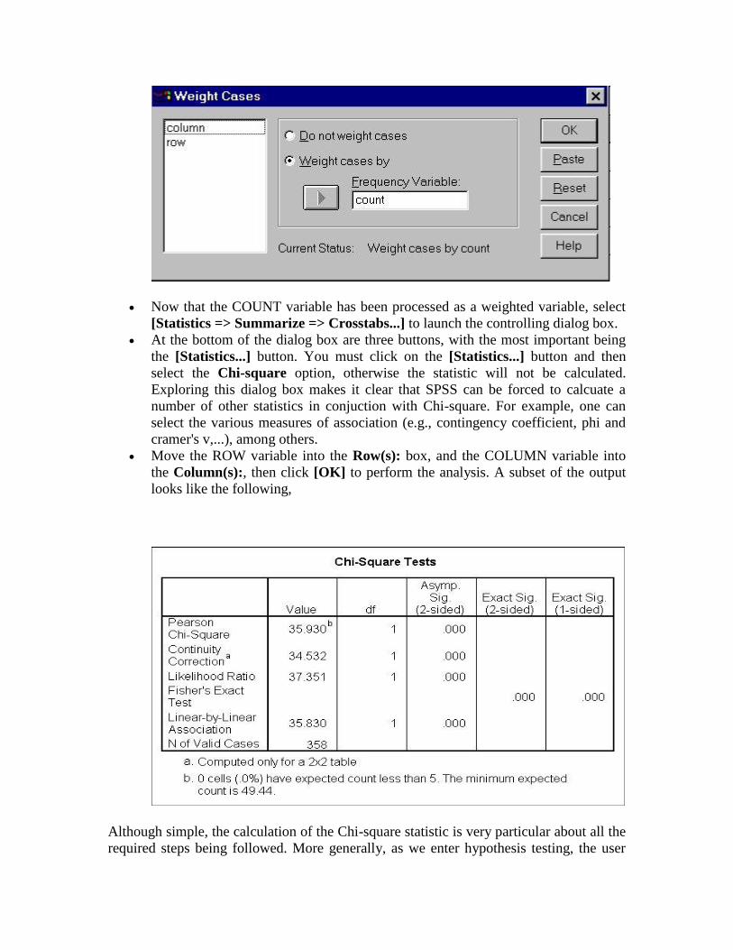
Now that the COUNT variable has been processed as a weighted variable, select

[Statistics => Summarize => Crosstabs...] to launch the controlling dialog box.

At the bottom of the dialog box are three buttons, with the most important being

the [Statistics...] button. You must click on the [Statistics...] button and then

select the Chi-square option, otherwise the statistic will not be calculated.

Exploring this dialog box makes it clear that SPSS can be forced to calcuate a

number of other statistics in conjuction with Chi-square. For example, one can

select the various measures of association (e.g., contingency coefficient, phi and

cramer's v,...), among others.

Move the ROW variable into the Row(s): box, and the COLUMN variable into

the Column(s):, then click [OK] to perform the analysis. A subset of the output

looks like the following,

Although simple, the calculation of the Chi-square statistic is very particular about all the

required steps being followed. More generally, as we enter hypothesis testing, the user

should be very careful and should make use of manuals for the programme and textbooks

for statistics.

T-tests

By now, you should know that there are two forms of the t-test, one for dependent

variables and one for independent variables, or observations. To inform SPSS, or any

stats package for that matter, of the type of design it is necessary to have to different

ways of laying out the data. For the dependent design, the two variables in question must

be entered in two columns. For independent t-tests, the observations for the two groups

must be uniquely coded with a Gruop variable. Like the calculation of the Chi-square

statistic, these calculations will reinforce the practice of thinking about, and laying out

the data in the correct format.

Dependent T-Test

To calculate this statistic, one must select [Statistics => Compare Means => Paired-

Samples T Test...] after enterin the data. For this analysis, we'll use the data from Table

7.3, in Howell.

Enter the data into a new datafile. Your data should look a bit like the following.

That is, the two variables should occupy separate columns...

Mnths_6 Mnths_24

124 114

94 88

115 102

110 2

116 2

139 2

116 2

110 2

129 2

120 2

105 2

88 2

120 2

120 2

116 2

105 2

... ...

... ...

123 132

Note that the variable names start with a letter and are less than 8 characters long.

This is a bit constraining, however, one can use the variable label option to label

the variable with a longer name. This more descriptive name will then be

reproduced in the output window.

To calculate the t statistic click on [Statistics => Compare Means => Paired-

Samples T Test...], then select the two variables of interest. To select the two

variables, hold the [Shift] key down while using the mouse for selection. You will

note that the selection box requires that variables be selected two at a time. Once

the two variables have been selected, move them to the Paired Variables: list.

This procedure can be repeated for each pair of variables to be analyzed. In this

case, select MNTHS_6 and MNTHS_24 together, then move them to the Paired

Variables list. Finally, click the [OK] button.

The critical result for the current analysis will appear in the output window as

follows,

As you can see an exact t-value is provided along with an exact p-value, and this

p-value is greater that the expected value of 0.025, for a two-tailed assessment.

Closer examination indicates several other statistics are presented in output

window.

Quite simply, such calculations require very little effort!

Independent T-tests

When calculating an independent t-test, the only difference involves the way the data are

formatted in the datasheet. The datasheet must include both the raw data and group

coding, for each variable. For this example, the data from table 7.5 will be used. As an

added bonus, the number of observations are unequal for this example.

Take a look at the following table to get a feel for how to code the data.

Group Exp_Con

1 96

1 127

1 127

1 119

1 109

1 143

1 ...

1 ...

1 106

1 109

2 114

2 88

2 104

2 104

2 91

2 96

2 ...

2 ...

2 114

2 132

From the above you can see that we used the "Group" variable to code for the two

variables. The value of 1 was used to code for "LBW-Experimental", while a value of 2

was used to code for "LBW-Control". If you're confused please study the table, above.

To generate the t-statistic,

Clik on [Statistics => Compare Means => Independent-Samples T Test] to

launch the appropriate dialog box.

Select "exp_con" - the dependent variable list - and move it to the Test

Variable(s): box.

Select "group" - the grouping variable list - and move it to the Grouping

Variable: box.

The final step requires that the groups be defined. That is, one must specify that

Group1 - the experimental group in this case - is coded as 1, and Group2 - the

control group in this case - is coded as 2. To do this, click on the [Define

Groups...] button. Click on the [Continue] button to return to the controlling

dialog box.

Run the analysis by clicking on the [OK] button.

The output for the current analysis extracted from the output window looks like

the following.

The p-value of .004 is way lower than the cutoff of 0.025, and that suggests that the

means are significantly different. Further, a Levene's Test is performed to ensure that the

correct results are used. In this case the variances are equal, however, the calculations for

unequal variances are also presented, among some other statistics - some not presented.

In the next section we will briefly demonstrate the calculation of correlations and

regression, as discussed in Chapter 9 of Howell. In truth, you should be able to work

through many statistics with your current knowledge base and the help files, including

correlations and regressions. Most statistics can be calculated with a few clicks of the

mouse.

Correlations and Regression

This will be a brief tutorial, since there is very little that is required to calculate

correlations and linear regressions. To calculate a simple correlation matrix, one must use

[Statistics => Correlate => Bivariate...], and [Statistics => Regression => Linear] for

the calculation of a linear regression.

For this section, the analyses presented in the computer section of the Correlation and

Regression chapter will be replicated. To begin, enter the data as follows,

IQ GPA

102 2.75

108 4.00

109 2.25

118 3.00

79 1.67

88 2.25

... ...

... ...

85 2.50

Simple Correlation

Click on [Statistics => Correlate => Bivariate...], then select and move "IQ" and

"GPA" to the Variables: list. [Explore the options presented on this controlling

dialog box.]

Click on [OK] to generate the requested statistics.

The results from output window should look like the following,

As you can see, r=0.702, and p=.000. The results suggest that the correlation is

significant.

Note: In the above example we only created a correlation matrix based on two variables.

The process of generating a matrix based on more than two variables is not different.

That is, if the dataset consisted of 10 variables, they could have all been placed in the

Variables: list. The resulting matrix would include all the possible pairwise correlations.

Correlation and Regression

Linear regression....it is possible to output the regression coefficients necessary to predict

one variable from the other - that minimize error. To do so, one must select the [Statistics

=> Regression => Linear...] option. Further, there is a need to know which variable will

be used as the dependent variable and which will be used as the independent variable(s).

In our current example, GPA will be the dependent variable, and IQ will act as the

independent variable. Specifically,

Initiate the procedure by clicking on [Statistics => Regression => Linear...]

Select and move GPA into the Dependent: variable box

Select andmove IQ into the Independent(s): variable box

Click on the [OK] to generate the statistics.

Note: A variety of options can be accessed via the buttons on the bottom half of

this controlling dialog box (e.g., Statistics, Plots,...). Many more statistics can be

generated by explore the additional options via the Statistics button.

Some of the results of this analysis are presented below,

The correlation is still 0.702, and the p value is still 0.000. The additional statistics are

"Constant", or a from the text, and "Slope", or B from the text. If you recall, the

dependent variable is GPA, in this case. As such, one can predict GPA with the

following,

GPA = -1.777 + 0.0448*IQ

The next section will discuss the calculation of the ANOVA.

computer application in social work

Documents