computer and internet use in the united states: 2013 · access to broadband technologies, ......

American Community Survey Reports

Computer and Internet Use in the United States: 2013

By Thom File and Camille RyanIssued November 2014ACS-28

U.S. Department of Commerce Economics and Statistics Administration U.S. CENSUS BUREAU

census.gov

INTRODUCTION

For many Americans, access to computers and high-speed Internet connections has never been more important. We use computers and the Internet to complete schoolwork, locate jobs, watch movies, access healthcare information, and find relationships, to name but a few of the ways that we have grown to rely on digital technologies.1 Just as our Internet activities have increased, so too have the num-ber of ways that we go online. Although many American households still have desktop computers with wired Internet connections, many others also have laptops, smartphones, tablets, and other devices that connect people to the Internet via wireless modems and fixed wireless Internet networks, often with mobile broadband data plans.

As part of the 2008 Broadband Data Improvement Act, the U.S. Census Bureau began asking about computer and Internet use in the 2013 American Community Survey (ACS).2 Federal agencies use these statistics to measure and monitor the nationwide development of broadband networks and to allocate resources intended to increase access to broadband technologies, particularly among groups with traditionally low levels of access. State and local governments can use these statistics for similar purposes. Understanding how people in specific cities and towns use computers and the Internet will help businesses and nonprofits better serve their communities as well.

The Census Bureau has asked questions in the Current Population Survey (CPS) about computer use since 1984

1 For more information, see <www.ntia.doc.gov/report/2013 /exploring-digital-nation-americas-emerging-online-experience> and <www.census.gov/hhes/computer/files/2012/Computer_Use _Infographic_FINAL.pdf>.

2 For more background on the ACS, please visit <www.census.gov /acs/www/>.

and Internet access since 1997. While these estimates remain useful, particularly because of the historical con-text they provide, the inclusion of computer and Internet questions in the ACS provides estimates at more detailed levels of geography. The CPS is based on a sample of approximately 60,000 eligible households and estimates are generally representative only down to the state level.3 Computer and Internet data from the ACS, based on a sample of approximately 3.5 million addresses, are available for all geographies with populations larger than 65,000 people and will eventually become available for most geographic locations across the country.4

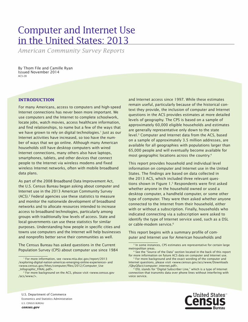
This report provides household and individual level information on computer and Internet use in the United States. The findings are based on data collected in the 2013 ACS, which included three relevant ques-tions shown in Figure 1.5 Respondents were first asked whether anyone in the household owned or used a desktop computer, a handheld computer, or some other type of computer. They were then asked whether anyone connected to the Internet from their household, either with or without a subscription. Finally, households who indicated connecting via a subscription were asked to identify the type of Internet service used, such as a DSL or cable-modem service.6

This report begins with a summary profile of com-puter and Internet use for American households and

3 In some instances, CPS estimates are representative for certain large metropolitan areas.

4 See the “Source of the Data” section located in the back of this report for more information on future ACS data on computer and Internet use.

5 For more background and the exact wording of the computer and Internet questions, please visit <www.census.gov/acs/www/Downloads /QbyQfact/computer_internet.pdf>.

6 DSL stands for “Digital Subscriber Line,” which is a type of Internet connection that transmits data over phone lines without interfering with voice service.

2 U.S. Census Bureau

individuals, followed by a section addressing the types of Internet connections households use.7, 8 The final sec-tion presents more detailed geographic results for both states and metropolitan areas.

7 In this report, the term “computer ownership” will be used for the sake of brevity, although the data refer to households whose members own or use a computer.

8 When “Internet use” is discussed, the reported percentage refers to households with a subscription to an Internet service plan. About 4.2 percent of households reported home Internet use without a sub-scription, and in this report, these households are not included in the Internet use estimates.

HIGHLIGHTS

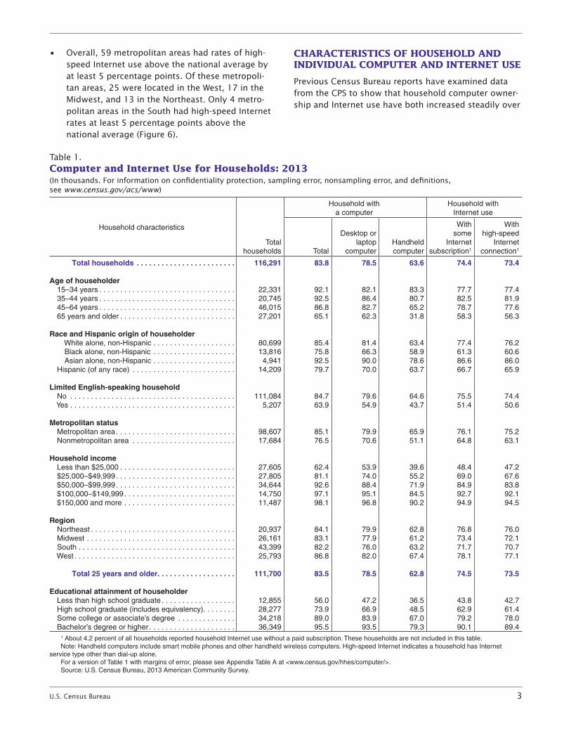
• In 2013, 83.8 percent of U.S. households reported computer ownership, with 78.5 percent of all households having a desktop or laptop computer, and 63.6 percent having a handheld computer (Table 1).

• In 2013, 74.4 percent of all households reported Internet use, with 73.4 percent reporting a high-speed connection (Table 1).

• Household computer ownership and Internet use were most common in homes with relatively young householders, in households with Asian or White householders, in households with high incomes, in metropolitan areas, and in homes where householders reported relatively high levels of educa-tional attainment (Table 1).9

• Patterns for individuals were similar to those observed for households with computer owner-ship and Internet use tending to be highest among the young, Whites or Asians, the affluent, and the highly educated (Table 2).

• The most common household connection type was via a cable modem (42.8 percent), followed by mobile broadband (33.1 percent), and DSL con-nections (21.2 percent). About one-quarter of all households had no paid Internet subscription (25.6 percent), while only 1.0 percent of all households reported connecting to the Internet using a dial-up connection alone (Table 3).

• Of the 25 states with rates of computer ownership above the national average, 17 were located in either the West or Northeast. Meanwhile, of the 20 states with rates of computer ownership below the national average, more than half (13) were located in the South (Table 4).

• Of the 26 states with rates of high-speed Internet subscriptions above the national average, 18 were located in either the West or Northeast. Meanwhile, of the 20 states with rates of high-speed Internet subscriptions below the national average, 13 were located in the South (Table 4).

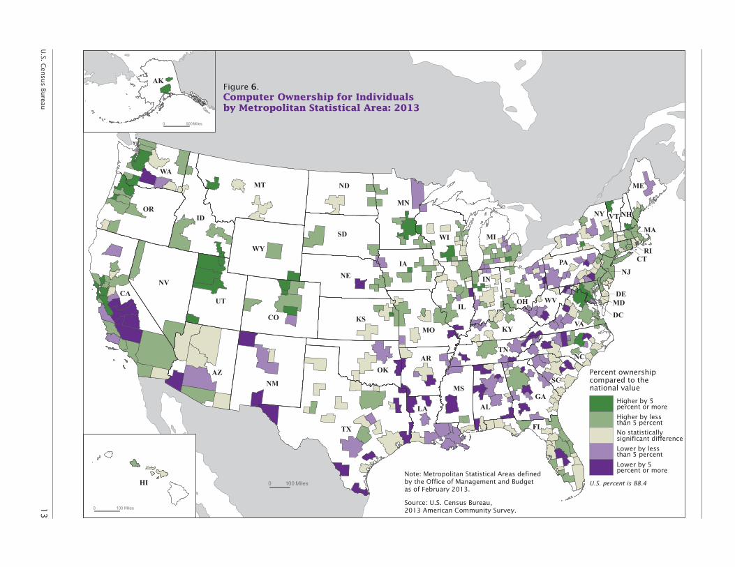
• Overall, 31 metropolitan areas had rates of com-puter ownership above the national average by at least 5 percentage points. Of these metropolitan areas, most were located in the West, while only 2 were located in the South (Figure 5).

9 Although the ACS gathers data for Puerto Rico, this report does not include discussion of those estimates.

Figure 1. 2013 ACS Computer and Internet Use Questions

Source: U.S. Census Bureau, 2013 American Community Survey.

U.S. Census Bureau 3

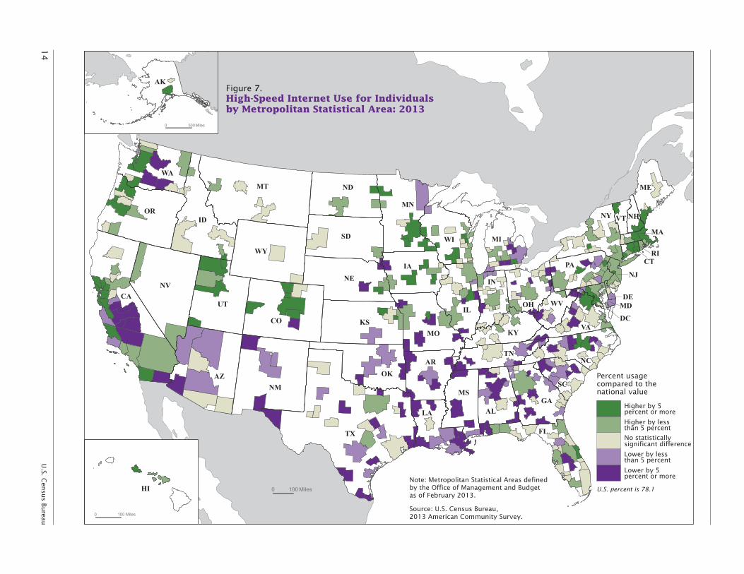
• Overall, 59 metropolitan areas had rates of high-speed Internet use above the national average by at least 5 percentage points. Of these metropoli-tan areas, 25 were located in the West, 17 in the Midwest, and 13 in the Northeast. Only 4 metro-politan areas in the South had high-speed Internet rates at least 5 percentage points above the national average (Figure 6).

CHARACTERISTICS OF HOUSEHOLD AND INDIVIDUAL COMPUTER AND INTERNET USE

Previous Census Bureau reports have examined data from the CPS to show that household computer owner-ship and Internet use have both increased steadily over

Table 1.Computer and Internet Use for Households: 2013(In thousands. For information on confidentiality protection, sampling error, nonsampling error, and definitions, see www.census.gov/acs/www)

Household characteristics

Total households

Household with a computer

Household with Internet use

Total

Desktop or laptop

computerHandheld computer

With some

Internet subscription1

With high-speed

Internet connection1

Total households . . . . . . . . . . . . . . . . . . . . . . . . 116,291 83 .8 78 .5 63 .6 74 .4 73 .4

Age of householder 15–34 years . . . . . . . . . . . . . . . . . . . . . . . . . . . . . . . . . 22,331 92 .1 82 .1 83 .3 77 .7 77 .4 35–44 years . . . . . . . . . . . . . . . . . . . . . . . . . . . . . . . . . 20,745 92 .5 86 .4 80 .7 82 .5 81 .9 45–64 years . . . . . . . . . . . . . . . . . . . . . . . . . . . . . . . . . 46,015 86 .8 82 .7 65 .2 78 .7 77 .6 65 years and older . . . . . . . . . . . . . . . . . . . . . . . . . . . . 27,201 65 .1 62 .3 31 .8 58 .3 56 .3

Race and Hispanic origin of householder White alone, non-Hispanic . . . . . . . . . . . . . . . . . . . . 80,699 85 .4 81 .4 63 .4 77 .4 76 .2 Black alone, non-Hispanic . . . . . . . . . . . . . . . . . . . . 13,816 75 .8 66 .3 58 .9 61 .3 60 .6 Asian alone, non-Hispanic . . . . . . . . . . . . . . . . . . . . 4,941 92 .5 90 .0 78 .6 86 .6 86 .0 Hispanic (of any race) . . . . . . . . . . . . . . . . . . . . . . . . . 14,209 79 .7 70 .0 63 .7 66 .7 65 .9

Limited English-speaking household No . . . . . . . . . . . . . . . . . . . . . . . . . . . . . . . . . . . . . . . . 111,084 84 .7 79 .6 64 .6 75 .5 74 .4 Yes . . . . . . . . . . . . . . . . . . . . . . . . . . . . . . . . . . . . . . . . 5,207 63 .9 54 .9 43 .7 51 .4 50 .6

Metropolitan status Metropolitan area . . . . . . . . . . . . . . . . . . . . . . . . . . . . . 98,607 85 .1 79 .9 65 .9 76 .1 75 .2 Nonmetropolitan area . . . . . . . . . . . . . . . . . . . . . . . . . 17,684 76 .5 70 .6 51 .1 64 .8 63 .1

Household income Less than $25,000 . . . . . . . . . . . . . . . . . . . . . . . . . . . . 27,605 62 .4 53 .9 39 .6 48 .4 47 .2 $25,000–$49,999 . . . . . . . . . . . . . . . . . . . . . . . . . . . . . 27,805 81 .1 74 .0 55 .2 69 .0 67 .6 $50,000–$99,999 . . . . . . . . . . . . . . . . . . . . . . . . . . . . . 34,644 92 .6 88 .4 71 .9 84 .9 83 .8 $100,000–$149,999 . . . . . . . . . . . . . . . . . . . . . . . . . . . 14,750 97 .1 95 .1 84 .5 92 .7 92 .1 $150,000 and more . . . . . . . . . . . . . . . . . . . . . . . . . . . 11,487 98 .1 96 .8 90 .2 94 .9 94 .5

Region Northeast . . . . . . . . . . . . . . . . . . . . . . . . . . . . . . . . . . . 20,937 84 .1 79 .9 62 .8 76 .8 76 .0 Midwest . . . . . . . . . . . . . . . . . . . . . . . . . . . . . . . . . . . . 26,161 83 .1 77 .9 61 .2 73 .4 72 .1 South . . . . . . . . . . . . . . . . . . . . . . . . . . . . . . . . . . . . . . 43,399 82 .2 76 .0 63 .2 71 .7 70 .7 West . . . . . . . . . . . . . . . . . . . . . . . . . . . . . . . . . . . . . . . 25,793 86 .8 82 .0 67 .4 78 .1 77 .1

Total 25 years and older . . . . . . . . . . . . . . . . . . . 111,700 83 .5 78 .5 62 .8 74 .5 73 .5

Educational attainment of householder Less than high school graduate . . . . . . . . . . . . . . . . . . 12,855 56 .0 47 .2 36 .5 43 .8 42 .7 High school graduate (includes equivalency) . . . . . . . . 28,277 73 .9 66 .9 48 .5 62 .9 61 .4 Some college or associate’s degree . . . . . . . . . . . . . . 34,218 89 .0 83 .9 67 .0 79 .2 78 .0 Bachelor’s degree or higher . . . . . . . . . . . . . . . . . . . . . 36,349 95 .5 93 .5 79 .3 90 .1 89 .4

1 About 4 .2 percent of all households reported household Internet use without a paid subscription . These households are not included in this table . Note: Handheld computers include smart mobile phones and other handheld wireless computers . High-speed Internet indicates a household has Internet

service type other than dial-up alone . For a version of Table 1 with margins of error, please see Appendix Table A at <www .census .gov/hhes/computer/> .Source: U .S . Census Bureau, 2013 American Community Survey .


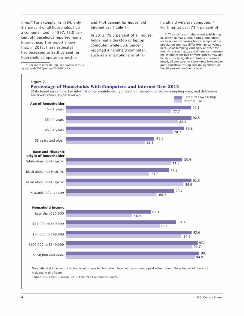
time.10 For example, in 1984, only 8.2 percent of all households had a computer, and in 1997, 18.0 per-cent of households reported home Internet use. This report shows that, in 2013, these estimates had increased to 83.8 percent for household computer ownership

10 For more information, see <www.census .gov/prod/2013pubs/p20-569.pdf>.

and 74.4 percent for household Internet use (Table 1).

In 2013, 78.5 percent of all house-holds had a desktop or laptop computer, while 63.6 percent reported a handheld computer, such as a smartphone or other

handheld wireless computer.11 For Internet use, 73.4 percent of

11 The estimates in this report (which may be shown in maps, text, figures, and tables) are based on responses from a sample of the population and may differ from actual values because of sampling variability or other fac-tors. As a result, apparent differences between the estimates for two or more groups may not be statistically significant. Unless otherwise noted, all comparative statements have under-gone statistical testing and are significant at the 90 percent confidence level.

Figure 2. Percentage of Households With Computers and Internet Use: 2013(Data based on sample. For information on confidentiality protection, sampling error, nonsampling error, and definitions, see www.census.gov/acs/www/)

Note: About 4.2 percent of all households reported household Internet use without a paid subscription. These households are not

included in this figure.


Computer ownershipInternet use

92.582.5

65.158.3

85.477.4

75.861.3

92.586.6

79.766.7

62.448.4

81.169.0

92.684.9

97.192.7

98.194.9

86.878.7

Age of householder

Household income

Race and Hispanicorigin of householder

77.792.1

$150,000 and more

$100,000 to $149,999

$50,000 to $99,999

$25,000 to $49,999

Less than $25,000

Hispanic (of any race)

Asian alone non-Hispanic

Black alone non-Hispanic

White alone non-Hispanic

65 years and older

45–64 years

35–44 years

15–34 years


households reported a high-speed Internet connection.12

Although household computer ownership was consistently higher than household Internet use, both followed similar patterns across demographic groups. For example, computer ownership and Internet use were most common in homes with relatively young household-ers, and both indicators dropped off steeply as a householder’s age increased. Figure 2 shows that 92.5 percent of homes with a house-holder aged 35 to 44 had a com-puter, compared with 65.1 percent of homes with a householder aged 65 or older. Similarly, 82.5 percent of homes with a householder aged 35 to 44 reported Internet use, compared with 58.3 percent with a householder aged 65 or older.

Similar differences were observed for race and Hispanic-origin groups, as computer ownership and Internet use were less common in Black and Hispanic households than in White and Asian households.13 In 2013, 75.8 percent of homes with a Black householder and 79.7 percent of homes with a Hispanic householder reported computer ownership, com-pared with 85.4 percent of homes with a White householder and 92.5

12 High-speed Internet use indicates that a household has an Internet service type other than dial-up alone. This includes DSL, cable modem, fiber-optic, mobile broadband, and satellite Internet services.

13 Federal surveys now give respondents the option of reporting more than one race. Therefore, two basic ways of defining a race group are possible. A group such as Asian may be defined as those who reported Asian and no other race (the race-alone or single-race concept) or as those who reported Asian regardless of whether they also reported another race (the race-alone-or-in-combination concept). The body of this report (text, fig-ures, and text tables) shows data for people who reported they were the single race White and not Hispanic, people who reported the single race Black and not Hispanic, and people who reported the single race Asian and not Hispanic. Use of the single-race popu-lations does not imply that it is the preferred method of presenting or analyzing data.

percent of homes with an Asian householder. Similar differences existed for home Internet use, with Black householders (61.3 percent) and Hispanic householders (66.7 percent) reporting Internet use at lower levels than White householders (77.4 percent) and Asian householders (86.6 percent).14

Other groups reported consistently lower levels of both computer ownership and Internet use as well, including households with low incomes, those located outside of metropolitan areas, and homes where the householder reported a relatively low level of educational attainment. The contrast between regions was not particularly large, but households in the West did have the highest rates of both computer ownership (86.8 percent) and Internet use (78.1 percent), while households in the South had the lowest rates on both indicators (82.2 percent for computer ownership and 71.7 percent for Internet use).

Patterns for individuals were similar to those observed for households, with computer ownership and Internet use tending to be high-est among the young, Whites and Asians, and the highly educated (Table 2). Individual computer own-ership and Internet use were also strongly associated with disability status, as individuals without a disability were more likely to report living in a home with computer ownership (90.4 percent) and Internet use (81.1 percent) than individuals with disabilities, 73.9 percent of whom reported house-hold computer ownership and 63.8 percent of whom reported living in a home with Internet use.

Not surprisingly, labor force status also impacted rates of computer

14 For both computer ownership and Inter-net use, Asian household rates were statisti-cally higher than for White households.

ownership and Internet use among individuals, as employed people reported household computer own-ership (92.7 percent) and house-hold Internet use (84.1 percent) more frequently than the unem-ployed (87.1 percent for computer ownership and 74.2 percent for Internet use, respectively).

TYPE OF INTERNET CONNECTION

Just as with computer owner-ship and Internet use, household level differences existed for the methods that households used to access the Internet.

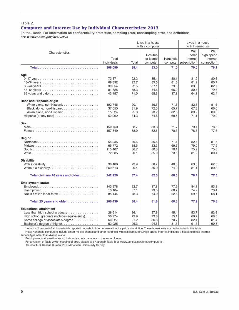
The most common household connection type was via a cable modem (42.8 percent), followed by mobile broadband (33.1 per-cent), and DSL connections (21.2 percent). About one-quarter of all households had no paid Internet subscription at all, while only 1.0 percent of all households reported connecting to the Internet using a dial-up connection (Figure 3).15, 16

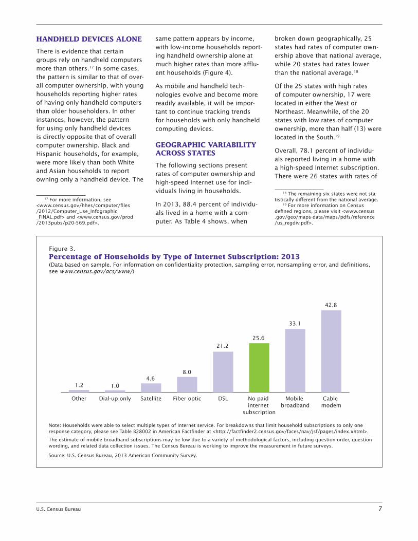
Variation also existed across groups for the types of connections people used to go online, but in general, these patterns were similar to overall computer ownership and Internet use trends. For example, among users of the most common type of Internet connection, cable modem service, use tended to be highest among the young, Whites or Asians, and the affluent, just as with overall computer ownership and Internet use (Table 3).

15 The estimate of no Internet includes households without any Internet use at home and households connecting without a paid subscription.

16 Dial-up service uses a regular telephone line to connect to the Internet and does not allow users to be online and use the phone at the same time.


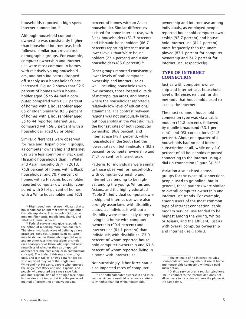
Table 2.Computer and Internet Use by Individual Characteristics: 2013(In thousands. For information on confidentiality protection, sampling error, nonsampling error, and definitions, see www.census.gov/acs/www)

Characteristics

Total individuals

Lives in a house with a computer

Lives in a house with Internet use

Total

Desktop or laptop computer

Handheld computer

With some

Internet subscription1

With high-speed

Internet connection1

Total . . . . . . . . . . . . . . . . . . . . . . . . . . . . . . . . . . . 308,099 88 .4 83 .0 71 .0 79 .0 78 .1

Age 0–17 years . . . . . . . . . . . . . . . . . . . . . . . . . . . . . . . . . . 73,371 92 .2 85 .1 80 .1 81 .2 80 .6 18–34 years . . . . . . . . . . . . . . . . . . . . . . . . . . . . . . . . . 69,892 92 .7 85 .5 81 .6 81 .2 80 .7 35–44 years . . . . . . . . . . . . . . . . . . . . . . . . . . . . . . . . . 39,854 92 .5 87 .1 79 .8 83 .3 82 .7 45–64 years . . . . . . . . . . . . . . . . . . . . . . . . . . . . . . . . . 81,825 88 .3 84 .5 66 .9 80 .6 79 .6 65 years and older . . . . . . . . . . . . . . . . . . . . . . . . . . . . 43,157 71 .0 68 .3 37 .8 64 .3 62 .4

Race and Hispanic origin White alone, non-Hispanic . . . . . . . . . . . . . . . . . . . . 192,745 90 .1 86 .5 71 .5 82 .5 81 .6 Black alone, non-Hispanic . . . . . . . . . . . . . . . . . . . . 37,055 81 .9 72 .5 65 .7 67 .3 66 .6 Asian alone, non-Hispanic . . . . . . . . . . . . . . . . . . . . 15,524 95 .3 93 .2 82 .5 89 .9 89 .3 Hispanic (of any race) . . . . . . . . . . . . . . . . . . . . . . . . . 52,992 84 .3 74 .6 68 .5 71 .1 70 .2

Sex Male . . . . . . . . . . . . . . . . . . . . . . . . . . . . . . . . . . . . . . . 150,750 88 .7 83 .3 71 .7 79 .4 78 .5 Female . . . . . . . . . . . . . . . . . . . . . . . . . . . . . . . . . . . . . 157,349 88 .0 82 .6 70 .3 78 .5 77 .6

Region Northeast . . . . . . . . . . . . . . . . . . . . . . . . . . . . . . . . . . . 54,235 89 .5 85 .5 71 .1 82 .5 81 .7 Midwest . . . . . . . . . . . . . . . . . . . . . . . . . . . . . . . . . . . . 65,772 88 .5 83 .3 69 .6 79 .0 77 .9 South . . . . . . . . . . . . . . . . . . . . . . . . . . . . . . . . . . . . . . 115,407 86 .7 80 .3 70 .1 75 .9 75 .0 West . . . . . . . . . . . . . . . . . . . . . . . . . . . . . . . . . . . . . . . 72,685 90 .1 85 .0 73 .5 81 .2 80 .4

Disability With a disability . . . . . . . . . . . . . . . . . . . . . . . . . . . . . . 38,486 73 .9 68 .7 48 .3 63 .8 62 .5 Without a disability . . . . . . . . . . . . . . . . . . . . . . . . . . . . 269,613 90 .4 85 .0 74 .2 81 .1 80 .3

Total civilians 16 years and older . . . . . . . . . . . 242,226 87 .4 82 .5 68 .5 78 .4 77 .5

Employment status Employed . . . . . . . . . . . . . . . . . . . . . . . . . . . . . . . . . . . 143,978 92 .7 87 .8 77 .9 84 .1 83 .3 Unemployed . . . . . . . . . . . . . . . . . . . . . . . . . . . . . . . . . 13,104 87 .1 79 .5 68 .7 74 .2 73 .4 Not in civilian labor force . . . . . . . . . . . . . . . . . . . . . . . 85,144 78 .3 74 .0 52 .6 69 .5 68 .1

Total 25 years and older . . . . . . . . . . . . . . . . . . 206,439 86 .4 81 .8 66 .3 77 .9 76 .8

Educational attainment Less than high school graduate . . . . . . . . . . . . . . . . . . 26,914 66 .1 57 .6 45 .4 53 .7 52 .6 High school graduate (includes equivalency) . . . . . . . . 56,974 79 .9 73 .8 55 .1 69 .7 68 .3 Some college or associate’s degree . . . . . . . . . . . . . . 60,527 91 .2 86 .8 70 .7 82 .4 81 .4 Bachelor’s degree or higher . . . . . . . . . . . . . . . . . . . . . 62,025 96 .3 94 .6 81 .5 91 .5 90 .8

1 About 4 .2 percent of all households reported household Internet use without a paid subscription . These households are not included in this table . Note: Handheld computers include smart mobile phones and other handheld wireless computers . High-speed Internet indicates a household has Internet

service type other than dial-up alone . Employment status estimates exclude active duty members of the armed forces .For a version of Table 2 with margins of error, please see Appendix Table B at <www .census .gov/hhes/computer/> . Source: U .S . Census Bureau, 2013 American Community Survey .


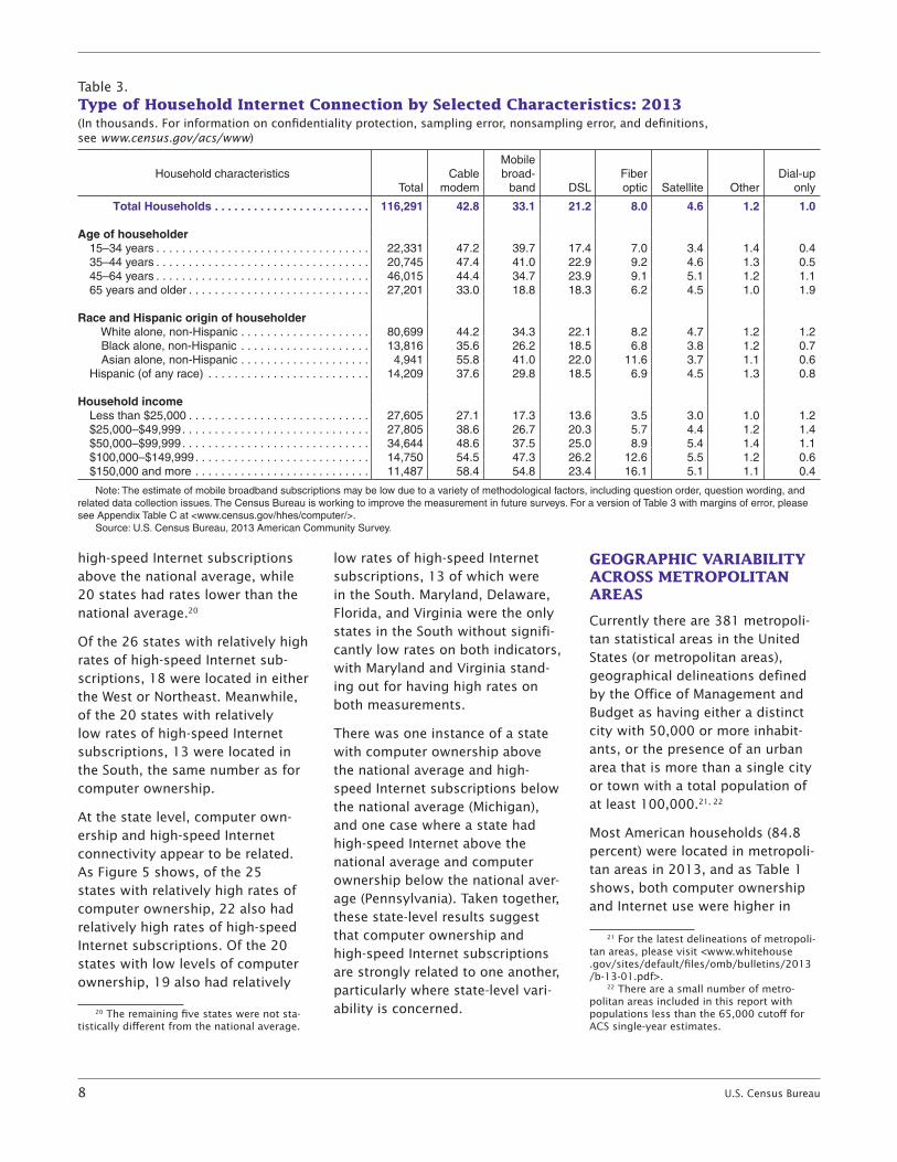
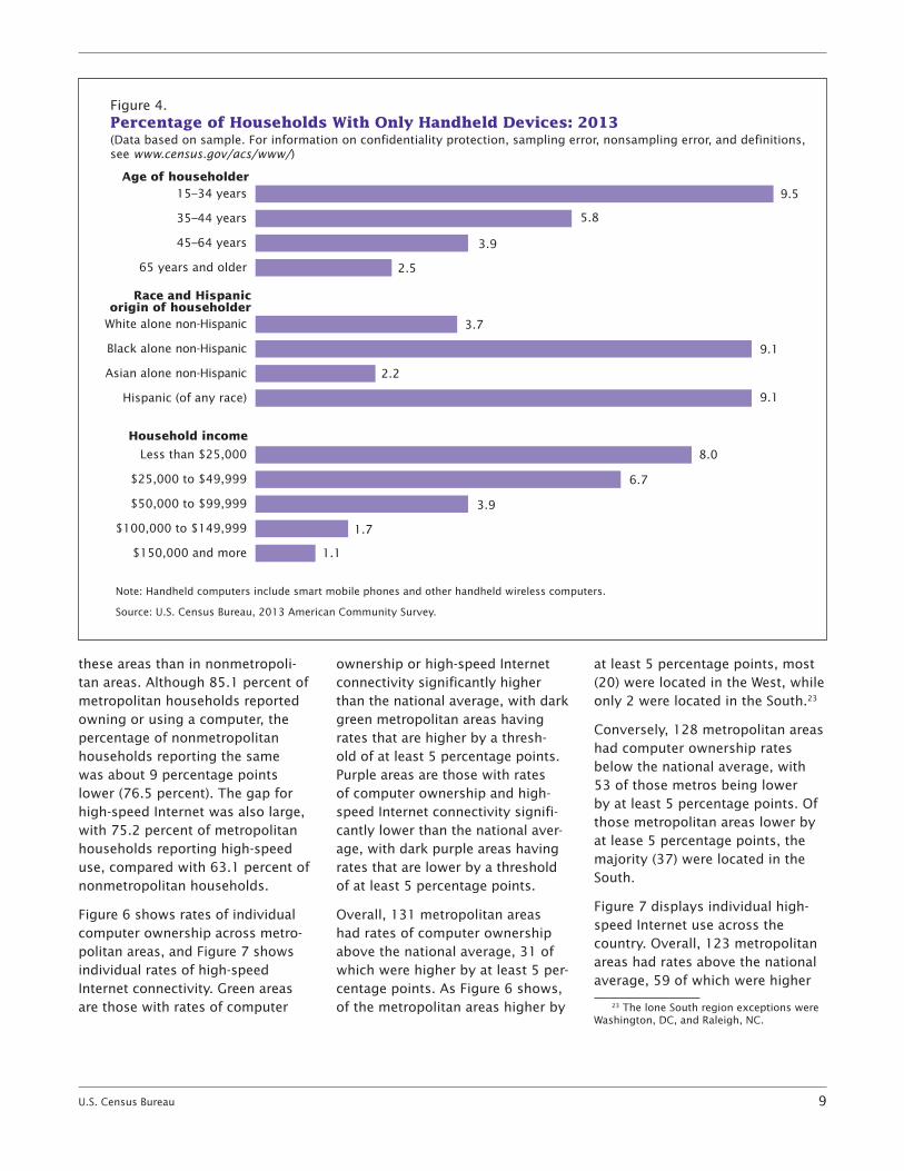
HANDHELD DEVICES ALONE

There is evidence that certain groups rely on handheld computers more than others.17 In some cases, the pattern is similar to that of over-all computer ownership, with young households reporting higher rates of having only handheld computers than older householders. In other instances, however, the pattern for using only handheld devices is directly opposite that of overall computer ownership. Black and Hispanic households, for example, were more likely than both White and Asian households to report owning only a handheld device. The

17 For more information, see <www.census.gov/hhes/computer/files /2012/Computer_Use_Infographic _FINAL.pdf> and <www.census.gov/prod /2013pubs/p20-569.pdf>.

same pattern appears by income, with low-income households report-ing handheld ownership alone at much higher rates than more afflu-ent households (Figure 4).

As mobile and handheld tech-nologies evolve and become more readily available, it will be impor-tant to continue tracking trends for households with only handheld computing devices.

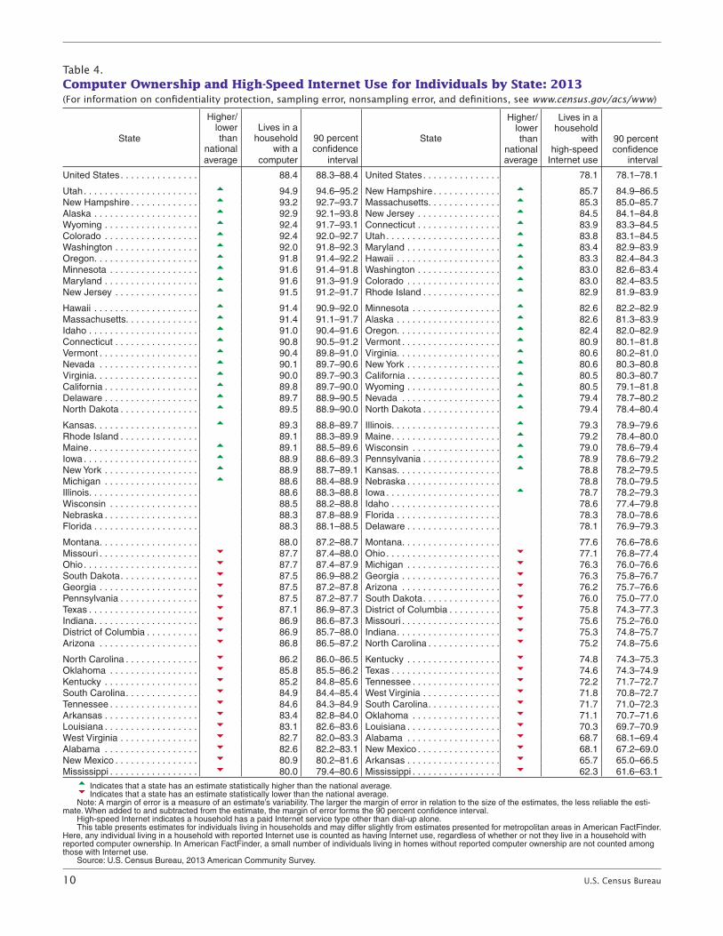
GEOGRAPHIC VARIABILITY ACROSS STATES

The following sections present rates of computer ownership and high-speed Internet use for indi-viduals living in households.

In 2013, 88.4 percent of individu-als lived in a home with a com-puter. As Table 4 shows, when

broken down geographically, 25 states had rates of computer own-ership above that national average, while 20 states had rates lower than the national average.18

Of the 25 states with high rates of computer ownership, 17 were located in either the West or Northeast. Meanwhile, of the 20 states with low rates of computer ownership, more than half (13) were located in the South.19

Overall, 78.1 percent of individu-als reported living in a home with a high-speed Internet subscription. There were 26 states with rates of

18 The remaining six states were not sta-tistically different from the national average.

19 For more information on Census defined regions, please visit <www.census .gov/geo/maps-data/maps/pdfs/reference /us_regdiv.pdf>.

Figure 3. Percentage of Households by Type of Internet Subscription: 2013(Data based on sample. For information on confidentiality protection, sampling error, nonsampling error, and definitions, see www.census.gov/acs/www/)

8.0

1.01.24.6

33.1

25.621.2

42.8

Cable modem

Mobile broadband

No paid internet

subscription

DSLFiber opticSatelliteDial-up onlyOther

Note: Households were able to select multiple types of Internet service. For breakdowns that limit household subscriptions to only one response category, please see Table B28002 in American Factfinder at <http://factfinder2.census.gov/faces/nav/jsf/pages/index.xhtml>.

The estimate of mobile broadband subscriptions may be low due to a variety of methodological factors, including question order, question wording, and related data collection issues. The Census Bureau is working to improve the measurement in future surveys.



high-speed Internet subscriptions above the national average, while 20 states had rates lower than the national average.20

Of the 26 states with relatively high rates of high-speed Internet sub-scriptions, 18 were located in either the West or Northeast. Meanwhile, of the 20 states with relatively low rates of high-speed Internet subscriptions, 13 were located in the South, the same number as for computer ownership.

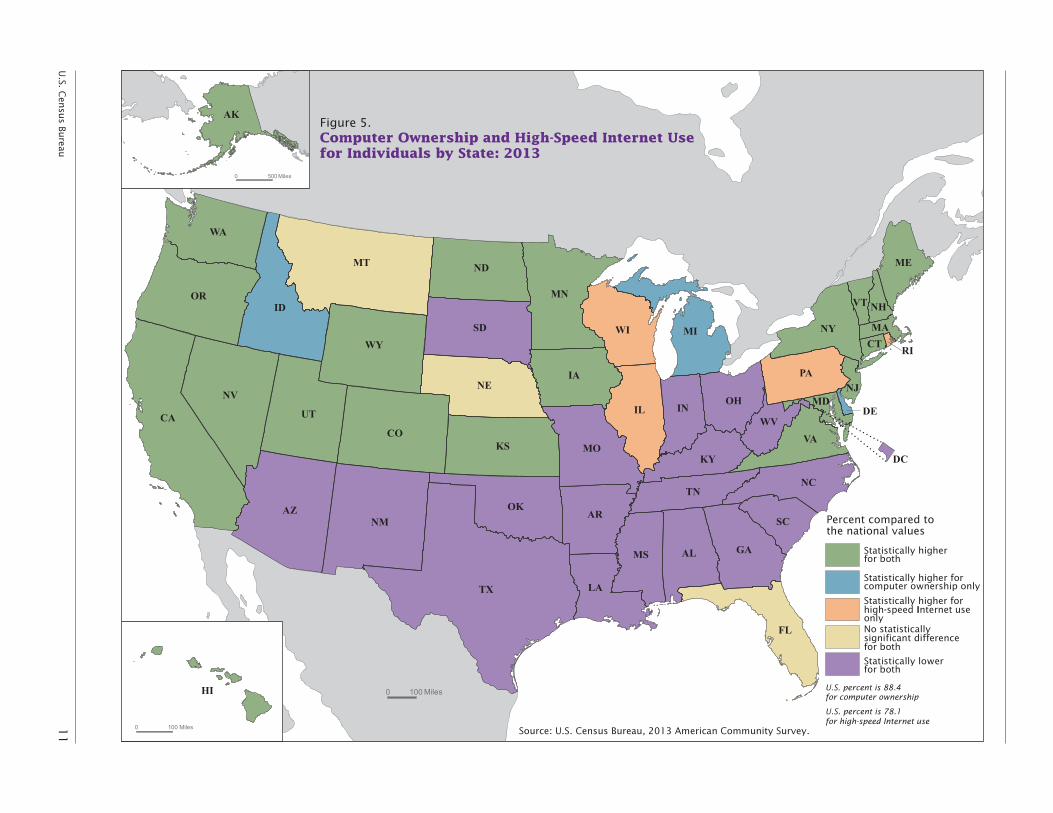
At the state level, computer own-ership and high-speed Internet connectivity appear to be related. As Figure 5 shows, of the 25 states with relatively high rates of computer ownership, 22 also had relatively high rates of high-speed Internet subscriptions. Of the 20 states with low levels of computer ownership, 19 also had relatively

20 The remaining five states were not sta-tistically different from the national average.

low rates of high-speed Internet subscriptions, 13 of which were in the South. Maryland, Delaware, Florida, and Virginia were the only states in the South without signifi-cantly low rates on both indicators, with Maryland and Virginia stand-ing out for having high rates on both measurements.

There was one instance of a state with computer ownership above the national average and high-speed Internet subscriptions below the national average (Michigan), and one case where a state had high-speed Internet above the national average and computer ownership below the national aver-age (Pennsylvania). Taken together, these state-level results suggest that computer ownership and high-speed Internet subscriptions are strongly related to one another, particularly where state-level vari-ability is concerned.

GEOGRAPHIC VARIABILITY ACROSS METROPOLITAN AREAS

Currently there are 381 metropoli-tan statistical areas in the United States (or metropolitan areas), geographical delineations defined by the Office of Management and Budget as having either a distinct city with 50,000 or more inhabit-ants, or the presence of an urban area that is more than a single city or town with a total population of at least 100,000.21, 22

Most American households (84.8 percent) were located in metropoli-tan areas in 2013, and as Table 1 shows, both computer ownership and Internet use were higher in

21 For the latest delineations of metropoli-tan areas, please visit <www.whitehouse .gov/sites/default/files/omb/bulletins/2013 /b-13-01.pdf>.

22 There are a small number of metro-politan areas included in this report with populations less than the 65,000 cutoff for ACS single-year estimates.

Table 3. Type of Household Internet Connection by Selected Characteristics: 2013(In thousands. For information on confidentiality protection, sampling error, nonsampling error, and definitions, see www.census.gov/acs/www)

Household characteristicsTotal

Cable modem

Mobile broad-

band DSLFiber optic Satellite Other

Dial-up only

Total Households . . . . . . . . . . . . . . . . . . . . . . . . 116,291 42 .8 33 .1 21 .2 8 .0 4 .6 1 .2 1 .0

Age of householder 15–34 years . . . . . . . . . . . . . . . . . . . . . . . . . . . . . . . . . 22,331 47 .2 39 .7 17 .4 7 .0 3 .4 1 .4 0 .4 35–44 years . . . . . . . . . . . . . . . . . . . . . . . . . . . . . . . . . 20,745 47 .4 41 .0 22 .9 9 .2 4 .6 1 .3 0 .5 45–64 years . . . . . . . . . . . . . . . . . . . . . . . . . . . . . . . . . 46,015 44 .4 34 .7 23 .9 9 .1 5 .1 1 .2 1 .1 65 years and older . . . . . . . . . . . . . . . . . . . . . . . . . . . . 27,201 33 .0 18 .8 18 .3 6 .2 4 .5 1 .0 1 .9

Race and Hispanic origin of householder White alone, non-Hispanic . . . . . . . . . . . . . . . . . . . . 80,699 44 .2 34 .3 22 .1 8 .2 4 .7 1 .2 1 .2 Black alone, non-Hispanic . . . . . . . . . . . . . . . . . . . . 13,816 35 .6 26 .2 18 .5 6 .8 3 .8 1 .2 0 .7 Asian alone, non-Hispanic . . . . . . . . . . . . . . . . . . . . 4,941 55 .8 41 .0 22 .0 11 .6 3 .7 1 .1 0 .6 Hispanic (of any race) . . . . . . . . . . . . . . . . . . . . . . . . . 14,209 37 .6 29 .8 18 .5 6 .9 4 .5 1 .3 0 .8

Household income Less than $25,000 . . . . . . . . . . . . . . . . . . . . . . . . . . . . 27,605 27 .1 17 .3 13 .6 3 .5 3 .0 1 .0 1 .2 $25,000–$49,999 . . . . . . . . . . . . . . . . . . . . . . . . . . . . . 27,805 38 .6 26 .7 20 .3 5 .7 4 .4 1 .2 1 .4 $50,000–$99,999 . . . . . . . . . . . . . . . . . . . . . . . . . . . . . 34,644 48 .6 37 .5 25 .0 8 .9 5 .4 1 .4 1 .1 $100,000–$149,999 . . . . . . . . . . . . . . . . . . . . . . . . . . . 14,750 54 .5 47 .3 26 .2 12 .6 5 .5 1 .2 0 .6 $150,000 and more . . . . . . . . . . . . . . . . . . . . . . . . . . . 11,487 58 .4 54 .8 23 .4 16 .1 5 .1 1 .1 0 .4

Note: The estimate of mobile broadband subscriptions may be low due to a variety of methodological factors, including question order, question wording, and related data collection issues . The Census Bureau is working to improve the measurement in future surveys . For a version of Table 3 with margins of error, please see Appendix Table C at <www .census .gov/hhes/computer/> .

Source: U .S . Census Bureau, 2013 American Community Survey .


these areas than in nonmetropoli-tan areas. Although 85.1 percent of metropolitan households reported owning or using a computer, the percentage of nonmetropolitan households reporting the same was about 9 percentage points lower (76.5 percent). The gap for high-speed Internet was also large, with 75.2 percent of metropolitan households reporting high-speed use, compared with 63.1 percent of nonmetropolitan households.

Figure 6 shows rates of individual computer ownership across metro-politan areas, and Figure 7 shows individual rates of high-speed Internet connectivity. Green areas are those with rates of computer

ownership or high-speed Internet connectivity significantly higher than the national average, with dark green metropolitan areas having rates that are higher by a thresh-old of at least 5 percentage points. Purple areas are those with rates of computer ownership and high-speed Internet connectivity signifi-cantly lower than the national aver-age, with dark purple areas having rates that are lower by a threshold of at least 5 percentage points.

Overall, 131 metropolitan areas had rates of computer ownership above the national average, 31 of which were higher by at least 5 per-centage points. As Figure 6 shows, of the metropolitan areas higher by

at least 5 percentage points, most (20) were located in the West, while only 2 were located in the South.23

Conversely, 128 metropolitan areas had computer ownership rates below the national average, with 53 of those metros being lower by at least 5 percentage points. Of those metropolitan areas lower by at lease 5 percentage points, the majority (37) were located in the South.

Figure 7 displays individual high-speed Internet use across the country. Overall, 123 metropolitan areas had rates above the national average, 59 of which were higher

23 The lone South region exceptions were Washington, DC, and Raleigh, NC.

Figure 4. Percentage of Households With Only Handheld Devices: 2013(Data based on sample. For information on confidentiality protection, sampling error, nonsampling error, and definitions, see www.census.gov/acs/www/)

3.9

2.5

9.1

3.7

2.2

9.1

8.0

6.7

3.9

1.7

1.1

5.8

9.5

$150,000 and more

$100,000 to $149,999

$50,000 to $99,999

$25,000 to $49,999

Less than $25,000

Hispanic (of any race)

Asian alone non-Hispanic

Black alone non-Hispanic

White alone non-Hispanic

65 years and older

45–64 years

35–44 years

15–34 years

Note: Handheld computers include smart mobile phones and other handheld wireless computers.


Age of householder

Household income

Race and Hispanicorigin of householder


Table 4. Computer Ownership and High-Speed Internet Use for Individuals by State: 2013(For information on confidentiality protection, sampling error, nonsampling error, and definitions, see www.census.gov/acs/www)

State

Higher/lower than

national average

Lives in a household

with a computer

90 percent confidence

interval

State

Higher/lower than

national average

Lives in a household

with high-speed

Internet use

90 percent confidence

interval

United States . . . . . . . . . . . . . . . 88 .4 88 .3–88 .4 United States . . . . . . . . . . . . . . . 78 .1 78 .1–78 .1

Utah . . . . . . . . . . . . . . . . . . . . . . 94 .9 94 .6–95 .2 New Hampshire . . . . . . . . . . . . . 85 .7 84 .9–86 .5New Hampshire . . . . . . . . . . . . . 93 .2 92 .7–93 .7 Massachusetts . . . . . . . . . . . . . . 85 .3 85 .0–85 .7Alaska . . . . . . . . . . . . . . . . . . . . 92 .9 92 .1–93 .8 New Jersey . . . . . . . . . . . . . . . . 84 .5 84 .1–84 .8Wyoming . . . . . . . . . . . . . . . . . . 92 .4 91 .7–93 .1 Connecticut . . . . . . . . . . . . . . . . 83 .9 83 .3–84 .5Colorado . . . . . . . . . . . . . . . . . . 92 .4 92 .0–92 .7 Utah . . . . . . . . . . . . . . . . . . . . . . 83 .8 83 .1–84 .5Washington . . . . . . . . . . . . . . . . 92 .0 91 .8–92 .3 Maryland . . . . . . . . . . . . . . . . . . 83 .4 82 .9–83 .9Oregon . . . . . . . . . . . . . . . . . . . . 91 .8 91 .4–92 .2 Hawaii . . . . . . . . . . . . . . . . . . . . 83 .3 82 .4–84 .3Minnesota . . . . . . . . . . . . . . . . . 91 .6 91 .4–91 .8 Washington . . . . . . . . . . . . . . . . 83 .0 82 .6–83 .4Maryland . . . . . . . . . . . . . . . . . . 91 .6 91 .3–91 .9 Colorado . . . . . . . . . . . . . . . . . . 83 .0 82 .4–83 .5New Jersey . . . . . . . . . . . . . . . . 91 .5 91 .2–91 .7 Rhode Island . . . . . . . . . . . . . . . 82 .9 81 .9–83 .9

Hawaii . . . . . . . . . . . . . . . . . . . . 91 .4 90 .9–92 .0 Minnesota . . . . . . . . . . . . . . . . . 82 .6 82 .2–82 .9Massachusetts . . . . . . . . . . . . . . 91 .4 91 .1–91 .7 Alaska . . . . . . . . . . . . . . . . . . . . 82 .6 81 .3–83 .9Idaho . . . . . . . . . . . . . . . . . . . . . 91 .0 90 .4–91 .6 Oregon . . . . . . . . . . . . . . . . . . . . 82 .4 82 .0–82 .9Connecticut . . . . . . . . . . . . . . . . 90 .8 90 .5–91 .2 Vermont . . . . . . . . . . . . . . . . . . . 80 .9 80 .1–81 .8Vermont . . . . . . . . . . . . . . . . . . . 90 .4 89 .8–91 .0 Virginia . . . . . . . . . . . . . . . . . . . . 80 .6 80 .2–81 .0Nevada . . . . . . . . . . . . . . . . . . . 90 .1 89 .7–90 .6 New York . . . . . . . . . . . . . . . . . . 80 .6 80 .3–80 .8Virginia . . . . . . . . . . . . . . . . . . . . 90 .0 89 .7–90 .3 California . . . . . . . . . . . . . . . . . . 80 .5 80 .3–80 .7California . . . . . . . . . . . . . . . . . . 89 .8 89 .7–90 .0 Wyoming . . . . . . . . . . . . . . . . . . 80 .5 79 .1–81 .8Delaware . . . . . . . . . . . . . . . . . . 89 .7 88 .9–90 .5 Nevada . . . . . . . . . . . . . . . . . . . 79 .4 78 .7–80 .2North Dakota . . . . . . . . . . . . . . . 89 .5 88 .9–90 .0 North Dakota . . . . . . . . . . . . . . . 79 .4 78 .4–80 .4

Kansas . . . . . . . . . . . . . . . . . . . . 89 .3 88 .8–89 .7 Illinois . . . . . . . . . . . . . . . . . . . . . 79 .3 78 .9–79 .6Rhode Island . . . . . . . . . . . . . . . 89 .1 88 .3–89 .9 Maine . . . . . . . . . . . . . . . . . . . . . 79 .2 78 .4–80 .0Maine . . . . . . . . . . . . . . . . . . . . . 89 .1 88 .5–89 .6 Wisconsin . . . . . . . . . . . . . . . . . 79 .0 78 .6–79 .4Iowa . . . . . . . . . . . . . . . . . . . . . . 88 .9 88 .6–89 .3 Pennsylvania . . . . . . . . . . . . . . . 78 .9 78 .6–79 .2New York . . . . . . . . . . . . . . . . . . 88 .9 88 .7–89 .1 Kansas . . . . . . . . . . . . . . . . . . . . 78 .8 78 .2–79 .5Michigan . . . . . . . . . . . . . . . . . . 88 .6 88 .4–88 .9 Nebraska . . . . . . . . . . . . . . . . . . 78 .8 78 .0–79 .5Illinois . . . . . . . . . . . . . . . . . . . . . 88 .6 88 .3–88 .8 Iowa . . . . . . . . . . . . . . . . . . . . . . 78 .7 78 .2–79 .3Wisconsin . . . . . . . . . . . . . . . . . 88 .5 88 .2–88 .8 Idaho . . . . . . . . . . . . . . . . . . . . . 78 .6 77 .4–79 .8Nebraska . . . . . . . . . . . . . . . . . . 88 .3 87 .8–88 .9 Florida . . . . . . . . . . . . . . . . . . . . 78 .3 78 .0–78 .6Florida . . . . . . . . . . . . . . . . . . . . 88 .3 88 .1–88 .5 Delaware . . . . . . . . . . . . . . . . . . 78 .1 76 .9–79 .3

Montana . . . . . . . . . . . . . . . . . . . 88 .0 87 .2–88 .7 Montana . . . . . . . . . . . . . . . . . . . 77 .6 76 .6–78 .6Missouri . . . . . . . . . . . . . . . . . . . 87 .7 87 .4–88 .0 Ohio . . . . . . . . . . . . . . . . . . . . . . 77 .1 76 .8–77 .4Ohio . . . . . . . . . . . . . . . . . . . . . . 87 .7 87 .4–87 .9 Michigan . . . . . . . . . . . . . . . . . . 76 .3 76 .0–76 .6South Dakota . . . . . . . . . . . . . . . 87 .5 86 .9–88 .2 Georgia . . . . . . . . . . . . . . . . . . . 76 .3 75 .8–76 .7Georgia . . . . . . . . . . . . . . . . . . . 87 .5 87 .2–87 .8 Arizona . . . . . . . . . . . . . . . . . . . 76 .2 75 .7–76 .6Pennsylvania . . . . . . . . . . . . . . . 87 .5 87 .2–87 .7 South Dakota . . . . . . . . . . . . . . . 76 .0 75 .0–77 .0Texas . . . . . . . . . . . . . . . . . . . . . 87 .1 86 .9–87 .3 District of Columbia . . . . . . . . . . 75 .8 74 .3–77 .3Indiana . . . . . . . . . . . . . . . . . . . . 86 .9 86 .6–87 .3 Missouri . . . . . . . . . . . . . . . . . . . 75 .6 75 .2–76 .0District of Columbia . . . . . . . . . . 86 .9 85 .7–88 .0 Indiana . . . . . . . . . . . . . . . . . . . . 75 .3 74 .8–75 .7Arizona . . . . . . . . . . . . . . . . . . . 86 .8 86 .5–87 .2 North Carolina . . . . . . . . . . . . . . 75 .2 74 .8–75 .6

North Carolina . . . . . . . . . . . . . . 86 .2 86 .0–86 .5 Kentucky . . . . . . . . . . . . . . . . . . 74 .8 74 .3–75 .3Oklahoma . . . . . . . . . . . . . . . . . 85 .8 85 .5–86 .2 Texas . . . . . . . . . . . . . . . . . . . . . 74 .6 74 .3–74 .9Kentucky . . . . . . . . . . . . . . . . . . 85 .2 84 .8–85 .6 Tennessee . . . . . . . . . . . . . . . . . 72 .2 71 .7–72 .7South Carolina . . . . . . . . . . . . . . 84 .9 84 .4–85 .4 West Virginia . . . . . . . . . . . . . . . 71 .8 70 .8–72 .7Tennessee . . . . . . . . . . . . . . . . . 84 .6 84 .3–84 .9 South Carolina . . . . . . . . . . . . . . 71 .7 71 .0–72 .3Arkansas . . . . . . . . . . . . . . . . . . 83 .4 82 .8–84 .0 Oklahoma . . . . . . . . . . . . . . . . . 71 .1 70 .7–71 .6Louisiana . . . . . . . . . . . . . . . . . . 83 .1 82 .6–83 .6 Louisiana . . . . . . . . . . . . . . . . . . 70 .3 69 .7–70 .9West Virginia . . . . . . . . . . . . . . . 82 .7 82 .0–83 .3 Alabama . . . . . . . . . . . . . . . . . . 68 .7 68 .1–69 .4Alabama . . . . . . . . . . . . . . . . . . 82 .6 82 .2–83 .1 New Mexico . . . . . . . . . . . . . . . . 68 .1 67 .2–69 .0New Mexico . . . . . . . . . . . . . . . . 80 .9 80 .2–81 .6 Arkansas . . . . . . . . . . . . . . . . . . 65 .7 65 .0–66 .5Mississippi . . . . . . . . . . . . . . . . . 80 .0 79 .4–80 .6 Mississippi . . . . . . . . . . . . . . . . . 62 .3 61 .6–63 .1

Indicates that a state has an estimate statistically higher than the national average . Indicates that a state has an estimate statistically lower than the national average . Note: A margin of error is a measure of an estimate’s variability . The larger the margin of error in relation to the size of the estimates, the less reliable the esti-

mate . When added to and subtracted from the estimate, the margin of error forms the 90 percent confidence interval .High-speed Internet indicates a household has a paid Internet service type other than dial-up alone .This table presents estimates for individuals living in households and may differ slightly from estimates presented for metropolitan areas in American FactFinder .

Here, any individual living in a household with reported Internet use is counted as having Internet use, regardless of whether or not they live in a household with reported computer ownership . In American FactFinder, a small number of individuals living in homes without reported computer ownership are not counted among those with Internet use .


U.S. C

ensu

s Bureau

1

1

!!

!!

!!

!!

!!

!!

!!

!!

!

!!

!

!

!

!

!

!

!

!

!

!

!

!

!

!

!

!

!

!

!

RI

DE

MA

MDNJ

CT

NHVT

WV

ME

SC

OH

KY

VA

TN

MI

MS

IN

NY

LA

NC

PA

AR

AL GA

WI

MO

WA

OK

FL

ND

IA

MN

IL

NE

WYSD

UT

KS

OR

CO

NM

ID

NV

AZ

MT

CA

TX

DC

AK

HI

0 500 Miles

0 100 Miles

0 100 Miles

Figure 5.Computer Ownership and High-Speed Internet Use for Individuals by State: 2013

Percent compared to the national values

Statistically higher forcomputer ownership only

Statistically higher for high-speed Internet use onlyNo statisticallysignificant differencefor both

Statistically higherfor both

Statistically lowerfor both

U.S. percent is 88.4 for computer ownership

U.S. percent is 78.1 for high-speed Internet use



by at least 5 percentage points. Of those metropolitan areas higher by at least 5 percentage points, 25 were located in the West, 17 in the Midwest, and 13 in the Northeast. Only 4 metropolitan areas in the South had high-speed Internet rates above the national average by at least 5 percentage points.

Conversely, of the 141 metropoli-tan areas with high-speed Internet rates below the national average, 90 were lower by at least 5 percent-age points. Of those metropolitan areas lower by at least 5 percent-age points, the majority (57) were located in the South.

Overall, clear patterns of variabil-ity are present at the metropolitan level, and these patterns provide additional insight to the state level results discussed earlier. Although many states contained metropoli-tan areas with consistently high or low values of computer ownership and high-speed Internet use, other states were notable for having a variety of both high and low areas within their borders, often very near one another. This suggests that computer ownership and high-speed Internet use can vary greatly inside a single state’s boundaries and may be heavily influenced by community characteristics and local provider availability.

One clear example of this is seen in California. The state-level results presented earlier in Figure 5 indi-cate that California had relatively high percentages of both com-puter ownership and high-speed Internet use compared with the rest of the nation. However, when Figures 6 and 7 are examined, a more nuanced picture emerges. While certain California metropoli-tan areas, specifically those in the state’s Bay Area (including Napa, San Francisco, and San Jose), had high percentages of both computer ownership and high-speed Internet

use, other metropolitan areas in the state’s nearby Central Valley (includ-ing Bakersfield, Fresno, Hanford-Corcoran, Madera, Merced, and Visalia-Porterville), had significantly low estimates on both indicators.

Similar results were observed in other parts of the country as well. In Washington, for example, the northwestern corner of the state (including Bremerton and Seattle) had relatively high rates of com-puter ownership and high-speed Internet use, while other parts of the state (such as Kennewick-Richland, Wenatchee, and Yakima) had relatively low rates on one or both indicators.

Florida provides another set of nuanced results, with the cen-tral part of the state (includ-ing Lakeland-Winter Haven and Sebring) standing out for having lower rates of computer ownership and high-speed Internet than other parts of the state, specifically those metropolitan areas along Florida’s Atlantic coast.

Another noteworthy metropoli-tan result concerns the District of Columbia, which stands out for being the only state or state equivalent (the 646,449 people who actually reside within the District’s borders) that belongs to a larger metropolitan area (the approximately 6 million residents of not only the District, but also the surrounding Virginia, Maryland, and West Virginia communities that make up the entirety of the metropolitan area). When analyzed as a state equivalent alone, the District had rel-atively low levels of both computer ownership and high-speed Internet use. However, when the entire popu-lation of the “Washington-Arlington-Alexandria” metropolitan area was analyzed, rates for both indicators were statistically higher than the national average by more than 5 percentage points, placing the DC

metropolitan area as a whole among the most highly connected areas of the country.

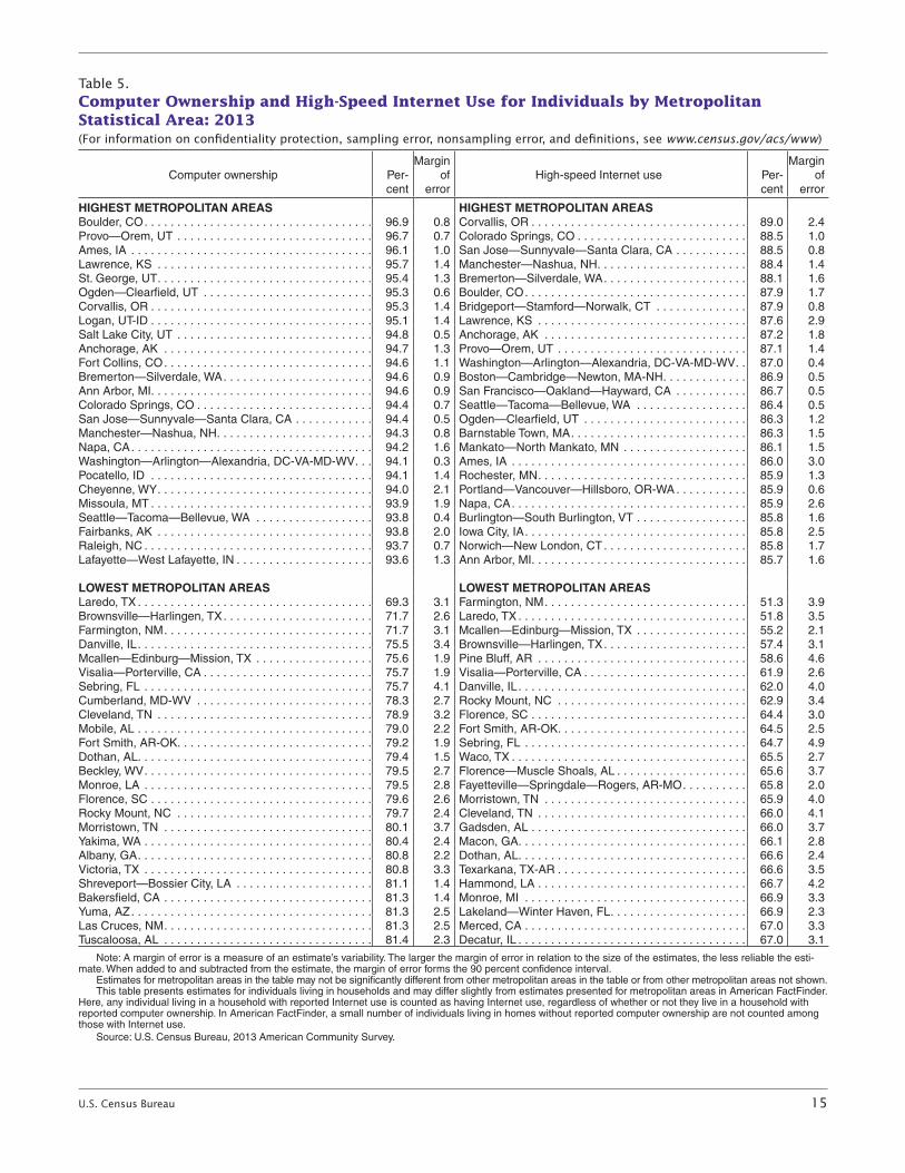
Table 5 provides estimates for individuals living in metropolitan areas with some of the highest and lowest rates of computer owner-ship and high-speed Internet use in the country. For computer owner-ship, metropolitan values ranged from 69.3 percent to 96.9 percent. On the lower end, only 3 metropoli-tan areas had rates of household computer ownership lower than 75 percent, 2 of them in Texas (Brownsville and Laredo), and 1 in New Mexico (Farmington). On the higher end, 3 metropolitan areas had household computer rates higher than 95 percent, including Boulder, Colorado; Provo, Utah; and Ames, Iowa.24

For high-speed Internet use, metropolitan values ranged from 51.3 percent to 89.0 percent. On the lower end, only 2 metropolitan areas had household high-speed Internet rates below 56.0 percent, including Farmington, New Mexico, and Laredo, Texas.25 On the higher end, only 4 areas had rates of household computer ownership significantly higher than 87.0 per-cent, including Colorado Springs, Colorado; San Jose, California; Manchester, New Hampshire; and Bridgeport, Connecticut.26

For computer and Internet use values for every metropolitan area in the United States, see Appendix Table D at <www.census.gov/hhes /computer/>.

24 Other metropolitan areas with point estimates higher than 95.0 were nevertheless not statistically different from 95 percent.

25 Despite having a point estimate below 56.0, the high-speed Internet rate for McAllen, TX, was not statistically different from 56 percent.

26 Other metropolitan areas had point esti-mates higher than 87.0 that were, neverthe-less, not statistically different from 87 percent.

U.S. C

ensu

s Bureau

1

3

RI

DE

MA

MD

NJ

CT

NHVT

WV

ME

SC

OH

KYVA

TN

MI

MS

IN

NY

LA

NC

PA

AR

ALGA

WI

MO

WA

OK

FL

ND

IA

MN

IL

NE

WY

SD

UT

KS

OR

CO

NM

ID

NV

AZ

MT

CA

TX

DC

AK

HI


0 500 Miles

0 100 Miles

0 100 Miles

Note: Metropolitan Statistical Areas defined by the Office of Management and Budget as of February 2013.

Figure 6.Computer Ownership for Individuals by Metropolitan Statistical Area: 2013

Percent ownershipcompared to thenational value

Higher by lessthan 5 percent

No statisticallysignificant difference

Lower by lessthan 5 percent

Higher by 5percent or more

Lower by 5 percent or more

U.S. percent is 88.4

14

U

.S. Cen

sus Bu

reau

RI

DE

MA

MD

NJ

CT

NHVT

WV

ME

SC

OH

KYVA

TN

MI

MS

IN

NY

LA

NC

PA

AR

ALGA

WI

MO

WA

OK

FL

ND

IA

MN

IL

NE

WY

SD

UT

KS

OR

CO

NM

ID

NV

AZ

MT

CA

TX

DC

AK

HI


0 500 Miles

0 100 Miles

0 100 Miles

Note: Metropolitan Statistical Areas defined by the Office of Management and Budget as of February 2013.

Figure 7.High-Speed Internet Use for Individuals by Metropolitan Statistical Area: 2013

Percent usagecompared to thenational value

Higher by lessthan 5 percent

No statisticallysignificant difference

Lower by lessthan 5 percent

Higher by 5percent or more

Lower by 5 percent or more

U.S. percent is 78.1


Table 5.Computer Ownership and High-Speed Internet Use for Individuals by Metropolitan Statistical Area: 2013(For information on confidentiality protection, sampling error, nonsampling error, and definitions, see www.census.gov/acs/www)

Computer ownership Per-cent

Margin of

errorHigh-speed Internet use Per-

cent

Margin of

error

HIGHEST METROPOLITAN AREAS HIGHEST METROPOLITAN AREASBoulder, CO . . . . . . . . . . . . . . . . . . . . . . . . . . . . . . . . . . . 96 .9 0 .8 Corvallis, OR . . . . . . . . . . . . . . . . . . . . . . . . . . . . . . . . . 89 .0 2 .4Provo—Orem, UT . . . . . . . . . . . . . . . . . . . . . . . . . . . . . . 96 .7 0 .7 Colorado Springs, CO . . . . . . . . . . . . . . . . . . . . . . . . . . 88 .5 1 .0Ames, IA . . . . . . . . . . . . . . . . . . . . . . . . . . . . . . . . . . . . . 96 .1 1 .0 San Jose—Sunnyvale—Santa Clara, CA . . . . . . . . . . . 88 .5 0 .8Lawrence, KS . . . . . . . . . . . . . . . . . . . . . . . . . . . . . . . . . 95 .7 1 .4 Manchester—Nashua, NH . . . . . . . . . . . . . . . . . . . . . . . 88 .4 1 .4St . George, UT . . . . . . . . . . . . . . . . . . . . . . . . . . . . . . . . . 95 .4 1 .3 Bremerton—Silverdale, WA . . . . . . . . . . . . . . . . . . . . . . 88 .1 1 .6Ogden—Clearfield, UT . . . . . . . . . . . . . . . . . . . . . . . . . . 95 .3 0 .6 Boulder, CO . . . . . . . . . . . . . . . . . . . . . . . . . . . . . . . . . . 87 .9 1 .7Corvallis, OR . . . . . . . . . . . . . . . . . . . . . . . . . . . . . . . . . . 95 .3 1 .4 Bridgeport—Stamford—Norwalk, CT . . . . . . . . . . . . . . 87 .9 0 .8Logan, UT-ID . . . . . . . . . . . . . . . . . . . . . . . . . . . . . . . . . . 95 .1 1 .4 Lawrence, KS . . . . . . . . . . . . . . . . . . . . . . . . . . . . . . . . 87 .6 2 .9Salt Lake City, UT . . . . . . . . . . . . . . . . . . . . . . . . . . . . . . 94 .8 0 .5 Anchorage, AK . . . . . . . . . . . . . . . . . . . . . . . . . . . . . . . 87 .2 1 .8Anchorage, AK . . . . . . . . . . . . . . . . . . . . . . . . . . . . . . . . 94 .7 1 .3 Provo—Orem, UT . . . . . . . . . . . . . . . . . . . . . . . . . . . . . 87 .1 1 .4Fort Collins, CO . . . . . . . . . . . . . . . . . . . . . . . . . . . . . . . . 94 .6 1 .1 Washington—Arlington—Alexandria, DC-VA-MD-WV . . 87 .0 0 .4Bremerton—Silverdale, WA . . . . . . . . . . . . . . . . . . . . . . . 94 .6 0 .9 Boston—Cambridge—Newton, MA-NH . . . . . . . . . . . . . 86 .9 0 .5Ann Arbor, MI . . . . . . . . . . . . . . . . . . . . . . . . . . . . . . . . . . 94 .6 0 .9 San Francisco—Oakland—Hayward, CA . . . . . . . . . . . 86 .7 0 .5Colorado Springs, CO . . . . . . . . . . . . . . . . . . . . . . . . . . . 94 .4 0 .7 Seattle—Tacoma—Bellevue, WA . . . . . . . . . . . . . . . . . 86 .4 0 .5San Jose—Sunnyvale—Santa Clara, CA . . . . . . . . . . . . 94 .4 0 .5 Ogden—Clearfield, UT . . . . . . . . . . . . . . . . . . . . . . . . . 86 .3 1 .2Manchester—Nashua, NH . . . . . . . . . . . . . . . . . . . . . . . . 94 .3 0 .8 Barnstable Town, MA . . . . . . . . . . . . . . . . . . . . . . . . . . . 86 .3 1 .5Napa, CA . . . . . . . . . . . . . . . . . . . . . . . . . . . . . . . . . . . . . 94 .2 1 .6 Mankato—North Mankato, MN . . . . . . . . . . . . . . . . . . . 86 .1 1 .5Washington—Arlington—Alexandria, DC-VA-MD-WV . . . 94 .1 0 .3 Ames, IA . . . . . . . . . . . . . . . . . . . . . . . . . . . . . . . . . . . . 86 .0 3 .0Pocatello, ID . . . . . . . . . . . . . . . . . . . . . . . . . . . . . . . . . . 94 .1 1 .4 Rochester, MN . . . . . . . . . . . . . . . . . . . . . . . . . . . . . . . . 85 .9 1 .3Cheyenne, WY . . . . . . . . . . . . . . . . . . . . . . . . . . . . . . . . . 94 .0 2 .1 Portland—Vancouver—Hillsboro, OR-WA . . . . . . . . . . . 85 .9 0 .6Missoula, MT . . . . . . . . . . . . . . . . . . . . . . . . . . . . . . . . . . 93 .9 1 .9 Napa, CA . . . . . . . . . . . . . . . . . . . . . . . . . . . . . . . . . . . . 85 .9 2 .6Seattle—Tacoma—Bellevue, WA . . . . . . . . . . . . . . . . . . 93 .8 0 .4 Burlington—South Burlington, VT . . . . . . . . . . . . . . . . . 85 .8 1 .6Fairbanks, AK . . . . . . . . . . . . . . . . . . . . . . . . . . . . . . . . . 93 .8 2 .0 Iowa City, IA . . . . . . . . . . . . . . . . . . . . . . . . . . . . . . . . . . 85 .8 2 .5Raleigh, NC . . . . . . . . . . . . . . . . . . . . . . . . . . . . . . . . . . . 93 .7 0 .7 Norwich—New London, CT . . . . . . . . . . . . . . . . . . . . . . 85 .8 1 .7Lafayette—West Lafayette, IN . . . . . . . . . . . . . . . . . . . . . 93 .6 1 .3 Ann Arbor, MI . . . . . . . . . . . . . . . . . . . . . . . . . . . . . . . . . 85 .7 1 .6

LOWEST METROPOLITAN AREAS LOWEST METROPOLITAN AREASLaredo, TX . . . . . . . . . . . . . . . . . . . . . . . . . . . . . . . . . . . . 69 .3 3 .1 Farmington, NM . . . . . . . . . . . . . . . . . . . . . . . . . . . . . . . 51 .3 3 .9Brownsville—Harlingen, TX . . . . . . . . . . . . . . . . . . . . . . . 71 .7 2 .6 Laredo, TX . . . . . . . . . . . . . . . . . . . . . . . . . . . . . . . . . . . 51 .8 3 .5Farmington, NM . . . . . . . . . . . . . . . . . . . . . . . . . . . . . . . . 71 .7 3 .1 Mcallen—Edinburg—Mission, TX . . . . . . . . . . . . . . . . . 55 .2 2 .1Danville, IL . . . . . . . . . . . . . . . . . . . . . . . . . . . . . . . . . . . . 75 .5 3 .4 Brownsville—Harlingen, TX . . . . . . . . . . . . . . . . . . . . . . 57 .4 3 .1Mcallen—Edinburg—Mission, TX . . . . . . . . . . . . . . . . . . 75 .6 1 .9 Pine Bluff, AR . . . . . . . . . . . . . . . . . . . . . . . . . . . . . . . . 58 .6 4 .6Visalia—Porterville, CA . . . . . . . . . . . . . . . . . . . . . . . . . . 75 .7 1 .9 Visalia—Porterville, CA . . . . . . . . . . . . . . . . . . . . . . . . . 61 .9 2 .6Sebring, FL . . . . . . . . . . . . . . . . . . . . . . . . . . . . . . . . . . . 75 .7 4 .1 Danville, IL . . . . . . . . . . . . . . . . . . . . . . . . . . . . . . . . . . . 62 .0 4 .0Cumberland, MD-WV . . . . . . . . . . . . . . . . . . . . . . . . . . . 78 .3 2 .7 Rocky Mount, NC . . . . . . . . . . . . . . . . . . . . . . . . . . . . . 62 .9 3 .4Cleveland, TN . . . . . . . . . . . . . . . . . . . . . . . . . . . . . . . . . 78 .9 3 .2 Florence, SC . . . . . . . . . . . . . . . . . . . . . . . . . . . . . . . . . 64 .4 3 .0Mobile, AL . . . . . . . . . . . . . . . . . . . . . . . . . . . . . . . . . . . . 79 .0 2 .2 Fort Smith, AR-OK . . . . . . . . . . . . . . . . . . . . . . . . . . . . . 64 .5 2 .5Fort Smith, AR-OK . . . . . . . . . . . . . . . . . . . . . . . . . . . . . . 79 .2 1 .9 Sebring, FL . . . . . . . . . . . . . . . . . . . . . . . . . . . . . . . . . . 64 .7 4 .9Dothan, AL . . . . . . . . . . . . . . . . . . . . . . . . . . . . . . . . . . . . 79 .4 1 .5 Waco, TX . . . . . . . . . . . . . . . . . . . . . . . . . . . . . . . . . . . . 65 .5 2 .7Beckley, WV . . . . . . . . . . . . . . . . . . . . . . . . . . . . . . . . . . . 79 .5 2 .7 Florence—Muscle Shoals, AL . . . . . . . . . . . . . . . . . . . . 65 .6 3 .7Monroe, LA . . . . . . . . . . . . . . . . . . . . . . . . . . . . . . . . . . . 79 .5 2 .8 Fayetteville—Springdale—Rogers, AR-MO . . . . . . . . . . 65 .8 2 .0Florence, SC . . . . . . . . . . . . . . . . . . . . . . . . . . . . . . . . . . 79 .6 2 .6 Morristown, TN . . . . . . . . . . . . . . . . . . . . . . . . . . . . . . . 65 .9 4 .0Rocky Mount, NC . . . . . . . . . . . . . . . . . . . . . . . . . . . . . . 79 .7 2 .4 Cleveland, TN . . . . . . . . . . . . . . . . . . . . . . . . . . . . . . . . 66 .0 4 .1Morristown, TN . . . . . . . . . . . . . . . . . . . . . . . . . . . . . . . . 80 .1 3 .7 Gadsden, AL . . . . . . . . . . . . . . . . . . . . . . . . . . . . . . . . . 66 .0 3 .7Yakima, WA . . . . . . . . . . . . . . . . . . . . . . . . . . . . . . . . . . . 80 .4 2 .4 Macon, GA . . . . . . . . . . . . . . . . . . . . . . . . . . . . . . . . . . . 66 .1 2 .8Albany, GA . . . . . . . . . . . . . . . . . . . . . . . . . . . . . . . . . . . . 80 .8 2 .2 Dothan, AL . . . . . . . . . . . . . . . . . . . . . . . . . . . . . . . . . . . 66 .6 2 .4Victoria, TX . . . . . . . . . . . . . . . . . . . . . . . . . . . . . . . . . . . 80 .8 3 .3 Texarkana, TX-AR . . . . . . . . . . . . . . . . . . . . . . . . . . . . . 66 .6 3 .5Shreveport—Bossier City, LA . . . . . . . . . . . . . . . . . . . . . 81 .1 1 .4 Hammond, LA . . . . . . . . . . . . . . . . . . . . . . . . . . . . . . . . 66 .7 4 .2Bakersfield, CA . . . . . . . . . . . . . . . . . . . . . . . . . . . . . . . . 81 .3 1 .4 Monroe, MI . . . . . . . . . . . . . . . . . . . . . . . . . . . . . . . . . . 66 .9 3 .3Yuma, AZ . . . . . . . . . . . . . . . . . . . . . . . . . . . . . . . . . . . . . 81 .3 2 .5 Lakeland—Winter Haven, FL . . . . . . . . . . . . . . . . . . . . . 66 .9 2 .3Las Cruces, NM . . . . . . . . . . . . . . . . . . . . . . . . . . . . . . . . 81 .3 2 .5 Merced, CA . . . . . . . . . . . . . . . . . . . . . . . . . . . . . . . . . . 67 .0 3 .3Tuscaloosa, AL . . . . . . . . . . . . . . . . . . . . . . . . . . . . . . . . 81 .4 2 .3 Decatur, IL . . . . . . . . . . . . . . . . . . . . . . . . . . . . . . . . . . . 67 .0 3 .1

Note: A margin of error is a measure of an estimate’s variability . The larger the margin of error in relation to the size of the estimates, the less reliable the esti-mate . When added to and subtracted from the estimate, the margin of error forms the 90 percent confidence interval .

Estimates for metropolitan areas in the table may not be significantly different from other metropolitan areas in the table or from other metropolitan areas not shown .This table presents estimates for individuals living in households and may differ slightly from estimates presented for metropolitan areas in American FactFinder .

Here, any individual living in a household with reported Internet use is counted as having Internet use, regardless of whether or not they live in a household with reported computer ownership . In American FactFinder, a small number of individuals living in homes without reported computer ownership are not counted among those with Internet use .



SOURCE OF THE DATA

The data used in this report comes from the ACS, a large and continu-ous national level data collection effort performed by the Census Bureau. Designed to replace the once-a-decade long-form data col-lected with the Decennial Census, the ACS program routinely provides ongoing data and updated infor-mation for all parts of the coun-try. Each month, about 290,000 households are asked to complete a questionnaire, followed by tele-phone and person-visit interviews for nonresponding households.27

The program uses a design that accumulates data over increasingly longer periods of time, in order to provide data products for increas-ingly smaller geographic units. The first level of collection aggregation occurs over a single year, produces a data set of about 3.5 million households, and provides estimates for all geographic units with 65,000 people or more. This report relies on this single-year data.

Other levels of aggregation include “3-year” data sets, which pool 3 separate years of data together to provide estimates for geographies with 20,000 people or more, and “5-year” data sets, which pool 4 separate years of data together to provide estimates for geographies down to the block group level—or areas as small as several thousand households. These ACS multiyear products are now fully operational, meaning that when new single-year data are collected, they are imme-diately incorporated to provide updated 3-year and 5-year data for all parts of the country. However,

27 Although the ACS sample includes peo-ple living in households, and was expanded in 2006 to include people living in group quarters (i.e., nursing homes, correctional facilities, military barracks, and college/univer-sity housing), computer and Internet questions were not collected for group quarters. For more general information on the ACS, please visit <www.census.gov/acs/www/>.

because 2013 is the first year the ACS included computer and Internet questions, the first “3-year” estimates on this topic will be avail-able for the year 2015, and the first “5-year” estimates will be available for 2017.

The estimates in this report come from data obtained in the 2013 ACS. The population represented (the population universe) in the ACS includes all people living in households, plus individuals living in group quarters. Because the computer and Internet variables used to create this report were not asked in group quarters, this report excludes all of those individuals from the analysis.

COMPARISON WITH OTHER DATA SOURCES

As discussed at the beginning of this report, the Census Bureau has historically collected computer and Internet data via the CPS. Due to differences in data collection, users should be cautious about directly comparing estimates from these two separate data sources. Previous census releases can be found at <www.census.gov/hhes /computer/>.

ACCURACY OF THE ESTIMATES

Statistics from surveys are subject to sampling and nonsampling error. All comparisons presented in this report have taken sampling error into account.

Sampling error is the difference between an estimate based on a sample and a corresponding value that would be obtained if the estimate were based on the entire population (as from a census). Measures of the sampling error are provided in the form of margins of error for all estimates included in this report. All comparative state-ments have undergone statistical

testing, and comparisons are significant at the 90 percent level unless otherwise noted. In addition, nonsampling error may be intro-duced during any of the operations used to collect and process survey data. To minimize these errors, the Census Bureau employs qual-ity control procedures in sample selection, the wording of questions, interviewing, coding, data process-ing, and data analysis.

For more information on sampling and estimation methods, confiden-tiality protection, and sampling and nonsampling errors, please see the 2013 ACS Accuracy of the Data document located at <www.census.gov/acs/www /data_documentation /documentation_main/>.

USER CONTACTS

The Census Bureau welcomes the comments and advice of users of its data and reports. If you have any suggestions or comments, contact:

Thom File <[email protected]>

or

Camille Ryan <[email protected]>.

Alternatively, you can write to:

Chief, SEHSD Division U.S. Census Bureau Washington, DC 20233-8800

or send an e-mail to <[email protected]>.

SUGGESTED CITATION

File, Thom and Camille Ryan, “Computer and Internet Use in the United States: 2013,” American Community Survey Reports, ACS-28, U.S. Census Bureau, Washington, DC, 2014.

computer and internet use in the united states: 2013 · access to broadband technologies, ......

Documents