computer aided engineering applications 3. advanced...
TRANSCRIPT
Computer Aided Engineering
Applications
3. Advanced Manufacturing 3.1 CAM systems
3.2 Geometry of surfaces
Engi 6928 - Fall 2014
3.2 Geometry of surfaces
3.3 Product data exchange
3.4 Data Communication
3.5 Automated Manufacturing systems
3.6 Part programming
3.1 CAM systems3.1 CAM systems
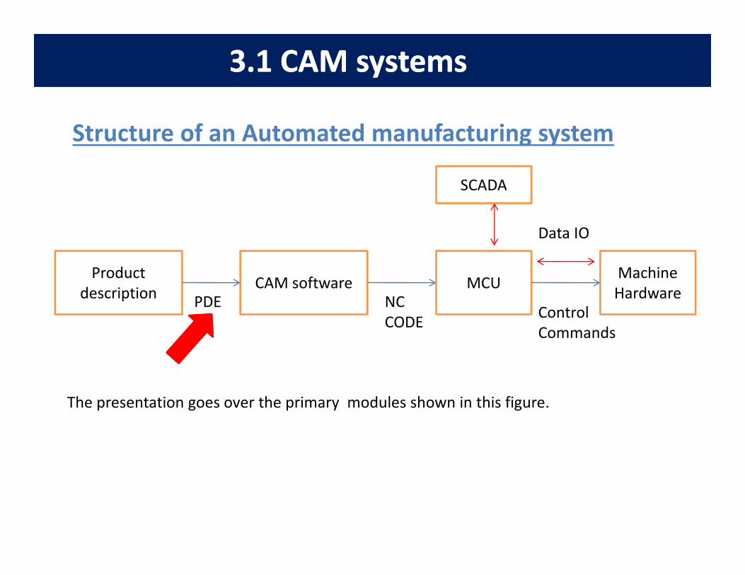
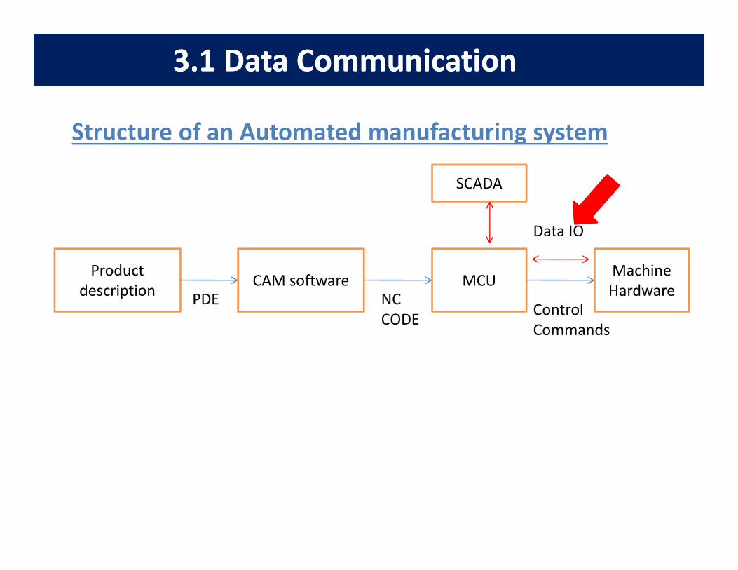
Structure of an Automated manufacturing system
Product
descriptionCAM software MCU
Machine
Hardware
Data IO
SCADA
descriptionCAM software MCU
HardwarePDE NC
CODEControl
Commands
The presentation goes over the primary modules shown in this figure.
3.2 Geometry of curves and surfaces3.2 Geometry of curves and surfaces
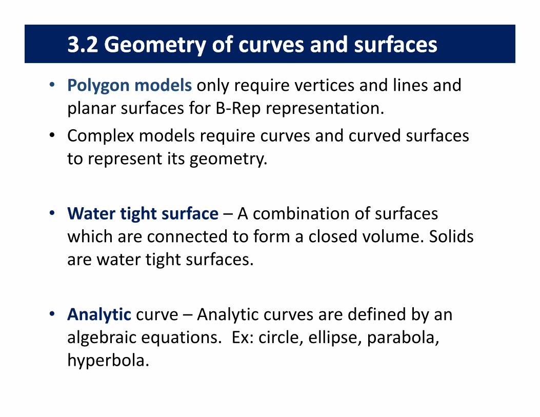
• Polygon models only require vertices and lines and
planar surfaces for B-Rep representation.
• Complex models require curves and curved surfaces
to represent its geometry.
• Water tight surface – A combination of surfaces • Water tight surface – A combination of surfaces
which are connected to form a closed volume. Solids
are water tight surfaces.
• Analytic curve – Analytic curves are defined by an
algebraic equations. Ex: circle, ellipse, parabola,
hyperbola.
3.2 Geometry of curves and surfaces3.2 Geometry of curves and surfaces
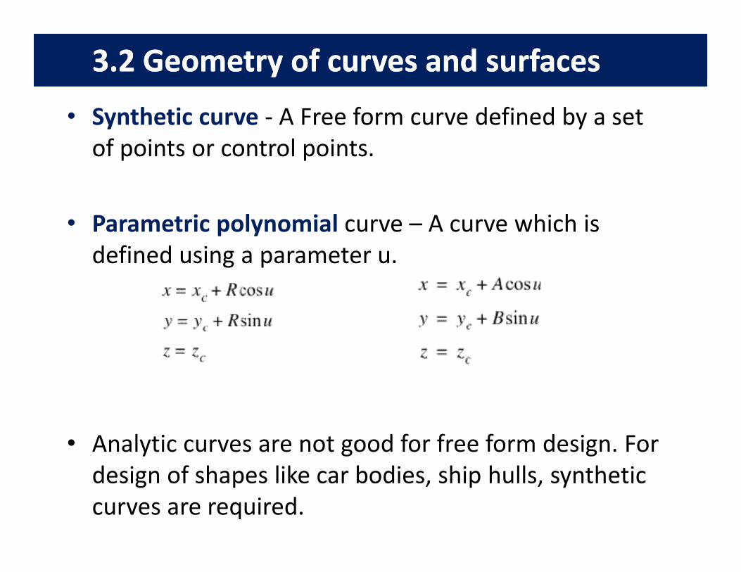
• Synthetic curve - A Free form curve defined by a set
of points or control points.
• Parametric polynomial curve – A curve which is
defined using a parameter u.
• Analytic curves are not good for free form design. For
design of shapes like car bodies, ship hulls, synthetic
curves are required.
3.2 Geometry of curves and surfaces3.2 Geometry of curves and surfaces
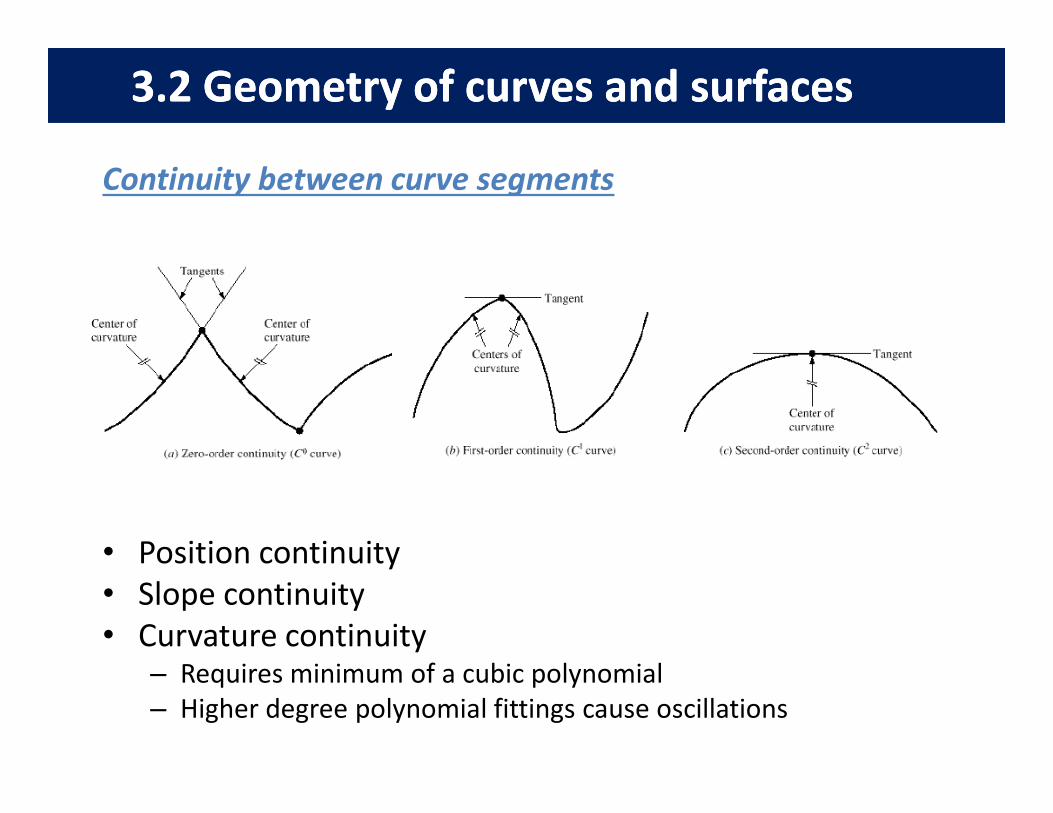
Continuity between curve segments
• Position continuity
• Slope continuity
• Curvature continuity– Requires minimum of a cubic polynomial
– Higher degree polynomial fittings cause oscillations
3.2 Geometry of curves and surfaces3.2 Geometry of curves and surfaces
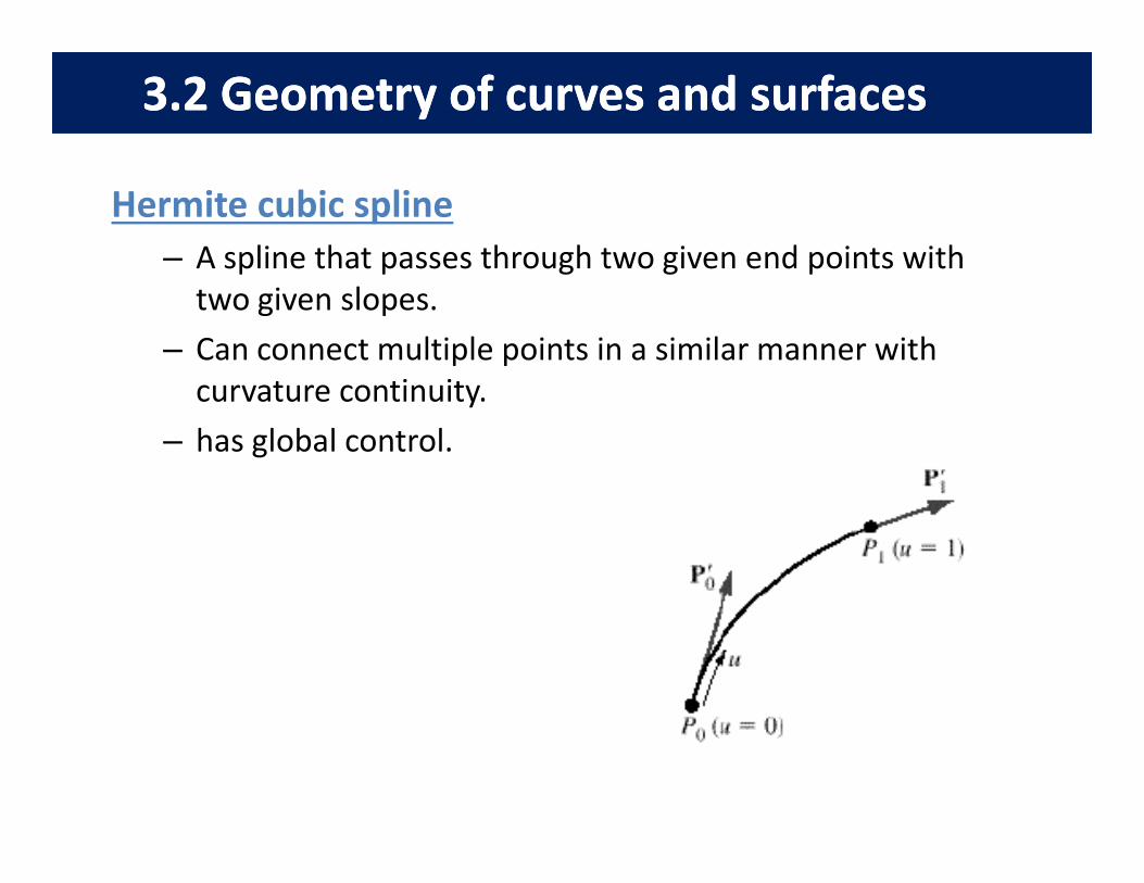
Hermite cubic spline
– A spline that passes through two given end points with
two given slopes.
– Can connect multiple points in a similar manner with
curvature continuity.
– has global control.– has global control.
3.2 Geometry of curves and surfaces3.2 Geometry of curves and surfaces
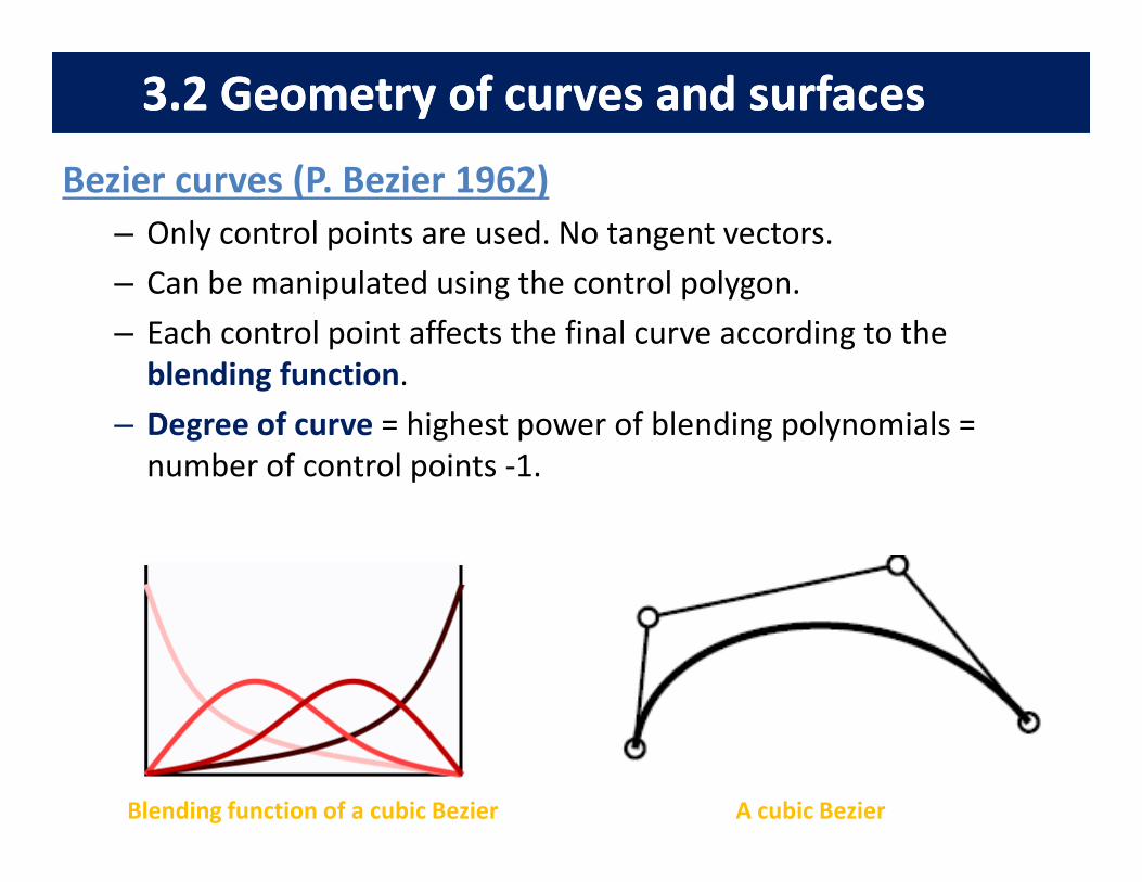
Bezier curves (P. Bezier 1962)
– Only control points are used. No tangent vectors.
– Can be manipulated using the control polygon.
– Each control point affects the final curve according to the
blending function.
– Degree of curve = highest power of blending polynomials = – Degree of curve = highest power of blending polynomials =
number of control points -1.
Blending function of a cubic Bezier A cubic Bezier
3.2 Geometry of curves and surfaces3.2 Geometry of curves and surfaces
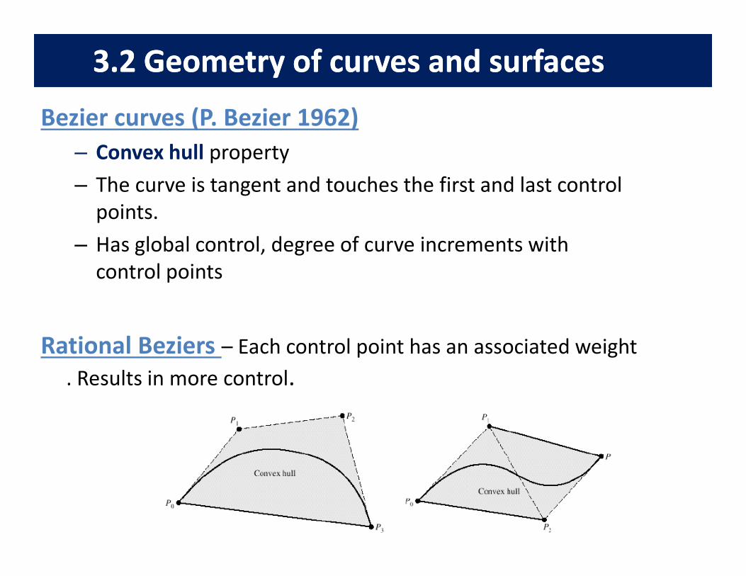
Bezier curves (P. Bezier 1962)
– Convex hull property
– The curve is tangent and touches the first and last control
points.
– Has global control, degree of curve increments with
control points
Rational Beziers – Each control point has an associated weight
. Results in more control.
3.2 Geometry of curves and surfaces3.2 Geometry of curves and surfaces
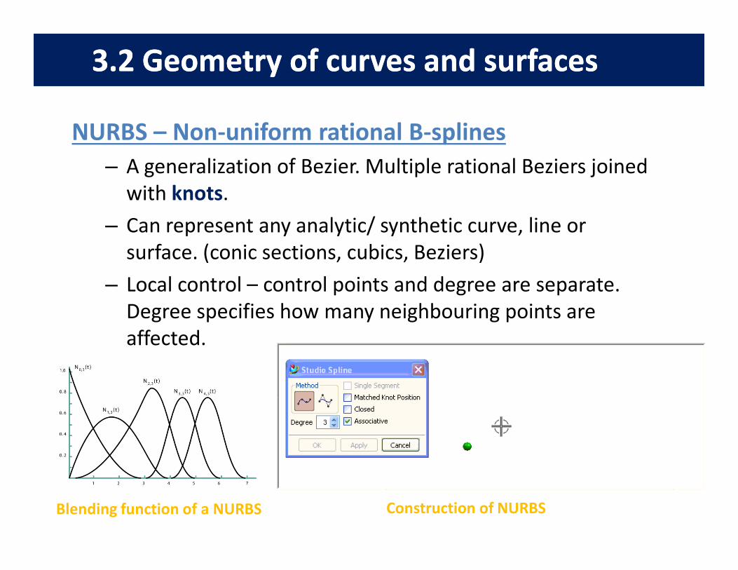
NURBS – Non-uniform rational B-splines
– A generalization of Bezier. Multiple rational Beziers joined
with knots.
– Can represent any analytic/ synthetic curve, line or
surface. (conic sections, cubics, Beziers)
– Local control – control points and degree are separate. – Local control – control points and degree are separate.
Degree specifies how many neighbouring points are
affected.
Blending function of a NURBS Construction of NURBS
"
3.2 Geometry of curves and surfaces3.2 Geometry of curves and surfaces
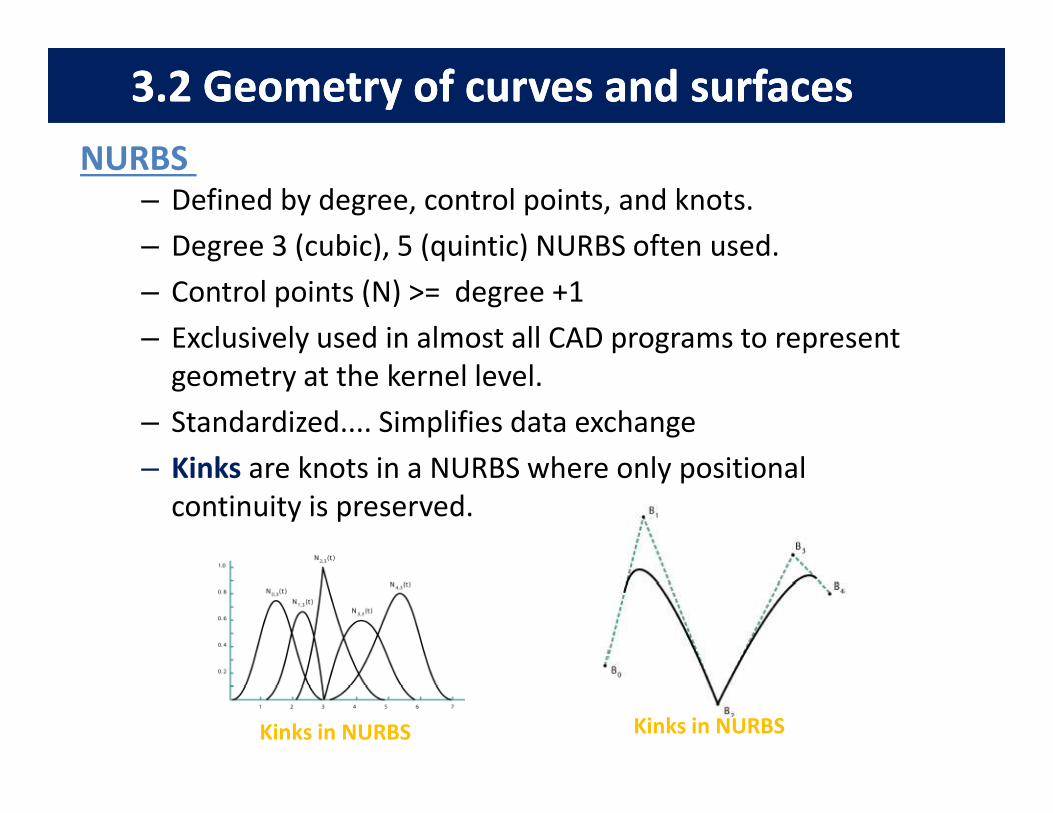
– Defined by degree, control points, and knots.
– Degree 3 (cubic), 5 (quintic) NURBS often used.
– Control points (N) >= degree +1
– Exclusively used in almost all CAD programs to represent
geometry at the kernel level.
– Standardized.... Simplifies data exchange
NURBS
– Standardized.... Simplifies data exchange
– Kinks are knots in a NURBS where only positional
continuity is preserved.
Kinks in NURBSKinks in NURBS
3.2 Geometry of curves and surfaces3.2 Geometry of curves and surfaces
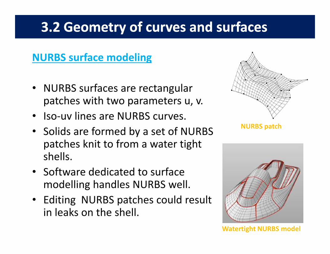
NURBS surface modeling
• NURBS surfaces are rectangular patches with two parameters u, v.
• Iso-uv lines are NURBS curves.
• Solids are formed by a set of NURBS NURBS patch
• Solids are formed by a set of NURBS patches knit to from a water tight shells.
• Software dedicated to surface modelling handles NURBS well.
• Editing NURBS patches could result in leaks on the shell.
NURBS patch
Watertight NURBS model
3.2 Geometry of curves and surfaces3.2 Geometry of curves and surfaces
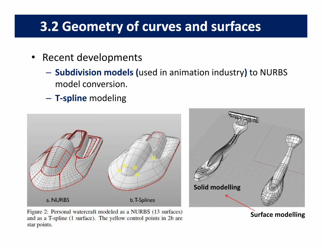
• Recent developments
– Subdivision models (used in animation industry) to NURBS
model conversion.
– T-spline modeling
Surface modelling
Solid modelling
3.2 Geometry of curves and surfaces3.2 Geometry of curves and surfaces
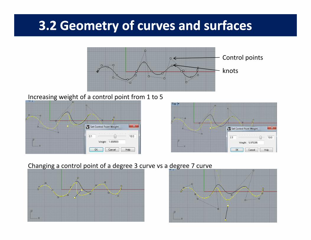
Control points
knots
Increasing weight of a control point from 1 to 5
Changing a control point of a degree 3 curve vs a degree 7 curve
3.3 Product data exchange3.3 Product data exchange
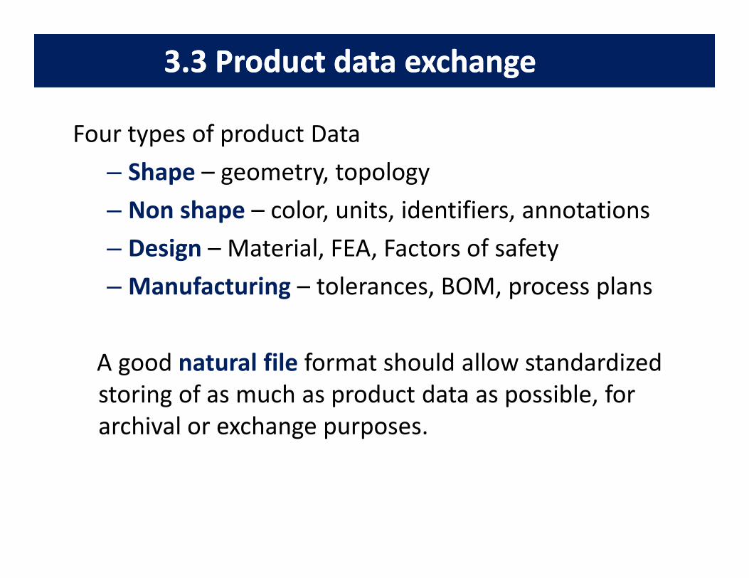
Four types of product Data
– Shape – geometry, topology
– Non shape – color, units, identifiers, annotations
– Design – Material, FEA, Factors of safety
– Manufacturing – tolerances, BOM, process plans– Manufacturing – tolerances, BOM, process plans
A good natural file format should allow standardized
storing of as much as product data as possible, for
archival or exchange purposes.
3.3 Product data exchange3.3 Product data exchange
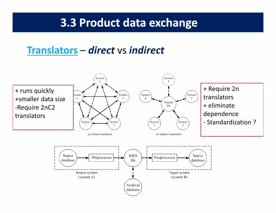
Translators – direct vs indirect
+ runs quickly
+smaller data size
-Require 2nC2
+ Require 2n
translators
+ eliminate -Require 2nC2
translators
+ eliminate
dependence
- Standardization ?
3.3 Product data exchange3.3 Product data exchange
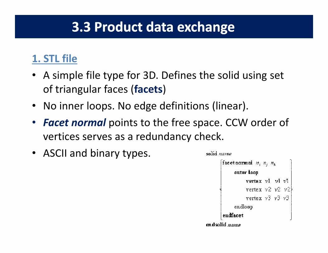
1. STL file
• A simple file type for 3D. Defines the solid using set
of triangular faces (facets)
• No inner loops. No edge definitions (linear).
• Facet normal points to the free space. CCW order of • Facet normal points to the free space. CCW order of
vertices serves as a redundancy check.
• ASCII and binary types.
3.3 Product data exchange3.3 Product data exchange
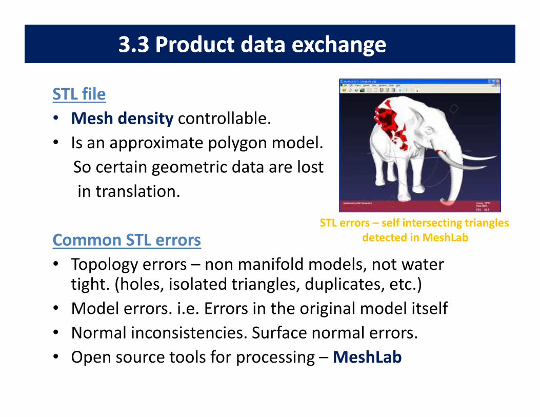
STL file
• Mesh density controllable.
• Is an approximate polygon model.
So certain geometric data are lost
in translation.
Common STL errors
• Topology errors – non manifold models, not water tight. (holes, isolated triangles, duplicates, etc.)
• Model errors. i.e. Errors in the original model itself
• Normal inconsistencies. Surface normal errors.
• Open source tools for processing – MeshLab
STL errors – self intersecting triangles
detected in MeshLab
3.3 Product data exchange3.3 Product data exchange
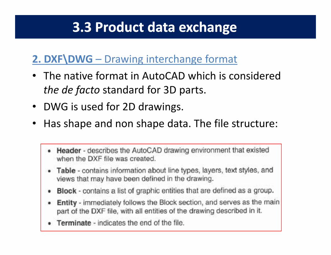
2. DXF\DWG – Drawing interchange format
• The native format in AutoCAD which is considered
the de facto standard for 3D parts.
• DWG is used for 2D drawings.
• Has shape and non shape data. The file structure:• Has shape and non shape data. The file structure:
3.3 Product data exchange3.3 Product data exchange
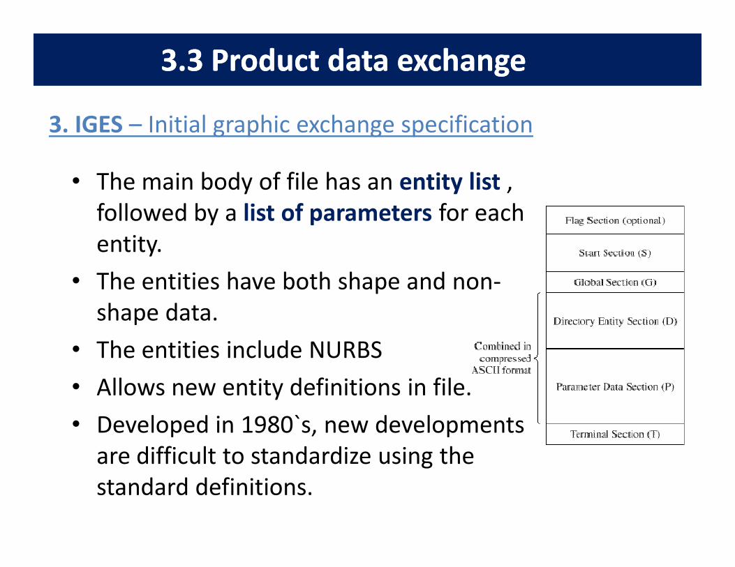
• The main body of file has an entity list ,
followed by a list of parameters for each
entity.
• The entities have both shape and non-
3. IGES – Initial graphic exchange specification
• The entities have both shape and non-
shape data.
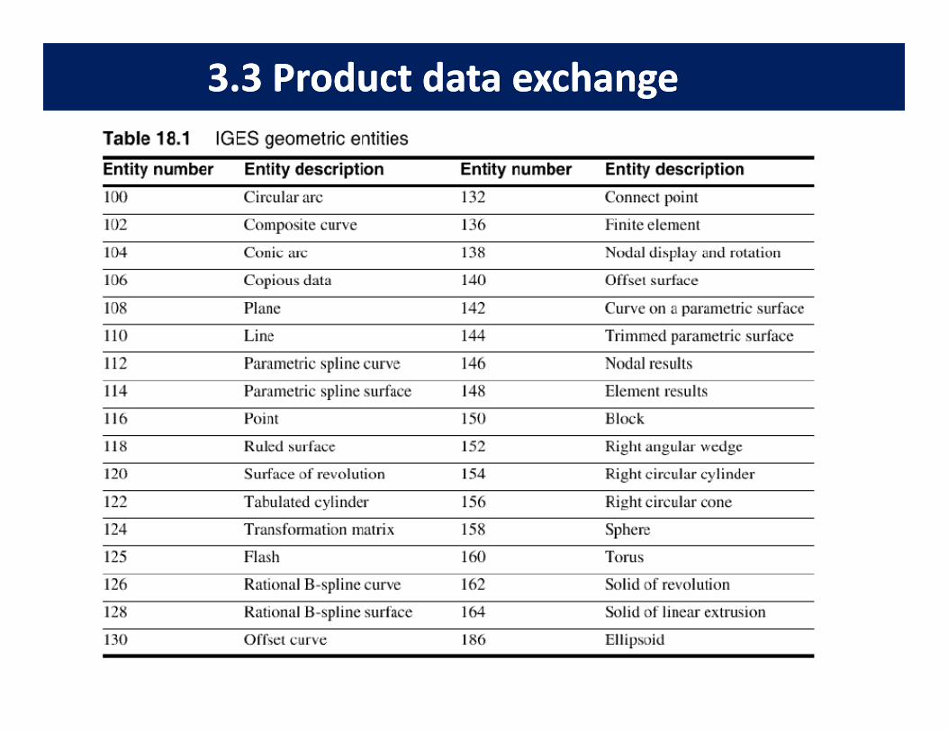
• The entities include NURBS
• Allows new entity definitions in file.
• Developed in 1980`s, new developments
are difficult to standardize using the
standard definitions.
3.3 Product data exchange3.3 Product data exchange
ᣠΆ
3.3 Product data exchange3.3 Product data exchange
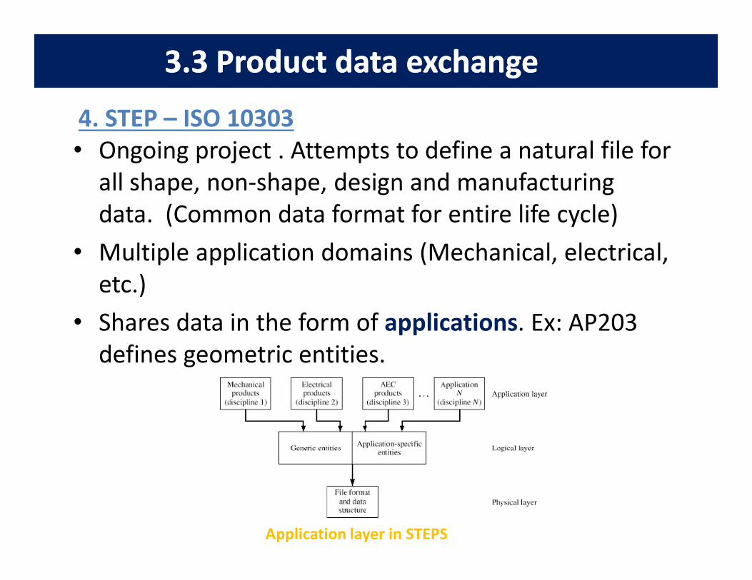
• Ongoing project . Attempts to define a natural file for
all shape, non-shape, design and manufacturing
data. (Common data format for entire life cycle)
• Multiple application domains (Mechanical, electrical,
etc.)
4. STEP – ISO 10303
etc.)
• Shares data in the form of applications. Ex: AP203
defines geometric entities.
Application layer in STEPS
3.3 Product data exchange3.3 Product data exchange
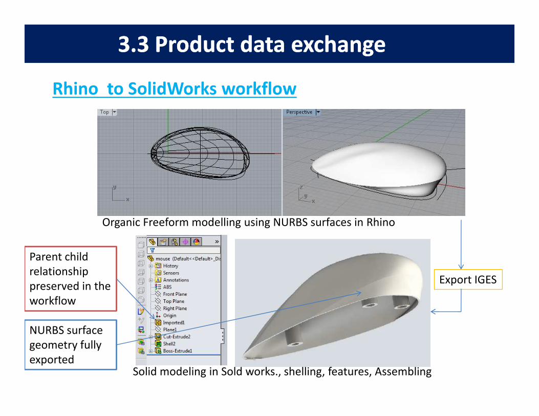
Rhino to SolidWorks workflow
Organic Freeform modelling using NURBS surfaces in Rhino
Solid modeling in Sold works., shelling, features, Assembling
Export IGES
Parent child
relationship
preserved in the
workflow
NURBS surface
geometry fully
exported
粠ҡ
3.1 Data Communication3.1 Data Communication
Structure of an Automated manufacturing system
Product
descriptionCAM software MCU
Machine
Hardware
Data IO
SCADA
descriptionCAM software MCU
HardwarePDE NC
CODEControl
Commands
3.4 Data Communication3.4 Data Communication
• Data communication is used to transfer data to and
from manufacturing machines.
• These data are essential for process control, where
the efficiency and quality of the production line is
tracked and corrected as necessary. Also required for
factory automation, remote monitoring etc..factory automation, remote monitoring etc..
• The data is often displayed on SCADA (Supervisory
control and Data Acquisition) units, which can be a
panel or a GUI interface in a PC.
肐ҡ
3.4 Data Communication3.4 Data Communication
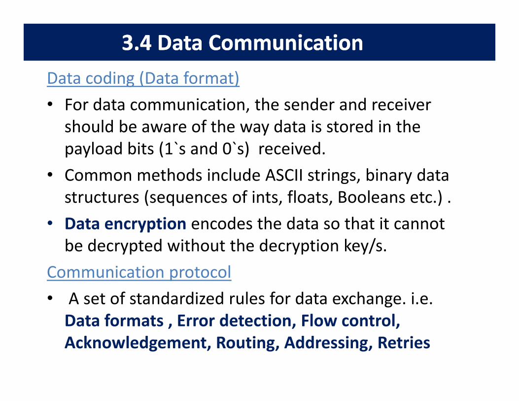
Data coding (Data format)
• For data communication, the sender and receiver
should be aware of the way data is stored in the
payload bits (1`s and 0`s) received.
• Common methods include ASCII strings, binary data
structures (sequences of ints, floats, Booleans etc.) .structures (sequences of ints, floats, Booleans etc.) .
• Data encryption encodes the data so that it cannot
be decrypted without the decryption key/s.
Communication protocol
• A set of standardized rules for data exchange. i.e.
Data formats , Error detection, Flow control,
Acknowledgement, Routing, Addressing, Retries
ᣠΆ
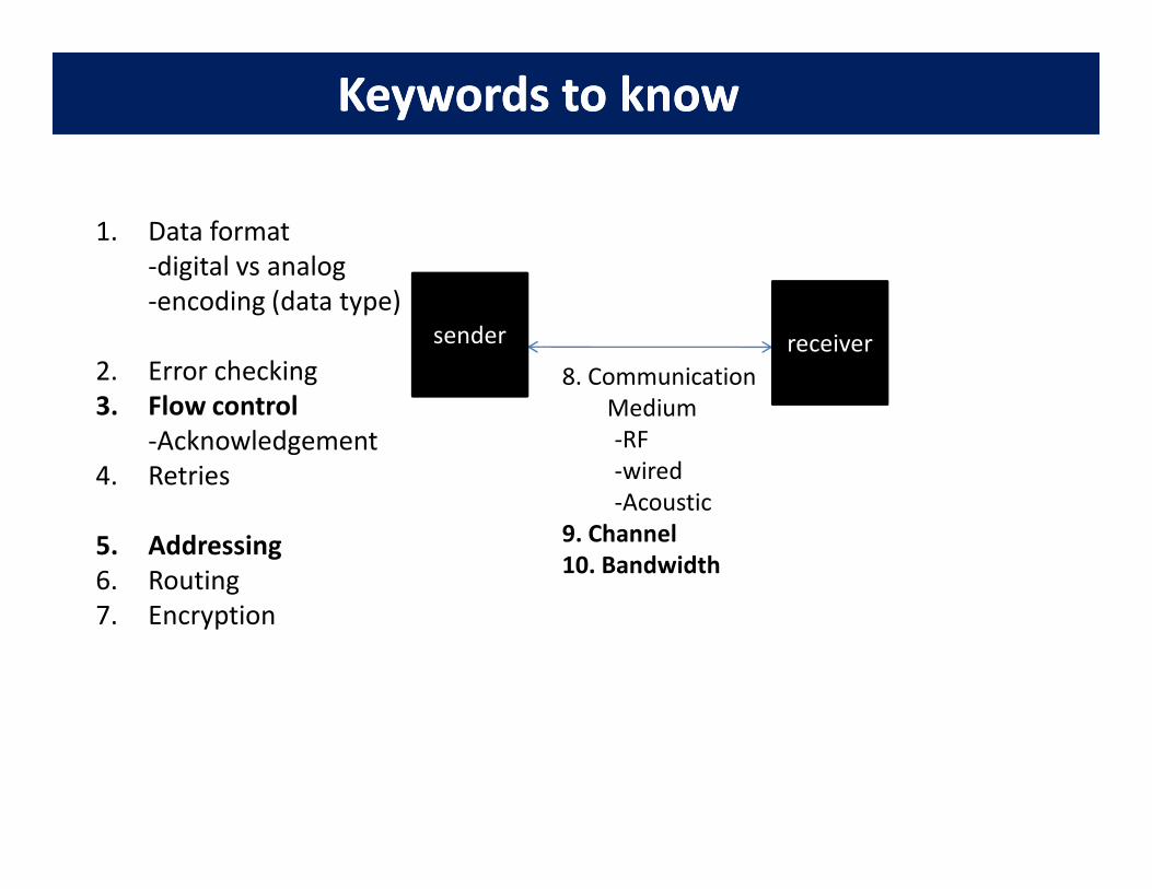
Keywords to knowKeywords to know
sender
8. Communication
Medium
-RF
1. Data format
-digital vs analog
-encoding (data type)
2. Error checking
3. Flow control
-Acknowledgement
receiver
-RF
-wired
-Acoustic
9. Channel
10. Bandwidth
-Acknowledgement
4. Retries
5. Addressing
6. Routing
7. Encryption
3.4 Data Communication3.4 Data Communication
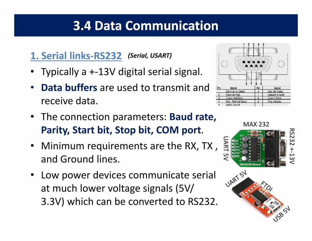
1. Serial links-RS232
• Typically a +-13V digital serial signal.
• Data buffers are used to transmit and
receive data.
• The connection parameters: Baud rate, MAX 232
(Serial, USART)
• The connection parameters: Baud rate,
Parity, Start bit, Stop bit, COM port.
• Minimum requirements are the RX, TX ,
and Ground lines.
• Low power devices communicate serial
at much lower voltage signals (5V/
3.3V) which can be converted to RS232.
RS
23
2 +
-13
V
UA
RT
5V
MAX 232
ᣠҩ
3.4 Data Communication3.4 Data Communication
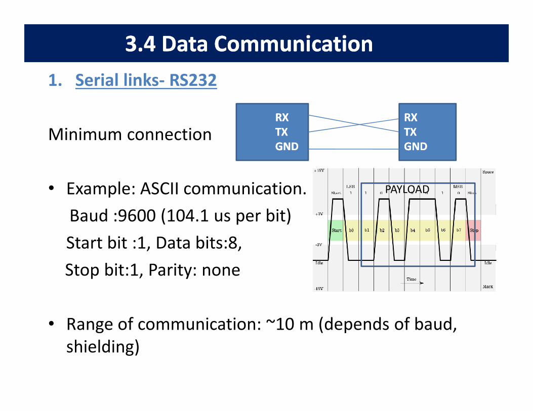
1. Serial links- RS232
Minimum connection
• Example: ASCII communication.
Baud :9600 (104.1 us per bit)
RXRX
TXTX
GNDGND
RXRX
TXTX
GNDGND
PAYLOAD
Baud :9600 (104.1 us per bit)
Start bit :1, Data bits:8,
Stop bit:1, Parity: none
• Range of communication: ~10 m (depends of baud,
shielding)
鎠ҥ
3.4 Data Communication3.4 Data Communication
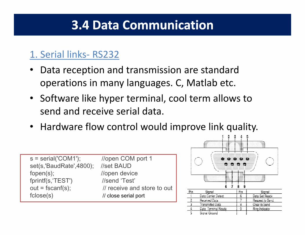
1. Serial links- RS232
• Data reception and transmission are standard
operations in many languages. C, Matlab etc.
• Software like hyper terminal, cool term allows to
send and receive serial data.
• Hardware flow control would improve link quality.
s = serial('COM1'); //open COM port 1set(s,'BaudRate',4800); //set BAUDfopen(s); //open devicefprintf(s,‘TEST') //send ‘Test’out = fscanf(s); // receive and store to outfclose(s) // close serial port
փ
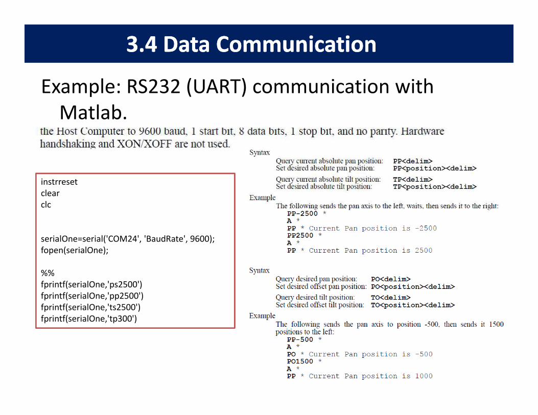
3.4 Data Communication3.4 Data Communication
Example: RS232 (UART) communication with
Matlab.
instrreset
clear
clcclc
serialOne=serial('COM24', 'BaudRate', 9600);
fopen(serialOne);
%%
fprintf(serialOne,'ps2500')
fprintf(serialOne,'pp2500')
fprintf(serialOne,'ts2500')
fprintf(serialOne,'tp300')
ᣠҧ
3.4 Data Communication3.4 Data Communication
2. Local Area Networks- LAN
• LAN is good for network of devices and allows much
higher data rates (100 Mbps)
• Confined to 10Km in distance.
• WLAN uses a wireless medium (2.4GHz RF). LAN • WLAN uses a wireless medium (2.4GHz RF). LAN
uses wired medium (twisted pair)
• LANs have well established protocols for networking,
traffic control, and error recovery.
• TCP/IP and UDP protocols are popular.
3.4 Data Communication3.4 Data Communication
2. LAN/ WLAN
• LAN communicates packets of Data.
• Each device in the network is assigned an IP address.
• Different Ports can be used under the same IP address so
that many application can access the LAN.
• Applications can run as a client (A requesting machine) • Applications can run as a client (A requesting machine)
or a server (a responding machine)
• The packet header contains the data of source and
destination , error checking info.
• Error checking is performed using check sum. (a number
representing the addition of all data bits in the payload)
ᣠҧ
3.4 Data Communication3.4 Data Communication
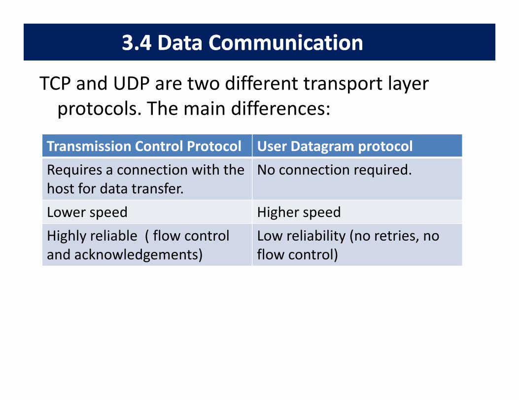
TCP and UDP are two different transport layer
protocols. The main differences:
Transmission Control Protocol User Datagram protocol
Requires a connection with the
host for data transfer.
No connection required.
Lower speed Higher speed
Highly reliable ( flow control
and acknowledgements)
Low reliability (no retries, no
flow control)
3.4 Data Communication3.4 Data Communication
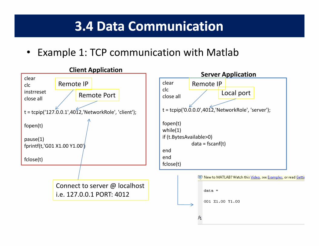
• Example 1: TCP communication with Matlab
clear
clc
instrreset
close all
t = tcpip(‘127.0.0.1',4012,'NetworkRole', 'client');
fopen(t)
clear
clc
close all
t = tcpip('0.0.0.0',4012,'NetworkRole', 'server');
fopen(t)
Client ApplicationServer Application
Remote IP
Remote Port
Remote IP
Local port
fopen(t)
pause(1)
fprintf(t,'G01 X1.00 Y1.00')
fclose(t)
fopen(t)
while(1)
if (t.BytesAvailable>0)
data = fscanf(t)
end
end
fclose(t)
Connect to server @ localhost
i.e. 127.0.0.1 PORT: 4012
ᣠҧ
3.4 Data Communication3.4 Data Communication
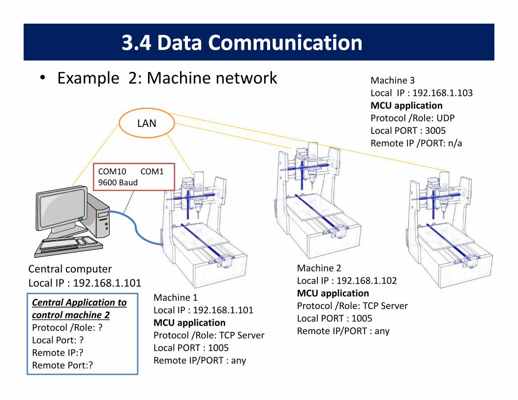
• Example 2: Machine network Machine 3
Local IP : 192.168.1.103
MCU application
Protocol /Role: UDP
Local PORT : 3005
Remote IP /PORT: n/a
LAN
COM10 COM1
9600 Baud
Machine 1
Local IP : 192.168.1.101
MCU application
Protocol /Role: TCP Server
Local PORT : 1005
Remote IP/PORT : any
Machine 2
Local IP : 192.168.1.102
MCU application
Protocol /Role: TCP Server
Local PORT : 1005
Remote IP/PORT : any
Central computer
Local IP : 192.168.1.101
Central Application to
control machine 2
Protocol /Role: ?
Local Port: ?
Remote IP:?
Remote Port:?
3.4 Data Communication3.4 Data Communication
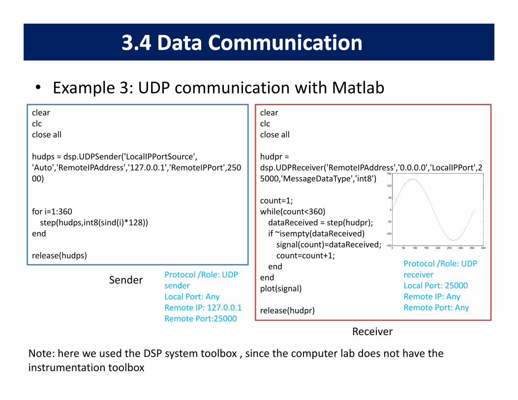
• Example 3: UDP communication with Matlab
clear
clc
close all
hudpr =
dsp.UDPReceiver('RemoteIPAddress','0.0.0.0','LocalIPPort',2
5000,'MessageDataType','int8')
count=1;
clear
clc
close all
hudps = dsp.UDPSender('LocalIPPortSource',
'Auto','RemoteIPAddress','127.0.0.1','RemoteIPPort',250
00)
50
100
150
count=1;
while(count<360)
dataReceived = step(hudpr);
if ~isempty(dataReceived)
signal(count)=dataReceived;
count=count+1;
end
end
plot(signal)
release(hudpr)
for i=1:360
step(hudps,int8(sind(i)*128))
end
release(hudps)
Sender
Receiver
0 50 100 150 200 250 300 350 400-150
-100
-50
0
Note: here we used the DSP system toolbox , since the computer lab does not have the
instrumentation toolbox
Protocol /Role: UDP
sender
Local Port: Any
Remote IP: 127.0.0.1
Remote Port:25000
Protocol /Role: UDP
receiver
Local Port: 25000
Remote IP: Any
Remote Port: Any