computer aided design of an injection molded center-gated disc

UNIVERSITY OF THESSALY

SCHOOL OF ENGINEERING

DEPARTMENT OF MECHANICAL ENGINEERING

PROGRAM OF POSTGRADUATE STUDIES

ΚΑΡΑΓΙΑΝΝΗΣ ΣΤΑΥΡΟΣ - ΘΕΟΔΩΡΟΣ

Computer Aided Design of an Injection Molded Center-Gated Disc

Greece, Volos, March 2014

Institutional Repository - Library & Information Centre - University of Thessaly09/12/2017 02:47:56 EET - 137.108.70.7

Division of Energy, Industrial Processes & Pollution Abatement

Technology

This thesis was approved by the Final Examination Committee:

First examiner: Papathanasiou Athanasios

(Advisor) Asssociate Professor, University of Thessaly, Department of

Mechanical Engineering

Second examiner: Bontozoglou Vasilis

Professor, University of Thessaly, Department of Mechanical

Engineering

Third examiner: Andritsos Nikos

Professor, University of Thessaly, Department of Mechanical

Engineering

Academic year 2013-2014

3rd

Semester (Fall)


CONTENTS

1. Introduction

1.1 Structure of polymers ..................................................................................................... 1

1.2 Thermoplastics classification based on morphology ..................................................... 2

1.3 Basics of injection molding ........................................................................................... 3

1.4 Polymer flow behavior in injection molding ............................................................... 12

1.4.1 How plastic fills a mold ...................................................................................... 12

1.4.2 Cross-sectional flow and molecular orientation ................................................. 15

1.4.3 Frozen layer thickness ......................................................................................... 17

1.4.4 Molding variations .............................................................................................. 18

1.5 Material behavior ......................................................................................................... 19

1.6 Material deformation ................................................................................................... 19

1.7 Material viscosity ......................................................................................................... 20

1.8 Shear rate distribution .................................................................................................. 21

1.9 Factors that directly affect the polymer ....................................................................... 21

1.10 Pressure and injection time ........................................................................................ 22

1.11 Factors influencing the injection-pressure requirements ........................................... 23

1.12 Flow models ............................................................................................................... 25

1.12.1 Filling .............................................................................................................. 25

1.12.2 Packing ............................................................................................................ 29

1.12.3 Cooling ............................................................................................................ 30

1.13 Heat transfer models .................................................................................................. 31

2. Introduction to Autodesk Moldflow Insight (2012)

2.1 Inside the graphical user interface ................................................................................ 32

2.2 Application menu ......................................................................................................... 33

2.3 Quick access toolbar. ................................................................................................... 34

2.4 Environment tabs ......................................................................................................... 35

2.5 Panels ........................................................................................................................... 37

2.5.1 Tasks tab ............................................................................................................. 37

2.5.2 Tools tab .............................................................................................................. 43

3. Working in Synergy

3.1 Designing the model .................................................................................................... 46

3.2 Importing the model ..................................................................................................... 48

3.3 Preparing the model for analysis .................................................................................. 51

3.3.1 Assignment of properties .................................................................................... 51

3.3.2 Modeling of the feed system ............................................................................... 54

3.3.3 Mesh examination ............................................................................................... 62


4. Process Settings

4.1 Molding material dialog ............................................................................................... 71

4.1.1 General properties ............................................................................................... 73

4.1.2 Mechanical properties ......................................................................................... 74

4.1.3 Shrinkage properties ........................................................................................... 75

4.1.4 PVT properties .................................................................................................... 80

4.1.5 Rheological properties ........................................................................................ 86

4.1.5.1 Cross-WLF viscosity model ................................................................... 86

4.1.5.2 Second (2nd

) order viscosity model ......................................................... 88

4.1.5.3 Juncture loss model ................................................................................. 89

4.1.5.4 Extension viscosity model ...................................................................... 90

4.1.6 Thermal properties .............................................................................................. 92

4.1.7 Filler properties ................................................................................................... 95

4.2 Process controller dialog .............................................................................................. 98

4.2.1 Profile/Switchover control tab ............................................................................ 99

4.2.1.1 Filling control .......................................................................................... 99

4.2.1.2 Velocity/Pressure switch-over ................................................................ 99

4.2.1.3 Pack/Holding control ............................................................................ 100

4.2.2 Temperature control tab ..................................................................................... 108

4.2.3 Time control (fill) tab ......................................................................................... 109

4.3 Injection molding machine dialog ............................................................................. 110

4.4 Mold material dialog .................................................................................................. 112

4.5 Solver parameters dialog ............................................................................................ 113

4.5.1 Mesh/boundary tab ............................................................................................ 113

4.5.2 Intermediate output tab ..................................................................................... 114

4.5.3 Convergence tab ................................................................................................ 115

4.5.4 Fiber analysis tab .............................................................................................. 116

4.6 Cooling time dialog .................................................................................................... 117

5. 3D Mesh Conversion

5.1 Converting to 3D ........................................................................................................ 121

5.2 3D mesh repair wizard ............................................................................................... 123

5.3 Assignment of properties ........................................................................................... 126

5.4 3D Solver parameters dialog ...................................................................................... 128

5.4.1 Fill + Pack analysis tab ..................................................................................... 128

5.4.2 Fiber analysis tab .............................................................................................. 128

6. Results……………………………………………………………....................130

References ......................................................................................................................... 164


Abstract

The goal of this work is to provide insight into the basics of the CAD of the injection

molding of thermoplastics. The process of injection molding and the way the molten

plastic flows into the mold will be described, as well as the factors that affect it. The

study has been based on Autodesk Moldflow Insight (2012), which is a high-end

plastic injection molding computer-aided engineering software.

There was no previous personal experience on molding of thermoplastics. This is the

reason that a very simple geometry was chosen to be studied, i.e. the case of a center-

gated disk, which is a thin-walled and symmetrical part. All the necessary steps that

should be followed in order to run a successful analysis on Autodesk Moldflow

Insight are described here in detail. The equations that describe most of the models

used by the software are also presented.

Lastly, it must be noted that the center-gated disk is a geometry often used to examine

the fiber orientation of a glass-fiber reinforced polymer. However, this is not the main

focus of the study. Some of the most important parameters in injection molding will

be discussed here, like temperature, pressure and volumetric shrinkage, as well as the

accuracy of the acquired results.

166 Pages, 184 Figures, 12 Tables, 38 References


http://en.wikipedia.org/wiki/Injection_molding

http://en.wikipedia.org/wiki/Computer-aided_engineering

1

1. Introduction

1.1 Structure of polymers

Plastics are a class of materials that are built from relatively simple units, called

monomers, through a chemical polymerization process. This process is illustrated in

figure 1.1. Processing polymers into end products mainly involves physical phase

change, such as melting and solidification (for thermoplastics - TPs) or a chemical

curing reaction (for Thermosets- TS). The primary physical difference is that

thermoplastics can be re-melted back into a liquid, whereas thermosets always remain

in a permanent solid state. Only thermoplastics will be discussed here.

A thermoplastic (TP) is a type of plastic that can be reheated, reshaped, and frozen

repeatedly. This quality makes thermoplastics recyclable, too. They have a complex

rheology, due to their large molar mass, wide molecular weight distributions,

entanglements and interactions between macromolecules and presence of chain

branches.

Generally, plastic materials lack stiffness and mechanical strength. This is the reason

polymer composites were created. Polymer composites are materials that incorporate

certain reinforcing agents into a polymer matrix, to add desirable properties. Low

aspect ratio materials, such as single crystal/whisker, and flake-type fillers of clay,

talc, and mica, impart increased stiffness. On the other hand, larger aspect ratio

reinforcements, such as fibers or filaments of glass, carbon-graphite, aramid/organic,

and boron, substantially raise both the tensile strength and the stiffness.

Figure 1.1:

Polymer family, the

formation of plastics

and the polymerization

process. [1]


http://www.dc.engr.scu.edu/cmdoc/dg_doc/develop/material/classify/a1000002.htm

http://www.dc.engr.scu.edu/cmdoc/dg_doc/develop/material/classify/a1000003.htm

2

For example, a common way to improve the mechanical properties of a plastic

material is to add glass fibers. Glass fibers improve the structural properties, like

strength and stiffness and reduce the shrinkage of the part, too. Of course, the

mechanical properties of the glass fiber reinforced plastics can vary depending on the

fiber distribution, size, fraction, orientation or fiber-plastic adhesion. Glass fibers are

used as reinforcing materials in many sectors, like the automotive and naval

industries, sport equipments and airplane industries.

However, when fibers are embedded into a polymer matrix, the composite material

becomes heterogeneous and should be considered as an anisotropic material. Glass

fibers may also impart some unwanted conditions and properties in the process and in

the product, such as poor replication and surface finish and filling problems. This is

due to the non-uniform distribution and orientation of the glass fibers.

1.2 Thermoplastics classification based on morphology

TPs are formed by combining into long chains of molecules, or molecules with

branches (lateral connections) to form complex molecular shapes. All these forms

exist in either two or three dimensions. Because of their geometry (morphology),

some of these molecules can come closer together than others. Depending on the

polymer chain conformation/molecular structure, TPs can be categorized into semi-

crystalline (such as PE, PP and PA), amorphous (such as PMMA, PS, SAN, and ABS)

or liquid crystal polymers (LCPs). The microstructure of these plastics and the effects

of heating and cooling on them are shown in figure 1.2.

Figure 1.2:

Microstructure of TPs and the

effect of heating and cooling,

during processing. (Source:

DSM Engineering Plastics,

2005)


3

For Newtonian fluids, like water, the viscosity is a temperature dependent constant,

regardless of the shear rate. However, most polymer melts are non-Newtonian. This

means that their viscosity varies, not only with temperature, but with the shear rate,

too. Thus, their viscosity does not remain constant over a given range of shear rates.

At lower shear rates the plastic is Newtonian, but as the shear rate increases, the

plastic tends to exhibit a non-Newtonian behavior (figure 1.3).

The most common type of (time-independent) non-Newtonian fluid behavior

observed is pseudo-plasticity or shear-thinning, characterized by an apparent viscosity

which decreases with increasing shear rate. However, most shear-thinning polymer

melts and solutions will exhibit Newtonian behavior at extreme shear rates, both low

and high. This means that the shear stress – shear rate plots become straight lines and

on a linear scale will pass through origin.

Figure 1.3: Shear stress vs. shear rate diagram. Pseudoplastic (or shear-thinning)

fluids have a lower apparent viscosity at higher shear rates. Dilatant (or shear-

thickening) fluids increase in apparent viscosity at higher shear rates. Note that:

viscosity = (shear stress) / (shear rate). (Source: Benretem et. al., 2010)

1.3 Basics of injection molding

Injection molding is the most important process used to manufacture plastic products.

TPs are solids at typical use temperatures that are melted or softened by heating,

placed into a mould or other shaping device, and then cooled to give the desired shape

(Strong, 1996). They can also be reheated and shaped into new parts. Today, more

than one third of the TPs are injection molded, and more than half of all polymer-

processing equipment is for injection molding. The injection molding process is

ideally suited to manufacture mass-produced parts of complex shapes that require

precise dimensions. A variety of things can be created through this process, such as

electronic housings, containers, bottle caps, automotive interiors, combs and most

other plastic products available today.


4

Injection molding is ideal for producing high volumes of plastic parts, due to the fact

that several parts can be produced in each cycle, by using multi-cavity injection

molds. Some advantages of an injection molding process are high tolerance precision,

repeatability, large material selection, low labor cost, minimal scrap losses and little

need to finish parts after molding. Some of the disadvantages include the expensive

upfront tooling investment and process limitations.

There are many different types of injection molding machines (IMMs) that permit

molding many different products, based on factors such as quantities, sizes, shapes,

product performance, or economics. The two most popular kinds of IMMs are the

single-stage and the two-stage; there are also molding units with three or more stages.

The single-stage IMM is also known as the reciprocating-screw IMM (figure 1.4).

Figure 1.4: A typical reciprocating-screw IMM. (Source: Groover, 2010)

An IMM consists of two principal components: (a) the plastic injection unit and (b)

the mold clamping unit.

a) The injection unit is much like an extruder. It consists of a barrel that is fed

from one end by a hopper containing a supply of plastic pellets. A hopper is a

large container into which the raw plastic is poured. The hopper has an open

bottom, which allows the material to feed into the barrel. Inside the barrel is a

screw, whose operation surpasses that of an extruder screw in the following

respect: in addition to turning for mixing and heating the polymer, it also acts

as a ram which rapidly moves forward to inject molten plastic into the mold.

Because of its dual action, it is called a reciprocating screw.

Variations in melt temperature, melt uniformity and melt output are kept to a

minimum, prior to entering the mold. Inside the screw, the material is melted

by friction and additional heater bands that surround the reciprocating screw.

In other words, heat is supplied by heater bands around the barrel and by the

friction that occurs, when plastic is moved by the rotating screw. Therefore,

both conduction heating and mechanical friction heating of the plastic occur

during screw rotation. The molten plastic is then injected very quickly into the

mold through the nozzle, at the end of the barrel, by the buildup of pressure

and the forward action of the screw.


5

This increasing pressure allows the material to be packed and forcibly held

into the mold. Once the material has solidified inside the mold, the screw can

retract to its former position and fill with more material for the next shot.

Lastly, notice the non-return valve mounted near the tip of the screw (figure

1.4). This will prevent the melt from flowing backward along the screw

threads.

Figure 1.5: The injection unit of an IMM. [2]

The screw is usually a simple appearing device, but it accomplishes many different

operations at the same time. These include: (1) conveying or feeding solids; (2)

compressing, melting, and pressurizing melt; and (3) mixing, melt refinement, and

pressure and temperature stabilization. All these operations are accomplished in the

following regions of the screw (figure 1.6):

Feed section: unmelted plastic in the form of pellets or powder enters the

beginning of the feed section (back end of the screw). The plastic is carried

forward and gravity holds it down to the bottom of the barrel. Imagine it being

pushed forward much like snow in front an advancing snowplow. As the resin

proceeds further down to the section, a compaction occurs as the pellets are

pressed more closely together.

Compression/Transition section: is where the softening of the plastic occurs;

the plastic is transformed into a continuous melt. Most of the melting takes

place here. In this zone, polymer changes from compacted pellets with air

spaces between, to a melted polymer without voids. Furthermore, material is

forced to squeeze into a smaller space and thereby, builds pressure. The

greatest pressure buildup along the entire screw length occurs at the end of the

transition section.


6

Metering section: some final melting takes place here. The plastic is sheared to

give the melt its final uniform composition and temperature for delivery to the

mold. Frictional heating is accomplished here, as the material is sheared

between two surfaces moving in relation to each other, i.e. the barrel inner

wall and the root of the screw (figure 1.7).

Figure 1.6: Sections of a screw. (Source: Rosato, 2000)

Figure 1.7: General-purpose screw. (Source: Rosato, 2000)


7

Figure 1.8: Α typical metering-type screw with barrel: Ds = nominal screw diameter;

φ = helix angle = 17.8°; s = land width = 6.35 mm; hF = flight depth (feed); hM =

minimum flight depth for metering = 5.6 mm; L = overall length; δ = radial clearance

= 0.13 mm; L/ D = ratio of length to diameter = 16 to 24; hF/ hΜ = compression ratio =

2.0 to 2.2. (Source: Rosato, 2000)

b) The clamping unit is concerned with the operation of the mold. Its functions

are to: (1) hold the two halves of the mold in proper alignment with each

other; (2) keep the mold closed during injection, by applying a clamping force

sufficient to resist the injection force; and (3) open and close the mold at the

appropriate times in the molding cycle.

Prior to the injection of the molten plastic into the mold, the two halves of the

mold must first be securely closed by the clamping unit. When the mold is

attached to the IMM, each half is fixed to a large plate, called a platen. The

front half of the mold, called the mold cavity, is mounted to a stationary platen

and aligns with the nozzle of the injection unit. The rear half of the mold,

called the mold core, is mounted to a movable platen, which slides along the

tie bars. A hydraulically powered clamping motor actuates the clamping bars,

which in turn push the moveable platen towards the stationary platen and exert

sufficient force, so as to keep the mold securely closed, while the material is

injected and subsequently cools. After the required cooling time, the mold is

then opened by the clamping motor. An ejection system, which is attached to

the rear half of the mold, is actuated by the ejector bar and pushes the

solidified part out of the open cavity. All the above can be seen in figure 1.9.

Depending on what plastic is being molded, the IMM clamping force can vary from

less than 20 tons to thousands of tons. Different plastics require different pressures

applied on their melt in the mold cavity, ranging from 15 to 210 MPa. An average

IMM uses a range from 100 to 400 tons, but large machines that provide thousands of

tons of clamping force, are needed to mold larger products. Lastly, the clamping

mechanisms for injection molding can be hydraulic, hydro-mechanical and

mechanical.


8

Figure 1.9: The clamping unit of an IMM. [2]

All IMMs perform some certain essential functions: (1) plasticizing: heating and

melting of the plastic in the plasticator; (2) injection: injecting from the plasticator

under pressure a controlled-volume shot of melt into a closed mold, with solidification

of the plastics beginning on the mold's cavity wall; (3) afterfilling or packing-holding:

maintaining the injected material under pressure for a specified time to prevent back

flow of melt and to compensate for the decrease in the volume of melt (shrinkage),

during solidification; (4) cooling: cooling the TP molded part in the mold until it is

sufficiently rigid to be ejected, and (5) molded-part release: opening the mold,

ejecting the part, and closing the mold so it is ready to start the next cycle with a shot

of melt.

These steps can be plotted in a pressure vs. time diagram, as shown in figure 1.10.

This is only a general approach.

Note: The injection unit is also called the plasticator.

Note: In most cases, packing and holding are not differentiated and are collectively

called the packing or the holding phase.


9

Figure 1.10: Pressure during the molding cycle. In Autodesk Moldflow Insight the

packing phase includes both packing time and cooling time. At point A, the cavity has

been completely filled.

Figure 1.11: An injection molding process. (Source: Groover, 2010)

The cycle for injection molding of a thermoplastic polymer proceeds in the following

sequence. Let’s pick up the action with the mold open and the machine ready to start a

new molding (see figure 1.11):


10

(1) Mold is closed and clamped. (2) A shot of melt, which has been brought to the

right temperature and viscosity by heating and by the mechanical working of the

screw, is injected under high pressure into the mold cavity. The plastic cools and

begins to solidify, when it encounters the cold surface of the mold. Ram pressure is

maintained to pack additional melt into the cavity, in order to compensate for

contraction during cooling. (3) The screw is rotated and retracted, with the non-return

valve open, to permit fresh polymer to flow into the forward portion of the barrel.

Meanwhile, the polymer in the mold has completely solidified. (4) The mold is

opened, and the part is ejected and removed.

However, the goal of this study is to focus on what happens inside the mold. Till now

very few things were discussed about it. However, it is much more difficult and

complex than it seems.

The injection molding process uses molds, typically made of steel or aluminum, as the

custom tooling. The mold determines the part shape and size. When the production

run for a part is finished, the mold is usually replaced with a new mold for the next

part. There are several types of mold for injection molding. The most common is the

two-plate mold and one can be seen in figures 1.12 and 1.13. Generally, molds can

contain a single cavity (single-cavity mold) or multiple cavities (multiple-cavity

mold), so as to produce more than one part in a single shot.

The surfaces on each side that come together, touch and then get held together by the

clamping forces of the IMM are called the “parting line” surfaces of the mold. It is

important for the parting line surfaces to line up perfectly, where they meet to form

the final shape of the part.

Figure 1.12: A closed two-plate mold. The mold has two cavities to produce two cup-

shaped parts (cross-section shown here) with each injection shot. (Source: Groover,

2010)


11

Figure 1.13: An open two-plate mold. (Source: Groover, 2010)

In addition to the cavity, there are other features of the mold that serve indispensable

functions during the molding cycle. A mold must have a distribution channel, through

which the polymer melt flows from the nozzle of the injection barrel into the mold

cavity. The distribution channel consists of (1) a sprue, which leads the melt from the

plasticator nozzle into the mold; (2) runners, which carry the molten plastic from the

sprue to the cavity (or cavities) that must be filled; and (3) at the end of each runner,

there is a gate, which directs and constricts the flow of plastic into the cavity. There

can be one or more gates for each cavity in the mold. The dimensioning and the

design of the sprue, runner and gate are of great importance, as they make up the

“feed system” of the mold.

Furthermore, an ejection system is needed to eject the molded part from the cavity at

the end of the molding cycle. When the clamping unit separates the mold halves

(figure 1.13), the ejector bar actuates the ejection system. The ejector bar pushes the

ejector plate forward inside, which in turn pushes the ejector pins into the molded

part. The ejector pins then push the solidified part out of the open mold cavity. As

shown in figure 1.12, the ejector pins are built into the moving half of the mold.

A cooling system is also required for the mold. This consists of an external pump

connected to passageways in the mold, through which water is circulated to cool the

molten plastic. Air must be also evacuated from the mold cavity, as the polymer

rushes in. Much of the air passes through the small ejector pin clearances in the mold.

In addition, narrow air vents are often machined into the parting surface; only about

0.03 mm deep and 12 to 25 mm wide, these channels permit air to escape to the

outside, but are too small for the viscous polymer melt to flow through.

To sum up, a mold consists of: (1) one or more cavities that determine the part

geometry; (2) distribution channels through which the polymer melt flows to the

cavities; (3) an ejection system for part removal; (4) a cooling system; and (5) vents to

permit evacuation of air from the cavities.

Note: With a single-cavity mold, usually no runner is used, so melt goes from the

sprue to the gate (Rosato, 2000).


12

Apart from the mold design, the molding conditions are also very important. The

quality of a molded part is greatly influenced by the conditions under which it is

processed. There is an infinite combination of conditions that render acceptable parts,

bound by minimum and maximum temperatures and pressures. Figure 1.14 presents

the molding diagram with the all the limiting conditions: (1) - Below the bottom

curve, the polymer is either a solid or will not flow. As the temperature is lowered, a

much higher pressure is needed to deliver the polymer into the cavity; (2) - A very

high temperature (above the top curve) can lead to mechanical failure of the part, due

to the material’s thermal degradation; (3) - If the pressure is too low, a short shot

(partly filled cavity) could result or excessive shrinkage/sink marks will appear; (4) -

A very high pressure, results in mold flash. Flash occurs when the cavity pressure

force exceeds the machine clamping force, leading to melt flow across the mold

parting line.

Figure 1.14: Schematic “molding area” diagram that can be determined for a given

polymer and mold cavity. Within this area the polymer is moldable. (Source:

Tadmore & Gogos, 1979)

1.4 Polymer flow behavior in injection molding

Flow technology is concerned with the behavior of plastics during the mold filling

process. A plastic part's properties depend on how the part is molded. Two parts

having identical dimensions and made from the same material, but molded under

different conditions will have different stress and shrinkage levels and will behave

differently in the field, meaning that they are in practice two different parts. The way

the plastic flows into the mold is of paramount importance in determining the quality

of the part. The process of filling the mold can be distinctly analyzed with the ability

to predict pressure, temperature and stress.

1.4.1 How plastic fills a mold

It has been found that there are three distinct processing phases in injection molding:

(a) filling phase; (b) packing phase and (c) cooling phase.


13

A) The filling phase:

During the filling phase, plastic is pushed into the cavity, until the cavity is just filled.

As plastic flows into the cavity, the plastic in contact with the cold mold wall quickly

freezes. This creates a frozen layer of plastic between the mold and the molten plastic.

At the interface between the static frozen layer and the flowing melt, the polymer

molecules are stretched out in the direction of flow. This alignment and stretching is

called orientation.

Note: The boundary between the advancing melt and still-empty portion of the cavity

is called the melt/flow front. This melt front is like a stretching membrane of polymer,

like a balloon or bubble (Rosato, 2000).

Figure 1.15: (a) Fountain flow and heat transfer. The red arrows show the flow

direction of the molten plastic. The dark blue layers show the layers of frozen plastic

against the mold walls. The white arrow indicates the direction of heat flow from the

polymer melt into the mold walls. (Source: Shoemaker J., 2006); (b) Schematic

representation of the fountain flow effect near the melt front, showing the velocity and

shear rate profiles, and the deformation of a cubic element of melt, as it approaches

the flow front. (Source: Tadmor Z., 1974)


14

Figure 1.15(a) shows how the flow front expands, as material from behind is pushed

forward. This “outward” or “diverging” flow is called fountain flow. The edges of the

flowing layer freeze as they come into contact with the mold wall, in a near-

perpendicular direction.

The frozen layer gains heat as more molten plastic flows through the cavity, and loses

heat to the mold.

Notice that the term ‘fountain flow’ was mentioned earlier. This term is used to

describe the local flow occurring a short distance (no larger than 3 x the thickness of

the cavity) behind the advancing melt front. A characteristic feature of the flow in the

cavity is the fact that the molten material at the core moves faster than the (slower

moving) advancing flow front. This material, therefore, approaches the flow front.

Since mass must be conserved, when it approaches the flow front, this material has to

diverge outward in a fountain like motion, which stretches the polymeric molecules

and deposits them at this elongated state on the mold walls, where they freeze.

Macroscopically, this motion resembles a rolling of the melt front on the cavity walls.

The flow pattern, described above, is caused by the no-slip condition between the melt

and the mould walls, which forces material outwards from the centre of the flow

towards the cold mould surfaces, where frozen skin layers form. Further melt flow

into the cavity occurs between these layers. As the cubic fluid element approaches the

flow front, it experiences elongational deformation, before being deposited on the

cold walls, where it freezes to form part of the (frozen) skin layer (figure 1.15(b)).

This rapid solidification results in the skin layers of an injection moulding retaining a

high degree of elongational orientation, whereas further away from the wall molecular

relaxation can occur. Therefore, the “skin” (or “surface”) zone has solidified with

little or no relaxation and is composed of highly oriented molecules, due to the

elongational strains imposed by the fountain flow effect (Wilkinson & Ryan, 1998).

B) The packing phase:

The packing phase begins after the cavity has just been filled. During this phase,

further pressure is applied to the material in an attempt to pack more material into the

cavity. This is intended to produce a reduced and more uniform shrinkage, with

reduced component warpage.

When the material has filled the mold cavity and the packing phase has begun,

material flow is driven by the variation of density (ρ) across the part. If one region of

a part is less densely packed than an adjacent region, polymer will flow into the less

dense region, until equilibrium is reached. This flow will be affected by the

compressibility and thermal expansion of the melt in a similar way to which the flow

is affected by these factors in the filling phase.

The pvT (pressure, volume, temperature) characteristics of a polymer provide the

necessary information to calculate parameters such as density variations with pressure

and temperature, compressibility, and thermal expansion data. When combined with

the material viscosity data, an accurate simulation of the material flow during the

packing phase is possible.


15

In practice, due to the limitations of pressure and available unfrozen flow channel, it

is impossible to pack enough material into the mold to fully compensate for

shrinkage. The uncompensated shrinkage must be allowed for by making the cavity

bigger than the desired part size.

C) The cooling phase:

Although the cooling of the plastic occurs from the commencement of the filling

phase, the cooling phase is the time from the end of packing to the opening of the

mold clamps. This phase is the extra time that is required to cool the part sufficiently

for ejection. This does not mean that all sections of the part or runner system have to

be completely frozen.

The material at the center of the part reaches its transition temperature and becomes

solid, during cooling time. The rate and uniformity at which the part is cooled, affects

the finished molding quality and production costs.

1.4.2 Cross-sectional flow and molecular orientation

During filling, there is a significant variation in molecular orientation, shear stress and

shear rate distributions trough the cross-section of a part. As plastic flows, it is subject

to shear stress. Shear stress is force over an area. This shear stress and the associated

shear rate will orient the material, i.e. cause the molecules to align themselves in the

flow direction. The shear stress varies from a maximum at the outside, dropping off to

zero at the center. Shear rate is zero at the outer edge (solid interface), where the

plastic is frozen, rises to a maximum just inwards of the frozen layer or near the walls

and then drops towards the center, as shown in figure 1.16.

Let’s consider the orientation from the mold surface towards the center. It has been

already mentioned that the orientation in the surface skin is related to steady

elongational flow in the advancing front. The fluid particles, which will hit the cold

wall, will immediately solidify, thus freezing in the orientation induced by the

elongational flow they have experienced. The magnitude of this orientation, as

pointed out earlier, depends on the rate of elongation. Therefore, an increase in

injection speed and a decrease in cavity thickness will result in an increase in

orientation.

In other words, a layer of uniformly oriented molecules is placed on the cold surface,

by the advancing front. The fluid contacting the cold surface solidifies

instantaneously; thus, the maximum orientation induced in the front is retained in it.

The source of the “skin” layer is the central region of the flow, where shear rates are

very low; therefore, it can be assumed that there is no prior deformation history of this

layer except the elongational flow in the front.

The “fountain flow” effect keeps the bulk of the melt from freezing to the walls, but

the outer layers will freeze as soon as they make contact. However, further back from

the flow front, some ends of the layers just below are attached to the frozen layer and

are still moving with the melt front. In this zone, often called “sub-surface” or “shear

zone”, orientation is caused by the shearing of one polymer layer over another. Shear

flow, just as elongational flow, induces molecular orientation.


16

Therefore, another band of high orientation just under the surface is created, due to

the very high shear rates that exist there.

The closer to the center – the more the shear rate and shear stress drops. Since in this

area the rate of cooling is also slower, this allows more time for the level of

orientation to relax. Therefore, in the “core” region, any orientation that occurs has

time to relax back to an unoriented morphology. This is why a little or no molecular

orientation is observed in that region.

Figure 1.16: Shear rate distribution. Near the walls, where the shear rate is highest,

molecules tend to align faster in the flow direction than those near the center-plane,

where shear rate is low. (Source: Shoemaker J., 2006)

Normally, oriented material will shrink more than non-oriented material. When the

melt closest to the mold solidifies, the molecules keep their orientation in the flow

direction, as well as their molecular elongation. Hence, this layer has a tendency to

shrink in the direction of orientation. On the other hand, the molecules near the center

of the melt are insulated from the cold walls, and this allows them to relax. Thus, they

are given more time to recover from the oriented state. As a result, they will have less

frozen-in orientation. The highly oriented layer ends up being in tension, while the

less-oriented material is in compression. This residual stress pattern is a common

cause of part warpage.

If the flow was stopped and the plastic was allowed to cool down very slowly, this

orientation would have time to relax, giving a very low level of residual orientation.

Slower cooling causes the molecules to take longer to cool, so they become less

oriented. On the other hand, if the material were kept under stress and the plastic snap

frozen, most of the orientation would be trapped in the frozen plastic (figure 1.17).


17

Figure 1.17: Molecular orientation through the thickness of the part. (Source:

Shoemaker J., 2006)

1.4.3 Frozen layer thickness

During filling, the frozen layer should maintain a constant thickness in areas with

continuous flow, because the heat loss to the mold wall is balanced by the hot melt

coming from upstream. When the flow stops, the heat loss through the thickness

dominates, resulting in a rapid increase in the thickness of the frozen layer. Initially,

the frozen layer is very thin, so heat is lost very rapidly. This results in more plastic

freezing and the frozen layer getting thicker, cutting down the heat flow.

While the part is filling, the amount of shear heat generated is dependent of the fill

rate. The higher the filling speed (shear rate) or the shorter the fill time, the more

shear heat will be generated and the thinner the frozen layer will be (figure 1.18).

Similarly, higher melt and mold temperatures would reduce the thickness of the

frozen layer.

On the other hand, if the injection rate was slow, less heat would be generated by

friction along the flow path, with less heat input from the flow. The heat loss would

be at the same rate, and with less heat input, the frozen layer would grow in thickness.

As the frozen layer gets thicker, the actual flow channel for the plastic gets smaller

and therefore, a higher fill pressure is required, for a given flow rate.


18

Figure 1.18: Effect of injection rate on the frozen layer thickness. (Source: Shoemaker

J., 2006)

1.4.4 Molding variations

There are many variables during molding that can influence the final product

performance. Of paramount importance, for example, is controlling the fill pattern of

the mold, so that parts can be produced reliably and economically. A good fill pattern

for a molding is usually one that is unidirectional, thus, giving rise to a unidirectional

and consistent molecular orientation in the molded product. This approach helps avoid

warpage problems caused by differential orientation.

Compensating flow is unstable. Consider the plate molding (figure 1.19 (a)). One

would think that plastic flowing uniformly through the thin diaphragm would top up

the thick rim. In practice, the plastic during the compensation phase flows in rivers

that spread out like a delta, as illustrated in figure 1.19 (b).

There is always some variation in melt temperature coming from the barrel of the

injection molding machine. For example, if one part of the melt is slightly hotter than

the rest, then the plastic flow in that area will be slightly greater, bringing hotter

material into the area and maintaining the temperature. On the other hand, if there is

another area that is cooler, the flow will be less, so there will be less heat input, and

the plastic will get colder, until it eventually freezes off.

However balanced the initial conditions, this natural instability will result in a river-

type flow. This is a very important consideration. The first material to freeze off will

shrink early in the cycle. By the time the material in the river flow freezes, the bulk of

the material will have already frozen off and shrinkage will have occurred. The rivers

will shrink relative to the bulk of the molding, and because they are highly orientated,

shrinkage will be very high. The result is high-stress tensile members throughout the

molding, a common cause of warpage.


19

Figure 1.19: Plastic melt does not flow uniformly through the diaphragm of the plate

mold (a) in the compensation phase, but spreads in a branching pattern (b). (Source:

Rosato, 2000)

1.5 Material behavior

Molten thermoplastics (TPs) exhibit viscoelastic behavior, which combines flow

characteristics of both viscous liquids and elastic solids. When a viscous liquid flows,

the energy that causes the deformation is dissipated and becomes viscous heat. When

an elastic solid is deformed, the driving energy is stored. Typical examples are that of

the water flow and the deformation of a rubber cube, respectively.

In other words, under certain conditions, molten TPs behave like a liquid and will

continuously deform, while shear stress is applied. Upon the stress removal, however,

the materials behave somewhat like an elastic solid, with partial recovery of the

deformation. This viscoelastic behavior stems from the random-coil configuration of

polymer molecules in the molten state, which allows the movement and slippage of

molecular chains under the influence of an applied load. However, the entanglement

of the polymer molecular chains also makes the system behave like an elastic solid,

upon the application and removal of the external load. Namely, on removal of the

stress, chains will tend to return to the equilibrium random-coil state and thus, will be

a component of stress recovery. The recovery is not instantaneous, because of the

entanglements still present in the system.

1.6 Material deformation

In addition to the two types of material flow behavior described above, there are also

two types of deformation: simple shear and simple extension (elongation), as shown

in figure 1.20 (a) and 1.20 (b). The flow of molten TPs during injection-molding

filling is predominantly shear flow (figure 1.22 (c)), where layers of material elements

"slide" over each other. The extensional flow, however, becomes significant as the

material elements undergo elongation, when the melt passes through areas of abrupt

dimensional change (e.g. a gate region), as shown in figure 1.22 (d).


20

Figure 1.20: (a) Simple shear flow; (b) Simple extensional flow; (c) Shear flow in

cavity filling and (d) Extensional flow in cavity filling. (Source: Shoemaker J., 2006)

1.7 Material viscosity

Melt shear viscosity is a material's resistance to shear flow. In general, polymer melts

are highly viscous because of their long molecular chain structure. The viscosity of a

polymer melt can range from 2 to 3000 Pa s (water 0.1 Pa s). Viscosity is expressed

as the ratio of shear stress (force per unit area) to the shear rate (rate change of shear

strain).

Note: When the polymer is deformed, there will be some disentanglement, slippage of

chains over each other and molecular alignment in the direction of the applied stress.

As a result of the deformation, the resistance exhibited by polymer to flow decreases,

due to the evolution of its microstructure (which tends to align in the flow direction).

This is often referred to as shear-thinning behavior, which translates to lower viscosity

with a high shear rate.

This kind of behavior provides some benefits for processing the polymer melt. For

example, if the applied pressure to move water in an open ended pipe is doubled, then

the flow rate of water also doubles, because the water does not have shear-thinning

behavior. But in a similar situation using a polymer melt, doubling the pressure may

increase the melt flow rate from 2 to 15 times, depending on the material. [3]


21

1.8 Shear rate distribution

The faster the adjacent material elements move over each other, the higher the shear

rate is. Therefore, for a typical melt flow velocity profile, shown in figure 1.21 (a), the

highest shear rate is just inside the frozen layer (or some distance from the wall). The

shear rate is zero at the centerline or midplane, because there is no relative material

element movement due to flow symmetry, as shown in figure 1.21 (b).

Shear rate is an important flow parameter, because it influences the melt viscosity and

the amount of shear (viscous) heating. The typical shear rate experienced by the

polymer in the cavity is between 102 and 10

4 1/sec. The feed system can see shear

rates in excess of 105 1/sec.

Figure 1.21: (a) Typical velocity profile and (b) The corresponding shear rate

distribution in injection molding filling. (Source: Shoemaker J., 2006)

1.9 Factors that directly affect the polymer

Since the mobility of polymer molecular chains decreases with decreasing

temperature, the flow resistance of polymer melt also greatly depends on the

temperature. Through figure 1.22, it is concluded that melt viscosity decreases:

With increasing shear rate: because of the disentanglement and alignment of

the molecules.

With increasing temperature: because of the enhanced mobility of polymer

molecules.

With decreasing pressure: the lower the pressure – the less viscous the melt

becomes.


22

Figure 1.22: The viscosity of a polymer melt depends on the shear rate, pressure and

temperature. [3]

1.10 Pressure and injection time

The filling phase should be controlled by injection time, i.e. velocity. The part should

be filled so that the pressure gradient (pressure drop per unit flow length) is constant

during the filling. To maintain a constant pressure gradient, the pressure at the

machine nozzle continues to increase as the flow front progresses through the part.

Figure 1.23 shows pressure traces for three different injection times.

Figure 1.23: Injection time vs. pressure. The pressure gradient (the slope of the lines)

is different for each fill time. A faster fill time results in a steeper pressure gradient.

However, for each fill time, notice that the rate of change in pressure per unit of time

is nearly uniform. (Source: Shoemaker J., 2006)

Note: The polymer flow front travels from areas of high pressure to areas of low

pressure, analogous to water flowing from higher elevations to lower elevations.

During the injection stage, high pressure builds up at the injection nozzle to overcome

the flow resistance of the polymer melt.


23

The pressure decreases along the flow length toward the polymer flow front, where

the pressure reaches the atmospheric pressure if the cavity is vented. Broadly

speaking, the pressure drop increases with the flow resistance of the melt, which, in

turn, is a function of the geometry and melt viscosity. The polymer's viscosity is often

defined with a melt flow index (MFI). However, this is not a good measure of the

material's behavior during the filling phase. As the flow length increases, the polymer

entrance pressure increases to maintain a desirable injection flow rate.

1.11 Factors influencing the injection – pressure requirements


24

Figure 1.24: An illustration of the design and processing factors that affect the

injection pressure. (Source: Shoemaker J., 2006)


25

1.12 Flow models

1.12.1 Filling

All modern mold filling simulation programs for injection molding rely on the

General Hele-Shaw (GHS) methodology, so as to compute the filling pattern. The

filling of a thin-walled thermoplastic part is a very complex process. This Hele-Shaw

approximation is the standard model used in order to simulate polymer injection

molding, where flows are assumed to be non-Newtonian and non-isothermal.

The GHS flow model refers to the flow between two plates close together, and hence

the width of the gap is assumed to be much smaller than the other dimensions of the

flow. This assumption yields that the flow at a given point is mostly influenced by the

local geometry and therefore, the velocity in the gap-wise direction is neglected, and

the pressure is a function of planar coordinates, only.

The assumptions include the following (see figure 1.25):

- Thin cavity (h<<L)

- Incompressible fluid

- Generalized Newtonian Fluid (GNF) behavior

- Negligible inertia and body forces

- No-slip boundary conditions at the walls

- Flow is symmetric about the midplane (z = 0), with the upper and lower

surfaces of the gap at z h

- Pressure does not vary significantly in the z-direction

- Velocity in the z-direction is negligible, compared to the in-plane velocities.

Note: Fluids, for which the rate of shear at any point within the fluid is determined

only by the value of the shear stress at that point – at that instant, are variously known

as: “time-independent” or “purely viscous” or “inelastic” or “generalized Newtonian

fluids” (Nguyen, 2012).

The equations describing the Hele-Shaw polymer melt flow are:

Continuity equation:

( ) ( )0

u v

x y

(1)

Momentum equation:

( )p u

x z z

and ( )

p v

y z z

(2), (3)

Energy equation:

2 2

2( )p pp p

T T T TC u v k

t x y z

(4)


26

where (x, y, z) are the Cartesian coordinates, (u, v, w) - the velocity components,

T – the temperature, p - the pressure, ρp - the density of the polymer, Cpp - the specific

heat of the polymer, kp - the thermal conductivity of the polymer, η - the viscosity, and

is the shear rate. The thickness direction is represented by the z-coordinate and no

flow will take place in the z-direction. The magnitude of the shear rate is governed by:

2 2( ) ( )u v

z z

(5)

The model equations are based upon the following approximations: (i) the flow is

inelastic; (ii) the fountain flow phenomena are disregarded; (iii) normal stresses are

disregarded; (iv) thermal convection in the gap-wise direction and conduction in the

flow direction are disregarded; and (v) the conductivity and heat capacity are constant.

The boundary and initial conditions are:

0u v (where the fluid touches a solid boundary in the x-y plane, i.e. at the

edges of the mold) (6)

wT T , at z = h (the gap of the cavity is 2h and Tw is a constant wall

temperature) (7)

0u v T

z z z

, at z = 0 (8)

0p (at the flow front) (9)

Figure 1.25: A narrow gap geometry example as analyzed by the Hele-Shaw

approximation. Note that vx and vy will be described as u and v, respectively. At the

inlet, there is either a prescribed pressure inp p , or a prescribed normal velocity

( / ) /inV S h p n . (Source: Dantzig & Tucker, 2001)


27

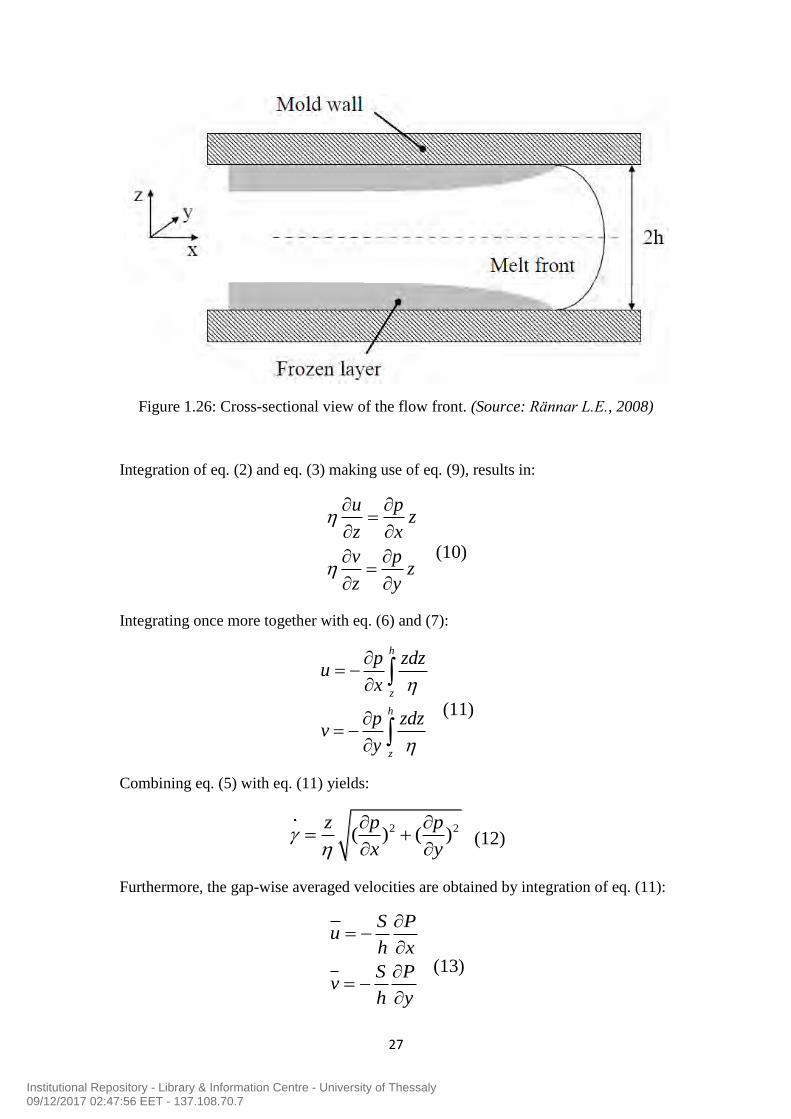
Figure 1.26: Cross-sectional view of the flow front. (Source: Rännar L.E., 2008)

Integration of eq. (2) and eq. (3) making use of eq. (9), results in:

u pz

z x

v pz

z y

(10)

Integrating once more together with eq. (6) and (7):

h

z

h

z

p zdzu

x

p zdzv

y

(11)

Combining eq. (5) with eq. (11) yields:

2 2( ) ( )z p p

x y

(12)

Furthermore, the gap-wise averaged velocities are obtained by integration of eq. (11):

S Pu

h x

S Pv

h y

(13)


28

where S is called the flow conductance or fluidity (the ease with which a melt can be

forced through a mold):

2

0

( , )( , , )

hz

S x y dzx y z

(14)

where is the local viscosity and h is half the height of the gap. Substituting eq. (13)

into eq. (1) gives:

( ) ( ) 0p p

S Sx x y y

(15)

The viscosity varies across the gap thickness, as well as spatially in the x and y

directions. It may also depend on the strain rate and temperature.

Note: The Hele-Shaw flow model is valid distant from the gate and from the active

flow front. In these regions, the flow is governed by a boundary layer problem, in

which the layer is approximately equal to the thickness of the gap. At the flow front,

the flow field is considerably more complex, because of the existence of the fountain

flow effect. Moreover, another breakdown of this model occurs when thick sections

are considered. Although most injection molded parts are thin in nature, there are

some that can have relatively thick regions. Because one of the founding assumptions

of this model is the thin section, error increases as the aspect ratio (b/L) of the

geometry increases. (Osswald et. al., 2001).

Note: In a general 3-dimensional steady fluid flow problem, one must solve for four

dependent variables: u, v, w and p, as functions of three independent variables: x, y

and z. However, for highly viscous fluids in a narrow gap, the Hele-Shaw formulation

allows to solve one partial differential equation (15), for one independent variable, p,

which only depends on x and y (p(x,y)). This is an enormous simplification for

modeling the injection mold filling (Dantzig & Tucker, 2001).

The viscosity can be described with different material models, and figure 1.27 plots

the viscosity according to three commonly used constitutive models: the Newtonian

model (eq.16), the Power Law model (eq.17), and the Cross model (Eq.18).

0 (16)

1nK (17)

0

1 ( )mC

(18)

where 0 is the zero shear viscosity, K is the consistency coefficient, n is called the

Power law index, is the infinite shear viscosity, m is a parameter called the Cross

rate constant/consistency constant and C is a constant related to the material.


29

Figure 1.27: The viscosity as a function of the shear rate for three different material

models. (Source: Rännar L.E., 2008)

1.12.2 Packing

In the packing phase, the mold is filled up by polymer melt. More melt is forced into

the mold in order to compensate for the volumetric shrinkage and therefore, a

compressible formulation is required to model this behavior. The governing equations

for this phase are the same as for the filling phase and consideration is taken to the

compressibility of the melt, by using a dependency of the specific volume on pressure

and temperature (v(T,P)). This is called the pvT relationship, which can be modeled

with different complexities.

Commonly used models for the processing of polymers are the Spencer-Gilmore

model, which is derived from the ideal gas law by adding a pressure and temperature

correction term to the specific volume, and the modified Tait pvT model with 13

parameters. Autodesk Moldflow Insight uses the Tait model (see PVT properties –

page 80). This model can predict the abrupt volumetric change for semi-crystalline

polymers and it is also suitable for amorphous polymers.

Lastly, it must be noted that the crystallization kinetics has an important effect on the

shrinkage and warpage of the final part. The crystallization of a material influences

the flow analysis, including changes in the modeling of viscosity, density/specific

volume, conductivity, elastic modulus, solidification, the inclusion of latent heat in the

energy equation, the orientation effect on shrinkage, etc. The model for crystallization

is usually expressed as the rate of crystallization as a function of other terms, such as

crystallization rate, temperature, crystallinity, cooling rate, etc.


30

1.12.3 Cooling

The objective of the mold-cooling analysis is to solve the temperature profile at the

cavity surface, using boundary conditions of polymer melt during filling and packing

analysis. When the injection molding process is in steady-state, the mold temperature

will fluctuate periodically over time during the process, due to the interaction between

the hot melt and the cold mold (figure 1.28). In order to reduce the computation time

for this transient process, a cycle averaged temperature T , that is invariant with time,

is introduced for the mold, but the transient state is still considered for the polymer.

Figure 1.28: Typical mold temperature variations. (Source: Rännar L.E., 2008)

The overall heat conduction phenomenon is governed by the energy equation:

2 2 2

2 2 2( )

mm p m

T T T TC k

t x y z

where ρm is the density of the mold, Cpm is the specific heat of the mold and km is the

thermal conductivity of the mold. The cooling phase of the process is described by

solving a steady-state Laplace equation for the cycle-averaged temperature

distribution throughout the mold:

2 2 2

2 2 2( ) 0m

T T Tk

x y z

where T is the cycle-average temperature of the mold. The second equation, together

with a simplified version of the first equation, where only the gap-wise coordinate is

considered, can be both used to predict the mold and part temperature, during cooling.


31

1.13 Heat transfer models

Injection molding, by nature, is a fully non-isothermal process. This means

temperature is non-uniform and that it depends greatly upon time and processing

conditions at any stage of the process. Energy in transferred via conduction and

convection, during the molding process.

Most simulation packages assume that the injection temperature is uniform and

constant. This is clearly not the case in actual injection molding, where fluctuations in

temperature can occur axially along the shot, as well as non-homogeneous

temperatures through the thickness of the shot. The uniform injection temperature

assumption is clearly not a result of inability of the computer simulation, however, but

it has difficulty in measuring the actual injection shot temperature. Therefore, the

uniform injection temperature is reasonable, for most calculations (Osswald et. al.,

2001).

- Because the material is injected through the gate, the higher shear rates cause

an internal heating of the polymer molecules. This heat generation is

commonly referred to as viscous dissipation. The molecular friction of

polymer chains rubbing against one another can cause a rather significant

temperature rise in the melt. This effect is readily accounted for by modern

simulation techniques.

- Additional heat transfer occurs due to the polymer flow in the form of

convection. The fluid motion transfers energy along its flow path and thus

convects heat, during mold filling.

- The last major mode of energy transfer, during the injection molding cycle,

arises because of conduction. Even though conduction occurs in all directions

of the polymer, the thin nature of injection molded parts causes conduction

through the thickness direction to dominate. Therefore, simulation programs

will typically only consider conduction across the thin gap. This simplification

is quite valid, when the low thermal conductivity of polymers is considered.

Because the mold wall is much cooler than the hot melt stream, conduction is

far greater into the mold than along the flow direction.

Note: Generally, one compounding effect that arises when molding semi-crystalline

polymers is the heat of crystallization or fusion. During the process of the crystalline

structure formation, a certain amount of energy must be conducted out of the material,

before the cooling process can continue.


32

2. Introduction to Autodesk Moldflow Insight (2012)

What is Autodesk Moldflow Insight ?

Autodesk Moldflow Insight (AMI) is a product suite designed to simulate the plastic

injection molding process and its variants, such as gas-assist injection molding,

injection-compression, thermosets processing, etc. AMI consists of a single common

user interface, called Autodesk Moldflow Synergy and a range of analysis products.

Together they provide an insight into the many and varied aspects of plastic injection

molding. It is therefore an essential tool for a wide range of users.

What is Autodesk Moldflow Synergy ?

Synergy is the graphical user interface for AMI. It provides a quick, simple method of

preparing, running and post-processing an analysis for a model. It also has fast and

easy to use wizards for creating multiple cavities, runner systems, cooling circuits,

mold boundaries and inserts. Included with Synergy is a material searching capability

for the extensive material database, too. Material creation tools exist to import,

change/modify and create materials to be used for any AMI analysis. To communicate

your results with colleagues, AMI has a report generation facility that creates reports.

Anyone can customize the reports to contain any of the results derived from an

analysis. The reports can contain images of the parts analyzed, including any of the

animated results. One report can contain results from any number of analyses or

studies.

2.1 Inside the graphical user interface

Synergy, shown in figure 2.1, is the environment used for pre-process, run and post-

process an analysis for all AMI analyses sequences and molding processes.

Figure 2.1: Autodesk Moldflow Synergy window.


33

Within Synergy, you can set up a sequence analysis (such as Cool + Fill + Pack +

Warp), run the analysis, view the results and prepare a report. Each section is

described in table 2.1.

Table 2.1: Main sections of Autodesk Moldflow Synergy.

Section Description

Quick Access Toolbar

Provides quick access to the functionality of AMI.

Contains group of commands commonly used. This can

be customized easily.

Environment tabs

Set of tabs which content depend on what is displayed in

the display area and the previous selections. Multiple

environment tabs can appear at a given time.

Context menu

Menu accessed with a right click that is context

sensitive. Different options appear depending on where

the cursor is when the context menu is activated.

Panels

Area on the side of the screen that contains panels used

for project, study, and layer management plus tools used

for geometry creation, mesh diagnostics and mesh

cleanup. A notes panel can be opened that has a section

for study notes, (stays with the model when copied) and

plot notes for each individual result plot.

Display

This is the area of Synergy where documents (studies)

are opened and models are shown.

Wizards

A wizard is a tool that helps you perform a specific

multi-step task.

2.2 Application Menu

The Application Menu can be accessed by pressing the button on the top left

corner of the interface. This menu expands and looks like that in figure 2.2. This

menu provides access to specific file related commands, such as: new, open/close,

save, export, print and study properties. You can access the application options from

this menu as well.


34

Figure 2.2: Application Menu.

2.3 Quick Access Toolbar

The Quick Access Toolbar, shown in figure 2.3, located at the top of the Autodesk

Moldflow Synergy window contains the most commonly used commands available in

Synergy.

Figure 2.3: Quick Access Toolbar.


35

2.4 Environment Tabs

The Environment tabs change depending on what is currently shown in the display

area and the previous selections. Figure 2.4 shows the Get Started environment tab

that you see when opening Autodesk Moldflow Synergy for the first time.

Figure 2.4: Environment tab - Get Started tab.

Multiple environment tabs can appear as a result of a selection. Once you are done

with the tasks accessible through such environment tab, just select finish/exit to return

to the previous parent tab. Examples of such environment tabs are shown in the

following images.

One can change the display of the environment tab at any time. Select any option

from the pull-down menu located at the top of the tab, as in figure 2.5.

Figure 2.5:

Environment tab display options

selection.


36

Table 2.2: Environment tabs available.

Environment

tabs

Function

Get Started

Creating, opening, importing projects and models. Access to

monitoring analysis running, access to tutorials, new features

documentation and the community.

Home

Importing, adding geometries and meshes. Setting the molding

process and analysis sequence, selecting the material, configuring

the process settings and all analysis prerequisites necessary for the

selected process. Monitoring analysis running, reviewing results

and creating reports.

Tools

Creating, importing and editing databases for materials and other

properties used in an analysis. The basic commands for the

Application Programming Interface (API) are listed here as well.

Geometry

(opened from

the Home tab)

Creating, duplicating or querying nodes, curves and regions,

creating runners, cooling lines, inserts or mold boundary with the

aid of Wizards, defining and activating a local coordinate system

or modeling plane, and diagnosing surface problems. Tools for

selecting entities and properties manipulation.

Mesh

(opened from

the Home tab)

Creating, refining, diagnosing, and fixing meshes. Tools for

selecting entities and properties manipulation.

Boundary

conditions

(opened from

the Home tab)

Adding or modifying boundary conditions to the model such as

injection locations, prohibited gate notes, Dynamic Feed, coolant

inlets, constraints and loads. Available boundary conditions

depend on the molding process selected.

Results

(opened from

the Home tab)

Setting display options for results, querying results and outputting

results to a file. The preferences for the plots properties can be

modified from this menu.

Reports

(opened from

the Home tab)

Creating, editing and viewing reports based on one or more

analyses. Notes, images and animations can be created from this

tab as well.


37

2.5 Panels

Creating, editing and validating a geometry or a mesh requires substantial interaction

with the part model. So does writing notes about a study or a result. The panel layout

provides an uninterrupted access to the part model in the display window and can

greatly improve user efficiency and productivity. The Project panel (figure 2.6)

displays either the Tasks or Tools tab.

2.5.1 Tasks tab

The tasks tab is divided into two sections:

Project pane.

Study tasks pane.

A divider bar between the Project pane and the Study tasks pane is movable, so the

relative sizes of the two panes can be changed at any time. The Tasks tab is shown in

figure 2.6.

Figure 2.6: Tasks tab on the

Projects panel in Synergy.


38

a) Project pane

The Project pane is the top level of organization in Synergy. It contains a list of all the

studies within a project. A project is equivalent to one “directory” on the hard disk,

with a collection of AMI analysis files. Within the Project pane, studies can be

organized into virtual “Folders” and any number of folders can be created to organize

studies within one project.

For each study in the Project pane, one or more icons may appear to the right of the

study name. These icons represent the types of analyses that can be run in AMI and

the status of a given analysis. Several icons can be grouped together to form an

analysis sequence such as , which indicates a Cool + Fill + Pack + Warp

analysis. Let’s assume that a Fill analysis is going to be run. When the analysis is over

and all the results are available for the study, the icon will appear. However, the

icon indicates that the selected analysis is a filling analysis, but has not yet been

completed, because it is not filled. If an analysis is aborted, the icon similar to is

shown instead. The red box with the “x” mark indicates that an analysis was started,

but not finished and the solver has stopped.

Studies

Studies are files that contain all the information about a part to run an analysis. The

extension is *.sdy. The study file contains:

Imported or created geometry.

Finite element mesh.

Analysis sequence.

Material information.

Injection location(s).

Process settings.

Figure 2.7:

Project Pane.


39

b) Study tasks pane

The Study Tasks pane displays a list of the basic steps necessary to set up and run an

analysis. The information shown in the Study Tasks list always relates to the currently

active study. The study tasks pane includes the following icons:

Table 2.3: Study Tasks Icons.

Icon Name Description

Translation model

Indicates the original file

format of the geometry.

Midplane model *

Indicates the model uses

midplane mesh technology.

Dual Domain model *

Indicates the model uses dual

domain mesh technology.

3D model *

Indicates the model uses 3D

mesh technology.

Analysis sequence

Shows the current analysis

sequence selected.

Material

Shows the current material

selected and provides access

to material searching

functions.

Injection nodes

Sets the injection location on

the part. Lists how many

injection locations are in the

model.

Circuits

Sets coolant inlet properties

and starts the circuit creation

wizard. Lists how many

cooling inlets are in the

model.


40

Process setting

Sets all the variables for the

analyses selected in the

analysis sequence.

Optimization

Launches a wizard for a

design of experiment (DOE)

analysis.

Start analysis

Starts the analysis or opens

the job manager with a right

click.

Results

Lists all graphical results.

Results folders

For each analysis sequence

there will be a result folder

under which the results are

grouped together.

Task done

Indicates that the task is

completed and information is

provided so an analysis can

be started.

* See ‘Mesh types’ below for more details.

In addition to all the tasks required to set up the study to the point where an analysis

can be run, there is also a listing of all results created once an analysis is completed.

An example of the Study Tasks list is shown in figure 2.8. In this example, all

analysis setup tasks have been completed, an analysis has been run, and results are

now ready for viewing.

Figure 2.8:

Study tasks list.


41

Mesh Types

Analyzing a model is a complex operation. Modeling the way molten plastic flows,

especially through complex model geometry, is difficult. In order to run an analysis,

one must have a meshed model. The mesh is a web that consists of elements, with

each element containing a node at every corner. The mesh represents the part shape

and provides the basis for the analysis, where molding properties are calculated at

every node. The selected mesh type, or analysis technology, determines which

molding processes and which analysis sequences are available for selection. The

analysis technology types supported by AMI are:

Midplane model: A mid-plane mesh provides the basis for the analysis. This

mesh consists of three-node, triangular elements that form a one-dimensional

representation of the part shape through its center, or mid-plane. The thickness

of the part is represented by a thickness attribute applied to the mesh elements.

The thickness of the part is stored in each element. The analysis then

incorporates this measurement, by dividing the thickness of the part into thin

layers, called laminaes. This provides a defined part volume on which

calculations can be performed. Midplane analysis technology is appropriate

when the part is predominantly thin-walled.

Dual Domain model: A surface mesh provides the basis for the analysis. This

mesh consists of three-node, triangular elements that form a one-dimensional

representation on each surface of the part. The mesh elements are matched

across opposing faces. The thickness of the part is determined by the distance

between the opposing faces. The model could be visualized as a hollow body

covered with a surface shell. Dual Domain analysis technology is appropriate

when the part is predominantly thin-walled.

When analyzing a part, the volume of the model is represented by thin layers

through the thickness of the part (typically 10 or more layers through the

thickness, i.e. laminaes). Elements on the opposite faces of the part must be

matching so the layers can be built. These matched elements ensure the

alignment of the layers through the thickness. These layers enable an accurate

representation of thin, cross-sectioned parts, where there is a rapidly changing

characteristic profile, for example, temperature, and flow-front velocity.

Note: The number of laminaes (layers) across the thickness defines the number of

divisions that the plastic cross-section is broken into.


42

3D model: A volume mesh provides the basis for the analysis. This mesh

consists of solid, four-node, tetrahedral (tetra) elements; each tetra has four

triangular faces and six sides. Therefore, a 3D mesh represents the CAD

model, by filling the volume of the model with tetras.

3D meshes work well for parts that are thick/chunky or solid, because tetras

give a true 3D representation of the model. A 3D analysis does not make the

assumptions that are made for Midplane or Dual Domain analyses. Thus, 3D

analyses often require additional computational time to complete. This makes

a 3D mesh more appropriate for thick models with complicated shapes, while

Midplane and Dual Domain meshes are more applicable for thin-walled, shell-

like parts. Furthermore, a tetrahedral mesh does not require a thickness

property, as it is true volume-filling mesh. Of course, when a more detailed

analysis is needed, such as studying of the fiber orientation of a fiber filled

material, then a 3D mesh will be the best choice.

Furthermore, in the project pane, the type of technology used for each model is

identified with the icons located to the left of the study name. Midplane is represented

with (yellow icon), Dual domain with (blue icon) and 3D with (red icon).


43

2.5.2 Tools tab

Modeling and meshing tools can be found on the Tools tab in the Project panel. The

part model remains visible in the display window without being obscured by tool

dialogs, as shown in figure 2.9.

Figure 2.9: Tools tab in the Project panel.

Any of the model creation or mesh editing tools can be accessed easily, once you are

in the Geometry or Mesh environment tabs without having to navigate through the

Geometry or Mesh environment tabs every time you are in need of a new command.

Layers

Layers is a method of organizing the entities (nodes, elements, regions, etc.) in your

model into groups, and then controlling the visibility and display properties of the

entities on a per-group basis. The use of layers is very handy when modeling, fixing

the mesh or during results visualization. For a model that has been meshed, there will

be several default layers, including: Default Layer, New Nodes, and New Triangles.

There will also be one or two layers for the imported geometry. Layers can also be

organized to represent geometries, such as runners, gates, edge, top, side, etc. The

Layers pane is by default, located under the Tasks/tools pane. The layers pane can be

a floating dialog. To make the pane float, simple click in the icon area of the pane and

drag it of the panel.

In the layers pane shown in figure 2.10, several details can be seen including:


44

The bold layer is the active layer. Any new geometry that you create, for

example a runner system, will be added to this layer.

The layers with a tick in the check box are visible layers. All entities

assigned to those layers will be visible on the screen.

The highlighted layer with the blue background is the

currently selected layer. Most of the layer commands work on the highlighted

layer, as illustrated in figure 2.10.

A complete list of commands and actions available for layers are shown in table 2.4

below.

Table 2.4: Layer icons.

Icon Command Action

Create Layer Creates a new layer. Once created, one may

click on the name to change it.

Delete Layer

Deletes the highlighted layer. If there are

any entities on that layer, one will be

prompted to delete the entities or to move

them to the active layer.

Activate layer Makes the highlighter layer active. The

layer name becomes bold.

Layer Display

Allows one to view and edit the color and

display methods of entities on the

highlighted layer. It also provides the

option to hide/show entity labels, for

example element or node numbers.

Assign Layer Assigns the currently selected entities in the

display window to the highlighted layer.

Adds entities to the highlighted layer by a

number of levels. If there is only one

Figure 2.10:

Layers Pane.


45

Expand Layer

element on a layer, and the expand

command is used, all of the elements

attached to the single element are added to

this layer, as well as all of the nodes on the

elements . The expanded elements

can also be moved to a new layer, so there

is a layer for the original elements to be

expanded and the layer containing the

expanded entities.

Clean Layers Deletes all layers with no entities on it.


46

3. Working in Synergy

In this topic the import of a CAD model is going to be examined, as well as the way it

can be meshed, the cleanup/repair of the mesh that comes after and how to prepare the

model, so that it can be ready for analysis.

3.1 Designing the model

The goal was to study the case of a center-gated disk (thin-walled part), filled with a

fiber reinforced material. So the first step was to create a disk with dimensions of: R =

radius = 65 mm and h = thickness = 2 mm. This is where the Autodesk Inventor

Fusion is helpful. Inventor Fusion is 3D mechanical CAD design software, for

creating 3D digital prototypes used in the design, visualization and simulation of

products.

Step 1:

Ensure the ‘Solid’ option from the ‘Modeling’ tab, on the top left of the screen, is

selected. Define the plane on which the model will be designed. This is done through

the ‘Origin’ command on the left. The disk under study will be designed on the XY

plane, as shown in figure 3.1 with green color. Remember the plane on which the

model was initially created. It will be of great importance later on. Choose the

‘Cylinder’ option from the ‘Solid’ tab. Now the only thing missing is the

dimensioning of the solid cylinder.

Figure 3.1: Selecting the cylinder option and the design plane.

Step 2:

Move the mouse on the red spot and from there one can specify the radius of the

cylinder, as shown in figure 3.2. Type 65 (mm) and then double press ‘Enter’. Right

after, one should define the height/thickness of the cylinder and that is done through

the command ‘Extrude’, which will appear automatically as a small yellow dart, right

after the radius is defined, as shown in figure 3.3. So type 2 (mm) and double press

‘Enter’ again. The steps described are shown in figures 3.2, 3.3 and 3.4.


http://en.wikipedia.org/wiki/Computer-aided_design

47

Figure 3.2: Specifying the radius of the circle.

Figure 3.3: Specifying the thickness of the cylinder.


48

Figure 3.4: Presentation of the final model.

Step 3:

The model is ready for import. Now just save the work and click on the ‘Simulation

Moldflow Insight’ command (figure 3.5). This will automatically create a .sat file

(Standard ACIS Text). Save this file in a folder, because this is the file one will need

to import in AMI.

Figure 3.5: Sending the file to Autodesk Moldflow.

3.2 Importing the model

Step 1:

Now it is time to open the AMI program. First create a new project with a specific

name and save it in a folder. This project can contain lots of studies and every change

that is made on the studies, will be saved in this folder. So now import the .sat file,

which was created earlier, and the following window dialog will appear.


49

Figure 3.6: The import dialog. Choose the Dual Domain mesh type and the Process

using Autodesk Moldflow Design Link option (AMDL).

When importing a solid model, always choose Dual Domain (here) or Midplane. If

someone eventually wants to work with a midplane or 3D model, initially import the

CAD model as Dual Domain, study the model and clean the mesh up as necessary.

After the model is cleaned up, the mesh type can be changed/converted and re-meshed

with the new desired format.

Step 2:

Click on the ‘Advanced…’ option in the lower right corner. AMDL creates a dual

domain or 3D mesh directly from the CAD kernel. This results in a better solution that

provides better fidelity, better scaling and the ability to handle multi-component

models.

Global edge length (GEL): allows setting the target element edge length when

the mesh is generated. This value is the main control for the mesh density of a

part. The GEL should be about 2 times or less, the nominal wall thickness for

a 3D mesh, and 2 to 5 times the nominal wall thickness for a Dual Domain

mesh.

Because the thickness of the disk is 2 mm, the GEL for this dual domain

analysis is set to the minimum (for more elements, therefore better analysis),

that is: (2 x h) = 2 x 2 = 4 mm, as shown in figure 3.7.

Chord angle: when tightly curved sections of the model are not meshed

adequately, one can increase the mesh densities in these areas by defining a

chord angle. This controls how closely the curve of the CAD model is

approximated by straight section in the mesh. The smaller the chord angle, the

shorter the chord length, the finer the mesh.


50

When prediction of weld lines is critical or hesitation effects and air traps must

be correctly predicted, a finer mesh is preferred over a coarse mesh. In this

specific example, the chord angle is set to 41 degrees, as shown in figure 3.7.

Mesh on assembly contact faces: There are 3 different options available here

for the meshing of the surfaces of assemblies that come into contact. Here the

«Fault Tolerant» option is selected. This helps in repairing any minor errors in

the CAD model. Mesh nodes are matched where possible. Some mesh

adjustments may be required to match nodes on contact surfaces.

Silver removal: A silver is a small feature that is usually found at CAD surface

join boundaries. Silvers can result in small mesh elements with high aspect

ratios. It would be better for them to be removed.

Figure 3.7: Import Options.

Step 3:

Press OK twice. The model will be meshed with the desired values and the final result

is shown in figure 3.8. A total of 4772 elements were created.


51

Figure 3.8: Presentation of the disk in the Dual Domain mesh.

3.3 Preparing the model for analysis

This section of course is going to be very extensive, as one should focus on details

that will make the final results of the injection molding process more accurate and

acceptable.

3.3.1 Assignment of properties

Select the whole part. Right click and choose ‘Properties’. A new window will pop

up, like the one in figure 3.9. The first option will select the front and the back side of

the disk, while the second option will select the circumference of the disk. Select both

properties that appear in this window (holding down CTRL) and click OK.


52

Figure 3.9: Selecting the whole disk’s surface.

In the ‘Part Surface Properties’ tab, one can decide how the thickness in the part will

be represented. Here a common value of 2 mm for the whole surface of the part is

chosen (uniform thickness), as shown in figure 3.10.

Figure 3.10: Assigning a common thickness for the whole disk.


53

The ‘Mold Properties’ tab, is used to specify the properties of the mold block in

contact with the selected elements or regions of type part surface (dual domain). Here,

one can define on which side the cavity and the core will be assigned and specify if a

local mold material different from the one used in the process settings, is going to be

used. For this study, the top side is chosen as the cavity side and the mold material

remains the same (figure 3.12). In figure 3.11, one can see the standard mold and how

simply designed it is. Nothing more complex than that is needed to mold a part with a

very simple geometry, like a disk.

Figure 3.11: A standard mold. The fixed/stationary half is usually called cavity or A-

half. The moving half is commonly referred to as core or B-half. The cavity side is the

one that “includes” the feed system. [4]

Figure 3.12: Specifying the cavity side and whether the same or a

different mold material is going to be used.


54

The ‘Mold Temperature Profile’ tab, is used in the Fill + Pack analysis. Unlike the

conventional injection molding process, in which the mold is maintained at a near-

constant temperature, newer techniques utilize a variable mold temperature. The mold

is maintained at a hotter temperature during the filling phase, so as to facilitate and

achieve smooth surface appearance. During the packing and cooling phases, the mold

switches to a much cooler temperature to assist in freezing the part and decreasing the

cycle time. The time must be set in ascending order. Keep in mind that temperature

profiles cannot be set on hot runner elements. The profile used in the case of the

center-gated disk is shown in figure 3.13.

Figure 3.13: Specifying the mold surface temperature profile of the disk, with a

constant temperature of 80 °C. This temperature is not randomly selected, as it is the

optimum temperature for the material that is going to be chosen later on,

recommended by the manufacturer.

3.3.2 Modeling of the feed system

It’s always advisable to rotate and check the model for any inconsistencies. In the case

of the disk, the geometry is very simple, so no problems are expected. However, one

can examine in detail the resulting mesh for any possible errors/faults, though the

‘Mesh Repair Wizard’ option.

In this topic, the creation of the feeding system is going to be analyzed. Center-gated

disk, as the name implies, is a disk gated right in the center. A center-gated part is

reasonably well-balanced, but not as good as an end-gated part. The flow front starts

out to be radial and then straightens out and becomes linear. A center-gate location is

better for round or square parts.


55

For many cylindrical or symmetrically shaped parts, such as buckets, tubs, helmets,

boxes, cups and disk-shaped objects, a direct (or sprue) gate is the most common

choice. Before we proceed on with the analysis of the gate design, it would be better

to explain what a direct gate is.

Gates can have many different configurations, but they are broadly classified based on

the method of gate removal, into manually trimmed and automatically trimmed gates.

Manually trimmed gates usually require an operator to separate the parts from the

runners, during a secondary operation. The direct gate falls into this type of gates.

Manually trimmed gates are used for the following reasons:

The gate is too large to be sheared from the part as the tool is opened.

Some shear-sensitive materials, such as PVC, should not be exposed to the

high shear rates inherent to the design of automatically trimmed gates.

Simultaneous flow distribution across a wide front to achieve specific

orientation of fibers or molecules often precludes automatic gate trimming.

Sprue gating is different from almost any other type of gating and refers to the cases

where there is no traditional runner system or conventional gate. The part is gated

directly from the sprue. It is commonly used in single-cavity molds, where the sprue

feeds material directly and rapidly into the cavity with minimum pressure drop. With

a cold sprue there is no traditional gating. It is generally not considered a good gate

design, as the cross-section is larger than the part’s wall thickness and it is prone to

control the cycle time and over-pack the part. The disadvantage of this gate type is the

gate mark left on the part surface, after the sprue is trimmed off. Freeze-off is

controlled by the part thickness, rather than determined by the gate thickness.

Typically, the part shrinkage near the sprue gate will low; shrinkage in the sprue gate

will be higher. This results in high tensile stresses near the gate.

As far as dimensioning is concerned, the starting sprue diameter is controlled by the

machine nozzle. The sprue orifice diameter here must be about 1 mm larger than the

nozzle exit diameter. Standard sprues can have tapers from 0.5 degrees to 1.5 degrees

(1.0 degrees to 3 degrees included angle, see figure 3.14 – on the left), with a common

size of about 1.2 degrees taper angle, as shown in figure 3.14 – on the right.

Therefore, the sprue’s orifice diameter and length will control the diameter of the

sprue where it meets the part. Typically, the sprue diameter will be well over double

the wall thickness of the part, controlling the molding cycle time.

A small taper angle (a minimum of 1 degree) risks not releasing the sprue from the

sprue bushing on ejection. A large taper angle wastes material and extends the cooling

time. In most cases the sprue’s length should be kept as short as possible, too,

enabling rapid mold filling and low pressure losses.

Pressure loss is high in the sprue. This is the only place in a feed system where the

channel progresses from a smaller area to a larger. Frequently, smaller orifices are

used on long sprue bushings in an effort to reduce the mass. This results in extreme

high injection pressure losses, making the part hard to fill (Engelmann & Dealey,

1999). Smaller starting diameters demand much higher clamping forces.


56

In AMI there are three ways for the dimensioning of a cold sprue. One is to give the

sprue a non-tapered shape, just by specifying the diameter. Another way is to create a

tapered sprue with start and end dimensions.

The third way is to create a tapered sprue again, but this time one should define the

start diameter and the tapered angle. When the third way is chosen, one should have a

global view of how big the diameter of the sprue, where it meets the part, is going to

be.

For example, if a pretty big orifice diameter is used and a common tapered angle is

also used, it is certain that mesh problems will appear, such as intersections, between

the beam and the triangular elements (dual domain). Of course these can be fixed, but

not automatically. A manual repair of the model is required. Sometimes the mesh

repair is not an easy job. This is where the following equation helps in the

understanding of how big the contact diameter is going to be. The equation is

(Engelmann & Dealey, 1999):

2 1 tan( )d d L (1)

where: d2 = the end diameter

d1 = the start diameter (orifice)

L = the length of the sprue

φ = the included angle (note that in AMI: included angle = 2 x tapered angle).

Figure 3.14: A sprue gate can be modeled in AMI with beam or tetrahedral elements.


57

Figure 3.15: Designing principles of a direct gate. Average sprue lengths vary from

2’’ to 3’’ (51 – 76 mm). [5]

So with the role of a sprue gate explained, it is time to move on with its creation.

Initially select the front view and zoom all the way in (scale < 10 mm). Open the

Geometry tab and go to the ‘Create’ tab. Select ‘Nodes > Node by Coordinate’. Here

one can define a new node. In our case, a node right in the center of the part is needed

and that is a node with coordinates: (0, 0, 2). Click apply. A small blue node will

appear, like the one in figure 3.16.


58

Figure 3.16: Defining the initial (base) coordinate.

The next step is to offset this node. Select ‘Nodes > Node by Offset’. Once the new

window pops up, in the base coordinates box, select the node that was created right

above (this will be the reference node) and in the offset box, type the coordinates: (0,

0, 45). Click apply and then close. This will make a new node, 45 mm higher in the z-

direction, as shown in figure 3.17.

Figure 3.17: Creating the second node. The coordinates of the new node are now:

(0, 0, 47).


59

Now select ‘Curves > Create Line’. A new window pops up. Keep in mind that in the

input parameters, the top node (0, 0, 47) should be selected first and the base node (0,

0, 2) should be selected right after. Otherwise, the sprue will be tapered from the

bottom to the top.

In the ‘Create as > Modeling entity’ box, create a cold sprue with a start diameter of 3

mm and a tapered angle of 1.1 degrees. Also, in the ‘Mold Properties’ tab, use the

same material and in the ‘Mold Temperature Profile’ tab , use the same profile as the

one in figure, with a constant temperature of 80 °C. Press OK several times and then

click apply and close. A green line will be created, connecting the two nodes. The

steps described are shown in figure 3.18.

Note: One is able to understand how big the end diameter is going to be, using

equation (1). Therefore:

d2 = d1 + L tan (2.2o) = 3(mm) + 45(mm) 0,0384 = 3 + 1.729 = 4.73mm

Figure 3.18: Defining the necessary properties of the sprue gate.

The final step is to mesh this green line. Open the ‘Mesh’ tab and select the ‘Generate

Mesh’ command. Create a new mesh with a GEL of 4 mm again. Use a merge

tolerance of 0.01 mm and a chord height of 0.4 mm. Ensure the match mesh option is

checked, as well as the smooth mesh (NURBS Surfaces only) option. Before the

‘Mesh Now’ button is clicked, be sure to have deactivated the ‘Remesh already

meshed parts of the model’ option, otherwise the program will create a new mesh all

over from the start for the whole part, including the line. The steps are shown in figure

3.19.


60

Merge tolerance: Sets the minimum distance between nodes that AMI will aim

for (0.01 mm here), when it generates your Midplane or Dual Domain mesh. If

adjacent nodes are closer together than this distance, nodes will be merged

together during mesh creation.

Match mesh: Allows you to align the mesh elements on the two corresponding

surfaces of a Dual Domain mesh. A better mesh match increases thickness

accuracy and leads to more accurate analysis. Sometimes, activating mesh

matching will create thin high aspect ratio elements, called silvers. Although

the match ratio will be much higher, there may be some silvers that need to be

cleaned up. For dual domain meshes that will be converted to 3D, it would be

better to have this option unchecked. For dual domain meshes, match mesh

should be checked.

Chord height control and chord height: This check box and text box will

ensure that curved features have a mesh on rounded features. Without the

chord height control, some surface curves, such as fillets, degrade when

meshed.

Chord height control is effective only with parts that have curved surfaces.

Keep the value of the chord height somewhere in the range of 5-25% of the

used global edge length. If the value is below approximately 5%, the resulting

mesh tends to contain several long and/or thin triangles. If the value exceeds

25%, the chord height control has little effect. For the center-gated disk a 10%

of the GEL has been used, that is: (0.1 x 4) (mm) = 0.4 mm.

Smooth mesh (NURBS surfaces only): this option shifts the position of nodes

around to produce a lower average aspect ratio. It should be checked.

Figure 3.19: Right before the meshing of the sprue gate.


61

When the desired values have been correctly entered, click ‘Mesh Now’. The result is

shown in figure 3.20. Of course, someone can use a smaller GEL for the modeling of

the sprue gate. But there is no need to do that in a dual domain analysis. A smaller

GEL is going to be used for the whole part, when the conversion to a 3D mesh will be

made.

All to do now is check the whole mesh for any errors, such as overlaps, intersections,

high aspect ratios, etc. In table 3.1, a summary of all the mesh requirements is shown

for the three different mesh types: Midplane, Dual Domain and 3D. In any case, one

should check that these requirements are fully satisfied.

Figure 3.20: The feed system of the part is ready.


62

3.3.3 Mesh examination

Table 3.1: Summary of mesh requirements for the three mesh types.

Mesh Issue Dual Domain 3D Midplane

Free edges Must NOT have

any

Same as dual

domain

Can have at

boundary of holes

and parting line

Non-manifold

edge

Must NOT have

any

Same as dual

domain

Are valid at "T"

cross-sections,

e.g. ribs

Manifold edge Only type of edge

allowed

Same as dual

domain

Most common

type of edge

Match ratio

> 85% for flow

and > 90% for

warpage

Not applicable Not applicable

Reciprocal

Match > 90% for warpage Not applicable Not applicable

Aspect ratio Average < 3:1 and

Maximum < 6:1

< 30:1 on dual

domain mesh,

before

conversion to

3D

Same as dual

domain

Connectivity

regions

One group for the

part

Same as dual

domain

Same as dual

domain

Element

orientation

The top (blue) side

of the element

pointing outward

Same as dual

domain

Consistent mesh

orientation

Intersections Must NOT have

any

Same as dual

domain

Same as dual

domain

Overlapping

elements

Must NOT have

any

Same as dual

domain

Same as dual

domain

Zero area

elements

Must NOT have

any

Same as dual

domain

Same as dual

domain

Thickness

representation

Thicknesses

properly modeled Not applicable

Thickness

properly assigned

Inverted tetras Not applicable Must NOT have

any Not applicable

Collapsed faces Not applicable Must NOT have

any Not applicable

Number of 3D

layers Not applicable

6 layers

typically OK, 8

layers for fiber

orientation or

gas-assist

Not applicable


63

Internal long

edges Not applicable < 2.5:1 Not applicable

Extremely large

volumes Not applicable < 20:1 Not applicable

High aspect

ratios Not applicable < 50:1 Not applicable

Small angle

between faces Not applicable > 2 degrees Not applicable

Large angle

between faces Not applicable < 177 degrees Not applicable

Through the ‘Mesh Repair Wizard’ one should check for any possible errors that

might have occurred. Unfortunately, in the case of this center-gated disk, some errors

did occur. Specifically 3 intersections were detected. But they can be fixed.

So the first step is to open the ‘Mesh’ tab and go to ‘Mesh Diagnostics > Overlap’. On

the left of the AMI interface the ‘Overlapping Elements Diagnostic’ has been

activated. So check the ‘Place results in diagnostic layer’ option.

This will create a new layer in the layers pane. Click on the ‘Show’ button and then

‘Close’. Figure 3.21 shows the regions that must be fixed.

Figure 3.21: Three (3) intersections were detected by the Mesh Repair Wizard.


64

So now move to the layers pane and right click the ‘Diagnostic results’ option. Select

the ‘Hide all other layers’ option and right after click on the ‘Expand Layer’ button.

Bring forth the back side of the disk and zoom in (figure 3.22). With the yellow

colored circles are pointed out the two nodes that caused the mesh problem. The

appearing intersections can easily be fixed, using the ‘Merge Nodes’ command.

So in the new ‘Merge Nodes’ window that appears, choose node 2 (N15634) as the

node to merge to and node 1 (N8142) as the node to merge from. Click apply and then

close. This will repair the mesh and the final result is shown in figure 3.23.

Figure 3.22: Specifying the cause of the mesh problem.

Figure 3.23: Intersections all repaired.


65

Notice the red colored circle in figure 3.23. The specific node (N8610) needs to be

smoothed. With the help of the ‘Smooth Nodes’ option, select this node and click

apply. Be sure to have activated the ‘Preserve feature edges’ option. The mesh is now

completely fixed, as shown in figure 3.24. In order to make the model appear in its

original form again, right click on the ‘Diagnostic results’ option and now select the

‘Show all other layers’ option.

Figure 3.24: Mesh repair is finally ready.


66

Figure 3.25: Summary report about the current dual domain mesh (using Mesh

Statistics). All mesh requirements are more than satisfied, according to table 3.1.

The final step will be completed when the injection location is set. Zoom in on the top

of sprue and place an injection location (a yellow cone) on the blue node. This will

ensure that the injection location is set right in the middle. An injection location is

always necessary, as it specifies the point from which material is going to be fed into

the sprue gate, therefore the cavity. Everything is ready now, as shown in figure 3.26.

Notice that no ventilation system exists. In order to define one, a pair of cooling

circuits must be created. This will prevent the creation of air traps in our part. In this

study, a Fill + Pack analysis has been run. So some air traps are expected to appear in

the circumference of the disk. However, this is not a crucial problem for the final

results. In the next topic, the process settings will be analyzed.


67

Figure 3.26: Injection location is set. Material will now be injected into the cavity

from the top of the sprue. The elements now are 4783 in total (including the 11 beam

elements of the sprue gate).

Figure 3.27: A real center-gated disk, with a diameter of 177.8 mm and thickness of 3

mm. (Source: Kunc et. al., 2007)


68

Now let’s assume that a complex geometry needs to be studied. In this case a more

dense mesh is required. Using a very small global edge length (GEL) when converting

from a dual domain to a 3D mesh, won’t solve the problem. The number of elements

will certainly increase when the 3D mesh is used, however, not to a big extent. In

order to achieve a very high number of elements, thus better analysis, but much

greater computational time, one should import the model through the AMDL with a

rather small GEL. Remember that when the disk was imported, a GEL of 4 mm was

used. According to AMI theory, in a Dual Domain analysis the minimum GEL that

should be used is two times the part thickness.

But what will happen if the GEL is reduced ? For example, if a GEL of 2 mm or even

less is initially used, then the elements in the Dual Domain mesh will be dramatically

increased. Therefore, one can imagine how many elements will be created in the 3D

mesh. The following figures show the resulting mesh.

Figure 3.28: Presentation of the disk in a dual domain mesh, using a GEL of 2 mm. A

total of 19204 elements were created. Notice how the appearance of the top surface

has changed.


69

Figure 3.29: Presentation of the disk in a 3D mesh, using a GEL of 2 mm again and 8

layers through thickness (3D conversion will be discussed later). A total of almost

224853 elements were created.

Figure 3.30: Presentation of the disk in a dual domain mesh, using a GEL of 1 mm. A

total of about 71888 elements were created. That’s too many for a dual domain mesh.

Notice how the appearance of the top surface has changed again. The elements are

very densely packed.


70

Figure 3.31: Presentation of the disk in a 3D mesh, using a GEL of 1 mm again and 8

layers through thickness (3D conversion will be discussed later). A total of almost

856522 elements were created.

Although the 3D conversion is discussed much later in detail, it would be useful to

point out again that in the original study a GEL of 2 mm (equal to the thickness of

the disk) was used, when converting to 3D. The elements created were almost

55000. That’s about 4 times less elements, compared to those created when a GEL

of 2 mm was used to import the model initially and convert to 3D later (figures

3.28 & 3.29).

Observing figures 3.28 to 3.31, one can conclude that the elements in a 3D mesh

are almost 12 times more than those in a dual domain mesh, using of course the

same GEL for the creation of both and 8 layers through thickness (for the 3D

conversion). Using even more layers in the thickness direction would increase this

ratio dramatically.


71

4. Process Settings

4.1 Molding Material dialog

First thing to always check is the ‘Molding Process Setup’ environment tab. The

‘Thermoplastics Injection Molding’ option should be selected. After this, one can

choose the appropriate material for the study. There is an extended material library

and with the search button one can find almost any desired material. For the case of

this center-gated disk, a 30% short glass fiber (SGF) reinforced polybutylene

terephthalate (PBT) has been selected. PBT is a thermoplastic engineering polymer.

The material’s trade name is Crastin HR5330HF NC010 (Moldflow Verified), from

DuPont Engineering Polymers manufacturing company. The material’s structure is

crystalline.

But why is the phrase ‘(Moldflow Verified)’ included in the material’s name? This

stands for the fact that the specific polymer has undergone testing by experts.

Confidence in simulation results comes from knowing that the material used, will

result in accurate analysis predictions. The Autodesk Moldflow Plastics Labs perform

multiple injection molding trials and compare analysis predictions with in-mold

performance.

Plastic materials are widely used as metal replacement in industrial applications,

owing to the advantages of higher strength-to-weight ratio and high corrosion

resistance. Glass and carbon fibers are commonly added into plastics to reinforce the

mechanical and thermal properties, with negligible change of weight. The addition of

fibers introduces anisotropy of the properties in injection-molded parts, mainly due to

the preferential orientation of fibers induced by the flow during processing. For

example, shearing flow, which is usually dominant during injection-molding

processing of a thin part, tends to align fibers in the shearing direction. The part is

much stronger and stiffer in the direction along which most fibers are aligned than in

the direction crossing the major fiber alignment. In order to determine the properties

in injection-molded parts and aid the design of mold and part and the selection of

processing conditions, the fiber orientation must be accurately predicted (Wang & Jin,

2010).

If the fibers are randomly oriented, the mechanical and physical properties will be

isotropic. If the fibers are aligned in one direction, the composite will be stiffer and

stronger in that direction compared with any other direction. The distribution of

orientations in a molded part could be quite diverse. One region may have random

fiber orientation, while others may have preferred alignment in certain directions.

In the injection molded short fiber composites, a characteristic layer structure is

observed, with the fibers oriented in quite different manners according to their

location through the thickness, as demonstrated in figure 4.1.


72

Figure 4.1: Schematic diagram of molding indicating the fiber orientation in the skin

and core layers. (Source: Somjate Patcharaphun, 2006)

Figure 4.2: Optical photomicrograph showing the fiber orientation pattern across the

thickness of a tensile test bar. (Source: Somjate Patcharaphun, 2006)


73

In the skin region, fiber orientation is predominately parallel to the flow direction.

This is due to, as the melt fills the mold, there is fountain flow which initially orients

the fibers perpendicular to the main flow direction. Fountain flow causes the melt to

be deposited on the mold wall with the alignment direction parallel to the mold fill

direction. Here, it solidifies rapidly and this alignment is retained in the solid article.

Further behind the melt front, shear flow dominates and produces fairly uniform

levels of fiber alignment. In contrast, the core of the molding contains fibers mainly

aligned perpendicular to the flow direction, due to a slower cooling rate and lower

shearing. Moreover, fountain flow does play a role in the development of the fiber

orientation distributions, observed in injection molded fiber-reinforced parts (Bay &

Tucker, 1992). Its influence, however, is frequently overwhelmed by that of the shear

and extensional flows.

Fibers longer than 1 mm are generally considered as long fibers. As described above,

a SGF PBT has been selected, i.e. fiber’s length is < 1 mm. Usually, the fiber

alignment in the flow direction is smaller in long-fiber materials, than in short-fiber

materials in injection molded parts (Phelps & Tucker, 2009). The main flow direction,

in the case of a center-gated disk, is radial.

Currently, most programs and commercial software, including AMI, use the Folgar-

Tucker model (Folgar & Tucker, 1984) to predict the fiber orientation. However,

recent experiments, including measurements of fiber orientation in injection-molded

parts (O’Gara et al., 2003) as well as measurements of rheology of fiber suspension

(Sepehr et al., 2004), indicate that the FT model predicts much quicker fiber

orientation change with respect to strain than has been observed, and thus, usually

over-predicts the overall fiber alignment.

This is why the reduced strain closure (RSC) model is going to be chosen here.

Generally, the RSC model exhibits slower orientation kinetics than the FT model.

Again, it must be noted that the goal of this study is not a fiber analysis. The equations

behind each model and what they represent will be described later. First, one should

look into the properties of the selected material, such as the rheological and thermal

properties.

4.1.1. General features

Crastin HR5330HF NC010 is a high flow (HF), moderately toughened and hydrolysis

resistant (HR) thermoplastic polyester resin. Some of its features include good

chemical resistance, low viscosity, dimensional stability and good processability. It

offers excellent balance of properties between terminal pullout and impact resistance.

Used for: automotive applications, engineering parts, connectors, industrial

applications/parts, electrical/electronic applications and machine/mechanical

parts. Its processing method is through injection molding.

Recommended processing: the melt temperature should be in the range of 240–

260 °C and the mold temperature in the range of 30-130 °C, with an optimum

temperature of 250 and 80 °C, respectively. The material’s ejection

temperature is 168 °C.


74

Generally, PBT materials have fast crystallization rates, so the cycle times are

typically low.

4.1.2 Mechanical properties

Fiber orientation is one of the major factors that determine the mechanical (elastic)

strength as well as the stiffness of a molded part. Theories have been developed to

predict the mechanical properties of short fiber composites once the fiber orientation

distribution in the parts is known. To calculate the mechanical properties, all the

theories follow a two step procedure:

The properties of a unidirectional short fiber reinforced material are estimated.

These properties are then averaged across the laminaes according to the fiber

orientation distribution density.

The material’s mechanical properties are not of concern for this study. That’s why the

equations that are used for their calculation are not going to be described here. But

one should keep in mind that in AMI:

When matrix properties with materials that have anisotropic matrix data are

used, the Mori-Tanaka micro-mechanics model will be chosen by default.

If the ‘Do not use matrix properties’ or ‘Use 7 matrix properties’ option is

selected with materials that have isotropic matrix data, the Tandon-Weng

mirco-mechanics model will be chosen by default.

Note: Matrix is the polymer without the fibers/filler present. The matrix + fibers/filler

make the composite material.

In this study the option ‘Use 7 matrix properties’ has been selected. Alpha1 defines

the thermal expansion coefficient in the flow direction and Alpha2 the thermal

expansion coefficient in the transverse direction (figure 4.3). By default, the Tandon-

Weng model has been selected for the analysis of the disk.

General Note: In order to modify the properties of a material go to ‘Molding Process

Setup’ tab and from there: ‘Advanced Options > Molding Material > Edit’.

Everything can be changed from there.


75

Figure 4.3: Mechanical properties tab. If a property name is shown in red, it

indicates that the property has not been tested for this specific material.

However, material data from the testing of a comparable generic grade was

found to be suitable and has been assigned to this material.

4.1.3 Shrinkage properties

Before the shrinkage prediction method is described, one should first select the

appropriate shrinkage model for the flow simulation. And this is very important, as it

can improve the shrinkage results to a big extent. As shown in figure 4.4, the

‘Corrected residual in-mold stress (CRIMS)’ model is selected by default and it must

be left as it is. Generally, CRIMS model is selected when shrinkage testing has been

performed on the material. This model is more accurate, because it is obtained by

correlating actual shrinkage tested values (figure 4.5) with the Fill + Pack analysis

predictions.

The ‘Uncorrected residual stress’ model will be selected when there is no shrinkage

data available for the material. The ‘Residual strain’ model is selected for those

materials where the CRIMS model was found inadequate to describe the shrinkage

behavior of the material.


76

Figure 4.4: Selecting the correct shrinkage model. Notice that the ‘RSC Fiber model

set’ option is also selected. As mentioned above, in this study the RSC fiber

orientation model will be chosen.

For the Crastin HR5330HF NC010 material selected for this study, a shrinkage test

has been already made, in order to ensure more accurate predictions. The following

observed shrinkage data were acquired through the Non-contact metrology (2D)

method.

Table 4.1: Shrinkage data for Crastin HR5330HF NC010.

Observed

nominal

shrinkage

Observed

shrinkage

Parallel 0.222 % Min. Parallel 0.190 %

Perpendicular 1.469 % Min.

Perpendicular 1.251 %

Max. Parallel 0.273 %

Max.

perpendicular 1.813 %


77

Figure 4.5: The shrinkage molding summary. This table contains the measured in-

plane shrinkage, parallel and perpendicular to the flow direction, under a range of

different injection molding conditions, such as packing pressure and melt-mold

temperature.

For injection molded parts, the part is constrained in the mold. During the

solidification of an injection molded part, shrinkage of the solidified layer is

prevented by two mechanisms. Once the part is ejected from the mold, these residual

stresses will be released in the form of shrinkage deformation. The mechanisms are:

a) Adhesion to the mold walls restrain (at least the outer skin) of the solid layers

from moving, and

b) The newly formed solid surface will be kept fixed by the stretching forces of

melt pressure.

In-cavity residual stresses (internal stresses) build up during solidification. Due to the

nature of constrained quenching, the residual stress distribution is largely determined

by the varying pressure history, coupled with the frozen layer growth. Once the part is

ejected from the mold, these residual stresses will be released in the form of shrinkage

deformation. If the initial strains, which are equivalent to the in-cavity residual

stresses, are uniform, the part will shrink uniformly without any warpage and post-

mold residual stresses. Warpage is caused by variations in shrinkage throughout the

part. Two types of shrinkage variations are considered:


78

a) Shrinkage variations from region to region (differential shrinkage effect):

For typical thin-walled parts, this form of shrinkage variation can be divided into

variations in the thickness direction of molded parts, mainly caused by the differential

cooling and variations from surface region to surface region

b) Shrinkage variation in different directions (orientation effect):

The difference between parallel and perpendicular shrinkage and anisotropic material

properties, relating to the fiber-orientation distribution, are one of the main causes of

part warpage for fiber-filled TPs.

Note: For fiber-filled TPs, reinforcing fibers inhibit shrinkage due to their smaller

thermal contraction and higher modulus. Therefore, fiber-filled materials shrink less

along the direction in which fibers align (typically the flow direction) compared to the

shrinkage in the transverse direction. Thus, the shrinkage in the direction of flow is

lower than the shrinkage perpendicular to the direction of flow. For the case of a

center-gated disk, the direction of flow is radial.

Figure 4.6: The mold shrinkage for a reinforced semi-crystalline polymer, such as a

glass-fiber reinforced PBT, varies with direction (flow vs. cross-flow) and with part

thickness. (The thickness of the disk is 2 mm or approximately 0.08 inches). [6]

The shrinkage of injection molded parts depends on the thermodynamic behavior of

the material during processing. For simplicity, a linear elastic behavior in the

solidified part and purely viscous behavior in the melt, is assumed.

It is reasonable to approximate the linear shrinkage using the following formulation:

( )o

r

T

i i

T

a T dT


79

where:

ai(T) = the linear thermal expansion coefficient (CTE) at temperature T in the i-th

principal direction,

To = the temperature when the local cavity pressure reached the atmospheric condition

(obtained from the flow simulation), and

Tr = the room temperature.

Right below, one can see the CRIMS model coefficients list. As mentioned earlier,

many materials in the Moldflow database have been “shrinkage tested”. This means

that the Moldflow Lab measured parallel and perpendicular shrinkage of moldings

molded with different parameters (usually rectangular plates). They also predict

shrinkages and some proprietary parameter ‘Tau’ (frozen shrinkage strain) for all

those regimes. After that Moldflow correlates the measured shrinkage with the

predicted shrinkage and ‘Tau’, as:

Shrink_parallel_exp = A1 Shrink_parallel_pred + A2 Tau + A3

and:

Shrink_perpendicular_exp = A4 Shrink_perpendicular_pred + A5 Tau + A6,

where “exp” stands for expected and “pred” for predicted.

The A1 – A6 coefficients are provided with the material database and their values are:

A1 0.310043

A2 -0.09543

A3 0.001911

A4 1.08717

A5 -0.114635

A6 0.002949

Note: The structure of a semi-crystalline material, when in the molten state, is

amorphous. However, as it cools, macromolecules tend to organize themselves

according to their own nature, i.e. they recover the primary crystalline percentage. In

the new reordered areas, the free space among molecules is lower than the amorphous

areas: a concrete specific volume reduction (“shrinkage”) occurs. So, semi-crystalline

polymers shrink more than amorphous ones; typically 0.5-1% vs. 1.5-5% depending

upon the particular material, because the crystals formed during cooling, take up less

volume than the unoriented (amorphous) molecules that exist during the melted phase.

This is the reason why amorphous TPs are less prone to warpage than crystalline

resins. While high shrinkage alone does not cause warpage, it increases the

probability that warpage will occur.

Furthermore, semi-crystalline materials have a sharp melting point, i.e. they transition

from solid to liquid very quickly over a short/narrow temperature range. This becomes

clear by observing figure 4.8. On the other hand, amorphous materials have a broad

softening range.


80

In addition, when amorphous polymers are cooled, they slowly solidify over a wide

range of temperature, as against the semi-crystalline plastics, which change from melt

to solid over a quite narrow temperature span.

If some part of the mold cools at a slower rate, that area will have higher crystalline

content and, hence, higher shrinkage. Common examples are that of a part with

different wall thicknesses.

4.1.4 PVT properties

The modified 2-domain Tait pvT model is used to determine the density of the

material (therefore the specific volume), as a function of temperature and pressure.

This variation impacts on many aspects of the flow simulation. The 2-domain Tait

pvT model is given by the following equation:

0( , ) ( ) [1 ln(1 )] ( , )( )

t

pv T p v T C v T p

B T

where:

v(T,p) = the specific volume at some temperature and pressure,

v0 = the specific volume at zero gauge pressure,

T = temperature (K),

p = pressure (Pa),

C = universal constant = 0.0894, and

B(T) accounts for the pressure sensitivity of the material and is defined below.

The upper temperature region (T > Tt (p) – liquid phase) is described by:

0 1 2 5

3 4 5

( )

( ) exp[ ( )]

( , ) 0

m m

m m

t

v b b T b

B T b b T b

v T p

(4.1.4.1)

The lower temperature region (T < Tt (p) – solid phase) is described by:

0 1 2 5

3 4 5

7 8 5 9

( )

( ) exp[ ( )]

( , ) exp[ ( ) ]

s s

s s

t

v b b T b

B T b b T b

v T p b b T b b p

(4.1.4.2)

where:


81

5 6( )tT p b b p = the transition temperature. The transition temperature is the

glass transition temperature, Tg, for amorphous polymers and the crystallization

(melting) temperature, Tc, for crystalline polymers [7]. For the material used in this

study, the latter is valid.

The transition temperature is the polymer freeze temperature, at which the melt to

solid transition occurs. Thus, Tc is the temperature at which a polymer in the liquid-

amorphous state is transformed into a solid-crystalline state.

The “m” subscript denotes the state above Tt (p) and the “s” subscript denotes the state

below Tt (p).

The bi parameters are data-fitted coefficients and describe (Wang J., 2012):

The volumetric transition temperature at zero gauge pressure is denoted by b5. The

linear increase in the transition with pressure is denoted by b6.

The specific volume obtained by extrapolating the zero-isobar curve to the transition

temperature is denoted by b1. This value is the same for both domains when crossing

the glass transition.

However, when the material is semi-crystalline, the transition due to crystallization is

accompanied by an abrupt change in specific volume, such that b1m (the melt specific

volume at b5 and zero pressure) is greater than b1s.

The temperature dependence of the specific volume is measured by b2. The b2m and

b2s coefficients denote the bulk thermal-expansion in the liquid and solid states,

respectively. Furthermore, b3 and b4 characterize B(T) in the solid and melt state. The

specific volume becomes more pressure sensitive with increasing temperature, when

b4 is positive. Lastly, the constants b7, b8 and b9 characterize vt (T,p) in the solid state.

Table 4.2: The 2-domain modified Tait pvT model coefficients used for Crastin

HR5330HF NC010 in AMI.

b5 (K) 505.15

b6 (K/Pa) 5.45e-008

b1m (m3/kg) 0.0007766

b2m (m3/kg-K) 4.244e-007

b3m (Pa) 1.17589e+008

b4m (1/K) 0.001959

b1s (m3/kg) 0.0007302

b2s (m3/kg-K) 3.244e-007

b3s (Pa) 1.76442e+008

b4s (1/K) 0.004874

b7 (m3/kg) 4.639e-005

b8 (1/K) 0.06314

b9 (1/Pa) 5.813e-009


82

Figure 4.7: Schematic of the pvT diagram for a semi-crystalline polymer. [7]

When a crystalline polymer reaches its melting temperature, the cohesion of the

crystalline domains is destroyed. Above the melting temperature, the crystalline

polymers behave as high viscosity liquids and can generally be processed by injection

molding.

The pvT diagram is a condensed presentation of the interrelations of three variables

that affect the processing of a polymer: Pressure, Volume and Temperature.

When the temperature of the material is increased, its specific volume also increases,

due to thermal expansion. The rate of increase becomes higher at the glass transition

temperature, because the molecules have more freedom to move and occupy more

space.

This change of slope is observed with both amorphous and crystalline polymers. At

higher temperature, the melting of crystalline polymers is marked by a sudden

increase of the specific volume, when the well-ordered and rigid crystalline domains

become randomly oriented and free to move. Therefore, the specific volume is a

signature of the changes of structure of the polymer, as a function of temperature.

Also, it should be noted that the pvT behavior of semi-crystalline polymers greatly

depend on the rate of cooling. A slow cooling rate will lead to higher degrees of

crystallinity and lower specific volumes, than achieved in rapid cooling, typical of the

injection molding process.

The melt density (density of material in the melt state) of Crastin HR5330HF NC010

is 1.2751 g/cm3 and its solid density (density of the material in the solid state of 0

MPa and 25 °C) is 1.5082 g/cm3.

The pvT diagram for Crastin HR5330HF NC010 is:


83

Figure 4.8: Specific volume (cm3/g) vs. temperature (°C) plotted diagram, for a

pressure range of 0 to 200 MPa.

Important note: According to table 4.2, the value of the b5 coefficient is: b5 = 505.15

K = 232 oC. This coefficient represents the transition temperature at the P = 0 (MPa)

curve of figure 4.8. Therefore, one can understand the importance of this parameter,

as it represents the transition from the melt to the solid state.

However, the fact that the melt temperature is at 250 oC and below the 232

oC point, it

will turn to solid, is weird enough. Now, as shown in figure 4.13, one can see that

another transition temperature exists in AMI (on the rheological properties tab), i.e.

Ttrans. = 201 oC. So which of the two temperatures is used in the calculations ? Let’s

see:

1. A very simple way to test the effect of those two temperatures is to use them

as the melt temperature (Tmelt). At first, Tmelt = 220 oC is chosen for analysis.

The analysis is running successfully. Now, Tmelt = 199 oC is also used.

Analysis is unable to run. Short shot has been detected. Therefore, one can

understand that Moldflow reads the 201 oC as the transition temperature. A

short shot has been detected, obviously because the polymer at this

temperature is not molten, but solid, at least the most of it.

2. Another way to check, if the 201 oC point is truly the transition temperature, is

by observing figure 6.27 (on chapter 6). This figure shows the temperature

inside the cavity, near the gate area, at the end of packing/holding (t = 5 sec).

According to the logs, at this time point, the frozen volume is 99.9%.

Examining the temperature values in that area, shows that temperature is

almost everywhere lower than 201 oC; however, there are some regions that

are still above 201 oC, i.e. at about 202-205

oC.


84

This proves that there is still a very small portion of the material that remains

melted. Therefore, one concludes that the moment temperature drops below

201 oC, the material will instantly turn to 100% solid (frozen).

3. The material used in this study (Crastin HR5330HF NC010) belongs to

DuPont Corporation. Searching through its properties, in the product

information data sheets of DuPont, and more specifically observing its pvT

diagram, one can easily tell that: b5 ~ 200 oC.

The stages of an injection molding process can be described using the pvT diagram.

Figure 4.9 depicts the pvT diagram of Crastin HR5330HF NC010, for the pressure

range of 0 – 50 MPa. This figure is the same with figure 4.8; the main difference is

that the b5 coefficient was changed from 505.15 K (default value) to 474.15 K (201 oC); reasons were described earlier.

After the plasticizing stage is over, the material has reached the processing

temperature (point A, 250 °C).

The melt is now injected and compressed into the cavity. The specific volume

is decreased to point B (37 MPa, 250 °C).

The compression (packing) phase is started at point C (50 MPa, ~ 250 °C).

During packing, solidification takes place in the mold initially under constant

hold pressure. When the solid fraction builds up from the liquid phase, a large

difference of volume occurs, which must be compensated by injection of

additional liquid resin through the sprue.

At the end of the holding period (point D, 50 MPa), the material is still in a

melted state, i.e. has not yet reached the transition temperature point (201 °C).

The holding pressure is removed safely. The cooling phase begins and the part

cools in the mold. The pressure slowly decreases and temperature drops, until

the part reaches its ejection temperature, at point E (0.1 MPa, 168 °C).

On opening the cavity, the part cools to ambient temperature (point F, 23 °C)

and atmospheric pressure, and it is allowed to shrink without constraint. The

part shrinks to final dimensions on release from the cavity. The difference

between the specific volume of point F and point E (Δv) gives the final

volumetric shrinkage. The total shrinkage is the specific volume difference of

point F and point A, i.e. as the polymer cools from its melt temperature to the

ambient.

Conclusion: Ttrans. = 201 oC.


85

Figure 4.9: pvT diagram for the semi-crystalline Crastin HR5330HF NC010. Points

A, B, C, D, E and F (green colored) refer to different steps of the molding process.

Figure 4.10: Densification of polymer during molding. (Source: Abbott R. et. al.,

2011)


86

4.1.5 Rheological properties

In this tab one is able to choose one out of three different viscosity models, which is

going to be used in the flow analysis. These are the Cross-WLF viscosity model, the

second order viscosity model and the matrix model. The last one can be used only if

there are measured data for the specific material. So let’s see the equations that

describe the first two models:

4.1.5.1 Cross-WLF viscosity model

The Cross-WLF viscosity model describes the temperature, shear rate, and pressure

dependency of the viscosity. The viscosity model is given by the following equation:

where:

is the melt viscosity (Pa-s),

is the zero shear viscosity or the 'Newtonian limit', in which the viscosity

approaches a constant at very low shear rates,

is the shear rate (1/s),

is the critical stress level at the transition to shear-thinning, determined by

curve fitting, and

is the power law index in the high shear rate regime, determined by curve

fitting.

The zero-shear viscosity is given by the equation:

10 1

2

( )( , ) exp[ ]

( )

A T Tn T p D

A T T

where:

is the temperature (K),

is a reference temperature, determined by curve fitting of the zero-shear

rate viscosity data at various temperatures,

is the pressure (Pa), and

, , , and are data-fitted coefficients. characterizes the linear

pressure dependence of (p).

The reference temperature is given by the equation: , where is a

data-fitted coefficient.


87

Note: This is the viscosity model that was selected to be used in this study. Melt

viscosity determines to a large extent the ability to fill the mold cavity. High viscosity

means difficult flow through thin sections and higher injection pressure (DuPont,

2006).

Fitting parameters of the Crastin HR5330HF NC010 material for the Cross-WLF

model, as reported by AMI:

n 0.328

τ* (Pa) 157981

D1 (Pa-s) 5.73855e+009

D2 (K) 323.15

D3 (K/Pa) 0

A1 20.286

A2 (K) 51.6

The viscosity – shear rate diagram for Crastin HR5330HF NC010 is:

Figure 4.11: Viscosity (Pa-s) vs. shear rate (1/s) plotted diagram, for a temperature

range of 240 – 260 °C. Remember that polymer melts are shear-thinning, i.e. the

viscosity decreases with increasing shear rates. Many polymers exhibit a Newtonian

plateau at low shear rates, a transition region, and then a power law region.


88

4.1.5.2 Second order viscosity model

The Moldflow 2nd

order viscosity model describes the temperature and shear rate

dependence of the viscosity using a quadratic formulation. The viscosity model is

given by the following equation:

where:

is the viscosity (Pa-s),


is the temperature (°C), and

and to are data-fitted coefficients.

Fitting parameters of the Crastin HR5330HF NC010 material for the 2nd

order

viscosity model, as reported by AMI:

A 15.717

B -0.195377

C -0.0578974

D -0.0383561

E 0.00117443

F 8.01805e-005

min (1/s) 10

max (1/s) 1e+006

The viscosity – shear rate diagram for Crastin HR5330HF NC010 is:

Figure 4.12:

Viscosity (Pa-s) vs.

shear rate (1/s) plotted

diagram, for a

temperature range of

240 – 260 °C.


89

4.1.5.3 Juncture loss model

A large pressure drop is often observed when the melt passes through contractions in

the feed system, such as between the sprue, runners and gates, at the entrance of the

die. Typically 85% of the pressure loss occurs at the entrance of the die and 15% at

the exit.

Shear viscosity, fluid inertia and extension viscosity also contribute to this juncture

loss. The juncture loss model is derived from flow experiments to characterize the

pressure drop. The juncture loss model can be used to improve the predictions of

pressure and flow balance in the feed system.

The Juncture loss model relates the entrance pressure drop, , to the wall shear

stress, , at the contraction.

The overall (measured) pressure drop is defined as:

where:

is the measured pressure loss,

is the pressure loss at the entrance junction,

is the pressure loss through the die, and

is the pressure loss at the exit junction.

Additional pressure losses are accounted for by relating wall shear stress to pressure

drop:

where:

is the length and

is the diameter of the entrance junction.

This can be rewritten as:

When plotting capillary vs. measured pressure drop, the intercept at

would be the extra pressure loss and the slope would correspond to .

It was found experimentally that the results of the extra pressure losses at various

temperatures and shear rates can be collapsed onto a single master curve (for a given

generic grade of material), by plotting the extra pressure loss versus the wall shear

stress.


90

The following correlation, originally developed by Munstedt (1978), is used to relate

the extra pressure loss to the wall shear stress in the capillary data analysis.

The Bagley correction constants for a material, also known as the juncture loss

coefficients, and , are derived from a series of capillary viscosity experiments

with different die lengths. Measurements using different capillary die sizes are made

to correct for the juncture losses. The overall pressure drop for each experimental run

is simulated using the finite difference simulation and an optimization procedure is

used to iterate upon all the WLF model constants, as well as the and constants,

until the RMS deviation between the predicted and the measured pressure drop is

minimized.

A better approach might be to note the range of the coefficients and typical values.

There is a relationship between the coefficients, so as increases, decreases. For

the Crastin HR5330HF NC010 material the juncture loss method coefficients are:

= 0.007887 2(1 )CPa and = 1.577.

4.1.5.4 Extension viscosity model

The Extension viscosity model describes the dependence of the viscosity on the shear

rate, temperature, pressure, and extension rate in a 3D flow. The extension viscosity

coefficients are determined by using the shear viscosity model and experimental

pressure measurements in convergent flow. The extension viscosity model is given by

the following equation:

where:

is the unified viscosity (Pa-s),

is the shear viscosity (Pa-s),

is the temperature (K),

is the pressure (Pa),


is the extension rate (1/s), and

and and are data-fitted coefficients.

The coefficient reflects the importance of extension stresses. The extension stress

makes no contribution to the viscosity when the value of is zero. Valid ranges for

are: min = 0, max = 1e+007, typical = 10. The coefficient reflects the extension

rate of the transition to strong extension stresses. Valid ranges for are: min = 0, max

= 1e+007, typical = 500.


91

For the Crastin HR5330HF NC010 material the coefficients are:

A = 15.5633 and B = 23912.7.

Note: The extension viscosity model is used only in tetrahedral regions of a 3D

Fill+Pack analysis (if this option is selected in the Rheological Properties tab of the

Thermoplastics Material dialog). In the case of Midplane and Dual Domain Fill+Pack

analysis, as well as for beam elements in a 3D Fill+Pack analysis, pressure loss due to

extension stresses are calculated by using the juncture loss model.

In figure 4.13, one can see the rheological properties tab in AMI. The Cross-WLF

model is chosen for the analysis, the juncture loss method coefficients are known, as

well as the transition temperature (Ttrans.), the Moldflow Viscosity Index (MFI) and

the Melt Mass-flow Rate (MFR) values.

MFI: Calculates a single point reference viscosity level (in Pa-s) at the

designated temperature and a shear rate of 1000 (1/s). For the material under

study the MFI is: VI(250)0169. This means that the material has a viscosity of

169 Pa s, at a shear rate of 1000 1/sec and T = 250 °C.

MFR: an ISO standard measure which describes how easily a given melt

flows. The higher the value the more readily it flows. MFR is identical to the

MFI. For the material under study no MFR was given. Probably it wasn’t

measured. But searching through the properties of Crastin HR5330HF NC010,

it was found that:

Melt volume-flow rate (MVR): 8 cm3/10 min

Temperature: 250 °C

Load: 2.16 kg

In AMI the melt mass-flow rate is needed. But don’t forget that the material’s

melt density is known. This means:

3 38( /10min) 1.2751( / ) 10.2 /10minmeltMFR MVR cm g cm g

This is the value that one can see in figure 4.13.

Test Standard:

ISO 1133

(Source: CAMPUSplastics)


http://www.campusplastics.com/en/normen/display/1/38

92

Figure 4.13: Selecting the appropriate viscosity model and adding the MFR

information.

4.1.6 Thermal properties

The thermal properties tab of the thermoplastics material dialog is used to specify the

thermal properties of a specific thermoplastic. Remember that:

Specific heat (Cp): is the amount of heat required to raise the temperature of a unit

mass of material by one degree Centigrade.

Thermal conductivity (k): is the rate of heat transfer by conduction per unit length per

degree Celsius.

The behavior of these two properties with the temperature (T), for the semi-crystalline

Crastin HR5330HF NC010, is shown in figures 4.14 & 4.15, respectively.


93

Table 4.3: Specific heat (Cp) over a range of temperatures (T) for Crastin HR5330HF

NC010.

T

(°C)

Cp

(J/kg-°C)

51 1213

75 1434

100 1555

120 1633

140 1695

160 1807

168 2201

176 5321

184 2065

190 1729

220 1774

250 1753

The total energy to bring the material up to its molding temperature is given by the

area under the curve. Also, because the crystallization process depends on the cooling

rate, the crystallization peak shifts to lower temperatures at higher cooling rates. The

specific volume of crystalline polymers decreases during crystallization.

Figure 4.14: Specific heat Cp (J/kg °C) vs. temperature T (°C). The cooling rate is

constant at -0.33 °C/sec (slow cooling rate).


94

Table 4.4: Thermal conductivity (k) over a range of temperatures (T) for Crastin

HR5330HF NC010.

T

(°C)

k

(W/m-°C)

37 0.223

58 0.218

79 0.231

100 0.228

121 0.236

140 0.221

161 0.237

180 0.25

200 0.249

220 0.273

239 0.28

259 0.276

Figure 4.15: Thermal conductivity k (W/m °C) vs. temperature T (°C).


95

4.1.7 Filler properties

In this tab one can see the fiber properties of Crastin HR5330HF NC010. In AMI the

filler data are common for every short glass fibered material, except those marked in

figure. Those must be added manually. All these properties can be changed and

become more accurate of course, if a fiber measurement has been previously

accomplished. There are different measurement methods, which require an

appropriate sample preparation, as well as a variety of special equipment that can be

used, such as the optical reflectometer.

Fiber-glass is added to polymer (matrix), when it is necessary to improve their

mechanical properties. The reinforcing fiber-glasses may be short or long. Standard

fiber-glasses are cylindrical. A typical length of short glass fibers is in the range of 0.2

to 0.5 mm, with an aspect ratio of 10 to 40, and for long glass fibers, 10 to 15 mm.

Short fiber reinforced thermoplastics are most commonly used for injection molding.

Crastin HR5330HF NC010 is a 30% w.t. short glass-fibered material. Most

commercial composites contain 10% to 50% fibers by weight, which can be regarded

as being concentrated suspensions. Considering fibers of diameter (d) and length (L),

therefore an aspect ratio (L/d), a fiber concentration by volume or volume fraction (vf)

and a uniform length distribution, a typical concentration classification scale would

be:

Dilute: 2( / )fv d L

Semi-concentrated: 2( / ) ( / )fd L v d L

Concentrated: ( / )fv d L

The volume fraction of the fibers can be calculated as below:

g m T

g g m m T T

V V V

V V V

Thus it is:

1.2751 1.0813.4%

2.54 1.08

g T mf

T g m

Vv

V

,

Where: T = density of the composite = 1.2751 g/cm3

m = density of the matrix = 1.08 g/cm3

g = density of the glass-fiber = 2.54 g/cm3.


96

Because the matrix density was not known, the value of another unfilled PBT of the

same company (DuPont) and same trade name (Crastin) was used.

In a concentrated suspension, the fiber orientation behavior becomes very complex,

since both mechanical and hydrodynamic fiber interactions apply. The 30% by weight

PBT composite used here, fits into this concentrated regime.

Figure 4.16: Picture of glass fibers (left picture) and a magnified view of one single

glass fiber (right picture). (Source: A. Islam et. al., 2011)

During the injection molding process fibers are involved in a lot of interaction with

machinery. As a result, the initial length of fiber may be reduced dramatically. This is

called fiber breakage or fiber attrition. There are softwares that calculate this fiber

breakage, but this is not going to be of any concern here. The initial length is assumed

as the final fiber length, as no fiber breakage takes place.

Because no measurement has been made for the material used in this study, the values

of another similar composite were used. That is the 30% w.t. Valox 420, of Sabic Co.

Valox 420 is a short glass fiber reinforced PBT with a crystalline structure, too. From

a burn-off process of Valox, the number average fiber length of 949 fibers has been

found to be: L = 362.8 5.4 μm and the average measured diameter of 1000 fibers

was determined as: d = 12.9 0.05 μm (Vélez-García, 2012). As shown in figure 4.17,

for Crastin HR5330HF NC010 a fiber length of 364 μm or 0.364 mm and a diameter

of 12.9 μm or 0.0129 mm has been used. This means:

0.134

/ 1/ 28.2 0.035

fv

d L

vf > (d/L)


97

Figure 4.17: The filler data tab in AMI. Properties in the red colored rectangle are

those that were added. The rest remained unchanged.


98

4.2 Process controller dialog

The Process controller dialog is where most control aspects of the processing

conditions are specified. Different tabs on this dialog will be visible depending on the

molding process and analysis sequence that has been chosen. A Fill + Pack analysis

has been run for this study.

Before going into details on how the processing conditions can be modified in AMI,

one should understand the importance of the “time” term in injection molding:

Total Cycle Time is the total time required to complete all the stages of an injection

molding cycle. In AMI the total cycle time is made up of the following stages:

o Filling time: The time required to fill the entire mold with polymer. The

injection molding machine controls the velocity (flow rate) of the molten

polymer entering the mold, during this stage of the cycle.

o Packing time: The stage of the injection molding cycle when pressure is

applied to the polymer melt, so as to compress the polymer and force more

material into the mold.

This compensates for the shrinkage that occurs, as the polymer cools from the

melt temperature to ambient (room) temperature. From 5 to 25% more

material can be added to the mold, during the packing stage. The gate should

freeze during the packing time, so as to prevent material from exiting the

mold. This time is also known as the holding time.

o Cooling time: The cooling time is the stage of the injection molding cycle

when there is no more pressure being applied to the polymer. The mold is held

shut and the polymer continues to cool, until the part can be ejected. The

cooling stage is normally the longest part of the molding cycle and can

account for up to 80% of the total cycle time. Usually, cooling takes up 40% to

60% of the total cycle time.

o Mold open time: The time for which the mold is open before the next molding

cycle begins. During this stage, additional heat transfer occurs between the

mold and ambient air. Typical mold-open times are 2 to 5 sec. This time

includes the following:

1. Opening the mold,

2. Ejecting the part

3. Preparing for the next cycle, such as loading inserts (not always part of

the cycle), and

4. Closing the mold.

Now move to the process controller tab.


99

4.2.1 Profile/Switch-Over control tab

4.2.1.1 Filling control

In the filling control dialog, one can specify how the filling phase of the analysis will

be controlled. There are many options, such as filling control by flow rate, injection

time and ram speed profile. In this study, flow rate will control how fast or how slow

the material will be injected into the sprue. All simulations were run with a flow rate

of 28-29 cm3/s, so that the cavity would be filled at about 1 sec. Generally, Crastin

HR5330HF NC010 requires fast fill rates (PBTs in general solidify fast). Because the

center-gated disk is a thin-walled part with rather small dimensions, this injection time

is considered medium to fast. For example, an injection time of 0.5 sec would be

considered as a fast one. The following equation is an easy way to estimate when the

cavity will be completely filled:

t diskfill

V

V

Where: Vdisk = total volume of the disk = 27.07 (cm3)

V

= the volumetric flow rate (cm3/s).

Ignoring heat transfer, increasing the fill time decreases the required fill pressure.

At the end of filling phase inside the mould, melt is relaxed, i.e. it expands, resulting

in filling up of the remaining space in the mould. This causes pressure peak inside the

cavity. Fill pressure is a measure of resistance to the flow of melt. Initially, there is no

resistance to flow of melt. Resistance increases as the cavity is being filled up. This is

seen as pressure rising before switch-over.

4.2.1.2 Velocity/Pressure switch-over

In the velocity/pressure switch-over (V/P) dialog, one can specify the criteria by

which the molding machine will switch from velocity control to pressure control.

Near the end of the filling stage (before the cavity is completely filled), the process

control scheme switches over to pack/hold pressure control. The switch-over is

sometimes called velocity to pressure transfer, where velocity refers to injection

velocity and pressure to holding pressure.

The switch-over position is the ram position where the filling (injection) stage

switches to the post-filling (packing/holding) stage. The cushion distance is the

distance from the switch-over position to the farthest position that the end of the

screw can reach, as shown in figure 4.18.

Thus, the switch-over position determines the cushion distance. The cushion should

contain adequate material for post-filling the part. An insufficient cushion could cause

sink marks. The typical cushion distance is about 5 to 10 mm.


http://www.dc.engr.scu.edu/cmdoc/dg_doc/develop/cmold/datasets/13510300.htm

100

Therefore:

Switching too late can lead to:

a) Mold opening and flashing, due to build up of excessive cavity pressure

towards the end of filling (sudden pressure spike),

b) Burn marks as the plastic slams into the end walls of the part, and

c) Damage to molding machine and/or mold as the ram bottoms out.

Switching too early can lead to:

a) Short shot due to insufficient ram displacement, and

b) Longer cycle times.

In this study a V/P switch-over at 98% volume filled has been set. This means that the

process switches from flow-rate control to pack/hold pressure control, exactly when

the percentage of the total volume filled exceeds the specified value. Note that the

percent of filled volume is the same as the percent of total stroke setting on an

injection machine. Typical values are above 95%.

Figure 4.18: Screw positions at various stages. [8]

4.2.1.3 Pack/Holding control

Maybe one of the most important procedures in injection molding is the packing time

and the packing pressure specification. The efficacy of thermoplastic packing has

important effects on warpage, shrinkage, and the incidence of defects, such as sink

marks. This is why the description here will be more detailed.


101

According to DuPont product information data sheet, a typical hold pressure for

Crastin HR5330HF NC010 is around 60 MPa and a typical hold pressure time varies

from 3 to 4 sec/mm wall thickness. The wall thickness of the disk is 2 mm, so the

material’s typical holding time is translated to: 6-8 sec. However, this is only a

general and theoretical estimation.

In this study, the option ‘Packing pressure vs. time’ has been selected and the

following constant packing profile was used:

Duration

(sec)

Packing

pressure

(MPa)

0 50

4 50

0 0

Figure 4.19: The packing pressure (MPa) vs. time (sec) profile that was used in all

simulations.

An important aspect of the packing pressure is that it cannot be so high, that it

exceeds the clamp limit of the injection molding machine. Increasing the packing

pressure means increased clamping force. In order to determine the maximum packing

pressure that should be used in the analysis, a rough guide is:

where:


102

is the clamp force (tonnes), and

is the total projected area of the model (cm²).

The above formula will determine a pressure, assuming a constant gradient across the

part, so that 80% of the machine capacity will be used (20% safety factor). This is

only a conservative approach, but can be used as a starting point. For the disk it is:

max 2

102( )100 0.8 61.5

132.71( )

tonnesP MPa

cm

The maximum clamp force of the machine is known and it will be discussed later on.

The total projected area of the part has been calculated by AMI automatically (logs

dialog).

Generally, one should choose the lowest acceptable holding pressure, as this

minimizes the internal stresses in the part and saves material, as well as operating

costs. A very high holding pressure can cause excessive residual stresses that could

possibly warp the molded part.

Thus, considering the 61.5 MPa as the maximum acceptable packing pressure,

simulations were run with pressures below 60 MPa, until the suitable one was

eventually found. From the AMI logs, one can read the injection pressure used. In the

case of the disk, this pressure was found to be 37 MPa. Thus, the packing pressure

was set higher than that, at 50 MPa. A lower pressure could be used, too. However,

the 50 MPa pressure was eventually selected, as it gives very satisfying results. It was

also noticed that if a packing pressure 79 MPa is used in the analysis, then the

maximum clamp force of the injection molding machine is exceeded.

Generally, a very small packing pressure may cause sink marks. Sink marks are an

indentation on the surface of a molded part that usually occur when there is a

significant local change in wall thickness. They are mainly caused by thermal

contraction (shrinkage) of the melt, during cooling in the mold (figure 4.20). In other

words, sinking is caused by the outer skin of plastic solidifying, while the material

inside is still molten and viscous. As it cools and solidifies, the material compacts.

The plastic enters the cavity through the gate. As long as the gate is not frozen, the

plastic can enter the cavity or leave the cavity. Therefore, the holding pressure must

be applied till the gate is frozen. This is where the importance of time factor gets into

the picture. If enough time is not given, the following can happen:

A) Enough plastic will not get into the cavity and B) the plastic inside the cavity,

which is under high pressure, will come out of the cavity. Thus, it is imperative that

the time for which the holding pressure is applied, is enough to freeze the gate of the

part.

In order to determine a suitable packing time, samples molded with different packing

times are weighed and the time after which the weight remains constant is set as the

final packing time. As time is increased more and more in the packing phase, material

enters the cavity, increasing the weight.


103

But as soon as the gate is frozen, the plastic cannot continue to enter nor exit the

cavity and therefore, the part weight remains constant. This is known as the gate

freeze time or gate seal time. This is better to be done in a 3D analysis, where one can

observe how the part weight changes over time. There is no reason to use a big

packing time.

It’s best for it to be minimized, so as not to extend the cycle time. The gate’s

solidification identifies the beginning of the cooling stage, during which most of the

material inside the mold solidifies, so that the product shape is consolidated.

Thus, in the 3D simulations (which will be discussed later) all the packing times in the

range of 3-8 sec, were used. In all simulations, the packing pressure was kept constant

at 50 MPa. The goal was to check after which time the part weight remained constant.

The time after which the part weight stopped increasing for the first time was at about

3.5 sec. In other words, this is the gate seal time. Truth is that the packing time was

set a bit higher than the gate seal time, to ensure that the gate is frozen during every

shot. This will ensure consistency and any small variations will be compensated for.

According to figure 4.21, the ideal packing time seems to be around 3.5 sec. However,

packing time was finally set to 4 sec. According to figure 4.22 (using the ‘sink marks,

index’ result), sink marks appear only on the sprue, but not on the disk’s surface. For

more precision one can use the ‘Examine’ tool, from the ‘Results’ tab. Through this

option, one can check the exact result values on the surface of the model. Everywhere

on the disk this value is zero. If sink marks appear or are found through the ‘Examine’

tool, then some other parameters should be changed, so as to eliminate them.

However, sink marks on the sprue are not considered a problem, because a direct gate

is manually trimmed.

The ‘sink marks, index’ result indicates the likely presence and location of sink marks

(and voids) in the part. Keep in mind that sometimes negative values may appear.

This means overpacking in some area of the part.

Note: Overpacking occurs when the easiest (shortest/thickest) flow paths fill first.

Once this flow path has filled, it will still be under pressure as extra plastic is injected

into the cavity to fill the remaining flow paths. This pressure will push more material

into the already full flow path, causing it to have a higher density and lower shrinkage

than other regions. The overpacked fill path will have frozen under pressure, so

stresses will be frozen in.

If the sink marks index is high, then it is possibly because a significant portion of the

melt is freezing under zero or low pressure. The larger the volume that freezes under

low pressure, the higher the sink marks, index and the greater the likelihood of a sink

mark. When the local pressure has decayed to zero, during the packing and cooling

stage, the ‘sink marks, index’ for the part is calculated as follows:

where:


104

Ttrans. = the transition temperature of the polymer (201 oC),

x+ = the upper interfacial location where the temperature of the polymer is at the b5

value in the 2-domain Tait pvT model,

x- = the lower interfacial location,

ρδ = the solid density of the polymer,

Patm = the atmospheric pressure, and

h = the half-gap thickness.

Figure 4.20: Notice the sink marks (a local surface depression, like dimples) on the

surface of a part. [9]

Figure 4.21: The part’s weight behavior (g) vs. cycle time (sec), for a packing

pressure of 50 MPa and packing time of 4 sec. Notice that the curve starts at 1 sec

time. That is right after the disk has been completely filled.

2 4 6 8 1035.5

36.0

36.5

37.0

37.5

Cycle Time s

Par

tW

eigh

tg


105

Figure 4.22: Sink marks for a packing time of 4 sec. Packing pressure was held

constant at 50 MPa.

As far as shrinkage is concerned, the size and the geometry of the part, as well as the

type of material used, will determine the range of shrinkage. Larger parts will

normally have a larger acceptable range of shrinkage. Because warpage is caused by a

variation in shrinkage, the volumetric shrinkage of a part influences both the potential

warpage and dimensional stability of a part. If a part shrinks uniformly (ideal case), it

changes in size, but injection molded plastics usually do not shrink uniformly. The

amount of warpage is reduced, when the volumetric shrinkage is minimized.

With a typical part, dimensions are smaller and incidences of sink marks and voids

near the end of fill are higher. Alternatively, the opposite is true near the gate, where

one can expect larger dimensions, and fewer and smaller sink marks and voids, which

is due to the amount of packing. Typically, the area around the gate is packed much

better than the end of fill. This variation in shrinkage between the end of fill and the

gate area can cause warpage. A small distribution in shrinkage across the part causes

the properties across the part to become more uniform.

Uniform volumetric shrinkage requires the pressure in the cavity to be controlled.

Volumetric shrinkage is a function of the pressure on the plastic when it freezes off;

the higher the pressure, the lower the shrinkage. Normally, there is a wide variation in

shrinkage across the part, because of the high pressure gradient.

The viscosity of plastic is high, so the resulting pressure gradient prevents the area

near the end of fill from having a pressure equal to the pressure around the gate;

therefore, the shrinkage at the edge of the part (far from the gate) is normally higher

than around the gate.


106

The amount of shrinkage can be controlled if the pressure is lowered over time, during

the packing phase of the cycle. This can be done after areas at the end of fill have

frozen off, and while areas closer to the gate are still cooling. The freeze front is

moving from the end of fill towards the gate, so the lower pressure near the gate

results in shrinkage similar to the shrinkage near the end of fill.

Three figures are shown below. Each one depicts the average volumetric shrinkage

(the average value of volumetric shrinkage over the half-gap thickness for 3D models)

at the end of cycle, for three different packing pressures. Goal was to check the effect

of pressure increase on the shrinkage of the part. The packing time was set at 4 sec for

all three figures (4.23, 4.24 & 4.25).

Volumetric shrinkage calculations begin once the cavity is filled, based on the

difference between the current pvT state and the reference state:

where:

VS is the volumetric shrinkage,

AD is the average density,

D is the density, and

the pressure p is zero and temperature T is the specified ambient temperature

(23oC here).

Figure 4.23: Average volumetric shrinkage for Ppacking = 40 MPa. (Scale range: 4.277 -

6.5%).


107


6.5%).


6.5%).


108

It is obvious that as the packing pressure increases, the volumetric shrinkage

decreases. In figure 4.23, notice how the green color covers almost the whole top

surface of the disk and that the shrinkage close to the base of the sprue is very high

(red color). Also, notice that the shrinkage is nearly uniform. Now check how a

pressure increase of 10 and 20 MPa, affects the shrinkage in the same regions. The

green color seems to become less dominant. In figure 4.25, the green color has almost

‘vanished’ and blue becomes more visible on the surface of the part. Shrinkage has

dropped from about 5.4% down to 4.5%. The only area, at which the shrinkage seems

not to have been reduced enough, is that very close to the sprue gate. However, even

there it has decreased from 6.5% to 5.8%.

Generally, excessive shrinkage can be caused by a number of factors such as:

Low injection pressure

Short pack-hold time or cooling time

High melt temperature

High mold temperature

Low holding pressure

Figure 4.26: Processing and design parameters that affect part shrinkage. (Source:

DSM Engineering Plastics, 2005)

4.2.2 Temperature control tab

The Temperature Control tab of the Process controller dialog is used to specify default

values for temperature control related inputs of a thermoplastics analysis.


109

Choose the “Uniform” option for the ‘Mold temperature control’ box. This will

specify a single mold temperature value for both halves of the mold. Then assign a

value of 80 °C and 250 °C in the ‘Mold surface temperature’ and ‘Melt temperature’

box, respectively. This will specify the temperature of the mold at the plastic-metal

interface, where the plastic touches the mold and the temperature of the molten

plastic, as it starts to flow into the cavity, respectively. At a lower melt temperature,

fill pressure is higher on account of higher melt viscosity. Also, one should define the

ambient temperature. In this study, a temperature of 23 °C has been selected.

Figure 4.27: The temperature control dialog in AMI.

Note: Remember that the following constant mold surface temperature profile was

specified at the very start. This profile will override the values set in the process

settings dialogs.

Time (sec) Temperature (°C)

0 80

10000 80

4.2.3 Time control (fill) tab

The Time Control (Fill) tab of the Process controller dialog is used to specify default

values for cycle time related inputs of a thermoplastics fill (filling phase only)

analysis.

The mold-open time specifies the time takes from the completion of one molding

cycle, to the beginning of the next. In this study, it has been set at 4 sec.


110

Figure 4.28: The time control dialog in AMI.

4.3 Injection Molding Machine Dialog

Here one can choose the appropriate injection molding machine (IMM) for the

analysis. There is a variety of different machines, each one with different capabilities.

Some simple criteria, on which the IMM selection should be made, are the following:

a) One of the first things to do is check its clamping force capability (tonnes) and

ensure that it satisfies the analysis. An easy and fast way to do so, is by

multiplying the maximum pressure in the cavity with the total projected area. In

the case of the disk, the projected area (before running the analysis) can be

roughly calculated as: A = π R2. So if a packing pressure of 60 MPa is used for

example, then the clamping force will approximately be:

60 MPa = 60000 kPa = 60000 0.102 ton/m2 = 6120 ton/m

2

1 ton = 0.907 tonne

Adisk = 3.14 (65 mm)2 = 13266.5 mm

2 = 0.013 m

2

Fclamp = 6120 (ton/m2) 0,013 (m

2) = 81.2 ton or 73.6 tonnes.

Thus, an IMM with a clamping force higher than about 75 tonnes must be selected.

b) Also, one should check the maximum flow rate of the machine, so as to ensure

that both high and low injection times can be achieved. As mentioned earlier, in

this study the filling time will be 1 sec. Thus, the selected IMM should be able to

provide a volumetric flow rate, such that the specified injection time can be

achieved.

c) The maximum shot weight of the injection unit is the amount of plastic that can be

injected per shot. Usually, the weight of the molding should not exceed the 70%

of the maximum shot weight. The total mass of the disk is approximately 38.1 g.


111

The molding machine selected for this study has a capability of shooting 3.5 oz

(99.2 g). This means that the weight of the part should be less than 69.4 g.

The 112 ton injection molding machine chosen for this study is known as: Cadence

110-310 (Manufacturer: Van Dorn Demag). Figure 4.29 describes the IMM’s

capabilities.

Note: If one or more of the maximum machine capability constraints are reached in

the simulation, the program provides a warning message or adjusts the calculation so

these maximum machine capability constraints are not exceeded. In any case, ensure

that the option ‘Do NOT exceed maximum clamp force’ is activated.

Figure 4.29: Machine capability constraints. [10]

(1): Maximum clamp force: approximately 102 tonnes

(2): Maximum injection stroke: 150 mm

(3): Maximum injection pressure: 275 MPa

(4): Maximum injection rate: 175 cm3/s & Screw diameter: 30 mm

(5) Hydraulic response time: 0.2 sec

General note: The clamp force is the maximum force required to keep the mold

closed. The calculated maximum clamp force is a function of the injection pressure

and the projected area of the part. The projected area is the area of the model that is

projected onto the XY plane. For the clamp force calculations to be correct, the model

must be positioned, so that the clamp force is applied along the +Z axis direction, as

shown in figure 4.30. All solver calculations in AMI are based on the Z direction.

This is why it was important remembering the original plane the model was designed

on (Inventor Fusion).

The maximum force required to hold the mold closed, is calculated by finding the

integral pressure over the projected area of the cavity. That is, the area is divided into

small segments, and the pressure is calculated for each of the small segments. The

total clamp force is the sum of the products of each of these pressure and area

components:


112

1

n

clampF P A

where:

= the number of segments into which the total area is divided,

= the area of each segment, and

= the average pressure at each segment.

4.4 Mold Material Dialog

Different characteristics and performances identify steels. As an example, higher

hardness of steel improves wear, dent, and scratch resistance and polishability, but

lowers machinability and weldability. High sulfur content degrades the stainless

qualities and polishability of the steel. Hardness, as a measure of the internal state of

stress of the steel, has an adverse effect on weldability, fracture toughness and

dimensional stability.

In this study, the 420SS tool steel has been selected. It is a high-quality stainless steel

containing 13% chromium, 0.5% carbon, 1% silicon, 1% manganese and 0.03%

sulfur. It offers very good dimensional stability in heat treatment, machinability and

polishability. Its characteristics also include high toughness, high nitriding ability and

corrosion resistance. The 420SS tool steel is a good choice in the manufacturing of

medical, electronic and food processing products that require a combination of both

corrosion and wear resistance. It is most commonly used at a hardness of 30 to 35 Rc.

It is excellent for large cavities and cores that require a good polished finish and

corrosion resistance, too. Its properties are shown in table 4.5.

Figure 4.30:

If the model is not oriented so that

the clamp force is in the +Z

direction, then the model must be

rotated so it is.


113

Table 4.5: Properties of the 420SS tool steel used in AMI.

Mold density

(g/cm3)

7.73

Mold specific heat

(J/kg-°C) 462

Mold thermal conductivity

(W/m-°C) 25

Elastic modulus

(GPa) 200

Poissons ratio 0.29

Mold coefficient of thermal

expansion (1/°C) 1.03e-5

4.5 Solver Parameters Dialog

In the thermoplastics injection molding solver parameters (dual domain) dialog are

included six tabs in total. There are the Mesh/Boundary, the Intermediate Output, the

Convergence, the Fiber Analysis, the Restart and the Core Shift tabs. Only the first

four will be of interest here.

4.5.1 Mesh/Boundary tab

The Mesh/Boundary tab is only available for Midplane and Dual Domain analysis

types. The Mesh tab is available for the 3D mesh type. The inputs available for edit

depend on the molding process that has been selected.

From the ‘Number of laminae across thickness’ box choose the maximum option (20

laminae). This defines the number of divisions that the plastic cross-section is broken

into. The number of laminaes across thickness determines the computational intensity

of the analysis. If symmetric thermal boundary conditions exist, the Fill+Pack

analysis uses a half-gap calculation and the actual number of laminae used in the

calculations is one-half of that specified. In the disk’s case, a symmetric thermal

boundary condition does exist, so actually 10 laminaes will be used.

From the ‘Mold-melt heat transfer coefficient (HTC)’ box choose the default values.

The HTC option defines the heat transfer at the interface between the melt and the

mold wall, which models the associated heat resistance. If the HTC is zero, there is no

heat exchange between the melt and the mold walls. If the HTC nears infinity, then

there is a perfect thermal contact between the two. In figure 4.31, one can see the

values that are going to be used during the analysis. During the filling phase, the HTC

is 5000 W/m2 °C, then during packing it drops to 2500 W/m

2 °C. Finally, during the

cooling phase, when the pressure has dropped to zero (the part detaches from the mold

wall) the HTC is decreased to 1250 W/m2 °C.


114

Figure 4.31: The Mesh/Boundary tab in AMI.

4.5.2 Intermediate Output tab

This dialog is used to specify how often intermediate result files will be written.

In the ‘Dynamically update results display during analysis’ box choose the ‘yes’

option. This will update the results display every time the solver delivers a new set of

intermediate results.

The settings in the ‘Filling/packing phase intermediate results’ dialog are used to

specify the times during the filling phase, or packing phase, at which the solver

outputs regular and/or profiled intermediate results. Regular intermediate results are

used in the animation of contour results over time and in the display of XY plots of a

variable against time. Profiled intermediate results are used in the display or

animation of certain results as a function of normalized thickness, that is, through the

thickness of the part. In the ‘Profiled results’ dialog (filling phase), the ‘20 profiled

results’ option is selected, as shown in figure 4.32. This will instruct the solver to

output a fixed number of sets of intermediate results, at regularly spaced intervals.


115

Figure 4.32: The Intermediate Output tab in AMI.

4.5.3 Convergence tab

This tab is used to specify the solver’s convergence values.

Flow rate - Melt temperature convergence tolerance: convergence tolerances

apply to the % change in a function value from one iteration to the next and

are used to identify when a solution has converged. As soon as this % change

value falls below the convergence tolerance, the solution has converged.

Choose the ‘Tight’ option for better analysis.

Maximum number of flow rate – melt temperature iterations: specifies the

maximum number of iterations that the program will perform in order to solve

the flow rate and melt temperature equations. This will continue until either

the maximum number of iterations has been surpassed, or the error limit is less

than the specified value. Choose the ‘250 and 400’ options, respectively.

These are the maximum number of iterations.

Nodal growth mechanism: the nodal growth scheme controls the size of each

flow front advancement step taken in a Dual Domain Flow analysis. Choose

the ‘Single’ option. This allows only a single band of elements to fill each time

step and will increase the accuracy of the fill pattern prediction.

Viscosity treatment at high shear rates: for certain materials with high

temperature or shear sensitivity, extrapolation of viscosity values to high shear

rates may introduce instability in the flow calculations. This option relates to a

corrective algorithm that eliminates the instability at high shear rates. For the

material used in this study, the ‘Do not apply’ option has been selected.


116

Figure 4.33: The Convergence tab in AMI.

4.5.4 Fiber Analysis tab

This tab is used to specify values for a fiber orientation analysis.

Calculate fiber orientation using: here one can choose the model used by the

midplane/dual domain fiber analysis solver to calculate the fiber orientation in

the model. As already mentioned, the RSC model (for short fiber-filled

materials) is going to be used. One can specify two different parameters here:

The coefficient of interaction (Ci): an empirical constant that characterizes

the effect of fiber-fiber interaction in concentrated suspensions.

Reduced strain closure factor (RSC): a scalar, phenomenological

parameter which is used to model slow fiber orientation dynamics (when

an option that includes the RSC model is selected to calculate fiber

orientation). Again use the default value for now.

AMI will automatically assign values to both the Ci and RSC parameter in a dual

domain analysis. Specifically the values 0.0077 and 0.05 were assigned, respectively.

Apply fiber inlet condition at: this option specifies whether the fiber

orientation calculation begins at the part gate or at the injection location. For

short fiber reinforced materials, the fiber inlet condition is very important and

can change the results significantly (when a fiber analysis is studied). One can

choose between two options:

Gate: the fiber orientation calculation begins at the gate (entrance to the

cavity), even if the model includes a runner system.


117

Injection location: the fiber orientation calculation begins at the injection

location, i.e. the top of the sprue, in the case of a center-gated disk.

Fiber inlet condition: this option specifies the inlet boundary condition of the

fiber orientation state. The ‘fibers aligned at skin/random at core’ and ‘fibers

aligned at skin/transverse at core’ options are available.

Note that in this study the following combination was used:

Fiber inlet condition at: Fiber inlet condition:

Injection location Fibers aligned at skin / transverse at core

Edge boundary condition: this will affect the way that fiber alignment is

calculated in elements along the edge of the part. Choose the ‘Fibers align

along edge’ option. For short glass-fiber (SGF) composites, because of the

strong influence of radial shear gradients near the center-gated disk mold

walls, fibers there tend to be aligned in the flow direction.

Figure 4.34: The Fiber Analysis tab in AMI.

4.6 Cooling Time Dialog

The plastic starts to cool down as soon as it hits the walls of the mold. Once the

holding time is over, the cooling time begins. The mold remains closed till the end of

the cooling time. The mold then opens and the part is ejected. Before the mold opens,

the part must reach the ejection temperature of the plastic. If the part is ejected before

it reaches ejection temperature, the part is too soft and will get deformed during

ejection. Excessive cooling time is only a waste of machine time and therefore,

profits. Cooling time should also be set such that the part dimensions remain

consistent and the process is capable.


118

Determination of the right cooling time can get complicated. With parts with thick

sections, it is difficult to measure the internal temperature in the center of the thickest

section. In some parts of the mold, it is difficult to get enough cooling, so cooling

times have to be increased to increase the heat transfer. In some cases, the mold

temperature can stabilize after as long as a couple hours. Shrinkage can also be

influenced by changes in cooling times.

The cooling time option in AMI is directly accessed through the ‘Process Settings’

dialog. Both in a dual domain and a 3D mesh one can give a specified value of the

cooling time or let AMI calculate it automatically. Therefore:

Automatic calculation:

When the automatic calculation is selected, the following window appears:

Figure 4.35: The target part ejection criteria window. Analysis will stop, when these

criteria are satisfied.

For a Midplane or Dual Domain analysis, the cooling time is determined by the time

taken for each element to reach at least the specified minimum part percentage frozen

at ejection time. A 3D analysis bases the cooling time on the overall part volume

percentage frozen.

As shown in figure 4.35, the following three parameters must be known for an

automatic calculation to be achievable:

a) Mold surface temperature: this temperature cannot be higher than the ejection

temperature of the material. In this study, the Tmold is constant at 80 °C.

b) Ejection temperature: the temperature at which the material is rigid enough to

withstand ejection, without permanent deformation or severe marking from the

mold ejector pins. For the material of the study: Teject. = 168 °C.

c) Minimum part percentage at ejection temperature: the program needs to know

the minimum part volume that must be frozen, before the part can be ejected

(100% here).

For a better automatic cooling time calculation a 3D mesh is required. Having tried

the automatic cooling on a dual domain mesh, something seems to go wrong. The

program does not calculate the cooling time at all and gives a result of 0 sec. This is

the reason why the 3D mesh is preferred (described later).


119

After the analysis is over, AMI gives a cooling time of 5.9 sec (or approximately 6

sec). Pretty low considering that the packing time is 4 sec. Therefore, the total cycle

time is 11 sec (or 15 sec considering the mold-open time) and cooling time takes up

55% of it. But don’t forget that the center-gated disk is a thin-walled part with small

dimensions and the material used is a PBT. So the cooling time is expected to be

rather low.

Specified cooling time:

There are a few equations that one can use in order to calculate the cooling time

manually. These are:

a) Short cylinder equation:

2

2 2

1ln(2.04 )

23.14( )

M Wcool

E W

T Tt

T Ta

D L

,

where:

D = diameter of the disk = 130 mm,

L = length of the disk = thickness of the disk = 2 mm,

a = thermal diffusivity of the polymer melt = k/ρ Cp = 0.125 mm2/sec, where ρ is the

density of melt,

TM = maximum (recommended) melt temperature = 260 °C,

TW = cavity wall temperature (usually the mean temperature) = 1/2 (TW,max + TW,min)

= 1/2 (130 + 30) = 80 °C, and

TE = ejection/demoulding temperature = 168 °C.

So it is:

2

2 2

1 260 80ln(2,04 )

23,14 3,14 168 80( ) 0,125130 2

1 180ln(2,04 ) 3,24 1,43 4.63sec

(0,00137 2,465) 0,125 88

coolt


120

b) Plate equation:

2

2

4ln( )M W

cool

E W

T Tst

a T T

,

where:

s = wall thickness = 2 mm.

Notice that this equation is similar to the one above, but because the diameter of the

disk D is much greater than its thickness, this means:

2 2

2 2

1 1D s D s

s D

Thus, it is:

2

2

2 4 260 80ln( ) 3,25 0,958 3.11sec

3,14 0,125 3,14 168 80coolt

c) Rough estimation equation:

2 2

2

4( )8sec

4 4 0,125( / )cool

s mmt

a mm s,

where “s” is the nominal thickness of the part. As a rule-of-thumb, 1/10 to 1/5 of the

estimated cooling time is a good estimate for the fill time. This means that for a

cooling time of 8 sec, the filling time should be between 0.8 and 1.6 sec.

Note: As mentioned above, the dual domain analysis does not give a cooling time

result. Therefore, in order for all simulations (both in dual domain and 3D) to have the

same total cycle time, a specified cooling time of 6 sec was used.

Note: If the automatic cooling option is selected, remember that increasing either the

Tmold or the Tmelt increases the cooling time, therefore the total cycle time, because it

takes longer for the frozen layer to reach the required thickness.


121

5. 3D Mesh Conversion

5.1 Converting to 3D

After a dual domain analysis is complete, this means the desired values are already set

and the no mesh errors exist, then one can duplicate the main dual domain study and

convert it to 3D. Do not convert the main study to 3D, but make a copy of it. Both

will be needed.

Go to ‘Study Tasks’ pane and right click on the ‘Dual Domain Mesh’ option. Select

‘Set Mesh Type > 3D’. Right click on the ‘3D Mesh’ option and select ‘Generate

Mesh’. In the new dialog that pops up, one can see that there are four tabs in total.

Let’s explain them:

General tab: Determines what size elements will be created when the part is

meshed, that is, the global mesh density.

Like in a dual domain mesh, the global edge length (GEL) and the merge tolerance

should be defined. Assign a GEL of 2 mm and a merge tolerance of 0.01 mm. Make

sure to have unchecked the ‘Match mesh option’. For midplane and dual domain

meshes that will be converted to 3D, having this option unchecked will be best, as it

may create thin high-aspect ratio elements.

Lastly, check the ‘Remesh already meshed parts of the model’ option. This will make

a new mesh with tetrahedral elements, right from the start.

NURBS tab: Allows you to match a Dual Domain mesh or smooth a Midplane

mesh to assist post-processing, after analyzing the model.

Like in a dual domain mesh, one should define the chord height. Keep the value of the

chord height somewhere in the range of 5-25% of the GEL. A 10% of the GEL has

been assigned here, i.e. 0.2 mm. Also, ensure the option ‘Smooth mesh’ is checked.

Tetra tab: Sets the minimum number of elements and maximum aspect ratio to

use when generating a 3D mesh. The options available here are:

- 3D mesher: specifies which meshing technique should be used to generate the

tetrahedral mesh.

Advancing front: this method places nodes on the surface and then places nodes in

the interior of the surface being meshed. It creates elements using these nodes.

This method allows more control in the placement of the nodes, allows better

conformance to the part surface and can implement local density variations more

smoothly. It is highly recommended for parts with fillets and other highly curved

surfaces.

Legacy: this meshing method places nodes on the surface, then creates elements

using a simple trim and notch strategy. It is recommended for parts which do not

have fillets and highly curved surfaces.


122

Having tested both meshing methods for the case of this center-gated disk, the

meshing results are a lot improved with the ‘Legacy’ option selected. The

'Advancing front’ method creates elements with greater aspect ratios and internal

long edges, as well as very small angle between faces (lower than 2 degrees).

Thus, it is way more difficult for it to be fixed.

- Minimum number of elements through thickness: Sets the minimum number of

elements through the thickness that AMI will aim for when it generates the 3D

mesh.

Increasing the number of elements through the thickness increases dramatically

the total number of elements, which increases computation time. For a fiber

analysis (like here) a minimum of 8 layers must be selected. Experts use 12 layers

or more in their studies.

- Tetra aspect ratio control: Allows both automatic ratio control (which produces a

mesh with smaller aspect ratios and less elements), and a manual setting for

maximum allowed aspect ratio.

The manual setting uses a more conservative algorithm and is not recommended,

unless errors are found using the automatic function. For this study the ‘Automatic

optimization’ option is selected.

Tetra advanced tab: moves and distributes nodes in order to reduce the aspect

ratio of the generated tetrahedral elements.

Check the ‘Use surface mesh optimization’ and ‘User surface mesh matching’

options. The first one creates a mesh with fewer high aspect ratio elements. The

second one specifies that a uniform volume mesh will be created, aligned through

the thickness with the elements on the top and bottom of the surface of the dual

domain mesh. This will also result in less nodes and elements being created.

The ‘Node biasing through thickness’ option allows one to adjust the relative

thickness of each element layer in a 3D part. This is achieved by shifting the node

layer closer to either the surface or the center of the part. Biasing is the ratio of

thickness of an inner layer vs. the outer layer (closer to the surface). A bias > 1 is

generally chosen to capture shear rate and shear heating better. Outer layers will

be thinner and inner ones will be thicker. Consequently, the node density near the

part’s surface will be higher than that near the center. A bias < 1 is normally done

to capture gas penetration or jetting better. Inner layers will be thinner than outer

layers and the node density near the center of the part will be higher than near the

surface. In this study the option ‘An even distribution without biasing’ is selected.

Lastly, in the ‘Mesh smoothing’ box choose the ‘Smooth all nodes’ option. Here

one can select how existing nodes should be distributed in order to smooth the

mesh. With the ‘Smooth all nodes’ option activated, interior nodes are moved if

doing so can produce elements with a lower aspect ratio.


123

5.2 3D Mesh Repair Wizard

One of the most important tools in AMI is the mesh repair wizard. After the meshing

of the disk a total of 54810 elements were created. With such a high number of

elements, some unwanted mesh results may occur. Common mesh problems include

high aspect ratios and extremely small or large angle between faces. Most of them can

be fixed automatically, just by clicking the command ‘Fix’ in the mesh repair wizard

window. Most of the times, the 3D mesh diagnostics should be checked four and five

times. This happens due to the automatic fix. For example, if some elements with

extreme angle between faces are traced, then the ‘Fix’ command will repair most of

them. However, this may cause a sudden increase in the aspect ratio of other adjacent

elements. Having as a guide table 3.1, the meshing examination begins:

Table 5.1: Mesh results before using the Mesh Repair Wizard.

Inverted Tetras NO inverted

tetras

Collapsed

faces

NO collapse on

model boundary

Insufficient

refinement

Satisfactory

mesh refinement

Internal long

edges

Max edge length

ratio: 1.84

Tetras with

large volume

Max volume

ratio to average

volume: 6.47

Aspect ratio

Min: 1.08

Average: 13.53

Max: 25.39

Small included

angles of tetras

Min included

angle: 2.223°

Large included

angles of tetras

Max included

angle: 175.2°

Although the mesh requirements of the table above are all already satisfied, these

initial results can be further improved. Emphasis will be given on tetras with extreme

angle between faces. Notice that the maximum included angle is 175.2° for now.

At first, the large included angles should be decreased. In the search box of the ‘Large

included angle of tetras’ window, assign a value of 175 degrees. One tetra with very

large angle was found. Click on the ‘Fix’ command. As a result, the new angle

between faces has now decreased to 174.9°. A value of 174.5° was assigned after.


124

Three tetras were found and fixed. The angle dropped to 174.2°, but the aspect ratio

increased to 26.7. Goal was to decrease the angle even more, but affecting the aspect

ratio to a minimum. Eventually, the maximum angle was decreased to 172.8° and the

aspect ratio dropped to 24.8, again. Of course, the angle can be reduced even more.

However, one should check how the other parameters will also be affected.

Now move on with the small included angles repair. Notice that the minimum

included angle is 2.223° for now. In the search box of the ‘Small included angles of

tetras’ window, assign a value of 2.4°. Three tetras with very small angle were found.

Fix them. Assign a value of 2.5°. One element was found. Fix it. Again assign a value

of 2.6°. Eight tetras were found. Fix them, too. At this point, the angle changes for the

first time, from 2.223° to 2.256°.

Trying to increase the small included angle, values > 3° were assigned at the end.

However, the angle did not change. Most of the elements (68) with small included

angles cannot be fixed any further. Click close and finish mesh. The model is now

ready for analysis.

Table 5.2: Mesh results after using the Mesh Repair Wizard.

Inverted Tetras NO inverted

tetras

Collapsed faces NO collapse on

model boundary

Insufficient

refinement

Satisfactory

mesh refinement

Internal long

edges

Max edge length

ratio: 1.84

Tetras with

large volume

Max volume

ratio to average

volume: 6.48

Aspect ratio

Min: 1.08

Average: 13.51

Max: 24.83

Small included

angles of tetras

Min included

angle: 2.256°

Large included

angles of tetras

Max included

angle: 172.8°


125

Furthermore, in order for someone to see the layers that were created through the

thickness of the disk, the following steps should be followed:

a) Go to the layers pane.

b) Create a new layer. A new layer was created on the list, named: ‘New Layer

12’.

c) Uncheck the ‘New layer 12’ box.

d) From the navigation wheel choose the ‘Select’ option and select the model

entities that will be examined.

e) After selecting the region of the model that will be examined, on the layers

pane select the ‘Assign layer’ command.

f) Zoom in at the area that was previously selected for examination and one can

see the layers through thickness. Remember that 8 layers were created in total.

See figure 5.2 for verification.

Figure 5.1: Presentation of the 3D meshed disk. Nearly 55000 elements were created.


126

Figure 5.2: Presentation of the 8 layers through the thickness of the 3D meshed disk.

Each layer has been numbered.

5.3 Assignment of properties

As in the dual domain mesh, select the whole model and right click. Go to ‘Properties’

and select the ‘Part (3D) (default) #1’ option. This will select the whole part, without

the sprue gate.

Go to ‘Part Surface Properties’ tab and in the ‘Local heat transfer coefficients’ box

choose the ‘Perfect contact’ option. Also, in the ‘Mold surface temperature’ box select

the ‘Profile’ option and use the same temperature profile as in the dual domain mesh,

i.e. a constant temperature of 80 °C (see figure 5.3).

Now, select the whole model again and select the ‘Cold sprue (default) #1’ option.

This will select only the sprue. Choose the ‘Edit properties of the entire taper section’

option and go to the ‘Mold temperature profile’ tab. Use the same temperature profile

again, as described above (see figure 5.4).


127

Figure 5.3: Assignment of properties in the 3D part. When the ‘Perfect contact’ option

is selected, then no heat resistance between the part and the mold surface exists. The

wall nodes are a fixed thermal boundary for analysis purposes. This option was not

available in the dual domain analysis. Of course, one can choose the ‘Local HTC’

option instead of the ‘Perfect contact’ or even modify the default values.

Figure 5.4: Assignment of properties for the cold sprue (3D model).


128

5.4 3D Solver Parameters Dialog

This dialog contains more tabs than the one in a dual domain analysis. Remember that

a Fill+Pack analysis will be carried out here.

Apart from the two tabs that are described below, the other tabs of the 3D solver

parameter dialog, affect warpage and cooling analyses, or the modeling of a part

insert. For this study, make sure to have chosen the ‘20 laminates across beam radius’

option, in the ‘Mesh’ tab, for more accurate results.

5.4.1 Fill+Pack Analysis tab

This dialog is used to specify the filling phase, packing phase, gate diameter and

general solver parameters for the 3D flow solver used in a Fill+Pack or Flow analysis

of a 3D model.

In this study, both inertia and gravity effects were neglected, i.e. the ‘Simulate inertia

effect’ and ‘Simulate gravity effect’ options were not activated.

Also, the ‘Gate contact diameter’ option assigns a virtual gate diameter to each

injection node, when a modeled gate or runner system is not provided (direct

injection). This improves the flow front prediction and provides more accurate

pressure results. However, this does not mean that a modeled gate should not be

included. The gate contact diameter has no effect when injecting into a beam element

or at a gas injection location. In this study, a specified diameter of 3 mm has been

used.

Furthermore, one can modify the ‘Filling phase’ and ‘Packing phase’ solver

parameters dialogs, in order to achieve a more accurate analysis. A maximum 1%

volume to fill per time step has been assigned here. This means that in the AMI logs,

the filling phase results will be shown for each 1% of the filled cavity volume.

5.4.2 Fiber Analysis tab

Not much to say here. The only available option is which fiber orientation model to be

used, during the analysis. As already mentioned, the Reduced Strain Closure (RSC)

model will be selected. For someone who would like to see the equations that describe

the model, the following should be helpful:

The Folgar-Tucker (FT) orientation equation is the standard model used for fiber

orientation calculations. The governing equation is:

where:


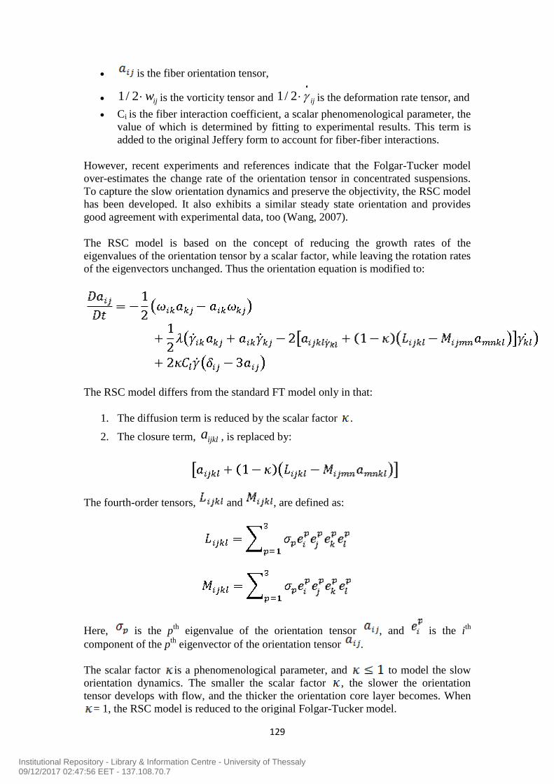
129

is the fiber orientation tensor,

1/ 2 ijw is the vorticity tensor and 1/ 2 ij is the deformation rate tensor, and

Ci is the fiber interaction coefficient, a scalar phenomenological parameter, the

value of which is determined by fitting to experimental results. This term is

added to the original Jeffery form to account for fiber-fiber interactions.

However, recent experiments and references indicate that the Folgar-Tucker model

over-estimates the change rate of the orientation tensor in concentrated suspensions.

To capture the slow orientation dynamics and preserve the objectivity, the RSC model

has been developed. It also exhibits a similar steady state orientation and provides

good agreement with experimental data, too (Wang, 2007).

The RSC model is based on the concept of reducing the growth rates of the

eigenvalues of the orientation tensor by a scalar factor, while leaving the rotation rates

of the eigenvectors unchanged. Thus the orientation equation is modified to:

The RSC model differs from the standard FT model only in that:

1. The diffusion term is reduced by the scalar factor .

2. The closure term, ijkla , is replaced by:

The fourth-order tensors, and , are defined as:

Here, is the pth

eigenvalue of the orientation tensor , and is the ith

component of the pth

eigenvector of the orientation tensor .

The scalar factor is a phenomenological parameter, and to model the slow

orientation dynamics. The smaller the scalar factor , the slower the orientation

tensor develops with flow, and the thicker the orientation core layer becomes. When

= 1, the RSC model is reduced to the original Folgar-Tucker model.


130

6. Results

Polymer fill region (3D):

The ‘polymer fill region’ result is generated at the end of filling and shows which

elements in the model are filled with polymer melt, at intervals as the cavity fills.

Filled elements are shown as green and unfilled elements as transparent. The polymer

fill region result is able to show where jetting flow has occurred. This effect is not

visible in the ‘fill time’ result, because it can show only one time (the first) that a node

fills. Figures 6.1-6.4 show the way the hot polymer fills the cavity at various times,

during the filling stage. Note that an even filling pattern exists and that filling is

uniform, too.

Note: Jetting occurs when polymer melt is pushed at a high velocity through

restrictive areas, such as the nozzle, runner, or gate, into open, thicker areas, without

forming contact with the mold walls. The buckled, snake-like jetting stream causes

contact points to form between the folds of melt in the jet, creating small-scale

"welds". Generally, jetting may result in uneven filling and may lead to air traps

inside the part. It can also lead to uneven cooling and increased stress in the part.

Jetting leads to part weakness, surface blemishes and a multiplicity of internal defects.

Figure 6.1: Polymer fill region at 0.2 sec. Figure 6.2: Polymer fill region at 0.5 sec.

Figure 6.3: Polymer fill region at 0.8 sec. Figure 6.4: Polymer fill region at 1 sec.


131

Fill time (3D):

The disk (cavity) is completely filled at 1.03 sec. The material is injected from the top

of the sprue, with a constant flow rate of 28 cm3/sec. Thus, it is expected for the

regions near the base of the sprue to fill first and for the regions far from the center

(edges) to fill last, as shown in figure 6.5

Figure 6.5: Predicted filling times for the disk cavity. (Scale range: 0 – 1.031 sec).

Average velocity (Dual Domain):

The ‘average velocity’ result shows the gap-averaged magnitude of velocity of the

polymer melt, inside the mold cavity, over time. This magnitude of the flow velocity

is an average through the thickness, calculated only in the regions where melt still

exists; the frozen layers are not included in this calculation.

The average velocity results at four different times of the filling stage are depicted in

figures 6.6-6.9. The anticipated unidirectional and uniform flow is observed (radial

direction). The flow does not reverse on itself, during the filling phase and no

hesitation flow (when the flow slows down or stops along a particular flow path) or

weld regions exist.

The highest velocity values are observed inside the sprue. More specifically, higher

values will appear on the top of the sprue and lower where it meets the part. This is

because material travels from a narrow cross-section to a wider one.

According to reports, for the geometry of a center-gated disk, if the fluid fills the

cavity at a constant flow rate, the flow decelerates with increasing radial distance.


132

As the material exits the sprue and enters the cavity, moving in a uniform fashion in

the radial direction, the area available to flow decreases, i.e. Q = A(r)*V(r), with:

A(r) = 2*pi*r*h, where h is the thickness of the mold and V(r) the velocity (radial) at

position (r). Since the volumetric flow rate (Q) is constant – filling occurs under

constant ram displacement – V(r) is inversely proportional to the radial distance (r).

Therefore, a series of plots are also presented (figures 6.10-6.15), depicting the

average velocity as a function of distance from the gate, in the radius direction, i.e.

V(r). In total, 18 random points were selected across the radius. At t = 0.53 sec (figure

6.10), the melt has almost reached the 40 mm distance. At r = 0, the maximum

velocity is observed (113 cm/s) and at a location 4 mm ahead, the velocity has already

dropped down to 40 cm/s. Just after mold filling has been completed (figure 6.13), a

small extra amount of material flows into the cavity, due to the packing pressure.

Moreover, the observed velocity at the injection location is much smaller (7.5 cm/s).

As we reach the end of packing (figure 6.15), flow into the cavity becomes zero.

The equations described above apply to an incompressible flow. In our case, that is

the filling phase. But does this equation ( ( )2

QV r

rh ) give results that are close to

the ones acquired from Moldflow? Let’s pick the 0.34 and 0.53 sec time points, where

the flow rate is constant and measured at 27.89 cm3/sec and 27.91 cm

3/sec,

respectively. Because the first point selected was for r = 0, the above equation gives

an infinite V(r). For this reason, as shown in figures 6.16 and 6.17, the first velocity

value on the “blue” curve is around 445 cm/s. The specific value was acquired by

using a very small radius distance, i.e. r = 0.5 mm. This was done just to present the

velocity difference that exists at r = 0 in a better way.

According to figures 6.16 and 6.17, the velocity values start converging for r 15

mm. Before that, the velocity difference is noticeable and the closer to r = 0 – the

greater the difference. Indicatively (equation vs. Moldflow results):

At r = 4 mm: 54.56 cm/s vs. 39.6 cm/s, at t = 0.34 sec and 54.2 cm/s vs. 39

cm/s, at = 0.53 sec.

At r = 7.8 mm: 28.21 cm/s vs. 23.4 cm/s, at t = 0.34 sec and 28.2 cm/s vs. 22.8


At r = 15 mm: 14.5 cm/s vs. 13.6 cm/s, at t = 0.34 sec and 14.6 cm/s vs. 13.3

cm/s, at t = 0.53 sec.

At r = 19 mm: 11.6 cm/s vs. 11.3 cm/s, at t = 0.34 sec and 11.7 cm/s vs. 11.1


At r = 28.3 mm: 7.85 cm/s vs. 8.18 cm/s, at = 0.34 sec and 7.8 cm/s vs. 7.5

cm/s, at t = 0.53 sec.

Possible explanations:

a) Deviation of the velocity profile predicted by Moldflow from the 1-D model

assumed by the equation.

b) Deviation from the incompressible flow assumed by the equation.


133

c) Based on the assumption that a dual-domain analysis probably uses the

General Hele-Shaw (GHS) methodology for the cavity filling and considering

that the GHS model is valid at some distance from the gate, indeed, this

deviation should be expected.

Figure 6.6: Average velocity at 0.24 sec. Figure 6.7: Average velocity at 0.53 sec.

(Scale range: 0 – 376.2 cm/s). (Scale range: 0 – 376.2 cm/s).

Figure 6.8: Average velocity at 0.82 sec. Figure 6.9: Average velocity at 1 sec.

(Scale range: 0 – 376.2 cm/s). (Scale range: 0 – 376.2 cm/s).


134

Figure 6.10: Velocity (cm/s) vs. distance from the gate (mm), at t = 0.53 sec (left).

Figure 6.11: Velocity (cm/s) vs. distance from the gate (mm), at t = 0.82 sec (right).

Figure 6.12: Velocity (cm/s) vs. distance from the gate (mm), at end of filling (left).


Figure 6.14: Velocity (cm/s) vs. distance from the gate (mm), at t = 2.2 sec (left).



135

Figure 6.16: Velocity (cm/s) vs. radial distance (mm), at t = 0.34 sec. The “blue”

curve depicts the velocity results acquired from the equation and the “red” curve

depicts the velocity results given by Moldflow.

Figure 6.17: Velocity (cm/s) vs. radial distance (mm), at t = 0.53 sec. The “blue”

curve depicts the velocity results acquired from the equation and the “red” curve

depicts the velocity results given by Moldflow.


136

Orientation at core & orientation at skin (Dual Domain):

The ‘orientation at skin’ result provides a good indication of how molecules or fibers

(when using a fiber-filled material) will be oriented on the outside of the part,

showing the average principal alignment direction for the whole local area at the end

of filling. The ‘orientation at core’ result provides a good indication of how molecules

or fibers will be oriented at the part core, showing the average principal alignment

direction for the whole element.

According to reports, in a center-gated disk (CGD) the fibers are transversely aligned

at core and flow aligned at skin. The main flow direction in a CGD is radial. Indeed,

figures 6.18 and 6.19 verify the theory.

Figure 6.18:

The orientation at

core result.

Figure 6.19:

The orientation at

skin result.


137

Pressure at injection location & Clamp force - XY Plot (3D):

The ‘pressure at injection location’ result (Pinjection) shows the pressure at the injection

location at various times, during the filling and packing phases of the analysis.

Actually it creates a XY plot of pressure vs. time, according to the results in the logs

dialog. This result is very useful for checking whether there are any pressure spikes,

which is normally a sign of imbalance.

The ‘clamp force’ result (Fclamp) is a time-series result which shows the force of the

mold clamp over time. The clamp force is the resultant value of the pressure

distribution over the entire part. It is a history of the force, resultant from filling and

packing pressure, which acts to open the mold.

Things should be made clear here. The Pinjection plot shows the pressure that a user

demands to be imposed on the top of the sprue (in the case of the CGD). The Fclamp

plot will actually show to a user how the system responds to this applied pressure. It’s

like observing how the cavity pressure develops over time.

In figure 6.20, one can see how the pressure gradually increases during the filling

phase. Right after this, the packing phase begins. Initially, it goes up to nearly 40 MPa

and for the next 4 sec the pressure remains constant at 50 MPa (end of packing). After

the packing phase is over, the pressure is released, reading the IMM for the next

cycle.

According to figure 6.21, the clamp force starts increasing and reaches the 27 tonnes

at the end of fill (1 sec). Its peak is observed around 1.5 sec (61.6 tonnes). After the

1.68 sec time, clamp force starts dropping, as the frozen volume of the material in the

cavity takes up more and more place (> 40%).

For both cases the time axis has been set to end at 6 sec. The reason was that after the

5.2 sec time both clamp force and injection pressure have dropped to 0. Thus, setting

the x axis to 6 sec gives a better presentation of the plot. The total cycle time is 11 sec

(15 sec if the mold-open time is also considered).

Note: A polymer is considered to be frozen, when the temperature falls below the

transition temperature (Ttrans). For our case: Ttrans. = 201 oC.


138

Figure 6.20: Pressure at the injection location (MPa) vs. time (sec).

Figure 6.21: Clamping force (tonnes) vs. time (sec).


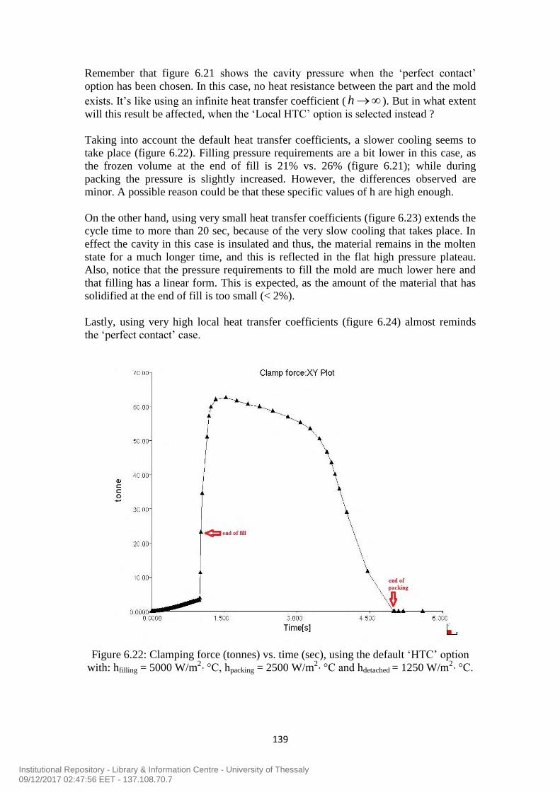
139

Remember that figure 6.21 shows the cavity pressure when the ‘perfect contact’

option has been chosen. In this case, no heat resistance between the part and the mold

exists. It’s like using an infinite heat transfer coefficient ( h ). But in what extent

will this result be affected, when the ‘Local HTC’ option is selected instead ?

Taking into account the default heat transfer coefficients, a slower cooling seems to

take place (figure 6.22). Filling pressure requirements are a bit lower in this case, as

the frozen volume at the end of fill is 21% vs. 26% (figure 6.21); while during

packing the pressure is slightly increased. However, the differences observed are

minor. A possible reason could be that these specific values of h are high enough.

On the other hand, using very small heat transfer coefficients (figure 6.23) extends the

cycle time to more than 20 sec, because of the very slow cooling that takes place. In

effect the cavity in this case is insulated and thus, the material remains in the molten

state for a much longer time, and this is reflected in the flat high pressure plateau.

Also, notice that the pressure requirements to fill the mold are much lower here and

that filling has a linear form. This is expected, as the amount of the material that has

solidified at the end of fill is too small (< 2%).

Lastly, using very high local heat transfer coefficients (figure 6.24) almost reminds

the ‘perfect contact’ case.

Figure 6.22: Clamping force (tonnes) vs. time (sec), using the default ‘HTC’ option

with: hfilling = 5000 W/m2 °C, hpacking = 2500 W/m

2 °C and hdetached = 1250 W/m2 °C.


140

Figure 6.23: Clamping force (tonnes) vs. time (sec), using the ‘HTC’ option with:

hfilling = 500 W/m2 °C, hpacking = 250 W/m


Figure 6.24: Clamping force (tonnes) vs. time (sec), using the ‘HTC’ option with:

hfilling = 50000 W/m2 °C, hpacking = 25000 W/m



141

Temperature (3D):

The ‘temperature’ result shows the temperature of the polymer at nodes, at specified

times during the analysis. The following figures show the temperature of the material,

through the part thickness, at specified times and for this reason the YZ cutting plane

has been selected. The times are: 1 sec (end of filling), 2.5 sec (packing phase), 5 sec

(end of packing) and 11 sec (end of cycle).

Figures 6.25-6.28 have something in common. Notice that every time the temperature

near the mold walls is much lower than that in the midplane of the cavity. This is

because of heat transfer between the hot molten plastic and the cold cavity walls.

At the end of filling (figure 6.25), the temperature in the midplane of the cavity is

around 258 °C. The closer to the surface - the smaller the temperature. At t = 2.5 sec,

it is obvious that temperature has decreased and the surface solidified layers have

grown more. At this point, the frozen volume is almost 60%. Notice how the green

color has taken up more space in the cavity (thickness direction). It is also obvious

that temperature at the center-plane is still high. At this time point, hot molten

material is still injected through the sprue (gate has not frozen yet).

At the end of packing (figure 6.27), the temperature at the midplane has decreased to

around 201 °C. The frozen volume is almost 100% and the cavity pressure has

dropped to zero. Where the cavity walls touch with the plastic, the material’s

temperature has become equal to the mold surface temperature (80 °C). Also, notice

the growth of the surface solidified layers, compared to the two figures before.

Note: Remember that Ttrans. = 201 °C. The moment packing phase ends, the frozen

volume is at 99.9%. This means that there is still a 0.1% portion in the cavity, where

the polymer has not yet turned to solid. Indeed, examining the region under the sprue,

gives temperatures both below 201 °C (solid state) and > 201 °C (melt state), i.e.

around 202-205 °C.

When the cycle time ends (figure 6.28), both injection and cavity pressure are zero.

The frozen layers have taken up most of the cavity space (blue color is dominating)

and the temperature at the midplane has dropped down to 150 °C.


142

Figure 6.25: Temperature at 1 sec. Figure 6.26: Temperature at 2.5 sec.

(Scale range: 80 – 285.3 oC). (Scale range: 80 – 285.3

oC).

Figure 6.27: Temperature at 5 sec. Figure 6.28: Temperature at 11 sec.

(Scale range: 80 – 285.3 oC). (Scale range: 80 – 285.3

oC).

Weld lines:

A weld line is formed when separate melt fronts traveling in opposite directions meet.

A meld line occurs if two emerging melt fronts flow parallel to each other and create a

bond between them. Weld and meld lines can be caused by holes or inserts in the part,

multiple gates, or variable wall thickness where hesitation occurs.

The ‘weld lines’ result displays the angle of convergence as two flow fronts meet. The

presence of weld lines may indicate a structural weakness and/or a surface blemish.

The term “weld line” is often used to mean both weld and meld lines. The only

difference between them is the angle at which they are formed; weld lines form at

lower angles than meld lines. Weld lines can cause structural problems and make the

part visually unacceptable, but they are unavoidable when the flow front splits and

comes together around a hole, or if the part has multiple gates.


143

Weld and meld lines should be avoided, particularly weld lines in areas that require

strength or a smooth appearance.

According to figure 6.29, no weld lines appear on the part.

Pressure (3D):

The ‘pressure’ result shows the pressure distribution through the flow path inside the

mold at the time the result was written. At the very beginning of filling, the pressure is

zero throughout the mold. The pressure at a specific location starts to increase, only

after the melt front reaches that location. The pressure continues to increase as the

melt front moves past, due to the increasing flow length between this specific location

and the melt front. The pressure difference from one location to another is the force

that pushes the polymer melt to flow, during filling. The pressure gradient is the

pressure difference divided by the distance between two locations.

A polymer always moves in the direction of the negative pressure gradient, i.e. from

higher pressure to lower pressure. Therefore, the maximum pressure occurs at the

polymer injection locations and the minimum pressure occurs at the melt front, during

the filling stage.

Through the ‘Clamp force: XY Plot’ result described earlier, the pressure inside the

cavity could also be examined. However, the goal here is to check how the cavity

pressure changes over time, when a very low and very high mold temperature is used.

Moreover, a series of plots will be presented, depicting the pressure as a function of

distance from the gate in the radius direction, i.e. P(r). In total 10 random points were

selected across the radius, with the node right at the center of the disk (R = 0) as the

starting point and with the node at the end (R = 65 mm) as the ending point.

Figure 6.29:

The weld lines result.


144

Figure 6.30: Clamping force (tonnes) vs. time (sec), for Tmold = 40

oC.

Figure 6.31: Clamping force (tonnes) vs. time (sec), for Tmold = 120

oC.


145

According to AMI logs, using the 40 oC as a constant mold temperature, gives a total

cycle time of 8.72 sec, while using the 120 oC gives a cycle time of 15.31 sec.

Therefore, a lower mold temperature decreases the cooling phase time, while a higher

mold temperature makes the cooling slower, i.e. cooling phase lasts longer.

As far as cavity pressure is concerned, it almost becomes zero at 4.1 sec (figure 6.30),

while 2 more seconds are needed in the second case (figure 6.31). Thus, a lower mold

temperature forces the pressure to drop to zero much faster. Also, notice the

difference at the filling phase. A more sudden increase takes place in the first case,

while in the second case filling seems to have a more linear form. Colder molds are

more difficult to fill, necessitating higher injection pressure (41 MPa vs. 34 MPa).

Because of the very low mold temperature, material has cooled faster; viscosity is

higher, so the pressure requirements are higher, too.

Moreover, one can tell that after t = 1.5 sec, the curve is much steeper in figure 6.30.

Something that does not happen in the other case. The reason is that a high mold

temperature causes the frozen volume to develop much slower. For example, at t = 3

sec, the frozen volume for Tmold = 40 oC is about 98%, while for Tmold = 120

oC it is

only 54%.

Lastly, figures 6.32-6.35 show the cavity pressure behavior as the flow front moves

further from the sprue gate. During the filling phase, the further from the gate – the

lower the pressure. It is also observed that average pressure increases during the

packing phase (figure 6.33), as expected. Towards the end of packing (figure 6.34),

average pressure inside the cavity has dropped, as the frozen volume has taken up

most of the space (~ 99%). At the end of packing and till the cycle time ends, cavity

pressure has dropped to zero and remains zero, as shown in figure 6.35.

Figure 6.32: Pressure (MPa) vs. distance from the gate (mm), at t = 1 sec.


146

Figure 6.33: Pressure (MPa) vs. distance from the gate (mm), at t = 2.5 sec.



147


Pressure at end of fill & Pressure at V/P switchover (3D):

The ‘pressure at end of fill’ result shows the pressure distribution in the cavity

at the instant, when the cavity is completely filled with polymer.

As one can notice from figure 6.36 below, the pressure distribution is uniform. The

maximum pressure (37 MPa) is located at the top of the sprue, where the hot material

is directly injected into the sprue and the lowest pressure is observed at the disk walls

(18-19 MPa).

The ‘pressure at V/P switchover’ result shows the pressure distribution

through the flow path inside the mold at the switchover point from velocity to

pressure control.

Remember that the switch-over from velocity to pressure control was set to happen,

when 98% of the cavity was filled. According to AMI logs, this happened exactly

when 98.1% of the disk was filled. At that moment, the time was 0.99 sec and the

injection pressure at 33.7 MPa. The red circle, on figure 6.37, simply indicates the 2%

of cavity’s volume that was unfilled.


148

Figure 6.36: Pressure at the end of fill (t = 1 sec). (Scale range: 18.30 – 37.03 MPa).

Figure 6.37: Pressure at the V/P switchover. (Scale range: 0 – 33.75 MPa).


149

Temperature at flow front (Dual domain & 3D):

The ‘temperature at flow front’ result shows the temperature of the polymer, when the

flow front reaches a specified point in the center of the plastic cross-section. The flow

front temperatures should not drop more than 2-5 oC, during the filling phase.

Figure 6.38: Temperature at flow front (Dual Domain).

(Scale range: 249.1 – 251.3 oC).

Figure 6.39: Temperature at flow front (3D).

(Scale range: 248.3 – 259.5 oC).


150

A rise in the melt front temperature is observed, as the melt front travels away from

the gate. This appears counter-intuitive, but can only be explained as a result of

viscous dissipation within the still molten material. This heat is transferred through

conduction to the mold walls and convected with the melt. However, conduction is

known to be very low in polymers, due to their poor thermal conductivity. As a result,

viscous heat produced is convected downstream with the melt and results in the melt

front having a slightly increasing temperature, as it travels downstream into the

cavity. According to figure 6.38, no temperature variations > 2 o

C exist. However,

what is interesting enough here, is the fact that the 3D result (figure 6.39) gives a 10

oC temperature variation for the disk.

Density (3D):

The ‘density’ result shows the density of the tetrahedral elements before shrinkage

occurs, at the time the result file was written. The program measures the density of the

material at this time and uses it as the starting point for calculation of the volumetric

shrinkage and warpage of the part. The figures below show the material’s density

through the part thickness at specified times and for this reason the YZ cutting plane

has been selected. The times are: 1 sec (end of filling), 2.5 sec (packing phase), 5 sec

(end of packing) and 11 sec (end of cycle).

This result determines whether the part was uniformly packed with polymer, during

the packing phase. Variations in polymer density can indicate problems with the part.

Once the material has filled the mold cavity and the packing phase has begun,

material flow is driven by the variation of density across the part. If one region of a

part is less densely packed than an adjacent region, then polymer will flow into the

less dense region, until equilibrium is reached.

Figures 6.40-6.43 have something in common. Notice that every time the density near

the mold walls is much higher than that in the midplane of the cavity. It has been

already mentioned that the polymer’s density behavior is described through the pvT

model, where density is dependent both on pressure and temperature (ρ(T,P)). As

pressure increases, so does the density. Also, the more temperature decreases - the

more density increases. So which of those two variants affects the density result

more?

Having tested manually the effect of both parameters into equations 4.1.4.1 and

4.1.4.2, i.e. the 0-50 MPa pressure range and the 80-250 oC temperature range, it was

eventually concluded that temperature has the biggest impact on density. This is

possibly explained by the fact that the material is semi-crystalline.

At the end of filling (figure 6.40), the density of the polymer in the midplane is 1.29

g/cm3. The closer to the surface - the higher the density. At t = 2.5 sec (packing

phase), the cavity pressure has already begun to drop. Thus, one would expect for the

density to drop, as well. According to figure 6.41, this is not true. And the reason is

temperature. At this point, temperature at the cavity walls has dropped down to almost

80 o

C. Therefore, it is expected for the density to have nearly reached its max value.

Indeed, at the wall surface a value of 1.48 g/cm3 is observed, while in the midplane

this value is much smaller, at 1.31 g/cm3.


151

The more we reach the end of cycle, the more temperature is decreased. Therefore, it

is expected for the density in the midplane to increase more and more. Indeed, notice

how the light blue color has vanished in the cavity (figure 6.42). It is also obvious that

the disk has been uniformly packed with polymer and no variations exist. At the

cavity walls, density has already reached its max value (1.484 g/cm3) and in the

midplane its value is 1.37 g/cm3, at the end of packing phase (figure 6.42) and 1.42

g/cm3, when the molding cycle has ended (figure 6.43).

Figure 6.40: Density at t = 1 sec. Figure 6.41: Density at t = 2.5 sec.

(Scale range: 1.258 – 1.484 g/cm3). (Scale range: 1.258 – 1.484 g/cm

3).

Figure 6.42: Density at t = 5 sec. Figure 6.43: Density at t = 11 sec.

(Scale range: 1.258 – 1.484 g/cm3). (Scale range: 1.258 – 1.484 g/cm

3).


152

Average volumetric shrinkage (3D):

The ‘Average volumetric shrinkage’ result shows the average value of volumetric

shrinkage over the half-gap thickness for 3D models.

Volumetric shrinkage is the percentage increase in local density from the end of the

filling-packing phase to when the part has cooled to the ambient temperature (23°C).

The calculations begin once the cavity is filled, based on the difference between the

current pvT state and the reference state:

where:

VS is the volumetric shrinkage,

AD is the average density,

D is the density, and

the pressure p is zero and temperature T is the specified ambient temperature.

As the mass of an element changes (for example, with polymer flow during packing),

shrinkage continues to change with each change in the element's pvT state. Once the

mass stops changing, the element's current pvT state is fixed in the shrinkage

calculation, as the reference state. The average volumetric shrinkage of the part is

depicted below, at four different times: t = 1.5 sec (slightly after filling has ended), t =

2.7 sec & t = 3.5 sec (packing phase) and t = 5 sec (end of packing).

Figure 6.44: Average shrinkage at 1.5 sec. Figure 6.45: Average shrinkage at 2.7 sec.

(Scale range: 3.986 – 12.34%). (Scale range: 3.986 – 12.34%).


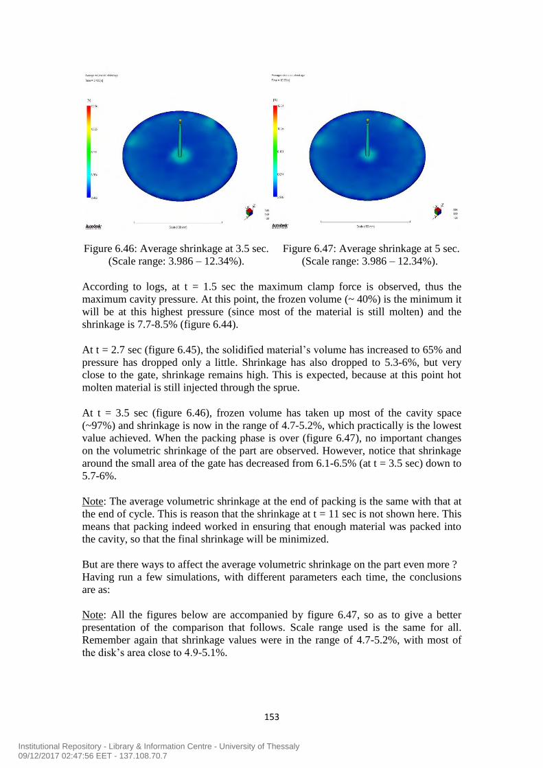
153

Figure 6.46: Average shrinkage at 3.5 sec. Figure 6.47: Average shrinkage at 5 sec.

(Scale range: 3.986 – 12.34%). (Scale range: 3.986 – 12.34%).

According to logs, at t = 1.5 sec the maximum clamp force is observed, thus the

maximum cavity pressure. At this point, the frozen volume (~ 40%) is the minimum it

will be at this highest pressure (since most of the material is still molten) and the

shrinkage is 7.7-8.5% (figure 6.44).

At t = 2.7 sec (figure 6.45), the solidified material’s volume has increased to 65% and

pressure has dropped only a little. Shrinkage has also dropped to 5.3-6%, but very

close to the gate, shrinkage remains high. This is expected, because at this point hot

molten material is still injected through the sprue.

At t = 3.5 sec (figure 6.46), frozen volume has taken up most of the cavity space

(~97%) and shrinkage is now in the range of 4.7-5.2%, which practically is the lowest

value achieved. When the packing phase is over (figure 6.47), no important changes

on the volumetric shrinkage of the part are observed. However, notice that shrinkage

around the small area of the gate has decreased from 6.1-6.5% (at t = 3.5 sec) down to

5.7-6%.

Note: The average volumetric shrinkage at the end of packing is the same with that at

the end of cycle. This is reason that the shrinkage at t = 11 sec is not shown here. This

means that packing indeed worked in ensuring that enough material was packed into

the cavity, so that the final shrinkage will be minimized.

But are there ways to affect the average volumetric shrinkage on the part even more ?

Having run a few simulations, with different parameters each time, the conclusions

are as:

Note: All the figures below are accompanied by figure 6.47, so as to give a better

presentation of the comparison that follows. Scale range used is the same for all.

Remember again that shrinkage values were in the range of 4.7-5.2%, with most of

the disk’s area close to 4.9-5.1%.


154

a) The higher the pressure used in the packing/holding profile – the more

shrinkage is reduced. Pressure affects directly the density (or specific volume),

therefore the shrinkage. However, don’t forget that there is always the

clamping force limitation of the IMM. Increasing the packing pressure by 20

MPa drops the shrinkage down to 4.1-4.7%. Most of the disk’s area has a

shrinkage close to 4.2-4.3% (figure 6.49).

Figure 6.48: Average volumetric shrinkage at the end of cycle.

(Scale range: 3.986 – 6.5%).

Figure 6.49: Average volumetric shrinkage at the end of cycle, for Ppacking = 70 MPa.

(Scale range: 3.446 – 6.5%).

b) The lower the mold temperature – the lower the volumetric shrinkage. Using a

mold temperature of 60 oC drops the shrinkage down to 4.2-4.8%. Most of the

disk’s area has a shrinkage close to 4.6-4.8% (figure 6.51). Injecting the semi-

crystalline PBT into a colder mould, causes a more rapid cooling, which slows

down the formation of crystalline areas, resulting in a lower shrinkage.


155


(Scale range: 3.986 – 6.5%).

Figure 6.51: Average volumetric shrinkage at the end of cycle, for Tmold = 60 oC.

(Scale range: 3.477 – 6.5%).

c) The slower the cavity fills – the lower the volumetric shrinkage. Setting a flow

rate of 11.5 cm3/sec, increases the filling time to 2.55 sec. At the start of

packing phase, a larger percent of the material has solidified, namely 43%

(figure 6.53) vs. 26% (figure 6.52). A slower filling causes the frozen layers to

become thicker. As a result, the actual flow channel for the material gets

smaller. Therefore, more pressure is required to fill the mold and the in-cavity

pressure values will be higher, resulting in a lower shrinkage. It is obvious

how the blue color is dominating in figure 6.53. The range of shrinkage values

is 4.5-5.1%, with most of the disk’s area around 4.6-4.8%.


156


(Scale range: 3.986 – 6.5%).

Figure 6.53: Average volumetric shrinkage at the end of cycle, for an injection time of

2.5 sec. (Scale range: 4.04 – 6.5%).

d) Using very small heat transfer coefficients (HTC) seems to have a big impact

on shrinkage, too. However, volumetric shrinkage is not reduced, but

increased to 8.1-8.3%. This is expected, as in this case cooling is very slow;

namely, ~ 25% frozen volume (figure 6.55) vs. 99% (figure 6.54), at t = 4.5

sec. The scale here was set to 9%, as the minimum shrinkage value was 6.5%

(figure 6.55). A very slow cooling means that it will take longer for the part to

freeze, which makes the crystalline content increase. Therefore, the resulting

shrinkage is much higher.


157


(Scale range: 3.986 – 6.5%).

Figure 6.55: Average volumetric shrinkage at the end of cycle, using the ‘HTC’

option with: hfilling = 500 W/m2 °C, hpacking = 250 W/m

2 °C and hdetached = 125 W/m2

°C. (Scale range: 6.587 – 9%).

e) Increasing the melt temperature may increase or decrease shrinkage.

Typically, very low melt temperatures lead to relatively high shrinkage,

because the part cannot be adequately packed out. Increasing the temperature,

up to a certain point, decreases the shrinkage because viscosity is reduced and

so packing pressure can be better distributed through the cavity. For a given

packing pressure and time, further increase in melt temperature leads to higher

shrinkages, as the cavity is then filled with material of relatively low density

(Shoemaker J., 2006). The main difference, between figures 6.56 and 6.57, is

the area around the gate.


158

Using hotter material causes the shrinkage near the sprue to increase from

about 5.9% to 6.4%. Volumetric shrinkage in the rest of the disk remains

pretty much the same (4.8-5.2%).


(Scale range: 3.986 – 6.5%).

Figure 6.57: Volumetric shrinkage at the end of cycle, for Tmelt = 270 oC.

(Scale range: 3.961 – 6.5%).

Note: Another parameter that can affect volumetric shrinkage is the gate diameter.

The shrinkage of a moulding can be reduced by enlarging the gate, so as to increase

feeding (Mills N., 2005).


159

Volumetric Shrinkage (3D) & Density (3D) results comparison:

The ‘Volumetric shrinkage’ result shows the volumetric shrinkage for each node, as a

percentage of the original volume. Here, five figures of density and shrinkage

behavior will be presented at different times of the molding cycle, right at the center-

plane of the disk, i.e. (x, y, z) = (0, 0, 1).

Volumetric shrinkage calculations begin once the cavity is filled, based on the

difference between the current pvT state and the reference state (where the pressure p

is zero and temperature T is the specified ambient temperature):

As the mass of an element changes (for example, with polymer flow during packing),

shrinkage continues to change with each change in the element's pvT state. Once the

mass stops changing, the element's current pvT state is fixed in the shrinkage

calculation as the reference state.

The mass of an element stops changing, when the cavity pressure has decayed to zero.

After this, the volumetric shrinkage becomes a constant ( ). However, if the holding

pressure is removed before the material is frozen or while the pressure in the cavity is

still non-zero, the volumetric shrinkage may rebound due to possible backflow into

the nozzle or other warmer areas of the part.

Figure 6.58: Density at t = 1.5 sec. Figure 6.59: Shrinkage at t = 1.5 sec.

(Scale range: 1.258 – 1.484 g/cm3). (Scale range: 1.601 – 13.43%).


160





Figure 6.64: Density at t = 5 sec. Figure 6.65: Shrinkage at t = 5 sec.



161

Figure 6.66: Density at t = 11 sec. Figure 6.67: Shrinkage at t = 11 sec.


At t = 1.5 sec, the maximum clamp has been observed, thus, the cavity pressure has

reached the maximum value (~ 46 MPa). Also, at this point, temperature is at about

254 oC. Density is at 1.31 g/cm

3 (higher than that at t = 1 sec (1.28 g/cm

3), as pressure

has increased; figure not presented here) and shrinkage measures at about 13%, i.e.

almost the maximum value it can have (figure 6.59).

As we move into the packing phase, at t = 2.7 sec, pressure has slightly dropped, but

temperature has been reduced to 220 oC. Therefore, it is expected for the density to

have increased (1.37 g/cm3). Some spatial shrinkage variations appear on figure 6.61,

however, on average the shrinkage has dropped to about 8.6 - 9.2%.

At t = 3.5 sec, pressure is around 38 MPa near the center of the disk, while far from it,

it does not exceed 28 MPa. Also, temperature is at about 205 oC. Testing the effect of

the two parameters into equations 4.1.4.1 and 4.1.4.2, proves again that temperature is

much more effective in increasing the density. Density has now increased to 1.39

g/cm3 and shrinkage has dropped to 7.3% (figures 6.62 and 6.63). Notice the high

shrinkage near the sprue (10.7-11.5%).

At the end of packing period (t = 5 sec), as we have already seen, shrinkage remains

more or less the same, and only near the sprue area a reduction is observed (8.8-

9.4%). Pressure has become zero (ambient) and temperature has reached 175 oC.

Density is increased a little, at 1.41 g/cm3. The shrinkage observed at t = 5 sec is also

the one observed in the final product.

At the end of cycle (t = 11 sec), density has increased even more (1.45 g/cm3).

However, from figure 6.67 it is clear that shrinkage has not changed at all. Normally,

a small shrinkage decrease would be expected near the sprue. The most possible

reason for this may be the fact that a packing time of 4 sec was used in the analysis.

This caused the cavity pressure to decay to zero, just at the end of packing period, i.e.

after this, shrinkage remains the same ( ). Remember that the part weight remained

constant after t = 3.5 sec. So now the time has been extended for 0.5 sec. This reminds

once again the importance of the time factor in injection molding.


162

The following figures (6.68 – 6.71) show the density and shrinkage results at the end

of packing/holding period and at the end of cycle, using tpacking = 3.5 sec. Indeed,

volumetric shrinkage is decreased at the center (close to the sprue) and covers a

smaller area. This probably reflects the fact that there is still a small flow of material

in that area.

Figure 6.68: Density at end of packing. Figure 6.69: Shrinkage at end of packing.

Figure 6.70: Density at end of cycle. Figure 6.71: Shrinkage at end of cycle.

Lastly, the following figures (6.72 - 6.76) show the volumetric shrinkage at the end of

cycle, for five different points in the thickness direction. Of course, the closer to the

surface - the lower the volumetric shrinkage.


163

Figure 6.76: Shrinkage at (x, y, z) =

(0, 0, 2). Values: 1.8 - 2%.


(0, 0, 1). Values: 7.2 - 7.5%.


(0, 0, 1.25). Values: 6.7 - 7%.


(0, 0, 1.5). Values: 5.4 - 5.8%.


(0, 0, 1.75). Values: 3.6 - 4%.


164

Suggestions for future studies

Effect of viscous heating on 3D temperature profiles.

Study of the fiber orientation tensor, using the Folgar-Tucker and the RSC

model.

Focus on the kinetics of crystallization and its effect on volumetric shrinkage.

Examine the volumetric shrinkage, of fiber-filled TPs, in the flow direction

and perpendicular to the flow direction.

REFERENCES

Baldwin J.D., Altan M.C. and Rajamani K. Structural Analysis of an Injection

Molded Short-Fiber-Reinforced Disk. Journal of Materials Processing &

Manufacturing Science, vol. 6, USA, October 1997.

Bay R.S. & Tucker III C.L. Fiber Orientation in Simple Injection Moldings.

Part I: Theory and Numerical Methods. Polymer Composites, vol. 13, p. 317-

331, Illinois, August 1992.

BASF Corporation Engineering Plastics. Estimating Cooling Times in

Injection Molding (2007).

Benretem A., Benidir M. and Chaib R. Factors Influencing Slurry Rheology.

WorldPumps, p. 30-31, July 2010.

Dantzig J.A. & Tucker III C.L. Modeling in Materials Processing (p. 218).

Cambridge University Press, 2001.

DSM Engineering Plastics. Performance and Value with Engineering Plastics

– Design Guide, USA, 2005.

DuPont Performance Polymers. Thermoplastic Polyester Resin - Crastin®

HR5330HF NC010, Product Information, 2013.

DuPontTM

Delrin acetal resin – Molding Guide (Technical Information), USA,

2006.

Engelmann Paul & Dealey Bob. Injection Molding Design Guidelines –

Maximizing Performance Using Copper Alloys. For the Mold Marketing Task

Group of the Copper Development Association, May, 1999.

Groover Mikell P. Fundamentals of Modern Manufacturing Materials,

Processes, and Systems (4th

edition). John Wiley & Sons, Inc. USA, 2010.

Islam A., Hansen H.N., Gasparin S. and Bondo M. Effects of Glass Fibers on

the Properties of Micro Molded Plastic Parts. Department of Mechanical

Engineering, Technical University of Denmark, 2011.


165

Jian Wang. PVT Properties of Polymers for Injection Molding - Some Critical

Issues for Injection Molding. School of Chemical Engineering and

Environment, Beijing Institute of Technology, China, 2012.

Kunc Vlastimil, Frame Barbara, Nguyen Ba Nghiep, Tucker III Charles L. and

Vélez-García Gregorio. Fiber Length Distribution Measurement for Long

Glass and Carbon Fiber Reinforced Injection Molded Thermoplastics (2007).

Mills Nigel. Plastics: Microstructure and Engineering Applications (Third

edition), p. 186. Butterworth-Heinemann, October 15, 2005.

Nguyen Quoc-Hung & Nguyen Ngoc-Diep. Incompressible Non-Newtonian

Fluid Flows, Continuum Mechanics - Progress in Fundamentals and

Engineering Applications, Dr. Yong Gan (Ed.), 2012.

O'Gara J. F., Wyzgoski M. G. and G. E. Novak. Development of an ISO

Standard for determining Anisotropic Properties of Glass-Filled

Thermoplastics. Proceedings of the 61th Annual Technical Conference and

Exhibition, May 4-8, 2003, Nashville, Tennessee, U.S.A.

Pontes A.J., Neves N.M. and Pouzada A.S. The role of the interaction

coefficient in the prediction of the fiber orientation in planar injection

moldings. Polymer Composites, vol. 24, p. 358-366. Department of Polymer

Engineering, Portugal, June 2003.

Rännar Lars-Erik. On optimization of Injection Molding Cooling. Norwegian

University of Science and Technology - Faculty of Engineering Science and

Technology. Department of Engineering Design and Materials. Trondheim,

April 2008.

Rosato Dominick V., Rosato Donald V. and Rosato Marlene G. Injection

Molding Handbook (3rd

edition). Kluwer Academic Publishers, USA, 2000.

Shoemaker Jay. Moldflow Design guide – A Resource for Plastics Engineers

(1st edition). Moldflow Corporation, Framingham, Massachusetts, USA, 2006.

Somjate Patcharaphun. Characterization and Simulation of Material

Distribution and Fiber Orientation in Sandwich Injection Molded Parts Faculty

of Mechanical Engineering, Institute of Mechanical and Plastics Engineering,

Chemnitz University of Technology, 2006.

Strong A. Brent. Plastics: Materials and Processing. Prentice Hall Inc., New

Jersey, 1996.

Tadmor Z. Molecular Orientation in Injection Molding. Journal of Applied

Polymer Science, vol. 18, p. 1753-1772, 1974.

Tadmor Z. & Gogos C. Principles of Polymer Processing, Wiley 1979.

Injection Molding of Polymers (14.1), p. 584 – 610.


166

Vélez-García Gregorio Manuel. Experimental Evaluation and Simulations of

Fiber Orientation in Injection Molding of Polymers Containing Short Glass

Fibers. Department of Macromolecular Science & Engineering, Virginia

Polytechnic Institute and State University, Blacksburg, USA, January 31,

2012.

Wang Jin & Jin Xiaoshi. Comparison of Recent Fiber Orientation Models in

AMI Simulations with Measured Fiber Orientation Data. Proceedings of the

polymer processing society 26th

annual meeting, Banff, Canada, July 4-8,

2010.

Wilkinson Arthur N. & Ryan Anthony J. Polymer Processing and Structure

Development (p. 233-234). Kluwer Academic Publishers, 1998.

ADDITIONAL LINKS

[Autodesk Moldflow Insight Help]:

http://wikihelp.autodesk.com/Simulation_Moldflow/enu/2013/Help/2.0Insight

[1]:

http://www.dc.engr.scu.edu/cmdoc/dg_doc/develop/material/overview/a3000001.htm

[2]: http://www.custompartnet.com/wu/InjectionMolding

[3]:

http://www.dc.engr.scu.edu/cmdoc/dg_doc/develop/process/physics/b3200002.htm

[4]:

http://megamould.com/TechBlog/Mold-

Design/Construction%20Injection%20Molds%20Classification.html

[5]: http://www.vnmold.com/2012/06/gate-designing-in-injection-mold-p1.html

[6]:

http://www.de.kuas.edu.tw/backup/laboratory/%E9%AB%98%E5%88%86%E5%AD

%90%E5%8A%A0%E5%B7%A5%E7%A0%94%E7%A9%B6%E5%AE%A4-

pplab/download/%E5%A1%91%E8%86%A0%E5%8A%A0%E5%B7%A5%E7%89

%B9%E8%AB%96-Chapter%202.4.4.pdf (page 52)

[7]: http://www.dc.engr.scu.edu/cmdoc/rm_doc/02_Material_props.html

[8]:

http://www.dc.engr.scu.edu/cmdoc/dg_doc/develop/process/control/b1000005.htm#21

6586

[9]: http://www.plastictroubleshooter.com/ThePlasticTroubleshooter/sink_marks.htm

[10]: http://www.dc.engr.scu.edu/cmdoc/rm_doc/04_Process_modeling.html


http://wikihelp.autodesk.com/Simulation_Moldflow/enu/2013/Help/2.0Insight

http://www.dc.engr.scu.edu/cmdoc/dg_doc/develop/material/overview/a3000001.htm

http://www.custompartnet.com/wu/InjectionMolding

http://www.dc.engr.scu.edu/cmdoc/dg_doc/develop/process/physics/b3200002.htm

http://megamould.com/TechBlog/Mold-Design/Construction%20Injection%20Molds%20Classification.html

http://megamould.com/TechBlog/Mold-Design/Construction%20Injection%20Molds%20Classification.html

http://www.vnmold.com/2012/06/gate-designing-in-injection-mold-p1.html

http://www.de.kuas.edu.tw/backup/laboratory/%E9%AB%98%E5%88%86%E5%AD%90%E5%8A%A0%E5%B7%A5%E7%A0%94%E7%A9%B6%E5%AE%A4-pplab/download/%E5%A1%91%E8%86%A0%E5%8A%A0%E5%B7%A5%E7%89%B9%E8%AB%96-Chapter%202.4.4.pdf




http://www.dc.engr.scu.edu/cmdoc/rm_doc/02_Material_props.html



http://www.plastictroubleshooter.com/ThePlasticTroubleshooter/sink_marks.htm

http://www.dc.engr.scu.edu/cmdoc/rm_doc/04_Process_modeling.html

computer aided design of an injection molded center-gated disc

Documents