computer-aided analysis of electronic circuits” course notes 3
TRANSCRIPT
Faculty of
Electronics, Telecommunications and Information
Technologies
Gheorghe Asachi Technical University of
Iasi
www.etti.tuiasi.rotuiasiC www.study.tuiasi.ro www.learning.tuiasi.ro
” Computer-Aided Analysis
of Electronic Circuits”
Course Notes 3
Lecturer: Dan Burdia, PhD
Bachelor: Telecommunication Technologies and Systems
Year of Study: 2

Contents
• I. Introduction in Computer-Aided Analysis.
•
• II. Computer Circuit Models of Electronic Devices and Components
• III. Network Topology: The Key to Computer Formulation of the
Kirchhoff Laws
• IV. Nodal Linear Network Analysis: Algorithms and Computational
Methods
• V. Nodal Nonlinear Resistive Network Analysis: Algorithms and
Computational Methods
2
Chapter III - Network Topology: The Key to Computer Formulation of the Kirchhoff Laws
• 3.1 Basic concepts in network topology
• 3.2 Incident matrix
• 3.3 Loops matrix
• 3.4 Cutset matrix
• 3.5 Basic relations between branch variables
• 3.6 Computer-aided formulation of A, B and D matrices
3
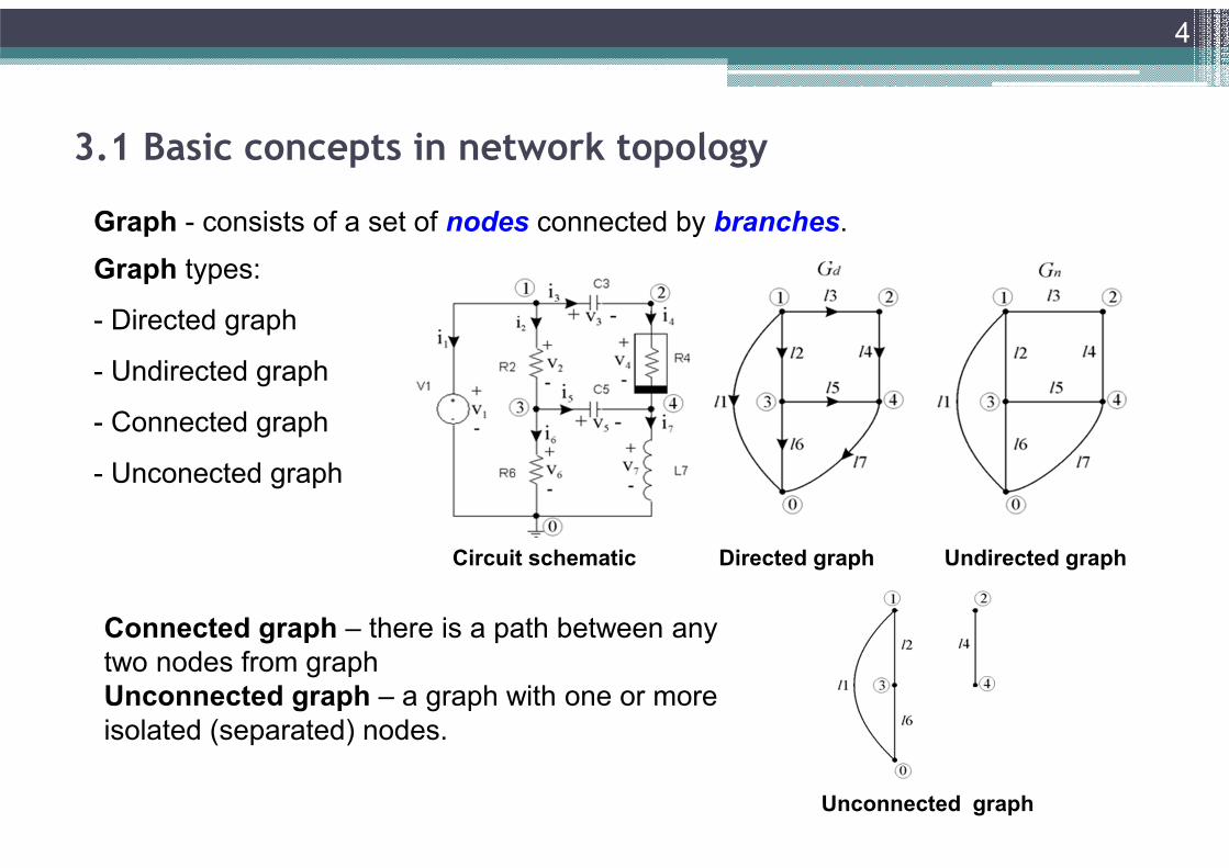
3.1 Basic concepts in network topology
4
Circuit schematic Directed graph Undirected graph
Graph - consists of a set of nodes connected by branches.
Graph types:
- Directed graph
- Undirected graph
- Connected graph
- Unconected graph
Connected graph – there is a path between any
two nodes from graph
Unconnected graph – a graph with one or more
isolated (separated) nodes.
Unconnected graph

• Loop
▫ A subgraph Gs of a graph Gn which fulfills the following two conditions:
� Gs is connected (connex)
� At each node in Gs there are exactly two branhes of the Gs
Example: 1,2,6; 1,3,4,5,6; 3,4,7,6,2; Not loop: 3,4,5,2,7
• Cut-set▫ A set of branches which fulfills the following two conditions:
� If the set is removed from graph then the graph becomes unconnected
� Re-inserting any branch from set the graph becomes again connected.
Example: 1,2,3; 3,5,7; 2,5,6; Not cutset: 3,2,5,7
• Tree
▫ A subgraph Gs of a graph Gn which fulfills the following three conditions:
� Gs is connected
� Gs contains all nodes from Gn
� Gn does not contain loops.
Example: 3,2,5,6; 3,4,6,7; Not tree: 1,2,6,5; 3,2,4,5,7
3.1 Basic concepts in network topology (cont)
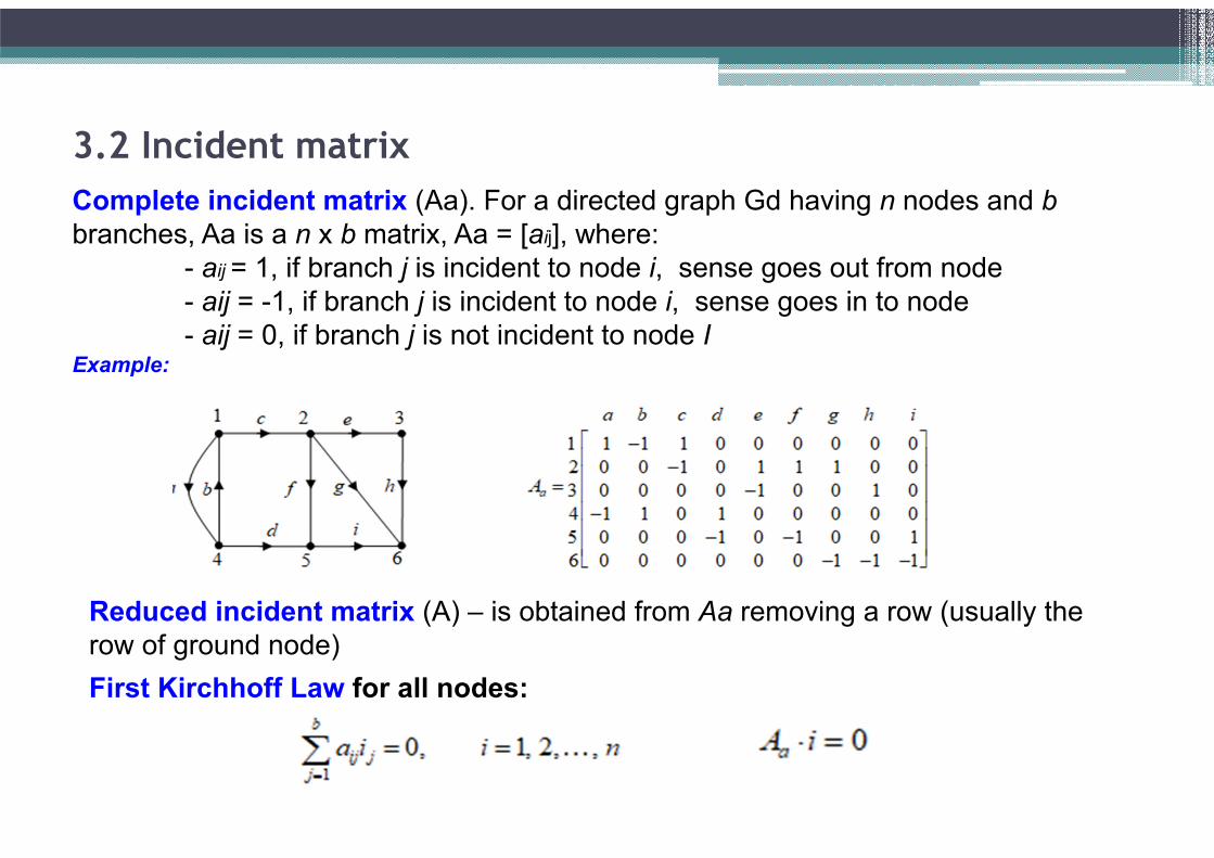
Complete incident matrix (Aa). For a directed graph Gd having n nodes and b
branches, Aa is a n x b matrix, Aa = [aij], where:
- aij = 1, if branch j is incident to node i, sense goes out from node
- aij = -1, if branch j is incident to node i, sense goes in to node
- aij = 0, if branch j is not incident to node IExample:
3.2 Incident matrix
Reduced incident matrix (A) – is obtained from Aa removing a row (usually the
row of ground node)
First Kirchhoff Law for all nodes:

3.2 Incident matrix (cont.)
Theorem 3.1. For a directed graph Gd the rows of reduced incident matrix A are
linear independent.
Corolar. The maximum set of independent First Kirchhoff Law equations are
written as: 0A i
Theorem 3.2. Given A the reduced incident matrix for a directed graph Gd having
n nodes. Then n-1 columns from A are linear independent if and only if the
branches corresponding to those columns form a tree in Gd.
Corolar. Let consider A partitioned as:
where AT and AL have the columns corresponding to the tree branches and co-tree
branches, respectively. Then det(AT) ≠ 0.
T LA A A M
Example:

3.3 Loops matrix
Definition. Complete loops matrix Ba
For a directed graph Gd with n nodes, b branches and nb directed loops,
Ba = [bij]nb x b, where:
bij= +1 if branch j belongs to the loop i, the same orientation
bij= -1 if branch j belongs to the loop i, the opposite orientation
bij= 0 if branch j does not belong to the loop i
Kirchhoff II Law for all possible loops (not all are independent):
Base loops matrix Bb: a submatrix of Ba having maximum independent rows from Ba
Bb have b-n+1 lines.
How we can select a set of b-n+1 independent rows (loops)?
Systematic approach: by determining the fundamental loops
Fundamental loop: contains only one branch from co-tree and the other
branches are from the tree. The loop orientation is the same to branch from co-tree.
Fundamental loops matrix B can be partitioned as B = [BT | 1]
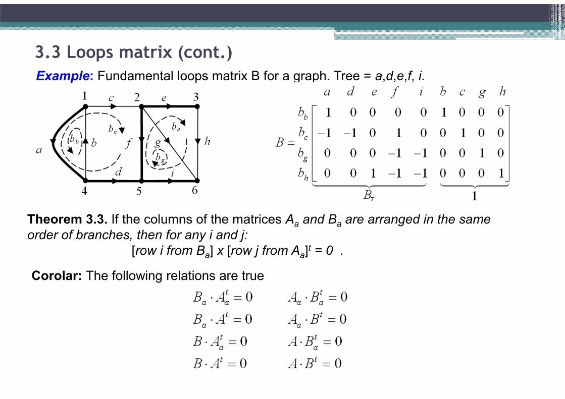
3.3 Loops matrix (cont.)
Example: Fundamental loops matrix B for a graph. Tree = a,d,e,f, i.
Theorem 3.3. If the columns of the matrices Aa and Ba are arranged in the same
order of branches, then for any i and j:
[row i from Ba] x [row j from Aa]t = 0 .
Corolar: The following relations are true
3.3 Loops matrix (cont.)
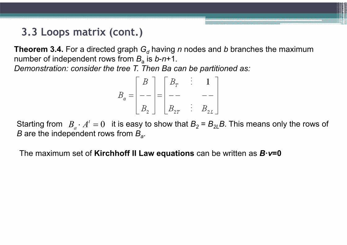
Theorem 3.4. For a directed graph Gd having n nodes and b branches the maximum
number of independent rows from Ba is b-n+1.
Demonstration: consider the tree T. Then Ba can be partitioned as:
Starting from it is easy to show that B2 = B2LB. This means only the rows of
B are the independent rows from Ba. 0t
aB A
The maximum set of Kirchhoff II Law equations can be written as B·v=0
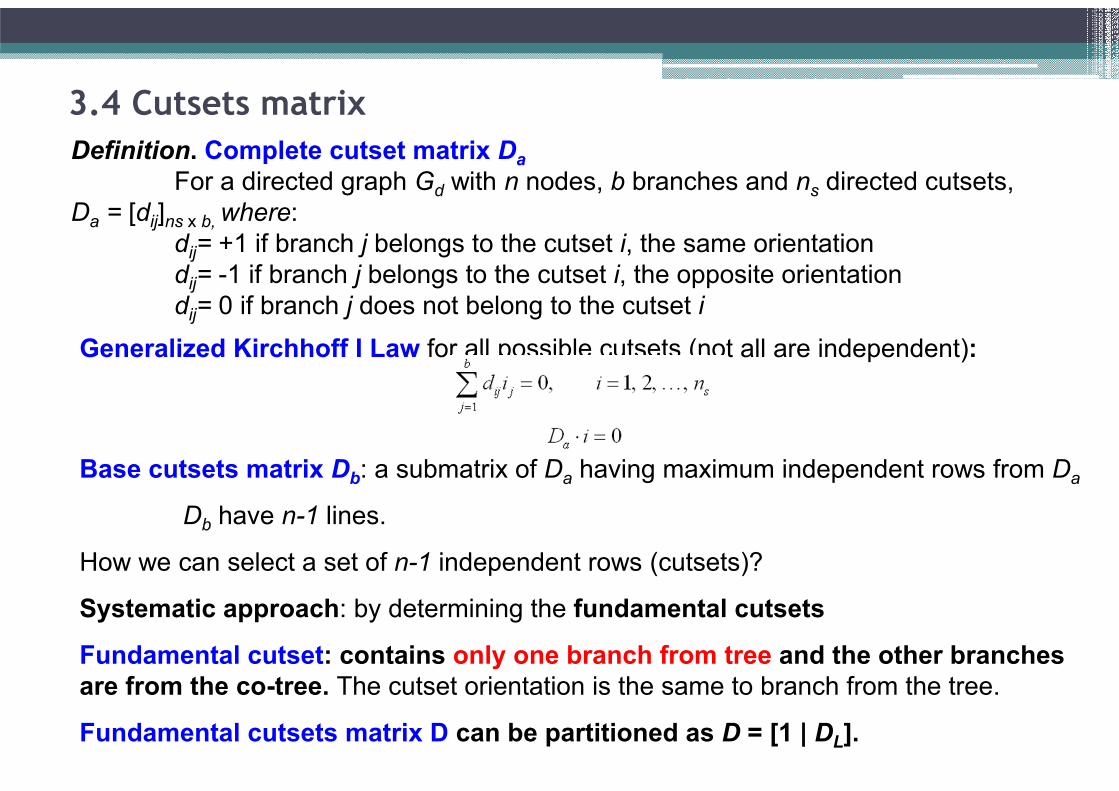
3.4 Cutsets matrix
Definition. Complete cutset matrix Da
For a directed graph Gd with n nodes, b branches and ns directed cutsets,
Da = [dij]ns x b, where:
dij= +1 if branch j belongs to the cutset i, the same orientation
dij= -1 if branch j belongs to the cutset i, the opposite orientation
dij= 0 if branch j does not belong to the cutset i
Generalized Kirchhoff I Law for all possible cutsets (not all are independent):
Base cutsets matrix Db: a submatrix of Da having maximum independent rows from Da
Db have n-1 lines.
How we can select a set of n-1 independent rows (cutsets)?
Systematic approach: by determining the fundamental cutsets
Fundamental cutset: contains only one branch from tree and the other branches
are from the co-tree. The cutset orientation is the same to branch from the tree.
Fundamental cutsets matrix D can be partitioned as D = [1 | DL].

3.4 Cutsets matrix (cont.)
Example 1. Complete cutset matrix Da
Example 2. Fundamental cutset matrix D for a graph. Tree T = a,d,e,f,i.
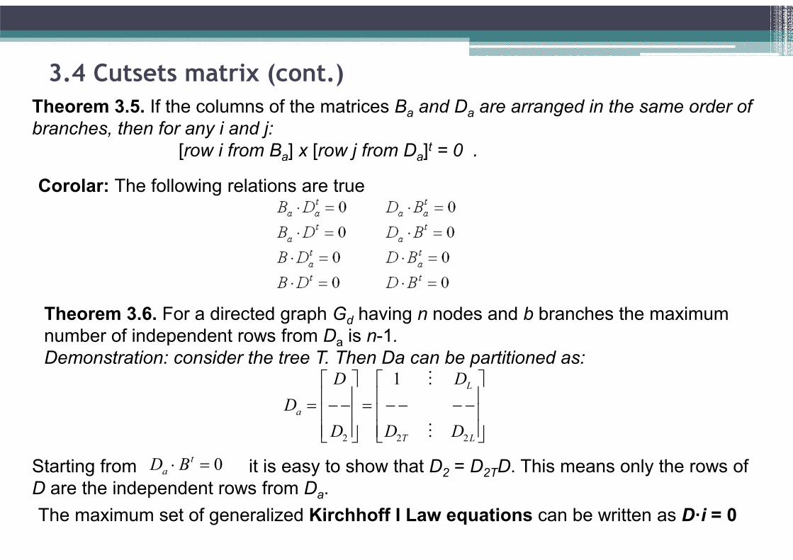
Theorem 3.5. If the columns of the matrices Ba and Da are arranged in the same order of
branches, then for any i and j:
[row i from Ba] x [row j from Da]t = 0 .
Corolar: The following relations are true
3.4 Cutsets matrix (cont.)
Theorem 3.6. For a directed graph Gd having n nodes and b branches the maximum
number of independent rows from Da is n-1.
Demonstration: consider the tree T. Then Da can be partitioned as:
2 2 2
1 L
a
T L
D D
D
D D D
M
M
0t
aD B Starting from it is easy to show that D2 = D2TD. This means only the rows of
D are the independent rows from Da.
The maximum set of generalized Kirchhoff I Law equations can be written as D·i = 0
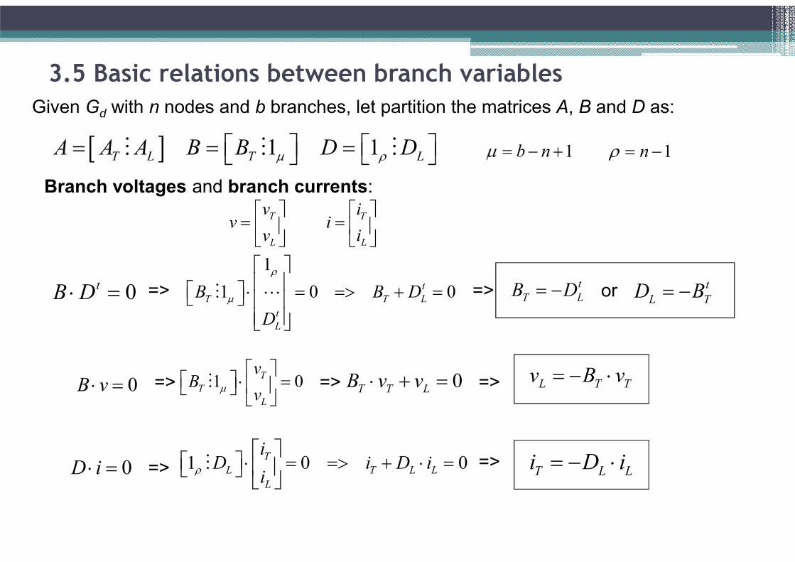
3.5 Basic relations between branch variables
Given Gd with n nodes and b branches, let partition the matrices A, B and D as:
1 1T L T LA A A B B D D M M M 1b n 1n
Branch voltages and branch currents:
T T
L L
v iv i
v i
0tB D 1
1 0 0t
T T L
t
L
B B D
D
M L=> =>t
T LB D or t
L TD B
0B v 1 0T
T
L
vB
v
M=> L T Tv B v => 0T T LB v v =>
0D i => 1 0 0T
L T L L
L
iD i D i
i
M =>
T L Li D i
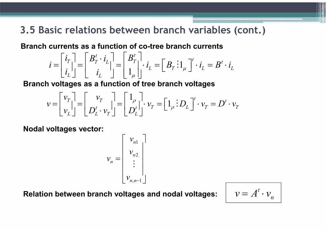
3.5 Basic relations between branch variables (cont.)
11
tttT T tT L
L T L L
L L
i BB ii i B i B i
i i
M
11
tT T t
T L T Tt t
L L T L
v vv v D v D v
v D v D
M
Branch currents as a function of co-tree branch currents
Branch voltages as a function of tree branch voltages
Nodal voltages vector:
1
2
, 1
n
n
n
n n
v
vv
v
M
Relation between branch voltages and nodal voltages:t
nv A v
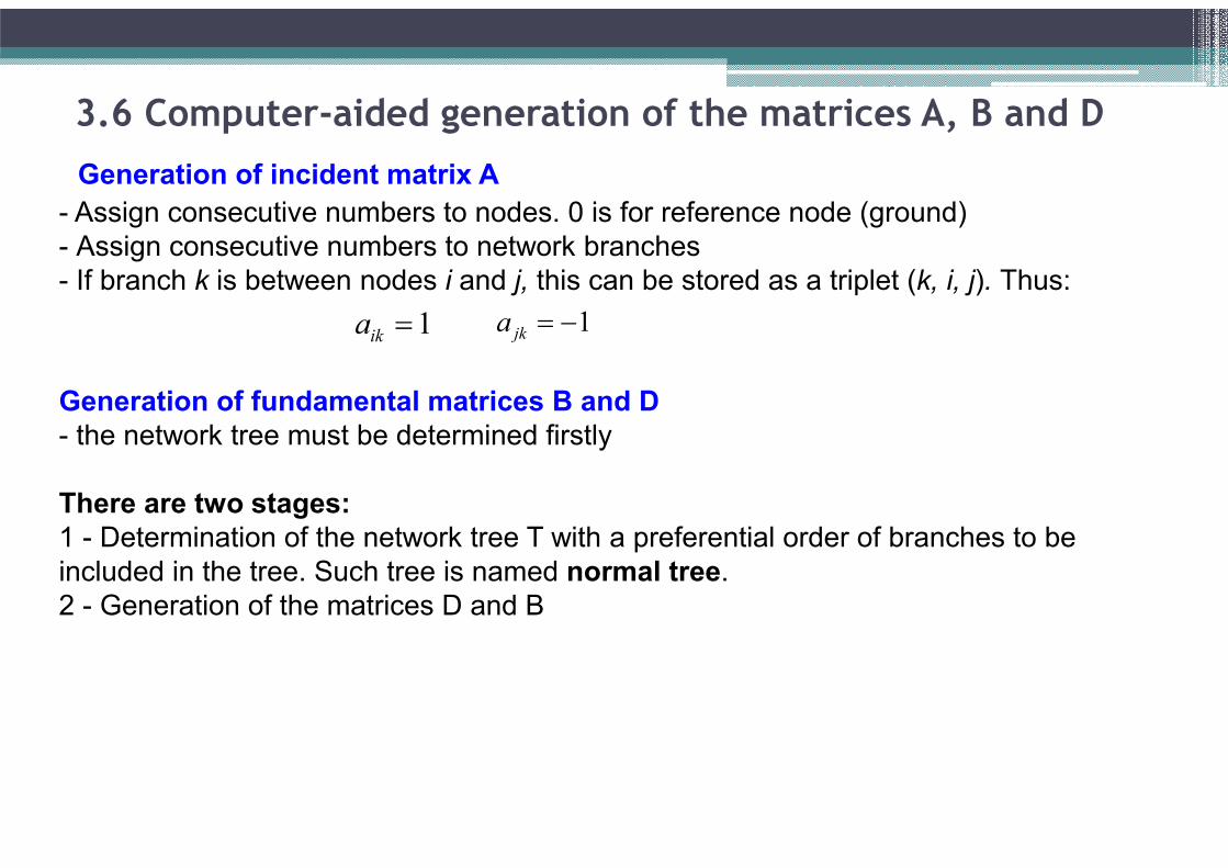
3.6 Computer-aided generation of the matrices A, B and D
Generation of incident matrix A
- Assign consecutive numbers to nodes. 0 is for reference node (ground)
- Assign consecutive numbers to network branches
- If branch k is between nodes i and j, this can be stored as a triplet (k, i, j). Thus:
1ika 1jka
Generation of fundamental matrices B and D
- the network tree must be determined firstly
There are two stages:
1 - Determination of the network tree T with a preferential order of branches to be
included in the tree. Such tree is named normal tree.
2 - Generation of the matrices D and B

3.6.1 Network tree determination
•The network tree can be determined starting from A matrix
•The columns of A matrix are rearranged in the preferential order of branches to be
included in the tree:
Independent voltage sources
Controlled voltage sources
Capacitors
Resistors
Inductors
Controlled current sources
Independent current sources
9 1 6 2 5 8 10 3 4 7
1
2
1
V C C R R R L I J J
A
n
M
Example:
• In the matrix A first independent n-1
columns are determined. This is possible
by transforming A matrix into an echelon
form matrix using elementary row
operations:
• row interchanging
• multiply a row with a non-zero value
• multiply a row with a non-zero value
and add to another row
1 2 3
1 1 x x x x x x x
2 0 0 1 x x x x x
3 0 0 0 1 x x x x
0 0 0 0 0 0 1 x
0 0 0 0 0 0 0 0
kc c c c
Q
k
L L
L L
L L
M M M M M M M M
L L
L L
Echelon form matrix:

Network tree determination – cont.
Algorithm to transform the matrix A into echelon form matrix
Let As a submatrix of A. Initial As=A
• Step 1: the first nonzero column is searched in As. Name c this column.
• Step 2: In column c, first non-zero value is searched from up to down, for
example in the row r. If r=1 go to step 4.
• Step 3: Within As, rows 1 and r are interchanged.
• Step 4: If element (1,c) is -1 the row 1 from As is multiplied by -1.
• Step 5: In column c all non-zero elements below first row from As are reduced to
zero.
• Step 6: New As matrix is defined. It consist of rows below first row from old As
and columns situated at the right side of column c. If new As doesn’t exist,
algorithm is finished, else go to step 1.
•Independent columns in A are the
columns of first element of 1 from each
row within echelon form matrix
• Branches corresponding to these
columns form the network tree.

Network tree determination – Example
3 2 4 8 1 9 10 5 6 7
2 1
1 5 5
1 0 1 1 0 1 0 0 1 0 0
2 1 1 0 0 1 0 0 0 0 0
3 0 0 0 0 0 0 0 0 1 1
4 0 0 0 1 0 1 0 1 1 0
5 1 0 1 0 0 1 1 0 0 0
L L
L L L
V C C C R R R L L I
A
Matrix A with columns arranged in the preferential order of branches:

Network tree determination – Example (cont.)
Transform matrix A into echelon form using elementary row operations:
Normal tree: V3, C2, C8, R9, L6
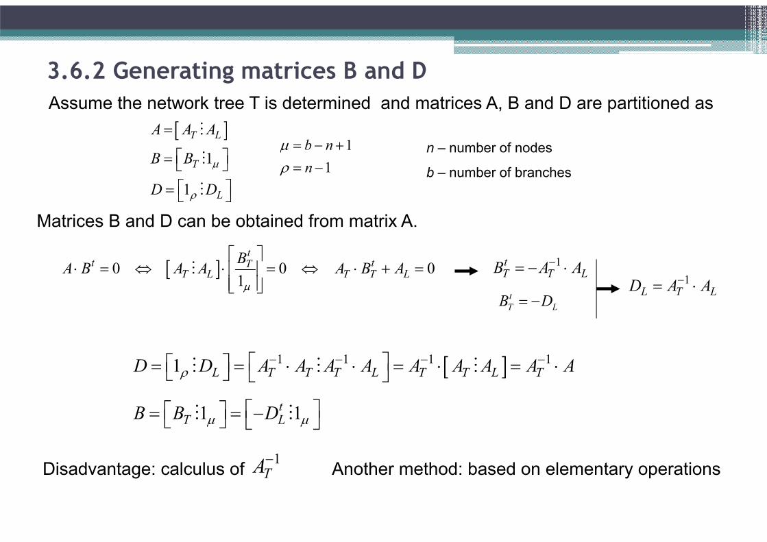
3.6.2 Generating matrices B and D
Assume the network tree T is determined and matrices A, B and D are partitioned as
1
1
T L
T
L
A A A
B B
D D
M
M
M
1
1
b n
n
n – number of nodes
b – number of branches
Matrices B and D can be obtained from matrix A.
0 0 01
tt tT
T L T T L
BA B A A A B A
M
1tT T LB A A
t
T LB D
1L T LD A A
1 1 1 11 L T T T L T T L TD D A A A A A A A A A M M M
1 1tT LB B D M M
Disadvantage: calculus of1TA
Another method: based on elementary operations
3.6.2 Generating matrices B and D (cont.)
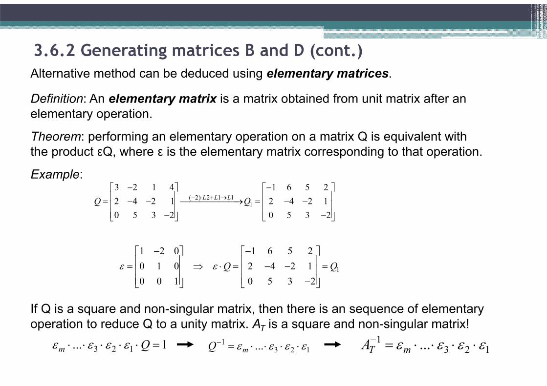
Alternative method can be deduced using elementary matrices.
Definition: An elementary matrix is a matrix obtained from unit matrix after an
elementary operation.
Theorem: performing an elementary operation on a matrix Q is equivalent with
the product εQ, where ε is the elementary matrix corresponding to that operation.
Example:
( 2) 2 1 11
3 2 1 4 1 6 5 2
2 4 2 1 2 4 2 1
0 5 3 2 0 5 3 2
L L LQ Q
1
1 2 0 1 6 5 2
0 1 0 2 4 2 1
0 0 1 0 5 3 2
Q Q
If Q is a square and non-singular matrix, then there is an sequence of elementary
operation to reduce Q to a unity matrix. AT is a square and non-singular matrix!
3 2 1... 1m Q 13 2 1...mQ
13 2 1...T mA
3.6.2 Generating matrices B and D (cont.)
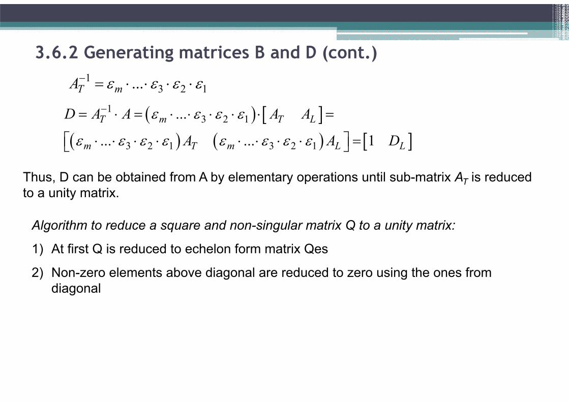
13 2 1...T mA
13 2 1
3 2 1 3 2 1
...
... ... 1
T m T L
m T m L L
D A A A A
A A D
Thus, D can be obtained from A by elementary operations until sub-matrix AT is reduced
to a unity matrix.
Algorithm to reduce a square and non-singular matrix Q to a unity matrix:
1) At first Q is reduced to echelon form matrix Qes
2) Non-zero elements above diagonal are reduced to zero using the ones from
diagonal
3.6.2 Generating matrices B and D (cont.)
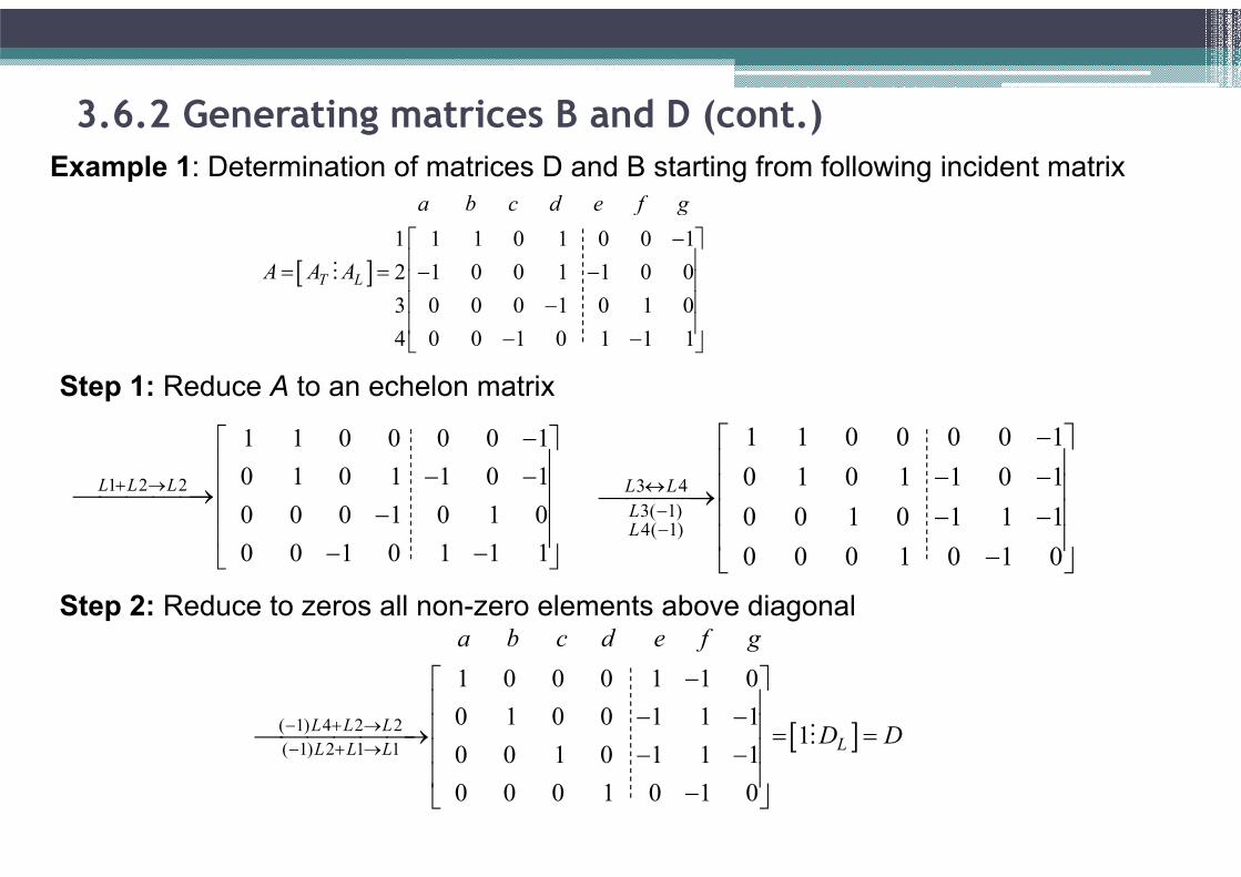
Example 1: Determination of matrices D and B starting from following incident matrix
1 1 1 0 1 0 0 1
2 1 0 0 1 1 0 0
3 0 0 0 1 0 1 0
4 0 0 1 0 1 1 1
T L
a b c d e f g
A A A
M
Step 1: Reduce A to an echelon matrix
1 2 2
1 1 0 0 0 0 1
0 1 0 1 1 0 1
0 0 0 1 0 1 0
0 0 1 0 1 1 1
L L L
3 4
3( 1)4( 1)
1 1 0 0 0 0 1
0 1 0 1 1 0 1
0 0 1 0 1 1 1
0 0 0 1 0 1 0
L L
LL
Step 2: Reduce to zeros all non-zero elements above diagonal
( 1) 4 2 2
( 1) 2 1 1
1 0 0 0 1 1 0
0 1 0 0 1 1 11
0 0 1 0 1 1 1
0 0 0 1 0 1 0
L L LLL L L
a b c d e f g
D D
M

3.6.2 Generating matrices B and D (cont.)
1 1 1 0 1 0 0
1 1 1 1 1 1 0 1 0
0 1 1 0 0 0 1
tT L
a b c d e f g
B B D
M M
Loops matrix B
Example 2
3 2 4 8 1 9 10 5 6 7
1 0 1 1 0 1 0 0 1 0 0
2 1 1 0 0 1 0 0 0 0 0
3 0 0 0 0 0 0 0 0 1 1
4 0 0 0 1 0 1 0 1 1 0
5 1 0 1 0 0 1 1 0 0 0
V C C C R R R L L I
A
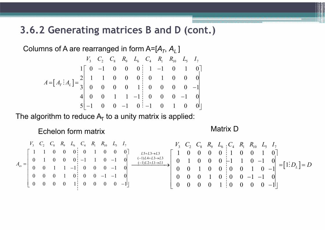
3.6.2 Generating matrices B and D (cont.)
Columns of A are rearranged in form A=[AT, AL ]
3 2 8 9 6 4 1 10 5 7
1 0 1 0 0 0 1 1 0 1 0
2 1 1 0 0 0 0 1 0 0 0
3 0 0 0 0 1 0 0 0 0 1
4 0 0 1 1 1 0 0 0 1 0
5 1 0 0 1 0 1 0 1 0 0
T L
V C C R L C R R L I
A A A
M
The algorithm to reduce AT to a unity matrix is applied:
3 2 8 9 6 4 1 10 5 7
1 1 0 0 0 0 1 0 0 0
0 1 0 0 0 1 1 0 1 0
0 0 1 1 1 0 0 0 1 0
0 0 0 1 0 0 0 1 1 0
0 0 0 0 1 0 0 0 0 1
es
V C C R L C R R L I
A
Echelon form matrix
3 2 8 9 6 4 1 10 5 7
5 3 3
( 1) 4 3 3
( 1) 2 1 1
1 0 0 0 0 1 0 0 1 0
0 1 0 0 0 1 1 0 1 01
0 0 1 0 0 0 0 1 0 1
0 0 0 1 0 0 0 1 1 0
0 0 0 0 1 0 0 0 0 1
L L L
L L L
L L L
L
V C C R L C R R L I
D D
M
Matrix D

3 2 8 9 6 4 1 10 5 7
1 1 0 0 0 1 0 0 0 0
0 1 0 0 0 0 1 0 0 01 1
0 0 1 1 0 0 0 1 0 0
1 1 0 1 0 0 0 0 1 0
0 0 1 0 1 0 0 0 0 1
t
T L
V C C R L C R R L I
B B D
M M
3.6.2 Generating matrices B and D (cont.)
Loops matrix: can be written directly from D, taking into accountt
T LB D