computed tomography cse 5780 medical imaging systems and signals ehsan ali and guy hoenig 1
TRANSCRIPT

1
Computed Tomography
CSE 5780 Medical Imaging Systems and Signals
Ehsan Ali and Guy Hoenig
2
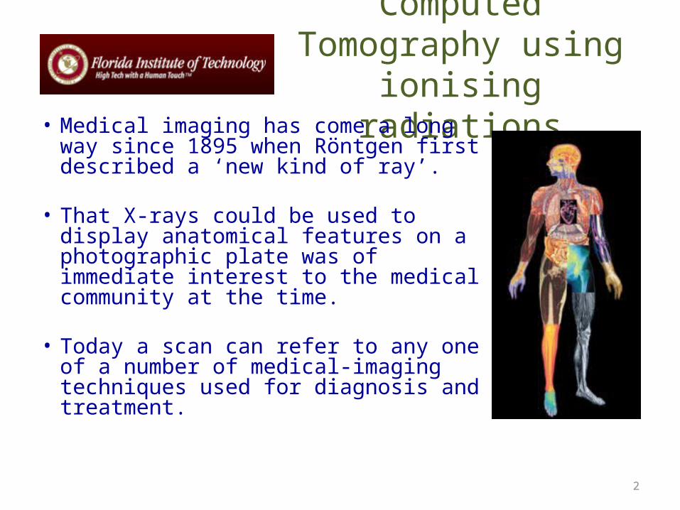
Computed Tomography using ionising radiations
• Medical imaging has come a long way since 1895 when Röntgen first described a ‘new kind of ray’.
• That X-rays could be used to display anatomical features on a photographic plate was of immediate interest to the medical community at the time.
• Today a scan can refer to any one of a number of medical-imaging techniques used for diagnosis and treatment.

3
Instrumentation(Digital Systems)
• The transmission and detection of X-rays still lies at the heart of radiography, angiography, fluoroscopy and conventional mammography examinations.
• However, traditional film-based scanners are gradually being replaced by digital systems
• The end result is the data can be viewed, moved and stored without a single piece of film ever being exposed.

4
CT Imaging
• Goal of x-ray CT is to reconstruct an image whose signal intensity at every point in region imaged is proportional to μ (x, y, z), where μ is linear attenuation coefficient for x-rays.
• In practice, μ is a function of x-ray energy as well as position and this introduces a number of complications that we will not investigate here.
• X-ray CT is now a mature (though still rapidly developing) technology and a vital component of hospital diagnosis.

5
Comparisons of CT Generations
Comparison of CT GenerationsGeneration Source Source
CollimationDetector Detector
CollimationSource-Detector Movement
Advantages Disadvantages
1G Single x-ray tube Pencil beam Single None Move linearly and rotate in unison
Scattered energy is undetected
Slow
2G Single x-ray tube Fan beam, not enough to cover FOV
Multiple Collimated to source direction
Move linearly and rotate in unison
Faster than 1G Lower efficiency and larger noise because of the collimators in directors
3G Single x-ray tube Fan beam, enough to cover FOV
Many Collimated to source direction
Rotate in synchrony Faster than 2G, continuous rotation using slip ring
Moe expensive than 2G, low efficiency
4G Single x-ray tube Fan beam covers FOV
Stationary ring of detectors
Cannot collimate detectors
Detectors are fixed, source rotates
Higher efficiency than 3G
High scattering since detectors are not collimated
5G (EBCT) Many Tungsten anodes in a single large tube
Fan beam Stationary ring of detectors
Cannot collimate detectors
No moving parts Extremely fast, capable of stop-action imaging of beating heart
High cost, difficult to calibrate
6G (Spiral CT) 3G/4G 3G/4G 3G/4G 3G/4G 3G/4G plus linear patient table motion
Fast 3D images A bit more expensive
7G (Multi-slice CT)
Single x-ray tube Cone beam Multiple arrays of detectors
Collimated to source direction
3G/4G/6G motion Fast 3D images Expensive

6
Four generations of CT scanner

7
X-rays CT - 1st Generation•Single X-ray Pencil Beam•Single (1-D) Detector set at 180 degrees opposed
•Simplest & cheapest scanner type but very slow due to •Translate(160 steps) •Rotate (1 degree)•~ 5minutes (EMI CT1000)
•Higher dose than fan-beam scanners
•Scanners required head to be surrounded by water bag
8
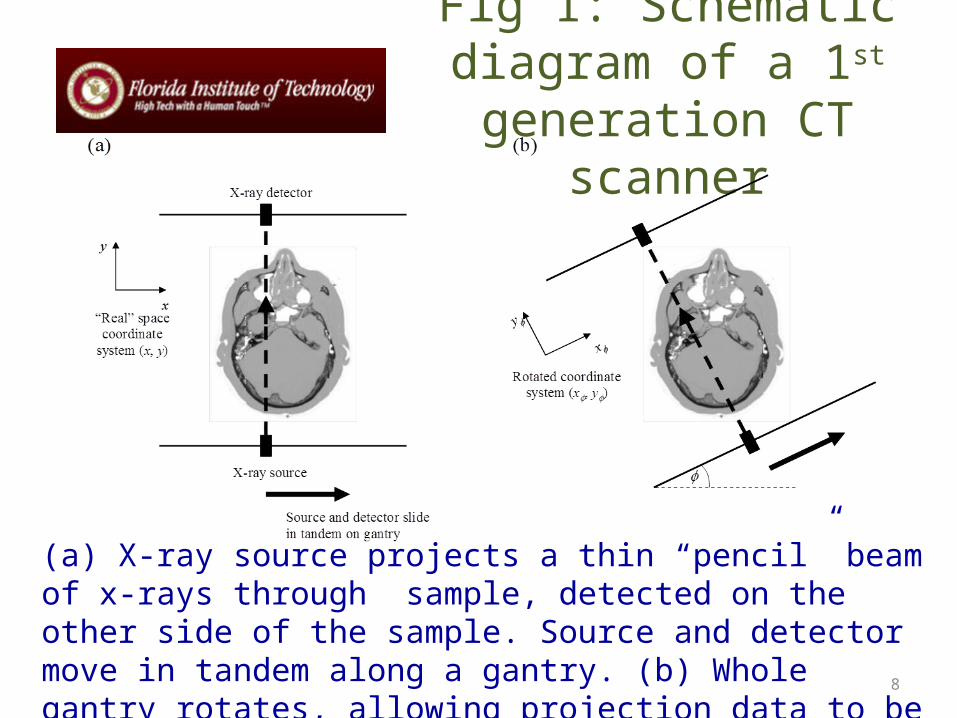
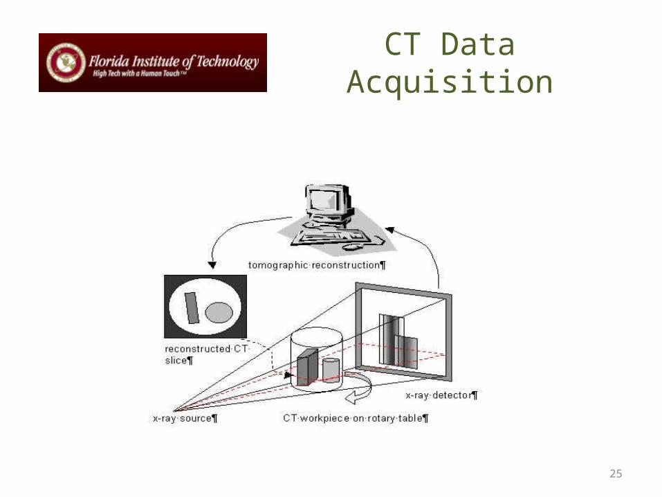
Fig 1: Schematic diagram of a 1st generation CT scanner
(a) X-ray source projects a thin “pencil” beam of x-rays through sample, detected on the other side of the sample. Source and detector move in tandem along a gantry. (b) Whole gantry rotates, allowing projection data to be acquired at different angles.

9
First Generation CT Scanner

10
First-generation CT Apparatus
dyyxIxI ),(exp)( 0

11
Further generations of CT scanner
• The first-generation scanner described earlier is capable of producing high-quality images. However, since the x-ray beam must be translated across the sample for each projection, the method is intrinsically slow.
• Many refinements have been made over the years, the main function of which is to dramatically increase the speed of data acquisition.

12
Further generations of CT scanner (cont’d)
• Scanner using different types of radiation (e.g., fan beam) and different detection (e.g., many parallel strips of detectors) are known as different generations of X-ray CT scanner. We will not go into details here but provide only an overview of the key developments.
13
Second Generation CT scanner

14
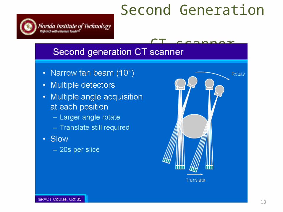
X-rays CT - 2nd Generation (~1980)
•Narrow Fan Beam X-Ray
•Small area (2-D) detector
•Fan beam does not cover full body, so limited translation still required
•Fan beam increases rotation step to ~10 degrees
•Faster (~20 secs/slice) and lower dose
•Stability ensured by each detector seeing non-attenuated x-ray beam during scan

15
Third Generation CT Scanner

16
X-rays CT - 3rd Generation (~1985)

17
X-rays CT - 3rd Generation (~1985)

18
X-rays CT - 3rd Generation
•Wide-Angle Fan-Beam X-Ray
•Large area (2-D) detector
•Rotation Only - beam covers entire scan area
•Even faster (~5 sec/slice) and even lower dose
•Need very stable detectors, as some detectors are always attenuated•Xenon gas detectors offer best stability (and are inherently focussed, reducing scatter)•Solid State Detectors are more sensitive - can lead to dose savings of up to 40% - but at the risk of ring artefacts

19
X-rays CT - 3rd Generation Spiral

20
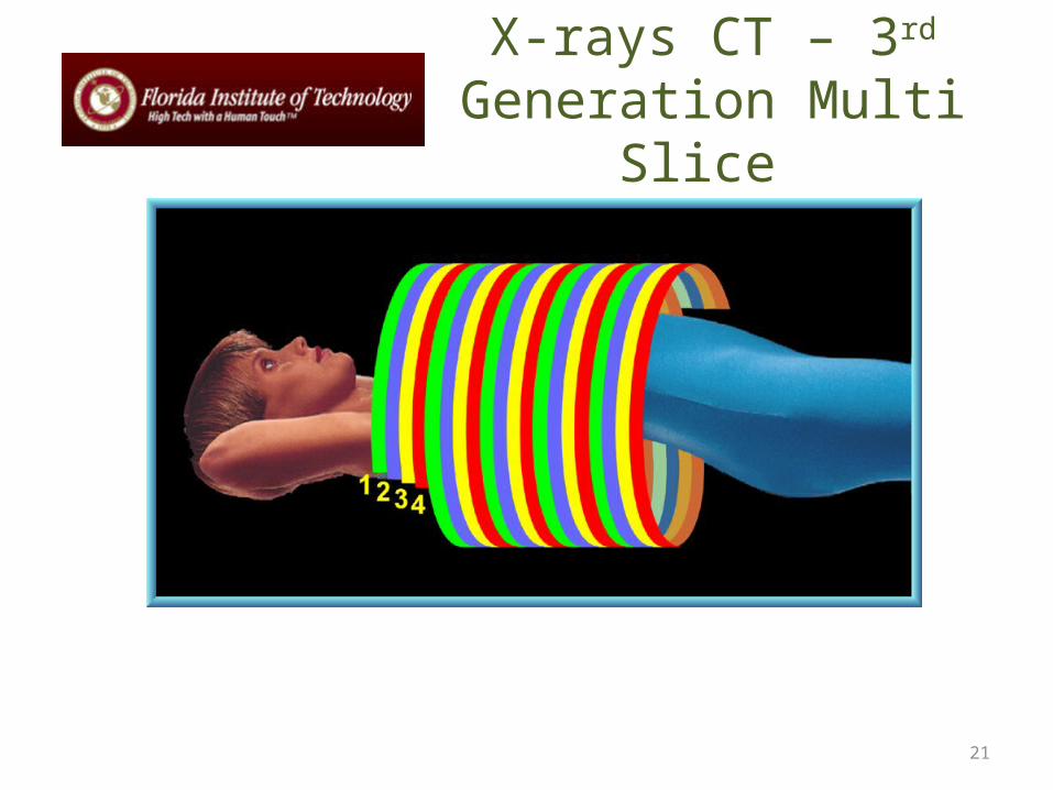
X-rays CT – 3rd Generation Multi Slice
Latest Developments - Spiral, multislice CT Cardiac CT
21
X-rays CT – 3rd Generation Multi Slice

22
Fourth Generation CT Scanners

23
X-rays CT - 4th Generation (~1990)
•Wide-Angle Fan-Beam X-Ray: Rotation Only
•Complete 360 degree detector ring (Solid State - non-focussed, so scatter is removed post-acquisition mathematically)
•Even faster (~1 sec/slice) and even lower dose
•Not widely used – difficult to stabilise rotation + expensive detector
•Fastest scanner employs electron beam, fired at ring of anode targets around patient to generate x-rays.
•Slice acquired in ~10ms - excellent for cardiac work
X-rays CT - Electron Beam 4th Generation

24
X-Ray Source and Collimation
25
CT Data Acquisition

26
CT Detectors: Detector Type

27
Xenon Detectors

28
Ceramic Scintillators

29
CT Scanner Construction: Gantry, Slip Ring, and Patient Table

30
Reconstruction of CT Images: Image Formation
REFERENCE DETECTOR
REFERENCE DETECTOR
ADCPREPROCESSOR
COMPUTER
RAW DATA
CONVOLVED DATABACK PROJECTORRECONSTRUCTED DATA
PROCESSORS
DISK TAPE DAC CRT DISPLAY
31
The Radon transformation
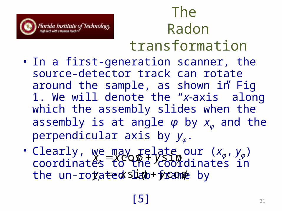
• In a first-generation scanner, the source-detector track can rotate around the sample, as shown in Fig 1. We will denote the “x-axis” along which the assembly slides when the assembly is at angle φ by xφ and the perpendicular axis by yφ.
• Clearly, we may relate our (xφ, yφ) coordinates to the coordinates in the un-rotated lab frame by
[5]
cossin
sincos
yxy
yxx
r
r

32
Figure 2: Relationship between Real Space and
Radon Space
x
yy
x
Typical path of X-rays through sample, leading to detected intensity I(x)
x
Convert I(x) to (x)
Store the result (x) at the point (x ) in Radon space
Real (Image) Space Radon Space
Highlighted point on right shows where the value λφ (xφ) created by passing the x-ray beam through the sample at angle φ and point xφ is placed. Note that, as is conventional, the range of φ is [-π / 2, +π / 2], since the remaining values of φ simply duplicate this range in the ideal case.

33
• Hence, the “projection signal” when the gantry is at angle φ is
[6]
• We define the Radon transform as
[7]
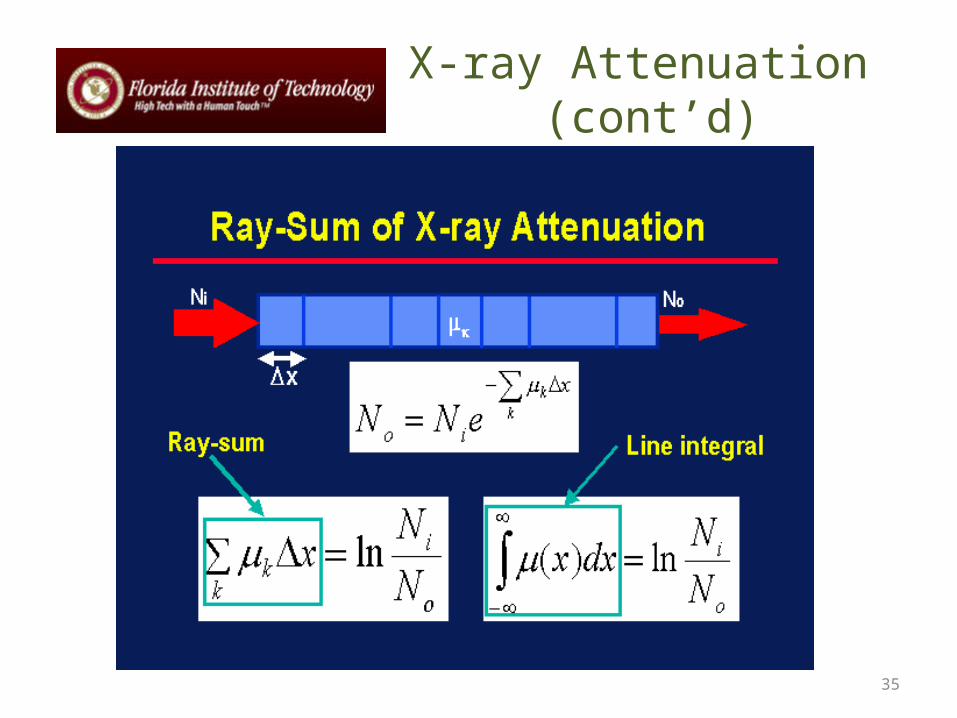
dyyxIxI ),(exp)( 0
0sample
)(ln),()(
I
xIdyyxx

34
Attenuation (x-ray intensity)
35
X-ray Attenuation (cont’d)

36
Radon Space
• We define a new “space”, called Radon space, in much the same way as one defines reciprocal domains in a 2-D Fourier transform. Radon space has two dimensions xφ and φ . At the general point (xφ, φ), we “store” the result of the projection λφ(xφ).
• Taking lots of projections at a complete range of xφ and φ “fills” Radon space with data, in much the same way that we filled Fourier space with our 2-D MRI data.

37
CT ‘X’ Axis
‘X’Axis
38
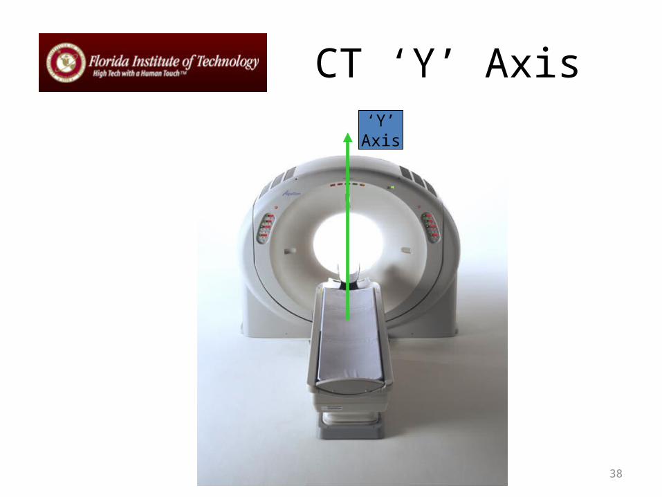
CT ‘Y’ Axis‘Y’
Axis

39
CT ‘Z’ Axis
‘Z’Axis
40
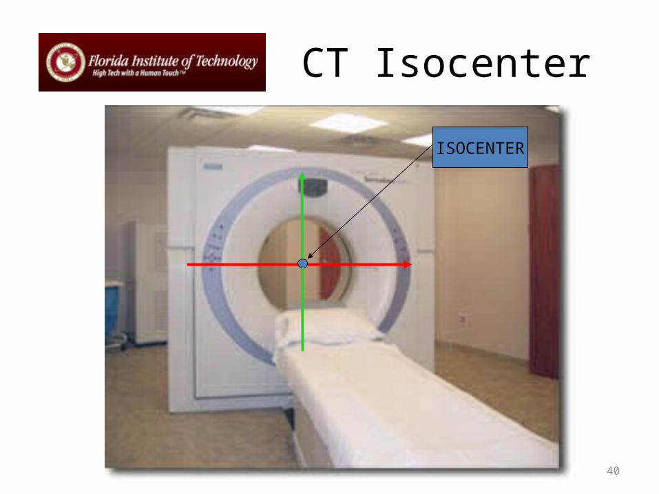
CT Isocenter
ISOCENTER

41
Fig 3. Sinograms for sample consisting of a small number
of isolated objects.
y
x x
Real (Image) Space Radon Space
Single point (x0, y0)
Corresponding sinogram track
In this diagram, the full range of φ is [-π, +π ] is displayed.

42
Relationship between “real space” and Radon space
• Consider how the sinogram for a sample consisting of a single point in real (image) space will manifest in Radon space.
• For a given angle φ, all locations xφ lead to λφ(xφ) = 0, except the one coinciding with the projection that goes through point (x0, y0) in real space. From Equation 5, this will be the projection where xφ = x0 cos φ + y0 sin φ.

43
• Thus, all points in the Radon space corresponding to the single-point object are zero, except along the track
[8]
where R = (x2 + y2)1/2 and φ0 = tan-1 ( y / x).
• If we have a composite object, then the filled Radon space is simply the sum of all the individual points making up the object (i.e. multiple sinusoids, with different values of R and φ0). See Fig 3 for an illustration of this.
)cos(sincos 000 Ryxx

44
Reconstruction of CT images (cont’d)
• This is performed by a process known as back-projection, for which the procedure is as follows:
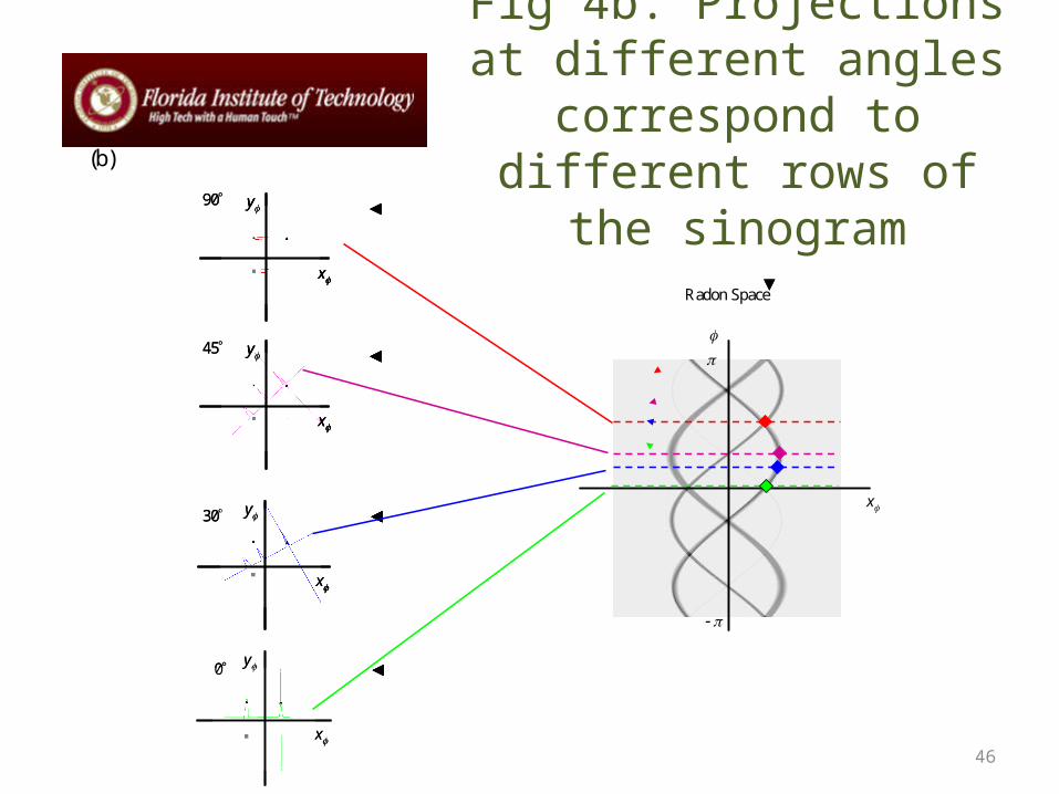
• Consider one row of the sinogram, corresponding to angle φ. Note how in Fig 3, the value of the Radon transform λφ(xφ) is represented by the grey level of the pixel. When we look at a single row (i.e., a 1-D set of data), we can draw this as a graph — see Fig 4(a). Fig 4(b) shows a typical set of such line profiles at different projection angles.

45
Fig 4a. Relationship of 1-D projection through the
sample and row in sinogram
y
x x
Real (Image) Space Radon Space
0Beam path corresponds to peak in projection, with result stored in Radon space
Entire x-profile (i.e., set of projections for all values of xf ) is stored as a row in Radon space
(a)
46
Fig 4b. Projections at different angles correspond to different
rows of the sinogram
x
Radon Space
y
x
0 y
x
0
y
x
30 y
x
y
x
y
x
30
y
x
45 y
x
y
x
y
x
45
y
x
90 y
x
y
x
y
x
90
(b)

47
Fig 4c. Back-projection of sinogram rows to form an image. The high-intensity areas of image correspond to crossing points of all three back-projections of
profiles.

48
General Principles of Image Reconstruction
• Image Display - Pixels and voxels

49
PIXEL Size Dependencies:
• MATRIX SIZE• FOV

50
PIXEL vs VOXEL
PIXELVOXEL

51
VOXEL Size Dependencies
• FOV• MATRIX SIZE• SLICE THICKNESS


53
Reconstruction Concept
Ц CT#RECONSTRUCTION

54
CT and corresponding pixels in image

55
Simple numerical example

56
µ To CT number

57
CT Number Flexibility
• We can change the appearance of the image by varying the window width (WW) and window level (WL)
• This spreads a small range of CT numbers over a large range of grayscale values
• This makes it easy to detect very small changes in CT number

58
Windowing in CT

59
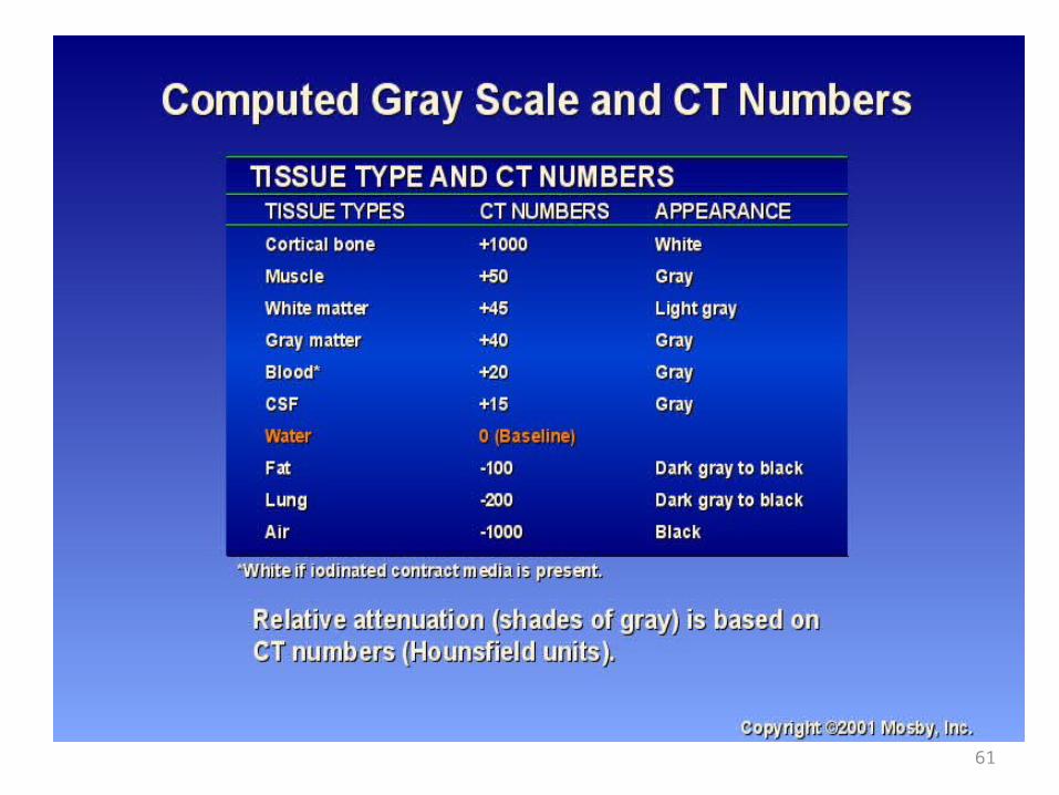
CT Numbers
Linear attenuation coefficient of each tissue pixel is compared with that of water:
w
wtNoCT
1000.

60
CT Number Window
61

62
Example values of μt:
At 80 keV: μbone = 0.38 cm-1
μwater = 0.19 cm-1
The multiplier 1000 ensures that the CT (or Hounsfield) numbers are whole numbers.

63
Linear Attenuation Coefficient ( cm-1)
• BONE 0.528• BLOOD 0.208• G. MATTER 0.212• W. MATTER 0.213• CSF 0.207• WATER 0.206• FAT 0.185• AIR 0.0004

64
CT # versus Brightness Level
+ 1000
-1000

65
CT in practice

66
SCAN Field Of View (FOV) Resolution
SFOV
67
Display FOV versus Scanning FOV
• DFOV CAN BE EQUAL OR LESS OF SFOV• SFOV – AREA OF MEASUREMENT DURING
SCAN • DFOV - DISPLAYED IMAGE

68
Image Quality in CT
69
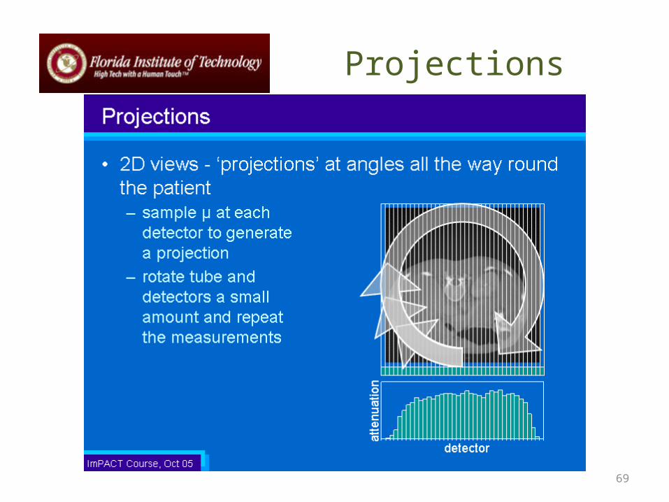
Projections

70
Back Projection
• Reverse the process of measurement of projection data to reconstruct an image
• Each projection is ‘smeared’ back across the reconstructed image

71
Back Projection

72
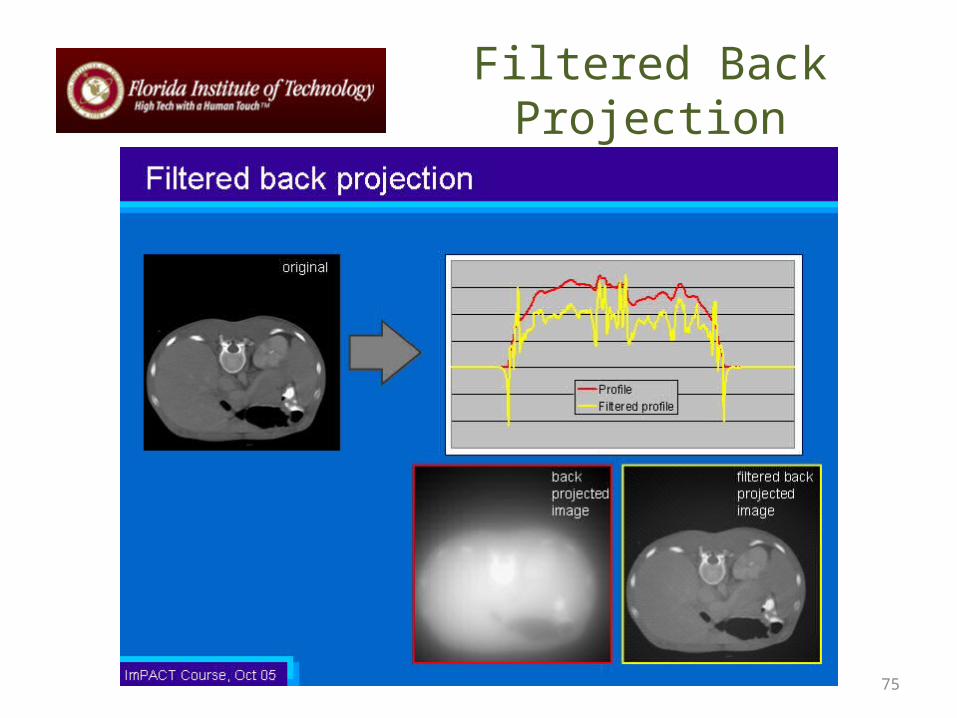
Filtered Back Projection
• Back projection produces blurred trans-axial images
• Projection data needs to be filtered before reconstruction
• Different filters can be applied for different diagnostic purposes• Smoother filters for viewing soft tissue • Sharp filters for high resolution imaging
• Back projection process same as before

73
Filtered Back Projection

74
Filtered Back Projection
75
Filtered Back Projection

76
Summary and Key Points
• A tomogram is an image of a cross-sectional plane or slice within or through the body • X-Ray computed tomography (CT) produces tomograms of the distribution of linear
attenuation coefficients, expressed in Hounsfield units.• There are currently 7 generations of CT scanner design, which depend on the relation
between the x-ray source and detectors, and the extent and motion of the detectors (and patient bed).
• The basic imaging equation is identical to that for projection radiography; the difference is that the ensemble or projections is used to reconstruct cross-sectional images.
• The most common reconstruction algorithm is filtered back projection, which arises from the projection slice theorem.
• In practice, the reconstruction algorithm must consider the geometry of the scanner–parallel-beam, fan-beam,helical-scan, or cone-beam.
• As in projection radiography, noise limits an image’s signal to noise ratio.• Other artifacts include aliasing , beam hardening, and – as in projection radiography –
inclusion of the Compton scattered photons.

77
Cone Beam CT: Introduction
78
CT Basic Principle
Point 1: Purpose of CT and Basic principle
Point 2: The internal structure of an object can be reconstructed from multiple projections of the object
Point 3: Computerized Tomography, or CT is the preferred current technology

79
The Basics

80
Current Cone Beam Systems

81
Cone Beam Reconstruction

82
The ‘Z’ Axis

83
Medical CT Vs.Cone Beam CT

84
Medical CT Example

85
Cone Beam CT Example

86
Cone Beam CT example

87
CBCT Advantages over Medical CT

88
References
• University of Surrey: PH3-MI (Medical Imaging): David Bradley Office 18BC04 Extension 3771
• Physical Principles of Computed Tomography• Basic Principles of CT Scanning: ImPACT Course October 2005