computational tool for a mini-windmill study with softpicard/publications/dd18-2008.pdf ·...

Computational Tool for a Mini-Windmill studywith SOFT

M. Garbey, M. Smaoui, N. De Brye, and C. Picard

Department of Computer Science, University of Houston, Houston, TX 77204 [email protected]

1 Introduction and Motivation

In this paper, we present a parallel computational framework for the com-pletely automated design of a Vertical Axis Fluid Turbine (VAFT) . Sim-ulation, Optimum design, Fabrication and Testing (SOFT) of the VAFT isintegrated into a hardware/software environment that can fit into a small of-fice space.The components of the four steps design loop are as follows

1. Simulation: We use a parallel CFD algorithm to run a direct simulationof the fluid structure interaction problem. We derive from that computa-tion the torque and the average rotation speed for a given friction coef-ficient on the rotor shaft and an average flow speed. Our objective is toget the most power out of the windmill, consequently the highest rotationspeed possible.

2. Optimization: We optimize the shape of the blade section with a geneticalgorithm and/or a surface response. The evaluation of the objective func-tion (average rotation speed) corresponds to the direct simulation of theNavier Stokes flow interacting with the rotating turbine, until reaching astationary regime. Because this simulation is compute-intensive, we dis-tribute the evaluation of the objective function for the different shapes(gene or parameter combinations) on a network of computers using anembarrassingly parallel algorithm.

3. Fabrication: The optimization procedure results in a supposedly opti-mum shape in the chosen design space. This shape is sent to a 3-D printerthat fabricates the real turbine. This turbine is set up such that it canbe easily mounted on a standard base equipped with an electric alterna-tor/generator.

4. Testing: The windmill is tested in a mini wind tunnel. The electric outputis measured and a video camera can directly monitor the windmill rotationthrough the transparent wall of the wind tunnel. This information can be

2 M. Garbey, M. Smaoui, N. De Brye, and C. Picard

analyzed by the computer system and comparison with the simulation isassessed. Figure 1 gives a graphical overview of the SOFT concept.

This four-steps loop can be repeated as many times as needed. Eventu-ally, artificial intelligence tools such as Bayesian networks can be added toclose the design loop efficiently. This component would decide when to testother classes of design characterized by the number of blades, the number ofstages in the turbine, the use of baffles to channel the flow etc ... - see Figure 2

Fig. 1. SOFT concept Fig. 2. Collection of VAFT Shapes

We will concentrate here on two dimensional computation with a simplifiedtwo scoop blade that is symmetric with respect to its shaft as in Figure 3.

Fig. 3. Design of the turbine

We have chosen to optimize the VAFT in low speed flow condition, withReynolds number in the range (100 - 2000). We do not need a priori to dealwith complex turbulent flow neither stability issues in the fluid structure in-teraction. One of the possible applications is to power remote sensors with

Computational Tool for a Mini-Windmill study with SOFT 3

VAFT when other energy sources are more difficult to manage. We are alsointerested in low Reynolds number flows that are characteristic of micro airvehicle [Shyy et al.(2007)Shyy, Lian, Tang, Viieru, and Liu].

This project has some obvious pedagogic components that can motivateundergraduate students to do science! However, in reality, a critical step inthe process is obviously the CFD method to test the VAFT performance: thenumerical simulator should be robust, extremely fast but accurate enoughto discriminate bad design from good design. We will discuss an immersedboundary method and domain decomposition solver that we have tentativelydeveloped to satisfy this ambitious program. We first describe the incompress-ible Navier Stokes Solver.

2 Flow Solver

We use the penalty method introduced by Caltagirone and his co-workers[Arquis and Caltagirone(1984)] that is simpler to implement than our pre-vious boundary fitted methods [Garbey and Vassilevski(2001)] and appliesnaturally to flow in a domain with moving walls [Schneider and Farge(2005)].

The flow of incompressible fluid in a rectangular domain Ω = (0, Lx) ×(0, Ly) with prescribed values of the velocity on ∂Ω obeys the NS equations:

∂tU + (U · ∇)U +∇p− ν∇ · (∇U) = f, in Ω

div(U) = 0, in Ω

U = g on ∂Ω,

We denote by U(x, y, t) the velocity with components (u1, u2) and by p(x, y, t)the normalized pressure of the fluid. ν is a kinematic viscosity.

With an immersed boundary approach the domain Ω is decomposed intoa fluid subdomain Ωf and a moving rigid body subdomain corresponding tothe blade Ωb. In the L2 penalty method the right hand side f is a forcingterm that contains a mask function ΛΩb

ΛΩb(x, y) = 1, if (x, y) ∈ Ωb, 0 elsewhere,

and is defined as follows

f = −1ηΛΩb

U − Ub(t). (1)

Ub is the velocity of the moving blade and η is a small positive parameterthat tends to zero.


A formal asymptotic analysis helps us to understand how the penaltymethod matches the no slip boundary condition on the interface Sfb = Ωf

⋂Ωb

as η → 0. Let us define the following expansion:

U = U0 + η U1, p = p0 + η p1.

Formally we obtained at leading order,

1ηΛΩb

U0 − Ub(t) = 0,

that isU0 = Ub, for (x, y) ∈ Ωb.

The leading order terms U0 and p0 in the fluid domain Ωf satisfy the standardset of NS equations:

∂tU0 + (U0 · ∇)U0 +∇p0 − ν∇ · (∇U0) = 0, in Ωf

div(U0) = 0, in Ω.At next order we have in Ωb,

∇p0 + U1 +Qb = 0, (2)

whereQb = ∂tUb + (Ub · ∇)Ub − ν∇ · (∇Ub).

Further the wall motion Ub must be divergence free which is the case for arigid body. In conclusion, the flow evolution is dominated by the NS equationsin the flow domain, and by the Darcy law with very small permeability insidethe rotor.

In this framework, the efficiency of the NS code relies essentially on the de-sign of robust and efficient parallel solvers for linear operators of the followingtwo types

−ε∆+ δu · ∇+ Id

and

−∆.To be more specific, time stepping uses a multi-step projection scheme. Spacediscretization is done with a staggered grid. The convection is processed withthe method of characteristic. Since the penalty term is linear it is trivial tomake that term implicit in time stepping. Finally we use a combination ofAitken-Schwarz as the domain decomposition solver with block LU decompo-sition per subdomain. We refer to [Hadri and Garbey(2008)] for an extensivereport on the performance of that parallel solver on multiple computer ar-chitecture and a comparison with other solvers such as multigrid or Krylovmethods. We are going now to describe a key aspect that is the Fluid StructureInteraction (FSI) approach we have followed here.


3 FSI

First let us discuss the computation of the torque. The main difficulty with thepenalty method is that the flow field is not differentiable at the fluid structureinterface. The computation of the drag forces exerted on the blade cannot bedone directly with the standard formula

F =∫∂Ωb

σ(U, p) n dγ,

where σ(U, p) = 12ν(∇U + (∇U)t)− p I.

Using the observation of [Angot et al.(1999)Angot, Bruneau, and Fabrie],we can compute this force with an integral on the gradient of pressure insidethe blade:

F = limη→0

∫Ωb

∇ p dx,

which ends up with the simple formula using the momentum equation:

F = limη→0−1η

∫Ωb

U − Ub dx. (3)

The computation of the torque is done by summing up the contributionof (3) to the torque, cell-wise and inside the blade. We take into account onlythe interior cells to avoid the singularity at the wall and leave out from thecalculation all the cells that intersect the boundary of the blade ∂Ωb. Theverification on the computational efficiency of this technic has been done withstatic torque calculation. We checked that when the penalty parameter goesto zero, η → 0, the numerical error is rapidly dominated by the grid accuracy.As h → 0, we observe first order convergence. Finally we did compare ourtorque computation with Adina’s computation. Adina is a commercial finiteelement code that uses an arbitrary Lagrangian-Eulerian formulation withdisplacements compatibility and traction equilibrium at the blade interface.

We did some fine mesh calculation with Adina of the static toque, i.e forfixed orientation of the blade, and use that numerical solution as reference. Wefound that it was easy to maintain a 10% accuracy compare to the referencesolution computed with Adina with moderated grid size and Reynolds numberof order a few hundreds, provided that the tip of the blade had a thickness ofat least 3 to 4 mesh points.

Let us discuss now the FSI algorithm based on this torque calculation. Itis classic to apply the second Newton law and advance the rotor accordingly:we alternate then the flow solver and solid rotation. Unfortunately, while thepenalty method is very robust, this solution is ill-conditioned, due to thestiffness of the coupling and sensitivity to the noisy calculation of the Torque.As a matter of fact, we can expect small high frequency oscillation in time of


the torque calculation with rotating blades as Cartesian cell enter/leaves thedomain of computation Ωb.

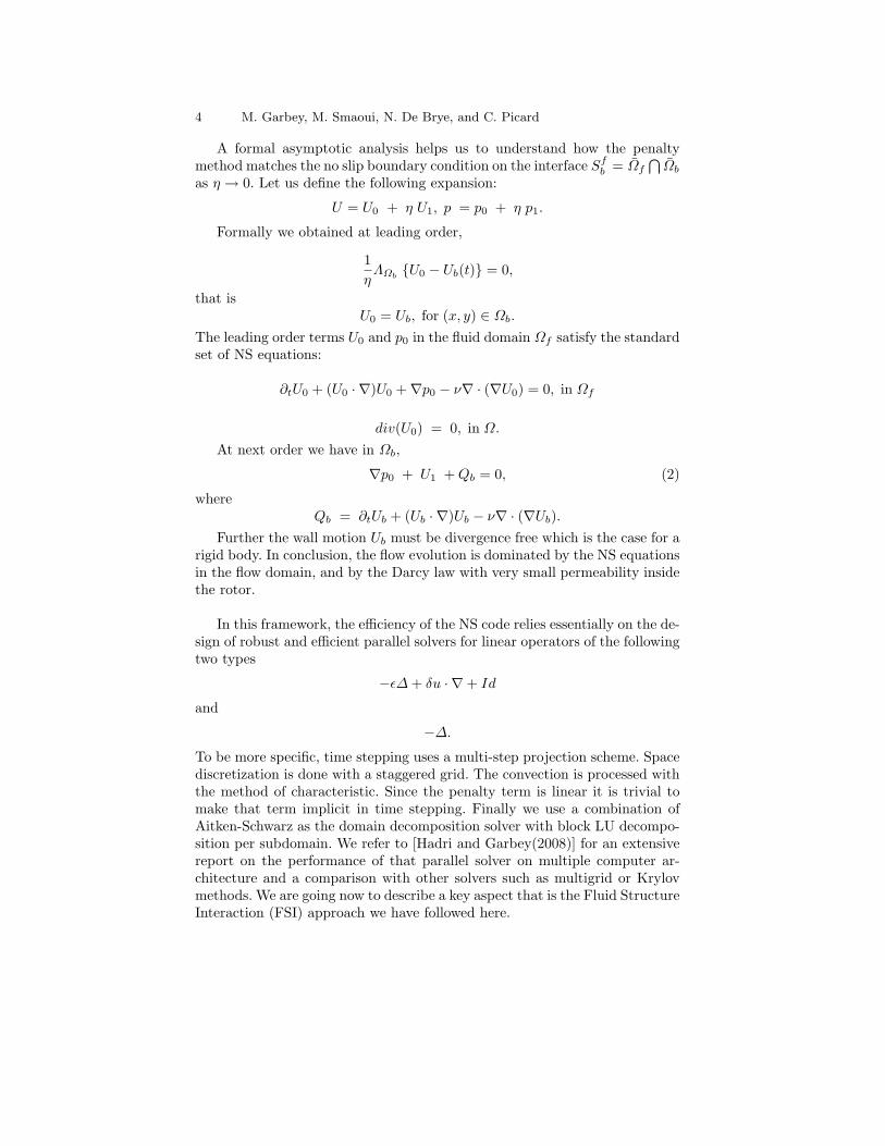
”Thinking parallel” leads to a completely different new solution to solvethis FSI. Based on extensive FSI simulations with Adina of various bladedesigns, we have observed that the velocity of the rotor can be representedaccurately with few Fourier modes:

∂Φ

∂t= Φ0 + Φ1 sin(Θ) + Φ2 cos(Θ) + ....

Figure 4 gives a representative example of such an Adina calculation ofthe rotating velocity speed of the blade. Since we are interested in comparingdesign to take decision, it does not take a lot of accuracy to compare bladeperformances[Queipo et al.(2005)Queipo, Haftka, Shyy, Goel, Vaidyanathan, and Kevin].

Fig. 4. Comparison of various Blades at different Reynolds number

Our solution is then to apply a forcing speed to the blade and computethe torque exerted on the rotor. We first generate a surface response thatapproximates the torque with a family of a few coefficient in the Fourierexpansion. The idea is second to optimize the periodic rotating speed ∂Φ

∂tfunction on the surface response that satisfies at best the second Newton law:

Min(φ0,φ1,φ2,...)||I∂2Φ

∂t2− T ||(0,P ). (4)

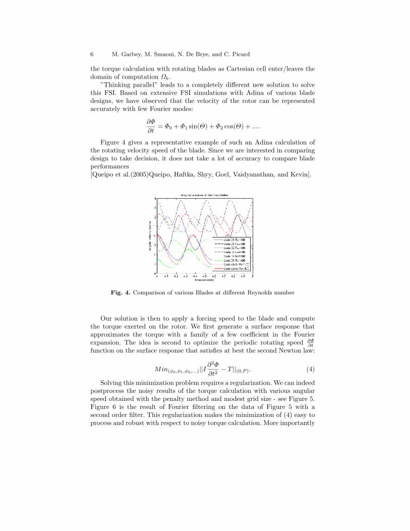
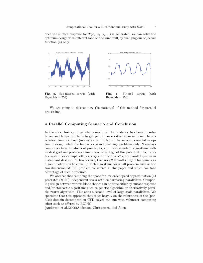
Solving this minimization problem requires a regularization. We can indeedpostprocess the noisy results of the torque calculation with various angularspeed obtained with the penalty method and modest grid size - see Figure 5.Figure 6 is the result of Fourier filtering on the data of Figure 5 with asecond order filter. This regularization makes the minimization of (4) easy toprocess and robust with respect to noisy torque calculation. More importantly


once the surface response for T (φ0, φ1, φ2, ...) is generated, we can solve theoptimum design with different load on the wind mill, by changing our objectivefunction (4) only.

Fig. 5. Non-filtered torque (withReynolds = 250)

Fig. 6. Filtered torque (withReynolds = 250)

We are going to discuss now the potential of this method for parallelprocessing.

4 Parallel Computing Scenario and Conclusion

In the short history of parallel computing, the tendency has been to solvelarger and larger problems to get performance rather than reducing the ex-ectution time for fixed (modest) size problems. The second is needed in op-timum design while the first is for grand challenge problems only. Nowadayscomputers have hundreds of processors, and most standard algorithms withmodest grid size problems cannot take advantage of this potential. The Sicor-tex system for example offers a very cost effective 72 cores parallel system ina standard desktop PC box format, that uses 200 Watts only. This sounds asa good motivation to come up with algorithms for small problem such as thetwo dimension NS FSI problem considered in this paper and which can takeadvantage of such a resource.

We observe that sampling the space for low order speed approximation (4)generates O(100) independent tasks with embarrassing parallelism. Compar-ing design between various blade shapes can be done either by surface responseand/or stochastic algorithms such as genetic algorithm or alternatively parti-cle swarm algorithm. This adds a second level of large scale parallelism. Wespeculate that this approach that relies heavily on the robustness of the (par-allel) domain decomposition CFD solver can run with volunteer computingeffort such as offered by BOINC[Anderson et al.(2006)Anderson, Christensen, and Allen].


To conclude this paper, we have presented the SOFT concept to designVAFT automatically and a domain decomposition algorithm that can be arobust numerical engine for the FSI simulation of the VAFT. We found inour recent experience that this project had a positive impact to motivateour students in science and possibly improve our student enrollment. It issomewhat fascinating to our students to build real turbine with a numericalalgorithm. We are currently running simulations to test the limits of ourFSI/Immersed Boundary approach with Reynolds numbers much larger thanin the present paper. This is, indeed, a very critical issue for the applicability ofour method. However we believe that in principle one can reuse any existingNS codes into our FSI and optimization design framework to tackle largerwindmill designs, that have to run in the turbulent boundary atmosphericlayer where urban VAFTs should operate.

References

[Anderson et al.(2006)Anderson, Christensen, and Allen] David P. Anderson, CarlChristensen, and Bruce Allen. Designing a runtime system for volunteer comput-ing. In SC ’06. Proceedings of the ACM/IEEE SuperComputing 2006 Conference,pages 33–43, November 2006.

[Angot et al.(1999)Angot, Bruneau, and Fabrie] Philippe Angot, Charles-HenriBruneau, and Pierre Fabrie. A penalization method to take into accountobstacles in incompressible viscous flows. Numerische Mathematik, 81(4):497–520, February 1999.

[Arquis and Caltagirone(1984)] E. Arquis and J.P. Caltagirone. Sur les conditionshydrodynamiques au voisinage d’une interface milieu fluide-milieux poreux: Ap-plication a la convection naturelle. Comptes Rendus de l’Acadmie des SciencesParis, Serie II, 299:1–4, 1984.

[Garbey and Vassilevski(2001)] M. Garbey and Yu.V. Vassilevski. A parallel solverfor unsteady incompressible 3d navier-stokes equations. Parallel Computing, 27(4):363–389, March 2001.

[Hadri and Garbey(2008)] Bilel Hadri and Marc Garbey. A fast navier-stokes flowsimulator tool for image based cfd. to appear in Journal of Algorithms andComputational Technology, 2008.

[Queipo et al.(2005)Queipo, Haftka, Shyy, Goel, Vaidyanathan, and Kevin]Nestor V. Queipo, Raphael T. Haftka, Wei Shyy, Tushar Goel, RajkumarVaidyanathan, and Tucker P. Kevin. Surrogate-based analysis and optimization.Progress in Aerospace Sciences, 41(1):1–28, January 2005.

[Schneider and Farge(2005)] K. Schneider and M. Farge. Numerical simulation ofthe transient flow behaviour in tube bundles using a volume penalization method.Journal of Fluids and Structures, 20(4):555–566, May 2005.

[Shyy et al.(2007)Shyy, Lian, Tang, Viieru, and Liu] Wei Shyy, Yongsheng Lian,Jian Tang, Dragos Viieru, and Hao Liu. Aerodynamics of Low Reynolds NumberFlyers. Cambridge Aerospace Series. Cambridge University Press, Cambridge,MA, 2007.

computational tool for a mini-windmill study with softpicard/publications/dd18-2008.pdf ·...

Documents