computational rheology for pipeline and annular flow 2001
TRANSCRIPT
Computational Rheology for Pipeline and Annular Flow by Wilson C. Chin, Ph.D.
Boston Oxford Auckland Johannesburg Melbourne New Delhi

Gulf Professional Publishing is an imprint of Butterworth-Heinemann
Copyright © 2001 by Butterworth–Heinemann
A member of the Reed Elsevier group
All rights reserved.
No part of this publication may be reproduced, stored in a retrieval system, or trans-mitted in any form or by any means, electronic, mechanical, photocopying, record-ing, or otherwise, without the prior written permission of the publisher.
Recognizing the importance of preserving what has been written,Butterworth–Heinemann prints its books on acid-free paper whenever possible.
Butterworth–Heinemann supports the efforts of American Forests andthe Global ReLeaf program in its campaign for the betterment of trees,forests, and our environment.
Library of Congress Cataloging-in-Publication DataChin, Wilson C.
Computational rheology for pipline and annular flow/ by Wilson C. Chin. p. cm. Includes indexISBN 0-88415-320-7 (alk. Paper)1. Oil well drilling 2. Petroleum pipleines--fluid dynamics--mathematical models3. Wells--fluid dynamics--mathematical models. I. Title.
TN871.C49535 2000622'.3382--dc21 00-06176
British Library Cataloguing-in-Publication DataA catalogue record for this book is available from the British Library.
The publisher offers special discounts on bulk orders of this book.For information, please contact:
Manager of Special SalesButterworth–Heinemann225 Wildwood AvenueWoburn, MA 01801–2041Tel: 781-904-2500Fax: 781-904-2620
For information on all Gulf Professional Publishing publications available, contact our World Wide Web home page at: http://www.gulfpp.com
10 9 8 7 6 5 4 3 2 1
Printed in the United States of America

v
- Dedication -
To:
Mark A. Proett,
Friend and Colleague

vi
vii
Contents
Preface . . . . . . . . . . . . . . . . . . . . . . . . . . . . . . . . . . . . . . . . . . . . . . xi
1. Introduction: Basic Principles and Applications . . . . . . . 1Why Study Rheology?, 5Review of Analytical Results, 7Overview of Annular Flow, 11Review of Prior Annular Models, 13The New Computational Models, 14Practical Applications, 17Philosophy of Numerical Modeling, 20References, 22
2. Eccentric, Nonrotating, Annular Flow . . . . . . . . . . . . . . . 25Theory and Mathematical Formulation, 26Boundary Conforming Grid Generation, 33Numerical Finite Difference Solution, 35Detailed Calculated Results, 37
Example 1. Fully Concentric Annular Flow, 37Example 2. Concentric Pipe and Borehole in the
Presence of a Cuttings Bed, 43Example 3. Highly Eccentric Circular Pipe and
Borehole, 48Example 4. Square Drill Collar in a Circular Hole, 50Example 5. Small Hole, Bingham Plastic Model, 52Example 6. Small Hole, Power Law Fluid, 57Example 7. Large Hole, Bingham Plastic, 59Example 8. Large Hole, Power Law Fluid, 61Example 9. Large Hole with Cuttings Bed, 65
References, 68
viii
3. Concentric, Rotating, Annular Flow . . . . . . . . . . . . . . . . . 69General Governing Equations, 69Exact Solution for Newtonian Flows, 72Narrow Annulus Power Law Solution, 76Analytical Validation, 80Differences Between Newtonian and Power Law Flows, 81More Applications Formulas, 83Detailed Calculated Results, 85
Example 1. East Greenbriar No. 2, 86Example 2. Detailed Spatial Properties Versus “r”, 87Example 3. More of East Greenbriar, 96
References, 99
4. Recirculating Annular Vortex Flows . . . . . . . . . . . . . . . . . 100What Are Recirculating Vortex Flows?, 101Motivating Ideas and Controlling Variables, 102Detailed Calculated Results, 104How to Avoid Stagnant Bubbles, 110A Practical Example, 111References, 112
5. Applications to Drilling and Production . . . . . . . . . . . . . . 113Cuttings Transport in Deviated Wells, 115
Discussion 1. Water-Base Muds , 115Discussion 2. Cuttings Transport Database, 120Discussion 3. Invert Emulsions Versus “All Oil” Muds, 122Discussion 4. Effect of Cuttings Bed Thickness, 125Discussion 5. Why 45o – 60o Inclinations Are Worst, 128Discussion 6. Key Issues in Cuttings Transport, 129
Evaluation of Spotting Fluids for Stuck Pipe, 131Cementing Applications, 135
Example 1. Eccentric Nonrotating Flow, BaselineConcentric Case, 136
Example 2. Eccentric Nonrotating Flow, EccentricCircular Case, 139
Example 3. Eccentric Nonrotating Flow, A SevereWashout, 141
Example 4. Eccentric Nonrotating Flow, Casingwith Centralizers, 142
Example 5. Concentric Rotating Flows,Stationary Baseline, 146
Example 6. Concentric Rotating Flows,Rotating Casing, 150
Coiled Tubing Return Flows, 153
ix
Heavily Clogged Stuck Pipe, 153Conclusions, 155References, 156
6. Bundled Pipelines: Coupled Annular Velocityand Temperature . . . . . . . . . . . . . . . . . . . . . . . . . . . . . . . . . 159Computer Visualization and Speech Synthesis, 160Coupled Velocity and Temperature Fields, 163References, 167
7. Pipe Flow Modeling in General Ducts . . . . . . . . . . . . . . . . 168Newtonian Flow in Circular Pipes, 169Finite Difference Method, 170Newtonian Flow in Rectangular Ducts, 174
Exact Analytical Series Solution, 174Finite Difference Solution, 177Example Calculation, 179
General Boundary Conforming Grid Systems, 180Recapitulation, 183Two Example Calculations, 183
Clogged Annulus and Stuck Pipe Modeling, 186References, 189
8. Solids Deposition Modeling . . . . . . . . . . . . . . . . . . . . . . . . . 190Mudcake Buildup on Porous Rock, 191Deposition Mechanics, 195Sedimentary Transport, 195Slurry Transport, 196Waxes and Paraffins, Basic Ideas, 197Hydrate Control, 201Modeling Concepts and Integration , 203Wax Buildup Due to Temperature Differences, 203Deposition and Flowfield Interaction, 204Detailed Calculated Examples, 205
Simulation 1. Wax Deposition with NewtonianFlow in Circular Duct, 205
Simulation 2. Hydrate Plug with Newtonian Flowin Circular Duct (Velocity Field), 210
Simulation 3. Hydrate Plug with Newtonian Flowin Circular Duct (Viscous Stress Field), 213
Simulation 4. Hydrate Plug with Power Law Flowin Circular Duct, 215
Simulation 5. Hydrate Plug, Herschel-Bulkley Flowin Circular Duct, 218
x
Simulation 6. Eroding a Clogged Bed, 222References, 228
9. Pipe Bends, Secondary Flows, Fluid Heterogeneities . . . . 231Modeling Non-Newtonian Duct Flow in Pipe Bends, 232Straight, Closed Ducts, 232Hagen-Poiseuille Flow Between Planes, 233Flow Between Concentric Plates, 233Flows in Closed Curved Ducts, 236Fluid Heterogeneities and Secondary Flows, 238References, 240
10. Advanced Modeling Methods . . . . . . . . . . . . . . . . . . . . . . . 241Complicated Problem Domains, 241
Singly-Connected Regions, 242Doubly-Connected Regions, 243Triply-Connected Regions, 245
Convergence Acceleration , 246Fast Solutions to Laplace’s Equation, 247Special Rheological Models, 249Software Notes, 252References, 253
Index . . . . . . . . . . . . . . . . . . . . . . . . . . . . . . . . . . . . . . . . . . . . . . . 255
Author Biography . . . . . . . . . . . . . . . . . . . . . . . . . . . . . . . . . . . . 257
xi
Preface
It has been a decade since Borehole Flow Modeling first appeared,integrating modern finite difference methods with advanced techniques incurvilinear grid generation, and applying powerful computational algorithms toannular flow problems encountered in drilling and producing horizontal anddeviated wells. The early work combined essential elements of mathematics andnumerical analysis, also paying careful attention to empirical results obtainedfrom field and laboratory observation, and importantly, always driven by astrong emphasis on “real world” operational problems.
Prior to BFM, workers invoked “slot flow,” “parallel plate,” and “narrowannulus” assumptions to model non-Newtonian flows in eccentric annuli, withlittle success in correlating experimental data. With the new methods, whichsolved the complete flow equations exactly, at least to the extent permitted bynumerical discretization, it was possible to explain the University of Tulsa’sdetailed cuttings transport database in terms of simple physical principles.
Fast forward to the new millennium. Cuttings transport, stuck pipe, andannular flow are even more important because deep subsea drilling imposestighter demands on safety and efficiency. Rheology is more important than eversince drilling fluid characteristics now depend on temperature and pressure. Tomake matters worse, the same subsea applications introduce operationalproblems with severe economical consequences on the “delivery” side. Moreoften than not, thick waxes will deposit unevenly and large hydrate plugs willform in mile-long pipelines. The harsh ocean environment and the lack ofaccessibility make every flow stoppage event a very serious matter involvingmillions of dollars.
While current industry interests focus on the thermodynamics of wax andhydrate crystallization and formation, and to some extent, on the alteredproperties of affected crudes, new rheological models will not be useful untilthey can be used with simulators to study macroscopic flow processes. Forexample, knowing “n” and “k” does not give the flow rate associated with aknown pressure drop when large hydrate plugs or crescent-shaped wax depositsimpede flow within the pipeline. This book uses the methods of BFM to modelnon-Newtonian flow in ducts with arbitrary geometrical cross-sections, e.g.,different classes of blockages associated with different modes of waxdeposition, hydrate formation, and debris accumulation.
xii
As in BFM, our advanced curvilinear grids adapt exactly to the cross-sectional geometry, and allow highly accurate numerical models to beformulated and solved … in seconds. I will focus on practical results. Forexample, we will show that it is not unusual for “25% area blockages” to reducevolumetric flow by 60% to 80% or more. However, our new approachesprovide more than “flow rate versus pressure drop” relationships. We will takeadvantage of new simulation capabilities to design dynamic, time-dependentmodels that show how wax, hydrates, and debris grow or erode withcontinuously changing duct cross-sections, where these changes are imposed bythe velocity and stress environment of general non-Newtonian fluids.
Other applications are possible. For example, natural gas hydrates maybecome an economically viable energy source if potential logistical problemscan be addressed satisfactorily. Some have suggested mixing ground hydrateswith refrigerated crudes to form transportable pipeline slurries. How finelythese solids are ground will affect rheology on the “n and k” level, butsimulation provides actual velocity profiles, power requirements, and pressurelevels for scale-up. Off-design plugging and “start-up conditions” are importantin pipeline operations. The same simulations also produce “snapshots” ofviscous stress fields that tend to erode these structures; thus, for the first time, atool that allows risk evaluation is available. Detailed understanding of the flowenables better characterization of wax and hydrate formation and deposition.
I am indebted to many organizations and individuals that have shaped mytechnical skills, professional interests, and personal perspectives over the years.In particular, I express my gratitude to the Massachusetts Institute ofTechnology, for providing a solid foundation in physics and mathematicalanalysis, and the Boeing Commercial Airplane Company, for the opportunity tolearn modern grid generation and finite difference methods.
I also wish to acknowledge Halliburton Energy Services, particularly SteveAlmond, Ron Morgan, and Harry Smith, and Brown & Root Energy Services,notably Raj Amin, Gee Fung, Tin Win, and Jeff Zhang, for their support indeveloping advanced rheological models, and especially for an environment thatencourages fundamental studies and physical understanding. I am also gratefulto the United States Department of Energy for its support in computervisualization, convergence acceleration, and duct geometry mapping research,provided under Grant No. DE-FG03-99ER82895. The encouragement offeredby Timothy Calk, John Wilson, and James Wright, Gulf Publishing, is alsokindly noted. Finally, I am indebted to my friend and colleague Mark Proett, forlending a critical and sympathetic ear to all my “crazy ideas” over the years.
Wilson C. Chin, Ph.D., M.I.T.
Houston, TexasEmail: [email protected]
1
1
Introduction:Basic Principles and Applications
Students of fluid mechanics learn many laws of nature. For example, theHagen-Poiseuille pipe flow formula “Q = πR4∆p /(8µ L),” an exact consequenceof the Navier-Stokes equations, gives the steady total volume flow rate Q for afluid with viscosity µ, flowing under a pressure drop ∆p, in a circular pipe ofradius R and length L. Especially significant are its dependencies; that is,doubling the pressure drop doubles the flow rate, doubling viscosity halves theflow rate, and so on. Similar Navier-Stokes solutions are obtained for otherengineering applications, which also yield considerable physical insight.
However, the widely studied Navier-Stokes equations apply only to“simple” fluids like air and water, known as “Newtonian” fluids. Fortunately, alarge number of practical Newtonian applications deal with important problems,for instance, external flows past airplanes, internal flows within jet engines, andfree surface flows about ships, submarines, and offshore platforms. But forwide classes of fluids, unfortunately, the rules of thumb available to Newtonianflows break down, and useful design laws and operational guidelines are lost.
For example, in the context of pipe flow, the notion of a “viscosity µ” is nolonger simple, even when pressure and temperature are fixed: not only does itdepend on flow rate, container size and shape, but it also varies throughout thecross-section of the duct. To complicate matters, there are different classes ofnon-Newtonian fluids, or “rheologies,” e.g., power law, Bingham plastic,Herschel-Bulkley, and literally dozens of “constitutive laws” or stress-strainrelationships characterizing different types of emulsions and slurries.
Real flows can be unforgiving. For example, the fluid “seen” by a pipelineduring its lifetime changes as produced oil and water fractions and compositionchange. Even if the rheological model remains the same, simple “flow rateversus pressure drop” statements are still not possible; for instance, when the “nand k” for a power law fluid changes, the corresponding “Q versus ∆p”
2 Computational Rheology
relationship changes. Because typical rate relationships are very typicallynonlinear, it is difficult to speculate, for instance, on what pump pressures mightbe required to initiate a given start-up flow rate in a stopped pipeline. In mostcases, doubling the pressure drop will not double the total flow rate.
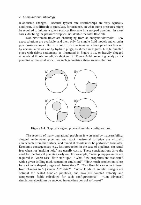
Non-Newtonian flows are challenging from an analysis viewpoint. Fewexact solutions are available, and then, only for simple fluid models and circularpipe cross-sections. But it is not difficult to imagine subsea pipelines blockedby accumulated wax or by hydrate plugs, as shown in Figures 1-1a,b, bundledpipes with debris settlement, as illustrated in Figure 1-1c, or heavily cloggedeccentric drillhole annuli, as depicted in Figure 1-1d, requiring analysis forplanning or remedial work. For such geometries, there are no solutions.
(a) (b)
(c) (d)
Figure 1-1. Typical clogged pipe and annular configurations.
The severity of many operational problems is worsened by inaccessibility:clogged underwater pipelines and stuck horizontal drillpipe are virtuallyunreachable from the surface, and remedial efforts must be performed from afar.Economic consequences, e.g., lost production in the case of pipelines, rig rentalfees when not “making hole,” are usually costly. These considerations drive theneed for rheological planning early on. For example, “What pump pressures arerequired in ‘worst case’ flow start-up?” “What flow properties are associatedwith a given drilling mud, cement, or emulsion?” “How much production is lostfor variously shaped plugs and obstructions?” “Can flow blockage be inferredfrom changes in “Q versus ∆p” data?” “What kinds of annular designs areoptimal for heated bundled pipelines, and how are coupled velocity andtemperature fields calculated for such configurations?” “Can advancedsimulation algorithms be encoded in real-time control software?”
Introduction: Basic Principles 3
Until recently, these questions were academic because flow models for“real world” problems, typified by those in Figure 1-1, were impossible. Notonly were the partial differential equations nonlinear, making their solutionunwieldy, but the geometrical boundaries where “no-slip” velocity conditionsmust be applied were not amenable to simple description. Engineers anddesigners applied questionable analysis methods, e.g., “mean hydraulic radius,”“slot flow,” and so on, to practical problems, often incurring serious error.
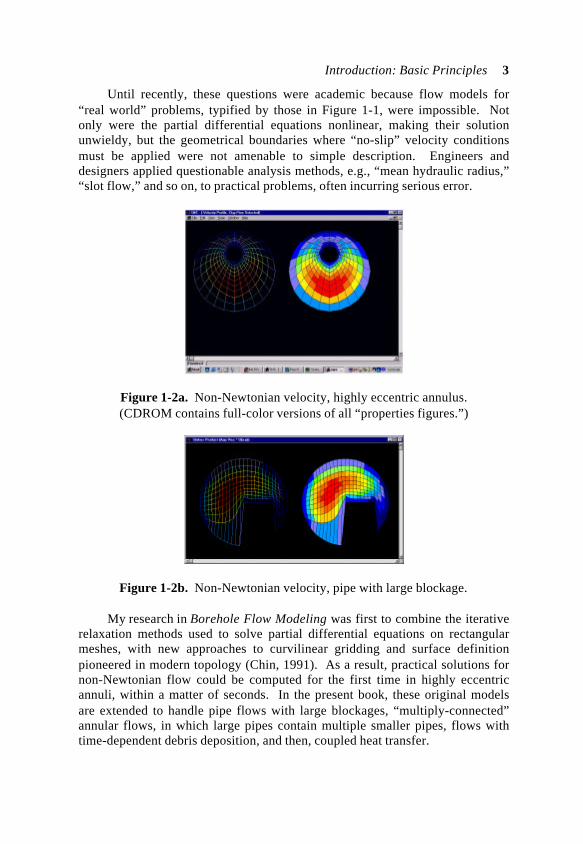
Figure 1-2a. Non-Newtonian velocity, highly eccentric annulus.(CDROM contains full-color versions of all “properties figures.”)
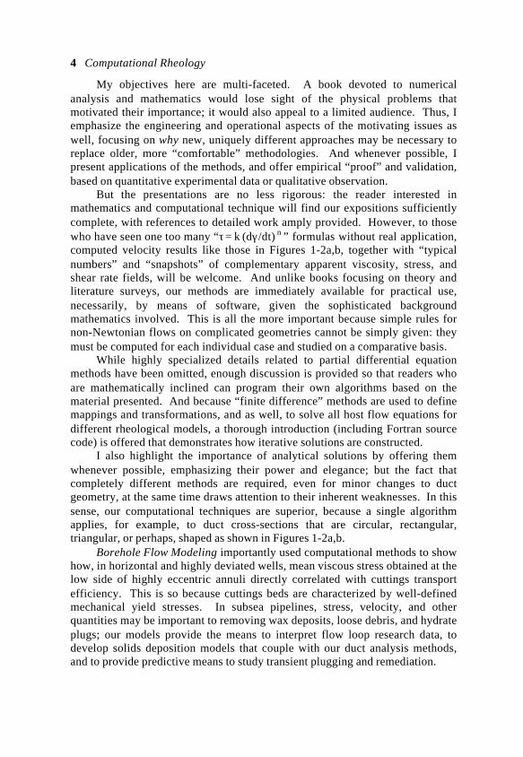
Figure 1-2b. Non-Newtonian velocity, pipe with large blockage.
My research in Borehole Flow Modeling was first to combine the iterativerelaxation methods used to solve partial differential equations on rectangularmeshes, with new approaches to curvilinear gridding and surface definitionpioneered in modern topology (Chin, 1991). As a result, practical solutions fornon-Newtonian flow could be computed for the first time in highly eccentricannuli, within a matter of seconds. In the present book, these original modelsare extended to handle pipe flows with large blockages, “multiply-connected”annular flows, in which large pipes contain multiple smaller pipes, flows withtime-dependent debris deposition, and then, coupled heat transfer.
4 Computational Rheology
My objectives here are multi-faceted. A book devoted to numericalanalysis and mathematics would lose sight of the physical problems thatmotivated their importance; it would also appeal to a limited audience. Thus, Iemphasize the engineering and operational aspects of the motivating issues aswell, focusing on why new, uniquely different approaches may be necessary toreplace older, more “comfortable” methodologies. And whenever possible, Ipresent applications of the methods, and offer empirical “proof” and validation,based on quantitative experimental data or qualitative observation.
But the presentations are no less rigorous: the reader interested inmathematics and computational technique will find our expositions sufficientlycomplete, with references to detailed work amply provided. However, to thosewho have seen one too many “τ = k (dγ /dt)
n ” formulas without real application,
computed velocity results like those in Figures 1-2a,b, together with “typicalnumbers” and “snapshots” of complementary apparent viscosity, stress, andshear rate fields, will be welcome. And unlike books focusing on theory andliterature surveys, our methods are immediately available for practical use,necessarily, by means of software, given the sophisticated backgroundmathematics involved. This is all the more important because simple rules fornon-Newtonian flows on complicated geometries cannot be simply given: theymust be computed for each individual case and studied on a comparative basis.
While highly specialized details related to partial differential equationmethods have been omitted, enough discussion is provided so that readers whoare mathematically inclined can program their own algorithms based on thematerial presented. And because “finite difference” methods are used to definemappings and transformations, and as well, to solve all host flow equations fordifferent rheological models, a thorough introduction (including Fortran sourcecode) is offered that demonstrates how iterative solutions are constructed.
I also highlight the importance of analytical solutions by offering themwhenever possible, emphasizing their power and elegance; but the fact thatcompletely different methods are required, even for minor changes to ductgeometry, at the same time draws attention to their inherent weaknesses. In thissense, our computational techniques are superior, because a single algorithmapplies, for example, to duct cross-sections that are circular, rectangular,triangular, or perhaps, shaped as shown in Figures 1-2a,b.
Borehole Flow Modeling importantly used computational methods to showhow, in horizontal and highly deviated wells, mean viscous stress obtained at thelow side of highly eccentric annuli directly correlated with cuttings transportefficiency. This is so because cuttings beds are characterized by well-definedmechanical yield stresses. In subsea pipelines, stress, velocity, and otherquantities may be important to removing wax deposits, loose debris, and hydrateplugs; our models provide the means to interpret flow loop research data, todevelop solids deposition models that couple with our duct analysis methods,and to provide predictive means to study transient plugging and remediation.
Introduction: Basic Principles 5
WHY STUDY RHEOLOGY?
Many books on rheology develop constitutive equations and kinematicalrelationships, offering illustrations, typically showing flat “small n” velocityprofiles and even flatter “plug flows” characteristic of Bingham plastics. Inpipeline and annular petroleum applications, these are not very useful since theprimary concerns are operational ones that focus on plugging. This book insteaddescribes computer methods for “real world” geometries, and applications toproblems like cuttings transport, sand cleaning, wax deposition, and hydratebuildup. In addition, numerous “color snapshots” of practical flowfields aregiven, not just for velocity, but for apparent viscosity, shear rate, viscous stress,and dissipation function distributions. In several examples, actual “numbers”are given to provide the “physical feel” that engineers need to enhance their“personal” experience with such flows. Also, general results for a number ofdifficult eccentric annular configurations are given for Newtonian flows.
The author believes that a book describing modern theory and numericalmethods has limited value unless software is made available to industry. In thesame vein, software is not very useful unless problem set-up is straightforwardand fast, computations are extremely rapid, and three-dimensional color displaysof all spatially varying quantities are immediately available on solution. This isimperative because engineers use such models not as a means to study rheologyin itself, but as a means to understand problems that plague operationalefficiency. For example, “Does viscous stress correlate with cuttings bedremoval?” “As beds become less ‘cohesive,’ to what extent can velocity-basedcorrelations be used?” “How can existing civil engineering ‘rules of thumb’ beextrapolated to oilfield pipeline dimensions?” “Can the extensions belegitimately made when the rheologies are non-Newtonian?”
I emphasize that while the algorithms are predictive and very efficient,they do have their limitations. In this book, I study steady, laminar flows only,and do not consider turbulence. Also, chemistry and thermodynamics are notconsidered because they are not the focus of this effort. I emphasize the role offluid mechanics as one providing correlation parameters for debris transport andcleaning, and highlight the methods used in developing deposition and erosionmodels. However, the development of models specific to individualapplications is a research endeavor in itself, so that specific models,consequently, are not given. Instead, qualitative results obtained from a numberof client applications are offered to provide the reader with broad exposure tothe potential afforded by computational rheology methods.
Nonetheless, broad usage is possible, even within these constraints. In theliterature, simplifying models have been used to simulate a variety of industryproblems, and it is enlightening to offer at least a partial list of applications:
6 Computational Rheology
• Process design for manufacturing, e.g., heat and melt flow behavior in dies,extruder screws, molds, and so on,
• Industrial manufacturing, e.g., wire coating extrusion, coatings for glassrovings, extrusions, mixing, coating, and injection molding for food andpolymer processing,
• Roller coating of foil and aluminum sheets,
• Modeling power requirements and viscous drag for peanut butter andmayonnaise flows,
• Movement of “mechanically extracted meat” in food processing (after meatis removed from carcasses and bone is separated, it is compressed with“crushers,” ultimately becoming “goo-like” with nonlinear characteristics).
Within the petroleum industry, rheology is important in all aspects ofexploration and production, and also in oilfield development and pipelinetransport. In concluding, we can list numerous applications, among them,
• In drilling vertical wells, cuttings are efficiently removed by increasingvelocity, viscosity, or both, while in horizontal and highly deviated wells,cleaning efficiency correlates with bottom viscous stress in eccentric annuli,
• Flowline debris are transported as “solids in fluid” systems, or alternatively,ground slurries, with rheological considerations entering economicdecisions,
• Efficient cementing and completions require a good understanding ofrheology as it relates to mud displacement and pumping requirements,
• Hydraulic fracturing and stimulation involve proppant transport, withrheology dictating how well a fluid convects solid particulates and howresistant it is to pumping (one less pumping truck in the field can addsignificantly to profit margins!),
• In deep subsea applications, “flow assurance,” i.e., the application ofprevention and remediation techniques, and operating strategies, to possibleflowline blockage, is used to transport crude economically,
• Accurate modeling of wax deposition and hydrate formation, and theirpotential for plugging flowlines, requires coupled solutions with non-Newtonian flow solvers in order to model interacting solids and fluidsflowfields,
• The thermal performance of subsea bundle flowlines, involving the solutionof coupled velocity and temperature fields, requires non-Newtonian flowanalysis in complicated domains, and
• In offshore operations, severe slugging in risers and tiebacks is a majorconcern in the design and operation of deepwater production systems.
Introduction: Basic Principles 7
REVIEW OF ANALYTICAL RESULTS
We have satisfactorily answered “Why study rheology?” In petroleumengineering, we emphasize that “rheology” necessarily implies “computationalrheology,” since operational questions bearing important economic implicationscannot be answered without dealing with measured constitutive relationshipsand actual clogged pipeline and annular borehole geometries. Before delvinginto our subject matter, it is useful to review several closed form solutions.These are useful because they provide important validation points for calculatedresults, and instructive because they show how limiting analytical methods are.For our purposes, I will not list one-dimensional, planar solutions, which havelimited petroleum industry applications, but focus on pipe and annular flows inthis section. Rectangular ducts will be treated later in Chapter 7.
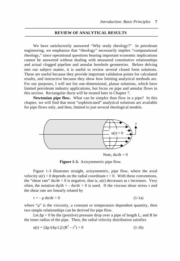
Newtonian pipe flow. What can be simpler than flow in a pipe? In thischapter, we will find that most “sophisticated” analytical solutions are availablefor pipe flows only, and then, limited to just several rheological models.
r
Note, du/dr < 0
u(r) > 0
Figure 1-3. Axisymmetric pipe flow.
Figure 1-3 illustrates straight, axisymmetric, pipe flow, where the axialvelocity u(r) > 0 depends on the radial coordinate r > 0. With these conventions,the “shear rate” du/dr < 0 is negative, that is, u(r) decreases as r increases. Veryoften, the notation dγ/dt = - du/dr > 0 is used. If the viscous shear stress τ andthe shear rate are linearly related by
τ = - µ du/dr > 0 (1-1a)
where “µ” is the viscosity, a constant or temperature dependent quantity, thentwo simple relationships can be derived for pipe flow.
Let ∆p > 0 be the (positive) pressure drop over a pipe of length L, and R bethe inner radius of the pipe. Then, the radial velocity distribution satisfies
u(r) = [∆p /(4µ L)] (R2 – r2) > 0 (1-1b)
8 Computational Rheology
Note that u is constrained by a “no-slip” velocity condition at r = R. If theproduct of “u(r)” and the infinitesimal ring area “2πr dr” is integrated over (0,R),we obtain the volume flow rate expressed by
Q = πR4∆p /(8µ L) > 0 (1-1c)
Equation (1-1c) is the well-known Hagen-Poiseuille formula for flow in apipe. These solutions do not include unsteadiness or compressibility. Theseresults are exact relationships derived from the Navier-Stokes equations, whichgovern viscous flows when the stress-strain relationships take the linear form inEquation 1-1a. We emphasize that the Navier-Stokes equations apply toNewtonian flows only, and not to more general rheological models.
Note that viscous stress (and the wall value τw) can be calculated fromEquation 1-1a, but the following formulas can also be used,
τ (r) = r ∆p/2L > 0 (1-2a)
τw = R ∆p/2L > 0 (1-2b)
Equations 1-2a,b apply generally to steady laminar flows in circular pipes, andimportantly, whether the rheology is Newtonian or not. But they do not apply toducts with other cross-sections, or to annular flows, even concentric ones,whatever the fluid.
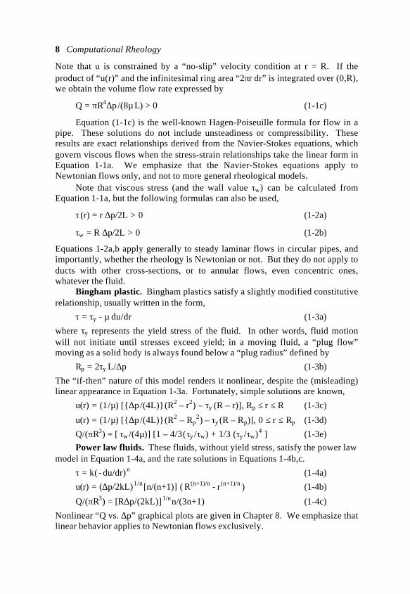
Bingham plastic. Bingham plastics satisfy a slightly modified constitutiverelationship, usually written in the form,
τ = τy - µ du/dr (1-3a)
where τy represents the yield stress of the fluid. In other words, fluid motionwill not initiate until stresses exceed yield; in a moving fluid, a “plug flow”moving as a solid body is always found below a “plug radius” defined by
Rp = 2τy L /∆p (1-3b)
The “if-then” nature of this model renders it nonlinear, despite the (misleading)linear appearance in Equation 1-3a. Fortunately, simple solutions are known,
u(r) = (1 /µ) [∆p /(4L) (R2 – r2) – τy (R – r)], Rp ≤ r ≤ R (1-3c)
u(r) = (1 /µ) [∆p /(4L) (R2 – Rp2) – τy (R – Rp)], 0 ≤ r ≤ Rp (1-3d)
Q/(πR3) = [ τw /(4µ)] [1 – 4/3 (τy /τw) + 1/3 (τy /τw) 4 ] (1-3e)
Power law fluids. These fluids, without yield stress, satisfy the power lawmodel in Equation 1-4a, and the rate solutions in Equations 1-4b,c.
τ = k ( - du/dr) n (1-4a)
u(r) = (∆p/2kL) 1/n
[n/(n+1)] ( R (n+1)/n - r
(n+1)/n ) (1-4b)
Q/(πR3) = [R∆p/(2kL)] 1/n
n/(3n+1) (1-4c)
Nonlinear “Q vs. ∆p” graphical plots are given in Chapter 8. We emphasize thatlinear behavior applies to Newtonian flows exclusively.

Introduction: Basic Principles 9
Newtonian, parabolic profile
Power law, n = 0.5
Power law, n >> 1
Bingham plastic, plug zone
Figure 1-4. Typical non-Newtonian velocity profiles.
Herschel-Bulkley fluids. This model combines power law with yieldstress characteristics, with the result that,
τ = τy + k ( - du/dr) n (1-5a)
u(r) = k -1/n
(∆p/2L) -1
n/(n+1) (1-5b)× [(R∆p/2L - τy)
(n+1)/n - (r∆p/2L - τy) (n+1)/n], Rp ≤ r ≤ R
u(r) = k -1/n
(∆p/2L) -1
n/(n+1) (1-5c)× [(R∆p/2L - τy)
(n+1)/n - (Rp ∆p/2L - τy) (n+1)/n], 0 ≤ r ≤ Rp
Q/(πR3) = k -1/n
(R∆p/2L) -3
(R∆p/2L - τy) (n+1)/n (1-5d)
× [(R∆p/2L - τy)2 n /(3n+1) + 2 τy (R∆p/2L - τy) n /(2n+1) + τy
2 n/(n+1)]
where the plug radius Rp is again defined by Equation 1-3b.
10 Computational Rheology
Ellis fluids. Ellis fluids satisfy a more complicated constitutiverelationship, with the following known results,
τ = - du/dr /(A + B τ α−1) (1-6a)
u(r) = A ∆p (R2 – r2)/(4L) + B(∆p/2L) α ( R
α+1 - r α+1)/(α + 1) (1-6b)
Q/(πR3) = Aτw /4 + B τwα
/(α+3) (1-6c)
= A(R∆p/2L) /4 + B (R∆p/2L) α
/(α+3)
Dozens of additional rheological models appear in the literature, but speciallyrelevant ones will be described later in this book. Typical qualitative features ofthe associated velocity profiles are shown in Figure 1-4.
Annular flow solutions. The only known exact, closed form, analyticalsolution is a classic one describing Newtonian flow in a concentric annulus. LetR be the outer radius, and κR be the inner radius, so that 0 < κ < 1. Then, it canbe shown that,
u(r) = [R2∆p /(4µL)]× [ 1 - (r/R)2 + (1- κ2 ) loge (r/R) / loge (1/κ) ] (1-7a)
Q = [πR4∆p /(8µL)] [ 1 - κ4 - (1- κ2 )2 / loge (1/κ) ] (1-7b)
For non-Newtonian flows, even for concentric geometries, numerical proceduresare required, e.g., see Fredrickson and Bird (1958), Bird, Stewart and Lightfoot(1960), or Skelland (1967). The limited number of exact solutions unfortunatelysummarizes the state-of-the-art, and for this reason, recourse must be made tocomputational rheology for the great majority of practical problems.
Particulate settling. The terminal velocity of particles is important todeposition studies and particulate settling. Because a “well-known” formula isindiscriminately used, it is instructive to point out key assumptions (and hence,restrictions) behind the result. Newton’s law “F = ma” requires that theacceleration d2z/dt2 propelling a mass M must equal the external force F. In thiscase, it consists of the weight “-Mg,” where g is the acceleration due to gravity,the buoyancy force “4/3 πa3ρf g,” where a sphere of radius “a” and a fluid ofdensity ρf are assumed, and finally, a hydrodynamic viscous drag.
Usually, a Newtonian flow is assumed for the latter, and then, in the lowReynolds number limit, for which the laminar drag becomes “6πµaU.” Thisformula also assumes a smooth sphere, and dynamic effects such as “fluttering”are ignored. Even so, the mathematics involved in its derivation is complicated;for non-Newtonian flows, analogous closed form solutions are not available.Terminal velocity is obtained by setting d2z/dt2 = 0 and solving for “U.”Needless to say, the result does not apply to non-Newtonian flows, nor toparticles other than spherical, but given the lack of solutions, the result is usedoften anyway, although sometimes with empirical corrections. Kapfer (1973)provides examples of this common usage.
Introduction: Basic Principles 11
OVERVIEW OF ANNULAR FLOW
Although pipe flows precede annular ones in simplicity, and “ought” to bediscussed in that order, I consider annular flows first because the mappingmethods used in this book were originally developed and empirically validatedfor such applications. Chapters 2-5 describe three recent annular borehole flowmodels, first presented in Borehole Flow Modeling, and now reevaluated withmore physical insight. They were designed to handle the special problems thatarise from drilling and producing deviated and horizontal wells, e.g., cuttingstransport, stuck pipe, cementing and coiled tubing. The models deal with (i)eccentric, nonrotating flow, (ii) concentric rotating flow, and (iii) recirculatingheterogeneous flow. In this section, we introduce the subject of boreholeannular flow, briefly discuss the capabilities of the models, and describeoperational problems that benefit from detailed flow analysis.
The first model allows arbitrary eccentricity, assuming that the pipe (orcasing) does not rotate. It solves the complete nonlinear viscous flow equationson “boundary conforming” grids, and does not invoke the “narrow annulus,”“parallel plate,” “slot flow,” or “hydraulic radius” assumptions commonly used.Holes with washouts, cuttings beds, and square drill collars, for example, areeasily simulated. The model is developed for Newtonian, power law, Binghamplastic, and Herschel-Bulkley fluids.
The second model permits general pipe rotation, but it is restricted toconcentric geometries. For Newtonian fluids, the results are shown to be exactsolutions to the Navier-Stokes equations; both axial and azimuthal velocitiessatisfy no-slip conditions for all diameter ratios. For power law flows, a narrowannulus assumption is invoked that allows us to derive explicit closed formanalytical solutions for all physical quantities. These formulas are easilyprogrammed on pocket calculators. The results are checked with our Newtonianformulas and are consistent with these exact results in the “n=1” limit.
These models assume constant density, unidirectional axial flow whereapplied pressure gradients are exactly balanced by viscous stresses. These flowsform the majority of observed fluid motions. But in deviated wells, especiallywhere drilling mud circulation has been temporarily interrupted, gravitysegregation often causes weighting materials such as barite, fine cuttings, andcement additives to fall out of suspension. The resulting density variations andinertial effects are primarily responsible for the strange “recirculating vortexflows” that have been experimentally observed from time to time. Theseisolated tornado-like clusters, completely fluid-dynamical in origin, aredangerous because they impede the mainstream flow; also, they entrain drilledcuttings, and form stationary obstacles in the annulus.
Recirculating flows are stable packets of angular momentum that arewholly self-contained in a stationary envelope that sits in the midst of an axial
12 Computational Rheology
flow. The latter flow is, effectively, blocked. Within the envelope are rotatingfluid masses, some of which are roped off by closed streamlines; these highlythree-dimensional flows are known to capture and trap solid particles andcuttings. The third model describes these fascinating fluid motions andidentifies the controlling nondimensional parameter. Computer simulationsshowing their generation and growth are given, and ways to avoid or eliminatetheir occurrence are suggested. These recirculating vortices have also beenobserved in pipelines in actual process plant case histories, and are thereforerelevant to flow assurance studies in deep subsea applications.
Although the mathematical models and numerical simulators had beenavailable since 1987, original book publication was withheld until 1991, pendingapplication to field and laboratory examples. Often, the required data andempirical results were either unavailable or proprietary, contributing to delays inthe evaluation of the work. Experimental validation was crucial in establishingthe credibility and accuracy of the computer modeling, especially becauseanalytical solutions simply do not exist for the purposes of verification. Sincenumerical differencing methods, iteration and programming techniquesinvariably introduce additional assumptions that may be unphysical, consistencychecks with empirical results were essential. These extraneous effects includetruncation error, mesh dependence, and numerical viscosity.
Eventually, cuttings transport data, stuck pipe and other complementaryinformation became available, and the desired comparisons were undertakenafter some initial delay. The first applications results were published in a seriesof articles carried by Offshore Magazine beginning in 1990. An expanded“field-oriented” treatment dealing with rigsite applications is offered here inChapter 5. This book explains in detail the mathematical models and numericalalgorithms used, provides calculated examples of “difficult” annular flows, andapplies the computer models to problems related in hole cleaning, stuck pipe,and cementing in deviated and horizontal wells. The extension to coupledvelocity and thermal flowfields, important to analyzing “bundled pipelines” indeep subsea applications, is carried out in Chapter 6.
It is not essential to understand the details of the mathematics in order toappreciate the nuances of annular flow as uncovered by our calculations. Infact, the reader is encouraged to browse through the computed “snapshots” priorto any detailed study. Mathematics aside, the practical implications suggestedby our examples will be understandable to most petroleum engineers. Theexperienced researcher will have little trouble programming the flow modelsderived here. However, practitioners may obtain algorithms from GulfPublishing Company in the form of PC-executable software. Professionalsinterested in source code extensions and more sophisticated versions of theavailable program are encouraged to contact the author directly. All numericalalgorithms are written in standard Fortran, and are readily ported to differenthardware environments. Further software details are offered in Chapter 10.
Introduction: Basic Principles 13
REVIEW OF PRIOR ANNULAR MODELS
Annular flow analysis is important to drilling and production in deviatedand horizontal wells. Different applications will be introduced and covered indetail in Chapter 5. Despite their significance, few rigorous simulation modelsare available for research or field use. There are several reasons for this dearthof analysis. First, the governing equations are nonlinear; this means that anyuseful solutions are necessarily numerical. Second, most practical annulargeometries are complicated, making no-slip velocity boundary conditionsdifficult to enforce with any accuracy. Third, few computational algorithms arepresently available for general rheologies that are stable, fast and robust.
Consequently, researchers have chosen to study simpler although lessrealistic models whose mathematics are at least amenable to solution. Theselimitations have now been overcome, to some extent through technologytransfer from related disciplines. Much of our work on eccentric flow, forexample, represents an extension of aerospace industry research in simulatingannular-like motions in jet engine ducts. Nonlinear equations are solved, forexample, using fast iterative techniques developed by aerodynamicists for shearflows. And the work of Chapter 4 on heterogeneous flows draws, in part, uponthe literature of dynamic meteorology and oceanography.
The model development summarized in this book is self-contained. Thecomplete equations of motion for a fluid having a general stress tensor (Bird,Stewart and Lightfoot, 1960; Schlichting, 1968; Slattery, 1981; Streeter, 1961)are assumed. They are solved using physical boundary conditions relevant topetroleum applications (Gray and Darley, 1980; Moore, 1974; Whittaker, 1985;Quigley and Sifferman, 1990; Govier and Aziz, 1977). The resultingformulations are solved using special relaxation methods and analyticaltechniques. An introduction to these methods may be found in Lapidus andPinder (1982), Crochet et al. (1984), and Thompson et al. (1985). Let us reviewthe existing literature on annular flow, emphasizing that no attempt is made tooffer an exhaustive or comprehensive survey.
Modeling efforts may be classified into several increasingly sophisticatedcategories. For example, the exact solution of Fredrickson and Bird (1958) forpower law fluids is among the simplest; this numerical solution applies toconcentric, nonrotating power law fluids. Eccentric annular flows are morecomplicated, and have been modeled under limiting assumptions. To simplifythe mathematics, authors assume that the annulus is “almost concentric.” This“parallel plate,” “narrow annulus,” or “slot flow” assumption is almost universalin the petroleum literature. But the results of these investigations are appealingbecause they provide a convenient analytical representation of the solution usingelliptic integrals. However, their usefulness is severely limited because feweccentric annuli in deviated wells are nearly concentric.
14 Computational Rheology
Recently, Haciislamoglu and Langlinais (1990) importantly removed thisslot flow restriction by reformulating the governing equations in “bipolarcoordinates.” Just as circular polar coordinates imply simplifications to singlewell radial flow simulation, bipolar coordinates allow exact annular flowmodeling of circular drillpipes and boreholes with arbitrary standoffs. Theauthors used an iterative finite difference method to model Bingham fluids, butthey did not provide information on computing times and numerical stability orcode portability. However, limitations on the mapping used means that themethodology cannot be extended to handle boreholes with cuttings beds andwashouts, or noncircular drillpipes and casings with stabilizers or centralizers.
In a second important paper, Haciislamoglu and Langlinais (1990)correctly pointed out that slot flow approaches simulate radial shear only andneglect that component in the circumferential direction. These models, in otherwords, incorrectly use the equation for narrow concentric flow withoutaccounting for the additional circumferential shear due to eccentricity. Anothercategory of annular models reverts to simpler concentric flows, but allowsconstant speed rotation. Some of these are listed in the references. However,the solution techniques are cumbersome and not amenable for even research use.In Chapter 3, a closed form analytical solution is derived whose results agreewith Savins and Wallick (1966) and Luo and Peden (1989a, 1989b).
THE NEW COMPUTATIONAL MODELS
This book focuses on the annular models conceived in Borehole FlowModeling, and extended since then to include coupled velocity and thermalfields, with significant speed improvements. Also, general methodologies fornon-Newtonian duct flows with arbitrary geometric cross-sections appear inprint for the first time. New algorithms are presented that show how ductsimulation methods can be combined with solids deposition and erosion modelsto describe wax buildup and hydrate formation in deep subsea flowlines.
Eccentric, nonrotating annular flow. The need for fast, stable, andaccurate flow solvers for general eccentric annuli is central to drilling andproduction engineering. Because of mathematical difficulties, i.e., thenonlinearity of the governing equations and the complexity of most geometries,the problem is usually simplified by using unrealistic slot flow assumptions.Even then, the unwieldy elliptic integrals that result shed little physical insightinto what remains of the problem. Moreover, the integrals require intensivecomputations, further decreasing their usefulness in field applications.
In Chapter 2, annular cross-sections containing eccentric circles arepermitted. But importantly, the borehole contour may be modified “point bypoint” to simulate the effects of cuttings beds or wall deformations due toerosion and swelling. The pipe (or casing) contour may be likewise modified,
Introduction: Basic Principles 15
for example, to model square drill collars or stabilizers and centralizers. Narrowannulus and slot flow assumptions are not invoked. The analysis model handlesNewtonian, power law, Bingham plastic, and Herschel-Bulkley fluids. In allcases, the formulation satisfies “no-slip” velocity boundary conditions exactly atall solid surfaces. Since the appearance of Borehole Flow Modeling,underbalanced drilling has gained in popularity. Changes in algorithm designnow permit the modeling of “velocity slip,” crucial modeling foam-based muds.
Our model is derived from first principles using the exact equations ofcontinuum mechanics. These equations are written in coordinates natural to theannular geometry considered. Then second-order accurate solutions for theaxial velocity field, shear rate, shear stress, apparent viscosity, Stokes product,and dissipation function are obtained. These solutions make use of recentdevelopments in boundary conforming grid generation, e.g., Thompson et al.(1985) and relaxation methods (Lapidus and Pinder, 1982; Crochet et al., 1984).
Special graphics software allows computed results to be overlaid on theannular geometry itself, so that physical trends can be visually correlated withposition. The unconditionally stable iteration process requires ten seconds ontypical Pentium class personal computers. Efficient coding allows theexecutable code to reside in less than 100K RAM. One organization, in fact, hasincorporated both mapping and flow solvers successfully in real-time controlsoftware. Note that the Fortran code is portable and compatible with allmachine environments. The computer program, now Windows-based, is writtenfor generalists and uses “plain English” menus requiring only the experience ofnovice petroleum engineers. Graphics capabilities have been significantlyupgraded, and are described in Chapter 6.
The only restriction is our assumption of a stationary nonrotating pipe.This is not overly severe in field applications, since the intended application ofthe model was anticipated in horizontal turbodrilled wells. Also, rotationaleffects will not be important when the tangential pipe speed is small comparedto the average axial speed; for such problems, estimates are easily obtainedusing the dynamic model of Chapter 3.
Eccentric annuli with thermal effects. In deep subsea production, heatedpipelines are sometimes carried within larger pipes containing crude. Heat isnecessary to prevent wax deposition and hydrate formation. Unlike the velocitysimulations above, where fluid attributes like “n” and “k” are constant, theseproperties now depend on temperature, which itself satisfies a thermal boundaryvalue problem dictated by the heating line and ocean environment. Chapter 6extends our methodology to such flows, and illustrative calculations areperformed, showing the differences that arise for two “bundled” geometries.
Concentric, rotating annular flow. Rotational effects are importantwhen drilling at low flow rates, or when rotating the casing during cementing.For eccentric annuli, all three velocity components will be nonlinearly coupled.Although numerical simulation is possible, the simultaneous solution of three
16 Computational Rheology
velocity equations requires computing resources not usually available at userlocations. For this reason, the eccentric model of Chapter 2 is restricted to zerorotation. Constant speed rotation, by contrast, can be treated quite generally forconcentric annuli. However, the usual solution techniques do not lendthemselves to simple use; the final equations are implicit and require iteration.
In Chapter 3, the restriction to power law fluids in narrow annuli is made.Then a simple but powerful application of the Mean Value Theorem ofdifferential calculus allows us to derive closed form solutions for the relativelycomplicated problem. Note that the resulting problem still contains four coupledno-slip conditions, two for each of the axial and circumferential velocities. Thesolutions are shown to be consistent with an exact solution of the Navier-Stokesequations for Newtonian flow, which does not bear any limiting geometricrestrictions. Formulas for apparent viscosity, stress, deformation and dissipationfunction versus “r” are given. The solutions are explicit in that they require noiteration. A Fortran graphics algorithm is also described that conveniently plotsand tabulates desired solutions, without requiring additional investment ingraphical software and hardware.
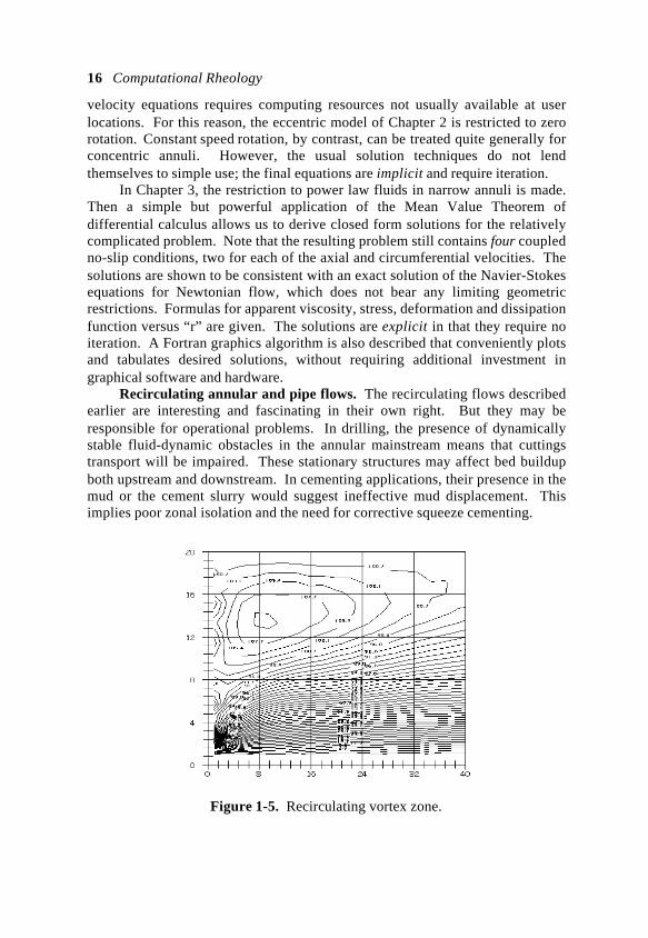
Recirculating annular and pipe flows. The recirculating flows describedearlier are interesting and fascinating in their own right. But they may beresponsible for operational problems. In drilling, the presence of dynamicallystable fluid-dynamic obstacles in the annular mainstream means that cuttingstransport will be impaired. These stationary structures may affect bed buildupboth upstream and downstream. In cementing applications, their presence in themud or the cement slurry would suggest ineffective mud displacement. Thisimplies poor zonal isolation and the need for corrective squeeze cementing.
Figure 1-5. Recirculating vortex zone.
Introduction: Basic Principles 17
These vortex structures have recently been identified in pipelines inprocess plant applications. In one published study, the recirculation zoneentrained abrasive particles that eroded to pipe over time. Originally, engineersspeculated that high streamwise velocities were to blame; however, subsequentanalysis clearly showed that recirculation was the culprit. In any event, thetransverse extent of any recirculation bubbles likely to be present is the ultimatesolution sought. Thus, the model presented in Chapter 4 solves for streamlineshapes and boundaries. Velocities, stresses, and pressures can in principle beobtained from streamline patterns. The fractional blockage inferred from thepresence of any closed streamlines provides a qualitative danger indicator forcuttings removal and cement displacement.
Duct flows with arbitrary geometries. The second half of this book isdevoted to non-Newtonian pipe flow: not “simple” flows, e.g., Equations 1-1 to1-6, but flows with significant clogging. Our focus is practical, dwelling on “Qvs. ∆p” relationships for pipe clogs typical of wax deposition and hydrateformation. Such results are especially relevant to “start-up” requirements, whenpipelines have stopped production temporarily and fluids have gelled. As withannular flow, we again calculate detailed spatial flowfields withoutapproximation, except to the extent that our flow equations are discretized andsolved using finite difference methods. Exact no-slip conditions are again used,and quantities like apparent viscosity, shear rate, viscous stress, and dissipationfunction, are obtained by post-processing the calculated velocity field. The newduct simulator is described in detail in Chapter 7, and applications to waxdeposition, hydrate growth, and erosion by the convected flow, are developed inChapter 8. Additional advanced topics are covered in Chapters 9 and 10.
PRACTICAL APPLICATIONS
We introduce some practical applications for the annular flow simulatorsdeveloped in Chapters 2, 3, and 4, and also the pipe flow simulator described inChapter 7. These field applications are listed and briefly discussed.
Cuttings transport in deviated wells. The most important operationalproblem confronting drillers of deviated and horizontal wells is cuttingstransport and bed formation. Many excellent experimental studies have beenperformed by industry and university groups, but the results are often confusing.For example, take eccentric inclined annular flows. Velocity, which plays animportant role in vertical holes, has little value as a correlation parameter
beyond 30o deviation. But mean viscous stress turns out to be the parameter ofsignificance; the right threshold value will erode cuttings beds formed at thebottom of highly eccentric annuli. Extensive field data and computationalresults support this view in Chapter 5.
18 Computational Rheology
What role do rotational viscometer measurements taken at the surface playin downhole applications? None, because downhole shear rates, which changefrom case to case, are not known a priori. Or consider pipe rotation. It turnsout that concentric Newtonian flows, often used as the basis for convenientexperiments, have no bearing on real world problems. In this singular limit,both the axial and azimuthal velocities decouple dynamically, and experimentalobservations cannot be extrapolated to other situations.
Spotting fluids and stuck pipe. A related problem is the severe onedealing with stuck pipe. Typically, spotting fluids are used in combination withmechanical jarring motions to free immobile pipe. These impulsive transientflows can also be approximately analyzed since the acceleration and pressuregradient terms in the momentum equation have like physical dimensions. Whatparameter governs spotting fluid effectiveness? How is that quantity related tolubricity? These questions are also addressed in Chapter 5.
Coiled tubing return flow. Sands and fines are often produced in flowingwells. They are removed by injecting non-Newtonian foams delivered by coiledtubing forced into the well. The debris is then transported up the return annulusinside the production tubing, a process not unlike the movement of drilledcuttings. Here, the weight and small diameter of the metal tubing (typically, 1 to2 inches, O.D.) render the annular geometry highly eccentric. This problem isalso suited to the model of Chapter 2.
Cementing. Proper primary cementing creates the fluid seals needed toproduce formation fluids properly. Improper procedures often lead toexpensive, difficult squeeze cementing jobs. Mud that remains in the hole oftendoes so because the cement velocity profile is hydrodynamically unstable,admitting viscous fingering and laminar flow breakdown. How are stablevelocity profiles selected? How are dangerous “recirculation zones” that impedeeffective mud displacement eliminated? How does casing rotation alter the stateof stress in the mud? These questions are addressed in Chapters 2-5.
Improved well planning. Well planning involves mud pump selectionand drilling fluid properties calculations. In vertical wells with concentricannuli, these are straightforward. But simple questions require complicatedanswers for eccentric annular spaces, and particularly when they contain non-Newtonian fluids. “Can the pump operate through a range of mud weights andflow rates for a long horizontal well?” The dependence of flow rate on pressuregradient, of course, is nonlinear; and just as problematic is the apparent viscositydistribution, which depends on pressure gradient as well as annular geometry.
Borehole stability. Borehole stability depends on several factors,principally mud chemistry and elastic states of stress. But annular flow can beimportant. For example, rapid velocities or surface stresses can erode boreholewalls and promote washouts in unconsolidated sands. Drilling muds may alsoprove abrasive since they carry drilled cuttings that impinge into the formation.
Introduction: Basic Principles 19
Wellbore heat generation. Temperature effects can be important indrilling. While heat generation due to internal friction is small, overalltemperature increases in a closed system may be significant for large circulationtimes. These may affect the thermal stability and thinning of oil-base muds.Heat generation may be important to temperature log interpretation. Tocalculate formation temperature correctly from measurements obtained whiledrilling, it is necessary to correct for the component of temperature due to totalcirculation time and the rheological effects of the drilling fluid used.
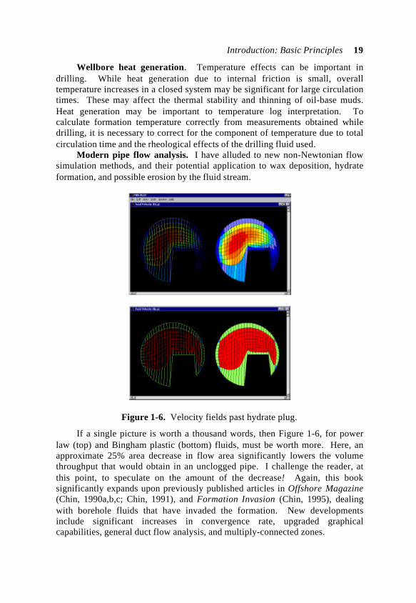
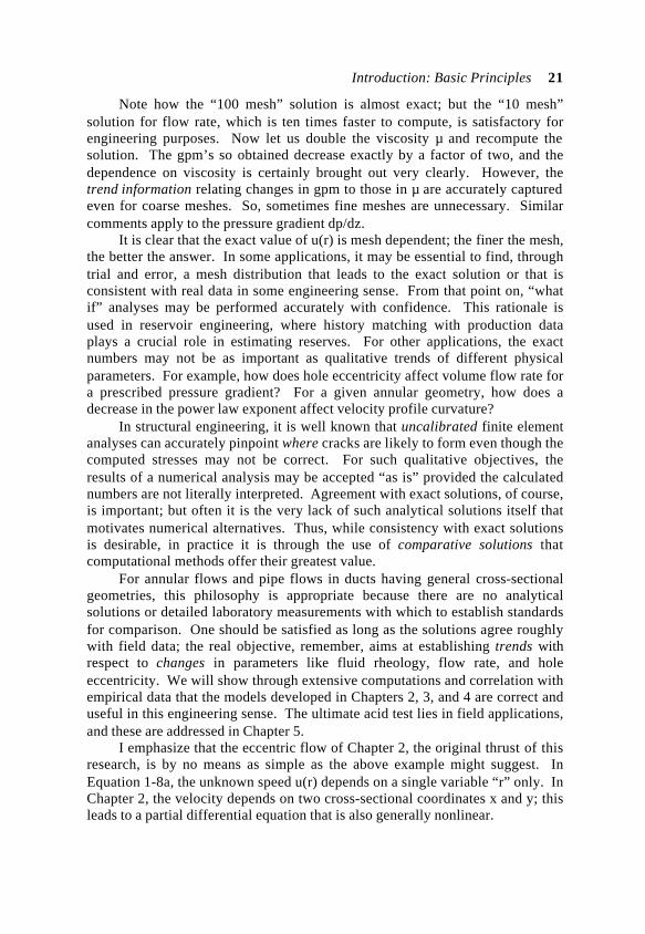
Modern pipe flow analysis. I have alluded to new non-Newtonian flowsimulation methods, and their potential application to wax deposition, hydrateformation, and possible erosion by the fluid stream.
Figure 1-6. Velocity fields past hydrate plug.
If a single picture is worth a thousand words, then Figure 1-6, for powerlaw (top) and Bingham plastic (bottom) fluids, must be worth more. Here, anapproximate 25% area decrease in flow area significantly lowers the volumethroughput that would obtain in an unclogged pipe. I challenge the reader, atthis point, to speculate on the amount of the decrease! Again, this booksignificantly expands upon previously published articles in Offshore Magazine(Chin, 1990a,b,c; Chin, 1991), and Formation Invasion (Chin, 1995), dealingwith borehole fluids that have invaded the formation. New developmentsinclude significant increases in convergence rate, upgraded graphicalcapabilities, general duct flow analysis, and multiply-connected zones.
20 Computational Rheology
PHILOSOPHY OF NUMERICAL MODELING
Reservoir engineers and structural dynamicists, for example, routinely useadvanced finite difference and finite element methods. But drillers havetraditionally relied upon simpler handbook formulas and tables that areconvenient at the rigsite. Simulation methods are powerful, to be sure, but theyhave their limitations. This section explains the pitfalls and the philosophy onemust adopt in order to bring state-of-the-art techniques to the field. Importantly,we emphasize that numerical methods do not always yield exact answers. Butmore often than not, they produce excellent trend information that is useful inpractical application. For our purposes, consider the steady, concentric annularflow of a Newtonian fluid (Bird et al., 1960). The governing equations are
d2u(r)/dr2 + r-1 du/dr = (1/µ) dp/dz (1-8a)
u(Ri) = u(Ro) = 0 (1-8b)
In Equations 1-8a,b, u(r) is the annular speed satisfying no-slip conditions at theinner and outer radii, Ri and Ro. Here, the viscosity µ and the applied pressure
gradient dp/dz are known constants. The exact solution was given earlier.Let us examine the consequences of a numerical solution. A “second-order
accurate” scheme is derived by “central differencing” Equation 1-8a as follows,
(uj-1 -2uj +uj+1) /(∆r)2 + (uj+1 -uj-1)/2rj∆r = (1/µ) dp/dz (1-9a)
where uj refers to u(r) at the jth radial node at the rj location, j being an ordering
index. Equation 1-9a can be evaluated at any number of interior nodes for themesh length ∆r. The resulting difference equations, when augmented by
u1 = ujmax = 0 (1-9b,c)
using Equation 1-8b, form a tridiagonal system of jmax unknowns that lends
itself to simple solution for uj and its total volume flow rate. For our first run,
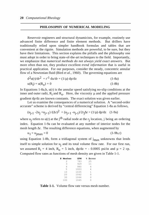
we assumed Ri = 4 inch, Ro = 5 inch, dp/dz = - 0.0005 psi/in and µ = 2 cp.
Computed flow rates as functions of mesh density are given in Table 1-1. # Meshes GPM % Error 2 783 25 3 929 11 4 980 6 5 1003 4 10 1035 1 20 1042 0 30 1044 0 100 1045 0
Table 1-1. Volume flow rate versus mesh number.
Introduction: Basic Principles 21
Note how the “100 mesh” solution is almost exact; but the “10 mesh”solution for flow rate, which is ten times faster to compute, is satisfactory forengineering purposes. Now let us double the viscosity µ and recompute thesolution. The gpm’s so obtained decrease exactly by a factor of two, and thedependence on viscosity is certainly brought out very clearly. However, thetrend information relating changes in gpm to those in µ are accurately capturedeven for coarse meshes. So, sometimes fine meshes are unnecessary. Similarcomments apply to the pressure gradient dp/dz.
It is clear that the exact value of u(r) is mesh dependent; the finer the mesh,the better the answer. In some applications, it may be essential to find, throughtrial and error, a mesh distribution that leads to the exact solution or that isconsistent with real data in some engineering sense. From that point on, “whatif” analyses may be performed accurately with confidence. This rationale isused in reservoir engineering, where history matching with production dataplays a crucial role in estimating reserves. For other applications, the exactnumbers may not be as important as qualitative trends of different physicalparameters. For example, how does hole eccentricity affect volume flow rate fora prescribed pressure gradient? For a given annular geometry, how does adecrease in the power law exponent affect velocity profile curvature?
In structural engineering, it is well known that uncalibrated finite elementanalyses can accurately pinpoint where cracks are likely to form even though thecomputed stresses may not be correct. For such qualitative objectives, theresults of a numerical analysis may be accepted “as is” provided the calculatednumbers are not literally interpreted. Agreement with exact solutions, of course,is important; but often it is the very lack of such analytical solutions itself thatmotivates numerical alternatives. Thus, while consistency with exact solutionsis desirable, in practice it is through the use of comparative solutions thatcomputational methods offer their greatest value.
For annular flows and pipe flows in ducts having general cross-sectionalgeometries, this philosophy is appropriate because there are no analyticalsolutions or detailed laboratory measurements with which to establish standardsfor comparison. One should be satisfied as long as the solutions agree roughlywith field data; the real objective, remember, aims at establishing trends withrespect to changes in parameters like fluid rheology, flow rate, and holeeccentricity. We will show through extensive computations and correlation withempirical data that the models developed in Chapters 2, 3, and 4 are correct anduseful in this engineering sense. The ultimate acid test lies in field applications,and these are addressed in Chapter 5.
I emphasize that the eccentric flow of Chapter 2, the original thrust of thisresearch, is by no means as simple as the above example might suggest. InEquation 1-8a, the unknown speed u(r) depends on a single variable “r” only. InChapter 2, the velocity depends on two cross-sectional coordinates x and y; thisleads to a partial differential equation that is also generally nonlinear.
22 Computational Rheology
The “two-point” boundary conditions in Equation 1-8b are thereforereplaced by no-slip velocity conditions enforced along two general arbitrarycurves representing the borehole and pipe contours. To implement these no-slipconditions accurately, “boundary conforming meshes” must be used that providehigh resolution in tight spaces. To be numerically efficient, these meshes mustbe variable with respect to all coordinate directions. The difference equationssolved on such host meshes must be solved iteratively; for unlike Equations 1-9a,b,c, which apply to Newtonian flows with constant viscosities, the power law,Bingham plastic, and Herschel-Bulkley fluids considered in this book satisfynonlinear equations with problem-dependent apparent viscosities. Thealgorithms must be fast, stable, and robust; they must produce solutions withoutstraining computing resources. Finally, computed solutions must be physicallycorrect; this is the final arbiter that challenges all numerical simulations.
REFERENCES
Bird, R.B., Stewart, W.E., and Lightfoot, E.N., Transport Phenomena, JohnWiley and Sons, New York, 1960.
Chin, W.C., “Advances in Annular Borehole Flow Modeling,” OffshoreMagazine, February 1990, pp. 31-37.
Chin, W.C., “Exact Cuttings Transport Correlations Developed for High AngleWells,” Offshore Magazine, May 1990, pp. 67-70.
Chin, W.C., “Annular Flow Model Explains Conoco’s Borehole CleaningSuccess,” Offshore Magazine, October 1990, pp. 41-42.
Chin, W.C., “Model Offers Insight into Spotting Fluid Performance,” OffshoreMagazine, February 1991, pp. 32-33.
Chin, W.C., Borehole Flow Modeling in Horizontal, Deviated, and VerticalWells, Gulf Publishing Company, Houston, Texas, 1992.
Chin, W.C., “Eccentric Annular Flow Modeling for Highly DeviatedBoreholes,” Offshore Magazine, Aug. 1993.
Chin, W.C., Formation Invasion, with Applications to Measurement-While-Drilling, Time Lapse Analysis, and Formation Damage, Gulf PublishingCompany, Houston, Texas, 1995.
Crochet, M.J., Davies, A.R., and Walters, K., Numerical Simulation of Non-Newtonian Flow, Elsevier Science Publishers B.V., Amsterdam, 1984.
Davis, C.V., and Sorensen, K.E., Handbook of Applied Hydraulics, McGraw-Hill, New York, 1969.
Introduction: Basic Principles 23
Fredrickson, A.G., and Bird, R.B., “Non-Newtonian Flow in Annuli,” Ind. Eng.Chem., Vol. 50, 1958, p. 347.
Govier, G.W., and Aziz, K., The Flow of Complex Mixtures in Pipes, RobertKrieger Publishing, New York, 1977.
Gray, G.R., and Darley, H.C.H., Composition and Properties of Oil WellDrilling Fluids, Gulf Publishing Company, Houston, 1980.
Haciislamoglu, M., and Langlinais, J., “Non-Newtonian Fluid Flow inEccentric Annuli,” 1990 ASME Energy Resources Conference andExhibition, New Orleans, January 14-18, 1990.
Haciislamoglu, M., and Langlinais, J., “Discussion of Flow of a Power-LawFluid in an Eccentric Annulus,” SPE Drilling Engineering, March 1990, p. 95.
Iyoho, A.W., and Azar, J.J., “An Accurate Slot-Flow Model for Non-NewtonianFluid Flow Through Eccentric Annuli,” Society of Petroleum Engineers Journal,October 1981, pp. 565-572.
King, R.C., and Crocker, S., Piping Handbook, McGraw-Hill, New York, 1973.
Langlinais, J.P., Bourgoyne, A.T., and Holden, W.R., “Frictional PressureLosses for the Flow of Drilling Mud and Mud/Gas Mixtures,” SPE Paper No.11993, 58th Annual Technical Conference and Exhibition of the Society ofPetroleum Engineers, San Francisco, October 5-8, 1983.
Lapidus, L., and Pinder, G., Numerical Solution of Partial DifferentialEquations in Science and Engineering, John Wiley and Sons, New York, 1982.
Luo, Y., and Peden, J.M., “Flow of Drilling Fluids Through Eccentric Annuli,”Paper No. 16692, SPE Annual Technical Conference and Exhibition, Dallas,September 27-3, 1987.
Luo, Y., and Peden, J.M., “Laminar Annular Helical Flow of Power LawFluids, Part I: Various Profiles and Axial Flow Rates,” SPE Paper No. 020304,December 1989.
Luo, Y., and Peden, J.M., “Reduction of Annular Friction Pressure Drop Causedby Drillpipe Rotation,” SPE Paper No. 020305, December 1989.
Moore, P. L., Drilling Practices Manual, PennWell Books, Tulsa, 1974.
Perry, R.H., and Chilton, C.H., Chemical Engineer’s Handbook, McGraw-Hill,New York, 1973.
Quigley, M.S., and Sifferman, T.R., “Unit Provides Dynamic Evaluation ofDrilling Fluid Properties,” World Oil, January 1990, pp. 43-48.
Savins, J.G., “Generalized Newtonian (Pseudoplastic) Flow in Stationary Pipesand Annuli,” Petroleum Transactions, AIME, Vol. 213, 1958, pp. 325-332.
24 Computational Rheology
Savins, J.G., and Wallick, G.C., “Viscosity Profiles, Discharge Rates, Pressures,and Torques for a Rheologically Complex Fluid in a Helical Flow,” A.I.Ch.E.Journal, Vol. 12, No. 2, March 1966, pp. 357-363.
Schlichting, H., Boundary Layer Theory, McGraw-Hill, New York, 1968.
Skelland, A.H.P., Non-Newtonian Flow and Heat Transfer, John Wiley & Sons,New York, 1967.
Slattery, J.C., Momentum, Energy, and Mass Transfer in Continua, Robert E.Krieger Publishing Company, New York, 1981.
Streeter, V.L., Handbook of Fluid Mechanics, McGraw-Hill, New York, 1961.
Thompson, J.F., Warsi, Z.U.A., and Mastin, C.W., Numerical Grid Generation,Elsevier Science Publishing, New York, 1985.
Uner, D., Ozgen, C., and Tosun, I., “Flow of a Power Law Fluid in anEccentric Annulus,” SPE Drilling Engineering, September 1989, pp. 269-272.
Vaughn, R.D., “Axial Laminar Flow of Non-Newtonian Fluids in NarrowEccentric Annuli,” Society of Petroleum Engineers Journal, December 1965, pp.277-280.
Whittaker, A., Theory and Application of Drilling Fluid Hydraulics, IHRDCPress, Boston, 1985.
Yih, C.S., Fluid Mechanics, McGraw-Hill, New York, 1969.
Zamora, M., and Lord, D.L., “Practical Analysis of Drilling Mud Flow in Pipesand Annuli,” SPE Paper No. 4976, 49th Annual Technical Conference andExhibition of the Society of Petroleum Engineers, Houston, October 6-9, 1974.
25
2
Eccentric, Nonrotating, Annular Flow
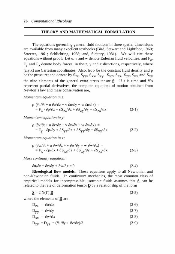
Numerical solutions for the nonlinear, two-dimensional axial velocity field,and its corresponding stress and shear rate distributions, are obtained foreccentric annular flow in an inclined borehole. The homogeneous fluid isassumed to be flowing unidirectionally in a wellbore containing a nonrotatingdrillstring. The unconditionally stable algorithm used draws upon finitedifference relaxation methods (Lapidus and Pinder, 1982; and Crochet, Daviesand Walters, 1984), and contemporary methods in differential geometry andboundary conforming grid generation (Thompson, Warsi and Mastin, 1985).
Slot flow, narrow annulus, and parallel plate assumptions are not invoked.The cross-section may contain conventional concentric or nonconcentric circulardrillpipes and boreholes. But importantly, the hole and pipe contours may bearbitrarily modified “point by point” to simulate the effects of square drillcollars, centralizers, stabilizers, thick cuttings beds, washouts, and general sidewall deformations due to swelling and erosion. “Equivalent hydraulic radii”approximations are never used.
The overall formulation, which applies to general rheologies, is specializedto Newtonian flows, power law fluids, Bingham plastics, and Herschel-Bulkleyflows. In all instances, no-slip velocity boundary conditions are satisfied exactlyat all solid surfaces. Detailed spatial solutions and cross-sectional plots for localannular velocity, apparent viscosity, two components each of viscous stress andshear rate, Stokes product and heat generation due to fluid friction, are presentedfor a large number of annular geometries. Net volume flow rates are also given.
Calculated results are displayed using a special “character-based” textgraphics program that overlays computed quantities on the annular cross-sectionitself, thus facilitating the physical interpretation and visual correlation ofnumerical quantities with annular position. For most annular geometries ofpractical interest, mesh generation requires approximately five seconds ofcomputing time on Pentium machines. Once the host mesh is available, anynumber of “what if” scenarios for differing rheologies or net flow rates can beefficiently evaluated, these simulations again requiring five seconds. Thischapter derives the basic ideas from first principles and explains themmathematically. However, the reader who is more interested in practicalapplications may, without loss of continuity, proceed directly to those sections.
26 Computational Rheology
THEORY AND MATHEMATICAL FORMULATION
The equations governing general fluid motions in three spatial dimensionsare available from many excellent textbooks (Bird, Stewart and Lightfoot, 1960;Streeter, 1961; Schlichting, 1968; and, Slattery, 1981). We will cite theseequations without proof. Let u, v and w denote Eulerian fluid velocities, and Fz,
Fy and Fx denote body forces, in the z, y and x directions, respectively, where
(z,y,x) are Cartesian coordinates. Also, let ρ be the constant fluid density and pbe the pressure; and denote by Szz, Syy, Sxx, Szy, Syz, Sxz, Szx, Syx and Sxythe nine elements of the general extra stress tensor S. If t is time and ∂’srepresent partial derivatives, the complete equations of motion obtained fromNewton’s law and mass conservation are,
Momentum equation in z:
ρ (∂u/∂t + u ∂u/∂z + v ∂u/∂y + w ∂u/∂x) = = Fz - ∂p/∂z + ∂Szz/∂z + ∂Szy/∂y + ∂Szx/∂x (2-1)
Momentum equation in y:
ρ (∂v/∂t + u ∂v/∂z + v ∂v/∂y + w ∂v/∂x) = = Fy - ∂p/∂y + ∂Syz/∂z + ∂Syy/∂y + ∂Syx/∂x (2-2)
Momentum equation in x:
ρ (∂w/∂t + u ∂w/∂z + v ∂w/∂y + w ∂w/∂x) = = Fx - ∂p/∂x + ∂Sxz/∂z + ∂Sxy/∂y + ∂Sxx/∂x (2-3)
Mass continuity equation:
∂u/∂z + ∂v/∂y + ∂w/∂x = 0 (2-4)
Rheological flow models. These equations apply to all Newtonian andnon-Newtonian fluids. In continuum mechanics, the most common class ofempirical models for incompressible, isotropic fluids assumes that S can berelated to the rate of deformation tensor D by a relationship of the form
S = 2 N(Γ) D (2-5)
where the elements of D are
Dzz = ∂u/∂z (2-6)
Dyy = ∂v/∂y (2-7)
Dxx = ∂w/∂x (2-8)
Dzy = Dyz = (∂u/∂y + ∂v/∂z)/2 (2-9)
Eccentric, Nonrotating, Annular Flow 27
Dzx = Dxz = (∂u/∂x + ∂w/∂z)/2 (2-10)
Dyx = Dxy = (∂v/∂x + ∂w/∂y)/2 (2-11)
In Equation 2-5, N(Γ) is the “apparent viscosity” satisfying
N(Γ) > 0 (2-12)
Γ(z,y,x) being a scalar functional of u, v and w defined by the tensor operation
Γ = 2 trace (D•D) 1/2 (2-13)
Unlike the constant laminar viscosity in classical Newtonian flow, theapparent viscosity depends on the details of the particular problem beingconsidered, e.g., the rheological model used, the exact annular geometryoccupied by the fluid, the applied pressure gradient or the net volume flow rate.Also, it varies with the position (z,y,x) in the annular domain. Thus, singlemeasurements obtained from viscometers may not be meaningful in practice.
Power law fluids. These considerations are general. To fix ideas, weexamine one important and practical simplification. The Ostwald-de Waelemodel for two-parameter “power law” fluids assumes that
N(Γ) = k Γn-1 (2-14a)
where the “consistency factor” k and the “fluid exponent” n are constants. Suchpower law fluids are “pseudoplastic” when 0 < n < 1, Newtonian when n = 1,and “dilatant” when n > 1. Most drilling fluids are pseudoplastic. In the limit(n=1, k=µ), Equation 2-14a reduces to the Newtonian model with N(Γ) = µ,where µ is the constant laminar viscosity; in this classical limit, stress is directlyproportional to the rate of strain. Only for Newtonian flows is total volume flowrate a linear function of applied pressure gradient.
Yield stresses. Power law and Newtonian fluids respond instantaneouslyto applied pressure and stress. But if the fluid behaves as a rigid solid until thenet applied stresses have exceeded some known critical yield value, say Syield,then Equation 2-14a can be generalized by writing
N(Γ) = k Γn-1 + Syield/Γ if 1/2 trace (S•S)1/2 > Syield
D = 0 if 1/2 trace (S•S)1/2 < Syield (2-14b)
In this form, Equation 2-14b rigorously describes the general Herschel-Bulkley fluid. When the limit (n=1, k=µ) is taken, the first equation becomes
N(Γ) = µ + Syield/Γ if 1/2 trace (S•S)1/2 > Syield (2-14c)
This is the Bingham plastic model, where µ is now the “plastic viscosity.”Annular flows containing fluids with nonzero yield stresses are more difficult toanalyze, both mathematically and numerically, than those marked by zero yield.
28 Computational Rheology
This is so because there may co-exist “dead” (or “plug”) and “shear” flowregimes with internal boundaries that must be determined as part of the solution.Even though “n = 1,” Bingham fluid flows are essentially nonlinear.
For now, we restrict our discussion to Newtonian and power law flows,that is, to fluids without yield stresses. For flows whose velocities do notdepend on the axial coordinate z, and which further satisfy v = w = 0, thefunctional Γ in Equation 2-14a takes the form
Γ = [ (∂u/∂y)2 + (∂u/∂x)2 ]1/2 (2-15)
so that Equation 2-14a becomes
N(Γ) = k [ (∂u/∂y)2 + (∂u/∂x)2 ](n-1)/2 (2-16)
The apparent viscosity reduces to the conventional “N(Γ) = k (∂u/∂y)(n-1) ”formula for one-dimensional, parallel plate flows considered in the literature.
When both independent variables y and x for the cross-section are present,as in the case for eccentric annular flow, significant mathematical difficultyarises. For one, the ordinary differential equation for annular velocity in simpleconcentric geometries becomes a partial differential equation (PDE). Andwhereas the former requires boundary conditions at two points, the PDE requiresno-slip boundary conditions along two arbitrarily closed curves. Thenonlinearity of the governing PDE and the irregular annular geometry onlycompound these difficulties.
Borehole configuration. The configuration considered is shown in Figure2-1. A drillpipe (or casing) and borehole combination is inclined at an angle αrelative to the ground, with α = 0o for horizontal and α = 90o for vertical wells.Here “z” denotes any point within the annular fluid; Section “AA” is a cut takennormal to the local z axis. Figure 2-2 resolves the vertical body force due togravity at “z” into components parallel and perpendicular to the axis. Figure 2-3provides a detailed picture of the annular cross-section at Section “AA.”
Now specialize the above equations to downhole flows. In Figures 2-1, 2,and 3, we have aligned z, which increases downward, with the axis of the
borehole. The axis may be inclined, varying from α = 0o for horizontal to 90o
for vertical holes. The plane of the variables (y,x) is perpendicular to the z-axis,and (z,y,x) are mutually orthogonal Cartesian coordinates. The body forces dueto the gravitational acceleration g can be resolved into components
Fz = ρ g sin α (2-17)
Fx = - ρ g cos α (2-18)
Fy = 0 (2-19)
If we now assume that the drillpipe does not rotate, the resulting flow canonly move in a direction parallel to the borehole axis. This requires that thevelocities v and w vanish. Therefore,
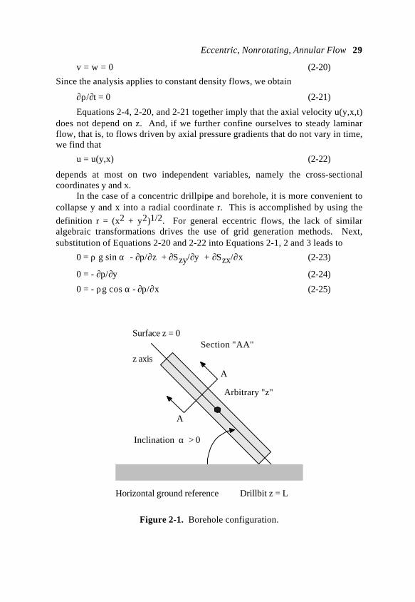
Eccentric, Nonrotating, Annular Flow 29
v = w = 0 (2-20)
Since the analysis applies to constant density flows, we obtain
∂ρ/∂t = 0 (2-21)
Equations 2-4, 2-20, and 2-21 together imply that the axial velocity u(y,x,t)does not depend on z. And, if we further confine ourselves to steady laminarflow, that is, to flows driven by axial pressure gradients that do not vary in time,we find that
u = u(y,x) (2-22)
depends at most on two independent variables, namely the cross-sectionalcoordinates y and x.
In the case of a concentric drillpipe and borehole, it is more convenient tocollapse y and x into a radial coordinate r. This is accomplished by using the
definition r = (x2 + y2)1/2. For general eccentric flows, the lack of similaralgebraic transformations drives the use of grid generation methods. Next,substitution of Equations 2-20 and 2-22 into Equations 2-1, 2 and 3 leads to
0 = ρ g sin α - ∂p/∂z + ∂Szy/∂y + ∂Szx/∂x (2-23)
0 = - ∂p/∂y (2-24)
0 = - ρg cos α - ∂p/∂x (2-25)
Inclination α > 0
Section "AA"
Arbitrary "z"
Surface z = 0
z axis
Horizontal ground reference Drillbit z = L
A
A
Figure 2-1. Borehole configuration.
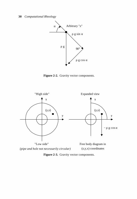
30 Computational Rheology
Arbitrary "z"
ρ g sin α
ρ g cos α
ρ g
α
90o
Figure 2-2. Gravity vector components.
x x
y y
(y,x) (y,x)
"High side" Expanded view
"Low side" Free body diagram in
(z,y,x) coordinates
− ρ g cos α
(pipe and hole not necessarily circular)
Figure 2-3. Gravity vector components.
Eccentric, Nonrotating, Annular Flow 31
If we introduce, without loss of generality, the pressure separation of variables
P = P(z,x) = p - zρg sin α + xρg cos α (2-26)
we can replace Equations 2-23, 2-24 and 2-25 by the single equation
∂Szy/∂y + ∂Szx/∂x = ∂P/∂z = constant (2-27)
where the constant pressure gradient ∂P/∂z is prescribed.Recall the definitions of the deformation tensor elements given in
Equations 2-6 to 2-11 and the fact that S = 2ND to rewrite Equation 2-27 as
∂ (N ∂u/∂y)/ ∂y + ∂ (N ∂u/∂x)/ ∂x = ∂P/∂z (2-28)
Here N(Γ) is, without approximation, given by the nonlinear equation
N(Γ) = k [ (∂u/∂y)2 + (∂u/∂x)2 ](n-1)/2 (2-29)
Equations 2-28 and 2-29 comprise the entire system to be solved along withgeneral no-slip velocity boundary conditions at drillpipe and borehole surfaces.
It is important, for the purposes of numerical analysis, to recognize howEquation 2-28 can be written as a nonlinear Poisson equation, that is,
∂2u/∂y2 + ∂2u/∂x2 = [∂P/∂z + (1-n)N(Γ)(uy2uyy
+2uyuxuyx +ux2uxx)/(uy
2 + ux2)] / N(Γ) (2-30)
In this form, conventional solution techniques for elliptic equations can beemployed. These include iterative techniques as well as direct inversionmethods. The nonlinear terms in the square brackets, for example, can beevaluated using latest values in a successive approximations scheme.
Also various algebraic simplifications are possible. For some values of n,particularly those near unity, these nonlinear terms may represent negligiblehigher order effects if the “1-n” terms are small in a dimensionless sensecompared with pressure gradient effects. For small n, the second derivativeterms on the right side may be unimportant since such flows contain flat velocityprofiles. Crochet, Davies and Walters (1984), which deals exclusively with non-Newtonian flows, presents discussions on different limit processes.
For the above limits, the principal effects of nonlinearity can be modeledusing the simpler and stabler Poisson model that results, one not unlike theclassical equation for Newtonian flow. Of course, the apparent viscosity thatacts in concert with the driving pressure gradient is still variable, nonlinear, anddependent on geometry and rate. For such cases only (and all solutions obtainedin this fashion should be checked a posteriori against the full equation) we have
∂2u/∂y2 + ∂2u/∂x2 ≈ N(Γ)-1 ∂P/∂z (2-31)
where Equation 2-29 is retained in its entirety. This approximation does notalways apply. But the strong influence of local geometry on annular velocity(e.g., low bottom speeds in eccentric holes regardless of rheology or flow rate)
32 Computational Rheology
suggests that any errors incurred by using Equation 2-31 may be insignificant.This simplification is akin to the “local linearization” used in nonlinearaerodynamics; in any case, the exact geometry of the annulus is always kept.
As noted earlier, borehole temperature may be important in drilling andproduction, but is probably not; thus, most studies neglect heat generation byinternal friction. Internal heat generation may affect local fluid viscosity since nand k depend on temperature. One way to estimate its importance is through thestrength of the temperature sources distributed within the annulus. The startingpoint is the energy equation for the temperature T(z,y,x,t). Even if velocity issteady in time, temperature does not have to be. For example, in a closedsystem, temperatures will increase if the borehole walls do not conduct heataway as quickly as it is produced; weak heat production can lead to largeincreases in T over time. Thus, whether or not frictional heat production issignificant, reduces to a matter of time scale and temperature boundaryconditions. If the increases are significant, the changes of viscosity as functionsof T must be modeled. This leads to mathematical complications; if the laminarviscosity µ = µ(T) in Newtonian flow depends on temperature, say, then themomentum and energy equations will couple through this dependence.
We will not consider this coupling yet. We assume that all rheologicalinput parameters are constants, so that our velocities obtain independently of T.Now the energy equation for T contains a positive definite quantity Φ called the“dissipation function” that is the distributed source term responsible for localheat generation. In general, it takes the form
Φ (z,y,x) = Szz∂u/∂z + Syy∂v/∂y + Sxx∂w/∂x
+ Szy(∂u/∂y + ∂v/∂z) + Szx(∂u/∂x + ∂w/∂z)
+ Syx(∂v/∂x + ∂w/∂y) (2-32)
Applying assumptions consistent with the foregoing analysis, we obtain
Φ = N(Γ) (∂u/∂y)2 + (∂u/∂x)2 > 0 (2-33)
where, as before, we use Equation 2-29 for the apparent viscosity in its entirety.Equation 2-33 shows that velocity gradients, not magnitudes, contribute totemperature increases.
In our computations, we provide values of local viscous stresses and theircorresponding shear rates. These stresses are the rectangular components
Szy = N(Γ) ∂u/∂y (2-34)
Szx = N(Γ) ∂u/∂x (2-35)
The shear rates corresponding to Equations 2-34 and 2-35 are ∂u/∂y and∂u/∂x respectively. These quantities are useful for several reasons. They arephysically important in estimating the efficiency with which fluids in deviatedwells remove cuttings beds having specified mechanical properties. From the
Eccentric, Nonrotating, Annular Flow 33
numerical analysis point of view, they allow checking of computed solutions forphysical consistency (e.g., high values at solid surfaces, zeros within plug flows)and required symmetries. We next discuss mathematical issues regardingcomputational grid generation and numerical solution. These ideas arehighlighted because we solve the complete boundary value problem, satisfyingno-slip velocity conditions exactly, without simplifying the annular geometry.
BOUNDARY CONFORMING GRID GENERATION
In many engineering problems, a judicious choice of coordinate systemssimplifies calculations and brings out the salient physical features moretransparently than otherwise. For example, the use of cylindrical coordinates forsingle well problems in petroleum engineering leads to elegant “radial flow”results that are useful in well testing. Cartesian grids, on the other hand, arepreferred in simulating oil and gas flows from rectangular fields.
The annular geometry modeling considered here is aimed at eccentricflows with cuttings beds, arbitrary borehole wall deformations, andunconventional drill collar or casing-centralizer cross-sections. Obviously,simple coordinate transforms are not readily available to handle arbitrarydomains of flow. Without resorting to crude techniques, for instance, applyingboundary conditions along mean circles and squares, or invoking “slot flow”assumptions, there has been no real reason for optimism until recently.
Fortunately, results from differential geometry allow us to construct“boundary conforming, natural coordinates” for computation. These generaltechniques extend classical ideas on conformal mapping. They have acceleratedprogress in simulating aerospace flows past airfoils and cascades, and are onlybeginning to be applied in the petroleum industry. Thompson, Warsi and Mastin(1985) provides an excellent introduction to the subject.
To those familiar with conventional analysis, it may seem that the choiceof (y,x) coordinates in Equation 2-31 is “unnatural.” After all, in the limit of aconcentric annulus, the equation does not reduce to a radial formulation. Butour use of such coordinates was motivated by the new gridding methods which,like classical conformal mapping, are founded on Cartesian coordinates. Theapproach in essence requires us to solve first a set of nonlinearly coupled,second-order PDEs. In particular, the equations
(yr2 + xr
2) yss - 2(ysyr + xs xr) ysr + (ys2 + xs
2) yrr = 0 (2-36)
(yr2 + xr
2) xss - 2(ysyr + xs xr) xsr + (ys2 + xs
2) xrr = 0 (2-37)
are considered with special mapping conditions related to the annular geometry.These are no simpler than the original flow equations, but they importantlyintroduce a first step that does not require solution on complicated domains.
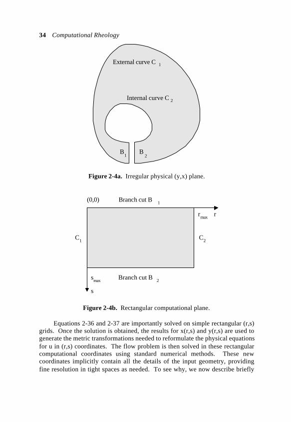
34 Computational Rheology
External curve C 1
Internal curve C 2
B1
B2
Figure 2-4a. Irregular physical (y,x) plane.
(0,0) Branch cut B 1
smax Branch cut B 2
C1 C2
rmax r
s
Figure 2-4b. Rectangular computational plane.
Equations 2-36 and 2-37 are importantly solved on simple rectangular (r,s)grids. Once the solution is obtained, the results for x(r,s) and y(r,s) are used togenerate the metric transformations needed to reformulate the physical equationsfor u in (r,s) coordinates. The flow problem is then solved in these rectangularcomputational coordinates using standard numerical methods. These newcoordinates implicitly contain all the details of the input geometry, providingfine resolution in tight spaces as needed. To see why, we now describe briefly
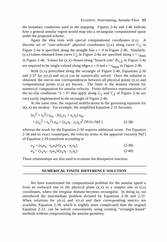
Eccentric, Nonrotating, Annular Flow 35
the boundary conditions used in the mapping. Figures 2-4a and 2-4b indicatehow a general annular region would map into a rectangular computational spaceunder the proposed scheme.
Again the idea rests with special computational coordinates (r,s). Adiscrete set of “user-selected” physical coordinates (y,x) along curve C1 in
Figure 2-4a is specified along the straight line r = 0 in Figure 2-4b. Similarly,(y,x) values obtained from curve C2 in Figure 2-4a are specified along r = rmaxin Figure 2-4b. Values for (y,x) chosen along “branch cuts” B1,2 in Figure 2-4a
are required to be single-valued along edges s = 0 and s = smax in Figure 2-4b.
With (y,x) prescribed along the rectangle of Figure 2-4b, Equations 2-36and 2-37 for y(r,s) and x(r,s) can be numerically solved. Once the solution isobtained, the one-to-one correspondences between all physical points (y,x) andcomputational points (r,s) are known. The latter is the domain chosen fornumerical computation for annular velocity. Finite difference representations ofthe no-slip conditions “u = 0” that apply along C1 and C2 of Figure 2-4a are
very easily implemented in the rectangle of Figure 2-4b.At the same time, the required modifications to the governing equation for
u(y,x) are modest. For example, the simplified Equation 2-31 becomes
(yr2 + xr
2) uss - 2(ysyr + xs xr) usr
+ (ys2 + xs
2) urr = (ys xr - yrxs )2 ∂P/∂z /N(Γ) (2-38)
whereas the result for the Equation 2-30 requires additional terms. For Equation2-38 and its exact counterpart, the velocity terms in the apparent viscosity N(Γ)of Equation 2-29 transform according to
uy = (xrus - xsur)/(ysxr - yrxs) (2-39)
ux = (ysur - yrus)/(ysxr - yrxs) (2-40)
These relationships are also used to evaluate the dissipation function.
NUMERICAL FINITE DIFFERENCE SOLUTION
We have transformed the computational problem for the annular speed ufrom an awkward one in the physical plane (y,x) to a simpler one in (r,s)coordinates, where the irregular domain becomes rectangular. In doing so, weintroduced the intermediate problem dictated by Equations 2-36 and 2-37.When solutions for y(r,s) and x(r,s) and their corresponding metrics areavailable, Equation 2-38, which is slightly more complicated than the originalEquation 2-31, can be solved conveniently using existing “rectangle-based”methods without compromising the annular geometry.
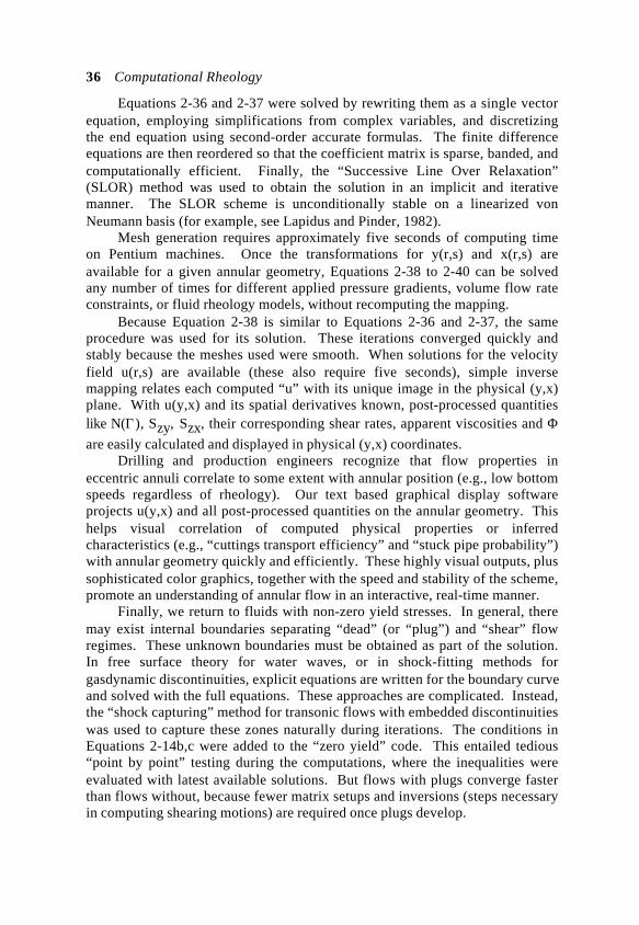
36 Computational Rheology
Equations 2-36 and 2-37 were solved by rewriting them as a single vectorequation, employing simplifications from complex variables, and discretizingthe end equation using second-order accurate formulas. The finite differenceequations are then reordered so that the coefficient matrix is sparse, banded, andcomputationally efficient. Finally, the “Successive Line Over Relaxation”(SLOR) method was used to obtain the solution in an implicit and iterativemanner. The SLOR scheme is unconditionally stable on a linearized vonNeumann basis (for example, see Lapidus and Pinder, 1982).
Mesh generation requires approximately five seconds of computing timeon Pentium machines. Once the transformations for y(r,s) and x(r,s) areavailable for a given annular geometry, Equations 2-38 to 2-40 can be solvedany number of times for different applied pressure gradients, volume flow rateconstraints, or fluid rheology models, without recomputing the mapping.
Because Equation 2-38 is similar to Equations 2-36 and 2-37, the sameprocedure was used for its solution. These iterations converged quickly andstably because the meshes used were smooth. When solutions for the velocityfield u(r,s) are available (these also require five seconds), simple inversemapping relates each computed “u” with its unique image in the physical (y,x)plane. With u(y,x) and its spatial derivatives known, post-processed quantitieslike N(Γ), Szy, Szx, their corresponding shear rates, apparent viscosities and Φare easily calculated and displayed in physical (y,x) coordinates.
Drilling and production engineers recognize that flow properties ineccentric annuli correlate to some extent with annular position (e.g., low bottomspeeds regardless of rheology). Our text based graphical display softwareprojects u(y,x) and all post-processed quantities on the annular geometry. Thishelps visual correlation of computed physical properties or inferredcharacteristics (e.g., “cuttings transport efficiency” and “stuck pipe probability”)with annular geometry quickly and efficiently. These highly visual outputs, plussophisticated color graphics, together with the speed and stability of the scheme,promote an understanding of annular flow in an interactive, real-time manner.
Finally, we return to fluids with non-zero yield stresses. In general, theremay exist internal boundaries separating “dead” (or “plug”) and “shear” flowregimes. These unknown boundaries must be obtained as part of the solution.In free surface theory for water waves, or in shock-fitting methods forgasdynamic discontinuities, explicit equations are written for the boundary curveand solved with the full equations. These approaches are complicated. Instead,the “shock capturing” method for transonic flows with embedded discontinuitieswas used to capture these zones naturally during iterations. The conditions inEquations 2-14b,c were added to the “zero yield” code. This entailed tedious“point by point” testing during the computations, where the inequalities wereevaluated with latest available solutions. But flows with plugs converge fasterthan flows without, because fewer matrix setups and inversions (steps necessaryin computing shearing motions) are required once plugs develop.
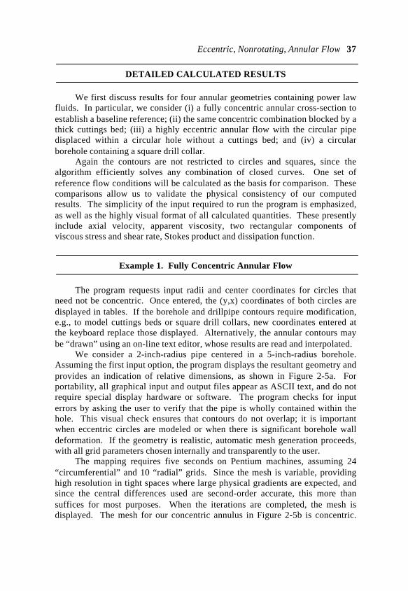
Eccentric, Nonrotating, Annular Flow 37
DETAILED CALCULATED RESULTS
We first discuss results for four annular geometries containing power lawfluids. In particular, we consider (i) a fully concentric annular cross-section toestablish a baseline reference; (ii) the same concentric combination blocked by athick cuttings bed; (iii) a highly eccentric annular flow with the circular pipedisplaced within a circular hole without a cuttings bed; and (iv) a circularborehole containing a square drill collar.
Again the contours are not restricted to circles and squares, since thealgorithm efficiently solves any combination of closed curves. One set ofreference flow conditions will be calculated as the basis for comparison. Thesecomparisons allow us to validate the physical consistency of our computedresults. The simplicity of the input required to run the program is emphasized,as well as the highly visual format of all calculated quantities. These presentlyinclude axial velocity, apparent viscosity, two rectangular components ofviscous stress and shear rate, Stokes product and dissipation function.
Example 1. Fully Concentric Annular Flow
The program requests input radii and center coordinates for circles thatneed not be concentric. Once entered, the (y,x) coordinates of both circles aredisplayed in tables. If the borehole and drillpipe contours require modification,e.g., to model cuttings beds or square drill collars, new coordinates entered atthe keyboard replace those displayed. Alternatively, the annular contours maybe “drawn” using an on-line text editor, whose results are read and interpolated.
We consider a 2-inch-radius pipe centered in a 5-inch-radius borehole.Assuming the first input option, the program displays the resultant geometry andprovides an indication of relative dimensions, as shown in Figure 2-5a. Forportability, all graphical input and output files appear as ASCII text, and do notrequire special display hardware or software. The program checks for inputerrors by asking the user to verify that the pipe is wholly contained within thehole. This visual check ensures that contours do not overlap; it is importantwhen eccentric circles are modeled or when there is significant borehole walldeformation. If the geometry is realistic, automatic mesh generation proceeds,with all grid parameters chosen internally and transparently to the user.
The mapping requires five seconds on Pentium machines, assuming 24“circumferential” and 10 “radial” grids. Since the mesh is variable, providinghigh resolution in tight spaces where large physical gradients are expected, andsince the central differences used are second-order accurate, this more thansuffices for most purposes. When the iterations are completed, the mesh isdisplayed. The mesh for our concentric annulus in Figure 2-5b is concentric.

38 Computational Rheology
Although our formulation for mesh generation problem was undertaken in (y,x)coordinates, it is clear that the end result must be the radial grid one anticipates.The power of the method is the extension of “radial” to complicated geometries.
X/Y orientation:
+---> Y | V X
11 11 11
11 11
11 11
11 11
1 1 1 1 1 11 1 1 11 1 1 1 1
11 1 1 11 1 1 1 1 11 1 1 11 1 1 1 1 1 11 11
11 11
11 11 11 11 11
Figure 2-5a. Concentric circular pipe and hole.
11 11 11 10 11 10 9 10 11 10 9 8 8 9 10 11 9 8 7 7 7 9 11 10 7 6 6 6 7 910 11 8 6 5 4 5 5 6 8 11 10 9 7 4 3 3 3 3 4 6 7 910 8 7 5 2 1 1 1 1 2 3 5 7 8 11 6 4 2 1 2 5 6 11 10 9 7 3 2 1 3 7 8 910 6 5 3 1 2 4 5 6
1110 9 8 7 6 4 3 1 2 4 5 6 8 910 11 3 1 2 3 8 7 6 5 1 1 4 5 7 8 11 10 9 5 4 2 1 1 3 5 91011 7 6 3 2 1 1 3 7 9 6 5 3 2 2 2 3 6 8 9 1110 7 5 4 4 3 4 5 7 1011 9 8 7 6 5 5 5 7 9 10 8 7 6 6 7 8 10 11 9 8 8 8 9 11 10 9 9 9 10 11 10 10 10 11 11 11 11
Figure 2-5b. Computed radial mesh system.
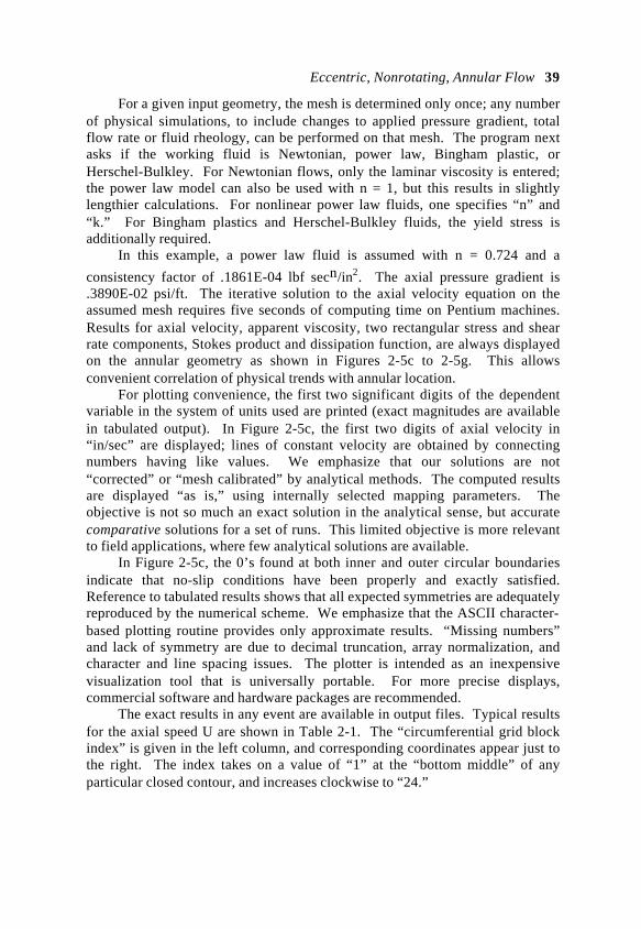
Eccentric, Nonrotating, Annular Flow 39
For a given input geometry, the mesh is determined only once; any numberof physical simulations, to include changes to applied pressure gradient, totalflow rate or fluid rheology, can be performed on that mesh. The program nextasks if the working fluid is Newtonian, power law, Bingham plastic, orHerschel-Bulkley. For Newtonian flows, only the laminar viscosity is entered;the power law model can also be used with n = 1, but this results in slightlylengthier calculations. For nonlinear power law fluids, one specifies “n” and“k.” For Bingham plastics and Herschel-Bulkley fluids, the yield stress isadditionally required.
In this example, a power law fluid is assumed with n = 0.724 and a
consistency factor of .1861E-04 lbf secn/in2. The axial pressure gradient is.3890E-02 psi/ft. The iterative solution to the axial velocity equation on theassumed mesh requires five seconds of computing time on Pentium machines.Results for axial velocity, apparent viscosity, two rectangular stress and shearrate components, Stokes product and dissipation function, are always displayedon the annular geometry as shown in Figures 2-5c to 2-5g. This allowsconvenient correlation of physical trends with annular location. For plotting convenience, the first two significant digits of the dependentvariable in the system of units used are printed (exact magnitudes are availablein tabulated output). In Figure 2-5c, the first two digits of axial velocity in“in/sec” are displayed; lines of constant velocity are obtained by connectingnumbers having like values. We emphasize that our solutions are not“corrected” or “mesh calibrated” by analytical methods. The computed resultsare displayed “as is,” using internally selected mapping parameters. Theobjective is not so much an exact solution in the analytical sense, but accuratecomparative solutions for a set of runs. This limited objective is more relevantto field applications, where few analytical solutions are available.
In Figure 2-5c, the 0’s found at both inner and outer circular boundariesindicate that no-slip conditions have been properly and exactly satisfied.Reference to tabulated results shows that all expected symmetries are adequatelyreproduced by the numerical scheme. We emphasize that the ASCII character-based plotting routine provides only approximate results. “Missing numbers”and lack of symmetry are due to decimal truncation, array normalization, andcharacter and line spacing issues. The plotter is intended as an inexpensivevisualization tool that is universally portable. For more precise displays,commercial software and hardware packages are recommended.
The exact results in any event are available in output files. Typical resultsfor the axial speed U are shown in Table 2-1. The “circumferential grid blockindex” is given in the left column, and corresponding coordinates appear just tothe right. The index takes on a value of “1” at the “bottom middle” of anyparticular closed contour, and increases clockwise to “24.”
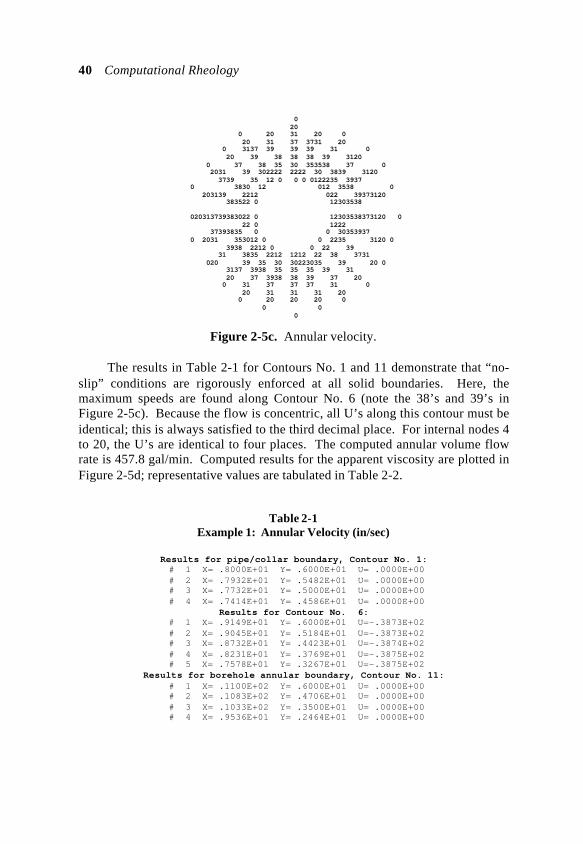
40 Computational Rheology
0 20 0 20 31 20 0 20 31 37 3731 20 0 3137 39 39 39 31 0 20 39 38 38 38 39 3120 0 37 38 35 30 353538 37 0 2031 39 302222 2222 30 3839 3120 3739 35 12 0 0 0 0122235 3937 0 3830 12 012 3538 0 203139 2212 022 39373120 383522 0 12303538
020313739383022 0 12303538373120 0 22 0 1222 37393835 0 0 30353937 0 2031 353012 0 0 2235 3120 0 3938 2212 0 0 22 39 31 3835 2212 1212 22 38 3731 020 39 35 30 30223035 39 20 0 3137 3938 35 35 35 39 31 20 37 3938 38 39 37 20 0 31 37 37 37 31 0 20 31 31 31 20 0 20 20 20 0 0 0 0
Figure 2-5c. Annular velocity.
The results in Table 2-1 for Contours No. 1 and 11 demonstrate that “no-slip” conditions are rigorously enforced at all solid boundaries. Here, themaximum speeds are found along Contour No. 6 (note the 38’s and 39’s inFigure 2-5c). Because the flow is concentric, all U’s along this contour must beidentical; this is always satisfied to the third decimal place. For internal nodes 4to 20, the U’s are identical to four places. The computed annular volume flowrate is 457.8 gal/min. Computed results for the apparent viscosity are plotted inFigure 2-5d; representative values are tabulated in Table 2-2.
Table 2-1Example 1: Annular Velocity (in/sec)
Results for pipe/collar boundary, Contour No. 1: # 1 X= .8000E+01 Y= .6000E+01 U= .0000E+00 # 2 X= .7932E+01 Y= .5482E+01 U= .0000E+00 # 3 X= .7732E+01 Y= .5000E+01 U= .0000E+00 # 4 X= .7414E+01 Y= .4586E+01 U= .0000E+00
Results for Contour No. 6: # 1 X= .9149E+01 Y= .6000E+01 U=-.3873E+02 # 2 X= .9045E+01 Y= .5184E+01 U=-.3873E+02 # 3 X= .8732E+01 Y= .4423E+01 U=-.3874E+02 # 4 X= .8231E+01 Y= .3769E+01 U=-.3875E+02 # 5 X= .7578E+01 Y= .3267E+01 U=-.3875E+02
Results for borehole annular boundary, Contour No. 11: # 1 X= .1100E+02 Y= .6000E+01 U= .0000E+00 # 2 X= .1083E+02 Y= .4706E+01 U= .0000E+00 # 3 X= .1033E+02 Y= .3500E+01 U= .0000E+00 # 4 X= .9536E+01 Y= .2464E+01 U= .0000E+00
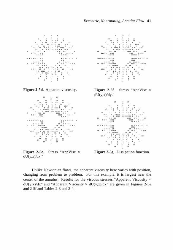
Eccentric, Nonrotating, Annular Flow 41
5 5 5 6 5 6 7 6 5 6 7 9 9 7 6 5 7 9 15 15 15 7 5 6 15 11 11 11 15 7 6 5 9 11 8 7 8 811 9 5 6 7 15 7 6 6 6 6 7 1115 7 6 915 8 6 5 5 5 5 6 6 8 15 9 5 11 7 6 5 6 811 5 6 715 6 6 5 6 15 9 7 6 11 8 6 5 6 7 811
5 6 7 91511 7 6 5 6 7 811 9 7 6 5 6 5 6 6 91511 8 5 5 7 815 9 5 6 7 8 7 6 5 5 6 8 7 6 5 1511 6 6 5 5 6 15 7 11 8 6 6 6 6 6 11 9 7 5 6 15 8 7 7 6 7 8 15 6 5
7 9 1511 8 8 8 15 7 6 9 1511 11 15 9 6 5 7 9 9 9 7 5 6 7 7 7 6 5 6 6 6 5 5 5 5
Figure 2-5d. Apparent viscosity.
29 30 29 25 26 24 17 24 26 22 17 10 917 22 21 15 8 2 2 2 15 21 18 2 6 6 6 2 1218 15 7 5 13 20 1311 5 7 15 12 8 2 172326 2726 17 4 2 812 5 1 9 2938 3938342919 9 1 5 7 310 24 2824 6 3 7 6 4 0 1317 1913 0 2 4 6 1 3 710 8 5 3 1
0 0 0 0 0 0 0 0 0 0 0 0 0 0 0 0 0 710 8 7 2 0 1 3 19 19 5 3 0 2 7 6 4 6101728 28 13 6 4 6 7
1 3 192434 34 19 1 8 4 9 2333 3633 23 4 5 8 1512 2 11 19 22261911 2 1215 12 7 2 5 13 14 13 2 12 18 8 2 6 7 2 8 18 21 15 9 10 9 15 21 22 17 18 17 22 26 24 27 24 26 29 29 32
Figure 2-5e. Stress “AppVisc ×dU(y,x)/dx.”
7 0 7 0 15 6 0 6 15 12 4 0 2 4 12 21 8 5 0 0 0 8 21 18 1 1 0 1 1 1218 26 7 3 3 0 3 6 3 7 26 2215 2 1013 7 0 7 10 4 2 1522 8 2 9 1710 010191719 9 2 8 29 517 24 2824 11 5 29 2417 2 2329 3423 2 91724 6132638 331913 6
30251710 2 6202739 342013 6101725 30 2638 3326 9 2 613 34 34 1913 2 9 29 2417 11172928 28 2311 172429 2 5 192419 19 19 2 15 4 9 13 8 0 8 13 4 815 2622 2 6 5 0 7 5 6 2 2226
12 7 1 3 3 0 3 1 12 18 5 0 1 0 0 5 18 21 8 2 0 2 8 21 12 4 0 4 12 15 6 0 6 15 7 7 0
Figure 2-5f. Stress “AppVisc ×dU(y,x)/dy.”
15 15 15 9 15 9 4 9 15 9 4 1 1 4 9 15 4 1 0 0 0 4 15 9 0 0 0 0 0 4 9 15 1 0 2 5 2 2 0 1 15 9 4 0 51111 1111 5 0 0 4 9 1 0 2 1928 2828281911 2 0 1
15 0 5 19 2819 2 0 15 9 4 0 1119 2811 0 1 4 9 0 21128 19 5 2 0
15 9 4 1 0 0 51128 19 5 2 0 1 4 9 15 1128 1911 1 0 0 2 28 28 5 2 0 1 15 9 4 2 51928 28 11 2 4 915 0 0 111928 28 11 0 4 0 2 1119 2219 11 0 1 4 15 9 0 2 5 611 5 2 0 915 4 1 0 0 2 2 2 0 4 9 1 0 0 0 0 1 9 15 4 1 1 1 4 15 9 4 4 4 9 15 9 11 9 15 15 15 18
Figure 2-5g. Dissipation function.
Unlike Newtonian flows, the apparent viscosity here varies with position,changing from problem to problem. For this example, it is largest near thecenter of the annulus. Results for the viscous stresses “Apparent Viscosity ×dU(y,x)/dx” and “Apparent Viscosity × dU(y,x)/dx” are given in Figures 2-5eand 2-5f and Tables 2-3 and 2-4.
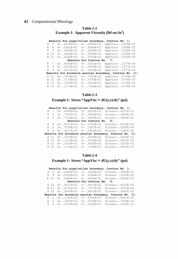
42 Computational Rheology
Table 2-2Example 1: Apparent Viscosity (lbf sec/in2)
Results for pipe/collar boundary, Contour No. 1: # 7 X= .6000E+01 Y= .4000E+01 AppVisc= .5558E-05 # 8 X= .5482E+01 Y= .4068E+01 AppVisc= .5558E-05 # 9 X= .5000E+01 Y= .4268E+01 AppVisc= .5558E-05 # 10 X= .4586E+01 Y= .4586E+01 AppVisc= .5558E-05 # 11 X= .4268E+01 Y= .5000E+01 AppVisc= .5558E-05
Results for Contour No. 7: # 7 X= .6000E+01 Y= .2541E+01 AppVisc= .1577E-04 # 8 X= .5105E+01 Y= .2659E+01 AppVisc= .1577E-04 # 9 X= .4271E+01 Y= .3005E+01 AppVisc= .1577E-04
Results for borehole annular boundary, Contour No. 11:# 11 X= .1670E+01 Y= .3500E+01 AppVisc= .5790E-05# 12 X= .1170E+01 Y= .4706E+01 AppVisc= .5790E-05# 13 X= .1000E+01 Y= .6000E+01 AppVisc= .5790E-05# 14 X= .1170E+01 Y= .7294E+01 AppVisc= .5790E-05
Table 2-3Example 1: Stress “AppVisc ×× dU(y,x)/dx” (psi)
Results for pipe/collar boundary, Contour No. 1: # 1 X= .8000E+01 Y= .6000E+01 Stress=-.4267E-03 # 2 X= .7932E+01 Y= .5482E+01 Stress=-.3864E-03 # 3 X= .7732E+01 Y= .5000E+01 Stress=-.3460E-03
Results for Contour No. 6: # 4 X= .8231E+01 Y= .3769E+01 Stress=-.4616E-04 # 5 X= .7578E+01 Y= .3267E+01 Stress=-.3260E-04 # 6 X= .6817E+01 Y= .2952E+01 Stress=-.1686E-04
Results for borehole annular boundary, Contour No. 11: # 11 X= .1670E+01 Y= .3500E+01 Stress=-.2660E-03 # 12 X= .1170E+01 Y= .4706E+01 Stress=-.2967E-03 # 13 X= .1000E+01 Y= .6000E+01 Stress=-.3072E-03 # 14 X= .1170E+01 Y= .7294E+01 Stress=-.2967E-03
Table 2-4Example 1: Stress “AppVisc ×× dU(y,x)/dy” (psi)
Results for pipe/collar boundary, Contour No. 1: # 8 X= .5482E+01 Y= .4068E+01 Stress= .3858E-03 # 9 X= .5000E+01 Y= .4268E+01 Stress= .3459E-03 # 10 X= .4586E+01 Y= .4586E+01 Stress= .2824E-03
Results for Contour No. 6: # 22 X= .8231E+01 Y= .8231E+01 Stress=-.4622E-04 # 23 X= .8732E+01 Y= .7577E+01 Stress=-.3270E-04 # 24 X= .9045E+01 Y= .6816E+01 Stress=-.1681E-04
Results for borehole annular boundary, Contour No. 11: # 1 X= .1100E+02 Y= .6000E+01 Stress=-.5091E-05 # 2 X= .1083E+02 Y= .4706E+01 Stress=-.7929E-04 # 3 X= .1033E+02 Y= .3500E+01 Stress=-.1535E-03

Eccentric, Nonrotating, Annular Flow 43
Table 2-5Example 1: Dissipation Function (lbf/(sec ×× sq in))
Results for pipe/collar boundary, Contour No. 1: # 6 X= .6518E+01 Y= .4068E+01 DissipFn= .2870E-01 # 7 X= .6000E+01 Y= .4000E+01 DissipFn= .2870E-01 # 8 X= .5482E+01 Y= .4068E+01 DissipFn= .2870E-01
Results for Contour No. 7: # 9 X= .4271E+01 Y= .3005E+01 DissipFn= .5235E-04 # 10 X= .3554E+01 Y= .3554E+01 DissipFn= .5236E-04 # 11 X= .3005E+01 Y= .4271E+01 DissipFn= .5236E-04 # 12 X= .2659E+01 Y= .5105E+01 DissipFn= .5237E-04 Results for borehole annular boundary, Contour No. 11: # 12 X= .1170E+01 Y= .4706E+01 DissipFn= .1629E-01 # 13 X= .1000E+01 Y= .6000E+01 DissipFn= .1629E-01 # 14 X= .1170E+01 Y= .7294E+01 DissipFn= .1629E-01 # 15 X= .1670E+01 Y= .8500E+01 DissipFn= .1629E-01
The plotting routine omits the signs of these stresses for visual clarity;signs and exact magnitudes are available from tabulated results. This test caseassuming concentric flow is important for numerical validation. The dU(y,x)/dxstress is symmetric with respect to the horizontal center line, as required, andvanishes there; similarly, the dU(y,x)/dy stress is symmetric with respect to thevertical center line and is zero there. These physically correct results appear asthe result of properly converged iterations. Finally, results for the dissipationfunction are shown in Figure 2-5g and Table 2-5. Note how the greatest heatgeneration occurs at the pipe surface and at the borehole wall; there is minimaldissipation at the midpoint of the annulus.
Example 2. Concentric Pipe and Boreholein the Presence of a Cuttings Bed
For comparison, consider the same annular geometry used before, that is, a2-inch-radius pipe located within a concentric 5-inch-radius borehole. But whenthe program requests modifications to the outer contour, we overwrite five of thebottom coordinates to simulate a flat cuttings bed. The bed height is half of thedistance up the annular cross-section. This blockage should reduce the “457.8gal/min” obtained in Example 1 for the unblocked annulus. First, the programgenerates the grid in Figure 2-6a, which conforms to the top of the cuttings bed.For comparison with Example 1, we again assume n = 0.7240 and a “k” of
.1861E-04 lbf secn/in2. The pressure gradient is the same .3890E-02 psi/ft.Figure 2-6b shows that the maximum velocities at the bottom are less than one-half of those at the top. This trend is well known qualitatively, but the programallows us to obtain exact velocities everywhere without making unrealistic “slotflow” assumptions. The low velocities adjacent to the bed imply that cuttingstransport will not be very efficient just above it, and that stuck pipe is possible.
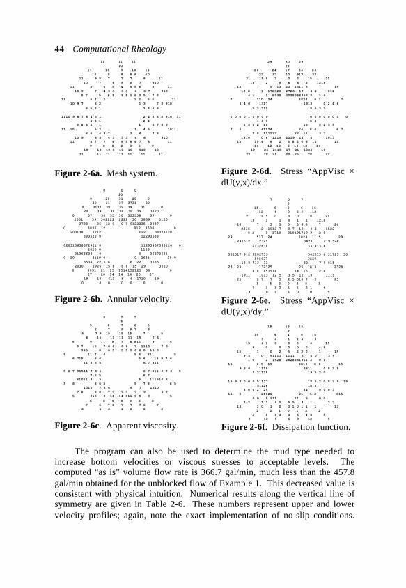
44 Computational Rheology 11 11 11 10 11 10 9 10 11 10 9 8 8 9 10 11 9 8 7 7 7 9 11 10 7 6 6 6 7 910 11 8 6 5 4 5 5 6 8 11 10 9 7 4 3 3 3 3 4 6 7 910 8 7 5 2 1 1 1 1 2 3 5 7 8 11 6 4 2 1 2 5 6 11 10 9 7 3 2 1 3 7 8 910
6 5 3 1 2 4 5 6
1110 9 8 7 6 4 3 1 2 4 5 6 8 910 11 4 3 1 2 4 9 8 6 5 1 1 6 7 8 9 11 10 5 3 1 1 4 5 1011 8 6 4 3 2 2 4 7 8 10 9 6 5 4 3 3 3 4 6 910 11 8 7 7 6 6 5 6 6 7 8 11 9 8 8 8 8 8 9 10 10 10 9 10 10 910 10 11 11 11 11 11 11 11
Figure 2-6a. Mesh system.
0 0 0 20 0 20 31 20 0 20 31 37 3731 20 0 3137 39 39 39 31 0 20 39 38 38 38 39 3120 0 37 38 35 30 353538 37 0 2031 39 302222 2222 30 3839 3120 3738 35 12 0 0 0 0122235 3837 0 3830 12 012 3538 0 203138 2212 022 38373120 383522 0 12293538
020313638372921 0 11293437363120 0 2820 0 1128 31363633 0 0 36373631 0 20 3119 0 0 2631 20 0 3534 2215 6 6 22 3535 2030 2926 15 8 8 8 15 29 3020 0 3031 21 15 1514152121 30 0 27 20 14 14 14 20 27 19 10 611 6 6 1710 19 0 0 0 0 0 0 0
Figure 2-6b. Annular velocity.
5 5 5 6 5 6 7 6 5 6 7 9 9 7 6 5 7 9 15 15 15 7 5 6 15 11 11 11 15 7 6 5 9 11 8 7 8 811 9 5 6 7 15 7 6 6 6 6 7 1115 7 6 915 8 6 5 5 5 5 6 6 8 15 9 5 11 7 6 5 6 811 5 6 715 6 6 5 6 15 9 7 6 11 8 6 5 6 7 811
5 6 7 91511 7 6 5 6 7 811 9 7 6 5 7 6 5 6 7 81011 8 5 5 111510 8 5 6 8 6 5 5 7 8 6 5 1010 7 6 6 6 7 1310 7 8 9 8 7 7 7 7 7 9 8 7 5 910 9 11 14 911 9 9 9 5
8 8 9 9 9 8 8 7 6 7 8 7 7 7 6 7 6 6 6 6 6 6 6
Figure 2-6c. Apparent viscosity.
29 30 29 25 26 24 17 24 26 22 17 10 917 22 21 15 8 2 2 2 15 21 18 2 6 6 6 2 1218 15 7 5 13 20 1311 5 7 15 12 8 1 172326 2726 17 4 1 812 4 1 9 2938 3938342919 9 1 4 7 310 24 2824 6 3 7 6 4 0 1317 1913 0 2 4 6
2 3 710 8 5 3 2
0 0 0 0 1 0 0 0 0 0 0 0 0 0 0 0 0 4 6 9 8 4 5 3 0 2 18 18 0 2 3 5 7 6 41124 24 8 4 6 7 7 0 111522 22 11 3 7 1310 0 6 1219 2019 12 0 1013 15 10 4 6 2 5 8 2 0 6 10 15 14 12 10 8 10 12 14 19 24 2115 17 21 1824 19 22 28 25 20 25 28 22
Figure 2-6d. Stress “AppVisc ×dU(y,x)/dx.”
7 0 7 0 15 6 0 6 15 12 4 0 2 4 12 21 8 5 0 0 0 8 21 18 1 1 0 1 1 1218 26 7 3 3 0 3 6 3 7 26 2215 2 1013 7 0 7 10 4 2 1522 8 2 9 1710 010191719 9 2 8 29 517 24 2824 11 5 29 2415 2 2329 3423 2 91524
6132638 331913 6
302517 9 2 6202739 342013 6 91725 30 202637 3220 15 8 713 32 32 7 0 815 28 23 132325 25 1813 2328 4 8 151914 14 15 2 4 1911 1013 12 5 3 5 12 10 1119 23 2 7 7 5 2 5 510 7 2 23 1 5 3 0 3 5 1 6 1 1 2 1 1 2 1 6 9 0 0 1 0 0 9
Figure 2-6e. Stress “AppVisc ×dU(y,x)/dy.”
15 15 15 9 15 9 4 9 15 9 4 1 1 4 9 15 4 1 0 0 0 4 15 9 0 0 0 0 0 4 9 15 1 0 2 5 2 2 0 1 15 9 3 0 51111 1111 5 0 0 3 9 1 0 2 1928 2828281911 2 0 1 15 0 5 19 2819 2 0 15 9 3 0 1119 2811 0 0 3 9 0 21128 19 5 2 0
15 9 3 0 0 0 51127 18 5 2 0 0 3 9 15 51126 18 5 3 0 0 2 24 24 0 0 0 3 15 8 21021 21 5 2 815 0 0 5 911 11 5 0 0 7 2 1 2 4 5 5 5 4 1 2 7 13 1 0 1 0 0 1 0 1 1 1 13 2 2 1 0 1 2 2 5 8 6 3 4 6 4 8 5 9 13 9 6 9 13 9
Figure 2-6f. Dissipation function.
The program can also be used to determine the mud type needed toincrease bottom velocities or viscous stresses to acceptable levels. Thecomputed “as is” volume flow rate is 366.7 gal/min, much less than the 457.8gal/min obtained for the unblocked flow of Example 1. This decreased value isconsistent with physical intuition. Numerical results along the vertical line ofsymmetry are given in Table 2-6. These numbers represent upper and lowervelocity profiles; again, note the exact implementation of no-slip conditions.
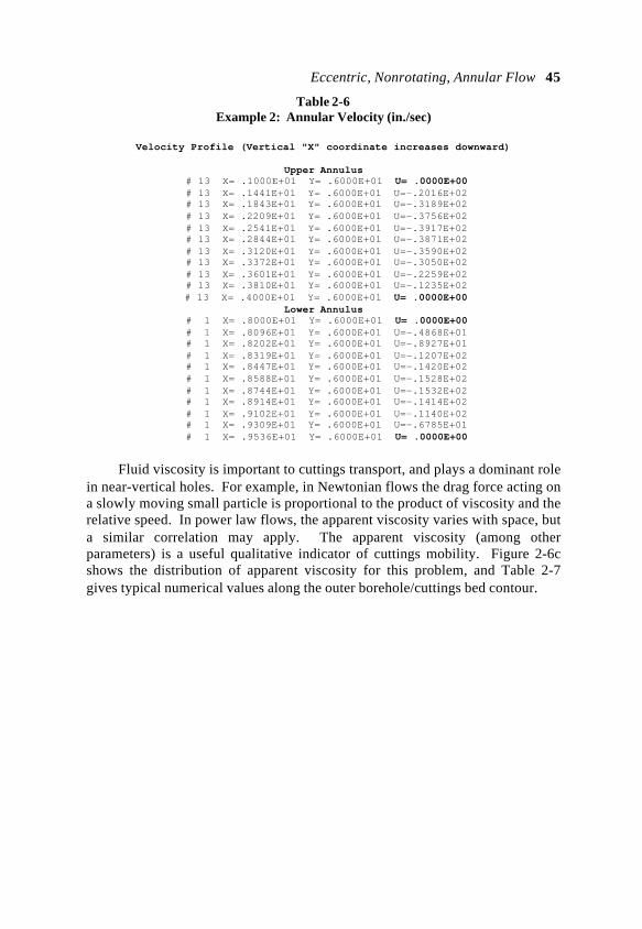
Eccentric, Nonrotating, Annular Flow 45
Table 2-6Example 2: Annular Velocity (in./sec)
Velocity Profile (Vertical "X" coordinate increases downward)
Upper Annulus # 13 X= .1000E+01 Y= .6000E+01 U= .0000E+00 # 13 X= .1441E+01 Y= .6000E+01 U=-.2016E+02 # 13 X= .1843E+01 Y= .6000E+01 U=-.3189E+02 # 13 X= .2209E+01 Y= .6000E+01 U=-.3756E+02 # 13 X= .2541E+01 Y= .6000E+01 U=-.3917E+02 # 13 X= .2844E+01 Y= .6000E+01 U=-.3871E+02 # 13 X= .3120E+01 Y= .6000E+01 U=-.3590E+02 # 13 X= .3372E+01 Y= .6000E+01 U=-.3050E+02 # 13 X= .3601E+01 Y= .6000E+01 U=-.2259E+02 # 13 X= .3810E+01 Y= .6000E+01 U=-.1235E+02 # 13 X= .4000E+01 Y= .6000E+01 U= .0000E+00
Lower Annulus # 1 X= .8000E+01 Y= .6000E+01 U= .0000E+00 # 1 X= .8096E+01 Y= .6000E+01 U=-.4868E+01 # 1 X= .8202E+01 Y= .6000E+01 U=-.8927E+01 # 1 X= .8319E+01 Y= .6000E+01 U=-.1207E+02 # 1 X= .8447E+01 Y= .6000E+01 U=-.1420E+02 # 1 X= .8588E+01 Y= .6000E+01 U=-.1528E+02 # 1 X= .8744E+01 Y= .6000E+01 U=-.1532E+02 # 1 X= .8914E+01 Y= .6000E+01 U=-.1414E+02 # 1 X= .9102E+01 Y= .6000E+01 U=-.1140E+02 # 1 X= .9309E+01 Y= .6000E+01 U=-.6785E+01 # 1 X= .9536E+01 Y= .6000E+01 U= .0000E+00
Fluid viscosity is important to cuttings transport, and plays a dominant rolein near-vertical holes. For example, in Newtonian flows the drag force acting ona slowly moving small particle is proportional to the product of viscosity and therelative speed. In power law flows, the apparent viscosity varies with space, buta similar correlation may apply. The apparent viscosity (among otherparameters) is a useful qualitative indicator of cuttings mobility. Figure 2-6cshows the distribution of apparent viscosity for this problem, and Table 2-7gives typical numerical values along the outer borehole/cuttings bed contour.

46 Computational Rheology
Table 2-7Example 2: Apparent Viscosity (lbf sec/in.2)
Results for borehole annular boundary, Contour No. 11: # 1 X= .9536E+01 Y= .6000E+01 AppVisc= .6895E-05 # 2 X= .9536E+01 Y= .5000E+01 AppVisc= .6545E-05 # 3 X= .9536E+01 Y= .4000E+01 AppVisc= .6196E-05 # 4 X= .9535E+01 Y= .2464E+01 AppVisc= .6421E-05
.
. # 19 X= .6000E+01 Y= .1100E+02 AppVisc= .5789E-05 # 20 X= .7294E+01 Y= .1083E+02 AppVisc= .5793E-05 # 21 X= .8500E+01 Y= .1033E+02 AppVisc= .5875E-05 # 22 X= .9535E+01 Y= .9535E+01 AppVisc= .6421E-05 # 23 X= .9536E+01 Y= .8000E+01 AppVisc= .6196E-05 # 24 X= .9536E+01 Y= .7000E+01 AppVisc= .6545E-05
Axial velocity and apparent viscosity play direct roles in the dynamics ofindividual cuttings in near-vertical holes. The stability of the beds formed byparticles that have descended to the lower side of the annulus in horizontal orhighly deviated holes is also of interest. In this respect, the viscous fluid shearstresses acting at the surface of the cuttings bed are important. If they exceedthe bed yield stress, then it is likely that the bed will erode. The program can beused to determine which powers and consistency factors are needed to erodebeds with known mechanical yield properties. There are two relevantcomponents of viscous fluid stress, namely, “Apparent Viscosity × dU(y,x)/dx”and “Apparent Viscosity × dU(y,x)/dy.”
Table 2-8
Example 2: Stress “AppVisc ×× dU(y,x)/dx” (psi)
Results for borehole annular boundary, Contour No. 11: # 1 X= .9536E+01 Y= .6000E+01 Stress= .2068E-03 # 2 X= .9536E+01 Y= .5000E+01 Stress= .2508E-03 # 3 X= .9536E+01 Y= .4000E+01 Stress= .2888E-03 # 4 X= .9535E+01 Y= .2464E+01 Stress= .2289E-03 # 5 X= .8500E+01 Y= .1670E+01 Stress= .1501E-03 # 6 X= .7294E+01 Y= .1170E+01 Stress= .7748E-04 # 7 X= .6000E+01 Y= .1000E+01 Stress= .1265E-06 # 8 X= .4706E+01 Y= .1170E+01 Stress=-.7871E-04
.
. # 14 X= .1170E+01 Y= .7294E+01 Stress=-.2964E-03 # 15 X= .1670E+01 Y= .8500E+01 Stress=-.2656E-03 # 16 X= .2464E+01 Y= .9535E+01 Stress=-.2166E-03 # 17 X= .3500E+01 Y= .1033E+02 Stress=-.1528E-03 # 18 X= .4706E+01 Y= .1083E+02 Stress=-.7871E-04 # 19 X= .6000E+01 Y= .1100E+02 Stress= .1265E-06 # 20 X= .7294E+01 Y= .1083E+02 Stress= .7748E-04 # 21 X= .8500E+01 Y= .1033E+02 Stress= .1501E-03 # 22 X= .9535E+01 Y= .9535E+01 Stress= .2289E-03 # 23 X= .9536E+01 Y= .8000E+01 Stress= .2888E-03 # 24 X= .9536E+01 Y= .7000E+01 Stress= .2507E-03

Eccentric, Nonrotating, Annular Flow 47
Computed results for the absolute value of viscous stress are plotted inFigures 2-6d and 2-6e; actual stresses along the borehole/cuttings bed contourare explicitly given in Tables 2-8 and 2-9. In Figure 2-6d, the weak symmetryabout the horizontal row of zeros indicates that the influence of the bed is a localone (the “zeros” actually contain unprinted fractional values). But although bedeffects are local in this sense, they do affect total flow rate significantly, as isknown experimentally and computed here.
Table 2-9
Example 2: Stress “AppVisc ×× dU(y,x)/dy” (psi)
Results for borehole annular boundary, Contour No. 11: # 1 X= .9536E+01 Y= .6000E+01 Stress= .1115E-04 # 2 X= .9536E+01 Y= .5000E+01 Stress= .3537E-05 # 3 X= .9536E+01 Y= .4000E+01 Stress=-.3319E-05 # 4 X= .9535E+01 Y= .2464E+01 Stress=-.9696E-04 # 5 X= .8500E+01 Y= .1670E+01 Stress=-.2353E-03 # 6 X= .7294E+01 Y= .1170E+01 Stress=-.2845E-03 # 7 X= .6000E+01 Y= .1000E+01 Stress=-.3012E-03
.
. # 15 X= .1670E+01 Y= .8500E+01 Stress= .1533E-03 # 16 X= .2464E+01 Y= .9535E+01 Stress= .2166E-03 # 17 X= .3500E+01 Y= .1033E+02 Stress= .2646E-03 # 18 X= .4706E+01 Y= .1083E+02 Stress= .2937E-03 # 19 X= .6000E+01 Y= .1100E+02 Stress= .3012E-03 # 20 X= .7294E+01 Y= .1083E+02 Stress= .2845E-03 # 21 X= .8500E+01 Y= .1033E+02 Stress= .2353E-03 # 22 X= .9535E+01 Y= .9535E+01 Stress= .9696E-04 # 23 X= .9536E+01 Y= .8000E+01 Stress= .3319E-05 # 24 X= .9536E+01 Y= .7000E+01 Stress=-.3537E-05
Finally, Figure 2-6f displays the dissipation function as it varies in theannular cross-section. In this example, the lower part of the annulus near thecuttings bed is relatively nondissipative. Typical results are given in Table 2-10.
Table 2-10Example 2: Dissipation Function (lbf/(sec ×× in.2))
Results for pipe/collar boundary, Contour No. 1: # 1 X= .8000E+01 Y= .6000E+01 DissipFn= .1157E-01 # 2 X= .7932E+01 Y= .5482E+01 DissipFn= .1249E-01 # 3 X= .7732E+01 Y= .5000E+01 DissipFn= .1597E-01 # 4 X= .7414E+01 Y= .4586E+01 DissipFn= .2124E-01 # 5 X= .7000E+01 Y= .4268E+01 DissipFn= .2488E-01
.
. # 18 X= .5482E+01 Y= .7932E+01 DissipFn= .2813E-01 # 19 X= .6000E+01 Y= .8000E+01 DissipFn= .2766E-01 # 20 X= .6518E+01 Y= .7932E+01 DissipFn= .2675E-01 # 21 X= .7000E+01 Y= .7732E+01 DissipFn= .2488E-01 # 22 X= .7414E+01 Y= .7414E+01 DissipFn= .2124E-01 # 23 X= .7732E+01 Y= .7000E+01 DissipFn= .1597E-01 # 24 X= .7932E+01 Y= .6518E+01 DissipFn= .1249E-01
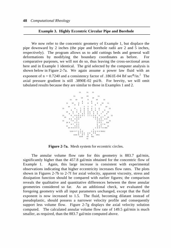
48 Computational Rheology
Example 3. Highly Eccentric Circular Pipe and Borehole
We now refer to the concentric geometry of Example 1, but displace thepipe downward by 2 inches (the pipe and borehole radii are 2 and 5 inches,respectively). The program allows us to add cuttings beds and general walldeformations by modifying the boundary coordinates as before. Forcomparative purposes, we will not do so, thus leaving the cross-sectional areashere and in Example 1 identical. The grid selected by the computer analysis isshown below in Figure 2-7a. We again assume a power law fluid with an
exponent of n = 0.7240 and a consistency factor of .1861E-04 lbf secn/in.2 Theaxial pressure gradient is still .3890E-02 psi/ft. For brevity, we will omittabulated results because they are similar to those in Examples 1 and 2.
11 11 11
11 10 11 10 10 11 10 9 10 11 9 9 11 10 9 8 8 8 9 10 11 9 8 8 9 10 7 7 7 10 11 8 7 6 6 6 7 8 11 9 7 6 5 5 5 6 7 9 10 8 6 5 4 4 4 5 6 8 10 9 7 5 4 3 2 3 4 5 7 9 11 8 6 5 4 3 2 1 1 1 1 2 4 6 8 11 10 7 4 3 2 1 2 4 6 7 10 9 8 5 4 2 1 2 4 5 8 9 11 7 6 3 2 3 6 7 11 10 9 5 3 1 1 4 5 910 8 7 2 1 2 6 7 8 11 5 4 1 2 4 5 11 10 9 8 6 5 3 1 4 6 7 8 910 1 1 1110 9 7 5 3 2 1 2 4 6 8 91011 8 7 4 4 4 4 5 8 1110 9 8 7 8 8 1011 1110 10 911
11
Figure 2-7a. Mesh system for eccentric circles.
The annular volume flow rate for this geometry is 883.7 gal/min,significantly higher than the 457.8 gal/min obtained for the concentric flow ofExample 1. Again, this large increase is consistent with experimentalobservations indicating that higher eccentricity increases flow rates. The plotsshown in Figures 2-7b to 2-7f for axial velocity, apparent viscosity, stress anddissipation function should be compared with earlier figures; the comparisonreveals the qualitative and quantitative differences between the three annulargeometries considered so far. As an additional check, we evaluated theforegoing geometry with all input parameters unchanged, except that the fluidexponent is now increased to 1.5. The fluid, becoming dilatant instead ofpseudoplastic, should possess a narrower velocity profile and consequentlysupport less volume flow. Figure 2-7g displays the axial velocity solutioncomputed. The calculated annular volume flow rate of 149.5 gal/min is muchsmaller, as required, than the 883.7 gal/min computed above.
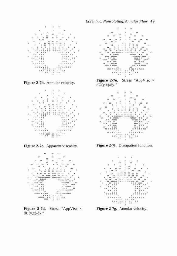
Eccentric, Nonrotating, Annular Flow 49 0 0 0
0 7 0 7 7 0 6 10 6 0 10 10 0 6 9 11 11 11 9 6 0 8 10 10 8 5 11 11 11 5 0 9 10 10 11 10 10 9 0 7 9 10 9 9 9 10 9 7
4 8 9 9 7 8 7 9 9 8 4 6 8 8 7 5 3 5 7 8 8 6 0 7 7 6 6 4 2 0 0 0 0 2 6 7 7 0 3 6 5 3 2 0 2 5 6 6 3 4 5 5 4 2 0 2 4 5 5 4 0 5 4 3 1 3 4 5 0 2 3 4 2 0 0 3 4 3 2 3 3 1 0 1 3 3 3 0 2 2 0 0 2 2 0 1 2 2 2 1 0 0 1 2 2 2 2 1 0 0 0 0 1 1 1 0 0 0 0 0 1 1 1 0 0 0 0 0 0 0 0 0 0 0 0 0 0 0 0 0 0 0 0 0 0 0 0 0
Figure 2-7b. Annular velocity.
4 4 4
4 6 4 6 6 4 6 7 6 4 7 7 5 5 7 9 10 9 7 5 5 6 9 9 6 5 11 12 11 5
5 8 10 8 8 8 10 8 5 6 9 8 6 6 6 8 9 6 6 7 7 6 6 5 6 6 7 7 6 6 8 6 6 5 5 5 6 6 8 6 5 7 7 6 6 5 5 4 4 4 4 5 6 7 7 5 6 8 6 5 5 4 5 6 7 8 6 6 7 7 6 5 5 5 6 7 7 6 5 8 7 5 5 5 7 8 5 6 6 7 6 5 5 6 7 6 6 7 8 5 5 5 8 8 7 5 7 7 6 6 7 7 5 6 7 8 8 8 7 6 7 8 8 8 7 6 7 7 6 7 7 9 9 8 8 7 8 810 8 7 7 6 911 910 1110 10 9 7 7 8 1114 13 11 7 7 7 9 10 10 7 8
Figure 2-7c. Apparent viscosity.
41 42 41
37 35 37 34 34 30 30 21 30 30 20 20
20 23 17 8 9 8 17 23 20 11 5 5 11 14 6 5 6 14 9 1 7 15 15 15 7 1 9 4 9 17 26 26 26 17 9 4 4 4 17 25 35 3635 25 17 4 4 2 12 24 3345 5745 33 24 12 2 1 9 182129344862 6562544829 18 9 1 5 14 242639 423924 1714 5 913 181827 28271818 13 9 11 1515 17 15171515 11 1214 14 813 131114 1412 1515 4 0 4 121515 18 8 4 8 4 4 8 18 171515 8 4 5 13 0 812151517 15 15 201815 9 0 812 1412 4 412151820 9 6 6 7 8 7 2 9 181512 6 3 1 6 1518 1412 6 914 8
Figure 2-7d. Stress “AppVisc ×dU(y,x)/dx.”
11 0 11
22 0 22 10 10 31 20 0 20 31 7 7 38 28 15 5 0 5 15 28 38 21 11 11 21 33 3 0 3 33 41 14 5 0 0 0 5 14 41
24 7 0 3 0 3 0 7 24 35 15 1 6 6 0 6 6 1 15 35 25 7 9 12 9 0 9 12 9 7 25 41 15 31217252515 015302517 3 15 41 34 5 213034 413421 4 5 34 2314 142339 46392314 1423 36 3 7 32 3932 7 3 36 2919 153046 462315 1929 10 0 3641 36 8 010 28 152133 302115 28 2213 5 81320 2417 8 1 51322 15 15 1813 7 31013 8 8 812 7 1 71318 0 3 7 3 2 3 7 0 9 6 3 0 1 0 0 6 9 3 2 3 0 3 4
Figure 2-7e. Stress “AppVisc ×dU(y,x)/dy.”
38 38 38
38 21 38 21 21 38 21 6 21 38 6 6 37 22 7 1 0 1 7 22 37 8 1 1 8
22 0 0 0 22 35 2 0 3 3 3 0 2 35 9 1 3 10 10 10 3 1 9 21 3 4 10 21 2221 10 4 3 21 9 2 9 2139 6439 21 9 2 9 31 4 4 919335889 9189825819 4 4 31 19 3 172851 725117 4 3 19 9 4 71342 594213 7 4 9 26 3 3 22 3222 3 3 26 15 8 61544 4410 6 815 4 2 2231 22 2 2 4 19 4 619 14 6 4 19 12 6 3 1 2 5 11 3 1 1 3 612 6 6 11 7 3 1 1 3 2 3 2 2 0 1 3 711 0 0 0 0 0 0 0 0 6 3 1 0 0 0 0 3 6 2 1 0 0 2 1
Figure 2-7f. Dissipation function.
0 0 0
0 10 0 10 10
0 9 17 9 0 17 17 0 8 15 20 21 20 15 8 0 14 19 19 14 7 21 22 21 7 0 17 19 19 20 19 19 17 0 12 17 18 15 17 15 18 17 12 6 14 15 15 12 1312 15 15 14 6 10 14 13 11 8 4 8 11 13 14 10 0 11 131110 7 4 0 0 0 0 410 13 11 0 4 12 8 6 3 0 3 8 1112 4 7 9 9 7 3 0 3 7 9 9 7 0 9 8 4 2 4 8 9 0 3 5 7 3 0 0 5 7 5 3 6 6 1 0 1 6 6 6 0 5 4 0 1 4 5 0 2 3 4 4 3 2 0 3 4 4 4 3 2 0 0 0 1 2 3 2 1 0 0 0 2 3 3 2 1 0 2 2 1 1 1 1 2 2 0 1 1 1 1 1 1 1 0 0 0 0 1 0 0
Figure 2-7g. Annular velocity.

50 Computational Rheology
Example 4. Square Drill Collar in a Circular Hole
Square drill collars are sometimes used to control drillpipe sticking anddogleg severity. In this final comparative example, we consider a 5-inch-radiusborehole containing a centered square drill collar having 4-inch sides. Theserelative dimensions are selected for plotting purposes only. In all cases, thefinite difference program will accurately calculate and tabulate output quantities,even if the ASCII plotter lacks sufficient spatial resolution.
We will assume the same flow parameters as Example 1, where we hadobtained peak annular velocities of 39 in./sec and a total flow rate of 457.8gal/min. But here, tabulated results show that peak velocities of 33 in./sec areobtained near the center of the annulus; also, the total volume flow rate is 334.7gal/min. The corresponding velocity plot is shown in Figure 2-8a.
These rates are smaller than those of Example 1 because the “4-inchsquare” blocks more area than its inscribed “4-inch-diameter circle.” Thus,computed results are consistent with behavior expected on physical grounds.Figures 2-8b to 2-8e are given without discussion; note how the outline of thesquare drill collar is adequately represented throughout.
0 0 0 15 15 15 0 25 26 25 0 14 30 31 30 2214 0 27 32 33 32 27 12 0 20 29 3230 31 32 2929 2420 0 26 27 26 27 26 27 2526 0 14 23 17 11 12 11 9171423 2214 2729 7 0 0 0 0 0 7 292927 0 2717 0 92327 0 1525303232 32302515 302611 0 112030
015263133312712 0 1221313333312615 0 0 0 3032322611 1120303230 01525 9 0 9 2515 0 292717 2329 222729 14 7 9 10 10 010 9 14 2922 014 2523 22 18 24 18 22 25 14 0 2425 2826 28 28 28 28 24 1220 28 30 30 30 28 12 0 2226 29 29 29 22 0 14 24 24 24 14 0 15 15 15 0 0 0 0
Figure 2-8a. Annular velocity, square drill collar.
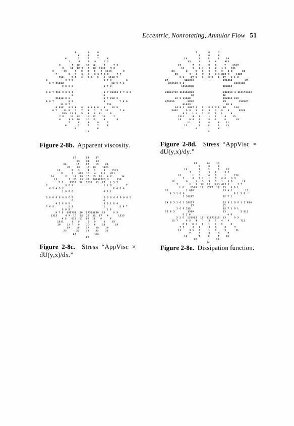
Eccentric, Nonrotating, Annular Flow 51
6 5 6 6 6 6 6 7 7 7 6 7 9 9 9 7 7
6 9 12 13 12 9 7 6 8 12 12 9 9 12 1112 9 8 6 15 9 8 8 8 9 1115 6 7 8 7 6 6 6 6 7 6 8 7 7 912 5 5 6 5 6 5 5 1112 9 6 9 7 5 6 7 9 6 6 7 91212 12 9 7 6 9 8 6 6 6 7 9
5 6 7 913 9 8 6 5 6 7 91313 9 7 6 5 6 6 91212 8 6 6 7 912 9 6 6 7 6 5 6 7 6 6 11 9 7 711 8 912 6 5 6 6 6 6 6 6 6 12 8 6 7 11 8 7 7 8 7 7 11 7 6 915 11 9 9 9 9 11 9 7 8 13 12 13 12 13 7 6 8 9 10 10 10 8 6 7 8 8 8 7 6 7 7 7 6 6 6 5
Figure 2-8b. Apparent viscosity.
27 29 27
23 24 23 24 15 17 15 24 20 10 10 10 1420 19 8 3 4 3 8 1519 11 1 410 10 4 6 1 611 14 2 12 15 15 15 12 4 2 14 12 9 23 28 28 28292320 9 912 7 5 2733 32 3232 33 27 1 5 7 7 0 2 1 1 1 0 7 6 5 4 3 2 2 4 5 6 1 0 0 0 0 0 1
0 0 0 0 0 0 0 0 0 0 0 0 0 0 0 0 0 0 0 0 4 3 2 0 0 0 0 1 2 4 7 6 5 1 1 1 5 6 7 2 0 2 1 2 9 7 5 202728 28 27322828 20 5 9 1312 4 9 17 22 15 22 17 4 1213 6 2 612 11 10 11 6 6 1511 1 5 3 5 1 15 19 13 7 8 10 8 13 19 19 15 17 15 19 23 22 25 22 23
26 26 29
Figure 2-8c. Stress “AppVisc ×dU(y,x)/dx.”
7 0 7 6 0 6 14 5 0 5 14 12 4 0 4 912
19 7 3 0 3 7 1519 11 5 2 1 0 2 1 5 611 24 2 0 0 0 0 0 4 2 24 20 9 2 0 0 0 1 220 9 1420 8 1 27 1 0 0 0 1 27 6 1 8 27 122333 291812 27 231510 3 4 4101523 10152832 282210
29241710 410152832 282210 4 410172429 32 32 10 3 41528 282210 410 272315 2933 29 152327 61223 18 6 14 8 1 2027 1 0 2 0 0 1 20 114 2420 5 9 2 0 3 0 2 5 2024 6 1 1 1 0 2 0 1 6 1511 4 1 1 1 4 15 19 8 6 2 0 2 8 19 11 4 0 4 11 13 5 0 5 13 6 6 0
Figure 2-8d. Stress “AppVisc ×dU(y,x)/dy.”
13 14 13 8 8 8 12 3 3 3 12 7 1 1 1 3 7 12 1 0 0 0 1 712 3 0 0 1 1 0 0 0 0 3 12 0 1 3 3 3 1 0 0 12 7 2 8 12 12 1213 813 2 3 7 1 0 2518 17 1717 18 25 0 0 1 13 1 818 13 4 1 13 8 3 1 0 0 0 1 3 8 1 31217 12 7 1
14 8 3 1 0 1 31217 12 6 1 0 0 1 3 814 17 17 1 0 0 312 12 7 1 0 1 13 8 3 1318 13 3 813 0 1 8 4 0 3 1 0 132512 12 11171212 13 0 3 12 7 0 2 4 7 3 7 4 0 712
0 0 0 1 1 1 1 0 0 7 3 0 0 0 0 0 7 11 3 1 0 1 0 3 11 7 3 3 3 7 12 7 8 7 12 12 12 14
Figure 2-8e. Dissipation function.
52 Computational Rheology
The comprehensive results computed for Examples 1 to 4 summarize thefirst suite of computations, where fluid model, properties and pressure gradientwere fixed throughout, with only the annular geometry changing from run torun. The total flow rate trends and orders of magnitude for the physicalquantities predicted are consistent with known empirical observation.
Next we describe results obtained for a “small diameter hole” and a “largediameter hole,” using both a power law and a Bingham plastic model. Thesecalculations were used in planning a horizontal well, using an experimentaldrilling fluid developed by a mud company. Because the exact rheology wasopen to question, two fluid models were used to bracket the performance of themud insofar as hole cleaning was concerned. For further developments on holecleaning, the reader should refer to Chapter 5, which deals with applications.
In the first set of calculations (Examples 5 and 6), the annular flow in the“small diameter hole” is evaluated for a Bingham plastic and for a power lawfluid, assuming a volume flow rate of 500 gpm. The computer analysis iteratesto find the appropriate pressure gradient, and terminates once the sought ratefalls within 1% of the target. In the second set (Examples 7 and 8), similarcalculations are pursued for the “large diameter hole.” In the fifth and finalsimulation, a cuttings bed is added to the floor of the annulus. The resultsimportantly show that cuttings beds do affect effective rheological properties,and that they ought to be included in routine operations planning.
Example 5. Small Hole, Bingham Plastic Model
We will consider a pipe radius of 2.50 inches, and a hole radius of 4.25inches; the pipe is displaced halfway down, by 0.90 inch. The total volume flowrate is assumed to be 500 gpm. We will determine the pressure gradientrequired to support this flow rate and calculate detailed flow properties. Again,these methods do not involve any geometric approximation. We solve thisproblem first assuming a Bingham plastic, and next a power law fluid. Whenthe appropriate geometric parameters are entered, the computer modelautomatically generates a boundary conforming mesh, providing high resolutionwhere physical gradients are large. This mesh is shown in Figure 2-9a.

Eccentric, Nonrotating, Annular Flow 53 11 11 11 11 10 10 10 11 10 9 9 9 10 11 9 8 8 8 9 11 10 8 7 6 6 6 7 8 10 9 7 5 5 5 7 9 1110 8 7 5 4 4 4 5 8 1011 9 6 4 2 2 2 4 6 9 8 5 2 1 1 2 5 8 1110 6 3 1 2 3 6 1011 9 8 4 4 8 9 7 6 2 1 1 2 6 7 1110 5 4 2 4 5 1011 9 7 1 1 7 9 6 5 3 3 6 1110 1 1 1011 9 8 6 4 2 4 6 8 9 1 1 1110 8 6 4 1 1 4 6 81011
7 5 1 2 5 7 1110 3 3 81011 9 8 4 4 3 4 5 8 9 11 8 6 8 6 8 11 11 10 11 11
Figure 2-9a. Mesh system for small hole.
Again the actual coordinate lines are visually constructed by drawing ovalsthrough lines of constant elevations, and then drawing orthogonals through thesecurves. We now take a Bingham plastic, with a plastic viscosity of 25 cp, ayield stress of 0.00139 psi, and a target flow rate of 500 gpm. The program testsdifferent pressure gradients using a half-interval method, calculates thecorresponding flow rates, and continues until the target of 500 gpm is met within1%. These intermediate results also provide “pressure gradient vs. flow rate”information for field applications. Linearity is expected only for Newtonianflows; here, the variation is “weakly nonlinear.” From the output, we have
O Axial pressure gradient of .1500E-01 psi/ft yields volume flow rate of .2648E+03 gal/min.
O Axial pressure gradient of .2000E-01 psi/ft yields volume flow rate of .3443E+03 gal/min.
and so on, until, O Axial pressure gradient of .3187E-01 psi/ft yields volume flow rate of .4980E+03 gal/min.
Pressure gradient found iteratively, .3187E-01 psi/ft, yielding .4980E+03 gal/min vs target .5000E+03 gal/min.
At this point, the velocity solution as it depends on annular position isobtained as shown in Figure 2-9b, and numerical results are written to outputfiles for printing. Note how the no-slip condition is identically satisfied at allsolid surfaces. Also, a plug flow regime having a speed of 65 in./sec wasdetermined to occupy most of the annular space.
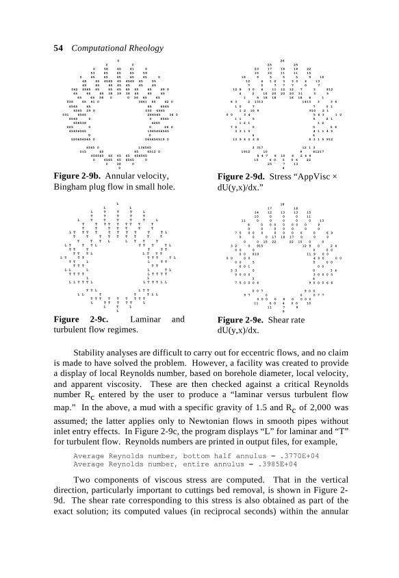
54 Computational Rheology 0 0 0 0 58 60 61 0 53 65 65 65 59 0 65 65 65 65 65 0 48 65 6565 65 6565 65 55 65 65 65 65 65 65 65 042 6565 65 65 65 65 65 65 49 0 65 65 65 38 39 38 65 65 65 65 65 36 0 0 36 65 65 036 65 61 0 3461 65 42 0
6565 65 65 6565 6565 29 0 030 6565 031 6565 266565 34 0 6565 0 0 6565 656538 4265 025 0 0 26 0 65656565 1965656565 0 0 020656565 0 065656519 0
6565 0 136565 015 65 65 6513 0 656565 65 65 65 656565 0 6565 65 6565 0 0 38 0 0
Figure 2-9b. Annular velocity,Bingham plug flow in small hole.
L L L L T T T L T T T T T L T T T T T L T T T T T T T T T T T T T T T T L T T T T T T T T T T L T T T T T T T T T
T T T L L T T T L T T T L T T T T L T T T T T T T T T L L T T T L T T T T T T T L T T L L T T T T T T T L L L L T L T T T T L T T T T L L L L T T T L L T T T L L
T T L L T T L L T T T L L T T T T T T T T T L T T T T T L L T L L
Figure 2-9c. Laminar andturbulent flow regimes.
26 25 25 23 17 18 18 22 15 10 11 11 15 18 9 5 5 5 9 18 12 4 1 2 3 3 0 4 13 7 0 7 7 7 0 7 12 8 3 0 6 11 12 12 7 3 812 4 2 10 20 20 20 11 3 5 1 5 18 18 18 18 6 1 6 3 2 1313 1413 3 3 6
1 0 7 7 0 1 1 2 10 9 910 2 1 0 0 3 4 5 4 3 1 0 1 1 5 5 2 1 1 2 1 1 2 7 5 0 0 5 6 3 3 1 0 4 1 1 4 5 4 4 13 9 4 0 3 8 8 3 1 5 912
2 317 12 1 3 1912 10 9 61217 8 4 7 8 10 6 2 6 9 15 6 0 5 0 6 22 25 7 13 4
Figure 2-9d. Stress “AppVisc ×dU(y,x)/dx.”
18 17 18 14 12 13 13 15 10 0 0 0 11 11 0 0 0 0 0 13 8 0 0 0 0 0 0 0 9 0 0 0 0 0 0 0 7 5 0 0 0 0 0 0 0 0 6 9 0 0 0 17 18 17 0 0 0
0 0 15 22 22 15 0 0 3 2 0 915 12 9 0 2 4 0 0 0 0 0 0 0 0 810 11 9 0 0 0 0 0 0 4 0 0 0 0 0 0 5 5 0 0 0 0 1 0 0 3 3 0 0 3 4 0 0 0 0 3 0 0 0 0 3 4 7 5 0 0 0 6 9 0 0 0 6 6
0 0 7 9 0 0 9 7 0 0 0 7 7 0 0 0 0 8 0 0 0 0 11 0 0 4 0 0 10 11 7 9 9
Figure 2-9e. Shear ratedU(y,x)/dx.
Stability analyses are difficult to carry out for eccentric flows, and no claimis made to have solved the problem. However, a facility was created to providea display of local Reynolds number, based on borehole diameter, local velocity,and apparent viscosity. These are then checked against a critical Reynoldsnumber Rc entered by the user to produce a “laminar versus turbulent flow
map.” In the above, a mud with a specific gravity of 1.5 and Rc of 2,000 was
assumed; the latter applies only to Newtonian flows in smooth pipes withoutinlet entry effects. In Figure 2-9c, the program displays “L” for laminar and “T”for turbulent flow. Reynolds numbers are printed in output files, for example,
Average Reynolds number, bottom half annulus = .3770E+04 Average Reynolds number, entire annulus = .3985E+04
Two components of viscous stress are computed. That in the verticaldirection, particularly important to cuttings bed removal, is shown in Figure 2-9d. The shear rate corresponding to this stress is also obtained as part of theexact solution; its computed values (in reciprocal seconds) within the annular
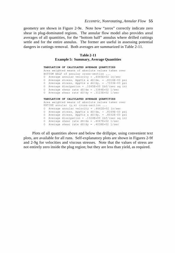
Eccentric, Nonrotating, Annular Flow 55
geometry are shown in Figure 2-9e. Note how “zeros” correctly indicate zeroshear in plug-dominated regions. The annular flow model also provides arealaverages of all quantities, for the “bottom half” annulus where drilled cuttingssettle and for the entire annulus. The former are useful in assessing potentialdangers in cuttings removal. Both averages are summarized in Table 2-11.
Table 2-11Example 5: Summary, Average Quantities
TABULATION OF CALCULATED AVERAGE QUANTITIES Area weighted means of absolute values taken over BOTTOM HALF of annular cross-section ... O Average annular velocity = .4445E+02 in/sec O Average stress, AppVis x dU/dx, = .8316E-03 psi O Average stress, AppVis x dU/dy, = .7333E-03 psi O Average dissipation = .1045E+00 lbf/(sec sq in) O Average shear rate dU/dx = .3384E+02 1/sec O Average shear rate dU/dy = .3123E+02 1/sec
TABULATION OF CALCULATED AVERAGE QUANTITIES Area weighted means of absolute values taken over ENTIRE annular (y,x) cross-section ... O Average annular velocity = .4662E+02 in/sec O Average stress, AppVis x dU/dx, = .8169E-03 psi O Average stress, AppVis x dU/dy, = .8032E-03 psi O Average dissipation = .1324E+00 lbf/(sec sq in) O Average shear rate dU/dx = .4047E+02 1/sec O Average shear rate dU/dy = .4038E+02 1/sec
Plots of all quantities above and below the drillpipe, using convenient textplots, are available for all runs. Self-explanatory plots are shown in Figures 2-9fand 2-9g for velocities and viscous stresses. Note that the values of stress arenot entirely zero inside the plug region; but they are less than yield, as required.
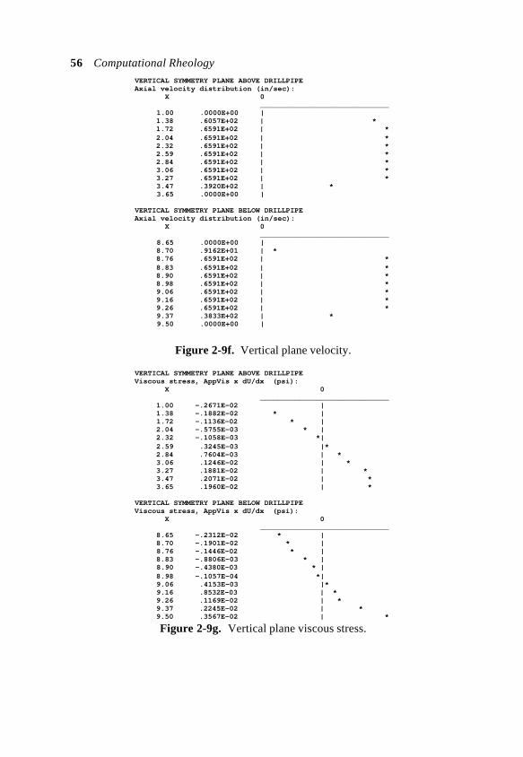
56 Computational Rheology
VERTICAL SYMMETRY PLANE ABOVE DRILLPIPE Axial velocity distribution (in/sec): X 0 ______________________________ 1.00 .0000E+00 | 1.38 .6057E+02 | * 1.72 .6591E+02 | * 2.04 .6591E+02 | * 2.32 .6591E+02 | * 2.59 .6591E+02 | * 2.84 .6591E+02 | * 3.06 .6591E+02 | * 3.27 .6591E+02 | * 3.47 .3920E+02 | * 3.65 .0000E+00 |
VERTICAL SYMMETRY PLANE BELOW DRILLPIPE Axial velocity distribution (in/sec): X 0 ______________________________ 8.65 .0000E+00 | 8.70 .9162E+01 | * 8.76 .6591E+02 | * 8.83 .6591E+02 | * 8.90 .6591E+02 | * 8.98 .6591E+02 | * 9.06 .6591E+02 | * 9.16 .6591E+02 | * 9.26 .6591E+02 | * 9.37 .3833E+02 | * 9.50 .0000E+00 |
Figure 2-9f. Vertical plane velocity.
VERTICAL SYMMETRY PLANE ABOVE DRILLPIPE Viscous stress, AppVis x dU/dx (psi): X 0 ______________________________ 1.00 -.2671E-02 | 1.38 -.1882E-02 * | 1.72 -.1136E-02 * | 2.04 -.5755E-03 * | 2.32 -.1058E-03 *| 2.59 .3245E-03 |* 2.84 .7604E-03 | * 3.06 .1246E-02 | * 3.27 .1881E-02 | * 3.47 .2071E-02 | * 3.65 .1960E-02 | *
VERTICAL SYMMETRY PLANE BELOW DRILLPIPE Viscous stress, AppVis x dU/dx (psi): X 0 ______________________________ 8.65 -.2312E-02 * | 8.70 -.1901E-02 * | 8.76 -.1446E-02 * | 8.83 -.8806E-03 * | 8.90 -.4380E-03 * | 8.98 -.1057E-04 *| 9.06 .4153E-03 |* 9.16 .8532E-03 | * 9.26 .1169E-02 | * 9.37 .2245E-02 | * 9.50 .3567E-02 | *
Figure 2-9g. Vertical plane viscous stress.
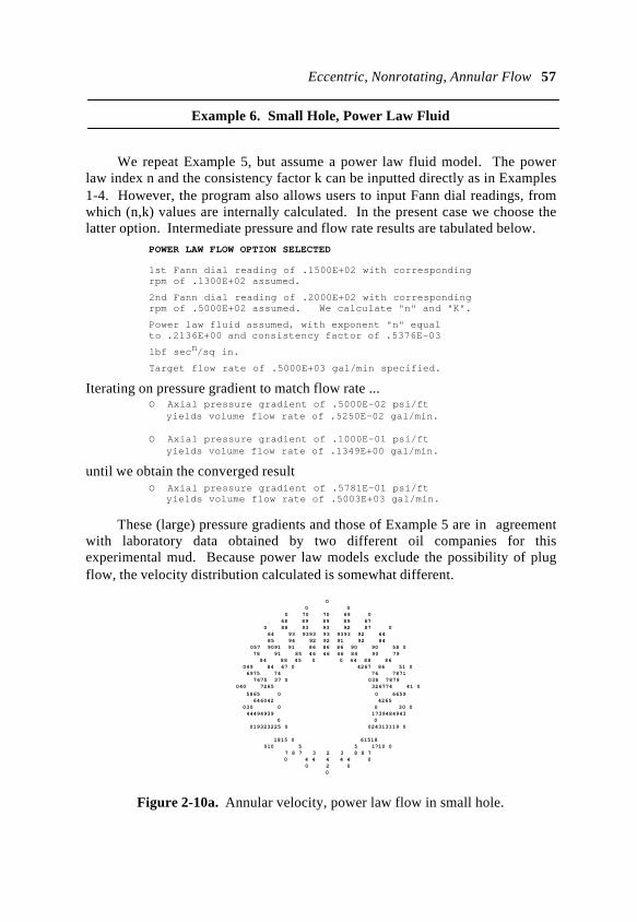
Eccentric, Nonrotating, Annular Flow 57
Example 6. Small Hole, Power Law Fluid
We repeat Example 5, but assume a power law fluid model. The powerlaw index n and the consistency factor k can be inputted directly as in Examples1-4. However, the program also allows users to input Fann dial readings, fromwhich (n,k) values are internally calculated. In the present case we choose thelatter option. Intermediate pressure and flow rate results are tabulated below. POWER LAW FLOW OPTION SELECTED
1st Fann dial reading of .1500E+02 with corresponding rpm of .1300E+02 assumed.
2nd Fann dial reading of .2000E+02 with corresponding rpm of .5000E+02 assumed. We calculate "n" and "K".
Power law fluid assumed, with exponent "n" equal to .2136E+00 and consistency factor of .5376E-03
lbf secn/sq in.
Target flow rate of .5000E+03 gal/min specified.
Iterating on pressure gradient to match flow rate ... O Axial pressure gradient of .5000E-02 psi/ft yields volume flow rate of .5250E-02 gal/min.
O Axial pressure gradient of .1000E-01 psi/ft yields volume flow rate of .1349E+00 gal/min.
until we obtain the converged result O Axial pressure gradient of .5781E-01 psi/ft yields volume flow rate of .5003E+03 gal/min.
These (large) pressure gradients and those of Example 5 are in agreementwith laboratory data obtained by two different oil companies for thisexperimental mud. Because power law models exclude the possibility of plugflow, the velocity distribution calculated is somewhat different.
0 0 0 0 70 70 69 0 68 89 89 89 67 0 88 93 93 92 87 0 64 93 9393 93 9393 92 64 85 94 92 92 91 92 84 057 9091 91 86 86 86 90 90 58 0 78 91 85 46 46 46 84 90 79 84 88 45 0 0 44 88 86 049 84 67 0 4267 86 51 0 6975 74 76 7871 7675 37 0 038 7879 040 7265 326774 41 0
5865 0 0 6659 646042 4265 030 0 0 30 0 44494939 1739484943 0 0 019323225 0 024313119 0
1815 0 61518 010 5 5 1710 0 7 8 7 3 2 3 8 8 7 0 4 4 4 4 4 0 0 2 0 0
Figure 2-10a. Annular velocity, power law flow in small hole.
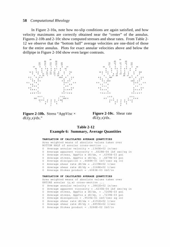
58 Computational Rheology
In Figure 2-10a, note how no-slip conditions are again satisfied, and howvelocity maximums are correctly obtained near the “center” of the annulus.Figures 2-10b and 2-10c show computed stresses and shear rates. From Table 2-12 we observe that the “bottom half” average velocities are one-third of thosefor the entire annulus. Plots for exact annular velocities above and below thedrillpipe in Figure 2-10d show even larger contrasts.
25 24 24 22 14 15 14 22 13 11 11 11 12
17 9 7 7 7 9 17 10 6 3 6 6 6 1 6 10 7 0 9 9 9 0 7 11 6 4 2 9 11 11 11 9 4 711 4 8 11 15 15 15 10 7 4 0 9 14 7 7 14 8 1 0 3 8 11 6 1210 8 3 0 1 1 8 8 1 1 6 9 8 5 5 8 9 6 0 1 7 6 5 6 7 1 0 2 8 3 3 9 2 9 6 2 2 9 2 5 0 0 5 2 6 8 8 1 2 1 8 8 6 2 2 4 8 9 7 0 5 5 0 7 9 8 4
9 0 7 7 0 9 610 7 7 1010 6 10 9 5 6 6 6 1 910 7 7 0 3 0 7 7 6 1 6 1
Figure 2-10b. Stress “AppVisc ×dU(y,x)/dx.”
21 20 20 18 12 12 12 18 11 3 3 3 10
15 3 0 0 0 3 15 9 0 0 0 0 0 0 0 9 2 0 1 1 1 0 2 10 6 0 0 1 4 4 4 1 0 610 1 0 4 19 19 18 4 0 2 0 1 17 28 28 17 1 0 4 2 1 820 14 7 0 2 5 0 0 3 3 0 0 0 1 1013 1410 1 0 0 0 1 2 5 2 2 1 0 1 1 6 7 1 1 1 1 1 1 1 5 4 0 0 4 5 3 2 1 0 2 0 1 2 3 3 3 7 5 2 1 0 5 5 0 1 2 5 7
1 0 5 3 0 1 6 5 1 1 2 4 6 2 1 0 0 0 0 0 1 2 4 0 0 0 0 0 4 2 0 2 0
Figure 2-10c. Shear ratedU(y,x)/dx.
Table 2-12Example 6: Summary, Average Quantities
TABULATION OF CALCULATED AVERAGE QUANTITIES Area weighted means of absolute values taken over BOTTOM HALF of annular cross-section ... O Average annular velocity = .1360E+02 in/sec O Average apparent viscosity = .6028E-04 lbf sec/sq in O Average stress, AppVis x dU/dx, = .6395E-03 psi O Average stress, AppVis x dU/dy, = .6879E-03 psi O Average dissipation = .4688E-01 lbf/(sec sq in) O Average shear rate dU/dx = .2139E+02 1/sec O Average shear rate dU/dy = .3168E+02 1/sec O Average Stokes product = .6083E-03 lbf/in
TABULATION OF CALCULATED AVERAGE QUANTITIES Area weighted means of absolute values taken over ENTIRE annular (y,x) cross-section ... O Average annular velocity = .3841E+02 in/sec O Average apparent viscosity = .6230E-04 lbf sec/sq in O Average stress, AppVis x dU/dx, = .7269E-03 psi O Average stress, AppVis x dU/dy, = .7239E-03 psi O Average dissipation = .9535E-01 lbf/(sec sq in) O Average shear rate dU/dx = .4191E+02 1/sec O Average shear rate dU/dy = .4855E+02 1/sec O Average Stokes product = .3266E-02 lbf/in

Eccentric, Nonrotating, Annular Flow 59 VERTICAL SYMMETRY PLANE ABOVE DRILLPIPE Axial velocity distribution (in/sec): X 0 ______________________________ 1.00 .0000E+00 | 1.38 .7068E+02 | * 1.72 .8983E+02 | * 2.04 .9341E+02 | * 2.32 .9361E+02 | * 2.59 .9353E+02 | * 2.84 .9219E+02 | * 3.06 .8696E+02 | * 3.27 .7368E+02 | * 3.47 .4686E+02 | * 3.65 .0000E+00 |
VERTICAL SYMMETRY PLANE BELOW DRILLPIPE Axial velocity distribution (in/sec): X 0 ______________________________ 8.65 .0000E+00 | 8.70 .1642E+01 | * 8.76 .2797E+01 | * 8.83 .3560E+01 | * 8.90 .4019E+01 | * 8.98 .4244E+01 | * 9.06 .4265E+01 | * 9.16 .4036E+01 | * 9.26 .3419E+01 | * 9.37 .2188E+01 | * 9.50 .0000E+00 |
Figure 2-10d. Vertical plane velocity.
Example 7. Large Hole, Bingham Plastic
We next consider a 2.5-inch-radius drillpipe residing in a 6.1-inch-radiusborehole. The pipe is displaced halfway down by 1.80 inches. Again, thecomputer code produces a boundary conforming grid system for exactcalculations. This mesh is shown in Figure 2-11a.
11 11 11 11 11 10 10 10 11 10 9 10 11
9 9 10 9 8 8 8 9 10 11 9 8 7 7 7 8 9 11 10 7 6 6 6 7 10 8 6 5 5 5 6 8 11 9 7 5 4 4 4 5 7 9 11 10 8 6 4 3 3 3 4 6 8 10 9 7 6 4 3 2 2 1 2 2 3 4 7 9 8 5 4 3 1 1 3 4 5 8 1110 7 6 3 2 1 1 3 6 7 10 11 9 8 5 4 3 1 1 4 5 8 9 7 2 2 7 1110 5 4 2 2 4 5 1011 9 8 7 6 6 7 8 9 4 3 2 4 1110 9 8 7 6 4 2 1 4 5 7 8 91011 3 1 1 3 9 8 6 4 3 2 2 3 4 6 8 9 1110 6 4 4 4 5 6 1011 10 8 7 5 6 5 7 810 11 9 9 9 11 1110 10 11 11
Figure 2-11a. Mesh system forlarge hole.
0 0 0 0 0 22 22 22 0 22 22 22 0
22 22 22 22 22 22 22 22 22 0 22 22 22 22 22 22 22 0 22 22 22 22 22 22 22 22 22 22 2222 22 22 0 22 22 22 22 2222 22 22 22 0 22 22 22 22 22 2222 22 22 22 22 22 2222 22222222 022222222 22 22 22 222222 0 0 222222 22 022 2222 2222 0 0 22 2222 22 0 2222 222222 0 0 2222 2222 22 22 22 22 022 222222 222222 22 0 22222222 22222222 2222 2222 022222222222222 0222222222222 0 22 0 022 222222222222 222222222222 022 22 22 2222 2222 22 0 2222 2222 222222 2222 0 22 22 22 0 022 22 0 0
Figure 2-11b. Annular velocity,Bingham plug flow in large hole.
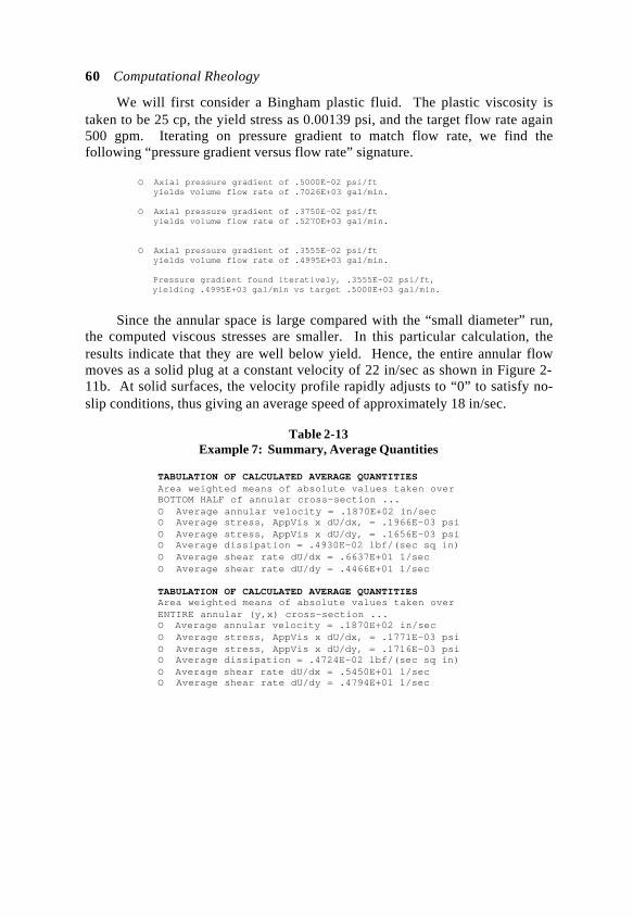
60 Computational Rheology
We will first consider a Bingham plastic fluid. The plastic viscosity istaken to be 25 cp, the yield stress as 0.00139 psi, and the target flow rate again500 gpm. Iterating on pressure gradient to match flow rate, we find thefollowing “pressure gradient versus flow rate” signature.
O Axial pressure gradient of .5000E-02 psi/ft yields volume flow rate of .7026E+03 gal/min.
O Axial pressure gradient of .3750E-02 psi/ft yields volume flow rate of .5270E+03 gal/min.
O Axial pressure gradient of .3555E-02 psi/ft yields volume flow rate of .4995E+03 gal/min.
Pressure gradient found iteratively, .3555E-02 psi/ft, yielding .4995E+03 gal/min vs target .5000E+03 gal/min.
Since the annular space is large compared with the “small diameter” run,the computed viscous stresses are smaller. In this particular calculation, theresults indicate that they are well below yield. Hence, the entire annular flowmoves as a solid plug at a constant velocity of 22 in/sec as shown in Figure 2-11b. At solid surfaces, the velocity profile rapidly adjusts to “0” to satisfy no-slip conditions, thus giving an average speed of approximately 18 in/sec.
Table 2-13Example 7: Summary, Average Quantities
TABULATION OF CALCULATED AVERAGE QUANTITIES Area weighted means of absolute values taken over BOTTOM HALF of annular cross-section ... O Average annular velocity = .1870E+02 in/sec O Average stress, AppVis x dU/dx, = .1966E-03 psi O Average stress, AppVis x dU/dy, = .1656E-03 psi O Average dissipation = .4930E-02 lbf/(sec sq in) O Average shear rate dU/dx = .6637E+01 1/sec O Average shear rate dU/dy = .4466E+01 1/sec
TABULATION OF CALCULATED AVERAGE QUANTITIES Area weighted means of absolute values taken over ENTIRE annular (y,x) cross-section ... O Average annular velocity = .1870E+02 in/sec O Average stress, AppVis x dU/dx, = .1771E-03 psi O Average stress, AppVis x dU/dy, = .1716E-03 psi O Average dissipation = .4724E-02 lbf/(sec sq in) O Average shear rate dU/dx = .5450E+01 1/sec O Average shear rate dU/dy = .4794E+01 1/sec
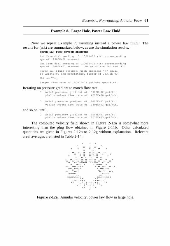
Eccentric, Nonrotating, Annular Flow 61
Example 8. Large Hole, Power Law Fluid
Now we repeat Example 7, assuming instead a power law fluid. Theresults for (n,k) are summarized below, as are the simulation results. POWER LAW FLOW OPTION SELECTED 1st Fann dial reading of .1500E+02 with corresponding rpm of .1300E+02 assumed.
2nd Fann dial reading of .2000E+02 with corresponding rpm of .5000E+02 assumed. We calculate "n" and "k."
Power law fluid assumed, with exponent "n" equal to .2136E+00 and consistency factor of .5376E-03
lbf secn/sq in.
Target flow rate of .5000E+03 gal/min specified.
Iterating on pressure gradient to match flow rate ... O Axial pressure gradient of .5000E-02 psi/ft yields volume flow rate of .6528E+00 gal/min.
O Axial pressure gradient of .1000E-01 psi/ft yields volume flow rate of .1593E+02 gal/min.
and so on, until, O Axial pressure gradient of .2094E-01 psi/ft yields volume flow rate of .5039E+03 gal/min.
The computed velocity field shown in Figure 2-12a is somewhat moreinteresting than the plug flow obtained in Figure 2-11b. Other calculatedquantities are given in Figures 2-12b to 2-12g without explanation. Relevantareal averages are listed in Table 2-14.
0 0 0 0 0 28 28 28 0 27 32 27 0 32 32 26 32 32 32 32 32 26 0 31 32 32 32 32 32 31 0 24 32 32 32 32 32 24 32 32 31 3131 32 32 0 30 32 31 29 2929 31 32 30 0 22 31 32 28 23 2323 28 32 31 22 28 3131 27231414 014142327 31 28 29 292622 0 0 222629 30 018 3029 2112 0 0 21 2930 19 0
2527 272418 0 0 2427 2725 27 10 11 27 015 2421 9 92124 15 0 20222221 21222221 1712 717 0111517171512 5 0121517171511 0 6 0 0 6 101111 8 4 2 2 4 8111110 0 7 7 3 3 3 6 7 7 0 4 7 4 4 4 4 4 7 4 0 3 3 3 0 0 2 2 0 0
Figure 2-12a. Annular velocity, power law flow in large hole.
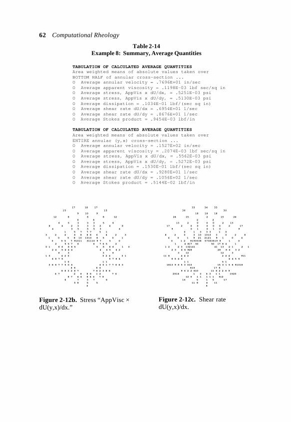
62 Computational Rheology
Table 2-14Example 8: Summary, Average Quantities
TABULATION OF CALCULATED AVERAGE QUANTITIES Area weighted means of absolute values taken over BOTTOM HALF of annular cross-section ... O Average annular velocity = .7696E+01 in/sec O Average apparent viscosity = .1198E-03 lbf sec/sq in O Average stress, AppVis x dU/dx, = .5251E-03 psi O Average stress, AppVis x dU/dy, = .5130E-03 psi O Average dissipation = .1034E-01 lbf/(sec sq in) O Average shear rate dU/dx = .6954E+01 1/sec O Average shear rate dU/dy = .8676E+01 1/sec O Average Stokes product = .9454E-03 lbf/in
TABULATION OF CALCULATED AVERAGE QUANTITIES Area weighted means of absolute values taken over ENTIRE annular (y,x) cross-section ... O Average annular velocity = .1527E+02 in/sec O Average apparent viscosity = .2074E-03 lbf sec/sq in O Average stress, AppVis x dU/dx, = .5562E-03 psi O Average stress, AppVis x dU/dy, = .5272E-03 psi O Average dissipation = .1530E-01 lbf/(sec sq in) O Average shear rate dU/dx = .9280E+01 1/sec O Average shear rate dU/dy = .1056E+02 1/sec O Average Stokes product = .5144E-02 lbf/in
17 18 17 15 15 9 10 9
12 8 6 8 12 6 6 6 5 3 3 3 5 6 8 4 2 3 3 3 2 4 8 4 3 5 5 5 3 4 1 5 7 7 7 5 1 3 2 4 6 8 8 8 6 4 2 3 1 0 5 8 10 1010 8 5 0 1 0 5 5 7 91011 61110 9 7 5 0 2 5 5 7 6 6 7 5 5 2 0 1 6 6 6 6 5 5 6 6 6 1 0 2 4 5 4 4 4 4 4 5 4 2 6 3 3 6 1 3 4 2 0 0 2 4 3 1 4 6 7 5 5 7 6 4 1 0 1 1 3 6 6 7 7 5 0 4 4 0 1 7 7 6 6 3 4 6 6 4 8 8 3 2 6 7 7 6 2 3 8 8 4 7 2 6 8 6 1 2 7 4 8 7 4 4 8 4 4 7 8 6 7 3 7 6 5 8 5 5 4
Figure 2-12b. Stress “AppVisc ×dU(y,x)/dx.”
33 34 33 30 30 18 18 18
24 15 2 15 24 2 2 13 2 0 0 0 2 13 17 2 0 0 0 0 0 2 17 9 0 1 0 1 0 9 0 1 3 3 3 1 0 8 2 0 3 10 1010 3 0 2 8 4 0 1 9 21 2121 9 1 0 4 0 1 2 9193538 57383519 9 1 0 1 4 817 50 50 17 8 4 1 1 2 2 3 132141 41 13 2 1 2 1 2 3 4 6 928 28 6 4 3 2 3 12 12 3 11 8 4 4 2 2 4 4 911 6 5 4 4 4 4 5 6 1 1 5 1 1813 9 6 5 3 010 15 0 1 5 6 91318 615 17 6 9 6 2 2 610 11 6 2 2 6 9 2014 1 3 4 3 1 1 1520 12 5 1 1 1 1 1 512 15 5 1 5 17 11 8 4 11 6
Figure 2-12c. Shear ratedU(y,x)/dx.
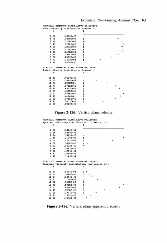
Eccentric, Nonrotating, Annular Flow 63 VERTICAL SYMMETRY PLANE ABOVE DRILLPIPE Axial velocity distribution (in/sec): X 0 ______________________________ 1.00 .0000E+00 | 1.95 .2859E+02 | * 2.76 .3260E+02 | * 3.45 .3272E+02 | * 4.05 .3271E+02 | * 4.58 .3258E+02 | * 5.03 .3175E+02 | * 5.44 .2928E+02 | * 5.80 .2399E+02 | * 6.12 .1463E+02 | * 6.40 .0000E+00 |
VERTICAL SYMMETRY PLANE BELOW DRILLPIPE Axial velocity distribution (in/sec): X 0 ______________________________ 11.40 .0000E+00 | 11.51 .1649E+01 | * 11.64 .2890E+01 | * 11.77 .3762E+01 | * 11.92 .4313E+01 | * 12.09 .4595E+01 | * 12.27 .4640E+01 | * 12.47 .4404E+01 | * 12.69 .3741E+01 | * 12.93 .2403E+01 | * 13.20 .0000E+00 |
Figure 2-12d. Vertical plane velocity.
VERTICAL SYMMETRY PLANE ABOVE DRILLPIPE Apparent viscosity distribution (lbf sec/sq in): X 0 ______________________________ 1.00 .5410E-04 | 1.95 .5410E-04 | 2.76 .2425E-03 * 3.45 .3657E-02 | * 4.05 .2792E-02 | * 4.58 .5468E-03 | * 5.03 .1873E-03 * 5.44 .8667E-04 | 5.80 .4789E-04 | 6.12 .2969E-04 | 6.40 .1149E-04 |
VERTICAL SYMMETRY PLANE BELOW DRILLPIPE Apparent viscosity distribution (lbf sec/sq in): X 0 ______________________________ 11.40 .6464E-04 | * 11.51 .1046E-03 | * 11.64 .1446E-03 | * 11.77 .2176E-03 | * 11.92 .3630E-03 | * 12.09 .5925E-03 | * 12.27 .5426E-03 | * 12.47 .3238E-03 | * 12.69 .1997E-03 | * 12.93 .1332E-03 | * 13.20 .6672E-04 | *
Figure 2-12e. Vertical plane apparent viscosity.
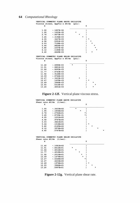
64 Computational Rheology
VERTICAL SYMMETRY PLANE ABOVE DRILLPIPE Viscous stress, AppVis x dU/dx (psi): X 0 ______________________________ 1.00 -.1857E-02 | 1.95 -.1003E-02 * | 2.76 -.6673E-03 * | 3.45 -.3194E-03 * | 4.05 .3437E-03 | * 4.58 .5351E-03 | * 5.03 .7158E-03 | * 5.44 .8824E-03 | * 5.80 .1037E-02 | * 6.12 .1180E-02 | * 6.40 .6649E-03 | *
VERTICAL SYMMETRY PLANE BELOW DRILLPIPE Viscous stress, AppVis x dU/dx (psi): X 0 ______________________________ 11.40 -.6990E-03 * | 11.51 -.8801E-03 | 11.64 -.8693E-03 | 11.77 -.8743E-03 | 11.92 -.9128E-03 | 12.09 -.8764E-03 | 12.27 -.3433E-03 * | 12.47 .1435E-03 | * 12.69 .3946E-03 | * 12.93 .5310E-03 | * 13.20 .4001E-03 | *
Figure 2-12f. Vertical plane viscous stress.
VERTICAL SYMMETRY PLANE ABOVE DRILLPIPE Shear rate dU/dx (1/sec): X 0 ______________________________ 1.00 -.3433E+02 * | 1.95 -.1854E+02 * | 2.76 -.2752E+01 *| 3.45 -.8735E-01 *| 4.05 .1231E+00 | 4.58 .9787E+00 | 5.03 .3821E+01 | 5.44 .1018E+02 | * 5.80 .2165E+02 | * 6.12 .3976E+02 | * 6.40 .5787E+02 | *
VERTICAL SYMMETRY PLANE BELOW DRILLPIPE Shear rate dU/dx (1/sec): X 0 ______________________________ 11.40 -.1081E+02 | 11.51 -.8412E+01 * | 11.64 -.6012E+01 * | 11.77 -.4018E+01 * | 11.92 -.2515E+01 * | 12.09 -.1479E+01 * | 12.27 -.6328E+00 *| 12.47 .4433E+00 | 12.69 .1976E+01 | * 12.93 .3986E+01 | * 13.20 .5997E+01 | *
Figure 2-12g. Vertical plane shear rate.
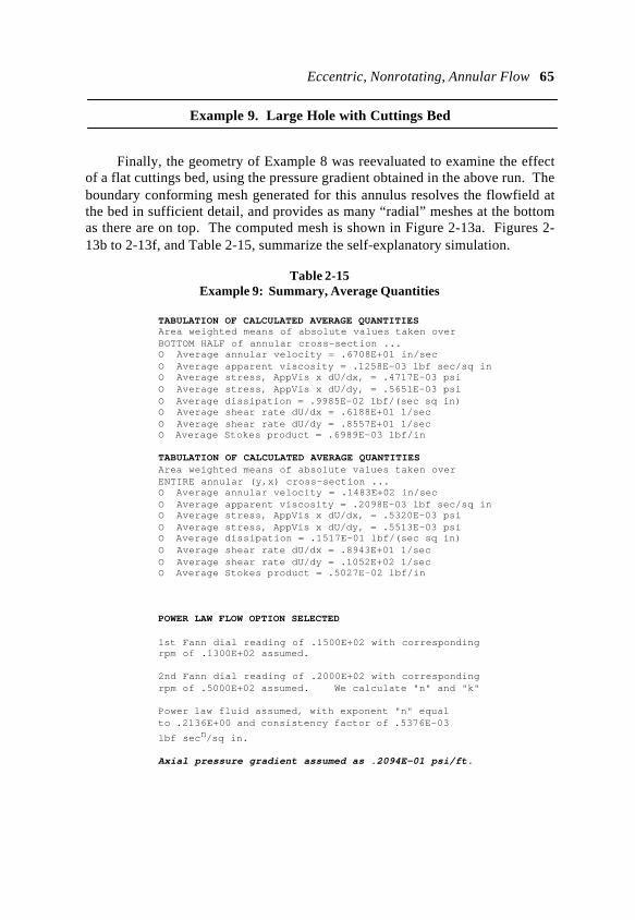
Eccentric, Nonrotating, Annular Flow 65
Example 9. Large Hole with Cuttings Bed
Finally, the geometry of Example 8 was reevaluated to examine the effectof a flat cuttings bed, using the pressure gradient obtained in the above run. Theboundary conforming mesh generated for this annulus resolves the flowfield atthe bed in sufficient detail, and provides as many “radial” meshes at the bottomas there are on top. The computed mesh is shown in Figure 2-13a. Figures 2-13b to 2-13f, and Table 2-15, summarize the self-explanatory simulation.
Table 2-15Example 9: Summary, Average Quantities
TABULATION OF CALCULATED AVERAGE QUANTITIES Area weighted means of absolute values taken over BOTTOM HALF of annular cross-section ... O Average annular velocity = .6708E+01 in/sec O Average apparent viscosity = .1258E-03 lbf sec/sq in O Average stress, AppVis x dU/dx, = .4717E-03 psi O Average stress, AppVis x dU/dy, = .5651E-03 psi O Average dissipation = .9985E-02 lbf/(sec sq in) O Average shear rate dU/dx = .6188E+01 1/sec O Average shear rate dU/dy = .8557E+01 1/sec O Average Stokes product = .6989E-03 lbf/in
TABULATION OF CALCULATED AVERAGE QUANTITIES Area weighted means of absolute values taken over ENTIRE annular (y,x) cross-section ... O Average annular velocity = .1483E+02 in/sec O Average apparent viscosity = .2098E-03 lbf sec/sq in O Average stress, AppVis x dU/dx, = .5320E-03 psi O Average stress, AppVis x dU/dy, = .5513E-03 psi O Average dissipation = .1517E-01 lbf/(sec sq in) O Average shear rate dU/dx = .8943E+01 1/sec O Average shear rate dU/dy = .1052E+02 1/sec O Average Stokes product = .5027E-02 lbf/in
POWER LAW FLOW OPTION SELECTED
1st Fann dial reading of .1500E+02 with corresponding rpm of .1300E+02 assumed.
2nd Fann dial reading of .2000E+02 with corresponding rpm of .5000E+02 assumed. We calculate "n" and "k"
Power law fluid assumed, with exponent "n" equal to .2136E+00 and consistency factor of .5376E-03
lbf secn/sq in.
Axial pressure gradient assumed as .2094E-01 psi/ft.
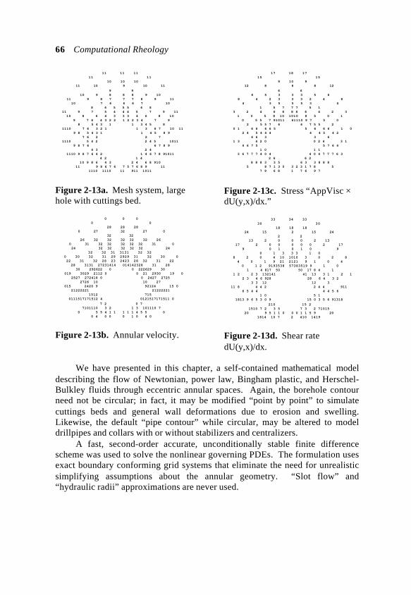
66 Computational Rheology
11 11 11 11 11 10 10 10 11 10 9 10 11
9 9 10 9 8 8 8 9 10 11 9 8 7 7 7 8 9 11 10 7 6 6 6 7 10 8 6 5 5 5 6 8 11 9 7 5 4 4 4 5 7 9 11 10 8 6 4 3 3 3 4 6 8 10 9 7 6 4 3 2 2 1 2 2 3 4 7 9 8 5 4 3 1 1 3 4 5 8 1110 7 6 3 2 1 1 3 6 7 10 11 9 8 5 4 3 1 1 4 5 8 9 7 6 2 2 7 1110 5 4 2 2 4 5 1011 9 8 7 6 6 7 8 9 4 3 2 4 1110 9 8 7 6 4 2 1 4 6 7 8 91011 4 2 1 4 10 9 8 6 4 3 2 4 6 8 910 11 9 8 6 7 6 7 5 7 6 8 9 11 1110 1110 11 911 1011
Figure 2-13a. Mesh system, largehole with cuttings bed.
0 0 0 0 0 28 28 28 0 27 32 27 0 32 32 26 32 32 32 32 32 26 0 31 32 32 32 32 32 31 0 24 32 32 32 32 32 24 32 32 31 3131 32 32 0 30 32 31 29 2929 31 32 30 0 22 31 32 28 23 2423 28 32 31 22 28 3131 27231414 014142328 31 28 30 292622 0 0 222629 30 019 3029 2112 0 0 21 2930 19 0 2527 272418 0 0 2427 2725 2726 10 10 27 015 2420 9 92124 15 0 21222221 21222221 1512 715 0111517171512 4 0121517171511 0
7 2 0 7 7101110 3 2 1 3 101110 7 0 5 5 4 1 1 1 1 1 4 5 5 0 0 4 0 0 0 1 0 4 0
Figure 2-13b. Annular velocity.
17 18 17 15 15 9 10 9 12 8 6 8 12
6 6 6 5 3 3 3 5 6 8 4 2 3 3 3 2 4 8 4 3 5 5 5 3 4 1 5 7 7 7 5 1 3 2 4 6 8 8 8 6 4 2 3 1 0 5 8 10 1010 8 5 0 1 0 5 5 7 91011 61110 9 7 5 0 2 5 5 7 6 6 7 5 5 2 0 1 6 6 6 6 5 5 6 6 6 1 0 2 4 5 4 4 4 4 4 5 4 2 6 6 3 3 6 1 3 4 2 0 0 2 4 3 1 4 6 7 5 5 7 6 4 1 0 1 1 3 6 7 7 7 4 0 4 4 0 4 7 7 7 6 3 2 6 6 2 8 8 8 3 3 5 6 3 3 8 8 8 5 8 7 1 3 0 3 2 3 1 7 8 5 7 9 6 8 1 7 6 9 7
Figure 2-13c. Stress “AppVisc ×dU(y,x)/dx.”
33 34 33 30 30 18 18 18 24 15 2 15 24 2 2 13 2 0 0 0 2 13 17 2 0 0 0 0 0 2 17 9 0 1 0 1 0 9 0 1 3 3 3 1 0 8 2 0 4 10 1010 3 0 2 8 4 0 1 9 21 2121 9 1 0 4 0 1 2 9193538 57383519 9 1 0 1 4 817 50 50 17 8 4 1 1 2 2 3 132141 41 13 3 1 2 1 2 3 4 6 928 28 6 4 3 2 3 3 12 12 3 11 8 4 4 2 2 4 4 911 6 5 4 4 4 4 5 6 1 0 5 1 1813 9 6 5 3 0 9 15 0 3 5 6 91318
210 15 2 1510 7 2 3 5 7 3 2 71015 20 9 5 1 1 0 0 0 1 1 5 9 20 1814 10 7 2 410 1419
Figure 2-13d. Shear ratedU(y,x)/dx.
We have presented in this chapter, a self-contained mathematical modeldescribing the flow of Newtonian, power law, Bingham plastic, and Herschel-Bulkley fluids through eccentric annular spaces. Again, the borehole contourneed not be circular; in fact, it may be modified “point by point” to simulatecuttings beds and general wall deformations due to erosion and swelling.Likewise, the default “pipe contour” while circular, may be altered to modeldrillpipes and collars with or without stabilizers and centralizers.
A fast, second-order accurate, unconditionally stable finite differencescheme was used to solve the nonlinear governing PDEs. The formulation usesexact boundary conforming grid systems that eliminate the need for unrealisticsimplifying assumptions about the annular geometry. “Slot flow” and“hydraulic radii” approximations are never used.
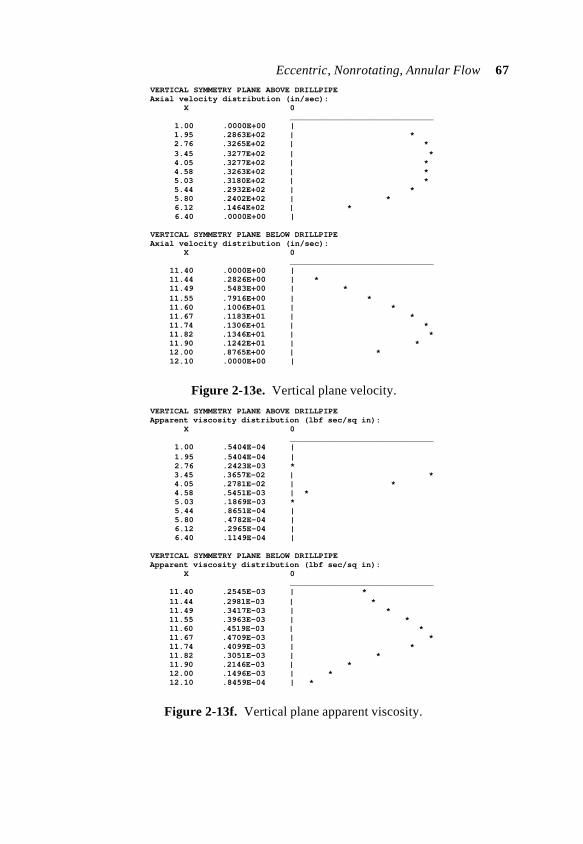
Eccentric, Nonrotating, Annular Flow 67 VERTICAL SYMMETRY PLANE ABOVE DRILLPIPE Axial velocity distribution (in/sec): X 0 ______________________________ 1.00 .0000E+00 | 1.95 .2863E+02 | * 2.76 .3265E+02 | * 3.45 .3277E+02 | * 4.05 .3277E+02 | * 4.58 .3263E+02 | * 5.03 .3180E+02 | * 5.44 .2932E+02 | * 5.80 .2402E+02 | * 6.12 .1464E+02 | * 6.40 .0000E+00 |
VERTICAL SYMMETRY PLANE BELOW DRILLPIPE Axial velocity distribution (in/sec): X 0 ______________________________ 11.40 .0000E+00 | 11.44 .2826E+00 | * 11.49 .5483E+00 | * 11.55 .7916E+00 | * 11.60 .1006E+01 | * 11.67 .1183E+01 | * 11.74 .1306E+01 | * 11.82 .1346E+01 | * 11.90 .1242E+01 | * 12.00 .8765E+00 | * 12.10 .0000E+00 |
Figure 2-13e. Vertical plane velocity.
VERTICAL SYMMETRY PLANE ABOVE DRILLPIPE Apparent viscosity distribution (lbf sec/sq in): X 0 ______________________________ 1.00 .5404E-04 | 1.95 .5404E-04 | 2.76 .2423E-03 * 3.45 .3657E-02 | * 4.05 .2781E-02 | * 4.58 .5451E-03 | * 5.03 .1869E-03 * 5.44 .8651E-04 | 5.80 .4782E-04 | 6.12 .2965E-04 | 6.40 .1149E-04 |
VERTICAL SYMMETRY PLANE BELOW DRILLPIPE Apparent viscosity distribution (lbf sec/sq in): X 0 ______________________________ 11.40 .2545E-03 | * 11.44 .2981E-03 | * 11.49 .3417E-03 | * 11.55 .3963E-03 | * 11.60 .4519E-03 | * 11.67 .4709E-03 | * 11.74 .4099E-03 | * 11.82 .3051E-03 | * 11.90 .2146E-03 | * 12.00 .1496E-03 | * 12.10 .8459E-04 | *
Figure 2-13f. Vertical plane apparent viscosity.
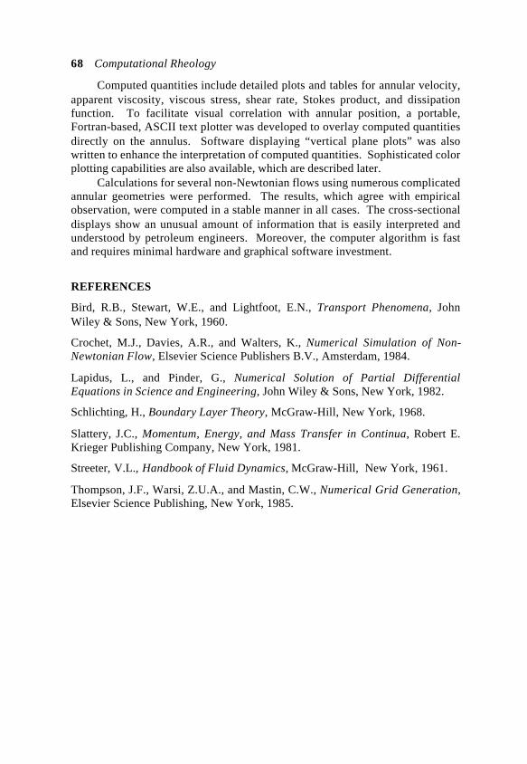
68 Computational Rheology
Computed quantities include detailed plots and tables for annular velocity,apparent viscosity, viscous stress, shear rate, Stokes product, and dissipationfunction. To facilitate visual correlation with annular position, a portable,Fortran-based, ASCII text plotter was developed to overlay computed quantitiesdirectly on the annulus. Software displaying “vertical plane plots” was alsowritten to enhance the interpretation of computed quantities. Sophisticated colorplotting capabilities are also available, which are described later.
Calculations for several non-Newtonian flows using numerous complicatedannular geometries were performed. The results, which agree with empiricalobservation, were computed in a stable manner in all cases. The cross-sectionaldisplays show an unusual amount of information that is easily interpreted andunderstood by petroleum engineers. Moreover, the computer algorithm is fastand requires minimal hardware and graphical software investment.
REFERENCES
Bird, R.B., Stewart, W.E., and Lightfoot, E.N., Transport Phenomena, JohnWiley & Sons, New York, 1960.
Crochet, M.J., Davies, A.R., and Walters, K., Numerical Simulation of Non-Newtonian Flow, Elsevier Science Publishers B.V., Amsterdam, 1984.
Lapidus, L., and Pinder, G., Numerical Solution of Partial DifferentialEquations in Science and Engineering, John Wiley & Sons, New York, 1982.
Schlichting, H., Boundary Layer Theory, McGraw-Hill, New York, 1968.
Slattery, J.C., Momentum, Energy, and Mass Transfer in Continua, Robert E.Krieger Publishing Company, New York, 1981.
Streeter, V.L., Handbook of Fluid Dynamics, McGraw-Hill, New York, 1961.
Thompson, J.F., Warsi, Z.U.A., and Mastin, C.W., Numerical Grid Generation,Elsevier Science Publishing, New York, 1985.
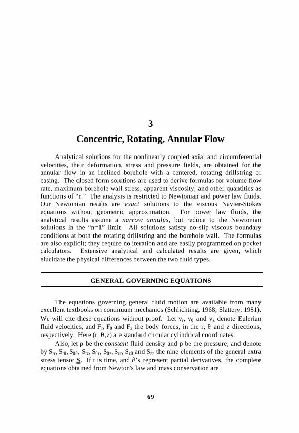
69
3
Concentric, Rotating, Annular Flow
Analytical solutions for the nonlinearly coupled axial and circumferentialvelocities, their deformation, stress and pressure fields, are obtained for theannular flow in an inclined borehole with a centered, rotating drillstring orcasing. The closed form solutions are used to derive formulas for volume flowrate, maximum borehole wall stress, apparent viscosity, and other quantities asfunctions of “r.” The analysis is restricted to Newtonian and power law fluids.Our Newtonian results are exact solutions to the viscous Navier-Stokesequations without geometric approximation. For power law fluids, theanalytical results assume a narrow annulus, but reduce to the Newtoniansolutions in the “n=1” limit. All solutions satisfy no-slip viscous boundaryconditions at both the rotating drillstring and the borehole wall. The formulasare also explicit; they require no iteration and are easily programmed on pocketcalculators. Extensive analytical and calculated results are given, whichelucidate the physical differences between the two fluid types.
GENERAL GOVERNING EQUATIONS
The equations governing general fluid motion are available from manyexcellent textbooks on continuum mechanics (Schlichting, 1968; Slattery, 1981).We will cite these equations without proof. Let vr, vθ and vz denote Eulerianfluid velocities, and Fr, Fθ and Fz the body forces, in the r, θ and z directions,respectively. Here (r, θ ,z) are standard circular cylindrical coordinates.
Also, let ρ be the constant fluid density and p be the pressure; and denoteby Srr, Srθ, Sθθ, Srz, Sθr, Sθz, Szr, Szθ and Szz the nine elements of the general extrastress tensor S. If t is time, and ∂’s represent partial derivatives, the completeequations obtained from Newton's law and mass conservation are

70 Computational Rheology
Momentum equation in r:
ρ (∂vr /∂t + vr ∂vr /∂r + vθ /r ∂vr /∂θ - vθ2/r + vz ∂vr /∂z) = (3-1)
= Fr – ∂p/∂r + 1/r ∂(rSrr)/∂r + 1/r ∂(Srθ)/∂θ + ∂(Srz)/∂z – Sθθ /r
Momentum equation in θ :
ρ (∂vθ /∂t + vr ∂vθ /∂r + vθ /r ∂vθ /∂θ + vrvθ /r + vz ∂vθ /∂z) = (3-2)
= Fθ – 1/r ∂p/∂θ + 1/r 2 ∂(r
2Sθr)/∂r + 1/r ∂(Sθθ)/∂θ + ∂(Sθz)/∂z
Momentum equation in z:
ρ (∂vz /∂t + vr ∂vz /∂r + vθ /r ∂vz /∂θ + vz ∂vz /∂z) = (3-3)
= Fz – ∂p/∂z + 1/r ∂(rSz r)/∂r + 1/r ∂(Sz θ)/∂θ + ∂(Szz)/∂z
Mass continuity equation:
1/r ∂(rvr)/ ∂r + 1/r ∂vθ/∂θ + ∂vz /∂z = 0 (3-4)
These equations apply to all Newtonian and non-Newtonian fluids. Incontinuum mechanics, the most common class of empirical models for isotropic,incompressible fluids assumes that S can be related to the rate of deformationtensor D by a relationship of the form
S = 2 N(Γ) D (3-5)
where the elements of D are
Drr = ∂vr /∂r (3-6)
Dθθ = 1/r ∂vθ/∂θ + vr/r (3-7)
Dzz = ∂vz/∂z (3-8)
Drθ = Dθr = [r ∂(vθ/r)/ ∂r + 1/r ∂vr/∂θ] /2 (3-9)
Drz = Dz r = [∂vr/∂z + ∂vz /∂r] /2 (3-10)
Dθz = Dzθ = [∂vθ/∂z + 1/r ∂vz/∂θ] /2 (3-11)
In Equation 3-5, N(Γ) is the “apparent viscosity function” satisfying
N(Γ) > 0 (3-12)
Γ(r,θ ,z) being the scalar functional of vr, vθ and vz defined by the tensoroperation
Γ = 2 trace (D•D) 1/2 (3-13)
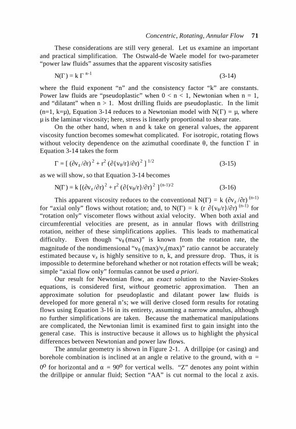
Concentric, Rotating, Annular Flow 71
These considerations are still very general. Let us examine an importantand practical simplification. The Ostwald-de Waele model for two-parameter“power law fluids” assumes that the apparent viscosity satisfies
N(Γ) = k Γ n-1 (3-14)
where the fluid exponent “n” and the consistency factor “k” are constants.Power law fluids are “pseudoplastic” when 0 < n < 1, Newtonian when n = 1,and “dilatant” when n > 1. Most drilling fluids are pseudoplastic. In the limit(n=1, k=µ), Equation 3-14 reduces to a Newtonian model with N(Γ) = µ, whereµ is the laminar viscosity; here, stress is linearly proportional to shear rate.
On the other hand, when n and k take on general values, the apparentviscosity function becomes somewhat complicated. For isotropic, rotating flowswithout velocity dependence on the azimuthal coordinate θ, the function Γ inEquation 3-14 takes the form
Γ = [ (∂vz /∂r) 2 + r2 (∂vθ/r/∂r) 2 ] 1/2 (3-15)
as we will show, so that Equation 3-14 becomes
N(Γ) = k [(∂vz /∂r) 2 + r2 (∂vθ/r/∂r) 2 ] (n-1)/2 (3-16)
This apparent viscosity reduces to the conventional N(Γ) = k (∂vz /∂r) (n-1)
for “axial only” flows without rotation; and, to N(Γ) = k (r ∂vθ/r/∂r) (n-1) for“rotation only” viscometer flows without axial velocity. When both axial andcircumferential velocities are present, as in annular flows with drillstringrotation, neither of these simplifications applies. This leads to mathematicaldifficulty. Even though “vθ (max)” is known from the rotation rate, themagnitude of the nondimensional “vθ (max)/vz(max)” ratio cannot be accuratelyestimated because vz is highly sensitive to n, k, and pressure drop. Thus, it isimpossible to determine beforehand whether or not rotation effects will be weak;simple “axial flow only” formulas cannot be used a priori.
Our result for Newtonian flow, an exact solution to the Navier-Stokesequations, is considered first, without geometric approximation. Then anapproximate solution for pseudoplastic and dilatant power law fluids isdeveloped for more general n’s; we will derive closed form results for rotatingflows using Equation 3-16 in its entirety, assuming a narrow annulus, althoughno further simplifications are taken. Because the mathematical manipulationsare complicated, the Newtonian limit is examined first to gain insight into thegeneral case. This is instructive because it allows us to highlight the physicaldifferences between Newtonian and power law flows.
The annular geometry is shown in Figure 2-1. A drillpipe (or casing) andborehole combination is inclined at an angle α relative to the ground, with α =
0o for horizontal and α = 90o for vertical wells. “Z” denotes any point withinthe drillpipe or annular fluid; Section “AA” is cut normal to the local z axis.
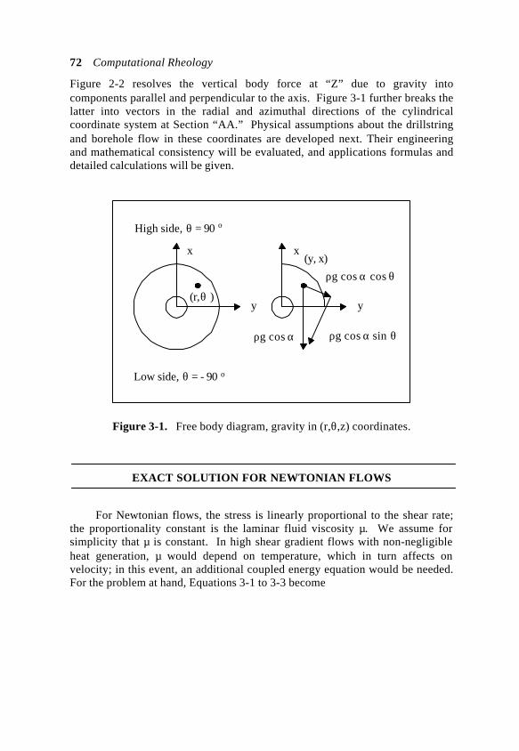
72 Computational Rheology
Figure 2-2 resolves the vertical body force at “Z” due to gravity intocomponents parallel and perpendicular to the axis. Figure 3-1 further breaks thelatter into vectors in the radial and azimuthal directions of the cylindricalcoordinate system at Section “AA.” Physical assumptions about the drillstringand borehole flow in these coordinates are developed next. Their engineeringand mathematical consistency will be evaluated, and applications formulas anddetailed calculations will be given.
x x
y y
High side, θ = 90 o
Low side, θ = - 90 o
(r,θ )
(y, x)
ρg cos α cos θ
ρg cos α sin θρg cos α
Figure 3-1. Free body diagram, gravity in (r,θ,z) coordinates.
EXACT SOLUTION FOR NEWTONIAN FLOWS
For Newtonian flows, the stress is linearly proportional to the shear rate;the proportionality constant is the laminar fluid viscosity µ. We assume forsimplicity that µ is constant. In high shear gradient flows with non-negligibleheat generation, µ would depend on temperature, which in turn affects onvelocity; in this event, an additional coupled energy equation would be needed.For the problem at hand, Equations 3-1 to 3-3 become
Concentric, Rotating, Annular Flow 73
Momentum equation in r: (3-17)
ρ∂vr /∂t + vr ∂vr /∂r + vθ /r ∂vr /∂θ - vθ2/r + vz ∂vr /∂z = Fr - ∂p/∂r
+ µ∂ 2vr /∂r
2 + 1/r ∂vr /∂r - vr /r 2 + 1/r
2 ∂ 2vr /∂θ
2 - 2/r 2 ∂vθ /∂θ + ∂
2vr /∂z 2
Momentum equation in θ : (3-18)
ρ∂vθ /∂t + vr ∂vθ /∂r + vθ /r ∂vθ /∂θ + vrvθ /r + vz ∂vθ /∂z = Fθ - 1/r ∂p/∂θ+ µ∂
2vθ /∂r 2 + 1/r ∂vθ /∂r - vθ /r
2 + 1/r 2 ∂
2vθ /∂θ 2 + 2/r
2 ∂vr /∂θ + ∂ 2vθ /∂z
2
Momentum equation in z: (3-19)
ρ∂vz /∂t + vr ∂vz /∂r + vθ /r ∂vz /∂θ + vz ∂vz /∂z = Fz - ∂p/∂z
+ µ∂ 2vz /∂r2 + 1/r ∂vz /∂r + 1/r2 ∂
2vz /∂θ 2 + ∂
2vz /∂z 2
In this section, it is convenient to rewrite Equation 3-4 in the expanded form
Mass continuity equation:
∂vr /∂r + vr /r + 1/r ∂vθ /∂θ + ∂vz /∂z = 0 (3-20)
Now consider the free body diagrams in Figures 2-1, 2-2 and 3-1. Figure2-1 shows a straight borehole with a centered, rotating drillstring inclined at anangle α relative to the ground. Figure 2-2, referring to this geometry, resolvesthe gravity vector g into components parallel and perpendicular to the hole axis.Figure 3-1 applies to the circular cross-section AA in Figure 2-1 and introduces
local cylindrical coordinates (r, θ). The “low side, θ = - 90o” marks the positionwhere cuttings beds would normally form. The force ρg cos α of Figure 2-2 isresolved into orthogonal components ρg cos α sin θ and ρ g cos α cos θ.
Physical assumptions about the flow are now given. First, it is expectedthat at any section AA along the borehole axis z, the velocity fields will appearto be the same; they are invariant, so z derivatives of vr, vθ and vz vanish. Also,since the drillpipe and borehole walls are assumed to be impermeable, vr = 0throughout (in formation invasion modeling, this would not apply). While wedo have pipe rotation, the use of circular cylindrical coordinates (with constantvθ at the drillstring) renders the mathematical formulation steady. Thus, all timederivatives vanish. These assumptions imply that
- ρ vθ2/r = Fr - ∂p/∂r - 2µ /r
2 ∂vθ/∂θ (3-21)
ρ vθ/r ∂vθ/∂θ = Fθ - 1/r ∂p/∂θ (3-22)
+ µ∂ 2vθ /∂r
2 + 1/r ∂vθ /∂r - vθ/r 2 + 1/r
2 ∂ 2vθ /∂θ
2
ρ vθ /r ∂vz /∂θ = Fz - ∂p/∂z (3-23)
+ µ∂ 2vz /∂r2 + 1/r ∂vz /∂r + 1/r2 ∂
2vz /∂θ 2
∂ vθ /∂θ = 0 (3-24)
74 Computational Rheology
Equation 3-24 is useful in simplifying Equations 3-21 to 3-23 further. Westraightforwardly obtain
ρ vθ2/r = ρ g cos α sin θ + ∂p/∂r (3-25)
0 = - ρ g cos α cos θ - 1/r ∂p/∂θ (3-26)
+ µ∂ 2vθ /∂r
2 + 1/r ∂vθ /∂r - vθ /r 2
ρ vθ /r ∂vz /∂θ = ρ g sin α - ∂p/∂z (3-27)
+ µ∂ 2vz /∂r2 + 1/r ∂vz /∂r + 1/r2 ∂
2vz /∂θ 2
where we have substituted the body force components of Figures 2-2 and 3-1.Now, since Equation 3-27 does not explicitly contain θ, it follows that vz isindependent of θ. Since we had already shown that there is no z dependence, wefind vz = vz (r) is a function of r only. Equation 3-27 therefore becomes
0 = ρ g sin α - ∂p/∂z + µ∂ 2vz /∂r2 + 1/r ∂vz /∂r (3-28)
To achieve further simplicity, we resolve (without loss of generality) the
pressure p(r,θ,z) into its component dynamic pressures P(z) and P*(r), and itshydrostatic contribution, through the separation of variables
p(r,θ,z) = P(z) + P*(r) + zρg sin α - r ρg cos α sin θ (3-29)
This reduces the governing Navier-Stokes equations to the simpler butmathematically equivalent system
∂ 2vz /∂r2 + 1/r ∂vz /∂r = 1/µ dP(z)/dz = constant (3-30)
∂ 2vθ /∂r
2 + 1/r ∂vθ /∂r - vθ /r 2 = 0 (3-31)
ρ vθ2/r = dP*(r)/dr (3-32)
The separation of variables introduced in Equation 3-29 and the explicitelimination of “g” in Equations 3-30 to 3-32 do not mean that gravity isunimportant; the effects of gravity are simply tracked in the dP(z)/dz term of
Equation 3-30. The function P*(r) will depend on the velocity solution to beobtained. Equations 3-30 to 3-32 are also significant in another respect. Thevelocity fields vz(r) and vθ(r) can be obtained independently of each other,despite the nonlinearity of the Navier-Stokes equations, because Equations 3-30and 3-31 physically uncouple. This decoupling occurs because the nonlinearconvective terms in the original momentum equations identically vanish.Equation 3-32 is only applied (after the fact) to calculate the radial pressure field
P*(r) for use in Equation 3-29. This decoupling applies only to Newtonianflows. For non-Newtonian flows, vz(r) and vθ(r) are strongly coupledmathematically, and different solution strategies are needed.

Concentric, Rotating, Annular Flow 75
This degeneracy with Newtonian flows means that their physical propertieswill be completely different from those of power law fluids. For Newtonianflows, changes in rotation rate will not affect properties in the axial direction, incontrast to non-Newtonian flows. Cuttings transport recommendations deduced,for example, using water as the working medium, cannot be extrapolated togeneral drilling fluids having fractional values of n, using any form ofdimensional analysis. Similarly, observations for power law fluids need notapply to water. This uncoupling was, apparently, first observed by Savins andWallick (1966), and the author is indebted to J. Savins for bringing this earlierresult to his attention. Savins and Wallick noted that in Newtonian flows, nocoupling among the discharge rate, axial pressure gradient, relative motion andtorque through viscosity exists. But we emphasize that the coupling between vz
and vθ reappears in eccentric geometries even for Newtonian flows.Because Equations 3-30 and 3-31 are linear, it is possible to solve for the
complete flowfield using exact classical methods. We will give all requiredsolutions without proof, since they can be verified by direct substitution. For theinside of the drillpipe, the axial flow solution to Equation 3-30 satisfying no-slipconditions at the pipe radius r = RP and zero shear stress at the centerline r = 0 is
vz (r) = (r2 - RP2)/4µ dP(z)/dz (3-33)
Similarly, the rotating flow solution to Equation 3-31 satisfying bounded flow atr = 0 and vθ /r = ω at r = RP is
vθ = ωr (3-34)
This is just the expected equation for solid body rotation. Here, “ω” is aconstant drillstring rotation rate. These velocity results, again, can be linearlysuperposed despite the nonlinearity of the underlying equations.
Now, let L denote the length of the pipe, Pmp be the constant pressure at
the “mudpump” z = 0, and P- be the drillpipe pressure at z = L just upstream ofthe bit nozzles. Direct integration of Equation 3-32 and substitution in Equation3-29 yield the complementary solution for pressure
p(r,θ,z) = Pmp + (P- - Pmp) z/L + ρω2r2/2
+ ρg(z sin α - r cos α sin θ) + constant (3-35)
For the annular region between the rotating drillstring and the stationaryborehole wall, the solution of Equation 3-30 satisfying no-slip conditions at thepipe radius r = RP and at the borehole radius r = RB is
vz (r) = r2 - RP2 + (RB
2 - RP2) (log r/RP)/log RP/RB 1/4µ dP(z)/dz
(3-36)where “log” denotes the natural logarithm. The solution of Equation 3-31satisfying vθ = 0 at r = RB and vθ = ωr at r = RP is
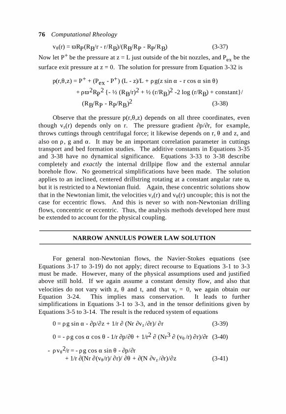
76 Computational Rheology
vθ(r) = ωRP(RB/r - r/RB)/(RB/RP - RP/RB) (3-37)
Now let P+ be the pressure at z = L just outside of the bit nozzles, and Pex be the
surface exit pressure at z = 0. The solution for pressure from Equation 3-32 is
p(r,θ,z) = P+ + (Pex - P+) (L - z)/L + ρg(z sin α - r cos α sin θ)
+ ρω2RP2 - ½ (RB/r)2 + ½ (r/RB)2 -2 log (r/RB) + constant/
(RB/RP - RP/RB)2 (3-38)
Observe that the pressure p(r,θ,z) depends on all three coordinates, eventhough vz(r) depends only on r. The pressure gradient ∂p/∂r, for example,throws cuttings through centrifugal force; it likewise depends on r, θ and z, andalso on ρ, g and α. It may be an important correlation parameter in cuttingstransport and bed formation studies. The additive constants in Equations 3-35and 3-38 have no dynamical significance. Equations 3-33 to 3-38 describecompletely and exactly the internal drillpipe flow and the external annularborehole flow. No geometrical simplifications have been made. The solutionapplies to an inclined, centered drillstring rotating at a constant angular rate ω,but it is restricted to a Newtonian fluid. Again, these concentric solutions showthat in the Newtonian limit, the velocities vz(r) and vθ(r) uncouple; this is not thecase for eccentric flows. And this is never so with non-Newtonian drillingflows, concentric or eccentric. Thus, the analysis methods developed here mustbe extended to account for the physical coupling.
NARROW ANNULUS POWER LAW SOLUTION
For general non-Newtonian flows, the Navier-Stokes equations (seeEquations 3-17 to 3-19) do not apply; direct recourse to Equations 3-1 to 3-3must be made. However, many of the physical assumptions used and justifiedabove still hold. If we again assume a constant density flow, and also thatvelocities do not vary with z, θ and t, and that vr = 0, we again obtain ourEquation 3-24. This implies mass conservation. It leads to furthersimplifications in Equations 3-1 to 3-3, and in the tensor definitions given byEquations 3-5 to 3-14. The result is the reduced system of equations
0 = ρg sin α - ∂p/∂z + 1/r ∂ (Nr ∂vz /∂r)/ ∂r (3-39)
0 = - ρg cos α cos θ - 1/r ∂p/∂θ + 1/r2 ∂ (Nr3 ∂ (vθ /r) ∂r)/∂r (3-40)
- ρvθ2/r = - ρg cos α sin θ - ∂p/∂r
+ 1/r ∂(Nr ∂(vθ/r)/ ∂r)/ ∂θ + ∂(N ∂vz /∂r)/∂z (3-41)
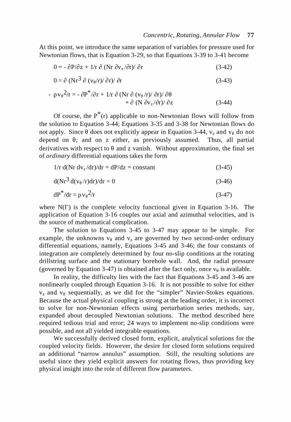
Concentric, Rotating, Annular Flow 77
At this point, we introduce the same separation of variables for pressure used forNewtonian flows, that is Equation 3-29, so that Equations 3-39 to 3-41 become
0 = - ∂P/∂z + 1/r ∂ (Nr ∂vz /∂r)/ ∂r (3-42)
0 = ∂ (Nr3 ∂ (vθ/r)/ ∂r)/ ∂r (3-43)
- ρvθ2/r = - ∂P*/∂r + 1/r ∂ (Nr ∂ (vθ /r)/ ∂r)/ ∂θ
+ ∂ (N ∂vz /∂r)/ ∂z (3-44)
Of course, the P*(r) applicable to non-Newtonian flows will follow fromthe solution to Equation 3-44; Equations 3-35 and 3-38 for Newtonian flows donot apply. Since θ does not explicitly appear in Equation 3-44, vz and vθ do notdepend on θ; and on z either, as previously assumed. Thus, all partialderivatives with respect to θ and z vanish. Without approximation, the final setof ordinary differential equations takes the form
1/r d(Nr dvz /dr)/dr = dP/dz = constant (3-45)
d(Nr3 d(vθ /r)dr)/dr = 0 (3-46)
dP*/dr = ρvθ2/r (3-47)
where N(Γ) is the complete velocity functional given in Equation 3-16. Theapplication of Equation 3-16 couples our axial and azimuthal velocities, and isthe source of mathematical complication.
The solution to Equations 3-45 to 3-47 may appear to be simple. Forexample, the unknowns vθ and vz are governed by two second-order ordinarydifferential equations, namely, Equations 3-45 and 3-46; the four constants ofintegration are completely determined by four no-slip conditions at the rotatingdrillstring surface and the stationary borehole wall. And, the radial pressure(governed by Equation 3-47) is obtained after the fact only, once vθ is available.
In reality, the difficulty lies with the fact that Equations 3-45 and 3-46 arenonlinearly coupled through Equation 3-16. It is not possible to solve for eithervz and vθ sequentially, as we did for the “simpler” Navier-Stokes equations.Because the actual physical coupling is strong at the leading order, it is incorrectto solve for non-Newtonian effects using perturbation series methods, say,expanded about decoupled Newtonian solutions. The method described hererequired tedious trial and error; 24 ways to implement no-slip conditions werepossible, and not all yielded integrable equations.
We successfully derived closed form, explicit, analytical solutions for thecoupled velocity fields. However, the desire for closed form solutions requiredan additional “narrow annulus” assumption. Still, the resulting solutions areuseful since they yield explicit answers for rotating flows, thus providing keyphysical insight into the role of different flow parameters.
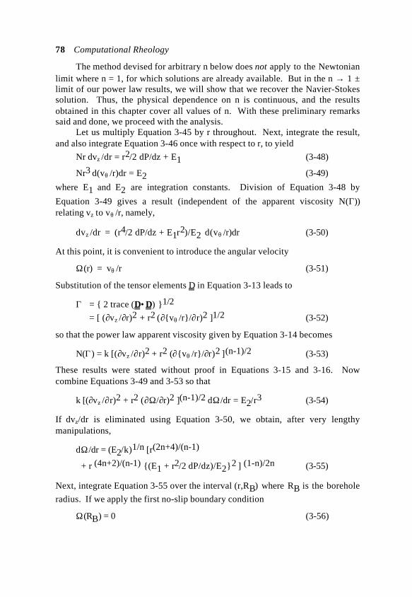
78 Computational Rheology
The method devised for arbitrary n below does not apply to the Newtonianlimit where n = 1, for which solutions are already available. But in the n → 1 ±limit of our power law results, we will show that we recover the Navier-Stokessolution. Thus, the physical dependence on n is continuous, and the resultsobtained in this chapter cover all values of n. With these preliminary remarkssaid and done, we proceed with the analysis.
Let us multiply Equation 3-45 by r throughout. Next, integrate the result,and also integrate Equation 3-46 once with respect to r, to yield
Nr dvz /dr = r2/2 dP/dz + E1 (3-48)
Nr3 d(vθ /r)dr = E2 (3-49)
where E1 and E2 are integration constants. Division of Equation 3-48 by
Equation 3-49 gives a result (independent of the apparent viscosity N(Γ))relating vz to vθ /r, namely,
dvz /dr = (r4/2 dP/dz + E1r2)/E2 d(vθ /r)dr (3-50)
At this point, it is convenient to introduce the angular velocity
Ω(r) = vθ /r (3-51)
Substitution of the tensor elements D in Equation 3-13 leads to
Γ = 2 trace (D•D) 1/2
= [ (∂vz /∂r)2 + r2 (∂vθ /r/∂r)2 ]1/2 (3-52)
so that the power law apparent viscosity given by Equation 3-14 becomes
N(Γ) = k [(∂vz /∂r)2 + r2 (∂vθ /r/∂r)2 ](n-1)/2 (3-53)
These results were stated without proof in Equations 3-15 and 3-16. Nowcombine Equations 3-49 and 3-53 so that
k [(∂vz /∂r)2 + r2 (∂Ω/∂r)2 ](n-1)/2 dΩ/dr = E2/r3 (3-54)
If dvz/dr is eliminated using Equation 3-50, we obtain, after very lengthymanipulations,
dΩ/dr = (E2/k)1/n [r(2n+4)/(n-1)
+ r (4n+2)/(n-1) (E1 + r2/2 dP/dz)/E22 ] (1-n)/2n (3-55)
Next, integrate Equation 3-55 over the interval (r,RB) where RB is the borehole
radius. If we apply the first no-slip boundary condition
Ω(RB) = 0 (3-56)
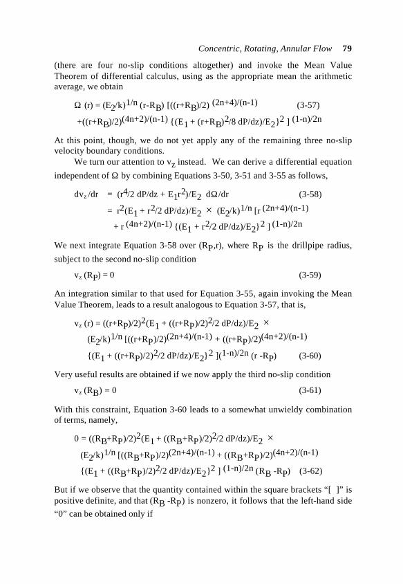
Concentric, Rotating, Annular Flow 79
(there are four no-slip conditions altogether) and invoke the Mean ValueTheorem of differential calculus, using as the appropriate mean the arithmeticaverage, we obtain
Ω (r) = (E2/k)1/n (r-RB) [((r+RB)/2) (2n+4)/(n-1) (3-57)
+((r+RB)/2)(4n+2)/(n-1) (E1 + (r+RB)2/8 dP/dz)/E22 ] (1-n)/2n
At this point, though, we do not yet apply any of the remaining three no-slipvelocity boundary conditions.
We turn our attention to vz instead. We can derive a differential equation
independent of Ω by combining Equations 3-50, 3-51 and 3-55 as follows,
dvz /dr = (r4/2 dP/dz + E1r2)/E2 dΩ/dr (3-58)
= r2(E1 + r2/2 dP/dz)/E2 × (E2/k)1/n [r (2n+4)/(n-1)
+ r (4n+2)/(n-1) (E1 + r2/2 dP/dz)/E22 ] (1-n)/2n
We next integrate Equation 3-58 over (RP,r), where RP is the drillpipe radius,
subject to the second no-slip condition
vz (RP) = 0 (3-59)
An integration similar to that used for Equation 3-55, again invoking the MeanValue Theorem, leads to a result analogous to Equation 3-57, that is,
vz (r) = ((r+RP)/2)2(E1 + ((r+RP)/2)2/2 dP/dz)/E2 × (E2/k)1/n [((r+RP)/2)(2n+4)/(n-1) + ((r+RP)/2)(4n+2)/(n-1)
(E1 + ((r+RP)/2)2/2 dP/dz)/E22 ](1-n)/2n (r -RP) (3-60)
Very useful results are obtained if we now apply the third no-slip condition
vz (RB) = 0 (3-61)
With this constraint, Equation 3-60 leads to a somewhat unwieldy combinationof terms, namely,
0 = ((RB+RP)/2)2(E1 + ((RB+RP)/2)2/2 dP/dz)/E2 × (E2/k)1/n [((RB+RP)/2)(2n+4)/(n-1) + ((RB+RP)/2)(4n+2)/(n-1)
(E1 + ((RB+RP)/2)2/2 dP/dz)/E22 ] (1-n)/2n (RB -RP) (3-62)
But if we observe that the quantity contained within the square brackets “[ ]” ispositive definite, and that (RB -RP) is nonzero, it follows that the left-hand side
“0” can be obtained only if
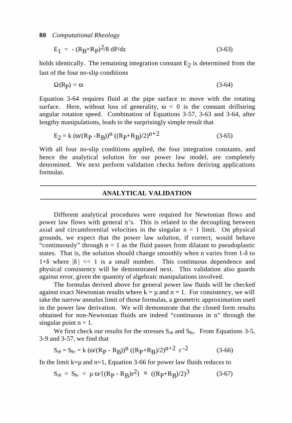
80 Computational Rheology
E1 = - (RB+RP)2/8 dP/dz (3-63)
holds identically. The remaining integration constant E2 is determined from the
last of the four no-slip conditions
Ω(RP) = ω (3-64)
Equation 3-64 requires fluid at the pipe surface to move with the rotatingsurface. Here, without loss of generality, ω < 0 is the constant drillstringangular rotation speed. Combination of Equations 3-57, 3-63 and 3-64, afterlengthy manipulations, leads to the surprisingly simple result that
E2 = k (ω/(RP -RB))n ((RP+RB)/2)n+2 (3-65)
With all four no-slip conditions applied, the four integration constants, andhence the analytical solution for our power law model, are completelydetermined. We next perform validation checks before deriving applicationsformulas.
ANALYTICAL VALIDATION
Different analytical procedures were required for Newtonian flows andpower law flows with general n’s. This is related to the decoupling betweenaxial and circumferential velocities in the singular n = 1 limit. On physicalgrounds, we expect that the power law solution, if correct, would behave“continuously” through n = 1 as the fluid passes from dilatant to pseudoplasticstates. That is, the solution should change smoothly when n varies from 1-δ to1+δ where |δ | << 1 is a small number. This continuous dependence andphysical consistency will be demonstrated next. This validation also guardsagainst error, given the quantity of algebraic manipulations involved.
The formulas derived above for general power law fluids will be checkedagainst exact Newtonian results where k = µ and n = 1. For consistency, we willtake the narrow annulus limit of those formulas, a geometric approximation usedin the power law derivation. We will demonstrate that the closed form resultsobtained for non-Newtonian fluids are indeed “continuous in n” through thesingular point n = 1.
We first check our results for the stresses Srθ and Sθr. From Equations 3-5,3-9 and 3-57, we find that
Srθ = Sθr = k (ω/(RP - RB))n ((RP+RB)/2)n+2 r -2 (3-66)
In the limit k=µ and n=1, Equation 3-66 for power law fluids reduces to
Srθ = Sθr = µ ω/(RP - RB)r2 × ((RP+RB)/2)3 (3-67)
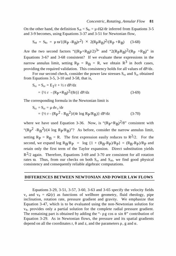
Concentric, Rotating, Annular Flow 81
On the other hand, the definition Srθ = Sθr = µ dΩ/dr inferred from Equations 3-5and 3-9 becomes, using Equations 3-37 and 3-51 for Newtonian flow,
Srθ = Sθr = µ ω/(RP -RB)r2 × 2(RPRB)2/(RP +RB) (3-68)
Are the two second factors “((RP+RB)/2)3” and “2(RPRB)2/(RP +RB)” in
Equations 3-67 and 3-68 consistent? If we evaluate these expressions in the
narrow annulus limit, setting RP = RB = R, we obtain R3 in both cases,
providing the required validation. This consistency holds for all values of dP/dz.For our second check, consider the power law stresses Srz and Szr obtained
from Equations 3-5, 3-10 and 3-58, that is,
Srz = Szr = E1/r + ½ r dP/dz
= ½ r - (RP+RB)2/(8r) dP/dz (3-69)
The corresponding formula in the Newtonian limit is
Srz = Szr = µ dvz /dr
= ½ r - (RP2 - RB
2)/(4r log RP/RB) dP/dz (3-70)
where we have used Equation 3-36. Now, is “(RP+RB)2/8” consistent with
“(RP2 -RB
2)/(4 log RP/RB)”? As before, consider the narrow annulus limit,
setting RP = RB = R. The first expression easily reduces to R2/2. For the
second, we expand log RB/RP = log 1 + (RB-RP)/RP = (RB-RP)/RP and
retain only the first term of the Taylor expansion. Direct substitution yields
R2/2 again. Therefore, Equations 3-69 and 3-70 are consistent for all rotationrates ω. Thus, from our checks on both Srz and Srθ, we find good physicalconsistency and consequently reliable algebraic computations.
DIFFERENCES BETWEEN NEWTONIAN AND POWER LAW FLOWS
Equations 3-29, 3-51, 3-57, 3-60, 3-63 and 3-65 specify the velocity fieldsvz and vθ = rΩ(r) as functions of wellbore geometry, fluid rheology, pipeinclination, rotation rate, pressure gradient and gravity. We emphasize thatEquation 3-47, which is to be evaluated using the non-Newtonian solution forvθ, provides only a partial solution for the complete radial pressure gradient.The remaining part is obtained by adding the “- ρg cos α sin θ” contribution ofEquation 3-29. As in Newtonian flows, the pressure and its spatial gradientsdepend on all the coordinates r, θ and z, and the parameters ρ, g and α.
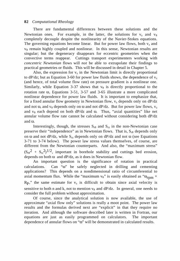
82 Computational Rheology
There are fundamental differences between these solutions and theNewtonian ones. For example, in the latter, the solutions for vz and vθcompletely decouple despite the nonlinearity of the Navier-Stokes equations.The governing equations become linear. But for power law flows, both vz andvθ remain highly coupled and nonlinear. In this sense, Newtonian results aresingular; but the degeneracy disappears for eccentric geometries when theconvective terms reappear. Cuttings transport experimenters working withconcentric Newtonian flows will not be able to extrapolate their findings topractical geometries or fluids. This will be discussed in detail in Chapter 5.
Also, the expression for vz in the Newtonian limit is directly proportionalto dP/dz; but as Equation 3-60 for power law fluids shows, the dependence of vz
(and hence, of total volume flow rate) on pressure gradient is a nonlinear one.Similarly, while Equation 3-37 shows that vθ is directly proportional to therotation rate ω, Equations 3-51, 3-57 and 3-65 illustrate a more complicatednonlinear dependence for power law fluids. It is important to emphasize that,for a fixed annular flow geometry in Newtonian flow, vz depends only on dP/dzand not ω, and vθ depends only on ω and not dP/dz. But for power law flows, vz
and vθ each depend on both dP/dz and ω. Thus, “axial quantities” like netannular volume flow rate cannot be calculated without considering both dP/dzand ω.
Interestingly, though, the stresses Srθ and Srz in the non-Newtonian casepreserve their “independence” as in Newtonian flows. That is, Srθ depends onlyon ω and not dP/dz, while Srz depends only on dP/dz and not ω (see Equations3-71 to 3-74 below). The power law stress values themselves, of course, aredifferent from the Newtonian counterparts. And also, the “maximum stress”
(Srθ2 + Srz
2)1/2, important in borehole stability and cuttings bed erosion,depends on both ω and dP/dz, as it does in Newtonian flow.
An important question is the significance of rotation in practicalcalculations. Can “ω” be safely neglected in drilling and cementingapplications? This depends on a nondimensional ratio of circumferential toaxial momentum flux. While the “maximum vθ” is easily obtained as “ωrpm ×RP,” the same estimate for vz is difficult to obtain since axial velocity is
sensitive to both n and k, not to mention vθ and dP/dz. In general, one needs toconsider the full problem without approximation.
Of course, since the analytical solution is now available, the use ofapproximate “axial flow only” solutions is really a moot point. The power lawresults and the formulas derived next are “explicit” in that they require noiteration. And although the software described later is written in Fortran, ourequations are just as easily programmed on calculators. The importantdependence of annular flows on “ω” will be demonstrated in calculated results.
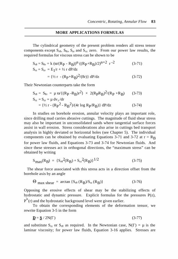
Concentric, Rotating, Annular Flow 83
MORE APPLICATIONS FORMULAS
The cylindrical geometry of the present problem renders all stress tensorcomponents except Srθ, Sθr, Szr and Srz zero. From our power law results, therequired formulas for viscous stress can be shown to be
Srθ = Sθr = k (ω/(RP - RB))n ((RP+RB)/2)n+2 r -2 (3-71)
Srz = Szr = E1/r + ½ r dP/dz
= ½ r - (RP+RB)2/(8r) dP/dz (3-72)
Their Newtonian counterparts take the form
Srθ = Sθr = µ ω/(RP -RB)r2 × 2(RPRB)2/(RP +RB) (3-73)
Srz = Szr = µ dvz /dr
= ½ r - (RP2 - RB
2)/(4r log RP/RB) dP/dz (3-74)
In studies on borehole erosion, annular velocity plays an important role,since drilling mud carries abrasive cuttings. The magnitude of fluid shear stressmay also be important in unconsolidated sands where tangential surface forcesassist in wall erosion. Stress considerations also arise in cuttings bed transportanalysis in highly deviated or horizontal holes (see Chapter 5). The individualcomponents can be obtained by evaluating Equations 3-71 and 3-72 at r = RBfor power law fluids, and Equations 3-73 and 3-74 for Newtonian fluids. Andsince these stresses act in orthogonal directions, the “maximum stress” can beobtained by writing
Smax(RB) = Srθ2(RB) + Srz
2(RB)1/2 (3-75)
The shear force associated with this stress acts in a direction offset from theborehole axis by an angle
Θ max shear = arctan Srθ (RB)/Srz (RB) (3-76)
Opposing the erosive effects of shear may be the stabilizing effects ofhydrostatic and dynamic pressure. Explicit formulas for the pressures P(z),
P*(r) and the hydrostatic background level were given earlier.To obtain the corresponding elements of the deformation tensor, we
rewrite Equation 3-5 in the form
D = S / 2N(Γ) (3-77)
and substitute Srz or Srθ as required. In the Newtonian case, N(Γ) = µ is thelaminar viscosity; for power law fluids, Equation 3-16 applies. Stresses are
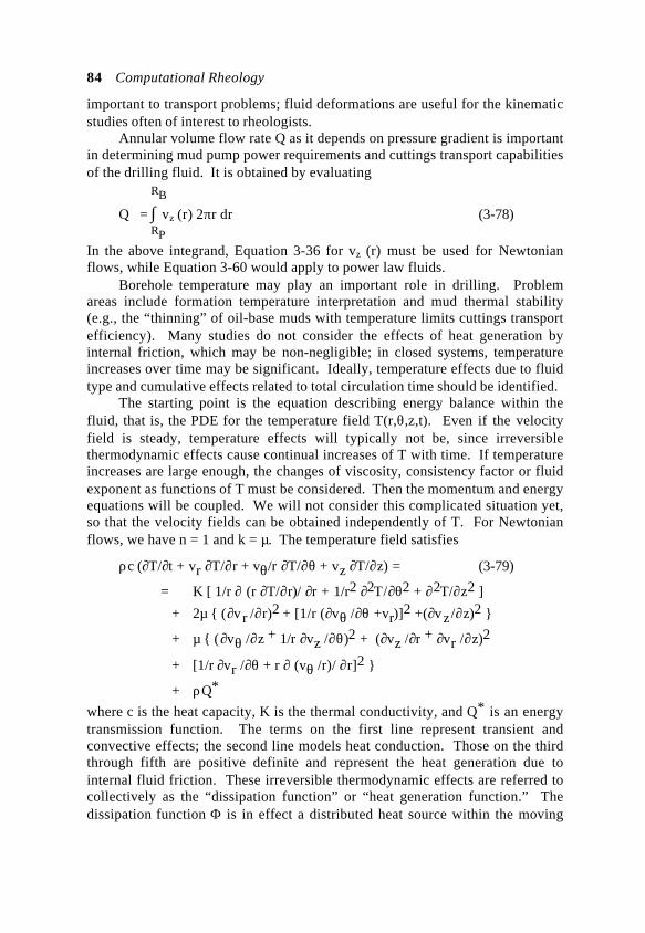
84 Computational Rheology
important to transport problems; fluid deformations are useful for the kinematicstudies often of interest to rheologists.
Annular volume flow rate Q as it depends on pressure gradient is importantin determining mud pump power requirements and cuttings transport capabilitiesof the drilling fluid. It is obtained by evaluating RB
Q = ∫ vz (r) 2πr dr (3-78) RPIn the above integrand, Equation 3-36 for vz (r) must be used for Newtonianflows, while Equation 3-60 would apply to power law fluids.
Borehole temperature may play an important role in drilling. Problemareas include formation temperature interpretation and mud thermal stability(e.g., the “thinning” of oil-base muds with temperature limits cuttings transportefficiency). Many studies do not consider the effects of heat generation byinternal friction, which may be non-negligible; in closed systems, temperatureincreases over time may be significant. Ideally, temperature effects due to fluidtype and cumulative effects related to total circulation time should be identified.
The starting point is the equation describing energy balance within thefluid, that is, the PDE for the temperature field T(r,θ,z,t). Even if the velocityfield is steady, temperature effects will typically not be, since irreversiblethermodynamic effects cause continual increases of T with time. If temperatureincreases are large enough, the changes of viscosity, consistency factor or fluidexponent as functions of T must be considered. Then the momentum and energyequations will be coupled. We will not consider this complicated situation yet,so that the velocity fields can be obtained independently of T. For Newtonianflows, we have n = 1 and k = µ. The temperature field satisfies
ρc (∂T/∂t + vr ∂T/∂r + vθ/r ∂T/∂θ + vz ∂T/∂z) = (3-79)
= K [ 1/r ∂ (r ∂T/∂r)/ ∂r + 1/r2 ∂2T/∂θ2 + ∂2T/∂z2 ]
+ 2µ (∂vr /∂r)2 + [1/r (∂vθ /∂θ +vr)]2 +(∂vz /∂z)2
+ µ (∂vθ /∂z + 1/r ∂vz /∂θ)2 + (∂vz /∂r + ∂vr /∂z)2
+ [1/r ∂vr /∂θ + r ∂ (vθ /r)/ ∂r]2
+ ρQ*
where c is the heat capacity, K is the thermal conductivity, and Q* is an energytransmission function. The terms on the first line represent transient andconvective effects; the second line models heat conduction. Those on the thirdthrough fifth are positive definite and represent the heat generation due tointernal fluid friction. These irreversible thermodynamic effects are referred tocollectively as the “dissipation function” or “heat generation function.” Thedissipation function Φ is in effect a distributed heat source within the moving
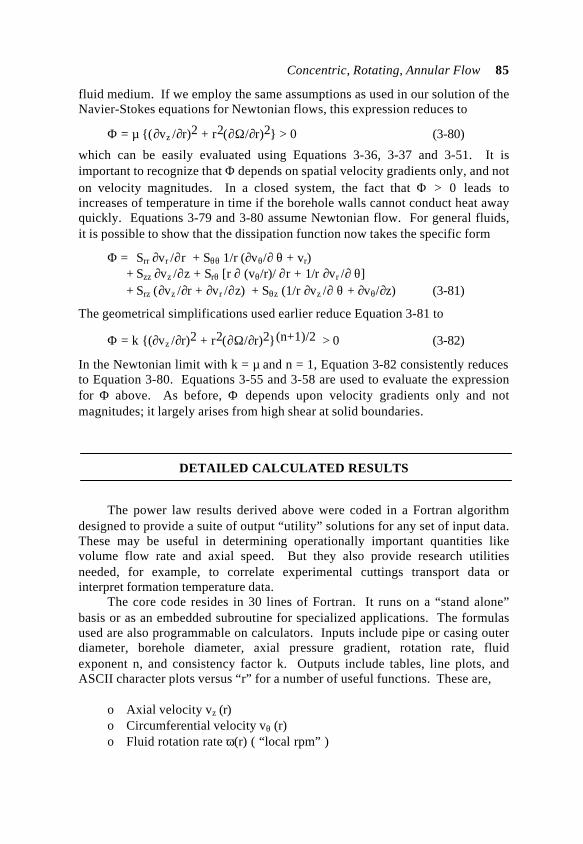
Concentric, Rotating, Annular Flow 85
fluid medium. If we employ the same assumptions as used in our solution of theNavier-Stokes equations for Newtonian flows, this expression reduces to
Φ = µ (∂vz /∂r)2 + r2(∂Ω/∂r)2 > 0 (3-80)
which can be easily evaluated using Equations 3-36, 3-37 and 3-51. It isimportant to recognize that Φ depends on spatial velocity gradients only, and noton velocity magnitudes. In a closed system, the fact that Φ > 0 leads toincreases of temperature in time if the borehole walls cannot conduct heat awayquickly. Equations 3-79 and 3-80 assume Newtonian flow. For general fluids,it is possible to show that the dissipation function now takes the specific form
Φ = Srr ∂vr /∂r + Sθθ 1/r (∂vθ/∂ θ + vr) + Szz ∂vz /∂z + Srθ [r ∂ (vθ/r)/ ∂r + 1/r ∂vr /∂ θ] + Srz (∂vz /∂r + ∂vr /∂z) + Sθz (1/r ∂vz /∂ θ + ∂vθ/∂z) (3-81)
The geometrical simplifications used earlier reduce Equation 3-81 to
Φ = k (∂vz /∂r)2 + r2(∂Ω/∂r)2(n+1)/2 > 0 (3-82)
In the Newtonian limit with k = µ and n = 1, Equation 3-82 consistently reducesto Equation 3-80. Equations 3-55 and 3-58 are used to evaluate the expressionfor Φ above. As before, Φ depends upon velocity gradients only and notmagnitudes; it largely arises from high shear at solid boundaries.
DETAILED CALCULATED RESULTS
The power law results derived above were coded in a Fortran algorithmdesigned to provide a suite of output “utility” solutions for any set of input data.These may be useful in determining operationally important quantities likevolume flow rate and axial speed. But they also provide research utilitiesneeded, for example, to correlate experimental cuttings transport data orinterpret formation temperature data.
The core code resides in 30 lines of Fortran. It runs on a “stand alone”basis or as an embedded subroutine for specialized applications. The formulasused are also programmable on calculators. Inputs include pipe or casing outerdiameter, borehole diameter, axial pressure gradient, rotation rate, fluidexponent n, and consistency factor k. Outputs include tables, line plots, andASCII character plots versus “r” for a number of useful functions. These are,
o Axial velocity vz (r)o Circumferential velocity vθ (r)o Fluid rotation rate ω(r) ( “local rpm” )
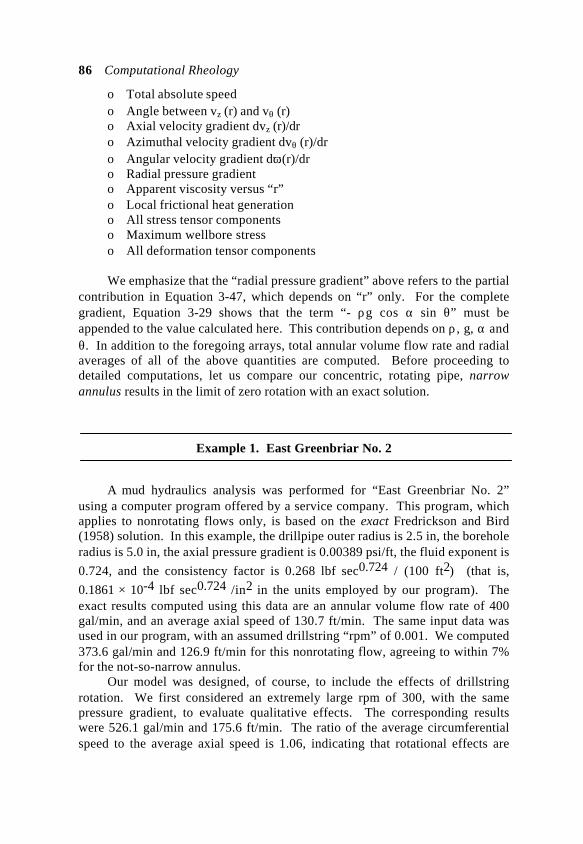
86 Computational Rheology
o Total absolute speedo Angle between vz (r) and vθ (r)o Axial velocity gradient dvz (r)/dro Azimuthal velocity gradient dvθ (r)/dro Angular velocity gradient dω(r)/dro Radial pressure gradiento Apparent viscosity versus “r”o Local frictional heat generationo All stress tensor componentso Maximum wellbore stresso All deformation tensor components
We emphasize that the “radial pressure gradient” above refers to the partialcontribution in Equation 3-47, which depends on “r” only. For the completegradient, Equation 3-29 shows that the term “- ρg cos α sin θ” must beappended to the value calculated here. This contribution depends on ρ, g, α andθ. In addition to the foregoing arrays, total annular volume flow rate and radialaverages of all of the above quantities are computed. Before proceeding todetailed computations, let us compare our concentric, rotating pipe, narrowannulus results in the limit of zero rotation with an exact solution.
Example 1. East Greenbriar No. 2
A mud hydraulics analysis was performed for “East Greenbriar No. 2”using a computer program offered by a service company. This program, whichapplies to nonrotating flows only, is based on the exact Fredrickson and Bird(1958) solution. In this example, the drillpipe outer radius is 2.5 in, the boreholeradius is 5.0 in, the axial pressure gradient is 0.00389 psi/ft, the fluid exponent is
0.724, and the consistency factor is 0.268 lbf sec0.724 / (100 ft2) (that is,
0.1861 × 10⁻⁴ lbf sec0.724 /in2 in the units employed by our program). Theexact results computed using this data are an annular volume flow rate of 400gal/min, and an average axial speed of 130.7 ft/min. The same input data wasused in our program, with an assumed drillstring “rpm” of 0.001. We computed373.6 gal/min and 126.9 ft/min for this nonrotating flow, agreeing to within 7%for the not-so-narrow annulus.
Our model was designed, of course, to include the effects of drillstringrotation. We first considered an extremely large rpm of 300, with the samepressure gradient, to evaluate qualitative effects. The corresponding resultswere 526.1 gal/min and 175.6 ft/min. The ratio of the average circumferentialspeed to the average axial speed is 1.06, indicating that rotational effects are
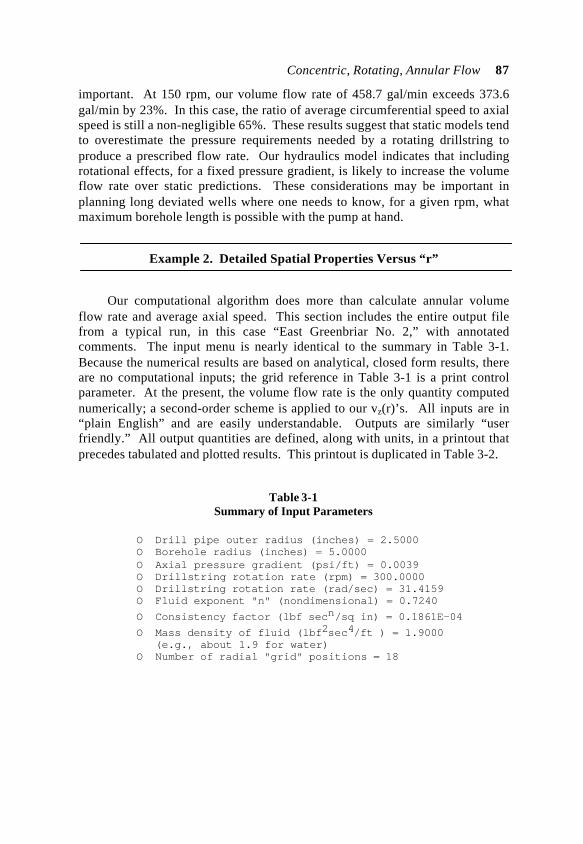
Concentric, Rotating, Annular Flow 87
important. At 150 rpm, our volume flow rate of 458.7 gal/min exceeds 373.6gal/min by 23%. In this case, the ratio of average circumferential speed to axialspeed is still a non-negligible 65%. These results suggest that static models tendto overestimate the pressure requirements needed by a rotating drillstring toproduce a prescribed flow rate. Our hydraulics model indicates that includingrotational effects, for a fixed pressure gradient, is likely to increase the volumeflow rate over static predictions. These considerations may be important inplanning long deviated wells where one needs to know, for a given rpm, whatmaximum borehole length is possible with the pump at hand.
Example 2. Detailed Spatial Properties Versus “r”
Our computational algorithm does more than calculate annular volumeflow rate and average axial speed. This section includes the entire output filefrom a typical run, in this case “East Greenbriar No. 2,” with annotatedcomments. The input menu is nearly identical to the summary in Table 3-1.Because the numerical results are based on analytical, closed form results, thereare no computational inputs; the grid reference in Table 3-1 is a print controlparameter. At the present, the volume flow rate is the only quantity computednumerically; a second-order scheme is applied to our vz(r)’s. All inputs are in“plain English” and are easily understandable. Outputs are similarly “userfriendly.” All output quantities are defined, along with units, in a printout thatprecedes tabulated and plotted results. This printout is duplicated in Table 3-2.
Table 3-1Summary of Input Parameters
O Drill pipe outer radius (inches) = 2.5000O Borehole radius (inches) = 5.0000O Axial pressure gradient (psi/ft) = 0.0039O Drillstring rotation rate (rpm) = 300.0000O Drillstring rotation rate (rad/sec) = 31.4159O Fluid exponent "n" (nondimensional) = 0.7240
O Consistency factor (lbf secn/sq in) = 0.1861E-04
O Mass density of fluid (lbf2sec4/ft ) = 1.9000 (e.g., about 1.9 for water)
O Number of radial "grid" positions = 18
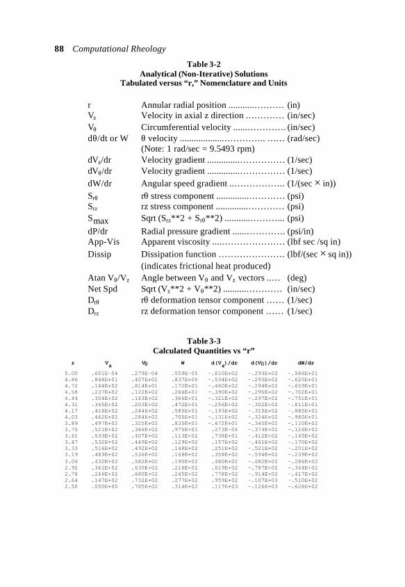
88 Computational Rheology
Table 3-2Analytical (Non-Iterative) Solutions
Tabulated versus “r,” Nomenclature and Units
r Annular radial position ...........………. (in)Vz Velocity in axial z direction .………… (in/sec)Vθ Circumferential velocity ......…………. (in/sec)dθ/dt or W θ velocity ...................………….. …… (rad/sec) (Note: 1 rad/sec = 9.5493 rpm)dVz/dr Velocity gradient ..............…………… (1/sec)dVθ/dr Velocity gradient ..............…………… (1/sec)dW/dr Angular speed gradient ..…………….. (1/(sec × in))Srθ rθ stress component ..............………… (psi)Srz rz stress component ..............………… (psi)Smax Sqrt (Srz**2 + Srθ**2) ...........………... (psi)
dP/dr Radial pressure gradient ......…………. (psi/in)App-Vis Apparent viscosity ....………………… (lbf sec /sq in)Dissip Dissipation function …………………. (lbf/(sec × sq in)) (indicates frictional heat produced)Atan Vθ/Vz Angle between Vθ and Vz vectors ..… (deg)Net Spd Sqrt (Vz**2 + Vθ**2) ..........………… (in/sec)Drθ rθ deformation tensor component …… (1/sec)Drz rz deformation tensor component …… (1/sec)
Table 3-3Calculated Quantities vs “r”
r Vz Vθ W d(Vz)/dr d(Vθ)/dr dW/dr
5.00 .601E-04 .279E-04 .559E-05 -.610E+02 -.293E+02 -.586E+01 4.86 .848E+01 .407E+01 .837E+00 -.534E+02 -.293E+02 -.620E+01 4.72 .164E+02 .814E+01 .172E+01 -.460E+02 -.294E+02 -.659E+01 4.58 .237E+02 .122E+02 .266E+01 -.390E+02 -.295E+02 -.702E+01 4.44 .304E+02 .163E+02 .366E+01 -.321E+02 -.297E+02 -.751E+01 4.31 .365E+02 .203E+02 .472E+01 -.256E+02 -.302E+02 -.811E+01 4.17 .418E+02 .244E+02 .585E+01 -.193E+02 -.310E+02 -.885E+01 4.03 .462E+02 .284E+02 .705E+01 -.131E+02 -.324E+02 -.980E+01 3.89 .497E+02 .325E+02 .835E+01 -.672E+01 -.345E+02 -.110E+02 3.75 .521E+02 .366E+02 .975E+01 .273E-04 -.374E+02 -.126E+02 3.61 .533E+02 .407E+02 .113E+02 .738E+01 -.412E+02 -.145E+02 3.47 .532E+02 .449E+02 .129E+02 .157E+02 -.461E+02 -.170E+02 3.33 .516E+02 .492E+02 .148E+02 .251E+02 -.521E+02 -.201E+02 3.19 .483E+02 .536E+02 .168E+02 .358E+02 -.594E+02 -.239E+02 3.06 .432E+02 .582E+02 .190E+02 .480E+02 -.682E+02 -.286E+02 2.92 .361E+02 .630E+02 .216E+02 .619E+02 -.787E+02 -.344E+02 2.78 .266E+02 .680E+02 .245E+02 .778E+02 -.914E+02 -.417E+02 2.64 .147E+02 .732E+02 .277E+02 .959E+02 -.107E+03 -.510E+02 2.50 .000E+00 .785E+02 .314E+02 .117E+03 -.126E+03 -.628E+02
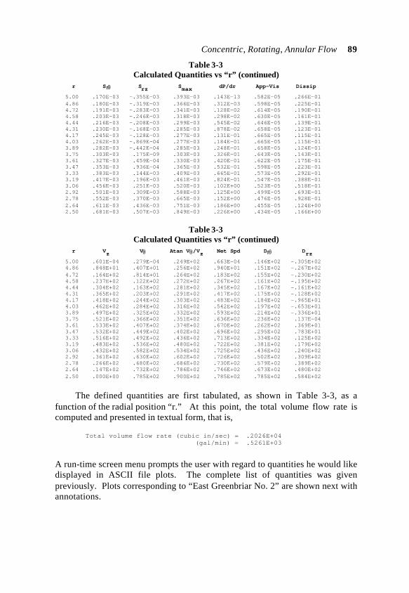
Concentric, Rotating, Annular Flow 89
Table 3-3Calculated Quantities vs “r” (continued)
r Srθ Srz Smax dP/dr App-Vis Dissip
5.00 .170E-03 -.355E-03 .393E-03 .143E-13 .582E-05 .266E-01 4.86 .180E-03 -.319E-03 .366E-03 .312E-03 .598E-05 .225E-01 4.72 .191E-03 -.283E-03 .341E-03 .128E-02 .614E-05 .190E-01 4.58 .203E-03 -.246E-03 .318E-03 .298E-02 .630E-05 .161E-01 4.44 .216E-03 -.208E-03 .299E-03 .545E-02 .646E-05 .139E-01 4.31 .230E-03 -.168E-03 .285E-03 .878E-02 .658E-05 .123E-01 4.17 .245E-03 -.128E-03 .277E-03 .131E-01 .665E-05 .115E-01 4.03 .262E-03 -.869E-04 .277E-03 .184E-01 .665E-05 .115E-01 3.89 .282E-03 -.442E-04 .285E-03 .248E-01 .658E-05 .124E-01 3.75 .303E-03 .175E-09 .303E-03 .326E-01 .643E-05 .143E-01 3.61 .327E-03 .459E-04 .330E-03 .420E-01 .622E-05 .175E-01 3.47 .353E-03 .936E-04 .365E-03 .532E-01 .598E-05 .223E-01 3.33 .383E-03 .144E-03 .409E-03 .665E-01 .573E-05 .292E-01 3.19 .417E-03 .196E-03 .461E-03 .824E-01 .547E-05 .388E-01 3.06 .456E-03 .251E-03 .520E-03 .102E+00 .523E-05 .518E-01 2.92 .501E-03 .309E-03 .588E-03 .125E+00 .499E-05 .693E-01 2.78 .552E-03 .370E-03 .665E-03 .152E+00 .476E-05 .928E-01 2.64 .611E-03 .436E-03 .751E-03 .186E+00 .455E-05 .124E+00 2.50 .681E-03 .507E-03 .849E-03 .226E+00 .434E-05 .166E+00
Table 3-3Calculated Quantities vs “r” (continued)
r Vz Vθ Atan Vθ/Vz Net Spd Drθ Drz 5.00 .601E-04 .279E-04 .249E+02 .663E-04 .146E+02 -.305E+02 4.86 .848E+01 .407E+01 .256E+02 .940E+01 .151E+02 -.267E+02 4.72 .164E+02 .814E+01 .264E+02 .183E+02 .155E+02 -.230E+02 4.58 .237E+02 .122E+02 .272E+02 .267E+02 .161E+02 -.195E+02 4.44 .304E+02 .163E+02 .281E+02 .345E+02 .167E+02 -.161E+02 4.31 .365E+02 .203E+02 .291E+02 .417E+02 .175E+02 -.128E+02 4.17 .418E+02 .244E+02 .303E+02 .483E+02 .184E+02 -.965E+01 4.03 .462E+02 .284E+02 .316E+02 .542E+02 .197E+02 -.653E+01 3.89 .497E+02 .325E+02 .332E+02 .593E+02 .214E+02 -.336E+01 3.75 .521E+02 .366E+02 .351E+02 .636E+02 .236E+02 .137E-04 3.61 .533E+02 .407E+02 .374E+02 .670E+02 .262E+02 .369E+01 3.47 .532E+02 .449E+02 .402E+02 .696E+02 .295E+02 .783E+01 3.33 .516E+02 .492E+02 .436E+02 .713E+02 .334E+02 .125E+02 3.19 .483E+02 .536E+02 .480E+02 .722E+02 .381E+02 .179E+02 3.06 .432E+02 .582E+02 .534E+02 .725E+02 .436E+02 .240E+02 2.92 .361E+02 .630E+02 .602E+02 .726E+02 .502E+02 .309E+02 2.78 .266E+02 .680E+02 .686E+02 .730E+02 .579E+02 .389E+02 2.64 .147E+02 .732E+02 .786E+02 .746E+02 .673E+02 .480E+02 2.50 .000E+00 .785E+02 .900E+02 .785E+02 .785E+02 .584E+02
The defined quantities are first tabulated, as shown in Table 3-3, as afunction of the radial position “r.” At this point, the total volume flow rate iscomputed and presented in textual form, that is,
Total volume flow rate (cubic in/sec) = .2026E+04 (gal/min) = .5261E+03
A run-time screen menu prompts the user with regard to quantities he would likedisplayed in ASCII file plots. The complete list of quantities was givenpreviously. Plots corresponding to “East Greenbriar No. 2” are shown next withannotations.
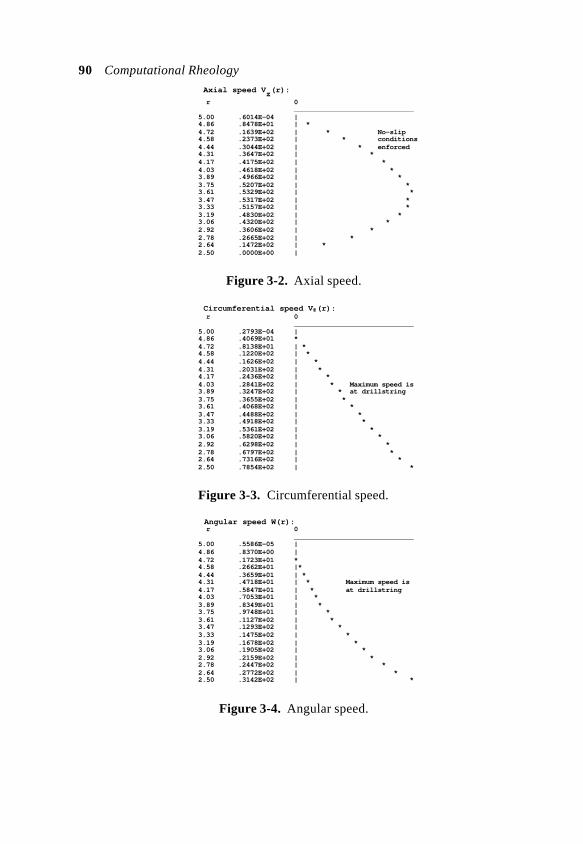
90 Computational Rheology
Axial speed Vz(r):
r 0 ______________________________ 5.00 .6014E-04 | 4.86 .8478E+01 | * 4.72 .1639E+02 | * No-slip 4.58 .2373E+02 | * conditions 4.44 .3044E+02 | * enforced 4.31 .3647E+02 | * 4.17 .4175E+02 | * 4.03 .4618E+02 | * 3.89 .4966E+02 | * 3.75 .5207E+02 | * 3.61 .5329E+02 | * 3.47 .5317E+02 | * 3.33 .5157E+02 | * 3.19 .4830E+02 | * 3.06 .4320E+02 | * 2.92 .3606E+02 | * 2.78 .2665E+02 | * 2.64 .1472E+02 | * 2.50 .0000E+00 |
Figure 3-2. Axial speed.
Circumferential speed V θθ(r): r 0 ______________________________ 5.00 .2793E-04 | 4.86 .4069E+01 * 4.72 .8138E+01 | * 4.58 .1220E+02 | * 4.44 .1626E+02 | * 4.31 .2031E+02 | * 4.17 .2436E+02 | * 4.03 .2841E+02 | * Maximum speed is 3.89 .3247E+02 | * at drillstring 3.75 .3655E+02 | * 3.61 .4068E+02 | * 3.47 .4488E+02 | * 3.33 .4918E+02 | * 3.19 .5361E+02 | * 3.06 .5820E+02 | * 2.92 .6298E+02 | * 2.78 .6797E+02 | * 2.64 .7316E+02 | * 2.50 .7854E+02 | *
Figure 3-3. Circumferential speed.
Angular speed W(r): r 0 ______________________________ 5.00 .5586E-05 | 4.86 .8370E+00 | 4.72 .1723E+01 * 4.58 .2662E+01 |* 4.44 .3659E+01 | * 4.31 .4718E+01 | * Maximum speed is 4.17 .5847E+01 | * at drillstring 4.03 .7053E+01 | * 3.89 .8349E+01 | * 3.75 .9748E+01 | * 3.61 .1127E+02 | * 3.47 .1293E+02 | * 3.33 .1475E+02 | * 3.19 .1678E+02 | * 3.06 .1905E+02 | * 2.92 .2159E+02 | * 2.78 .2447E+02 | * 2.64 .2772E+02 | * 2.50 .3142E+02 | *
Figure 3-4. Angular speed.
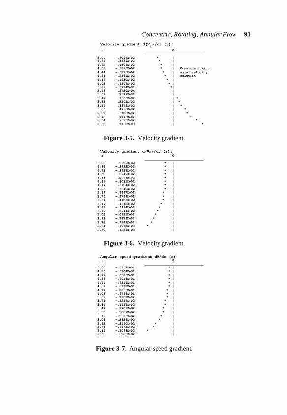
Concentric, Rotating, Annular Flow 91 Velocity gradient d(Vz)/dr (r):
r 0 ______________________________ 5.00 -.6096E+02 * | 4.86 -.5339E+02 * | 4.72 -.4604E+02 * | 4.58 -.3896E+02 * | Consistent with 4.44 -.3215E+02 * | axial velocity 4.31 -.2561E+02 * | solution 4.17 -.1930E+02 * | 4.03 -.1307E+02 * | 3.89 -.6724E+01 *| 3.75 .2730E-04 | 3.61 .7377E+01 | 3.47 .1566E+02 | * 3.33 .2505E+02 | * 3.19 .3575E+02 | * 3.06 .4796E+02 | * 2.92 .6188E+02 | * 2.78 .7776E+02 | * 2.64 .9593E+02 | * 2.50 .1168E+03 | *
Figure 3-5. Velocity gradient.
Velocity gradient d(V θθ)/dr (r): r 0 ______________________________ 5.00 -.2929E+02 * | 4.86 -.2932E+02 * | 4.72 -.2938E+02 * | 4.58 -.2949E+02 * | 4.44 -.2974E+02 * | 4.31 -.3021E+02 * | 4.17 -.3104E+02 * | 4.03 -.3240E+02 * | 3.89 -.3447E+02 * | 3.75 -.3738E+02 * | 3.61 -.4123E+02 * | 3.47 -.4612E+02 * | 3.33 -.5214E+02 * | 3.19 -.5944E+02 * | 3.06 -.6821E+02 * | 2.92 -.7874E+02 * | 2.78 -.9142E+02 * | 2.64 -.1068E+03 * | 2.50 -.1257E+03 |
Figure 3-6. Velocity gradient.
Angular speed gradient dW/dr (r): r 0 ______________________________ 5.00 -.5857E+01 * | 4.86 -.6204E+01 * | 4.72 -.6586E+01 * | 4.58 -.7016E+01 * | 4.44 -.7514E+01 * | 4.31 -.8112E+01 * | 4.17 -.8853E+01 * | 4.03 -.9796E+01 * | 3.89 -.1101E+02 * | 3.75 -.1257E+02 * | 3.61 -.1454E+02 * | 3.47 -.1701E+02 * | 3.33 -.2007E+02 * | 3.19 -.2386E+02 * | 3.06 -.2856E+02 * | 2.92 -.3440E+02 * | 2.78 -.4172E+02 * | 2.64 -.5098E+02 * | 2.50 -.6283E+02 |
Figure 3-7. Angular speed gradient.
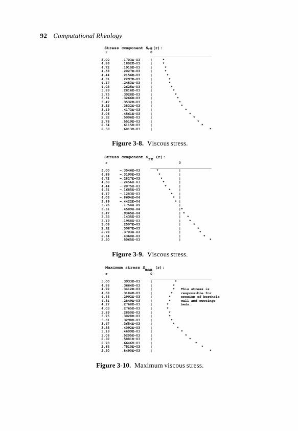
92 Computational Rheology
Stress component Sr θθ(r): r 0 ______________________________ 5.00 .1703E-03 | * 4.86 .1802E-03 | * 4.72 .1910E-03 | * 4.58 .2027E-03 | * 4.44 .2156E-03 | * 4.31 .2297E-03 | * 4.17 .2453E-03 | * 4.03 .2625E-03 | * 3.89 .2816E-03 | * 3.75 .3028E-03 | * 3.61 .3266E-03 | * 3.47 .3532E-03 | * 3.33 .3832E-03 | * 3.19 .4173E-03 | * 3.06 .4561E-03 | * 2.92 .5006E-03 | * 2.78 .5519E-03 | * 2.64 .6115E-03 | * 2.50 .6813E-03 | *
Figure 3-8. Viscous stress.
Stress component Srz (r):
r 0 ______________________________ 5.00 -.3546E-03 * | 4.86 -.3190E-03 * | 4.72 -.2827E-03 * | 4.58 -.2456E-03 * | 4.44 -.2075E-03 * | 4.31 -.1685E-03 * | 4.17 -.1283E-03 * | 4.03 -.8694E-04 * | 3.89 -.4422E-04 * | 3.75 .1754E-09 | 3.61 .4589E-04 |* 3.47 .9365E-04 | * 3.33 .1435E-03 | * 3.19 .1958E-03 | * 3.06 .2507E-03 | * 2.92 .3087E-03 | * 2.78 .3703E-03 | * 2.64 .4360E-03 | * 2.50 .5065E-03 | *
Figure 3-9. Viscous stress.
Maximum stress Smax (r):
r 0 ______________________________ 5.00 .3933E-03 | * 4.86 .3664E-03 | * 4.72 .3412E-03 | * This stress is 4.58 .3184E-03 | * responsible for 4.44 .2992E-03 | * erosion of borehole 4.31 .2849E-03 | * wall and cuttings 4.17 .2768E-03 | * beds. 4.03 .2765E-03 | * 3.89 .2850E-03 | * 3.75 .3028E-03 | * 3.61 .3298E-03 | * 3.47 .3654E-03 | * 3.33 .4092E-03 | * 3.19 .4609E-03 | * 3.06 .5205E-03 | * 2.92 .5881E-03 | * 2.78 .6646E-03 | * 2.64 .7510E-03 | * 2.50 .8490E-03 | *
Figure 3-10. Maximum viscous stress.
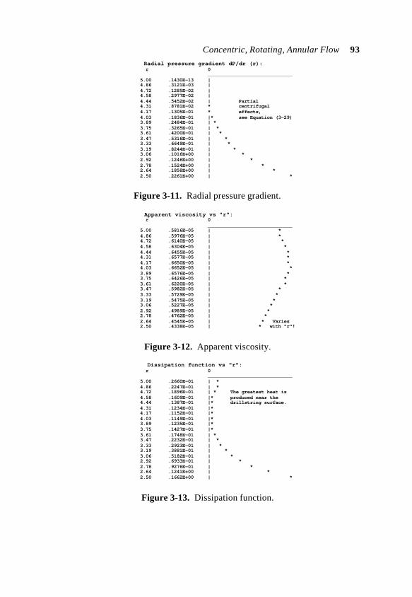
Concentric, Rotating, Annular Flow 93 Radial pressure gradient dP/dr (r): r 0 ______________________________ 5.00 .1430E-13 | 4.86 .3121E-03 | 4.72 .1285E-02 | 4.58 .2977E-02 | 4.44 .5452E-02 | Partial 4.31 .8781E-02 * centrifugal 4.17 .1305E-01 * effects, 4.03 .1836E-01 |* see Equation (3-29) 3.89 .2484E-01 | * 3.75 .3265E-01 | * 3.61 .4200E-01 | * 3.47 .5316E-01 | * 3.33 .6649E-01 | * 3.19 .8244E-01 | * 3.06 .1016E+00 | * 2.92 .1246E+00 | * 2.78 .1524E+00 | * 2.64 .1858E+00 | * 2.50 .2261E+00 | *
Figure 3-11. Radial pressure gradient.
Apparent viscosity vs "r": r 0 ______________________________ 5.00 .5816E-05 | * 4.86 .5976E-05 | * 4.72 .6140E-05 | * 4.58 .6304E-05 | * 4.44 .6455E-05 | * 4.31 .6577E-05 | * 4.17 .6650E-05 | * 4.03 .6652E-05 | * 3.89 .6576E-05 | * 3.75 .6426E-05 | * 3.61 .6220E-05 | * 3.47 .5982E-05 | * 3.33 .5729E-05 | * 3.19 .5475E-05 | * 3.06 .5227E-05 | * 2.92 .4989E-05 | * 2.78 .4762E-05 | * 2.64 .4545E-05 | * Varies 2.50 .4338E-05 | * with "r"!
Figure 3-12. Apparent viscosity.
Dissipation function vs "r": r 0 ______________________________ 5.00 .2660E-01 | * 4.86 .2247E-01 | * 4.72 .1896E-01 | * The greatest heat is 4.58 .1609E-01 |* produced near the 4.44 .1387E-01 |* drillstring surface. 4.31 .1234E-01 |* 4.17 .1152E-01 |* 4.03 .1149E-01 |* 3.89 .1235E-01 |* 3.75 .1427E-01 |* 3.61 .1748E-01 | * 3.47 .2232E-01 | * 3.33 .2923E-01 | * 3.19 .3881E-01 | * 3.06 .5182E-01 | * 2.92 .6933E-01 | * 2.78 .9276E-01 | * 2.64 .1241E+00 | * 2.50 .1662E+00 | *
Figure 3-13. Dissipation function.
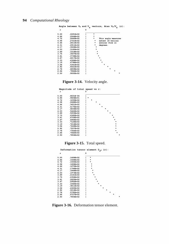
94 Computational Rheology
Angle between V θθ and Vz vectors, Atan V θθ/Vz (r):
r 0 ______________________________ 5.00 .2491E+02 | * 4.86 .2564E+02 | * 4.72 .2640E+02 | * This angle measures 4.58 .2721E+02 | * extent of helical 4.44 .2811E+02 | * annular flow in 4.31 .2911E+02 | * degrees. 4.17 .3026E+02 | * 4.03 .3160E+02 | * 3.89 .3318E+02 | * 3.75 .3507E+02 | * 3.61 .3736E+02 | * 3.47 .4017E+02 | * 3.33 .4364E+02 | * 3.19 .4798E+02 | * 3.06 .5341E+02 | * 2.92 .6021E+02 | * 2.78 .6859E+02 | * 2.64 .7862E+02 | * 2.50 .9000E+02 | *
Figure 3-14. Velocity angle.
Magnitude of total speed vs r: r 0 ______________________________ 5.00 .6631E-04 | 4.86 .9404E+01 | * 4.72 .1830E+02 | * 4.58 .2668E+02 | * 4.44 .3451E+02 | * 4.31 .4175E+02 | * 4.17 .4834E+02 | * 4.03 .5422E+02 | * 3.89 .5933E+02 | * 3.75 .6362E+02 | * 3.61 .6704E+02 | * 3.47 .6958E+02 | * 3.33 .7126E+02 | * 3.19 .7216E+02 | * 3.06 .7249E+02 | * 2.92 .7257E+02 | * 2.78 .7300E+02 | * 2.64 .7462E+02 | * 2.50 .7854E+02 | *
Figure 3-15. Total speed.
Deformation tensor element Drθθ (r):
r 0 ______________________________ 5.00 .1464E+02 | * 4.86 .1508E+02 | * 4.72 .1555E+02 | * 4.58 .1608E+02 | * 4.44 .1670E+02 | * 4.31 .1746E+02 | * 4.17 .1844E+02 | * 4.03 .1973E+02 | * 3.89 .2141E+02 | * 3.75 .2356E+02 | * 3.61 .2625E+02 | * 3.47 .2952E+02 | * 3.33 .3345E+02 | * 3.19 .3811E+02 | * 3.06 .4363E+02 | * 2.92 .5016E+02 | * 2.78 .5795E+02 | * 2.64 .6727E+02 | * 2.50 .7854E+02 | *
Figure 3-16. Deformation tensor element.
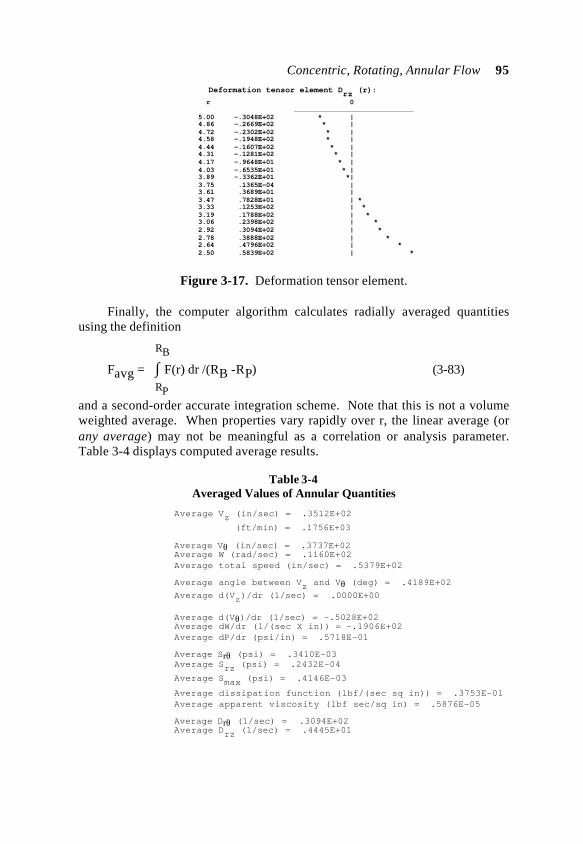
Concentric, Rotating, Annular Flow 95 Deformation tensor element Drz (r):
r 0 ______________________________ 5.00 -.3048E+02 * | 4.86 -.2669E+02 * | 4.72 -.2302E+02 * | 4.58 -.1948E+02 * | 4.44 -.1607E+02 * | 4.31 -.1281E+02 * | 4.17 -.9648E+01 * | 4.03 -.6535E+01 * | 3.89 -.3362E+01 *| 3.75 .1365E-04 | 3.61 .3689E+01 | 3.47 .7828E+01 | * 3.33 .1253E+02 | * 3.19 .1788E+02 | * 3.06 .2398E+02 | * 2.92 .3094E+02 | * 2.78 .3888E+02 | * 2.64 .4796E+02 | * 2.50 .5839E+02 | *
Figure 3-17. Deformation tensor element.
Finally, the computer algorithm calculates radially averaged quantitiesusing the definition
RB
Favg = ∫ F(r) dr /(RB -RP) (3-83)RP
and a second-order accurate integration scheme. Note that this is not a volumeweighted average. When properties vary rapidly over r, the linear average (orany average) may not be meaningful as a correlation or analysis parameter.Table 3-4 displays computed average results.
Table 3-4Averaged Values of Annular Quantities
Average Vz (in/sec) = .3512E+02
(ft/min) = .1756E+03
Average Vθ (in/sec) = .3737E+02Average W (rad/sec) = .1160E+02Average total speed (in/sec) = .5379E+02
Average angle between Vz and Vθ (deg) = .4189E+02Average d(Vz)/dr (1/sec) = .0000E+00
Average d(Vθ)/dr (1/sec) = -.5028E+02Average dW/dr (1/(sec X in)) = -.1906E+02Average dP/dr (psi/in) = .5718E-01
Average Srθ (psi) = .3410E-03Average Srz (psi) = .2432E-04
Average Smax (psi) = .4146E-03
Average dissipation function (lbf/(sec sq in)) = .3753E-01Average apparent viscosity (lbf sec/sq in) = .5876E-05
Average Drθ (1/sec) = .3094E+02Average Drz (1/sec) = .4445E+01
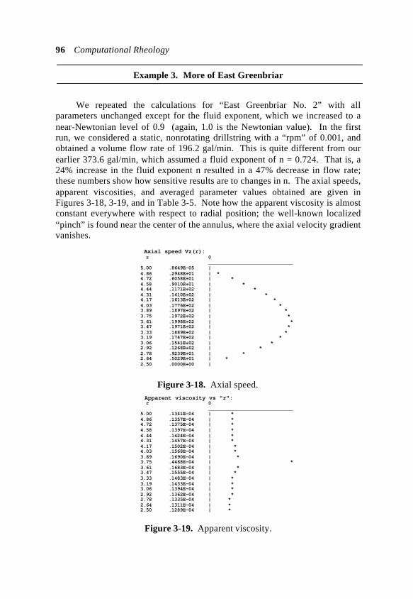
96 Computational Rheology
Example 3. More of East Greenbriar
We repeated the calculations for “East Greenbriar No. 2” with allparameters unchanged except for the fluid exponent, which we increased to anear-Newtonian level of 0.9 (again, 1.0 is the Newtonian value). In the firstrun, we considered a static, nonrotating drillstring with a “rpm” of 0.001, andobtained a volume flow rate of 196.2 gal/min. This is quite different from ourearlier 373.6 gal/min, which assumed a fluid exponent of n = 0.724. That is, a24% increase in the fluid exponent n resulted in a 47% decrease in flow rate;these numbers show how sensitive results are to changes in n. The axial speeds,apparent viscosities, and averaged parameter values obtained are given inFigures 3-18, 3-19, and in Table 3-5. Note how the apparent viscosity is almostconstant everywhere with respect to radial position; the well-known localized“pinch” is found near the center of the annulus, where the axial velocity gradientvanishes.
Axial speed Vz(r): r 0 ______________________________ 5.00 .8649E-05 | 4.86 .2948E+01 | * 4.72 .6058E+01 | * 4.58 .9010E+01 | * 4.44 .1171E+02 | * 4.31 .1410E+02 | * 4.17 .1613E+02 | * 4.03 .1776E+02 | * 3.89 .1897E+02 | * 3.75 .1972E+02 | * 3.61 .1998E+02 | * 3.47 .1971E+02 | * 3.33 .1889E+02 | * 3.19 .1747E+02 | * 3.06 .1541E+02 | * 2.92 .1268E+02 | * 2.78 .9239E+01 | * 2.64 .5029E+01 | * 2.50 .0000E+00 |
Figure 3-18. Axial speed. Apparent viscosity vs "r": r 0 ______________________________ 5.00 .1341E-04 | * 4.86 .1357E-04 | * 4.72 .1375E-04 | * 4.58 .1397E-04 | * 4.44 .1424E-04 | * 4.31 .1457E-04 | * 4.17 .1502E-04 | * 4.03 .1568E-04 | * 3.89 .1690E-04 | * 3.75 .4468E-04 | * 3.61 .1683E-04 | * 3.47 .1555E-04 | * 3.33 .1483E-04 | * 3.19 .1433E-04 | * 3.06 .1394E-04 | * 2.92 .1362E-04 | * 2.78 .1335E-04 | * 2.64 .1311E-04 | * 2.50 .1289E-04 | *
Figure 3-19. Apparent viscosity.
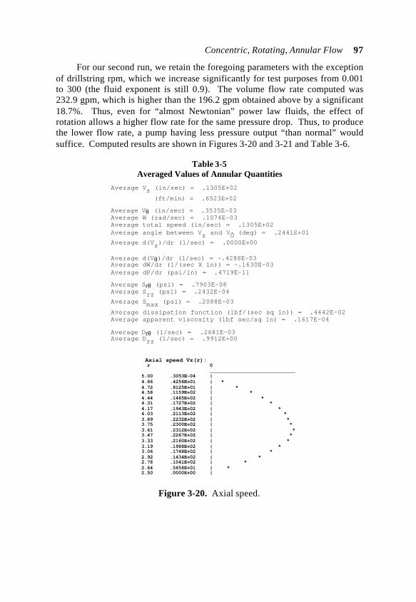
Concentric, Rotating, Annular Flow 97
For our second run, we retain the foregoing parameters with the exceptionof drillstring rpm, which we increase significantly for test purposes from 0.001to 300 (the fluid exponent is still 0.9). The volume flow rate computed was232.9 gpm, which is higher than the 196.2 gpm obtained above by a significant18.7%. Thus, even for “almost Newtonian” power law fluids, the effect ofrotation allows a higher flow rate for the same pressure drop. Thus, to producethe lower flow rate, a pump having less pressure output “than normal” wouldsuffice. Computed results are shown in Figures 3-20 and 3-21 and Table 3-6.
Table 3-5Averaged Values of Annular Quantities
Average Vz (in/sec) = .1305E+02
(ft/min) = .6523E+02
Average Vθ (in/sec) = .3535E-03 Average W (rad/sec) = .1074E-03 Average total speed (in/sec) = .1305E+02 Average angle between Vz and VÕ (deg) = .2441E+01
Average d(Vz)/dr (1/sec) = .0000E+00
Average d(Vθ)/dr (1/sec) = -.4288E-03 Average dW/dr (1/(sec X in)) = -.1630E-03 Average dP/dr (psi/in) = .4719E-11
Average Srθ (psi) = .7903E-08 Average Srz (psi) = .2432E-04
Average Smax (psi) = .2088E-03
Average dissipation function (lbf/(sec sq in)) = .4442E-02 Average apparent viscosity (lbf sec/sq in) = .1617E-04
Average Drθ (1/sec) = .2681E-03 Average Drz (1/sec) = .9912E+00
Axial speed Vz(r): r 0 ______________________________ 5.00 .3053E-04 | 4.86 .4256E+01 | * 4.72 .8125E+01 | * 4.58 .1159E+02 | * 4.44 .1465E+02 | * 4.31 .1727E+02 | * 4.17 .1943E+02 | * 4.03 .2113E+02 | * 3.89 .2232E+02 | * 3.75 .2300E+02 | * 3.61 .2312E+02 | * 3.47 .2267E+02 | * 3.33 .2160E+02 | * 3.19 .1988E+02 | * 3.06 .1748E+02 | * 2.92 .1434E+02 | * 2.78 .1041E+02 | * 2.64 .5656E+01 | * 2.50 .0000E+00 |
Figure 3-20. Axial speed.
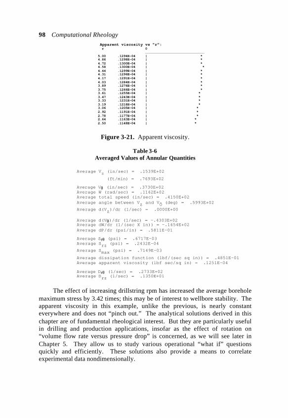
98 Computational Rheology
Apparent viscosity vs "r": r 0 ______________________________ 5.00 .1294E-04 | * 4.86 .1298E-04 | * 4.72 .1300E-04 | * 4.58 .1300E-04 | * 4.44 .1299E-04 | * 4.31 .1296E-04 | * 4.17 .1291E-04 | * 4.03 .1284E-04 | * 3.89 .1276E-04 | * 3.75 .1266E-04 | * 3.61 .1255E-04 | * 3.47 .1243E-04 | * 3.33 .1231E-04 | * 3.19 .1218E-04 | * 3.06 .1205E-04 | * 2.92 .1191E-04 | * 2.78 .1177E-04 | * 2.64 .1163E-04 | * 2.50 .1148E-04 | *
Figure 3-21. Apparent viscosity.
Table 3-6Averaged Values of Annular Quantities
Average Vz (in/sec) = .1539E+02
(ft/min) = .7693E+02
Average Vθ (in/sec) = .3730E+02 Average W (rad/sec) = .1162E+02 Average total speed (in/sec) = .4150E+02 Average angle between Vz and VÕ (deg) = .5993E+02
Average d(Vz)/dr (1/sec) = .0000E+00
Average d(Vθ)/dr (1/sec) = -.4303E+02 Average dW/dr (1/(sec X in)) = -.1654E+02 Average dP/dr (psi/in) = .5811E-01
Average Srθ (psi) = .6717E-03 Average Srz (psi) = .2432E-04
Average Smax (psi) = .7149E-03
Average dissipation function (lbf/(sec sq in)) = .4851E-01 Average apparent viscosity (lbf sec/sq in) = .1251E-04
Average Drθ (1/sec) = .2733E+02 Average Drz (1/sec) = .1350E+01
The effect of increasing drillstring rpm has increased the average boreholemaximum stress by 3.42 times; this may be of interest to wellbore stability. Theapparent viscosity in this example, unlike the previous, is nearly constanteverywhere and does not “pinch out.” The analytical solutions derived in thischapter are of fundamental rheological interest. But they are particularly usefulin drilling and production applications, insofar as the effect of rotation on“volume flow rate versus pressure drop” is concerned, as we will see later inChapter 5. They allow us to study various operational “what if” questionsquickly and efficiently. These solutions also provide a means to correlateexperimental data nondimensionally.
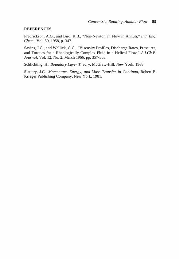
Concentric, Rotating, Annular Flow 99
REFERENCES
Fredrickson, A.G., and Bird, R.B., “Non-Newtonian Flow in Annuli,” Ind. Eng.Chem., Vol. 50, 1958, p. 347.
Savins, J.G., and Wallick, G.C., “Viscosity Profiles, Discharge Rates, Pressures,and Torques for a Rheologically Complex Fluid in a Helical Flow,” A.I.Ch.E.Journal, Vol. 12, No. 2, March 1966, pp. 357-363.
Schlichting, H., Boundary Layer Theory, McGraw-Hill, New York, 1968.
Slattery, J.C., Momentum, Energy, and Mass Transfer in Continua, Robert E.Krieger Publishing Company, New York, 1981.
100
4
Recirculating Annular Vortex Flows
Problems with cuttings accumulation, flow blockage, and resultant stuckpipe in deviated wells are becoming increasingly important operational issues asinterest in horizontal drilling continues. For small angles (ß) from the vertical,annular flows and hole cleaning are well understood; for example, cleaningefficiency is always improved by increasing velocity, viscosity, or both. Butbeyond 30 degrees, these issues are rife with challenging questions. Manyunexplained, confusing, and conflicting observations are reported by differentinvestigators; however, it turns out that bottom viscous stress (which tends toerode cuttings beds having well-defined yield stresses) is the correlationparameter that explains many of these discrepancies.
The next chapter addresses problems related to cuttings transport using theeccentric and rotating flow models developed earlier. Cuttings accumulation, ofcourse, is dangerous because the resulting blockage of the annular spaceincreases the possibility of stuck pipe. Here, we will learn that flows can beblocked even when there is no externally introduced debris in the system. Inother words, dangerous flow blockage can arise from fluid-dynamical effectsalone. This possibility is very real whenever there exist density gradients in adirection perpendicular to the flow, e.g., “barite sag” in the context of drilling.This blockage is also possible in pipe flows of slurries, for instance, slurriescarrying ground wax and hydrate particles or other debris.
In Chapters 2 and 3, the pressure field was assumed to be uniform acrossthe annulus; the velocity field is therefore unidirectional, with the fluid flowingaxially from high pressure regions to low. These assumptions are reasonablesince numerous flows do behave in this manner. In this chapter, we will relaxthese assumptions, but turn to more general flows with density stratification. Aspecial class of annular and pipe flow lends itself to strange occurrences we call“recirculating vortex flows,” to which we now turn our attention.
Recirculating Annular Vortex Flows 101
WHAT ARE RECIRCULATING VORTEX FLOWS?
In deviated holes where circulation has been temporarily interrupted,weighting material such as barite, drilled cuttings or cement additives, may fallout of suspension. Similarly, pipelines containing slurries with wax or hydrateparticles can develop vertical density gradients when flow is temporarily slowedor halted. This gravity stratification has mass density increasing downwards.And this stable stratification, which we collectively refer to as “barite sag,” isthought to be responsible for the trapped, self-contained “recirculation zones” or“bubbles” observed by many experimenters.
They contain rotating, swirling, “ferris-wheel-like” motions within theirinteriors; the external fluid that flows around them “sees” these zones asstationary obstacles that impede their axial movement up the annulus or pipe.Excellent color video tapes showing these vortex-like motions in detail havebeen produced by M-I Drilling Fluids, which were viewed by the author in itsHouston facilities prior to the initial printing of Borehole Flow Modeling.
These strange occurrences are just that; their appearances seem to besporadic and unpredictable, as much myth as reality. However, once they areformed, they remain as stable fluid-dynamical structures that are extremelydifficult to remove. They are dangerous and undesirable because of theirtendency to entrain cuttings, block axial flow, and increase the possibility ofstuck pipe. One might ask, “Why do these bubbles form? What are thecontrolling parameters? How can their occurrences be prevented?”
Detailed study of M-I’s tapes suggests that the recirculating flows formindependently of viscosity and rheology to leading order, that is, they do notdepend primarily on “n” and “k.” They appear to be inertia-dominated,depending on density effects themselves, while nonconservative viscous termsplay only a minor role in sustaining or damping the motion. This leaves thecomponent of density stratification normal to the hole axis as the primaryculprit; it alone is responsible for the highly three-dimensional pressure fieldthat drives local pockets of secondary flow. It is possible, of course, to havemultiple bubbles coexisting along a long deviated hole.
Again these recirculating bubbles, observed near pipe bends, stabilizers,and possibly marine risers and other obstructions, are important for variouspractical reasons. First, they block the streamwise axial flow, resulting in theneed for increased pressure to pass a given volume flow rate. Second, becausethey entrain the mud and further trap drilled cuttings, they are a likely cause ofstuck pipe. Third, the external flow modified by these bubbles can also affectthe very process of cuttings bed formation and removal itself.
Fortunately, these bubbles can be studied, modeled, and characterized in arather simple manner; very instructive “snapshots” of streamline patternscovering a range of vortex effects are given later. This chapter identifies the
102 Computational Rheology
nondimensional channel parameter Ch responsible for vortex bubble formationand describes the physics of these recirculating flows. The equations of motionare given and solved using finite difference methods for several practical flows.The detailed bubble development process is described and illustrated in asequence of computer-generated pictures.
MOTIVATING IDEAS AND CONTROLLING VARIABLES
The governing momentum equations are Euler’s equations, which describelarge-amplitude, inviscid shear flow in both stratified and unstratified media(Schlichting, 1968; Turner, 1973). For the problem at hand, they simplify to
ρuux + vuy = - px (4-1)
ρ uvx + vvy = - py - g ρ cos α (4-2)
ρ ux + ρ vy = 0 (4-3)
We have assumed that the steady vortex flow is contained in a two-dimensional rectangular box in the plane of the hole axis (x) and the direction ofdensity stratification (y). This is based on experimental observation: the vorticalflows do not wrap around the drillpipe. In the above equations, u and v arevelocities in the x and y directions, respectively. Subscripts indicate partialderivatives. Also, ρ is a fluid density that varies linearly with y far upstream,p(x,y) is the unknown pressure field, g is the acceleration due to gravity, and αis the angle the borehole axis makes with the horizontal (α + ß = 90o; also seeChapters 2 and 3). Equations 4-1 and 4-2 are momentum equations in the x andy directions, while Equation 4-3 describes mass conservation.
Nondimensional parameters are important to understanding physicalevents. The well-known Reynolds number, which measures the relative effectsof inertia to viscous forces, is one example of a nondimensional parameter. Italone, for example, dictates the onset of turbulence; also, like Reynolds numbersimply dynamically similar flow patterns. Analogous nondimensional variablesare used in different areas of physics; for instance, the mobility ratio in reservoirengineering or the Mach number in high-speed aerodynamics.
Close examination of Equations 4-1 to 4-3 using affine transformationsshows that the physics of bubble formation depends on a single nondimensionalvariable Ch characterizing the channel flow. It is constructed from the
combination of two simpler ones. The first is a Froude number U2/gL cos α,where U is the average oncoming speed and L is the channel height between thepipe and borehole walls. The second is a relative measure of stratification, saydρ/ρref (dρ might represent the density difference between the bottom and top of
the annulus or pipe, and ρref may be taken as their arithmetic average). The
combined parameter Ch of practical significance is
Recirculating Annular Vortex Flows 103
Ch = U2 ρ ref /gL dρ cos α (4-4)
We now summarize our findings. For large values of Ch, recirculationbubbles will not form; the streamlines of motion are essentially straight and therheology-dominated models developed in Chapters 2 and 3 apply. For smallCh’s of order unity, small recirculation zones do form, and elongate in thestreamwise dimension as Ch decreases. For still smaller values, that is, valuesbelow a critical value of 0.3183, solutions with wavy upstream flows are found,which may or may not be physically realistic.
Equations 4-1 to 4-3 can be solved using “brute force” computationalmethods, but they are more cleverly treated by introducing the streamfunctionused by aerodynamicists and reservoir engineers. When the problem isreformulated in this manner, the result is a nonlinear Poisson equation that canbe easily integrated using fast iterative solvers. Streamlines are obtained byconnecting computed streamfunction elevations having like values. Thearithmetic difference in streamfunction between any two points is directlyproportional to the volume flow rate passing through the two points. Velocityand pressure fields can be obtained by post-processing the computedstreamfunction solutions computed.
DETAILED CALCULATED RESULTS
Typically, the solution obtained for a 20×40 mesh will require less thanone second on Pentium machines. In Figures 4-1 to 4-6, we have allowed theflow to “disappear” into a “mathematical sink” (in practice, the distance to thisobstacle over the height L will appear as a second ratio). This sink simulates thepresence of obstacles or pipe elbows located further upstream. With decreasingvalues of Ch, the appearance of an elongating recirculation bubble is seen. Thecomputed streamline patterns, again constructed by drawing level contours,depict an ever-worsening flowfield. Each figure displays “raw” streamfunctiondata as well as processed contour plots.
The stand-alone vortexes so obtained are inherently stable, since theyrepresent patches of angular momentum that physical laws insist must beconserved. In this sense, they are not unlike isolated trailing aircraft tip vortices,that persist indefinitely in the air until dissipation renders them harmless.However, annular bubbles are worse: the channel flow itself is what drives them,perpetuates them, and increases their ability to do harm by further entrainingsolid debris in the annulus. In the pipeline context, slurry density gradientslikewise promote flow blockage and vortex recirculation; the resulting“sandpapering,” allowing continuous rubbing against pipe walls, can lead tometal erosion, decreased strength, and unexpected rupture.
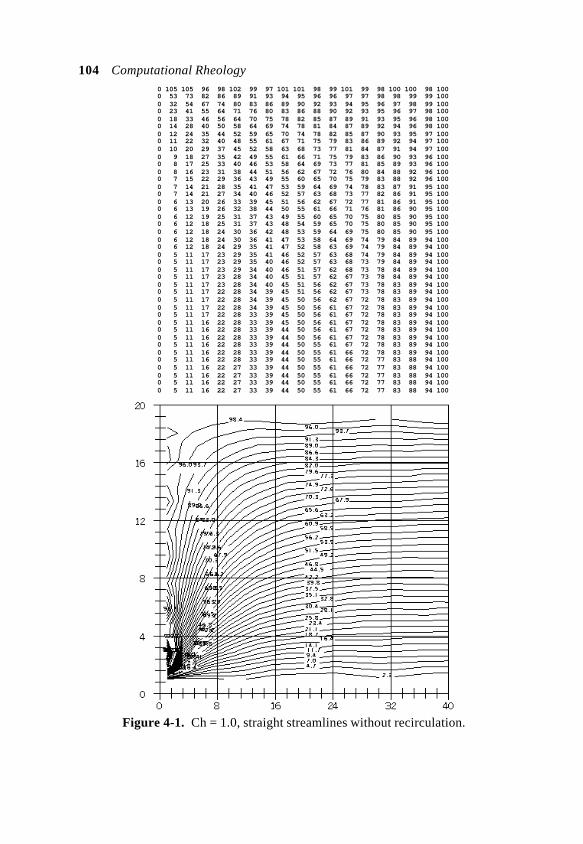
104 Computational Rheology0 105 105 96 98 102 99 97 101 101 98 99 101 99 98 100 100 98 1000 53 73 82 86 89 91 93 94 95 96 96 97 97 98 98 99 99 1000 32 54 67 74 80 83 86 89 90 92 93 94 95 96 97 98 99 1000 23 41 55 64 71 76 80 83 86 88 90 92 93 95 96 97 98 1000 18 33 46 56 64 70 75 78 82 85 87 89 91 93 95 96 98 1000 14 28 40 50 58 64 69 74 78 81 84 87 89 92 94 96 98 1000 12 24 35 44 52 59 65 70 74 78 82 85 87 90 93 95 97 1000 11 22 32 40 48 55 61 67 71 75 79 83 86 89 92 94 97 1000 10 20 29 37 45 52 58 63 68 73 77 81 84 87 91 94 97 1000 9 18 27 35 42 49 55 61 66 71 75 79 83 86 90 93 96 1000 8 17 25 33 40 46 53 58 64 69 73 77 81 85 89 93 96 1000 8 16 23 31 38 44 51 56 62 67 72 76 80 84 88 92 96 1000 7 15 22 29 36 43 49 55 60 65 70 75 79 83 88 92 96 1000 7 14 21 28 35 41 47 53 59 64 69 74 78 83 87 91 95 1000 7 14 21 27 34 40 46 52 57 63 68 73 77 82 86 91 95 1000 6 13 20 26 33 39 45 51 56 62 67 72 77 81 86 91 95 1000 6 13 19 26 32 38 44 50 55 61 66 71 76 81 86 90 95 1000 6 12 19 25 31 37 43 49 55 60 65 70 75 80 85 90 95 1000 6 12 18 25 31 37 43 48 54 59 65 70 75 80 85 90 95 1000 6 12 18 24 30 36 42 48 53 59 64 69 75 80 85 90 95 1000 6 12 18 24 30 36 41 47 53 58 64 69 74 79 84 89 94 1000 6 12 18 24 29 35 41 47 52 58 63 69 74 79 84 89 94 1000 5 11 17 23 29 35 41 46 52 57 63 68 74 79 84 89 94 1000 5 11 17 23 29 35 40 46 52 57 63 68 73 79 84 89 94 1000 5 11 17 23 29 34 40 46 51 57 62 68 73 78 84 89 94 1000 5 11 17 23 28 34 40 45 51 57 62 67 73 78 84 89 94 1000 5 11 17 23 28 34 40 45 51 56 62 67 73 78 83 89 94 1000 5 11 17 22 28 34 39 45 51 56 62 67 73 78 83 89 94 1000 5 11 17 22 28 34 39 45 50 56 62 67 72 78 83 89 94 1000 5 11 17 22 28 34 39 45 50 56 61 67 72 78 83 89 94 1000 5 11 17 22 28 33 39 45 50 56 61 67 72 78 83 89 94 1000 5 11 16 22 28 33 39 45 50 56 61 67 72 78 83 89 94 1000 5 11 16 22 28 33 39 44 50 56 61 67 72 78 83 89 94 1000 5 11 16 22 28 33 39 44 50 56 61 67 72 78 83 89 94 1000 5 11 16 22 28 33 39 44 50 55 61 67 72 78 83 89 94 1000 5 11 16 22 28 33 39 44 50 55 61 66 72 78 83 89 94 1000 5 11 16 22 28 33 39 44 50 55 61 66 72 77 83 88 94 1000 5 11 16 22 27 33 39 44 50 55 61 66 72 77 83 88 94 1000 5 11 16 22 27 33 39 44 50 55 61 66 72 77 83 88 94 1000 5 11 16 22 27 33 39 44 50 55 61 66 72 77 83 88 94 1000 5 11 16 22 27 33 39 44 50 55 61 66 72 77 83 88 94 100
Figure 4-1. Ch = 1.0, straight streamlines without recirculation.
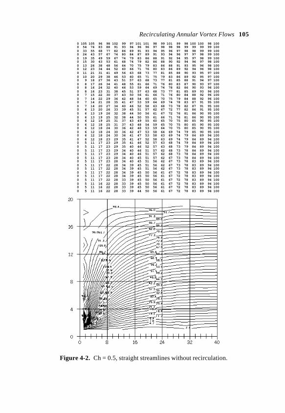
Recirculating Annular Vortex Flows 1050 105 105 96 98 102 99 97 101 101 98 99 101 99 98 100 100 98 1000 54 74 83 88 91 93 94 96 96 97 98 98 98 99 99 99 99 1000 33 55 68 77 82 86 89 91 93 94 95 96 97 98 98 99 99 1000 24 43 57 67 74 80 84 87 89 91 93 94 96 97 97 98 99 1000 19 35 49 59 67 74 79 83 86 88 91 92 94 95 97 98 99 1000 15 30 43 53 61 68 74 79 82 86 88 90 92 94 96 97 98 1000 13 26 38 48 56 64 70 75 79 83 86 88 91 93 95 96 98 1000 12 23 34 44 52 60 66 71 76 80 83 86 89 92 94 96 98 1000 11 21 31 41 49 56 63 68 73 77 81 85 88 90 93 95 97 1000 10 20 29 38 46 53 60 65 71 75 79 83 86 89 92 95 97 1000 9 18 27 36 43 51 57 63 68 73 77 81 85 88 91 94 97 1000 8 17 26 34 41 48 55 61 66 71 76 80 83 87 90 93 97 1000 8 16 24 32 40 46 53 59 64 69 74 78 82 86 90 93 96 1000 8 16 23 31 38 45 51 57 63 68 73 77 81 85 89 93 96 1000 7 15 22 30 37 43 50 56 61 66 71 76 80 84 88 92 96 1000 7 14 22 29 36 42 48 54 60 65 70 75 79 84 88 92 96 1000 7 14 21 28 35 41 47 53 59 64 69 74 78 83 87 91 95 1000 7 14 20 27 34 40 46 52 58 63 68 73 78 82 87 91 95 1000 6 13 20 26 33 39 45 51 57 62 67 72 77 82 86 91 95 1000 6 13 19 26 32 38 44 50 56 61 67 72 76 81 86 90 95 1000 6 13 19 25 32 38 44 50 55 61 66 71 76 81 86 90 95 1000 6 12 19 25 31 37 43 49 55 60 65 70 75 80 85 90 95 1000 6 12 18 25 31 37 43 48 54 59 65 70 75 80 85 90 95 1000 6 12 18 24 30 36 42 48 53 59 64 70 75 80 85 90 95 1000 6 12 18 24 30 36 42 47 53 58 64 69 74 79 85 90 95 1000 6 12 18 24 30 36 41 47 53 58 63 69 74 79 84 89 94 1000 6 12 18 23 29 35 41 47 52 58 63 69 74 79 84 89 94 1000 5 11 17 23 29 35 41 46 52 57 63 68 74 79 84 89 94 1000 5 11 17 23 29 35 40 46 52 57 63 68 73 79 84 89 94 1000 5 11 17 23 29 34 40 46 51 57 62 68 73 78 84 89 94 1000 5 11 17 23 29 34 40 46 51 57 62 68 73 78 84 89 94 1000 5 11 17 23 28 34 40 45 51 57 62 67 73 78 84 89 94 1000 5 11 17 23 28 34 40 45 51 56 62 67 73 78 83 89 94 1000 5 11 17 22 28 34 39 45 51 56 62 67 73 78 83 89 94 1000 5 11 17 22 28 34 39 45 51 56 62 67 73 78 83 89 94 1000 5 11 17 22 28 34 39 45 50 56 61 67 72 78 83 89 94 1000 5 11 17 22 28 34 39 45 50 56 61 67 72 78 83 89 94 1000 5 11 17 22 28 33 39 45 50 56 61 67 72 78 83 89 94 1000 5 11 16 22 28 33 39 45 50 56 61 67 72 78 83 89 94 1000 5 11 16 22 28 33 39 45 50 56 61 67 72 78 83 89 94 1000 5 11 16 22 28 33 39 44 50 56 61 67 72 78 83 89 94 100
Figure 4-2. Ch = 0.5, straight streamlines without recirculation.
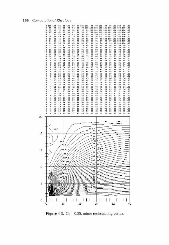
106 Computational Rheology0 105 105 96 98 102 99 97 101 101 98 99 101 99 98 100 100 98 1000 55 76 85 90 94 96 98 99 100 100 100 101 101 100 100 100 100 1000 35 58 72 81 87 92 95 97 99 100 101 101 101 101 101 100 100 1000 25 47 62 73 81 87 92 95 97 99 100 101 101 101 101 101 100 1000 21 39 55 66 76 83 88 92 95 98 99 100 101 101 101 101 100 1000 18 34 49 61 71 79 85 90 93 96 98 100 100 101 101 100 100 1000 16 31 45 57 67 75 82 87 91 94 97 99 100 100 100 100 100 1000 14 28 41 53 63 71 78 84 89 93 95 97 99 99 100 100 100 1000 13 26 39 50 60 68 76 82 87 91 94 96 98 99 99 100 100 1000 12 25 37 47 57 66 73 79 85 89 92 95 96 98 99 99 99 1000 12 23 35 45 55 63 71 77 82 87 90 93 95 97 98 99 99 1000 11 22 33 43 53 61 68 75 80 85 89 92 94 96 97 98 99 1000 11 21 32 42 51 59 66 73 78 83 87 90 93 95 96 98 99 1000 10 21 31 40 49 57 64 71 77 82 86 89 92 94 96 97 98 1000 10 20 30 39 47 55 63 69 75 80 84 88 91 93 95 97 98 1000 9 19 29 38 46 54 61 68 73 78 83 86 90 92 94 96 98 1000 9 19 28 36 45 53 60 66 72 77 81 85 89 91 94 96 98 1000 9 18 27 35 44 51 58 65 70 76 80 84 88 90 93 95 97 1000 9 17 26 35 43 50 57 63 69 74 79 83 87 90 92 95 97 1000 8 17 26 34 42 49 56 62 68 73 78 82 86 89 92 95 97 1000 8 17 25 33 41 48 55 61 67 72 77 81 85 88 91 94 97 1000 8 16 24 32 40 47 54 60 66 71 76 80 84 88 91 94 97 1000 8 16 24 32 39 46 53 59 65 70 75 79 83 87 90 94 97 1000 8 15 23 31 38 45 52 58 64 69 74 78 83 86 90 93 96 1000 7 15 23 30 37 44 51 57 63 68 73 78 82 86 89 93 96 1000 7 15 22 30 37 44 50 56 62 67 72 77 81 85 89 93 96 1000 7 15 22 29 36 43 49 55 61 67 72 76 81 85 89 92 96 1000 7 14 22 29 36 42 49 55 60 66 71 76 80 84 88 92 96 1000 7 14 21 28 35 42 48 54 60 65 70 75 80 84 88 92 96 1000 7 14 21 28 35 41 47 53 59 64 70 74 79 83 88 92 96 1000 7 14 21 27 34 41 47 53 58 64 69 74 79 83 87 91 96 1000 7 13 20 27 34 40 46 52 58 63 69 73 78 83 87 91 95 1000 6 13 20 27 33 40 46 52 57 63 68 73 78 82 87 91 95 1000 6 13 20 26 33 39 45 51 57 62 68 73 77 82 87 91 95 1000 6 13 20 26 33 39 45 51 56 62 67 72 77 82 86 91 95 1000 6 13 19 26 32 38 44 50 56 61 67 72 77 81 86 91 95 1000 6 13 19 26 32 38 44 50 56 61 66 71 76 81 86 90 95 1000 6 13 19 25 32 38 44 50 55 61 66 71 76 81 86 90 95 1000 6 12 19 25 31 37 43 49 55 60 66 71 76 81 85 90 95 1000 6 12 19 25 31 37 43 49 54 60 65 70 76 80 85 90 95 1000 6 12 19 25 31 37 43 49 54 60 65 70 75 80 85 90 95 100
Figure 4-3. Ch = 0.35, minor recirculating vortex.

Recirculating Annular Vortex Flows 1070 105 105 96 98 102 99 97 101 101 98 99 101 99 98 100 100 98 1000 55 77 87 93 96 99 100 102 102 103 103 103 103 102 102 101 100 1000 36 60 75 85 92 97 100 103 104 105 106 106 105 104 103 102 101 1000 27 50 67 79 88 95 100 103 106 107 108 108 107 106 105 103 101 1000 23 43 60 74 84 92 98 103 106 108 109 109 109 108 106 104 102 1000 20 39 56 70 81 90 97 102 106 109 110 110 110 109 107 105 102 1000 18 36 52 66 78 88 96 102 106 109 111 111 111 109 108 105 102 1000 17 34 50 64 76 86 94 101 105 109 111 111 111 110 108 105 103 1000 16 33 48 62 74 84 93 100 105 108 111 112 111 110 108 106 103 1000 16 32 47 60 72 83 92 99 104 108 110 112 111 110 108 106 103 1000 15 31 45 59 71 82 90 98 103 108 110 111 111 110 108 106 103 1000 15 30 44 58 70 80 89 97 103 107 110 111 111 110 108 106 103 1000 15 29 44 57 69 79 88 96 102 106 109 111 111 110 108 106 103 1000 14 29 43 56 68 78 87 95 101 106 109 110 110 110 108 106 103 1000 14 28 42 55 67 77 87 94 100 105 108 110 110 109 108 105 103 1000 14 28 42 54 66 77 86 93 99 104 107 109 110 109 107 105 102 1000 14 28 41 54 65 76 85 93 99 103 107 108 109 109 107 105 102 1000 14 27 41 53 65 75 84 92 98 103 106 108 109 108 107 105 102 1000 13 27 40 53 64 74 83 91 97 102 105 107 108 108 106 105 102 1000 13 27 40 52 63 74 83 90 96 101 105 107 107 107 106 104 102 1000 13 26 39 52 63 73 82 89 96 100 104 106 107 107 106 104 102 1000 13 26 39 51 62 72 81 89 95 100 103 105 106 106 105 104 102 1000 13 26 39 51 62 72 80 88 94 99 103 105 106 106 105 104 102 1000 13 26 38 50 61 71 80 87 93 98 102 104 105 105 105 103 102 1000 13 25 38 50 60 70 79 87 93 98 101 104 105 105 104 103 101 1000 12 25 37 49 60 70 78 86 92 97 101 103 104 105 104 103 101 1000 12 25 37 49 59 69 78 85 91 96 100 102 104 104 104 103 101 1000 12 25 37 48 59 69 77 85 91 96 99 102 103 104 103 102 101 1000 12 24 36 48 58 68 76 84 90 95 99 101 103 103 103 102 101 1000 12 24 36 47 58 67 76 83 89 94 98 101 102 103 103 102 101 1000 12 24 36 47 57 67 75 83 89 94 97 100 102 102 102 102 101 1000 12 24 35 47 57 66 75 82 88 93 97 100 101 102 102 102 101 1000 12 24 35 46 56 66 74 81 88 92 96 99 101 102 102 101 101 1000 12 23 35 46 56 65 74 81 87 92 96 99 100 101 102 101 100 1000 11 23 35 45 55 65 73 80 86 91 95 98 100 101 101 101 100 1000 11 23 34 45 55 64 72 80 86 91 95 98 99 101 101 101 100 1000 11 23 34 45 55 64 72 79 85 90 94 97 99 100 101 101 100 1000 11 23 34 44 54 63 71 78 85 90 94 97 99 100 100 100 100 1000 11 22 33 44 54 63 71 78 84 89 93 96 98 99 100 100 100 1000 11 22 33 44 53 62 70 77 83 88 93 96 98 99 100 100 100 1000 11 22 33 43 53 62 70 77 83 88 92 95 97 99 100 100 100 100
Figure 4-4. Ch = 0.320, large scale recirculation.

108 Computational Rheology0 105 105 96 98 102 99 97 101 101 98 99 101 99 98 100 100 98 1000 55 77 87 93 97 99 101 102 103 103 103 103 103 102 102 101 100 1000 36 61 76 86 93 98 101 104 105 106 106 106 106 105 104 102 101 1000 27 50 67 80 89 96 101 104 107 108 109 109 108 107 105 104 102 1000 23 44 61 75 85 93 100 104 107 109 110 111 110 109 107 105 102 1000 20 40 57 71 82 91 99 104 108 110 112 112 111 110 108 105 102 1000 19 37 53 68 80 90 97 104 108 111 112 113 112 111 109 106 103 1000 18 35 51 65 78 88 96 103 108 111 113 114 113 111 109 106 103 1000 17 34 49 63 76 87 95 102 108 111 113 114 113 112 110 107 103 1000 16 33 48 62 75 85 94 102 107 111 113 114 114 112 110 107 103 1000 16 32 47 61 73 84 94 101 107 111 113 114 114 112 110 107 103 1000 16 31 46 60 72 83 93 100 106 110 113 114 114 112 110 107 103 1000 15 31 45 59 72 83 92 100 106 110 113 114 114 112 110 107 103 1000 15 30 45 58 71 82 91 99 105 110 112 114 113 112 110 107 103 1000 15 30 44 58 70 81 91 98 105 109 112 113 113 112 110 107 103 1000 15 30 44 57 70 81 90 98 104 109 111 113 113 112 110 107 103 1000 15 29 44 57 69 80 89 97 103 108 111 113 113 112 109 107 103 1000 14 29 43 56 69 79 89 97 103 108 111 112 112 111 109 106 103 1000 14 29 43 56 68 79 88 96 102 107 110 112 112 111 109 106 103 1000 14 29 42 56 68 78 88 96 102 107 110 111 112 111 109 106 103 1000 14 28 42 55 67 78 87 95 101 106 109 111 111 110 109 106 103 1000 14 28 42 55 67 77 87 94 101 105 109 110 111 110 108 106 103 1000 14 28 42 54 66 77 86 94 100 105 108 110 111 110 108 106 103 1000 14 28 41 54 66 76 86 93 100 104 108 110 110 109 108 106 103 1000 14 28 41 54 65 76 85 93 99 104 107 109 110 109 108 105 103 1000 14 27 41 53 65 75 85 92 99 103 107 109 109 109 107 105 102 1000 14 27 41 53 65 75 84 92 98 103 106 108 109 109 107 105 102 1000 13 27 40 53 64 75 84 91 98 102 106 108 109 108 107 105 102 1000 13 27 40 52 64 74 83 91 97 102 105 107 108 108 107 105 102 1000 13 27 40 52 63 74 83 90 97 102 105 107 108 108 106 105 102 1000 13 27 40 52 63 73 82 90 96 101 104 107 107 107 106 104 102 1000 13 26 39 51 63 73 82 89 96 101 104 106 107 107 106 104 102 1000 13 26 39 51 62 72 81 89 95 100 104 106 107 107 106 104 102 1000 13 26 39 51 62 72 81 89 95 100 103 105 106 106 105 104 102 1000 13 26 39 51 62 72 81 88 94 99 103 105 106 106 105 104 102 1000 13 26 38 50 61 71 80 88 94 99 102 105 106 106 105 104 102 1000 13 26 38 50 61 71 80 87 93 98 102 104 105 105 105 103 102 1000 13 25 38 50 61 70 79 87 93 98 101 104 105 105 105 103 101 1000 13 25 38 49 60 70 79 86 93 97 101 103 105 105 104 103 101 1000 12 25 37 49 60 70 78 86 92 97 101 103 104 105 104 103 101 1000 12 25 37 49 60 69 78 85 92 97 100 103 104 104 104 103 101 100
Figure 4-5. Ch = 0.319, major flow blockage.
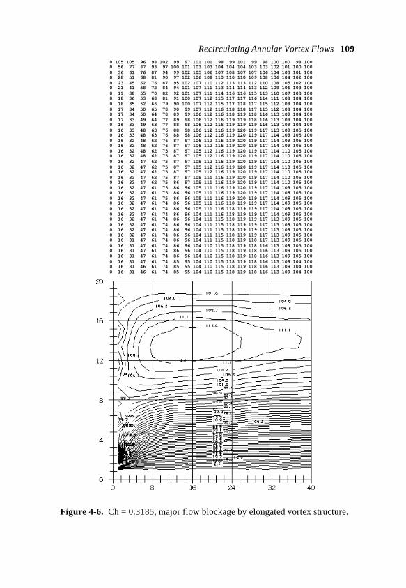
Recirculating Annular Vortex Flows 1090 105 105 96 98 102 99 97 101 101 98 99 101 99 98 100 100 98 1000 56 77 87 93 97 100 101 103 103 104 104 104 103 103 102 101 100 1000 36 61 76 87 94 99 102 105 106 107 108 107 107 106 104 103 101 1000 28 51 68 81 90 97 102 106 108 110 110 110 109 108 106 104 102 1000 23 45 62 76 87 95 102 107 110 112 113 113 112 110 108 105 102 1000 21 41 58 72 84 94 101 107 111 113 114 114 113 112 109 106 103 1000 19 38 55 70 82 92 101 107 111 114 116 116 115 113 110 107 103 1000 18 36 53 68 81 91 100 107 112 115 117 117 116 114 111 108 104 1000 18 35 52 66 79 90 100 107 112 115 117 118 117 115 112 108 104 1000 17 34 50 65 78 90 99 107 112 116 118 118 117 115 112 108 104 1000 17 34 50 64 78 89 99 106 112 116 118 119 118 116 113 109 104 1000 17 33 49 64 77 89 98 106 112 116 119 119 118 116 113 109 104 1000 16 33 49 63 77 88 98 106 112 116 119 119 119 116 113 109 104 1000 16 33 48 63 76 88 98 106 112 116 119 120 119 117 113 109 105 1000 16 33 48 63 76 88 98 106 112 116 119 120 119 117 114 109 105 1000 16 32 48 62 76 87 97 106 112 116 119 120 119 117 114 109 105 1000 16 32 48 62 76 87 97 106 112 116 119 120 119 117 114 109 105 1000 16 32 48 62 75 87 97 105 112 116 119 120 119 117 114 110 105 1000 16 32 48 62 75 87 97 105 112 116 119 120 119 117 114 110 105 1000 16 32 47 62 75 87 97 105 112 116 119 120 119 117 114 110 105 1000 16 32 47 62 75 87 97 105 112 116 119 120 119 117 114 110 105 1000 16 32 47 62 75 87 97 105 112 116 119 120 119 117 114 110 105 1000 16 32 47 62 75 87 97 105 111 116 119 120 119 117 114 110 105 1000 16 32 47 62 75 86 97 105 111 116 119 120 119 117 114 110 105 1000 16 32 47 61 75 86 96 105 111 116 119 120 119 117 114 109 105 1000 16 32 47 61 75 86 96 105 111 116 119 120 119 117 114 109 105 1000 16 32 47 61 75 86 96 105 111 116 119 120 119 117 114 109 105 1000 16 32 47 61 74 86 96 105 111 116 118 119 119 117 114 109 105 1000 16 32 47 61 74 86 96 105 111 116 118 119 119 117 114 109 105 1000 16 32 47 61 74 86 96 104 111 116 118 119 119 117 114 109 105 1000 16 32 47 61 74 86 96 104 111 115 118 119 119 117 113 109 105 1000 16 32 47 61 74 86 96 104 111 115 118 119 119 117 113 109 105 1000 16 32 47 61 74 86 96 104 111 115 118 119 119 117 113 109 105 1000 16 32 47 61 74 86 96 104 111 115 118 119 119 117 113 109 105 1000 16 31 47 61 74 86 96 104 111 115 118 119 118 117 113 109 105 1000 16 31 47 61 74 86 96 104 110 115 118 119 118 116 113 109 105 1000 16 31 47 61 74 86 96 104 110 115 118 119 118 116 113 109 105 1000 16 31 47 61 74 86 96 104 110 115 118 119 118 116 113 109 105 1000 16 31 47 61 74 85 95 104 110 115 118 119 118 116 113 109 104 1000 16 31 46 61 74 85 95 104 110 115 118 119 118 116 113 109 104 1000 16 31 46 61 74 85 95 104 110 115 118 119 118 116 113 109 104 100
Figure 4-6. Ch = 0.3185, major flow blockage by elongated vortex structure.
110 Computational Rheology
HOW TO AVOID STAGNANT BUBBLES
We have shown that recirculating zones can develop from interactionsbetween inertia and gravity forces. These bubbles form when densitystratification, hole deviation and pump rate fulfill certain special conditions.These are elegantly captured in a single channel variable, the nondimensional
parameter Ch = U2ρref /gLdρ cos α. Moreover, the resulting flowfields can be
efficiently computed and displayed, thus allowing us to understand better theirdynamical consequences.
Suppressing recirculating flows is simply accomplished: avoid smallvalues of the nondimensional Ch parameter. Small values, as is evident fromEquation 4-4, can result from different isolated effects. For example, itdecreases as the hole becomes more horizontal, as density differences becomemore pronounced, or as pumping rates decrease. But none of these factors alonecontrol the physics; it is the combination taken together that controls bubbleformation and perhaps the fate of a drilling program.
We have modeled the problem as the single phase flow of a stratified fluid,rather than as the combined motion of dual-phase fluid and solid continuum.This simplifies the mathematical issues without sacrificing the essential physicaldetails. For practical purposes, the parameter Ch can be viewed as a “dangerindicator” signaling impending cuttings transport or stuck pipe problems. It isthe single most important parameter whenever interrupted circulation or poorsuspension properties lead to gravity segregation and settling of weightingmaterials in drilling mud.
These considerations also apply to cementing, where density segregationdue to gravity and slow velocities are both likely. When recirculation zonesform in either the mud or the cement above or beneath the casing, thedisplacement effectiveness of the cement is severely impeded. The result is mudleft in place, an undesirable one necessitating squeeze jobs. Similar remarksapply to pipeline applications. Recirculation zones are likely to be encounteredat low flow rates that promote density stratification, and immediately prior toflow start-up, when slurry particles have been allowed to settle out.
We emphasize that the vortical bubbles considered here are not the “Taylorvortices” studied in the classical fluid mechanics of homogeneous flows. Taylorvortices are “doughnuts” that would normally “wrap around,” in our case, thedrillpipe; to the author’s knowledge, these have not been observed in drillingapplications. They can be created in the absence of density stratification, that is,they can be found in purely homogeneous fluids. Importantly, Taylor vorticeswould owe their existence to finite drillstring length effects, and would representcompletely different physical mechanisms.

Applications to Drilling and Production 111
A PRACTICAL EXAMPLE
We have discussed the dynamical significance of the nondimensionalparameter Ch that appears in the normalized equations of motion. For use inpractical estimates, the channel variable may be written more clearly as amultiplicative sequence of dimensionless entities,
Ch = U2ρref /gLdρ cos α (4-5)
= (U2/gL) × (ρref / dρ) × (1/cos α)
Let us consider an annular flow studied in the cuttings transport examplesof Chapter 5. For the 2-inch and 5-inch pipe and borehole radii, the cross-
sectional area is π (52 -22) or 66 in2.The experimental data used in Discussions 1 and 2 of Chapter 5 assume
oncoming linear velocities of 1.91, 2.86 and 3.82 ft/sec. Since 1 ft/sec
corresponds to a volume flow rate of 1 ft/sec × 66 in2 or 205.7 gpm, the flowrates are 393, 588 and 786 gpm. So, at the lowest flow rate of 393 gpm (areasonable field number), the average linear speed over the entire annulus isapproximately 2 ft/sec. But the low-side average will be much smaller, say 0.5ft/sec. And if the pipe is displaced halfway down, the length scale L will beroughly (5-2) /2 inches or 0.13 ft.
Thus, the first factor in Equation 4-5 takes the value U2/gL = (0.5)2/(32.2× 0.13) = 0.06. If we assume a 20% density stratification, then ρref /dρ = 5.0;
the product of the two factors is 0.30. For a highly deviated well inclined 70o
from the vertical axis, α = 90o - 70o = 20o and cos 20o = 0.94. Thus, we obtainCh = 0.30/0.94 = 0.32. This value, as Figures 4-1 to 4-6 show, lies just at thethreshold of danger. Velocities lower than the assumed value are even morelikely to sustain recirculatory flows; higher ones, in contrast, are safer.
Of course, the numbers used above are only estimates; a three-dimensional,viscous solution is required to establish true length and velocity scales. Butthese approximate results show that bottomhole conditions typical of those usedin drilling and cementing are associated with low values of Ch near unity.
We emphasize that Ch is the only nondimensional parameter appearing inEquations 4-1 to 4-3. Another one describing the geometry of the annulardomain would normally appear through boundary conditions. For conveniencethough (and for the sake of argument only), we have replaced this requirementwith an idealized “sink.” In any real calculation, exact geometrical effects mustbe included to complete the formulation. Also note that our recirculating flowsget worse as the borehole becomes more horizontal; that is, Ch decreases as αbecomes smaller. This is in stark contrast to the unidirectional, homogeneous
112 Computational Rheology
flows of Chapter 5, which, as we will prove, perform worst near 45o, at leastwith respect to cuttings transport efficiency. The structure of Equation 4-4
correctly shows that in near-vertical wells with α approaching 90o, Ch tends toinfinity; thus, the effects of flow blockage due to the vortical bubbles consideredhere are relegated to highly deviated wells.
Again, flow properties such as local velocity, shear rate, and pressure canbe obtained from the computed streamfunction straightforwardly. They may beuseful correlation parameters for cuttings transport efficiency and local bedbuildup. Continuing research is underway, exploring similarities between thisproblem and the density-dependent flows studied in dynamic meteorology andoceanography. Obvious extensions of our observations for annular flow applyto the pipeline transport of wax and hydrate slurries.
REFERENCES
Schlichting, H., Boundary Layer Theory, McGraw-Hill, New York, 1968.
Turner, J.S., Buoyancy Effects in Fluids, Cambridge University Press, London,1973.
113
5
Applications to Drilling and Production
In Chapters 2, 3, and 4, we formulated and solved three distinct annularflow models and gave numerous calculated results. These models remove manyof the restrictions usually made regarding eccentricity, rotation, and flowhomogeneity. The methods also produce fast and stable solutions, with highlydetailed output processing. Unfortunately, it is not yet possible to build a singlemodel for rotating, inhomogeneous flow in eccentric domains. This chapterdeals with practical applications of these models in drilling and production.Topics discussed include cuttings transport in deviated holes, stuck pipeevaluation, cementing, and coiled tubing return flow analysis. For the casualreader, brief summaries of the three models are offered first.
Recapitulation. Let us briefly summarize the modeling capabilitiesdeveloped. The first annular flow model applies to homogeneous Newtonian,power law, Bingham plastic, and Herschel-Bulkley fluids. It assumes anonrotating drillpipe (or casing) in an inclined hole, but no restrictions areplaced on the annular geometry itself. The unidirectional analysis handleseccentric circular drillpipes and boreholes; but it also models, with no extradifficulty or computational expense, deformed borehole walls due to erosion,swelling or cuttings bed buildup, and, for example, square drill collars withstabilizers. A description of this capability was first offered in Chin (1990a).
The exact PDEs are solved on boundary conforming grid systems thatyield high resolution in tight spaces. They handle geometry exactly, so that slotflow and bipolar coordinate approximations are unnecessary. Theunconditionally stable finite difference program, requiring five seconds persimulation on Pentium machines, has been successfully executed thousands oftimes without diverging since the original publication.
114 Computational Rheology
To help understand the lengthy output, which includes annular velocity,apparent viscosity, two components of viscous stress and shear rate, Stokesproduct and dissipation function, a special character-based graphics programwas developed. This utility overlays results on the annular geometry itself, thusfacilitating physical interpretation and visual correlation of computed quantitieswith annular position. The algorithms and graphics software are written instandard Fortran; they are easily ported to most hardware platforms withminimal modification. Calculations and displays for several difficult geometriesare given in Chapter 2. With the present revision, more sophisticated colorgraphics capabilities are available, but the original text diagrams still provide the“quantitative feeling” necessary in understanding engineering problems.
The second flow model provides approximate analytical solutions forpower law fluids in concentric annular flows containing rotating drillstrings orcasings. Here, a “narrow annulus” assumption is invoked; hole inclination, as inthe first model, scales out by using a normalized pressure. Closed formsolutions are derived for axial and circumferential velocity, pressure, viscousstress, deformation rate, apparent viscosity and local heat generation. All theproperties listed are given as explicit functions of the radial coordinate “r.”Again, built-in, portable graphical utilities permit quick, convenient displays ofall relevant flow parameters. The corresponding solutions for Newtonian floware also given in closed analytical form, but no restrictions on annular geometryare required; here, the solutions satisfy the Navier-Stokes equations exactly.
The third and final model considers density heterogeneities due to “baritesag,” or, more generally, gravity stratification. This opens up the possibility ofreversed flow in the axial direction, and annular blockage of an entirely fluid-dynamical nature. This recirculating flow is to be contrasted with better knownsecondary vortex flows that occur in the cross-sectional planes of pipes. Unlikethe latter, which are controlled by viscosity, analysis shows that the existence ofbarite “trapped bubbles” depends on a single nondimensional parameter that isindependent of the stress versus strain relation.
The fluid density “ρ” does not explicitly appear in the momentumequations for the first two models, because geometrical simplifications eliminatethe convective term associated with “F = ma.” The influence of “mud weight”appears indirectly, only through its rheological effect on n, k, and yield strength.On the other hand, rheology (to be precise, the exact stress versus strain relation)does not play a fundamental role in sag-induced bubbles; flow reversals due togravity segregation are primarily inertia dominated. Of course, flows can befound that run counter to our assumptions; however, the author believes that themodels chosen for exposition correctly describe physical problems in actualdrilling and production.
Applications to Drilling and Production 115
CUTTINGS TRANSPORT IN DEVIATED WELLS
Recent industry interest in horizontal and highly deviated wells hasheightened the importance of annular flow modeling as it relates to holecleaning. Cuttings transport to the surface is generally impeded by virtue ofhole orientation; this is worsened by decreased “low-side” annular velocities dueto pipe eccentricity. In addition, the blockage created by bed buildup decreasesoverall flow rate, further reducing cleaning efficiency. In what could possiblybe a self-sustaining, destabilizing process, stuck pipe is a likely end result. Thissection discloses new cuttings transport correlations and suggests simplepredictive measures to avoid bed buildup. Good hole cleaning and bed removal,of course, are important to cementing as well.
Few useful annular flow models are available despite their practicalimportance. The nonlinear equations governing power law viscous fluids, forexample, must be solved with difficult no-slip conditions for highly eccentricgeometries. Recent slot flow models offer some improvement over parallelplate approaches. Still, because they unrealistically require slow radialvariations in the circumferential direction, large errors are possible. Even whenthey apply, these models can be cumbersome; they involve “elliptic integrals,”which are too awkward for field use. Bipolar coordinate models accuratelysimulate eccentric flows with circular pipes and boreholes; however, they cannotbe extended to real world applications containing washouts and cuttings beds.
In this section, the eccentric flow model is used to interpret field andlaboratory results. Because the model actually simulates reality, it has beenpossible to correlate problems associated with cuttings transport and stuck pipeto unique average mechanical properties of the computed flowfield. Thesecorrelations are discussed next.
Discussion 1. Water-Base Muds
Detailed computations using the eccentric model are described, assuming apower law fluid, which correspond to the comprehensive suite of cuttingstransport experiments conducted at the University of Tulsa (Becker, Azar andOkrajni, 1989). For a fixed inclination and oncoming flow rate, we importantlydemonstrate that “cuttings concentration” correlates linearly with the meanviscous shear stress averaged over the lower half of the annulus. Thus,impending cuttings problems can be eased by first determining the existingaverage stress level; and then, adjusting n, k, and gpm values to increase thatstress. Physical arguments supporting our correlations will be given. Weemphasize that the present approach is completely predictive and deterministic;
116 Computational Rheology
it does not require empirical assumptions related to the “equivalent hydraulicradius” or to questionable “pipe to annulus conversion factors.” This result wasfirst reported in Chin (1990b), and the “stress correlation” is now used in severalservice company models for cuttings transport application.
Detailed experimental results for cuttings concentration, a useful indicatorof transport efficiency and carrying capacity, were obtained at the University ofTulsa’s large scale flow loop. Fifteen bentonite-polymer, water-based muds, forthree average flow rates (1.91, 2.86 and 3.82 ft/sec), at three boreholeinclinations from vertical (30, 45 and 70 deg), were tested. Table 1 of Becker etal. (1989) summarizes all measured mud properties, along with specific powerlaw exponents n and consistency factors k. We emphasize that “water base”does not imply Newtonian flow; in fact, the reported values of n differsubstantially from unity. The annular geometry consisted of a 2-inch-radiuspipe, displaced downward by 1.5 inches in a 5-inch-radius borehole; also, thepipe rotated at 50 rpm.
With flow rate and hole inclination fixed, the authors cross-plot thenondimensional cuttings concentration C versus particular rheological propertiesfor each mud type used. These include apparent viscosity, plastic viscosity(PV), yield point (YP), YP/PV, initial and ten-minute gel strength, “effectiveviscosity,” k, and Fann dial readings at various rpms. Typically, the correlationsobtained were poor, with one exception to be discussed. That good correlationswere not possible, of course, is not surprising; the “fluid properties” in Becker etal. (1989) are rotational viscometer readings describing the test instrument only.That is, they have no real bearing to the actual annular geometry and itsdownhole flow, which from Chapter 2 we understand can be complicated.
These cross-plots and tables, numbering over 20, were nevertheless studiedin detail; using them, the entire laboratory database was reconstructed. Theconcentric, rotating flow program described in Chapter 3 was run to show thatrpm effects were likely to be insignificant. The eccentric annular model ofChapter 2 was then executed for each of the 135 experimental points; detailedresults for calculated apparent viscosity, shear rate, viscous stress and axialvelocity, all of which varied spatially, were tabulated and statistically analyzedalong with the experimental data.
Numerous cross-plots were produced, examined, and interpreted. Themost meaningful correlation parameter found was the mean viscous shear stress,obtained by averaging computed values over the bottom half of the annulus,where cuttings in directional wells are known to form beds. Figures 5-1, 5-2,and 5-3 display cuttings concentration versus our mean shear stress for differentaverage flow speeds and inclination angles ß from the vertical. Each plottedsymbol represents a distinct test mud. Calculated correlation coefficientsaveraged a high 0.91 value. Our correlations apply to laminar flow only; theflattened portions of the curves refer to turbulent conditions. Computationally,the latter are simulated with a subroutine change to include turbulence modeling.

Applications to Drilling and Production 117
Mea
n St
ress
(ps
i)
1.91
ft/s
ec
2.86
ft/s
ec
3.82
ft/s
ec
0
1
2
3
4 x
10
- 4
023410111213
341415163031
8913142122C
%
β =
30
oβ
= 4
5 o
β =
70
o
Fig
ures
5-1
, 2, 3
. C
uttin
gs tr
ansp
ort c
orre
latio
n.
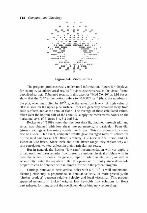
118 Computational Rheology55 57 55
49 45 47 45 49
39 39 28 29 28 39 39 30 24 13 24 30 27 12 12 27 17 9 4 4 4 9 17 19 4 6 18 18 18 6 4 19 12 8 9 19 31 31 31 19 9 8 12 1 19 30 44 5844 30 19 1 6 12 28 5169 7269 513628 12 6 0 8 1924 436280 8380706243 2419 8 0 1 1519 293250 555029 1915 1 5 9 20 35 37352020 9 5 1315 2018 1920 1513 14 1514 8 4111415 14 151517 1 1 15171515 13 8 212 7 313 23222018 9 210 21 3 21418202223 21 2621 1511 21518 2918 9 415 2725 0 15 1815 6 0 212527 2419 5 8 5 141924 28 15 13 15 28 2622 20 26 24
Figure 5-4. Viscous stress.
The program produces easily understood information. Figure 5-4 displays,for example, calculated areal results for viscous shear stress in the visual formatdescribed earlier. Tabulated results, in this case for “Mud No. 10” at 1.91 ft/sec,show that the “24” at the bottom refers to “0.00024 psi” (thus, the numbers in
the plot, when multiplied by 10-5, give the actual psi level). A high value of“83” is seen on the upper pipe surface; lows are generally obtained away fromsolid surfaces and at the annular floor. The average of these calculated values,taken over the bottom half of the annulus, supply the mean stress points on thehorizontal axes of Figures 5-1, 5-2 and 5-3.
Becker et al (1989) noted that the best data fit, obtained through trial anderror, was obtained with low shear rate parameters, in particular, Fann dial(stress) readings at low rotary speeds like 6 rpm. This corresponds to a shearrate of 10/sec. Our exact, computed results gave averaged rates of 7-9/sec forall the mud samples at 1.91 ft/sec; similarly, 11-14/sec at 2.86 ft/sec, and 14-19/sec at 3.82 ft/sec. Since these are in the 10/sec range, they explain why a 6rpm correlation worked, at least in their particular test setup.
But in general, the Becker “low rpm” recommendation will not apply apriori; each nonlinear annular flow presents a unique physical problem with itsown characteristic shears. In general, pipe to hole diameter ratio, as well aseccentricity, enter the equation. But this poses no difficulty since downholeproperties can be obtained with minimal effort with the present program.
Cuttings removal in near-vertical holes with ß < 10o is well understood;cleaning efficiency is proportional to annular velocity, or more precisely, the“Stokes product” between relative velocity and local viscosity. This productappeared naturally in Stokes’ original low Reynolds flow solutions for flowspast spheres, forming part of the coefficient describing net viscous drag.

Applications to Drilling and Production 119
For inclined wells, the usual notions regarding unimpeded settlingvelocities do not apply because different physical processes are at work.Cuttings travel almost immediately to the low side of the annulus, aconsequence of gravity segregation; they remain there and form beds that mayor may not slide downward. These truss or lattice-like structures have welldefined mechanical yield stresses; the right amount of viscous friction will erodethe cuttings bed, the same way mud circulation limits dynamic filter cakegrowth. This explains our success in using bottom-averaged viscous stress asthe correlation parameter. The straight line fit also indicates that bed propertiesare linear in an elastic sense.
These ideas, of course, are not entirely new. Slurry pipeline designers, forexample, routinely consider “boundary shear” and “critical tractive force.” Theyhave successfully modeled sediment beds as “series of superposed layers” withdistinct yield strengths (Streeter, 1961). However, these studies are usuallyrestricted to Newtonian carrier fluids in circular conduits.
While viscous shear emerges as the dominant transport parameter, its rolewas by no mean obvious at the outset. Other correlation quantities testedinclude vertical and lateral components of shear rates and stresses, axialvelocity, apparent viscosity, and the Stokes product. These correlated somewhatwell, particularly at low inclinations, but shear stress almost always worked.Take apparent viscosity, for example. Whereas Figure 6 of Becker et al (1989)shows significant wide-band scatter, listing rotational viscometer values rangingfrom 1 to 50 cp, our exact computations gave good correlations with actualapparent viscosities ranging up to 300 cp. Computed viscosities expectedlyshowed no meaningful connection to the apparent viscosities given by theUniversity of Tulsa investigators, because the latter were inferred fromunrealistic Fann dial readings. This point is illustrated quantitatively later.
We emphasize that Figures 5-1, 5-2, and 5-3 are based on unweightedmuds. On a separate note, the effect of “pure changes in fluid density” shouldnot alter computed shear stresses, at least theoretically, since the convectiveterms in the governing equations vanish for straight holes. In practice, however,oilfield weighting materials are likely to alter n and k; thus, some change instress level might be anticipated. The effects of buoyancy, not treated here, willof course help without regard to changes in shear.
We have shown how cuttings concentration correlates in a satisfactorymanner with the mean viscous shear stress averaged over the lower half of theannulus. Thus, impending hole-cleaning problems can be alleviated by firstdetermining the existing average stress level, and then, adjusting n, k, and gpmvalues in the actual drilling fluid to increase that stress. Once this danger zone ispast, additives can be used to reduce shear stress and hence mud pump pressurerequirements. Simply increasing gpm may also help, although the effect ofrheology on stress is probably more significant.
120 Computational Rheology
Interestingly, Seeberger et al (1989) described an important field studywhere extremely high velocities together with very high yield points did notalleviate hole cleaning problems. They suggested that extrapolated YP valuesmay not be useful indicators of transport efficiency. Also, the authors pointed tothe importance of elevated stress levels at low shear rates in cleaning largediameter holes at high angles. They experimentally showed how oil and waterbase muds having like rheograms, despite their obvious textural or “look andfeel” differences, will clean with like efficiencies. This implies that aknowledge of n and k alone suffices in characterizing real muds.
The procedure suggested above requires minimal change to fieldoperations. Standard viscometer readings, plotted on “log-log” paper or used inhandbook formulas, still represent required information; but they should be usedto determine actual downhole properties through computer analysis. Yield pointand plastic viscosity, arising from older Bingham models, play no direct role inthe present methodology although these parameters sometimes offer usefulcorrelations. Also, results obtained from the eccentric model should beavailable in tabular form, and be accessible as software at the drilling site.
Discussion 2. Cuttings Transport Database
The viscometer properties and cuttings concentrations data for the 15 muds(at all angles and flow rates), together with exact computed results for shear rate,stress, apparent viscosity, annular speed, and Stokes product have beenassembled into a comparative database for continuing study. These detailedresults are available from the author upon request.
Tables 5-1, 5-2, and 5-3 summarize bottom-averaged results for theeccentric hole used in the Tulsa experiments. Computations show that thebottom of the hole supports a low shear rate flow, ranging from 10 to 20reciprocal seconds. These values are consistent with the authors’ low shear rateconclusions, established by trial and error from the experimental data. However,their rule of thumb is not universally correct; for example, the same muds andflow rates gave high shear rate results for several different downhole geometries.
Shear rates can vary substantially depending on eccentricity and diameterratio. Direct computational analysis is the only legitimate and final arbiter.These tables also give calculated apparent viscosities along with valuesextrapolated from rotating viscometer data (shown in parentheses). Comparisonshows that no correlation between the two exists, a result not unexpected, sincethe measurements bear little relation to the downhole flow. On the other hand,calculated apparent viscosities correlated well with cuttings concentration,although not as well as did viscous stress. This correlation was possible becausebottom-averaged shear rates did not vary appreciably from mud to mud at anygiven flow speed. This effect may be fortuitous.
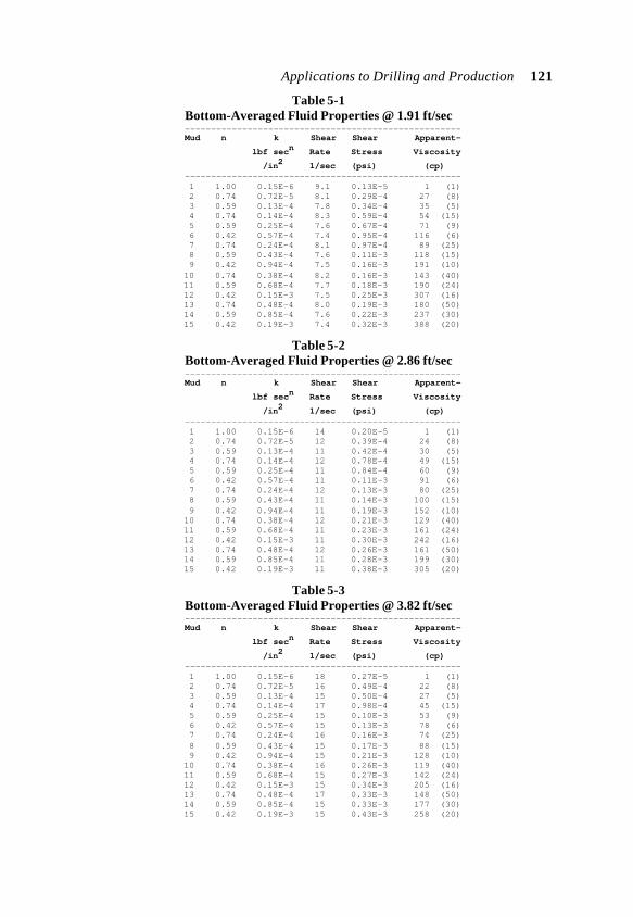
Applications to Drilling and Production 121
Table 5-1Bottom-Averaged Fluid Properties @ 1.91 ft/sec
----------------------------------------------------- Mud n k Shear Shear Apparent-
lbf secn Rate Stress Viscosity
/in2 1/sec (psi) (cp) ----------------------------------------------------- 1 1.00 0.15E-6 9.1 0.13E-5 1 (1) 2 0.74 0.72E-5 8.1 0.29E-4 27 (8) 3 0.59 0.13E-4 7.8 0.34E-4 35 (5) 4 0.74 0.14E-4 8.3 0.59E-4 54 (15) 5 0.59 0.25E-4 7.6 0.67E-4 71 (9) 6 0.42 0.57E-4 7.4 0.95E-4 116 (6) 7 0.74 0.24E-4 8.1 0.97E-4 89 (25) 8 0.59 0.43E-4 7.6 0.11E-3 118 (15) 9 0.42 0.94E-4 7.5 0.16E-3 191 (10) 10 0.74 0.38E-4 8.2 0.16E-3 143 (40) 11 0.59 0.68E-4 7.7 0.18E-3 190 (24) 12 0.42 0.15E-3 7.5 0.25E-3 307 (16) 13 0.74 0.48E-4 8.0 0.19E-3 180 (50) 14 0.59 0.85E-4 7.6 0.22E-3 237 (30) 15 0.42 0.19E-3 7.4 0.32E-3 388 (20)
Table 5-2Bottom-Averaged Fluid Properties @ 2.86 ft/sec
----------------------------------------------------- Mud n k Shear Shear Apparent-
lbf secn Rate Stress Viscosity
/in2 1/sec (psi) (cp) ----------------------------------------------------- 1 1.00 0.15E-6 14 0.20E-5 1 (1) 2 0.74 0.72E-5 12 0.39E-4 24 (8) 3 0.59 0.13E-4 11 0.42E-4 30 (5) 4 0.74 0.14E-4 12 0.78E-4 49 (15) 5 0.59 0.25E-4 11 0.84E-4 60 (9) 6 0.42 0.57E-4 11 0.11E-3 91 (6) 7 0.74 0.24E-4 12 0.13E-3 80 (25) 8 0.59 0.43E-4 11 0.14E-3 100 (15) 9 0.42 0.94E-4 11 0.19E-3 152 (10) 10 0.74 0.38E-4 12 0.21E-3 129 (40) 11 0.59 0.68E-4 11 0.23E-3 161 (24) 12 0.42 0.15E-3 11 0.30E-3 242 (16) 13 0.74 0.48E-4 12 0.26E-3 161 (50) 14 0.59 0.85E-4 11 0.28E-3 199 (30) 15 0.42 0.19E-3 11 0.38E-3 305 (20)
Table 5-3Bottom-Averaged Fluid Properties @ 3.82 ft/sec
----------------------------------------------------- Mud n k Shear Shear Apparent-
lbf secn Rate Stress Viscosity
/in2 1/sec (psi) (cp) ----------------------------------------------------- 1 1.00 0.15E-6 18 0.27E-5 1 (1) 2 0.74 0.72E-5 16 0.49E-4 22 (8) 3 0.59 0.13E-4 15 0.50E-4 27 (5) 4 0.74 0.14E-4 17 0.98E-4 45 (15) 5 0.59 0.25E-4 15 0.10E-3 53 (9) 6 0.42 0.57E-4 15 0.13E-3 78 (6) 7 0.74 0.24E-4 16 0.16E-3 74 (25) 8 0.59 0.43E-4 15 0.17E-3 88 (15) 9 0.42 0.94E-4 15 0.21E-3 128 (10) 10 0.74 0.38E-4 16 0.26E-3 119 (40) 11 0.59 0.68E-4 15 0.27E-3 142 (24) 12 0.42 0.15E-3 15 0.34E-3 205 (16) 13 0.74 0.48E-4 17 0.33E-3 148 (50) 14 0.59 0.85E-4 15 0.33E-3 177 (30) 15 0.42 0.19E-3 15 0.43E-3 258 (20)

122 Computational Rheology
Discussion 3. Invert Emulsions Versus “All Oil” Muds
Recently, Conoco’s Jolliet project successfully drilled a number of
deviated wells, ranging 30o to 60o from vertical, in the deepwater GreenCanyon Block 184 using a new “all oil” mud. Compared with wells previouslydrilled in the area with conventional invert emulsion fluids, the oil mud provedvastly superior with respect to cuttings transport and overall hole cleaning(Fraser, 1990a,b,c).
High levels of cleaning efficiency were maintained consistently throughoutthe drilling program. In this section we explain, using the fully predictive,eccentric annular flow model of Chapter 2, why the particular oil mud employedby Conoco performed well in comparison with the invert emulsion. Thefollowing discussion was first reported in Chin (1990c).
Given the success of the correlations developed in Discussion 2, it isnatural to test our “stress hypothesis” under more realistic and difficult fieldconditions. Conoco’s Green Canyon experience is ideal in this respect. Unlikethe unweighted, bentonite-polymer, water-base muds used in the University ofTulsa experiments, the drilling fluids employed by Conoco were “invertemulsion” and “all oil” muds.
Again, Seeberger et al. (1989) have demonstrated how oil-base and water-base muds having like rheograms, despite obvious textural differences, willclean holes with like efficiencies. This experimental observation implies that aknowledge of n and k alone suffices in characterizing the carrying capacity ofwater, oil-base or emulsion-base drilling fluids. Thus, the use of a power lawannular flow model as the basis for comparison for the two Conoco muds iscompletely warranted.
We assumed for simplicity a 2-inch radius drill pipe centered halfway
down a 5-inch-radius borehole. This eccentricity is consistent with the 30o to
60o inclinations reported by Conoco. The n and k values we required werecalculated from Figure 2 of Fraser (1990b), using Fann dial readings at 13 and50 rpm. For the invert emulsion, we obtained n = 0.55 and k = 0.0001 lbf
secn/sq in; the values n = 0.21 and k = 0.00055 lbf secn/sq in were found for the“all oil” mud.
Our annular geometry is identical to that used in Discussion 1 and inBecker et al. (1989). It was chosen so that the shear stress results obtained forthe Tulsa water-base muds (shown in Figures 5-1 to 5-3) can be directlycompared with those found for the weighted invert emulsion and oil fluidsconsidered here.
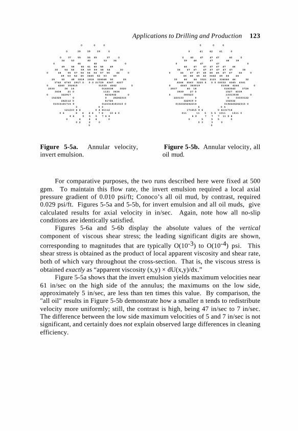
Applications to Drilling and Production 123 0 0 0
0 39 39 39 0
0 37 55 55 55 37 0 34 53 60 53 34 0 60 60 0 49 58 60 61 60 58 49 30 54 58 59 59 59 58 54 30 0 44 55 57 54 54 54 57 55 44 0 49 53 52 45 3445 52 53 49
25 50 48 3218 1818 324048 50 25 3742 4743 2917 0 0 0 01729 4347 4237 0 4240 352615 01535 4042 0 2030 36 14 0143036 3020 3434 21 0 1121 3434 0 322917 9232932 0 152326 0 0 26262315 242112 0 61724 01015181715 9 0121518181510 0 3 0 3 121210 6 4 0 4 81112 0 6 8 4 4 4 7 8 10 6 0 4 6 5 5 5 7 6 4 0 4 4 4 0 0 2 2 0 0
Figure 5-5a. Annular velocity,invert emulsion.
0 0 0
0 41 42 41 0
0 40 47 47 47 40 0 39 46 47 46 39 0 47 47 0 46 47 47 47 47 47 46 36 47 47 47 47 47 47 47 36 0 44 47 47 45 46 45 47 47 44 0 46 46 45 42 3442 45 46 46
33 46 44 3321 2121 334044 46 32 4244 4543 3220 0 0 0 02032 4345 4341 0 4443 383019 01938 4244 0 2837 40 18 0183540 3728 3939 27 0 1527 4039 0 383523 13313538 0 223133 0 0 33333122 322919 0 102532 0152325242214 0192226262315 0 5 0 5 171815 9 6 0 6131718 011 11 5 5 5 1011 1511 0 6 9 7 7 7 11 9 6 0 5 5 5 0 0 3 3 0 0
Figure 5-5b. Annular velocity, alloil mud.
For comparative purposes, the two runs described here were fixed at 500gpm. To maintain this flow rate, the invert emulsion required a local axialpressure gradient of 0.010 psi/ft; Conoco’s all oil mud, by contrast, required0.029 psi/ft. Figures 5-5a and 5-5b, for invert emulsion and all oil muds, givecalculated results for axial velocity in in/sec. Again, note how all no-slipconditions are identically satisfied.
Figures 5-6a and 5-6b display the absolute values of the verticalcomponent of viscous shear stress; the leading significant digits are shown,
corresponding to magnitudes that are typically O(10-3) to O(10-4) psi. Thisshear stress is obtained as the product of local apparent viscosity and shear rate,both of which vary throughout the cross-section. That is, the viscous stress isobtained exactly as “apparent viscosity (x,y) × dU(x,y)/dx.”
Figure 5-5a shows that the invert emulsion yields maximum velocities near61 in/sec on the high side of the annulus; the maximums on the low side,approximately 5 in/sec, are less than ten times this value. By comparison, the"all oil" results in Figure 5-5b demonstrate how a smaller n tends to redistributevelocity more uniformly; still, the contrast is high, being 47 in/sec to 7 in/sec.The difference between the low side maximum velocities of 5 and 7 in/sec is notsignificant, and certainly does not explain observed large differences in cleaningefficiency.
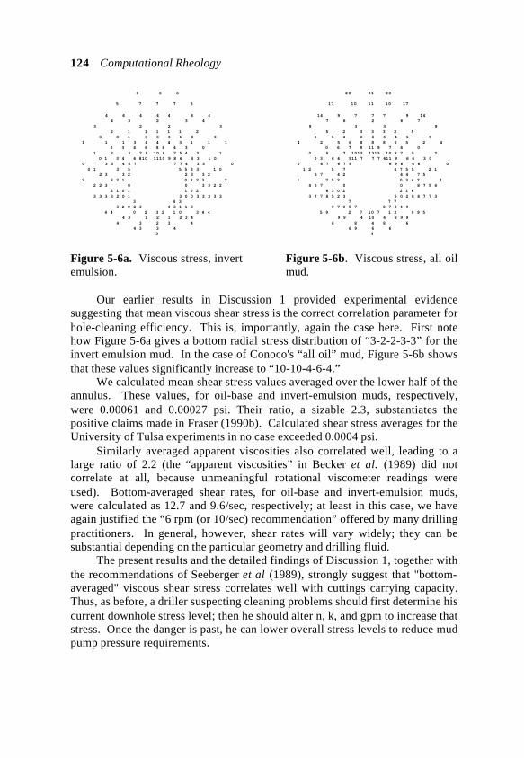
124 Computational Rheology
6 6 6
5 7 7 7 5
4 6 4 4 4 6 4 4 3 2 3 4 3 2 2 3 2 1 1 1 1 1 2 3 0 1 3 3 3 1 0 3 1 1 1 3 4 4 4 3 1 1 1 0 3 4 6 8 6 4 3 0 1 2 4 7 9 10 9 7 5 4 2 1 0 1 3 4 6 810 1110 9 8 6 4 3 1 0 0 3 3 4 4 7 7 7 4 3 3 0 0 1 3 5 5 5 3 3 1 0 2 3 3 2 2 3 3 2 2 3 2 1 0 2 2 3 2 2 2 3 0 0 3 3 2 2 2 1 0 1 1 0 2 3 3 3 3 2 0 1 3 0 0 3 3 3 3 3 3 4 3 3 2 0 2 3 4 3 1 1 3 4 4 0 2 3 2 1 0 3 4 4 4 3 1 2 1 2 3 4 4 3 2 3 4 4 3 3 4 3
Figure 5-6a. Viscous stress, invertemulsion.
20 21 20
17 10 11 10 17
14 9 7 7 7 9 14 7 6 2 6 7 9 3 3 9 5 2 3 3 3 2 5 5 1 4 6 6 6 4 1 5 4 2 5 6 8 8 8 6 5 2 4 0 6 7 9 11 9 7 6 0 2 5 7 1013 1313 10 8 7 5 2 0 3 6 6 911 7 7 7 611 9 6 6 3 0 0 6 7 6 7 9 6 9 6 6 6 0 1 2 5 7 4 7 5 5 2 1 5 7 4 2 4 4 7 5 1 7 5 2 0 3 4 7 1 4 5 7 0 0 8 7 5 4 6 3 0 2 2 1 6 3 7 7 8 5 2 3 5 0 2 8 8 7 7 3 7 7 7 9 7 0 5 7 8 7 3 4 9 5 9 2 7 10 7 1 2 9 9 5 9 9 4 10 4 8 9 9 6 8 4 8 6 6 9 6 6 4
Figure 5-6b. Viscous stress, all oilmud.
Our earlier results in Discussion 1 provided experimental evidencesuggesting that mean viscous shear stress is the correct correlation parameter forhole-cleaning efficiency. This is, importantly, again the case here. First notehow Figure 5-6a gives a bottom radial stress distribution of “3-2-2-3-3” for theinvert emulsion mud. In the case of Conoco's “all oil” mud, Figure 5-6b showsthat these values significantly increase to “10-10-4-6-4.”
We calculated mean shear stress values averaged over the lower half of theannulus. These values, for oil-base and invert-emulsion muds, respectively,were 0.00061 and 0.00027 psi. Their ratio, a sizable 2.3, substantiates thepositive claims made in Fraser (1990b). Calculated shear stress averages for theUniversity of Tulsa experiments in no case exceeded 0.0004 psi.
Similarly averaged apparent viscosities also correlated well, leading to alarge ratio of 2.2 (the “apparent viscosities” in Becker et al. (1989) did notcorrelate at all, because unmeaningful rotational viscometer readings wereused). Bottom-averaged shear rates, for oil-base and invert-emulsion muds,were calculated as 12.7 and 9.6/sec, respectively; at least in this case, we haveagain justified the “6 rpm (or 10/sec) recommendation” offered by many drillingpractitioners. In general, however, shear rates will vary widely; they can besubstantial depending on the particular geometry and drilling fluid.
The present results and the detailed findings of Discussion 1, together withthe recommendations of Seeberger et al (1989), strongly suggest that "bottom-averaged" viscous shear stress correlates well with cuttings carrying capacity.Thus, as before, a driller suspecting cleaning problems should first determine hiscurrent downhole stress level; then he should alter n, k, and gpm to increase thatstress. Once the danger is past, he can lower overall stress levels to reduce mudpump pressure requirements.
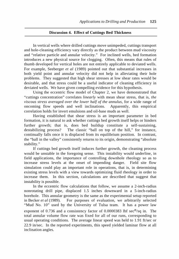
Applications to Drilling and Production 125
Discussion 4. Effect of Cuttings Bed Thickness
In vertical wells where drilled cuttings move unimpeded, cuttings transportand hole-cleaning efficiency vary directly as the product between mud viscosityand “relative particle and annular velocity.” For inclined wells, bed formationintroduces a new physical source for clogging. Often, this means that rules ofthumb developed for vertical holes are not entirely applicable to deviated wells.For example, Seeberger et al (1989) pointed out that substantial increases inboth yield point and annular velocity did not help in alleviating their holeproblems. They suggested that high shear stresses at low shear rates would bedesirable, and that stress could be a useful indicator of cleaning efficiency indeviated wells. We have given compelling evidence for this hypothesis.
Using the eccentric flow model of Chapter 2, we have demonstrated that“cuttings concentration” correlates linearly with mean shear stress, that is, theviscous stress averaged over the lower half of the annulus, for a wide range ofoncoming flow speeds and well inclinations. Apparently, this empiricalcorrelation holds for invert emulsions and oil-base muds as well.
Having established that shear stress is an important parameter in bedformation, it is natural to ask whether cuttings bed growth itself helps or hindersfurther growth; that is, does bed buildup constitute a self-sustaining,destabilizing process? The classic “ball on top of the hill,” for instance,continually falls once it is displaced from its equilibrium position. In contrast,the “ball in the valley” consistently returns to its origin, demonstrating “absolutestability.”
If cuttings bed growth itself induces further growth, the cleaning processwould be unstable in the foregoing sense. This instability would underline, infield applications, the importance of controlling downhole rheology so as toincrease stress levels at the onset of impending danger. Field site flowsimulation could play an important role in operations, that is, in determiningexisting stress levels with a view towards optimizing fluid rheology in order toincrease them. In this section, calculations are described that suggest thatinstability is possible.
In the eccentric flow calculations that follow, we assume a 2-inch-radiusnonrotating drill pipe, displaced 1.5 inches downward in a 5-inch-radiusborehole. This annular geometry is the same as the experimental setup reportedin Becker et al (1989). For purposes of evaluation, we arbitrarily selected“Mud No. 10” used by the University of Tulsa team. It has a power law
exponent of 0.736 and a consistency factor of 0.0000383 lbf secn/sq in. Thetotal annular volume flow rate was fixed for all of our runs, corresponding tousual operating conditions. The average linear speed was held to 1.91 ft/sec or22.9 in/sec. In the reported experiments, this speed yielded laminar flow at allinclination angles.
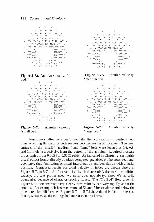
126 Computational Rheology
0 0 0 0 29 30 29 0
0 28 44 45 44 28 0 26 42 50 42 26 0 50 50 0 39 48 51 51 51 48 39 23 44 49 49 49 49 49 44 23 0 34 45 46 44 44 44 46 45 34 0 39 43 42 36 2636 42 43 39 19 40 38 2514 1414 253138 40 19 2933 3833 2213 0 0 0 01322 3338 3329 0 3332 271912 01227 3233 0 1523 28 10 0102328 2315 2627 15 0 815 2726 0 252213 6182225 0 111720 0 0 20201711 1917 9 0 51319 0 812141412 7 01012151412 8 0 2 0 2 1010 9 5 4 0 4 71010 0 5 7 4 4 4 6 7 8 5 0 3 5 5 5 5 7 5 3 0 4 4 4 0 0 2 2 0 0
Figure 5-7a. Annular velocity, “nobed.” 0 0 0
0 30 31 30 0
0 29 45 46 45 29 0 26 43 52 43 26 0 51 51 0 40 49 52 52 52 49 40 23 45 50 50 51 50 50 45 23 0 35 46 48 45 46 45 48 46 35 0 40 44 43 37 2737 43 44 40 19 41 39 2514 1414 253239 41 19 3034 3834 2313 0 0 0 01323 3438 3430 0 34 282012 01228 34 0 1523 3228 10 0102332 2315 2627 15 0 815 2726 0 252212 6172225 0 111719 0 0 191711 191512 0 4121819 0 6 0 6 0 710121210 2 0 2 8111210 7 6 5 1 1 6 6 4 2 3 2 4 7 6 5 4 3 3 3 4 5 0 0 3 0 0 1 0 0 0
Figure 5-7b. Annular velocity,“small bed.”
0 0 0
0 30 31 30 0
0 29 45 46 45 29 0 26 43 52 43 26 0 51 51 0 40 49 52 52 52 49 40 23 45 50 50 51 50 50 45 23 0 35 46 48 45 46 45 48 46 35 0 40 44 43 37 2737 43 44 40 19 41 39 2514 1414 253239 41 19 3034 3934 2313 0 0 0 01323 3439 3430 0 34 282012 01228 34 0 1523 3228 10 0102332 2315 2727 15 0 815 2727 0 252212 6182225 0 111720 0 0 201711 2015 9 0 5131920 0 9 6 0 9 0
711131311 2 0 2 131311 7 8 4 2 1 2 7 8 6 4 3 1 1 1 1 4 4 8 6 0 0 0 1 0 0 2 0 4 0
Figure 5-7c. Annular velocity,“medium bed.”
0 0 0
0 30 31 30 0
0 29 45 46 45 29 0 26 43 52 43 26 0 51 51 0 40 49 52 52 52 49 40 23 45 50 50 51 50 50 45 23 0 35 46 48 45 46 45 48 46 35 0 40 44 43 37 2737 43 44 40 19 41 39 2514 1414 253239 41 19
3034 3934 2313 0 0 0 01323 3439 3430 0 34 282012 01228 34 0 1524 3228 10 0102332 2415 2727 15 0 815 2727 0 262213 6182226 0 11182020 0 0 20201811 1917 9 0 51319 0 8 11 6 0 911 8 0 121414 3 0 3 13141412 9 8 2 0 2 5 9 5 8 9 3 3 2 0 0 0 0 3 3 8 5 0 0 0 0 0 0 2 0 0
Figure 5-7d. Annular velocity,“large bed.”
Four case studies were performed, the first containing no cuttings bed;then, assuming flat cuttings beds successively increasing in thickness. The levelsurfaces of the “small,” “medium,” and “large” beds were located at 0.4, 0.8,and 1.0 inch, respectively, from the bottom of the annulus. Required pressuredrops varied from 0.0054 to 0.0055 psi/ft. As indicated in Chapter 2, the highlyvisual output format directly overlays computed quantities on the cross-sectionalgeometry, thus facilitating physical interpretation and correlation with annularposition. Computed results for axial velocity in in/sec are shown above inFigures 5-7a to 5-7d. All four velocity distributions satisfy the no-slip conditionexactly; the text plotter used, we note, does not always show 0’s at solidboundaries because of character spacing issues. The “No Bed” flow given inFigure 5-7a demonstrates very clearly how velocity can vary rapidly about theannulus. For example, it has maximums of 51 and 5 in/sec above and below thepipe, a ten-fold difference. Figures 5-7b to 5-7d show that this factor increases,that is, worsens, as the cuttings bed increases in thickness.

Applications to Drilling and Production 127 55 57 55
49 45 47 45 49
39 39 28 29 28 39 39 30 24 13 24 30 27 12 12 27 17 9 4 4 4 9 17 19 4 6 18 18 18 6 4 19 12 8 9 19 31 31 31 19 9 8 12 1 19 30 44 5844 30 19 1
6 12 28 5169 7269 513628 12 6 0 8 1924 436280 8380706243 2419 8 0 1 1519 293250 555029 1915 1 5 9 20 35 37352020 9 5 1315 2018 1920 1513 14 1514 8 4111415 14 151517 1 1 15171515 13 8 212 7 313 23222018 9 210 21 3 21418202223 21 2621 1511 21518 2918 9 415 2725 0 15 1815 6 0 212527 2419 5 8 5 141924 28 15 13 15 28 2622 20 26 24
Figure 5-8a. Viscous stress, “nobed.”
56 58 56
50 46 48 46 50
40 40 29 30 29 40 40 31 24 14 24 31 27 13 13 27 17 9 5 4 5 9 17 19 4 6 18 18 18 6 4 19 13 8 9 19 31 32 31 19 9 8 13 2 20 30 45 5945 30 20 2 6 13 28 5271 7371 523628 13 6 1 9 2025 446381 8581716344 2520 9 1 1 15 293351 565129 15 1 611 1920 35 37352119 11 6 1518 2018 1920 1815 17 1715 8 4111517 17 181919 0 0 191918 17 8 212 7 21317 29 10 2110 29 26221814 1 20 2520 4 7182226 3 922 22 3 14 012 912 0 314 17 1110 810 11 17 20251523 21192325 20
Figure 5-8b. Viscous stress,“small bed.”
56 58 56
50 46 48 46 50
40 40 29 30 29 40 40 31 24 14 24 31 27 13 13 27 17 9 5 4 5 9 17 19 4 6 18 18 18 6 4 19 13 8 9 19 31 32 31 19 9 8 13 2 20 30 45 5945 30 20 2 6 13 28 5271 7371 523628 13 6 1 8 2025 446381 8581716344 2520 8 1 1 15 293351 565129 15 1 510 1920 35 37352119 10 5 1417 2018 1920 1714 15 1714 8 4111417 15 171818 1 1 181817 17 8 212 7 31317 27 410 21 4 27 25211814 2 20 2520 8142125 41414 1814 2 4 19 14 3 0 4 5 0 8141019 25 30 2013 6 20 26302225
Figure 5-8c. Viscous stress,“medium bed.”
56 58 56
50 46 48 46 50
40 40 29 30 29 40 40 31 24 14 24 31 27 13 13 27 17 9 5 4 5 9 17 19 4 6 18 18 18 6 4 19 13 8 9 19 31 32 31 19 9 8 13 2 20 30 45 5945 30 20 2 6 12 28 5271 7371 523628 12 6
1 8 2025 446381 8581716344 2520 8 1 1 15 293351 565129 15 1 510 1920 35 37352119 10 5 1417 2018 1920 1714 14 1714 8 4111417 14 15171717 1 1 17171715 13 8 212 7 313 2423 210 21 3 2 2324 211814 13 2413 8141821 10 4 7 15 7 810 2521152115 1 7 5 3 7 921 2125 28 32 1711 5 17 2732 28
Figure 5-8d. Viscous stress, “largebed.”
Figures 5-8a to 5-8d give computed results for the vertical component ofthe shear stress, that is, “apparent viscosity (x,y) × strain rate dU/dx,” where xincreases downward. Results for the stress related to “dU/dy,” not shownbecause of space limitations, behaved similarly. For clarity, only the absolutevalues are displayed; the actual values, which are separately available in
tabulated form, vary from O(10-4) to O(10-3) psi.Note how the bottom viscous stresses decrease in magnitude as the cuttings
bed builds in thickness. This decrease, which is accompanied by decreases inthroughput area, further compounds cuttings transport problems and decreasescleaning efficiency. Thus, hole clogging is a self-sustaining, destabilizingprocess. Unless the mud rheology itself is changed in the direction of increasingstress, differential sticking and stuck pipe are possible. This decrease of viscousstress with increasing bed thickness is also supported experimentally. Quigley
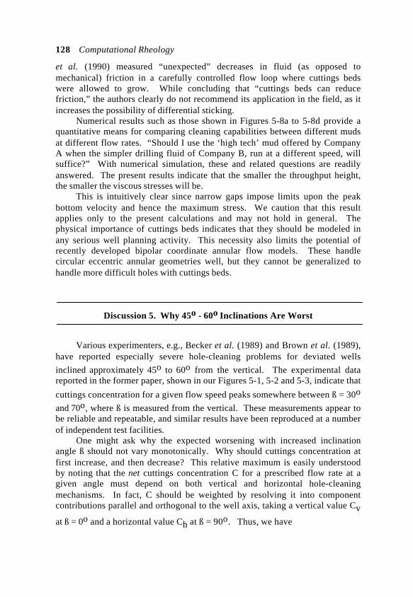
128 Computational Rheology
et al. (1990) measured “unexpected” decreases in fluid (as opposed tomechanical) friction in a carefully controlled flow loop where cuttings bedswere allowed to grow. While concluding that “cuttings beds can reducefriction,” the authors clearly do not recommend its application in the field, as itincreases the possibility of differential sticking.
Numerical results such as those shown in Figures 5-8a to 5-8d provide aquantitative means for comparing cleaning capabilities between different mudsat different flow rates. “Should I use the ‘high tech’ mud offered by CompanyA when the simpler drilling fluid of Company B, run at a different speed, willsuffice?” With numerical simulation, these and related questions are readilyanswered. The present results indicate that the smaller the throughput height,the smaller the viscous stresses will be.
This is intuitively clear since narrow gaps impose limits upon the peakbottom velocity and hence the maximum stress. We caution that this resultapplies only to the present calculations and may not hold in general. Thephysical importance of cuttings beds indicates that they should be modeled inany serious well planning activity. This necessity also limits the potential ofrecently developed bipolar coordinate annular flow models. These handlecircular eccentric annular geometries well, but they cannot be generalized tohandle more difficult holes with cuttings beds.
Discussion 5. Why 45o - 60o Inclinations Are Worst
Various experimenters, e.g., Becker et al. (1989) and Brown et al. (1989),have reported especially severe hole-cleaning problems for deviated wells
inclined approximately 45o to 60o from the vertical. The experimental datareported in the former paper, shown in our Figures 5-1, 5-2 and 5-3, indicate that
cuttings concentration for a given flow speed peaks somewhere between ß = 30o
and 70o, where ß is measured from the vertical. These measurements appear tobe reliable and repeatable, and similar results have been reproduced at a numberof independent test facilities.
One might ask why the expected worsening with increased inclinationangle ß should not vary monotonically. Why should cuttings concentration atfirst increase, and then decrease? This relative maximum is easily understoodby noting that the net cuttings concentration C for a prescribed flow rate at agiven angle must depend on both vertical and horizontal hole-cleaningmechanisms. In fact, C should be weighted by resolving it into componentcontributions parallel and orthogonal to the well axis, taking a vertical value Cv
at ß = 0o and a horizontal value Ch at ß = 90o. Thus, we have
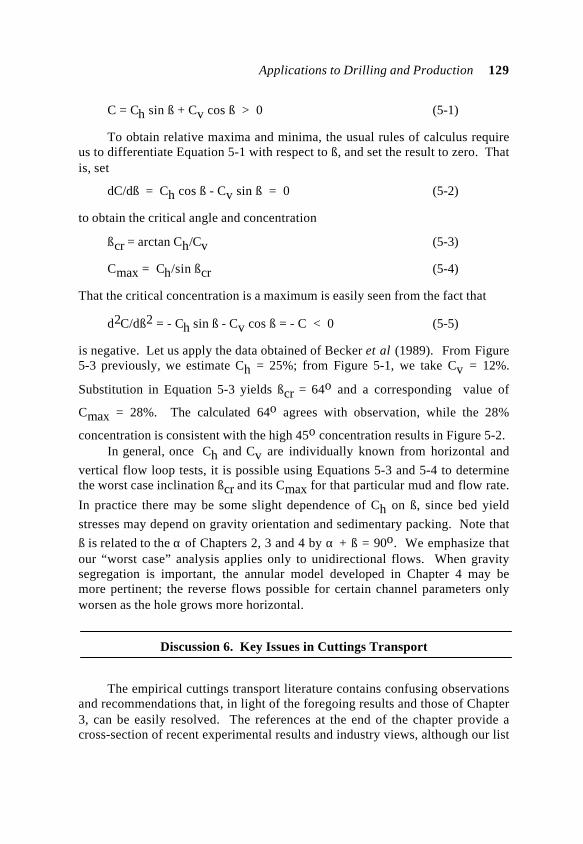
Applications to Drilling and Production 129
C = Ch sin ß + Cv cos ß > 0 (5-1)
To obtain relative maxima and minima, the usual rules of calculus requireus to differentiate Equation 5-1 with respect to ß, and set the result to zero. Thatis, set
dC/dß = Ch cos ß - Cv sin ß = 0 (5-2)
to obtain the critical angle and concentration
ßcr = arctan Ch/Cv (5-3)
Cmax = Ch/sin ßcr (5-4)
That the critical concentration is a maximum is easily seen from the fact that
d2C/dß2 = - Ch sin ß - Cv cos ß = - C < 0 (5-5)
is negative. Let us apply the data obtained of Becker et al (1989). From Figure5-3 previously, we estimate Ch = 25%; from Figure 5-1, we take Cv = 12%.
Substitution in Equation 5-3 yields ßcr = 64o and a corresponding value of
Cmax = 28%. The calculated 64o agrees with observation, while the 28%
concentration is consistent with the high 45o concentration results in Figure 5-2.In general, once Ch and Cv are individually known from horizontal and
vertical flow loop tests, it is possible using Equations 5-3 and 5-4 to determinethe worst case inclination ßcr and its Cmax for that particular mud and flow rate.
In practice there may be some slight dependence of Ch on ß, since bed yield
stresses may depend on gravity orientation and sedimentary packing. Note that
ß is related to the α of Chapters 2, 3 and 4 by α + ß = 90o. We emphasize thatour “worst case” analysis applies only to unidirectional flows. When gravitysegregation is important, the annular model developed in Chapter 4 may bemore pertinent; the reverse flows possible for certain channel parameters onlyworsen as the hole grows more horizontal.
Discussion 6. Key Issues in Cuttings Transport
The empirical cuttings transport literature contains confusing observationsand recommendations that, in light of the foregoing results and those of Chapter3, can be easily resolved. The references at the end of the chapter provide across-section of recent experimental results and industry views, although our list
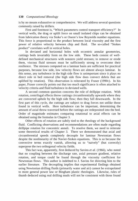
130 Computational Rheology
is by no means exhaustive or comprehensive. We will address several questionscommonly raised by drillers.
First and foremost is, “Which parameters control transport efficiency?” Invertical wells, the drag or uplift force on small isolated chips can be obtainedfrom lubrication theory via Stoke’s or Oseen’s low Reynolds number equations.This force is proportional to the product between local viscosity and the firstpower of relative velocity between chip and fluid. The so-called “Stokesproduct” correlates well in vertical holes.
In deviated and horizontal holes with eccentric annular geometries,cuttings beds invariably form on the low side. These beds consist of well-defined mechanical structures with nonzero yield stresses; to remove or erodethem, viscous fluid stresses must be sufficiently strong to overcome theirresilience. The stresses computed on a laminar basis are sufficient for practicalpurposes, because low side, low velocity flows are almost always laminar. Inthis sense, any turbulence in the high side flow is unimportant since it plays nodirect role in bed removal (the high side flow does convect debris that areuplifted by rotation). This observation is reiterated by Fraser (1990c). In hispaper, Fraser correctly points out that too much significance is often attached tovelocity criteria and fluid turbulence in deviated wells.
A second common question concerns the role of drillpipe rotation. Withrotation, centrifugal effects throw cuttings circumferentially upwards where theyare convected uphole by the high side flow; then they fall downwards. In thefirst part of this cycle, the cuttings are subject to drag forces not unlike thosefound in vertical wells. Here turbulence can be important, determining theamount of axial throw traversed before the cuttings are redeposited into the bed.Order of magnitude estimates comparing rotational to axial effects can beobtained using the formulas in Chapter 3.
Other effects of rotation are subtly tied to the rheology of the backgroundfluid. Conflicting observations and recommendations are often made regardingdrillpipe rotation for concentric annuli. To resolve them, we need to reiteratesome theoretical results of Chapter 3. There we demonstrated that axial andcircumferential speeds completely decouple for laminar Newtonian flowsdespite the nonlinearity of the Navier-Stokes equations. This is so because theconvective terms exactly vanish, allowing us to “naively” (but correctly)superpose the two orthogonal velocity fields.
This fact was, apparently, first deduced by Savins et al. (1966), who notedthat no coupling between the discharge rate, axial pressure gradient, relativerotation, and torque could be found through the viscosity coefficient forNewtonian flows. This author is indebted to J. Savins for directing him to theearlier literature. The decoupling implies that experimental findings obtainedusing Newtonian drilling fluids (primarily water and air) cannot be extrapolatedto more general power law or Bingham plastic rheologies. Likewise, rules ofthumb deduced using real drilling muds will not be consistent with those found
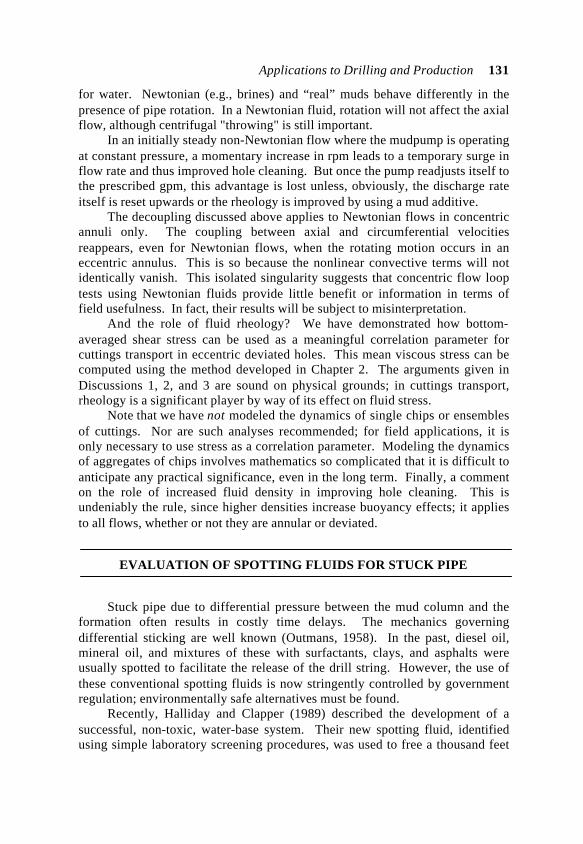
Applications to Drilling and Production 131
for water. Newtonian (e.g., brines) and “real” muds behave differently in thepresence of pipe rotation. In a Newtonian fluid, rotation will not affect the axialflow, although centrifugal "throwing" is still important.
In an initially steady non-Newtonian flow where the mudpump is operatingat constant pressure, a momentary increase in rpm leads to a temporary surge inflow rate and thus improved hole cleaning. But once the pump readjusts itself tothe prescribed gpm, this advantage is lost unless, obviously, the discharge rateitself is reset upwards or the rheology is improved by using a mud additive.
The decoupling discussed above applies to Newtonian flows in concentricannuli only. The coupling between axial and circumferential velocitiesreappears, even for Newtonian flows, when the rotating motion occurs in aneccentric annulus. This is so because the nonlinear convective terms will notidentically vanish. This isolated singularity suggests that concentric flow looptests using Newtonian fluids provide little benefit or information in terms offield usefulness. In fact, their results will be subject to misinterpretation.
And the role of fluid rheology? We have demonstrated how bottom-averaged shear stress can be used as a meaningful correlation parameter forcuttings transport in eccentric deviated holes. This mean viscous stress can becomputed using the method developed in Chapter 2. The arguments given inDiscussions 1, 2, and 3 are sound on physical grounds; in cuttings transport,rheology is a significant player by way of its effect on fluid stress.
Note that we have not modeled the dynamics of single chips or ensemblesof cuttings. Nor are such analyses recommended; for field applications, it isonly necessary to use stress as a correlation parameter. Modeling the dynamicsof aggregates of chips involves mathematics so complicated that it is difficult toanticipate any practical significance, even in the long term. Finally, a commenton the role of increased fluid density in improving hole cleaning. This isundeniably the rule, since higher densities increase buoyancy effects; it appliesto all flows, whether or not they are annular or deviated.
EVALUATION OF SPOTTING FLUIDS FOR STUCK PIPE
Stuck pipe due to differential pressure between the mud column and theformation often results in costly time delays. The mechanics governingdifferential sticking are well known (Outmans, 1958). In the past, diesel oil,mineral oil, and mixtures of these with surfactants, clays, and asphalts wereusually spotted to facilitate the release of the drill string. However, the use ofthese conventional spotting fluids is now stringently controlled by governmentregulation; environmentally safe alternatives must be found.
Recently, Halliday and Clapper (1989) described the development of asuccessful, non-toxic, water-base system. Their new spotting fluid, identifiedusing simple laboratory screening procedures, was used to free a thousand feet
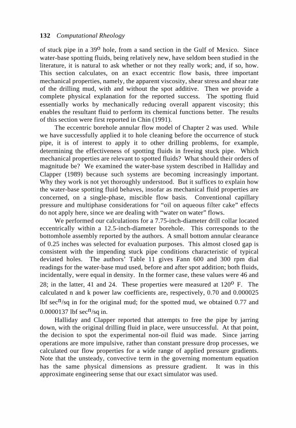
132 Computational Rheology
of stuck pipe in a 39o hole, from a sand section in the Gulf of Mexico. Sincewater-base spotting fluids, being relatively new, have seldom been studied in theliterature, it is natural to ask whether or not they really work; and, if so, how.This section calculates, on an exact eccentric flow basis, three importantmechanical properties, namely, the apparent viscosity, shear stress and shear rateof the drilling mud, with and without the spot additive. Then we provide acomplete physical explanation for the reported success. The spotting fluidessentially works by mechanically reducing overall apparent viscosity; thisenables the resultant fluid to perform its chemical functions better. The resultsof this section were first reported in Chin (1991).
The eccentric borehole annular flow model of Chapter 2 was used. Whilewe have successfully applied it to hole cleaning before the occurrence of stuckpipe, it is of interest to apply it to other drilling problems, for example,determining the effectiveness of spotting fluids in freeing stuck pipe. Whichmechanical properties are relevant to spotted fluids? What should their orders ofmagnitude be? We examined the water-base system described in Halliday andClapper (1989) because such systems are becoming increasingly important.Why they work is not yet thoroughly understood. But it suffices to explain howthe water-base spotting fluid behaves, insofar as mechanical fluid properties areconcerned, on a single-phase, miscible flow basis. Conventional capillarypressure and multiphase considerations for “oil on aqueous filter cake” effectsdo not apply here, since we are dealing with “water on water” flows.
We performed our calculations for a 7.75-inch-diameter drill collar locatedeccentrically within a 12.5-inch-diameter borehole. This corresponds to thebottomhole assembly reported by the authors. A small bottom annular clearanceof 0.25 inches was selected for evaluation purposes. This almost closed gap isconsistent with the impending stuck pipe conditions characteristic of typicaldeviated holes. The authors’ Table 11 gives Fann 600 and 300 rpm dialreadings for the water-base mud used, before and after spot addition; both fluids,incidentally, were equal in density. In the former case, these values were 46 and
28; in the latter, 41 and 24. These properties were measured at 120o F. Thecalculated n and k power law coefficients are, respectively, 0.70 and 0.000025
lbf secn/sq in for the original mud; for the spotted mud, we obtained 0.77 and
0.0000137 lbf secn/sq in.Halliday and Clapper reported that attempts to free the pipe by jarring
down, with the original drilling fluid in place, were unsuccessful. At that point,the decision to spot the experimental non-oil fluid was made. Since jarringoperations are more impulsive, rather than constant pressure drop processes, wecalculated our flow properties for a wide range of applied pressure gradients.Note that the unsteady, convective term in the governing momentum equationhas the same physical dimensions as pressure gradient. It was in thisapproximate engineering sense that our exact simulator was used.
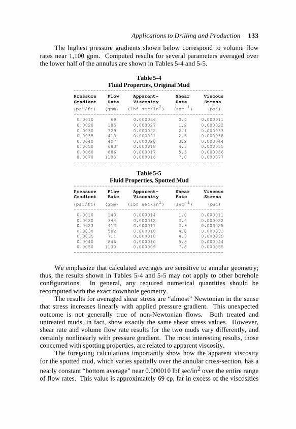
Applications to Drilling and Production 133
The highest pressure gradients shown below correspond to volume flowrates near 1,100 gpm. Computed results for several parameters averaged overthe lower half of the annulus are shown in Tables 5-4 and 5-5.
Table 5-4Fluid Properties, Original Mud
----------------------------------------------------- Pressure Flow Apparent- Shear Viscous Gradient Rate Viscosity Rate Stress
(psi/ft) (gpm) (lbf sec/in2) (sec-1) (psi) ----------------------------------------------------- 0.0010 69 0.000036 0.4 0.000011 0.0020 185 0.000027 1.2 0.000022 0.0030 329 0.000022 2.1 0.000033 0.0035 410 0.000021 2.6 0.000038 0.0040 497 0.000020 3.2 0.000044 0.0050 683 0.000018 4.3 0.000055 0.0060 886 0.000017 5.6 0.000066 0.0070 1105 0.000016 7.0 0.000077 -----------------------------------------------------
Table 5-5Fluid Properties, Spotted Mud
----------------------------------------------------- Pressure Flow Apparent- Shear Viscous Gradient Rate Viscosity Rate Stress
(psi/ft) (gpm) (lbf sec/in2) (sec-1) (psi) ----------------------------------------------------- 0.0010 140 0.000014 1.0 0.000011 0.0020 344 0.000012 2.4 0.000022 0.0023 412 0.000011 2.8 0.000025 0.0030 582 0.000010 4.0 0.000033 0.0035 711 0.000010 4.9 0.000039 0.0040 846 0.000010 5.8 0.000044 0.0050 1130 0.000009 7.8 0.000055 -----------------------------------------------------
We emphasize that calculated averages are sensitive to annular geometry;thus, the results shown in Tables 5-4 and 5-5 may not apply to other boreholeconfigurations. In general, any required numerical quantities should berecomputed with the exact downhole geometry.
The results for averaged shear stress are “almost” Newtonian in the sensethat stress increases linearly with applied pressure gradient. This unexpectedoutcome is not generally true of non-Newtonian flows. Both treated anduntreated muds, in fact, show exactly the same shear stress values. However,shear rate and volume flow rate results for the two muds vary differently, andcertainly nonlinearly with pressure gradient. The most interesting results, thoseconcerned with spotting properties, are related to apparent viscosity.
The foregoing calculations importantly show how the apparent viscosityfor the spotted mud, which varies spatially over the annular cross-section, has a
nearly constant “bottom average” near 0.000010 lbf sec/in2 over the entire rangeof flow rates. This value is approximately 69 cp, far in excess of the viscosities
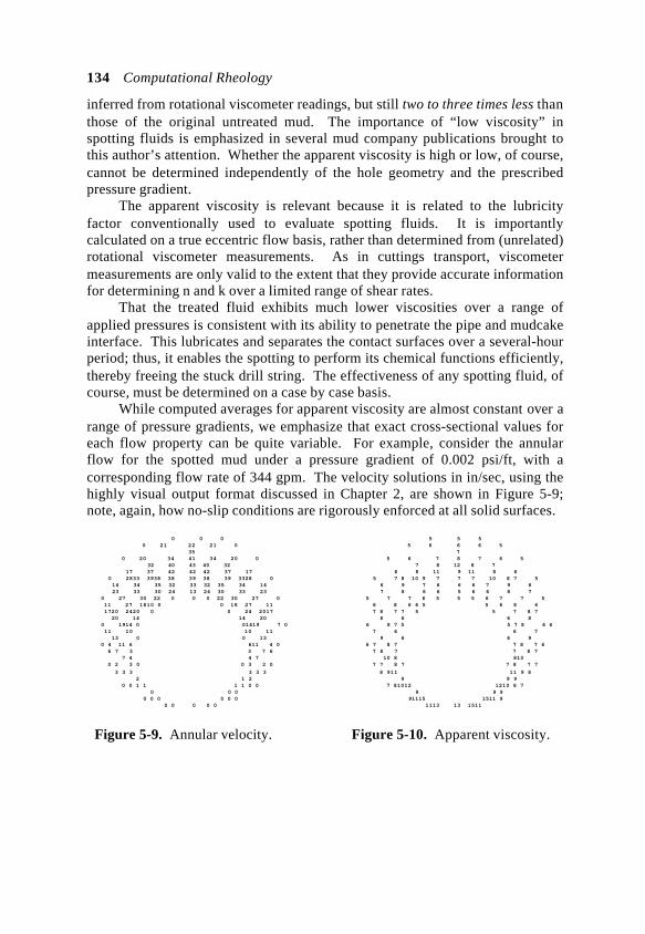
134 Computational Rheology
inferred from rotational viscometer readings, but still two to three times less thanthose of the original untreated mud. The importance of “low viscosity” inspotting fluids is emphasized in several mud company publications brought tothis author’s attention. Whether the apparent viscosity is high or low, of course,cannot be determined independently of the hole geometry and the prescribedpressure gradient.
The apparent viscosity is relevant because it is related to the lubricityfactor conventionally used to evaluate spotting fluids. It is importantlycalculated on a true eccentric flow basis, rather than determined from (unrelated)rotational viscometer measurements. As in cuttings transport, viscometermeasurements are only valid to the extent that they provide accurate informationfor determining n and k over a limited range of shear rates.
That the treated fluid exhibits much lower viscosities over a range ofapplied pressures is consistent with its ability to penetrate the pipe and mudcakeinterface. This lubricates and separates the contact surfaces over a several-hourperiod; thus, it enables the spotting to perform its chemical functions efficiently,thereby freeing the stuck drill string. The effectiveness of any spotting fluid, ofcourse, must be determined on a case by case basis.
While computed averages for apparent viscosity are almost constant over arange of pressure gradients, we emphasize that exact cross-sectional values foreach flow property can be quite variable. For example, consider the annularflow for the spotted mud under a pressure gradient of 0.002 psi/ft, with acorresponding flow rate of 344 gpm. The velocity solutions in in/sec, using thehighly visual output format discussed in Chapter 2, are shown in Figure 5-9;note, again, how no-slip conditions are rigorously enforced at all solid surfaces.
0 0 0 0 21 22 21 0 35 0 20 34 41 34 20 0 32 40 43 40 32 17 37 42 42 42 37 17 0 2833 3938 38 39 38 39 3328 0 14 34 35 32 33 32 35 34 14 23 33 30 24 13 24 30 33 23 0 27 30 22 0 0 0 22 30 27 0 11 27 1810 0 0 18 27 11 1720 2420 0 0 24 2017 20 14 14 20 0 1914 0 01419 7 0 11 10 10 11 13 0 0 13 0 4 11 6 611 4 0 6 7 3 3 7 6 7 4 4 7 0 2 3 0 0 3 2 0
3 3 3 3 3 3 2 1 2 0 0 1 1 1 1 0 0 0 0 0 0 0 0 0 0 0 0 0 0 0 0
Figure 5-9. Annular velocity.
5 5 5 5 6 6 6 5 7 5 6 7 8 7 6 5 7 8 12 8 7 6 8 11 9 11 8 6 5 7 8 10 9 7 7 7 10 8 7 5 6 9 7 6 6 6 7 9 6 7 8 6 6 5 6 6 8 7 5 7 7 6 5 5 5 6 7 7 5 6 8 6 6 5 5 6 8 6 7 8 7 7 5 5 7 8 7 8 6 6 8 6 8 7 5 5 7 8 6 6 7 6 6 7 9 6 6 9 6 7 8 7 7 8 7 6 7 8 7 7 8 7 10 8 810 7 7 8 7 7 8 7 7
8 911 11 9 8 9 9 9 7 81012 1210 8 7 9 9 9 91115 1511 9 1113 13 1511
Figure 5-10. Apparent viscosity.
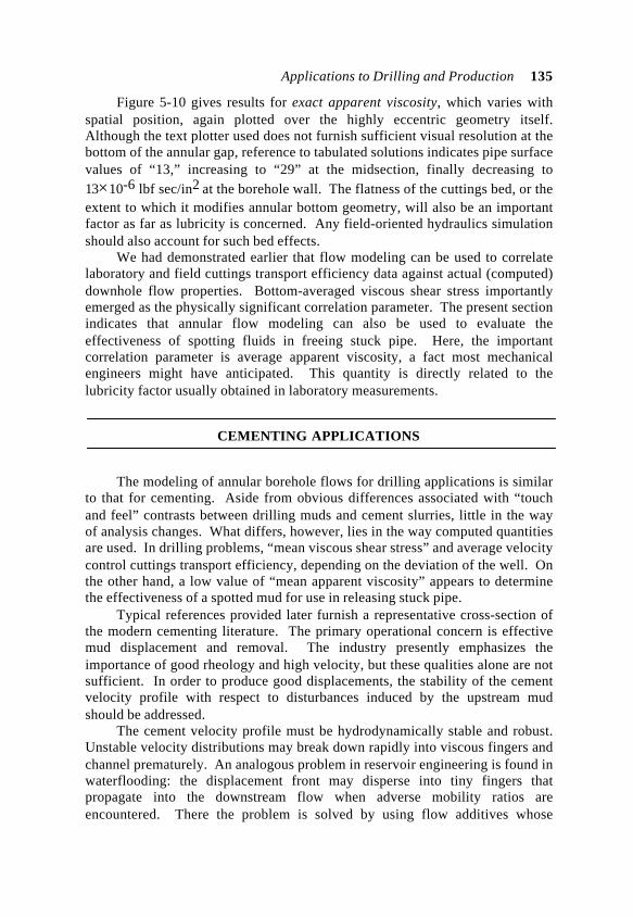
Applications to Drilling and Production 135
Figure 5-10 gives results for exact apparent viscosity, which varies withspatial position, again plotted over the highly eccentric geometry itself.Although the text plotter used does not furnish sufficient visual resolution at thebottom of the annular gap, reference to tabulated solutions indicates pipe surfacevalues of “13,” increasing to “29” at the midsection, finally decreasing to13×10-6 lbf sec/in2 at the borehole wall. The flatness of the cuttings bed, or theextent to which it modifies annular bottom geometry, will also be an importantfactor as far as lubricity is concerned. Any field-oriented hydraulics simulationshould also account for such bed effects.
We had demonstrated earlier that flow modeling can be used to correlatelaboratory and field cuttings transport efficiency data against actual (computed)downhole flow properties. Bottom-averaged viscous shear stress importantlyemerged as the physically significant correlation parameter. The present sectionindicates that annular flow modeling can also be used to evaluate theeffectiveness of spotting fluids in freeing stuck pipe. Here, the importantcorrelation parameter is average apparent viscosity, a fact most mechanicalengineers might have anticipated. This quantity is directly related to thelubricity factor usually obtained in laboratory measurements.
CEMENTING APPLICATIONS
The modeling of annular borehole flows for drilling applications is similarto that for cementing. Aside from obvious differences associated with “touchand feel” contrasts between drilling muds and cement slurries, little in the wayof analysis changes. What differs, however, lies in the way computed quantitiesare used. In drilling problems, “mean viscous shear stress” and average velocitycontrol cuttings transport efficiency, depending on the deviation of the well. Onthe other hand, a low value of “mean apparent viscosity” appears to determinethe effectiveness of a spotted mud for use in releasing stuck pipe.
Typical references provided later furnish a representative cross-section ofthe modern cementing literature. The primary operational concern is effectivemud displacement and removal. The industry presently emphasizes theimportance of good rheology and high velocity, but these qualities alone are notsufficient. In order to produce good displacements, the stability of the cementvelocity profile with respect to disturbances induced by the upstream mudshould be addressed.
The cement velocity profile must be hydrodynamically stable and robust.Unstable velocity distributions may break down rapidly into viscous fingers andchannel prematurely. An analogous problem in reservoir engineering is found inwaterflooding: the displacement front may disperse into tiny fingers thatpropagate into the downstream flow when adverse mobility ratios areencountered. There the problem is solved by using flow additives whose
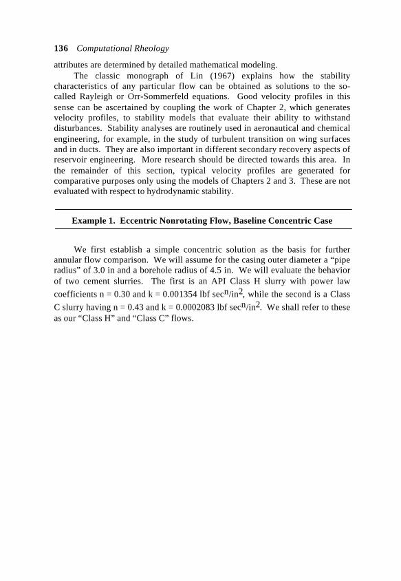
136 Computational Rheology
attributes are determined by detailed mathematical modeling.The classic monograph of Lin (1967) explains how the stability
characteristics of any particular flow can be obtained as solutions to the so-called Rayleigh or Orr-Sommerfeld equations. Good velocity profiles in thissense can be ascertained by coupling the work of Chapter 2, which generatesvelocity profiles, to stability models that evaluate their ability to withstanddisturbances. Stability analyses are routinely used in aeronautical and chemicalengineering, for example, in the study of turbulent transition on wing surfacesand in ducts. They are also important in different secondary recovery aspects ofreservoir engineering. More research should be directed towards this area. Inthe remainder of this section, typical velocity profiles are generated forcomparative purposes only using the models of Chapters 2 and 3. These are notevaluated with respect to hydrodynamic stability.
Example 1. Eccentric Nonrotating Flow, Baseline Concentric Case
We first establish a simple concentric solution as the basis for furtherannular flow comparison. We will assume for the casing outer diameter a “piperadius” of 3.0 in and a borehole radius of 4.5 in. We will evaluate the behaviorof two cement slurries. The first is an API Class H slurry with power law
coefficients n = 0.30 and k = 0.001354 lbf secn/in2, while the second is a Class
C slurry having n = 0.43 and k = 0.0002083 lbf secn/in2. We shall refer to theseas our “Class H” and “Class C” flows.
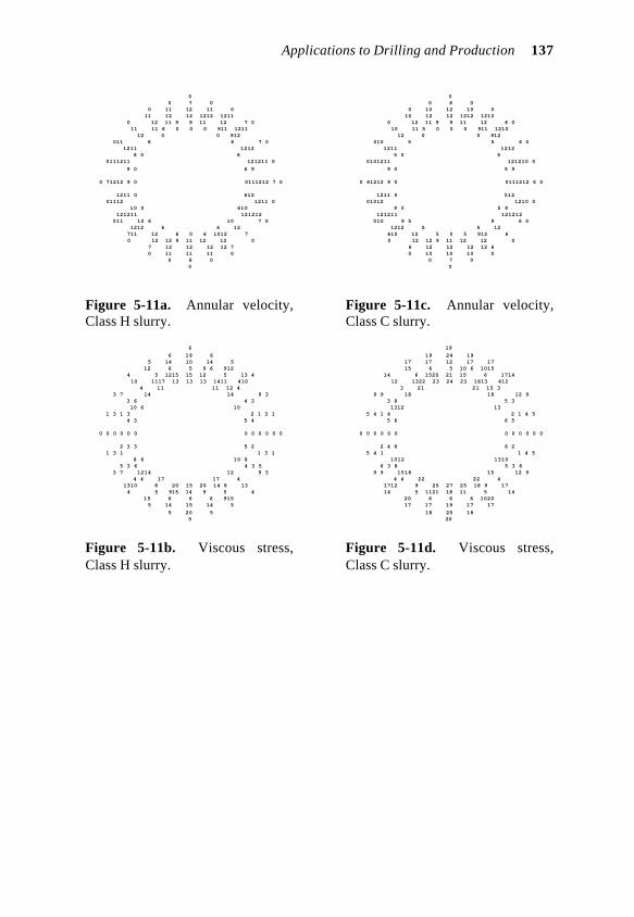
Applications to Drilling and Production 137
0 0 7 0 0 11 12 11 0 11 12 12 1212 1211 0 12 11 9 9 11 12 7 0 11 11 6 0 0 0 911 1211 12 0 0 912 011 6 6 7 0 1211 1212 6 0 6 0111211 121211 0
9 0 6 9
0 71212 9 0 0111212 7 0
1211 0 612 01112 1211 0 10 0 610 121211 121212 011 10 6 10 7 0 1212 6 6 12 711 12 6 0 6 1012 7 0 12 12 9 11 12 12 0 7 12 12 12 12 7 0 11 11 11 0 0 8 0 0
Figure 5-11a. Annular velocity,Class H slurry.
6
6 19 6 5 14 10 14 5 12 6 5 9 6 912 4 5 1215 15 12 5 13 4 10 1117 13 13 13 1411 410 4 11 11 12 4 3 7 14 14 9 3 3 6 4 3 10 6 10 1 3 1 3 2 1 3 1 4 3 5 4
0 0 0 0 0 0 0 0 0 0 0 0
2 3 3 5 2 1 3 1 1 3 1 8 6 10 8 5 3 6 4 3 5 3 7 1214 12 9 3 4 4 17 17 4 1310 8 20 15 20 14 8 13 4 5 915 14 9 5 4 15 6 6 6 915 5 14 15 14 5
5 20 5 5
Figure 5-11b. Viscous stress,Class H slurry.
0 0 6 0 0 10 12 10 0 10 12 12 1212 1210 0 12 11 9 9 11 12 6 0 10 11 5 0 0 0 911 1210 12 0 0 912 010 5 5 6 0 1211 1212 5 0 5 0101211 121210 0
9 0 5 9
0 61212 9 0 0111212 6 0
1211 0 512 01012 1210 0 9 0 5 9 121211 121212 010 9 5 9 6 0 1212 5 5 12 610 12 5 0 5 912 6 0 12 12 9 11 12 12 0 6 12 12 12 12 6 0 10 10 10 0 0 7 0 0
Figure 5-11c. Annular velocity,Class C slurry.
19
19 24 19 17 17 12 17 17 15 6 5 10 6 1015 14 6 1520 21 15 6 1714 12 1322 23 24 23 1813 412 3 21 21 15 3 9 9 18 18 12 9 3 8 5 3 1312 13 5 4 1 4 2 1 4 5 5 6 6 5
0 0 0 0 0 0 0 0 0 0 0 0
2 4 6 6 2 5 4 1 1 4 5 1012 1310 6 3 8 5 3 6 9 9 1518 15 12 9 4 4 22 22 4 1712 9 25 27 25 18 9 17 14 5 1121 18 11 5 14 20 6 6 6 1020 17 17 19 17 17
18 25 18 20
Figure 5-11d. Viscous stress,Class C slurry.
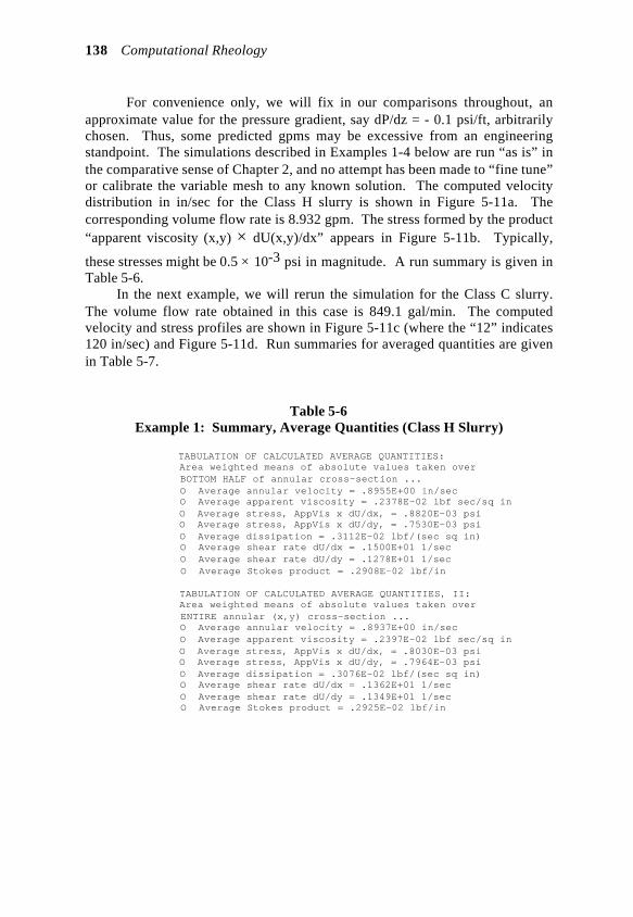
138 Computational Rheology
For convenience only, we will fix in our comparisons throughout, anapproximate value for the pressure gradient, say dP/dz = - 0.1 psi/ft, arbitrarilychosen. Thus, some predicted gpms may be excessive from an engineeringstandpoint. The simulations described in Examples 1-4 below are run “as is” inthe comparative sense of Chapter 2, and no attempt has been made to “fine tune”or calibrate the variable mesh to any known solution. The computed velocitydistribution in in/sec for the Class H slurry is shown in Figure 5-11a. Thecorresponding volume flow rate is 8.932 gpm. The stress formed by the product“apparent viscosity (x,y) × dU(x,y)/dx” appears in Figure 5-11b. Typically,
these stresses might be 0.5 × 10⁻³ psi in magnitude. A run summary is given inTable 5-6.
In the next example, we will rerun the simulation for the Class C slurry.The volume flow rate obtained in this case is 849.1 gal/min. The computedvelocity and stress profiles are shown in Figure 5-11c (where the “12” indicates120 in/sec) and Figure 5-11d. Run summaries for averaged quantities are givenin Table 5-7.
Table 5-6Example 1: Summary, Average Quantities (Class H Slurry)
TABULATION OF CALCULATED AVERAGE QUANTITIES: Area weighted means of absolute values taken over BOTTOM HALF of annular cross-section ... O Average annular velocity = .8955E+00 in/sec O Average apparent viscosity = .2378E-02 lbf sec/sq in O Average stress, AppVis x dU/dx, = .8820E-03 psi O Average stress, AppVis x dU/dy, = .7530E-03 psi O Average dissipation = .3112E-02 lbf/(sec sq in) O Average shear rate dU/dx = .1500E+01 1/sec O Average shear rate dU/dy = .1278E+01 1/sec O Average Stokes product = .2908E-02 lbf/in
TABULATION OF CALCULATED AVERAGE QUANTITIES, II: Area weighted means of absolute values taken over ENTIRE annular (x,y) cross-section ... O Average annular velocity = .8937E+00 in/sec O Average apparent viscosity = .2397E-02 lbf sec/sq in O Average stress, AppVis x dU/dx, = .8030E-03 psi O Average stress, AppVis x dU/dy, = .7964E-03 psi O Average dissipation = .3076E-02 lbf/(sec sq in) O Average shear rate dU/dx = .1362E+01 1/sec O Average shear rate dU/dy = .1349E+01 1/sec O Average Stokes product = .2925E-02 lbf/in
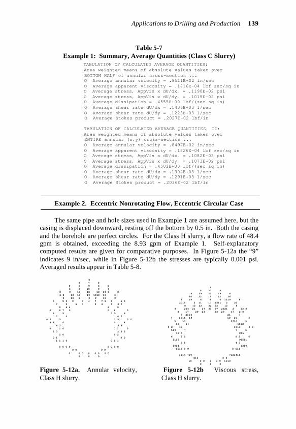
Applications to Drilling and Production 139
Table 5-7Example 1: Summary, Average Quantities (Class C Slurry)
TABULATION OF CALCULATED AVERAGE QUANTITIES: Area weighted means of absolute values taken over BOTTOM HALF of annular cross-section ... O Average annular velocity = .8511E+02 in/sec O Average apparent viscosity = .1816E-04 lbf sec/sq in O Average stress, AppVis x dU/dx, = .1190E-02 psi O Average stress, AppVis x dU/dy, = .1015E-02 psi O Average dissipation = .4555E+00 lbf/(sec sq in) O Average shear rate dU/dx = .1436E+03 1/sec O Average shear rate dU/dy = .1223E+03 1/sec O Average Stokes product = .2027E-02 lbf/in
TABULATION OF CALCULATED AVERAGE QUANTITIES, II: Area weighted means of absolute values taken over ENTIRE annular (x,y) cross-section ... O Average annular velocity = .8497E+02 in/sec O Average apparent viscosity = .1826E-04 lbf sec/sq in O Average stress, AppVis x dU/dx, = .1082E-02 psi O Average stress, AppVis x dU/dy, = .1073E-02 psi O Average dissipation = .4502E+00 lbf/(sec sq in) O Average shear rate dU/dx = .1304E+03 1/sec O Average shear rate dU/dy = .1291E+03 1/sec O Average Stokes product = .2036E-02 lbf/in
Example 2. Eccentric Nonrotating Flow, Eccentric Circular Case
The same pipe and hole sizes used in Example 1 are assumed here, but thecasing is displaced downward, resting off the bottom by 0.5 in. Both the casingand the borehole are perfect circles. For the Class H slurry, a flow rate of 48.4gpm is obtained, exceeding the 8.93 gpm of Example 1. Self-explanatorycomputed results are given for comparative purposes. In Figure 5-12a the “9”indicates 9 in/sec, while in Figure 5-12b the stresses are typically 0.001 psi.Averaged results appear in Table 5-8.
0 0 7 0 0 6 9 6 0 6 9 10 9 6 0 9 10 10 10 10 9 0 6 8 10 10 10 1010 10 6 9 10 9 9 9 10 9 0 9 9 9 7 4 7 7 9 9 5 0 7 9 4 0 0 4 9 8 7 8 6 4 6 8 0 8 7 0 0 8 0 6 5 3 5 6 7 0 6 7 0 2 5 2 5 2 0 4 4 0 0 4 4 2 3 4 0 1 0 0 1 0 2 3 2 3 2 2 0 0 2 0 1 0 0 1 1 1 0 0 1 1
0 0 0 0 0 0 0 0 0 0 0 0
0 0 0 0 0 0 0 0 0 0 0
Figure 5-12a. Annular velocity,Class H slurry.
3 4 30 4 6 29 22 29 6 26 22 15 22 26 8 19 6 8 6 1219 8 2015 2 11 17 1511 2 20 8 12 22 22 22 12 8 8 214 21 27 33 27 2521 2 13 8 8 17 29 23 23 29 17 2 8 7 2124 21 7 4 1515 19 19 15 4 1 17 1717 1 12 14 1512 0 2 13 1013 2 0 510 7 7 5 15 5 815
6 2 0 0 2 6 1115 91511 3 5 4 3 1014 1310 1515 0 9 8 515
1114 710 7121411 810 8 8 10 0 8 3 3 0 1010 8 6 8
Figure 5-12b Viscous stress,Class H slurry.

140 Computational Rheology
0 0 38 0 0 37 56 37 0 35 55 63 55 35 0 52 64 64 64 5952 0 3147 61 64 62 6164 61 31 54 61 55 56 55 61 54 0 5656 52 44 26 44 4152 56 26 0 40 53 24 0 0 24 53 4640 48 3621 36 48 0 4438 0 0 44 0 31 29 1529 31 37 0 3437 014 29 1229 14 0 2225 0 0 22 2514 1925 0 7 0 0 7 0 1315 131513 11 0 411 0 6 4 0 7 8 5 0 2 6 7
0 3 3 1 1 3 2 0 1 0 0 1 0 0 0 0 0 0 1 0 0 0 0
Figure 5-12c. Annular velocity, Class C slurry.
Table 5-8Example 2: Summary, Average Quantities (Class H Slurry)
TABULATION OF CALCULATED AVERAGE QUANTITIES: Area weighted means of absolute values taken over BOTTOM HALF of annular cross-section ... O Average annular velocity = .5958E+00 in/sec O Average apparent viscosity = .2206E-02 lbf sec/sq in O Average stress, AppVis x dU/dx, = .8796E-03 psi O Average stress, AppVis x dU/dy, = .1014E-02 psi O Average dissipation = .4405E-02 lbf/(sec sq in) O Average shear rate dU/dx = .1097E+01 1/sec O Average shear rate dU/dy = .1796E+01 1/sec O Average Stokes product = .5406E-03 lbf/in
TABULATION OF CALCULATED AVERAGE QUANTITIES, II: Area weighted means of absolute values taken over ENTIRE annular (x,y) cross-section ... O Average annular velocity = .3470E+01 in/sec O Average apparent viscosity = .1302E-02 lbf sec/sq in O Average stress, AppVis x dU/dx, = .1171E-02 psi O Average stress, AppVis x dU/dy, = .1201E-02 psi O Average dissipation = .1560E-01 lbf/(sec sq in) O Average shear rate dU/dx = .4129E+01 1/sec O Average shear rate dU/dy = .4283E+01 1/sec O Average Stokes product = .2691E-02 lbf/in
The calculations for this circular eccentric casing and hole are nowrepeated for the Class C slurry. Here, the volume flow rate is 2,706 gal/min.Computed results for the velocity distribution are shown in Figure 5-12c, where“60” indicates 600 in/sec; averaged results are recorded in Table 5-9.
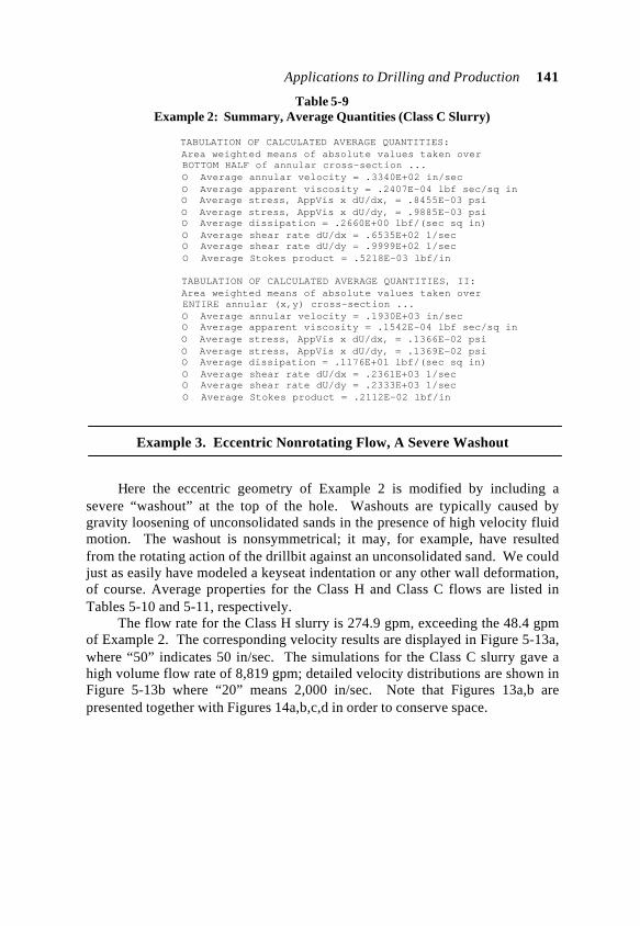
Applications to Drilling and Production 141
Table 5-9Example 2: Summary, Average Quantities (Class C Slurry)
TABULATION OF CALCULATED AVERAGE QUANTITIES: Area weighted means of absolute values taken over BOTTOM HALF of annular cross-section ... O Average annular velocity = .3340E+02 in/sec O Average apparent viscosity = .2407E-04 lbf sec/sq in O Average stress, AppVis x dU/dx, = .8455E-03 psi O Average stress, AppVis x dU/dy, = .9885E-03 psi O Average dissipation = .2660E+00 lbf/(sec sq in) O Average shear rate dU/dx = .6535E+02 1/sec O Average shear rate dU/dy = .9999E+02 1/sec O Average Stokes product = .5218E-03 lbf/in
TABULATION OF CALCULATED AVERAGE QUANTITIES, II: Area weighted means of absolute values taken over ENTIRE annular (x,y) cross-section ... O Average annular velocity = .1930E+03 in/sec O Average apparent viscosity = .1542E-04 lbf sec/sq in O Average stress, AppVis x dU/dx, = .1366E-02 psi O Average stress, AppVis x dU/dy, = .1369E-02 psi O Average dissipation = .1176E+01 lbf/(sec sq in) O Average shear rate dU/dx = .2361E+03 1/sec O Average shear rate dU/dy = .2333E+03 1/sec O Average Stokes product = .2112E-02 lbf/in
Example 3. Eccentric Nonrotating Flow, A Severe Washout
Here the eccentric geometry of Example 2 is modified by including asevere “washout” at the top of the hole. Washouts are typically caused bygravity loosening of unconsolidated sands in the presence of high velocity fluidmotion. The washout is nonsymmetrical; it may, for example, have resultedfrom the rotating action of the drillbit against an unconsolidated sand. We couldjust as easily have modeled a keyseat indentation or any other wall deformation,of course. Average properties for the Class H and Class C flows are listed inTables 5-10 and 5-11, respectively.
The flow rate for the Class H slurry is 274.9 gpm, exceeding the 48.4 gpmof Example 2. The corresponding velocity results are displayed in Figure 5-13a,where “50” indicates 50 in/sec. The simulations for the Class C slurry gave ahigh volume flow rate of 8,819 gpm; detailed velocity distributions are shown inFigure 5-13b where “20” means 2,000 in/sec. Note that Figures 13a,b arepresented together with Figures 14a,b,c,d in order to conserve space.
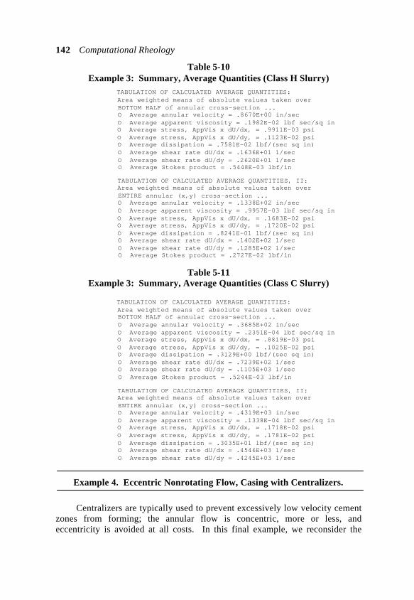
142 Computational Rheology
Table 5-10Example 3: Summary, Average Quantities (Class H Slurry) TABULATION OF CALCULATED AVERAGE QUANTITIES: Area weighted means of absolute values taken over BOTTOM HALF of annular cross-section ... O Average annular velocity = .8670E+00 in/sec O Average apparent viscosity = .1982E-02 lbf sec/sq in O Average stress, AppVis x dU/dx, = .9911E-03 psi O Average stress, AppVis x dU/dy, = .1123E-02 psi O Average dissipation = .7581E-02 lbf/(sec sq in) O Average shear rate dU/dx = .1636E+01 1/sec O Average shear rate dU/dy = .2620E+01 1/sec O Average Stokes product = .5448E-03 lbf/in
TABULATION OF CALCULATED AVERAGE QUANTITIES, II: Area weighted means of absolute values taken over ENTIRE annular (x,y) cross-section ... O Average annular velocity = .1338E+02 in/sec O Average apparent viscosity = .9957E-03 lbf sec/sq in O Average stress, AppVis x dU/dx, = .1683E-02 psi O Average stress, AppVis x dU/dy, = .1720E-02 psi O Average dissipation = .8241E-01 lbf/(sec sq in) O Average shear rate dU/dx = .1402E+02 1/sec O Average shear rate dU/dy = .1285E+02 1/sec O Average Stokes product = .2727E-02 lbf/in
Table 5-11Example 3: Summary, Average Quantities (Class C Slurry)
TABULATION OF CALCULATED AVERAGE QUANTITIES: Area weighted means of absolute values taken over BOTTOM HALF of annular cross-section ... O Average annular velocity = .3685E+02 in/sec O Average apparent viscosity = .2351E-04 lbf sec/sq in O Average stress, AppVis x dU/dx, = .8819E-03 psi O Average stress, AppVis x dU/dy, = .1025E-02 psi O Average dissipation = .3129E+00 lbf/(sec sq in) O Average shear rate dU/dx = .7239E+02 1/sec O Average shear rate dU/dy = .1105E+03 1/sec O Average Stokes product = .5244E-03 lbf/in
TABULATION OF CALCULATED AVERAGE QUANTITIES, II: Area weighted means of absolute values taken over ENTIRE annular (x,y) cross-section ... O Average annular velocity = .4319E+03 in/sec O Average apparent viscosity = .1338E-04 lbf sec/sq in O Average stress, AppVis x dU/dx, = .1718E-02 psi O Average stress, AppVis x dU/dy, = .1781E-02 psi O Average dissipation = .3035E+01 lbf/(sec sq in) O Average shear rate dU/dx = .4546E+03 1/sec O Average shear rate dU/dy = .4245E+03 1/sec
Example 4. Eccentric Nonrotating Flow, Casing with Centralizers.
Centralizers are typically used to prevent excessively low velocity cementzones from forming; the annular flow is concentric, more or less, andeccentricity is avoided at all costs. In this final example, we reconsider the
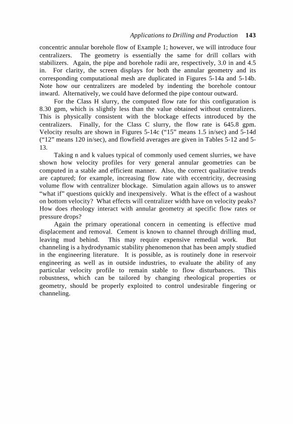
Applications to Drilling and Production 143
concentric annular borehole flow of Example 1; however, we will introduce fourcentralizers. The geometry is essentially the same for drill collars withstabilizers. Again, the pipe and borehole radii are, respectively, 3.0 in and 4.5in. For clarity, the screen displays for both the annular geometry and itscorresponding computational mesh are duplicated in Figures 5-14a and 5-14b.Note how our centralizers are modeled by indenting the borehole contourinward. Alternatively, we could have deformed the pipe contour outward.
For the Class H slurry, the computed flow rate for this configuration is8.30 gpm, which is slightly less than the value obtained without centralizers.This is physically consistent with the blockage effects introduced by thecentralizers. Finally, for the Class C slurry, the flow rate is 645.8 gpm.Velocity results are shown in Figures 5-14c (“15” means 1.5 in/sec) and 5-14d(“12” means 120 in/sec), and flowfield averages are given in Tables 5-12 and 5-13.
Taking n and k values typical of commonly used cement slurries, we haveshown how velocity profiles for very general annular geometries can becomputed in a stable and efficient manner. Also, the correct qualitative trendsare captured; for example, increasing flow rate with eccentricity, decreasingvolume flow with centralizer blockage. Simulation again allows us to answer“what if” questions quickly and inexpensively. What is the effect of a washouton bottom velocity? What effects will centralizer width have on velocity peaks?How does rheology interact with annular geometry at specific flow rates orpressure drops?
Again the primary operational concern in cementing is effective muddisplacement and removal. Cement is known to channel through drilling mud,leaving mud behind. This may require expensive remedial work. Butchanneling is a hydrodynamic stability phenomenon that has been amply studiedin the engineering literature. It is possible, as is routinely done in reservoirengineering as well as in outside industries, to evaluate the ability of anyparticular velocity profile to remain stable to flow disturbances. Thisrobustness, which can be tailored by changing rheological properties orgeometry, should be properly exploited to control undesirable fingering orchanneling.
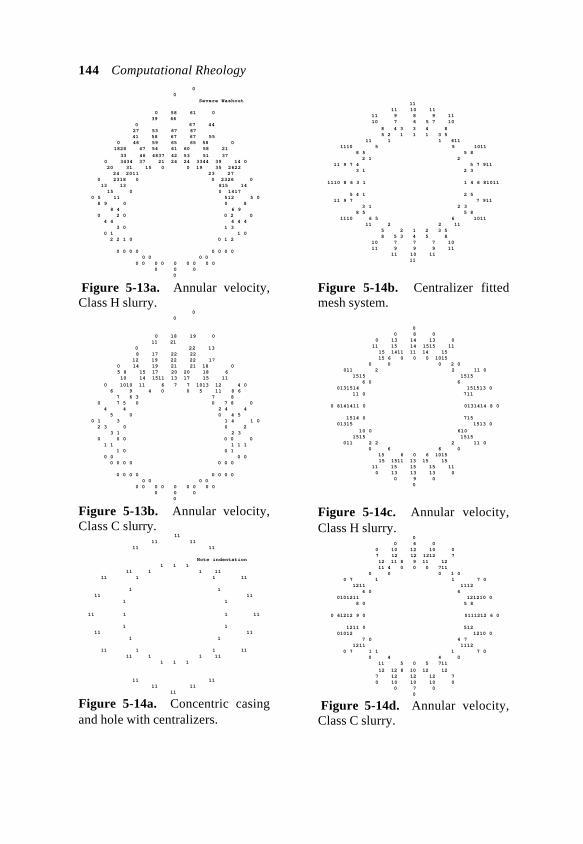
144 Computational Rheology 0 0 Severe Washout
0 58 61 0 39 66 0 67 44 27 53 67 67 41 58 67 67 55 0 46 59 65 65 58 0 1828 47 54 61 60 58 21
33 46 4837 42 53 51 37 0 3434 37 21 24 24 3344 39 14 0 20 31 15 0 0 19 35 2622 24 2011 23 27 0 2318 0 0 2326 0 13 13 815 14 15 0 0 1417 0 5 11 512 5 0 8 9 0 0 8 8 4 6 9 0 2 0 0 2 0 4 4 4 4 4 3 0 1 3 0 1 1 0 2 2 1 0 0 1 2
0 0 0 0 0 0 0 0 0 0 0 0 0 0 0 0 0 0 0 0 0 0 0 0 0
Figure 5-13a. Annular velocity,Class H slurry. 0 0
0 18 19 0 11 21 0 22 13 8 17 22 22 12 19 22 22 17 0 14 19 21 21 18 0 5 8 15 17 20 20 18 6 10 14 1511 13 17 15 11
0 1010 11 6 7 7 1013 12 4 0 6 9 4 0 0 5 11 8 6 7 6 3 7 8 0 7 5 0 0 7 8 0 4 4 2 4 4 5 0 0 4 5 0 1 3 1 4 1 0 2 3 0 0 2 3 1 2 3 0 0 0 0 0 0 1 1 1 1 1 1 0 0 1 0 0 0 0 0 0 0 0 0 0 0
0 0 0 0 0 0 0 0 0 0 0 0 0 0 0 0 0 0 0 0 0 0 0 0 0
Figure 5-13b. Annular velocity,Class C slurry. 11 11 11 11 11
Note indentation 1 1 1 11 1 1 11 11 1 1 11
1 1 11 11 1 1
11 1 1 11
1 1 11 11 1 1
11 1 1 11 11 1 1 11 1 1 1
11 11 11 11 11
Figure 5-14a. Concentric casingand hole with centralizers.
11 11 10 11 11 9 8 9 11 10 7 6 5 7 10
8 4 3 3 4 8 5 2 1 1 1 3 5 11 1 1 611 1110 5 5 1011 8 5 5 8 2 1 2 11 9 7 4 5 7 911 3 1 2 3
1110 8 6 3 1 1 4 6 81011
5 4 1 2 5 11 9 7 7 911 3 1 2 3 8 5 5 8 1110 6 5 6 1011 11 2 2 11 5 2 1 2 3 5 8 5 3 4 5 8 10 7 7 7 10 11 9 9 9 11 11 10 11 11
Figure 5-14b. Centralizer fittedmesh system.
0 0 8 0 0 13 14 13 0 11 15 14 1515 11 15 1411 11 14 15 15 6 0 0 0 1015 0 0 0 2 0 011 2 2 11 0 1515 1515 6 0 6 0131514 151513 0 11 0 711
0 8141411 0 0131414 8 0
1514 0 715 01315 1513 0
10 0 610 1515 1515 011 2 2 2 11 0 0 6 6 0 15 6 0 6 1015 15 1511 13 15 15 11 15 15 15 11 0 13 13 13 0 0 9 0 0
Figure 5-14c. Annular velocity,Class H slurry. 0 0 6 0 0 10 12 10 0 7 12 12 1212 7 12 11 8 9 11 12 11 4 0 0 0 711 0 0 0 1 0 0 7 1 1 7 0 1211 1112 4 0 4 0101211 121210 0 8 0 5 8
0 61212 9 0 0111212 6 0
1211 0 512 01012 1210 0 7 0 4 7 1211 1112 0 7 1 1 1 7 0 0 4 4 0 11 5 0 5 711
12 12 8 10 12 12 7 12 12 12 7 0 10 10 10 0 0 7 0 0
Figure 5-14d. Annular velocity,Class C slurry.
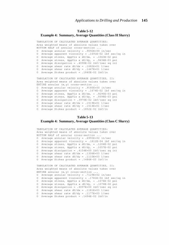
Applications to Drilling and Production 145
Table 5-12Example 4: Summary, Average Quantities (Class H Slurry)
TABULATION OF CALCULATED AVERAGE QUANTITIES: Area weighted means of absolute values taken over BOTTOM HALF of annular cross-section ... O Average annular velocity = .9092E+00 in/sec O Average apparent viscosity = .1691E-02 lbf sec/sq in O Average stress, AppVis x dU/dx, = .1063E-02 psi O Average stress, AppVis x dU/dy, = .9636E-03 psi O Average dissipation = .4090E-02 lbf/(sec sq in) O Average shear rate dU/dx = .1682E+01 1/sec O Average shear rate dU/dy = .1447E+01 1/sec O Average Stokes product = .1840E-02 lbf/in
TABULATION OF CALCULATED AVERAGE QUANTITIES, II: Area weighted means of absolute values taken over ENTIRE annular (x,y) cross-section ... O Average annular velocity = .9185E+00 in/sec O Average apparent viscosity = .1674E-02 lbf sec/sq in O Average stress, AppVis x dU/dx, = .9290E-03 psi O Average stress, AppVis x dU/dy, = .9398E-03 psi O Average dissipation = .3970E-02 lbf/(sec sq in) O Average shear rate dU/dx = .1519E+01 1/sec O Average shear rate dU/dy = .1514E+01 1/sec O Average Stokes product = .1852E-02 lbf/in
Table 5-13Example 4: Summary, Average Quantities (Class C Slurry)
TABULATION OF CALCULATED AVERAGE QUANTITIES: Area weighted means of absolute values taken over BOTTOM HALF of annular cross-section ... O Average annular velocity = .6993E+02 in/sec O Average apparent viscosity = .1812E-04 lbf sec/sq in O Average stress, AppVis x dU/dx, = .1206E-02 psi O Average stress, AppVis x dU/dy, = .1057E-02 psi O Average dissipation = .4154E+00 lbf/(sec sq in) O Average shear rate dU/dx = .1306E+03 1/sec O Average shear rate dU/dy = .1110E+03 1/sec O Average Stokes product = .1486E-02 lbf/in
TABULATION OF CALCULATED AVERAGE QUANTITIES, II: Area weighted means of absolute values taken over ENTIRE annular (x,y) cross-section ... O Average annular velocity = .7129E+02 in/sec O Average apparent viscosity = .1781E-04 lbf sec/sq in O Average stress, AppVis x dU/dx, = .1076E-02 psi O Average stress, AppVis x dU/dy, = .1078E-02 psi O Average dissipation = .4097E+00 lbf/(sec sq in) O Average shear rate dU/dx = .1181E+03 1/sec O Average shear rate dU/dy = .1177E+03 1/sec O Average Stokes product = .1494E-02 lbf/in

146 Computational Rheology
Example 5. Concentric Rotating Flows, Stationary Baseline
While cement slurry displaces drilling fluid in the annulus, the casing isoften rotated from 10-20 rpm. The reasons are twofold: first to break the gelstrength of any coagulated mud, and second to prevent flowing mud fromgelling. The latter is amenable to flow simulation and modeling. It is of interestto compare the stress states for stationary versus rotating casings. We willassume a concentric geometry and use the analytical results of Chapter 3obtained for rotating pipes. Again, the closed form expressions require a narrowannulus. The input summary shown in Table 5-14, extracted from output files,establishes reference conditions for a nonrotating flow run with “0.001 rpm.”For stationary casings, the exact solution is of course available; however, forcomparative reasons, we will not make use of it.
Table 5-14Summary of Input Parameters
O Drillpipe outer radius (inches) = 4.0000 O Borehole radius (inches) = 5.0000 O Axial pressure gradient (psi/ft) = .01000 O Drillstring rotation rate (rpm) = .0010 O Drillstring rotation rate (rad/sec) = .0001 O Fluid exponent "n" (nondimensional) = .7240
O Consistency factor (lbf secn/sq in) = .1861E-04
O Mass density of fluid (lbf sec2/ft4) = 1.9000 (e.g., about 1.9 for water) O Number of radial "grid" positions = 17
The software model calculates all physical quantities of possible interest.These include the variables discussed in Chapter 3, and, in addition, severalderivative flow properties. The complete roster of output variables is given inTable 5-15; this same chart is supplied with all computed results.
Calculations for the foregoing quantities at each of the 17 control pointsselected in Table 5-14 require less than one second on Pentium machines.Various types of output are provided for correlation or research purposes, e.g.,“high level” results such as,
Total volume flow rate (cubic in/sec) = .2653E+03 (gal/min) = .6889E+02
Or “low level results” conveniently supplied in hybrid text and ASCII plot formfor complete portability; for example, Figure 5-15a for annular velocity orFigure 5-15b for the “maximum stress” defined in Table 5-15 next.
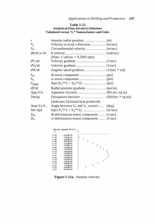
Applications to Drilling and Production 147
Table 5-15Analytical (Non-Iterative) Solutions
Tabulated versus “r,” Nomenclature and Units
r Annular radial position ...........………. (in)Vz Velocity in axial z direction .………… (in/sec)Vθ Circumferential velocity ......…………. (in/sec)dθ/dt or W θ velocity ...................……………….. (rad/sec) (Note: 1 rad/sec = 9.5493 rpm)dVz/dr Velocity gradient ..............…………… (1/sec)dVθ/dr Velocity gradient ..............…………… (1/sec)dW/dr Angular speed gradient ..…………….. (1/(sec × in))
Srθ rθ stress component ..............………… (psi)Srz rz stress component ..............………… (psi)Smax Sqrt (Srz**2 + Srθ**2) ...........………... (psi)
dP/dr Radial pressure gradient ......…………. (psi/in)App-Vis Apparent viscosity ....………………… (lbf sec /sq in)Dissip Dissipation function …………………. (lbf/(sec × sq in)) (indicates frictional heat produced)Atan Vθ/Vz Angle between Vθ and Vz vectors ..… (deg)Net Spd Sqrt (Vz**2 + Vθ**2) ..........………… (in/sec)Drθ rθ deformation tensor component …… (1/sec)Drz rz deformation tensor component …… (1/sec)
Axial speed Vz(r): r 0 ______________________________ 5.00 -.2578E-05 | 4.94 .1383E+01 |* 4.88 .3393E+01 | * 4.82 .5570E+01 | * 4.76 .7731E+01 | * 4.71 .9759E+01 | * 4.65 .1156E+02 | * 4.59 .1307E+02 | * 4.53 .1421E+02 | * 4.47 .1494E+02 | * 4.41 .1519E+02 | * 4.35 .1493E+02 | * 4.29 .1410E+02 | * 4.24 .1267E+02 | * 4.18 .1058E+02 | * 4.12 .7797E+01 | * 4.06 .4285E+01 | * 4.00 .0000E+00 |
Figure 5-15a. Annular velocity.

148 Computational Rheology
Maximum stress Smax (r): r 0 ______________________________ 5.00 .3958E-03 | * 4.94 .3512E-03 | * 4.88 .3062E-03 | * 4.82 .2606E-03 | * 4.76 .2145E-03 | * 4.71 .1678E-03 | * 4.65 .1206E-03 | * 4.59 .7282E-04 | * 4.53 .2443E-04 * 4.47 .2459E-04 * 4.41 .7426E-04 | * 4.35 .1246E-03 | * 4.29 .1757E-03 | * 4.24 .2275E-03 | * 4.18 .2801E-03 | * 4.12 .3334E-03 | * 4.06 .3876E-03 | * 4.00 .4427E-03 | *
Figure 5-15b. Maximum stress.
Detailed listings are also available for permanent reference; flowproperties, tabulated against “r,” can be read by spreadsheet programs for furthertrend analysis. A complete summary of computed results appears in Tables 5-16to 5-19.
Table 5-16Averaged Values of Annular Quantities
Average Vz (in/sec) = .9480E+01 (ft/min) = .4740E+02 Average Vθ (in/sec) = .3253E-02 Average W (rad/sec) = .7401E-03 Average total speed (in/sec) = .9480E+01 Average angle between Vz and VÕ (deg) = .2633E+01 Average d(Vz)/dr (1/sec) = .0000E+00 Average d(Vθ)/dr (1/sec) = -.8717E-02
Average dW/dr (1/(sec × in)) = -.2136E-02 Average dP/dr (psi/in) = .2709E-09 Average Srθ (psi) = .7355E-07 Average Srz (psi) = .7828E-05 Average Smax (psi) = .2097E-03 Average dissipation function (lbf sec^n-2/sq in) =.9225E-02 Average apparent viscosity (lbf sec^n/sq in) = .8692E-05 Average Drθ (1/sec) = .4729E-02 Average Drz (1/sec) = .8465E+00
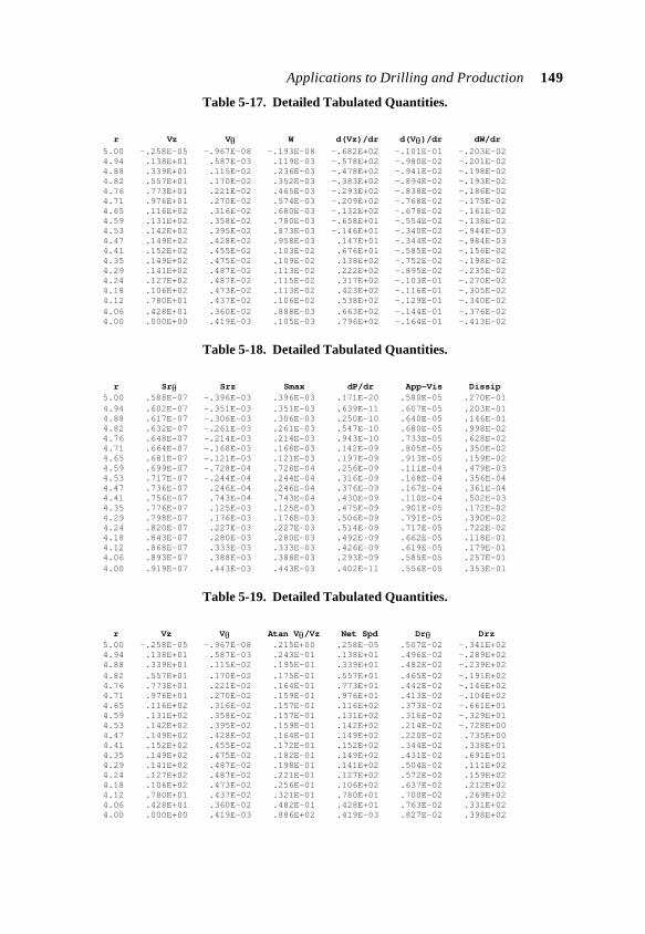
Applications to Drilling and Production 149
Table 5-17. Detailed Tabulated Quantities.
r Vz Vθ W d(Vz)/dr d(Vθ)/dr dW/dr 5.00 -.258E-05 -.967E-08 -.193E-08 -.682E+02 -.101E-01 -.203E-02 4.94 .138E+01 .587E-03 .119E-03 -.578E+02 -.980E-02 -.201E-02 4.88 .339E+01 .115E-02 .236E-03 -.478E+02 -.941E-02 -.198E-02 4.82 .557E+01 .170E-02 .352E-03 -.383E+02 -.894E-02 -.193E-02 4.76 .773E+01 .221E-02 .465E-03 -.293E+02 -.838E-02 -.186E-02 4.71 .976E+01 .270E-02 .574E-03 -.209E+02 -.768E-02 -.175E-02 4.65 .116E+02 .316E-02 .680E-03 -.132E+02 -.678E-02 -.161E-02 4.59 .131E+02 .358E-02 .780E-03 -.658E+01 -.554E-02 -.138E-02 4.53 .142E+02 .395E-02 .873E-03 -.146E+01 -.340E-02 -.944E-03 4.47 .149E+02 .428E-02 .958E-03 .147E+01 -.344E-02 -.984E-03 4.41 .152E+02 .455E-02 .103E-02 .676E+01 -.585E-02 -.156E-02 4.35 .149E+02 .475E-02 .109E-02 .138E+02 -.752E-02 -.198E-02 4.29 .141E+02 .487E-02 .113E-02 .222E+02 -.895E-02 -.235E-02 4.24 .127E+02 .487E-02 .115E-02 .317E+02 -.103E-01 -.270E-02 4.18 .106E+02 .473E-02 .113E-02 .423E+02 -.116E-01 -.305E-02 4.12 .780E+01 .437E-02 .106E-02 .538E+02 -.129E-01 -.340E-02 4.06 .428E+01 .360E-02 .888E-03 .663E+02 -.144E-01 -.376E-02 4.00 .000E+00 .419E-03 .105E-03 .796E+02 -.164E-01 -.413E-02
Table 5-18. Detailed Tabulated Quantities.
r Srθ Srz Smax dP/dr App-Vis Dissip 5.00 .588E-07 -.396E-03 .396E-03 .171E-20 .580E-05 .270E-01 4.94 .602E-07 -.351E-03 .351E-03 .639E-11 .607E-05 .203E-01 4.88 .617E-07 -.306E-03 .306E-03 .250E-10 .640E-05 .146E-01 4.82 .632E-07 -.261E-03 .261E-03 .547E-10 .680E-05 .998E-02 4.76 .648E-07 -.214E-03 .214E-03 .943E-10 .733E-05 .628E-02 4.71 .664E-07 -.168E-03 .168E-03 .142E-09 .805E-05 .350E-02 4.65 .681E-07 -.121E-03 .121E-03 .197E-09 .913E-05 .159E-02 4.59 .699E-07 -.728E-04 .728E-04 .256E-09 .111E-04 .479E-03 4.53 .717E-07 -.244E-04 .244E-04 .316E-09 .168E-04 .356E-04 4.47 .736E-07 .246E-04 .246E-04 .376E-09 .167E-04 .361E-04 4.41 .756E-07 .743E-04 .743E-04 .430E-09 .110E-04 .502E-03 4.35 .776E-07 .125E-03 .125E-03 .475E-09 .901E-05 .172E-02 4.29 .798E-07 .176E-03 .176E-03 .506E-09 .791E-05 .390E-02 4.24 .820E-07 .227E-03 .227E-03 .514E-09 .717E-05 .722E-02 4.18 .843E-07 .280E-03 .280E-03 .492E-09 .662E-05 .118E-01 4.12 .868E-07 .333E-03 .333E-03 .426E-09 .619E-05 .179E-01 4.06 .893E-07 .388E-03 .388E-03 .293E-09 .585E-05 .257E-01 4.00 .919E-07 .443E-03 .443E-03 .402E-11 .556E-05 .353E-01
Table 5-19. Detailed Tabulated Quantities.
r Vz Vθ Atan Vθ/Vz Net Spd Drθ Drz 5.00 -.258E-05 -.967E-08 .215E+00 .258E-05 .507E-02 -.341E+02 4.94 .138E+01 .587E-03 .243E-01 .138E+01 .496E-02 -.289E+02 4.88 .339E+01 .115E-02 .195E-01 .339E+01 .482E-02 -.239E+02 4.82 .557E+01 .170E-02 .175E-01 .557E+01 .465E-02 -.191E+02 4.76 .773E+01 .221E-02 .164E-01 .773E+01 .442E-02 -.146E+02 4.71 .976E+01 .270E-02 .159E-01 .976E+01 .413E-02 -.104E+02 4.65 .116E+02 .316E-02 .157E-01 .116E+02 .373E-02 -.661E+01 4.59 .131E+02 .358E-02 .157E-01 .131E+02 .316E-02 -.329E+01 4.53 .142E+02 .395E-02 .159E-01 .142E+02 .214E-02 -.728E+00 4.47 .149E+02 .428E-02 .164E-01 .149E+02 .220E-02 .735E+00 4.41 .152E+02 .455E-02 .172E-01 .152E+02 .344E-02 .338E+01 4.35 .149E+02 .475E-02 .182E-01 .149E+02 .431E-02 .691E+01 4.29 .141E+02 .487E-02 .198E-01 .141E+02 .504E-02 .111E+02 4.24 .127E+02 .487E-02 .221E-01 .127E+02 .572E-02 .159E+02 4.18 .106E+02 .473E-02 .256E-01 .106E+02 .637E-02 .212E+02 4.12 .780E+01 .437E-02 .321E-01 .780E+01 .700E-02 .269E+02 4.06 .428E+01 .360E-02 .482E-01 .428E+01 .763E-02 .331E+02 4.00 .000E+00 .419E-03 .886E+02 .419E-03 .827E-02 .398E+02
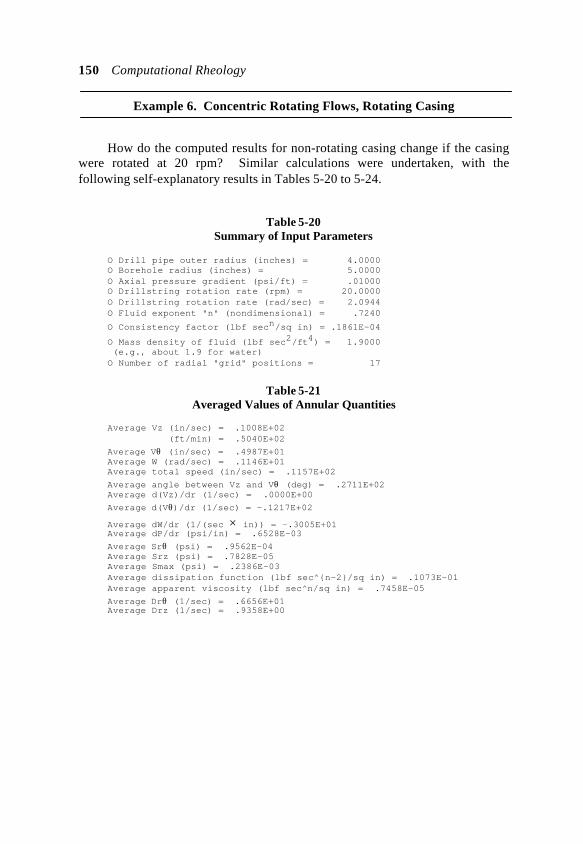
150 Computational Rheology
Example 6. Concentric Rotating Flows, Rotating Casing
How do the computed results for non-rotating casing change if the casingwere rotated at 20 rpm? Similar calculations were undertaken, with thefollowing self-explanatory results in Tables 5-20 to 5-24.
Table 5-20Summary of Input Parameters
O Drill pipe outer radius (inches) = 4.0000O Borehole radius (inches) = 5.0000O Axial pressure gradient (psi/ft) = .01000O Drillstring rotation rate (rpm) = 20.0000O Drillstring rotation rate (rad/sec) = 2.0944O Fluid exponent "n" (nondimensional) = .7240
O Consistency factor (lbf secn/sq in) = .1861E-04
O Mass density of fluid (lbf sec2/ft4) = 1.9000 (e.g., about 1.9 for water)O Number of radial "grid" positions = 17
Table 5-21Averaged Values of Annular Quantities
Average Vz (in/sec) = .1008E+02 (ft/min) = .5040E+02
Average Vθ (in/sec) = .4987E+01Average W (rad/sec) = .1146E+01Average total speed (in/sec) = .1157E+02
Average angle between Vz and Vθ (deg) = .2711E+02Average d(Vz)/dr (1/sec) = .0000E+00
Average d(Vθ)/dr (1/sec) = -.1217E+02
Average dW/dr (1/(sec × in)) = -.3005E+01Average dP/dr (psi/in) = .6528E-03
Average Srθ (psi) = .9562E-04Average Srz (psi) = .7828E-05Average Smax (psi) = .2386E-03Average dissipation function (lbf sec^n-2/sq in) = .1073E-01Average apparent viscosity (lbf sec^n/sq in) = .7458E-05
Average Drθ (1/sec) = .6656E+01Average Drz (1/sec) = .9358E+00
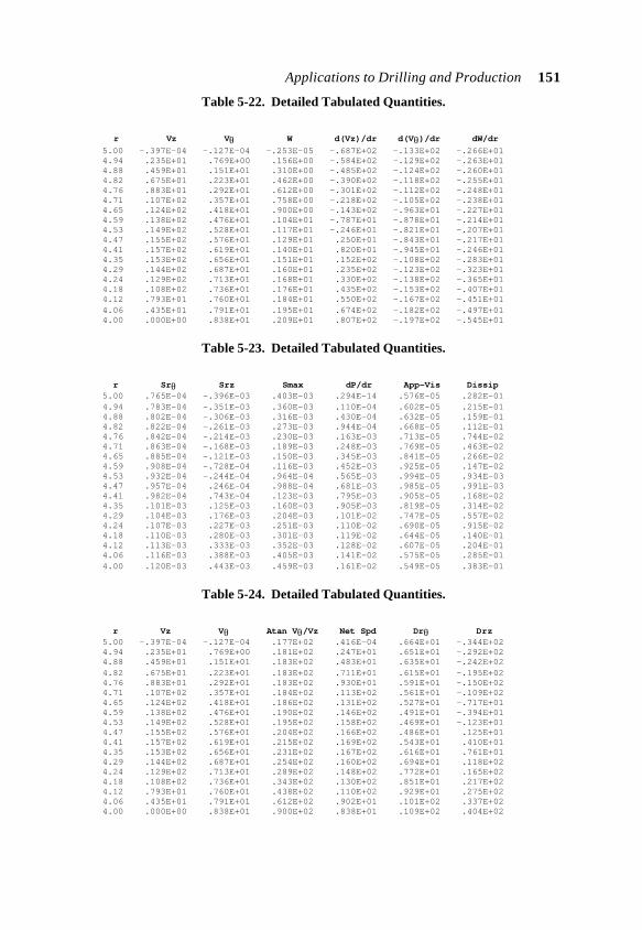
Applications to Drilling and Production 151
Table 5-22. Detailed Tabulated Quantities.
r Vz Vθ W d(Vz)/dr d(Vθ)/dr dW/dr 5.00 -.397E-04 -.127E-04 -.253E-05 -.687E+02 -.133E+02 -.266E+01 4.94 .235E+01 .769E+00 .156E+00 -.584E+02 -.129E+02 -.263E+01 4.88 .459E+01 .151E+01 .310E+00 -.485E+02 -.124E+02 -.260E+01 4.82 .675E+01 .223E+01 .462E+00 -.390E+02 -.118E+02 -.255E+01 4.76 .883E+01 .292E+01 .612E+00 -.301E+02 -.112E+02 -.248E+01 4.71 .107E+02 .357E+01 .758E+00 -.218E+02 -.105E+02 -.238E+01 4.65 .124E+02 .418E+01 .900E+00 -.143E+02 -.963E+01 -.227E+01 4.59 .138E+02 .476E+01 .104E+01 -.787E+01 -.878E+01 -.214E+01 4.53 .149E+02 .528E+01 .117E+01 -.246E+01 -.821E+01 -.207E+01 4.47 .155E+02 .576E+01 .129E+01 .250E+01 -.843E+01 -.217E+01 4.41 .157E+02 .619E+01 .140E+01 .820E+01 -.945E+01 -.246E+01 4.35 .153E+02 .656E+01 .151E+01 .152E+02 -.108E+02 -.283E+01 4.29 .144E+02 .687E+01 .160E+01 .235E+02 -.123E+02 -.323E+01 4.24 .129E+02 .713E+01 .168E+01 .330E+02 -.138E+02 -.365E+01 4.18 .108E+02 .736E+01 .176E+01 .435E+02 -.153E+02 -.407E+01 4.12 .793E+01 .760E+01 .184E+01 .550E+02 -.167E+02 -.451E+01 4.06 .435E+01 .791E+01 .195E+01 .674E+02 -.182E+02 -.497E+01 4.00 .000E+00 .838E+01 .209E+01 .807E+02 -.197E+02 -.545E+01
Table 5-23. Detailed Tabulated Quantities.
r Srθ Srz Smax dP/dr App-Vis Dissip 5.00 .765E-04 -.396E-03 .403E-03 .294E-14 .576E-05 .282E-01 4.94 .783E-04 -.351E-03 .360E-03 .110E-04 .602E-05 .215E-01 4.88 .802E-04 -.306E-03 .316E-03 .430E-04 .632E-05 .159E-01 4.82 .822E-04 -.261E-03 .273E-03 .944E-04 .668E-05 .112E-01 4.76 .842E-04 -.214E-03 .230E-03 .163E-03 .713E-05 .744E-02 4.71 .863E-04 -.168E-03 .189E-03 .248E-03 .769E-05 .463E-02 4.65 .885E-04 -.121E-03 .150E-03 .345E-03 .841E-05 .266E-02 4.59 .908E-04 -.728E-04 .116E-03 .452E-03 .925E-05 .147E-02 4.53 .932E-04 -.244E-04 .964E-04 .565E-03 .994E-05 .934E-03 4.47 .957E-04 .246E-04 .988E-04 .681E-03 .985E-05 .991E-03 4.41 .982E-04 .743E-04 .123E-03 .795E-03 .905E-05 .168E-02 4.35 .101E-03 .125E-03 .160E-03 .905E-03 .819E-05 .314E-02 4.29 .104E-03 .176E-03 .204E-03 .101E-02 .747E-05 .557E-02 4.24 .107E-03 .227E-03 .251E-03 .110E-02 .690E-05 .915E-02 4.18 .110E-03 .280E-03 .301E-03 .119E-02 .644E-05 .140E-01 4.12 .113E-03 .333E-03 .352E-03 .128E-02 .607E-05 .204E-01 4.06 .116E-03 .388E-03 .405E-03 .141E-02 .575E-05 .285E-01 4.00 .120E-03 .443E-03 .459E-03 .161E-02 .549E-05 .383E-01
Table 5-24. Detailed Tabulated Quantities.
r Vz Vθ Atan Vθ/Vz Net Spd Drθ Drz 5.00 -.397E-04 -.127E-04 .177E+02 .416E-04 .664E+01 -.344E+02 4.94 .235E+01 .769E+00 .181E+02 .247E+01 .651E+01 -.292E+02 4.88 .459E+01 .151E+01 .183E+02 .483E+01 .635E+01 -.242E+02 4.82 .675E+01 .223E+01 .183E+02 .711E+01 .615E+01 -.195E+02 4.76 .883E+01 .292E+01 .183E+02 .930E+01 .591E+01 -.150E+02 4.71 .107E+02 .357E+01 .184E+02 .113E+02 .561E+01 -.109E+02 4.65 .124E+02 .418E+01 .186E+02 .131E+02 .527E+01 -.717E+01 4.59 .138E+02 .476E+01 .190E+02 .146E+02 .491E+01 -.394E+01 4.53 .149E+02 .528E+01 .195E+02 .158E+02 .469E+01 -.123E+01 4.47 .155E+02 .576E+01 .204E+02 .166E+02 .486E+01 .125E+01 4.41 .157E+02 .619E+01 .215E+02 .169E+02 .543E+01 .410E+01 4.35 .153E+02 .656E+01 .231E+02 .167E+02 .616E+01 .761E+01 4.29 .144E+02 .687E+01 .254E+02 .160E+02 .694E+01 .118E+02 4.24 .129E+02 .713E+01 .289E+02 .148E+02 .772E+01 .165E+02 4.18 .108E+02 .736E+01 .343E+02 .130E+02 .851E+01 .217E+02 4.12 .793E+01 .760E+01 .438E+02 .110E+02 .929E+01 .275E+02 4.06 .435E+01 .791E+01 .612E+02 .902E+01 .101E+02 .337E+02 4.00 .000E+00 .838E+01 .900E+02 .838E+01 .109E+02 .404E+02
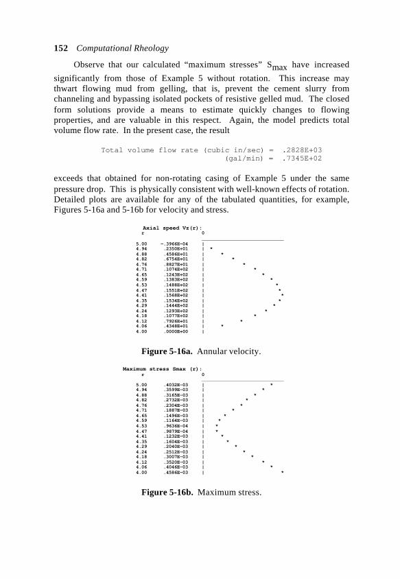
152 Computational Rheology
Observe that our calculated “maximum stresses” Smax have increased
significantly from those of Example 5 without rotation. This increase maythwart flowing mud from gelling, that is, prevent the cement slurry fromchanneling and bypassing isolated pockets of resistive gelled mud. The closedform solutions provide a means to estimate quickly changes to flowingproperties, and are valuable in this respect. Again, the model predicts totalvolume flow rate. In the present case, the result
Total volume flow rate (cubic in/sec) = .2828E+03 (gal/min) = .7345E+02
exceeds that obtained for non-rotating casing of Example 5 under the samepressure drop. This is physically consistent with well-known effects of rotation.Detailed plots are available for any of the tabulated quantities, for example,Figures 5-16a and 5-16b for velocity and stress.
Axial speed Vz(r): r 0 ______________________________ 5.00 -.3966E-04 | 4.94 .2350E+01 | * 4.88 .4586E+01 | * 4.82 .6754E+01 | * 4.76 .8827E+01 | * 4.71 .1074E+02 | * 4.65 .1243E+02 | * 4.59 .1383E+02 | * 4.53 .1488E+02 | * 4.47 .1551E+02 | * 4.41 .1568E+02 | * 4.35 .1534E+02 | * 4.29 .1444E+02 | * 4.24 .1293E+02 | * 4.18 .1077E+02 | * 4.12 .7926E+01 | * 4.06 .4348E+01 | * 4.00 .0000E+00 |
Figure 5-16a. Annular velocity.
Maximum stress Smax (r): r 0 ______________________________ 5.00 .4032E-03 | * 4.94 .3599E-03 | * 4.88 .3165E-03 | * 4.82 .2732E-03 | * 4.76 .2304E-03 | * 4.71 .1887E-03 | * 4.65 .1496E-03 | * 4.59 .1164E-03 | * 4.53 .9636E-04 | * 4.47 .9879E-04 | * 4.41 .1232E-03 | * 4.35 .1604E-03 | * 4.29 .2040E-03 | * 4.24 .2512E-03 | * 4.18 .3007E-03 | * 4.12 .3520E-03 | * 4.06 .4046E-03 | * 4.00 .4586E-03 | *
Figure 5-16b. Maximum stress.
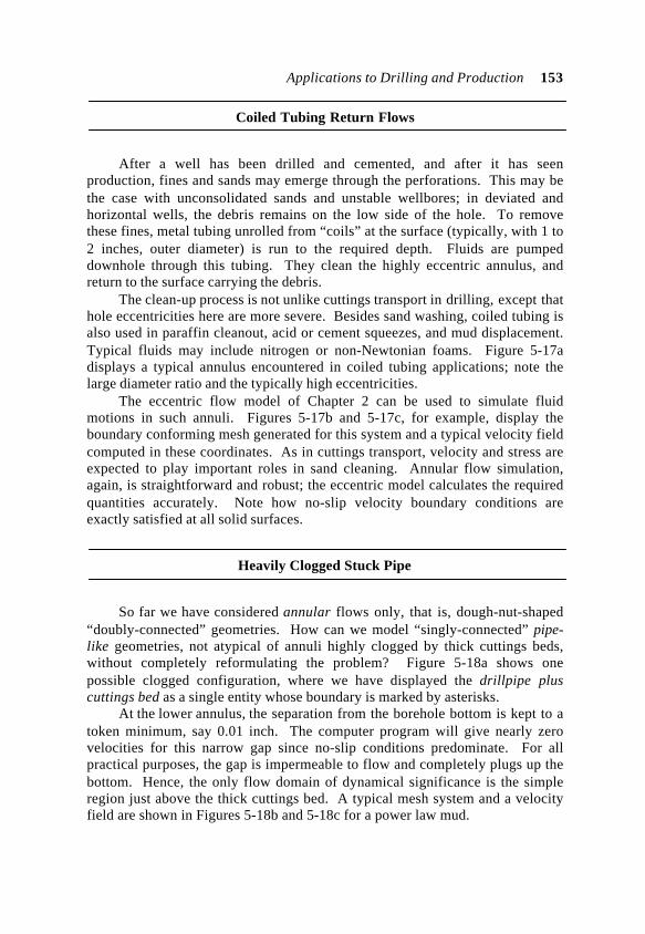
Applications to Drilling and Production 153
Coiled Tubing Return Flows
After a well has been drilled and cemented, and after it has seenproduction, fines and sands may emerge through the perforations. This may bethe case with unconsolidated sands and unstable wellbores; in deviated andhorizontal wells, the debris remains on the low side of the hole. To removethese fines, metal tubing unrolled from “coils” at the surface (typically, with 1 to2 inches, outer diameter) is run to the required depth. Fluids are pumpeddownhole through this tubing. They clean the highly eccentric annulus, andreturn to the surface carrying the debris.
The clean-up process is not unlike cuttings transport in drilling, except thathole eccentricities here are more severe. Besides sand washing, coiled tubing isalso used in paraffin cleanout, acid or cement squeezes, and mud displacement.Typical fluids may include nitrogen or non-Newtonian foams. Figure 5-17adisplays a typical annulus encountered in coiled tubing applications; note thelarge diameter ratio and the typically high eccentricities.
The eccentric flow model of Chapter 2 can be used to simulate fluidmotions in such annuli. Figures 5-17b and 5-17c, for example, display theboundary conforming mesh generated for this system and a typical velocity fieldcomputed in these coordinates. As in cuttings transport, velocity and stress areexpected to play important roles in sand cleaning. Annular flow simulation,again, is straightforward and robust; the eccentric model calculates the requiredquantities accurately. Note how no-slip velocity boundary conditions areexactly satisfied at all solid surfaces.
Heavily Clogged Stuck Pipe
So far we have considered annular flows only, that is, dough-nut-shaped“doubly-connected” geometries. How can we model “singly-connected” pipe-like geometries, not atypical of annuli highly clogged by thick cuttings beds,without completely reformulating the problem? Figure 5-18a shows onepossible clogged configuration, where we have displayed the drillpipe pluscuttings bed as a single entity whose boundary is marked by asterisks.
At the lower annulus, the separation from the borehole bottom is kept to atoken minimum, say 0.01 inch. The computer program will give nearly zerovelocities for this narrow gap since no-slip conditions predominate. For allpractical purposes, the gap is impermeable to flow and completely plugs up thebottom. Hence, the only flow domain of dynamical significance is the simpleregion just above the thick cuttings bed. A typical mesh system and a velocityfield are shown in Figures 5-18b and 5-18c for a power law mud.
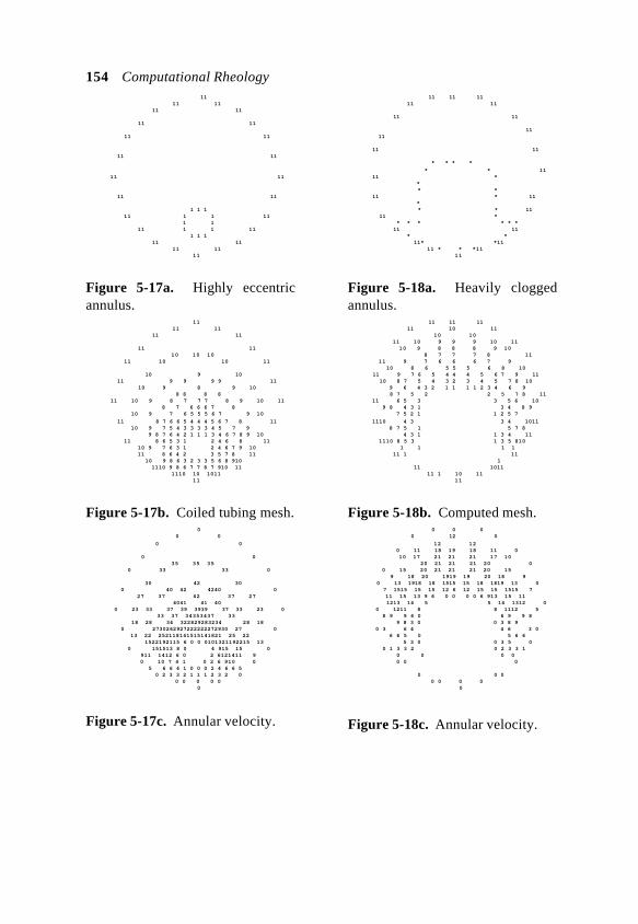
154 Computational Rheology 11 11 11 11 11
11 11
11 11
11 11
11 11
11 11
1 1 1 11 1 1 11 1 1 11 1 1 11 1 1 1 11 11 11 11 11
Figure 5-17a. Highly eccentricannulus. 11 11 11 11 11
11 11 10 10 10 11 10 10 11
10 9 10 11 9 9 9 9 11 10 9 8 9 10 8 8 8 8 11 10 9 8 7 7 7 8 9 10 11 8 7 6 6 6 7 8 10 9 7 6 5 5 5 6 7 9 10
11 8 7 6 6 5 4 4 4 5 6 7 8 11 10 9 7 5 4 3 3 3 3 4 5 7 9 9 8 7 6 4 2 1 1 1 3 4 6 7 8 9 10 11 8 6 5 3 1 2 4 6 8 11 10 9 7 6 3 1 2 4 6 7 9 10 11 8 6 4 2 3 5 7 8 11 10 9 8 6 3 2 3 3 5 6 8 910 1110 9 8 6 7 7 8 7 910 11 1110 10 1011 11
Figure 5-17b. Coiled tubing mesh. 0 0 0
0 0
0 0 35 35 35 0 33 33 0
30 42 30 0 40 42 4240 0 27 37 42 37 27 4041 41 40 0 23 33 37 39 3939 37 33 23 0 33 37 34353437 33 18 28 34 322829283234 28 18 0 2730262927222222272930 27 0 13 22 252118141515141821 25 22 1522192115 6 0 0 0101321192215 13 0 151513 8 0 4 915 15 0 911 1412 6 0 2 6121411 9 0 10 7 4 1 0 2 6 910 0 5 6 6 4 1 0 0 0 2 4 6 6 5 0 2 3 3 2 1 1 1 2 3 2 0 0 0 0 0 0 0
Figure 5-17c. Annular velocity.
11 11 11 11 11
11 11
11 11
11 11
* * * *
* * 11 11 * * * * 11 * 11 * * * 11 11 * * * * * * * 11 11 * * 11* *11 11 * * *11 11
Figure 5-18a. Heavily cloggedannulus. 11 11 11 11 10 11 10 10 11 10 9 9 9 10 11 10 9 8 8 8 9 10 8 7 7 7 8 11 11 9 7 6 6 6 7 9 10 8 6 5 5 5 6 8 10 11 9 7 6 5 4 4 4 5 6 7 9 11 10 8 7 5 4 3 2 3 4 5 7 8 10 9 6 4 3 2 1 1 1 1 2 3 4 6 9 8 7 5 2 2 5 7 8 11 11 6 5 3 3 5 6 10 9 8 4 3 1 3 4 8 9 7 5 2 1 1 2 5 7
1110 4 3 3 4 1011 8 7 5 1 5 7 8 4 3 1 1 3 4 11 1110 8 5 3 1 3 5 810 1 1 1 1 11 1 11 1 11 1011 11 1 10 11 11
Figure 5-18b. Computed mesh. 0 0 0 0 12 0
12 12 0 11 18 19 18 11 0 10 17 21 21 21 17 10 20 21 21 21 20 0 0 15 20 21 21 21 20 15 9 18 20 1919 19 20 18 9 0 13 1918 18 1515 15 18 1819 13 0 7 1515 15 15 12 6 12 15 15 1515 7 11 15 13 9 6 0 0 0 0 6 913 15 11 1213 14 5 5 14 1312 0 0 1211 8 8 1112 5 8 9 9 6 0 6 9 9 8 9 8 3 0 0 3 8 9 0 3 6 4 4 6 3 0 6 6 5 0 5 6 6 5 3 0 0 3 5 0 0 1 3 3 2 0 2 3 3 1 0 0 0 0 0 0 0
0 0 0 0 0 0 0 0
Figure 5-18c. Annular velocity.
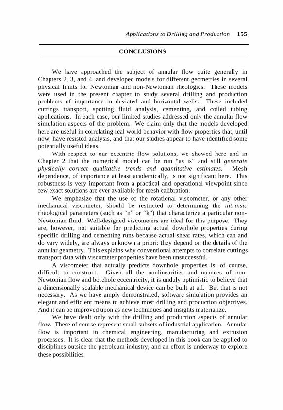
Applications to Drilling and Production 155
CONCLUSIONS
We have approached the subject of annular flow quite generally inChapters 2, 3, and 4, and developed models for different geometries in severalphysical limits for Newtonian and non-Newtonian rheologies. These modelswere used in the present chapter to study several drilling and productionproblems of importance in deviated and horizontal wells. These includedcuttings transport, spotting fluid analysis, cementing, and coiled tubingapplications. In each case, our limited studies addressed only the annular flowsimulation aspects of the problem. We claim only that the models developedhere are useful in correlating real world behavior with flow properties that, untilnow, have resisted analysis, and that our studies appear to have identified somepotentially useful ideas.
With respect to our eccentric flow solutions, we showed here and inChapter 2 that the numerical model can be run “as is” and still generatephysically correct qualitative trends and quantitative estimates. Meshdependence, of importance at least academically, is not significant here. Thisrobustness is very important from a practical and operational viewpoint sincefew exact solutions are ever available for mesh calibration.
We emphasize that the use of the rotational viscometer, or any othermechanical viscometer, should be restricted to determining the intrinsicrheological parameters (such as “n” or “k”) that characterize a particular non-Newtonian fluid. Well-designed viscometers are ideal for this purpose. Theyare, however, not suitable for predicting actual downhole properties duringspecific drilling and cementing runs because actual shear rates, which can anddo vary widely, are always unknown a priori: they depend on the details of theannular geometry. This explains why conventional attempts to correlate cuttingstransport data with viscometer properties have been unsuccessful.
A viscometer that actually predicts downhole properties is, of course,difficult to construct. Given all the nonlinearities and nuances of non-Newtonian flow and borehole eccentricity, it is unduly optimistic to believe thata dimensionally scalable mechanical device can be built at all. But that is notnecessary. As we have amply demonstrated, software simulation provides anelegant and efficient means to achieve most drilling and production objectives.And it can be improved upon as new techniques and insights materialize.
We have dealt only with the drilling and production aspects of annularflow. These of course represent small subsets of industrial application. Annularflow is important in chemical engineering, manufacturing and extrusionprocesses. It is clear that the methods developed in this book can be applied todisciplines outside the petroleum industry, and an effort is underway to explorethese possibilities.
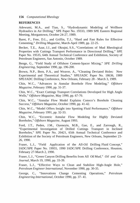
156 Computational Rheology
REFERENCES
Adewumi, M.A., and Tian, S., “Hydrodynamic Modeling of WellboreHydraulics in Air Drilling,” SPE Paper No. 19333, 1989 SPE Eastern RegionalMeeting, Morgantown, October 24-27, 1989.
Baret, F., Free, D.L., and Griffin, T.J., “Hard and Fast Rules for EffectiveCementing,” Drilling Magazine, March-April 1989, pp. 22-25.
Becker, T.E., Azar, J.J., and Okrajni, S.S., “Correlations of Mud RheologicalProperties with Cuttings Transport Performance in Directional Drilling,” SPEPaper No. 19535, 64th Annual Technical Conference and Exhibition, Society ofPetroleum Engineers, San Antonio, October 1989.
Benge, G., “Field Study of Offshore Cement-Spacer Mixing,” SPE DrillingEngineering, September 1990, pp. 196-200.
Brown, N.P., Bern, P.A., and Weaver, A., “Cleaning Deviated Holes: NewExperimental and Theoretical Studies,” SPE/IADC Paper No. 18636, 1989SPE/IADC Drilling Conference, New Orleans, February 28 - March 3, 1989.
Chin, W.C., “Advances in Annular Borehole Flow Modeling,” OffshoreMagazine, February 1990, pp. 31-37.
Chin, W.C., “Exact Cuttings Transport Correlations Developed for High AngleWells,” Offshore Magazine, May 1990, pp. 67-70.
Chin, W.C., “Annular Flow Model Explains Conoco’s Borehole CleaningSuccess,” Offshore Magazine, October 1990, pp. 41-42.
Chin, W.C., “Model Offers Insight into Spotting Fluid Performance,” OffshoreMagazine, February 1991, pp. 32-33.
Chin, W.C., “Eccentric Annular Flow Modeling for Highly DeviatedBoreholes,” Offshore Magazine, August 1993.
Ford, J.T., Peden, J.M., Oyeneyin, M.B., Gao, E., and Zarrough, R.,“Experimental Investigation of Drilled Cuttings Transport in InclinedBoreholes,” SPE Paper No. 20421, 65th Annual Technical Conference andExhibition of the Society of Petroleum Engineers, New Orleans, September 23-26, 1990.
Fraser, L.J., “Field Application of the All-Oil Drilling Fluid Concept,”IADC/SPE Paper No. 19955, 1990 IADC/SPE Drilling Conference, Houston,February 27-March 2, 1990.
Fraser, L.J., “Green Canyon Drilling Benefits from All Oil Mud,” Oil and GasJournal, March 19, 1990, pp. 33-39.
Fraser, L.J., “Effective Ways to Clean and Stabilize High-Angle Hole,”Petroleum Engineer International, November 1990, pp. 30-35.
George, C., “Innovations Change Cementing Operations,” PetroleumEngineering International, October 1990, pp. 37- 41.
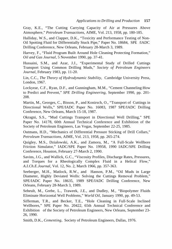
Applications to Drilling and Production 157
Gray, K.E., “The Cutting Carrying Capacity of Air at Pressures AboveAtmosphere,” Petroleum Transactions, AIME, Vol. 213, 1958, pp. 180-185.
Halliday, W.S., and Clapper, D.K., “Toxicity and Performance Testing of Non-Oil Spotting Fluid for Differentially Stuck Pipe,” Paper No. 18684, SPE /IADCDrilling Conference, New Orleans, February 28-March 3, 1989.
Harvey, F., “Fluid Program Built Around Hole Cleaning Protecting Formation,”Oil and Gas Journal, 5 November 1990, pp. 37-41.
Hussaini, S.M., and Azar, J.J., “Experimental Study of Drilled CuttingsTransport Using Common Drilling Muds,” Society of Petroleum EngineersJournal, February 1983, pp. 11-20.
Lin, C.C., The Theory of Hydrodynamic Stability, Cambridge University Press,London, 1967.
Lockyear, C.F., Ryan, D.F., and Gunningham, M.M., “Cement Channeling:Howto Predict and Prevent,” SPE Drilling Engineering, September 1990, pp. 201-208.
Martin, M., Georges, C., Bisson, P., and Konirsch, O., “Transport of Cuttings inDirectional Wells,” SPE/IADC Paper No. 16083, 1987 SPE/IADC DrillingConference, New Orleans, March 15-18, 1987.
Okragni, S.S., “Mud Cuttings Transport in Directional Well Drilling,” SPEPaper No. 14178, 60th Annual Technical Conference and Exhibition of theSociety of Petroleum Engineers, Las Vegas, September 22-25, 1985.
Outmans, H.D., “Mechanics of Differential Pressure Sticking of Drill Collars,”Petroleum Transactions, AIME, Vol. 213, 1958, pp. 265-274.
Quigley, M.S., Dzialowski, A.K., and Zamora, M., “A Full-Scale WellboreFriction Simulator,” IADC/SPE Paper No. 19958, 1990 IADC/SPE DrillingConference, Houston, February 27-March 2, 1990.
Savins, J.G., and Wallick, G.C., “Viscosity Profiles, Discharge Rates, Pressures,and Torques for a Rheologically Complex Fluid in a Helical Flow,”A.I.Ch.E.Journal, Vol. 12, No. 2, March 1966, pp. 357-363.
Seeberger, M.H., Matlock, R.W., and Hanson, P.M., “Oil Muds in LargeDiameter, Highly Deviated Wells: Solving the Cuttings Removal Problem,”SPE/IADC Paper No. 18635, 1989 SPE/IADC Drilling Conference, NewOrleans, February 28-March 3, 1989.
Seheult, M., Grebe, L., Traweek, J.E., and Dudley, M., “Biopolymer FluidsEliminate Horizontal Well Problems,” World Oil, January 1990, pp. 49-53.
Sifferman, T.R., and Becker, T.E., “Hole Cleaning in Full-Scale InclinedWellbores,” SPE Paper No. 20422, 65th Annual Technical Conference andExhibition of the Society of Petroleum Engineers, New Orleans, September 23-26, 1990.
Smith, D.K., Cementing, Society of Petroleum Engineers, Dallas, 1976.
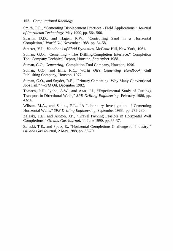
158 Computational Rheology
Smith, T.R., “Cementing Displacement Practices - Field Applications,” Journalof Petroleum Technology, May 1990, pp. 564-566.
Sparlin, D.D., and Hagen, R.W., “Controlling Sand in a HorizontalCompletion,” World Oil, November 1988, pp. 54-58.
Streeter, V.L., Handbook of Fluid Dynamics, McGraw-Hill, New York, 1961.
Suman, G.O., “Cementing - The Drilling/Completion Interface,” CompletionTool Company Technical Report, Houston, September 1988.
Suman, G.O., Cementing, Completion Tool Company, Houston, 1990.
Suman, G.O., and Ellis, R.C., World Oil's Cementing Handbook, GulfPublishing Company, Houston, 1977.
Suman, G.O., and Snyder, R.E., “Primary Cementing: Why Many ConventionalJobs Fail,” World Oil, December 1982.
Tomren, P.H., Iyoho, A.W., and Azar, J.J., “Experimental Study of CuttingsTransport in Directional Wells,” SPE Drilling Engineering, February 1986, pp.43-56.
Wilson, M.A., and Sabins, F.L., “A Laboratory Investigation of CementingHorizontal Wells,” SPE Drilling Engineering, September 1988, pp. 275-280.
Zaleski, T.E., and Ashton, J.P., “Gravel Packing Feasible in Horizontal WellCompletions,” Oil and Gas Journal, 11 June 1990, pp. 33-37.
Zaleski, T.E., and Spatz, E., “Horizontal Completions Challenge for Industry,”Oil and Gas Journal, 2 May 1988, pp. 58-70.
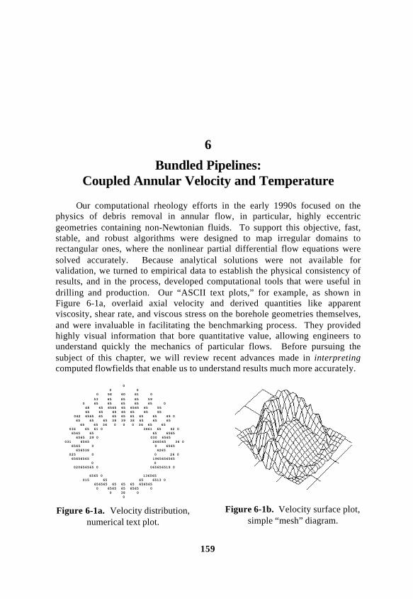
159
6
Bundled Pipelines:Coupled Annular Velocity and Temperature
Our computational rheology efforts in the early 1990s focused on thephysics of debris removal in annular flow, in particular, highly eccentricgeometries containing non-Newtonian fluids. To support this objective, fast,stable, and robust algorithms were designed to map irregular domains torectangular ones, where the nonlinear partial differential flow equations weresolved accurately. Because analytical solutions were not available forvalidation, we turned to empirical data to establish the physical consistency ofresults, and in the process, developed computational tools that were useful indrilling and production. Our “ASCII text plots,” for example, as shown inFigure 6-1a, overlaid axial velocity and derived quantities like apparentviscosity, shear rate, and viscous stress on the borehole geometries themselves,and were invaluable in facilitating the benchmarking process. They providedhighly visual information that bore quantitative value, allowing engineers tounderstand quickly the mechanics of particular flows. Before pursuing thesubject of this chapter, we will review recent advances made in interpretingcomputed flowfields that enable us to understand results much more accurately.
0 0 0 0 58 60 61 0
53 65 65 65 59 0 65 65 65 65 65 0 48 65 6565 65 6565 65 55 65 65 65 65 65 65 65 042 6565 65 65 65 65 65 65 49 0 65 65 65 38 39 38 65 65 65 65 65 36 0 0 0 36 65 65 036 65 61 0 3461 65 42 0 6565 65 65 6565 6565 29 0 030 6565 031 6565 266565 34 0 6565 0 0 6565 656538 4265 025 0 0 26 0 65656565 1965656565 0 0 020656565 0 065656519 0
6565 0 136565 015 65 65 6513 0 656565 65 65 65 656565 0 6565 65 6565 0 0 38 0 0
Figure 6-1a. Velocity distribution,numerical text plot.
Figure 6-1b. Velocity surface plot,simple “mesh” diagram.
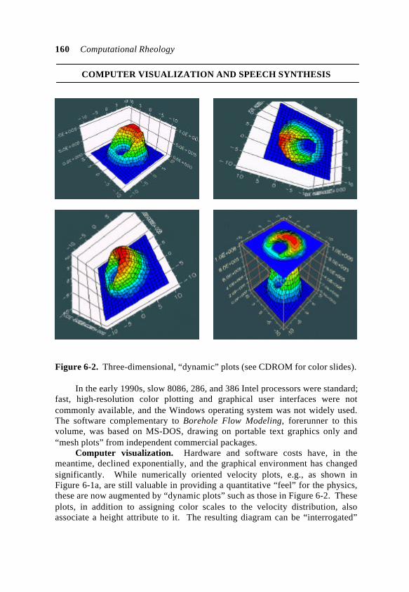
160 Computational Rheology
COMPUTER VISUALIZATION AND SPEECH SYNTHESIS
Figure 6-2. Three-dimensional, “dynamic” plots (see CDROM for color slides).
In the early 1990s, slow 8086, 286, and 386 Intel processors were standard;fast, high-resolution color plotting and graphical user interfaces were notcommonly available, and the Windows operating system was not widely used.The software complementary to Borehole Flow Modeling, forerunner to thisvolume, was based on MS-DOS, drawing on portable text graphics only and“mesh plots” from independent commercial packages.
Computer visualization. Hardware and software costs have, in themeantime, declined exponentially, and the graphical environment has changedsignificantly. While numerically oriented velocity plots, e.g., as shown inFigure 6-1a, are still valuable in providing a quantitative “feel” for the physics,these are now augmented by “dynamic plots” such as those in Figure 6-2. Theseplots, in addition to assigning color scales to the velocity distribution, alsoassociate a height attribute to it. The resulting diagram can be “interrogated”
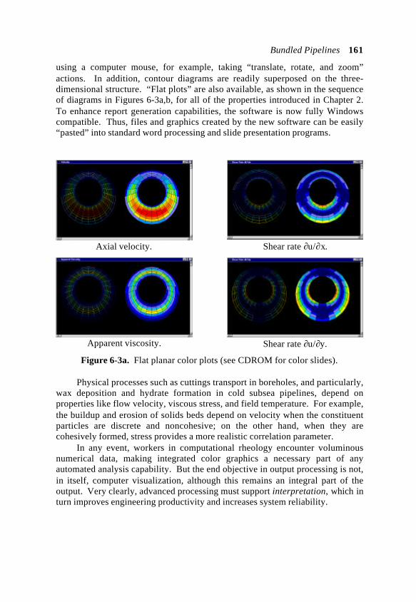
Bundled Pipelines 161
using a computer mouse, for example, taking “translate, rotate, and zoom”actions. In addition, contour diagrams are readily superposed on the three-dimensional structure. “Flat plots” are also available, as shown in the sequenceof diagrams in Figures 6-3a,b, for all of the properties introduced in Chapter 2.To enhance report generation capabilities, the software is now fully Windowscompatible. Thus, files and graphics created by the new software can be easily“pasted” into standard word processing and slide presentation programs.
Axial velocity.
Apparent viscosity.
Shear rate ∂u/∂x.
Shear rate ∂u/∂y.
Figure 6-3a. Flat planar color plots (see CDROM for color slides).
Physical processes such as cuttings transport in boreholes, and particularly,wax deposition and hydrate formation in cold subsea pipelines, depend onproperties like flow velocity, viscous stress, and field temperature. For example,the buildup and erosion of solids beds depend on velocity when the constituentparticles are discrete and noncohesive; on the other hand, when they arecohesively formed, stress provides a more realistic correlation parameter.
In any event, workers in computational rheology encounter voluminousnumerical data, making integrated color graphics a necessary part of anyautomated analysis capability. But the end objective in output processing is not,in itself, computer visualization, although this remains an integral part of theoutput. Very clearly, advanced processing must support interpretation, which inturn improves engineering productivity and increases system reliability.
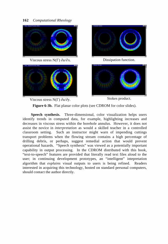
162 Computational Rheology
Viscous stress N(Γ) ∂u/∂x.
Viscous stress N(Γ) ∂u/∂y.
Dissipation function.
Stokes product.
Figure 6-3b. Flat planar color plots (see CDROM for color slides).
Speech synthesis. Three-dimensional, color visualization helps usersidentify trends in computed data, for example, highlighting increases anddecreases in viscous stress within the borehole annulus. However, it does notassist the novice in interpretation as would a skilled teacher in a controlledclassroom setting. Such an instructor might warn of impending cuttingstransport problems when the flowing stream contains a high percentage ofdrilling debris, or perhaps, suggest remedial action that would preventoperational hazards. “Speech synthesis” was viewed as a potentially importantcapability in output processing. In the CDROM distributed with this book,“text-to-speech” features are provided that literally read text files aloud to theuser; in continuing development prototypes, an “intelligent” intepretationalgorithm that explains visual outputs to users is being refined. Readersinterested in acquiring this technology, hosted on standard personal computers,should contact the author directly.
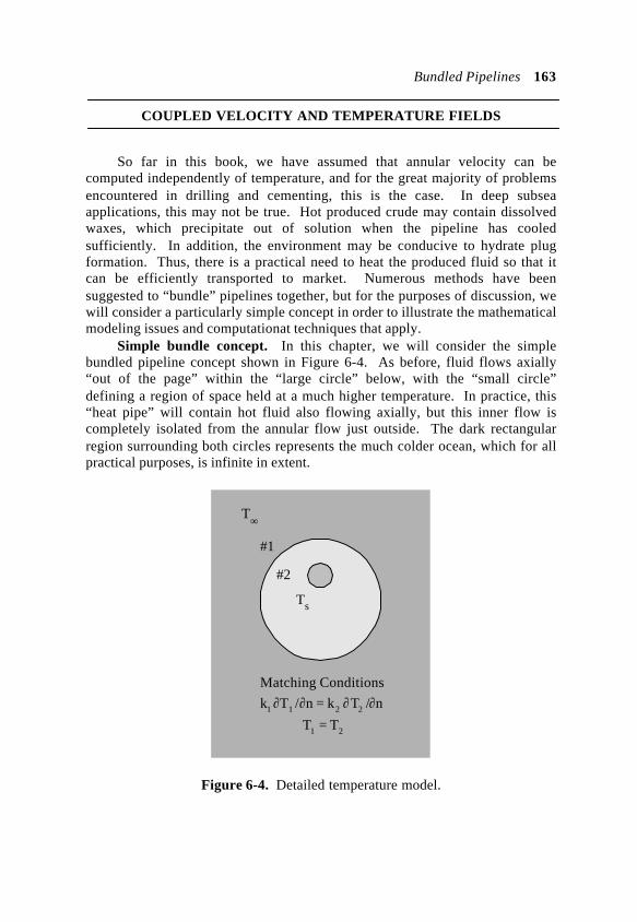
Bundled Pipelines 163
COUPLED VELOCITY AND TEMPERATURE FIELDS
So far in this book, we have assumed that annular velocity can becomputed independently of temperature, and for the great majority of problemsencountered in drilling and cementing, this is the case. In deep subseaapplications, this may not be true. Hot produced crude may contain dissolvedwaxes, which precipitate out of solution when the pipeline has cooledsufficiently. In addition, the environment may be conducive to hydrate plugformation. Thus, there is a practical need to heat the produced fluid so that itcan be efficiently transported to market. Numerous methods have beensuggested to “bundle” pipelines together, but for the purposes of discussion, wewill consider a particularly simple concept in order to illustrate the mathematicalmodeling issues and computationat techniques that apply.
Simple bundle concept. In this chapter, we will consider the simplebundled pipeline concept shown in Figure 6-4. As before, fluid flows axially“out of the page” within the “large circle” below, with the “small circle”defining a region of space held at a much higher temperature. In practice, this“heat pipe” will contain hot fluid also flowing axially, but this inner flow iscompletely isolated from the annular flow just outside. The dark rectangularregion surrounding both circles represents the much colder ocean, which for allpractical purposes, is infinite in extent.
T∞
k1 ∂T1 /∂n = k2 ∂T2 /∂n
T1 = T2
#1
#2
Ts
Matching Conditions
Figure 6-4. Detailed temperature model.
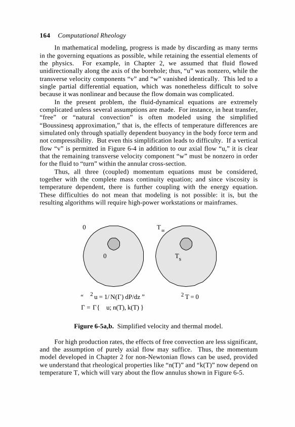
164 Computational Rheology
In mathematical modeling, progress is made by discarding as many termsin the governing equations as possible, while retaining the essential elements ofthe physics. For example, in Chapter 2, we assumed that fluid flowedunidirectionally along the axis of the borehole; thus, “u” was nonzero, while thetransverse velocity components “v” and “w” vanished identically. This led to asingle partial differential equation, which was nonetheless difficult to solvebecause it was nonlinear and because the flow domain was complicated.
In the present problem, the fluid-dynamical equations are extremelycomplicated unless several assumptions are made. For instance, in heat transfer,“free” or “natural convection” is often modeled using the simplified“Boussinesq approximation,” that is, the effects of temperature differences aresimulated only through spatially dependent buoyancy in the body force term andnot compressibility. But even this simplification leads to difficulty. If a verticalflow “v” is permitted in Figure 6-4 in addition to our axial flow “u,” it is clearthat the remaining transverse velocity component “w” must be nonzero in orderfor the fluid to “turn” within the annular cross-section.
Thus, all three (coupled) momentum equations must be considered,together with the complete mass continuity equation; and since viscosity istemperature dependent, there is further coupling with the energy equation.These difficulties do not mean that modeling is not possible: it is, but theresulting algorithms will require high-power workstations or mainframes.
∇2 T = 0
T∞
Ts
“ ∇2 u = 1/ Ν(Γ) dP/dz ”
0
0
Γ = Γ ∇u; n(T), k(T)
Figure 6-5a,b. Simplified velocity and thermal model.
For high production rates, the effects of free convection are less significant,and the assumption of purely axial flow may suffice. Thus, the momentummodel developed in Chapter 2 for non-Newtonian flows can be used, providedwe understand that rheological properties like “n(T)” and “k(T)” now depend ontemperature T, which will vary about the flow annulus shown in Figure 6-5.
Bundled Pipelines 165
The more complicated cross-sectional thermal boundary condition modelin Figure 6-4, which matches temperature and normal heat flux at the annulusand ocean interface, can be replaced by the simpler model shown at the right ofFigure 6-5. If, in the complete energy equation, we neglect changes in the axialdirection, transient effects, and internal heat generation, Laplace’s equation forT(y,x) arises in the simple limit of constant thermal properties. This leads to theelementary pipe bundle model summarized in Figure 6-5.
In this computational scheme, temperature is solved first, and stored as afunction of (y,x). Then, the flow solver developed in Chapter 2 is used, but “n”and “k” now vary with position. Importantly, both u(y,x) and T(y,x) are solvedby the same “boundary conforming, curvilinear mesh” algorithms developedpreviously since the governing equations are almost identical. Of course, morecomplicated physical flows do exist, which require more elaborate models; otherbundling concepts may involve multiple embedded pipes, resulting in annuliwith multiple “holes.” These extensions will be discussed later.
Design issues. If we assume that the pipeline is flowing under a fixedpressure gradient, that is, acting through reservoir pressure alone, it is clear thatunder isothermal conditions, the volume flow rate for the annulus in Figure 6-5ain general increases with increasing eccentricity, as demonstrated in Chapter 2.Of course, the temperature field T(y,x) in reality varies throughout, so that therheological properties of the fluid likewise vary. In general, n, k, and yieldstress, or other properties characterizing the constitutive relation, will depend ontemperature and wax content, in a manner that must be determined in thelaboratory. Once these relations are obtained, several design issues arise.
For example, the total revenue to the operator depends on the net volumeof fluid delivered; in this respect, qualitatively speaking, eccentricity is good.However, high eccentricity may imply that the surrounding fluid is notuniformly heated, so that waxes and hydrates form locally and possiblyprecipitate out of solution. Centralization of the heating pipe may suggest lessthroughput, in the sense that there is less eccentricity; bear in mind, though, thatincreased temperatures imply reduced viscosity, which lead to more efficientproduction. Thus, tradeoff studies are required, based on detailed simulation.Cost minimization should be planned at the outset. Fixed costs include thoseassociated with the sizes of inner and outer pipes, and the purchase of heatingsystems. Variable elements are related to energy costs, “down times” due to“plugging” or required maintenance, and so on. In general, it is clear that theeconomic optimization problem is very nonlinear, and must include the coupledvelocity and thermal simulator as an essential element.
Sample calculation. To illustrate the basic approach, we might consider aflowline having a given diameter, in one case containing a narrow heat pipe, andin the second, a wider one. Figure 6-6a shows the computed velocity field forthe narrow pipe, with high “red” velocities in the eccentric part of the annulus,while Figure 6-7a illustrates the analogous velocity result for the much wider
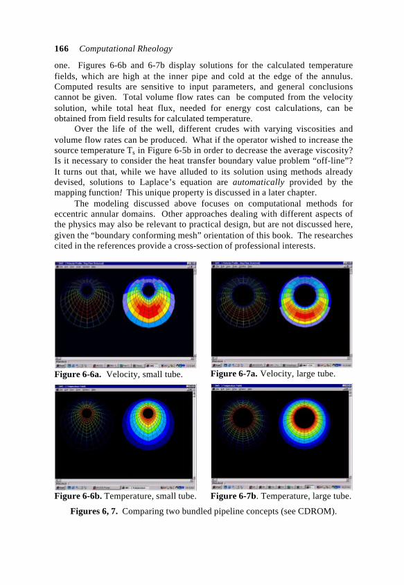
166 Computational Rheology
one. Figures 6-6b and 6-7b display solutions for the calculated temperaturefields, which are high at the inner pipe and cold at the edge of the annulus.Computed results are sensitive to input parameters, and general conclusionscannot be given. Total volume flow rates can be computed from the velocitysolution, while total heat flux, needed for energy cost calculations, can beobtained from field results for calculated temperature.
Over the life of the well, different crudes with varying viscosities andvolume flow rates can be produced. What if the operator wished to increase thesource temperature Ts in Figure 6-5b in order to decrease the average viscosity?Is it necessary to consider the heat transfer boundary value problem “off-line”?It turns out that, while we have alluded to its solution using methods alreadydevised, solutions to Laplace’s equation are automatically provided by themapping function! This unique property is discussed in a later chapter.
The modeling discussed above focuses on computational methods foreccentric annular domains. Other approaches dealing with different aspects ofthe physics may also be relevant to practical design, but are not discussed here,given the “boundary conforming mesh” orientation of this book. The researchescited in the references provide a cross-section of professional interests.
Figure 6-6a. Velocity, small tube.
Figure 6-6b. Temperature, small tube.
Figure 6-7a. Velocity, large tube.
Figure 6-7b. Temperature, large tube.
Figures 6, 7. Comparing two bundled pipeline concepts (see CDROM).
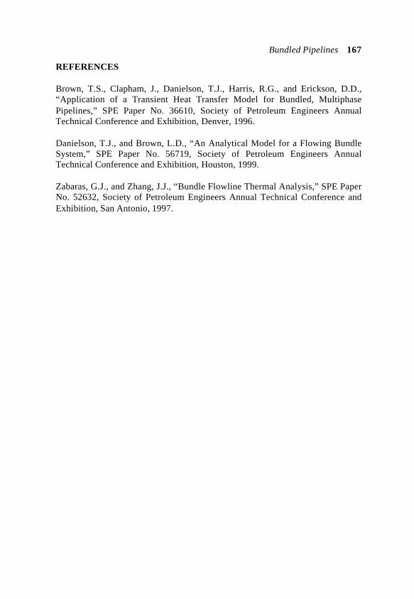
Bundled Pipelines 167
REFERENCES
Brown, T.S., Clapham, J., Danielson, T.J., Harris, R.G., and Erickson, D.D.,“Application of a Transient Heat Transfer Model for Bundled, MultiphasePipelines,” SPE Paper No. 36610, Society of Petroleum Engineers AnnualTechnical Conference and Exhibition, Denver, 1996.
Danielson, T.J., and Brown, L.D., “An Analytical Model for a Flowing BundleSystem,” SPE Paper No. 56719, Society of Petroleum Engineers AnnualTechnical Conference and Exhibition, Houston, 1999.
Zabaras, G.J., and Zhang, J.J., “Bundle Flowline Thermal Analysis,” SPE PaperNo. 52632, Society of Petroleum Engineers Annual Technical Conference andExhibition, San Antonio, 1997.
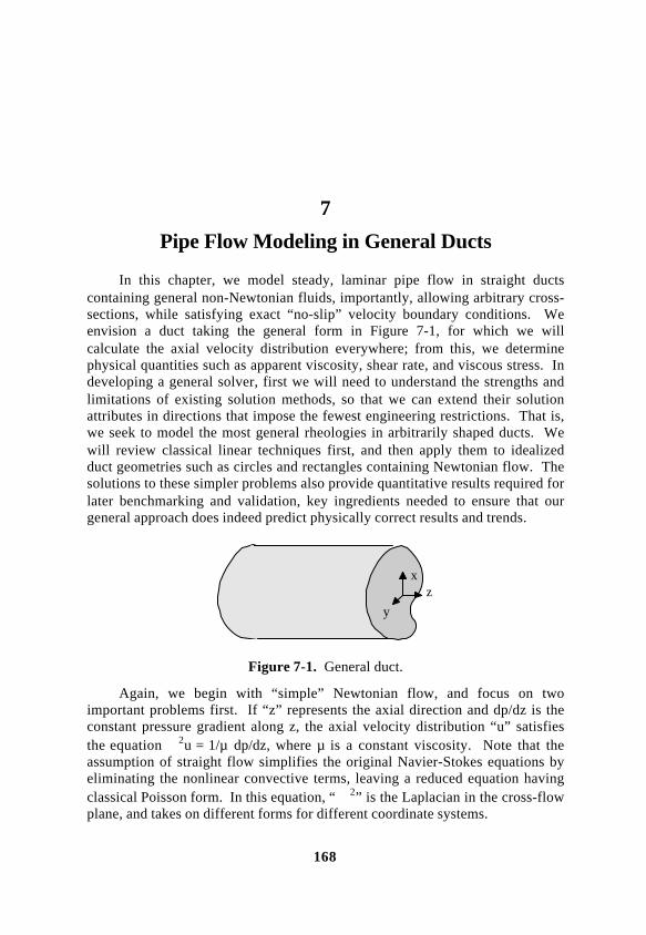
168
7
Pipe Flow Modeling in General Ducts
In this chapter, we model steady, laminar pipe flow in straight ductscontaining general non-Newtonian fluids, importantly, allowing arbitrary cross-sections, while satisfying exact “no-slip” velocity boundary conditions. Weenvision a duct taking the general form in Figure 7-1, for which we willcalculate the axial velocity distribution everywhere; from this, we determinephysical quantities such as apparent viscosity, shear rate, and viscous stress. Indeveloping a general solver, first we will need to understand the strengths andlimitations of existing solution methods, so that we can extend their solutionattributes in directions that impose the fewest engineering restrictions. That is,we seek to model the most general rheologies in arbitrarily shaped ducts. Wewill review classical linear techniques first, and then apply them to idealizedduct geometries such as circles and rectangles containing Newtonian flow. Thesolutions to these simpler problems also provide quantitative results required forlater benchmarking and validation, key ingredients needed to ensure that ourgeneral approach does indeed predict physically correct results and trends.
zx
y
Figure 7-1. General duct.
Again, we begin with “simple” Newtonian flow, and focus on twoimportant problems first. If “z” represents the axial direction and dp/dz is theconstant pressure gradient along z, the axial velocity distribution “u” satisfiesthe equation ∇
2u = 1/µ dp/dz, where µ is a constant viscosity. Note that theassumption of straight flow simplifies the original Navier-Stokes equations byeliminating the nonlinear convective terms, leaving a reduced equation havingclassical Poisson form. In this equation, “∇
2” is the Laplacian in the cross-flowplane, and takes on different forms for different coordinate systems.
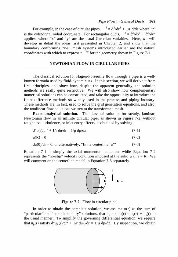
Pipe Flow in General Ducts 169
For example, in the case of circular pipes, ∇ 2 = d2/dr2 + 1/r d/dr where “r”
is the cylindrical radial coordinate. For rectangular ducts, ∇ 2 = ∂2/∂x2 + ∂2/∂y2
applies, where “x” and “y” are the usual Cartesian variables. Here, we willdevelop in detail the ideas first presented in Chapter 2, and show that theboundary conforming “r-s” mesh systems introduced earlier are the naturalcoordinates with which to express “∇
2” for the geometry shown in Figure 7-1.
NEWTONIAN FLOW IN CIRCULAR PIPES
The classical solution for Hagen-Poiseuille flow through a pipe is a well-known formula used by fluid-dynamicists. In this section, we will derive it fromfirst principles, and show how, despite the apparent generality, the solutionmethods are really quite restrictive. We will also show how complementarynumerical solutions can be constructed, and take the opportunity to introduce thefinite difference methods so widely used in the process and piping industry.These methods are, in fact, used to solve the grid generation equations, and also,the nonlinear flow equations written to the transformed mesh.
Exact analytical solution. The classical solution for steady, laminar,Newtonian flow in an infinite circular pipe, as shown in Figure 7-2, withoutroughness, turbulence, or inlet entry effects, is obtained by solving
d2u(r)/dr2 + 1/r du/dr = 1/µ dp/dz (7-1)
u(R) = 0 (7-2)
du(0)/dr = 0, or alternatively, “finite centerline ‘u’” (7-3)
Equation 7-1 is simply the axial momentum equation, while Equation 7-2represents the “no-slip” velocity condition imposed at the solid wall r = R. Wewill comment on the centerline model in Equation 7-3 separately.
r
z
Figure 7-2. Flow in circular pipe.
In order to obtain the complete solution, we assume u(r) as the sum of“particular” and “complementary” solutions, that is, take u(r) = up(r) + uc(r) inthe usual manner. To simplify the governing differential equation, we requirethat up(r) satisfy d2up (r)/dr2 + 1/r dup /dr = 1/µ dp/dz. By inspection, we obtain
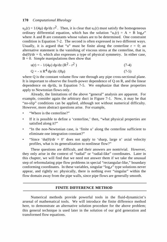
170 Computational Rheology
up(r) = 1/(4µ) dp/dz r2 . Then, it is clear that uc(r) must satisfy the homogeneousordinary differential equation, which has the solution “uc(r) = A + B loger”where A and B are constants whose values are to be determined. One constraintcondition is Equation 7-2. The second is often expressed in two different ways.Usually, it is argued that “u” must be finite along the centerline r = 0; analternative statement is the vanishing of viscous stress at the centerline, that is,du(0)/dr = 0, which also expresses a type of physical symmetry. In either case,B = 0. Simple manipulations then show that
u(r) = - 1/(4µ) dp/dz (R2 - r2 ) (7-4)
Q = - π R4 dp/dz /(8µ) (7-5)
where Q is the constant volume flow rate through any pipe cross-sectional plane.It is important to observe the fourth-power dependence of Q on R, and the lineardependence on dp/dz, in Equation 7-5. We emphasize that these propertiesapply to Newtonian flows only.
Already, the limitations of the above “general” analysis are apparent. Forexample, consider again the arbitrary duct in Figure 7-1. Now, it may be that“no-slip” conditions can be applied, although not without numerical difficulty.However, more abstract questions arise. For example,
• “Where is the centerline?”
• If it is possible to define a ‘centerline,’ then, “what physical properties aresatisfied along it?”
• “In the non-Newtonian case, is ‘finite u’ along the centerline sufficient toeliminate one integration constant?”
• “Since ‘du(0)/dr = 0’ does not apply to ‘sharp, large n’ axial velocityprofiles, what is its generalization to nonlinear flow?”
These questions are difficult, and their answers are nontrivial. However,they only arise in the context of “radial” or “radial-like” coordinates. Later inthis chapter, we will find that we need not answer them if we take the unusualstep of reformulating pipe flow problems in special “rectangular-like,” boundaryconforming coordinates. In these variables, singular “loger” type solutions neverappear, and rightly so: physically, there is nothing ever “singular” within theflow domain away from the pipe walls, since pipe flows are generally smooth.
FINITE DIFFERENCE METHOD
Numerical methods provide powerful tools in the fluid-dynamicist’sarsenal of mathematical tools. We will introduce the finite difference methodhere, to demonstrate an alternative solution procedure for the above problem;this general technique is used later in the solution of our grid generation andtransformed flow equations.

Pipe Flow in General Ducts 171
i-1 i i+1
i-1
i
i+1
r
u(r)
u
u
u A
B
Figure 7-3. Finite difference indexing.
Finite differences are easily explained using ideas from calculus. Theobjective, in this section, requires our replacement of Equation 7-1 by anequivalent system of algebraic equations, which is easily solved by standardmatrix methods. To accomplish this, we observe that the first derivatives atpoints “A” and “B” in Figure 7-3 are just du(A)/dr = (ui - ui-1)/∆r and du(B)/dr =(ui+1 - ui)/∆r, where ∆r is a constant mesh width, and “i” is an index used to marksuccessive divisions in r. Thus, the second derivative at “i” can be calculated as
d2u(ri )/dr2 = (du(B)/dr - du(A)/dr)/∆r= (ui-1 - 2ui + ui+1 )/(∆r)2 (7-6)
The first derivative at “i” appears more straightforwardly as
du(ri )/dr = (ui+1 - ui-1 )/(2∆r) (7-7)
If we now substitute Equations 7-6 and 7-7 in Equation 7-1, we obtain theresulting “central difference approximation”
(ui-1 - 2ui + ui+1) /(∆r)2 + (ui+1 - ui-1)/2ri∆r = (1/µ) dp/dz (7-8)
which can be rearranged to give
1- ∆r /(2ri )ui-1 + -2ui + 1+ ∆r /(2ri )ui+1 (7-9)
= (∆r)2/µ dp/dz
Equations 7-6 and 7-7 are “centrally” differenced because first and secondderivatives at “i” involve values both to the left and right. It can be shown thatcentral differences are more accurate than skewed “backward” or “forward”approximations; thus, for a fixed number of meshes, central differencingprovides the greatest accuracy. In the language of numerical analysis, centraldifference methods are “second order” accurate.
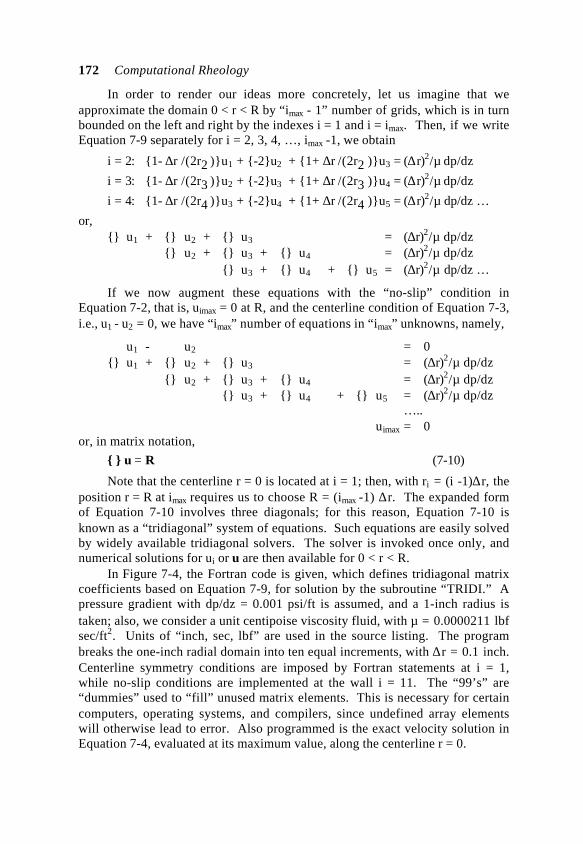
172 Computational Rheology
In order to render our ideas more concretely, let us imagine that weapproximate the domain 0 < r < R by “imax - 1” number of grids, which is in turnbounded on the left and right by the indexes i = 1 and i = imax. Then, if we writeEquation 7-9 separately for i = 2, 3, 4, …, imax -1, we obtain
i = 2: 1- ∆r /(2r2 )u1 + -2u2 + 1+ ∆r /(2r2 )u3 = (∆r)2/µ dp/dz
i = 3: 1- ∆r /(2r3 )u2 + -2u3 + 1+ ∆r /(2r3 )u4 = (∆r)2/µ dp/dz
i = 4: 1- ∆r /(2r4 )u3 + -2u4 + 1+ ∆r /(2r4 )u5 = (∆r)2/µ dp/dz …
or, u1 + u2 + u3 = (∆r)2/µ dp/dz
u2 + u3 + u4 = (∆r)2/µ dp/dz u3 + u4 + u5 = (∆r)2/µ dp/dz …
If we now augment these equations with the “no-slip” condition inEquation 7-2, that is, uimax = 0 at R, and the centerline condition of Equation 7-3,i.e., u1 - u2 = 0, we have “imax” number of equations in “imax” unknowns, namely,
u1 - u2 = 0 u1 + u2 + u3 = (∆r)2/µ dp/dz
u2 + u3 + u4 = (∆r)2/µ dp/dz u3 + u4 + u5 = (∆r)2/µ dp/dz
…..uimax = 0
or, in matrix notation,
u = R (7-10)
Note that the centerline r = 0 is located at i = 1; then, with ri = (i -1)∆r, theposition r = R at imax requires us to choose R = (imax -1) ∆r. The expanded formof Equation 7-10 involves three diagonals; for this reason, Equation 7-10 isknown as a “tridiagonal” system of equations. Such equations are easily solvedby widely available tridiagonal solvers. The solver is invoked once only, andnumerical solutions for ui or u are then available for 0 < r < R.
In Figure 7-4, the Fortran code is given, which defines tridiagonal matrixcoefficients based on Equation 7-9, for solution by the subroutine “TRIDI.” Apressure gradient with dp/dz = 0.001 psi/ft is assumed, and a 1-inch radius istaken; also, we consider a unit centipoise viscosity fluid, with µ = 0.0000211 lbfsec/ft2. Units of “inch, sec, lbf” are used in the source listing. The programbreaks the one-inch radial domain into ten equal increments, with ∆r = 0.1 inch.Centerline symmetry conditions are imposed by Fortran statements at i = 1,while no-slip conditions are implemented at the wall i = 11. The “99’s” are“dummies” used to “fill” unused matrix elements. This is necessary for certaincomputers, operating systems, and compilers, since undefined array elementswill otherwise lead to error. Also programmed is the exact velocity solution inEquation 7-4, evaluated at its maximum value, along the centerline r = 0.
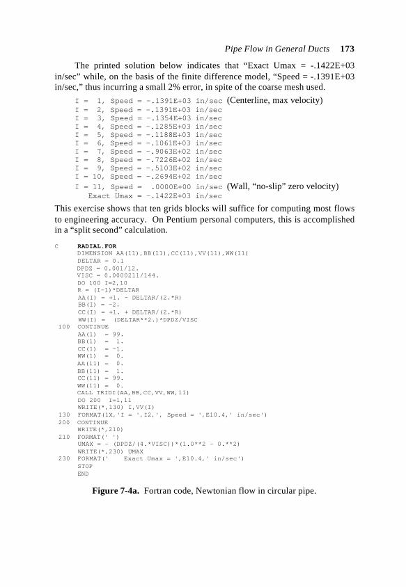
Pipe Flow in General Ducts 173
The printed solution below indicates that “Exact Umax = -.1422E+03in/sec” while, on the basis of the finite difference model, “Speed = -.1391E+03in/sec,” thus incurring a small 2% error, in spite of the coarse mesh used.
I = 1, Speed = -.1391E+03 in/sec (Centerline, max velocity)I = 2, Speed = -.1391E+03 in/secI = 3, Speed = -.1354E+03 in/secI = 4, Speed = -.1285E+03 in/secI = 5, Speed = -.1188E+03 in/secI = 6, Speed = -.1061E+03 in/secI = 7, Speed = -.9063E+02 in/secI = 8, Speed = -.7226E+02 in/secI = 9, Speed = -.5103E+02 in/secI = 10, Speed = -.2694E+02 in/sec
I = 11, Speed = .0000E+00 in/sec (Wall, “no-slip” zero velocity) Exact Umax = -.1422E+03 in/sec
This exercise shows that ten grids blocks will suffice for computing most flowsto engineering accuracy. On Pentium personal computers, this is accomplishedin a “split second” calculation.
C RADIAL.FOR DIMENSION AA(11),BB(11),CC(11),VV(11),WW(11) DELTAR = 0.1 DPDZ = 0.001/12. VISC = 0.0000211/144. DO 100 I=2,10 R = (I-1)*DELTAR AA(I) = +1. - DELTAR/(2.*R) BB(I) = -2. CC(I) = +1. + DELTAR/(2.*R) WW(I) = (DELTAR**2.)*DPDZ/VISC 100 CONTINUE AA(1) = 99. BB(1) = 1. CC(1) = -1. WW(1) = 0. AA(11) = 0. BB(11) = 1. CC(11) = 99. WW(11) = 0. CALL TRIDI(AA,BB,CC,VV,WW,11) DO 200 I=1,11 WRITE(*,130) I,VV(I) 130 FORMAT(1X,'I = ',I2,', Speed = ',E10.4,' in/sec') 200 CONTINUE WRITE(*,210) 210 FORMAT(' ') UMAX = - (DPDZ/(4.*VISC))*(1.0**2 - 0.**2) WRITE(*,230) UMAX 230 FORMAT(' Exact Umax = ',E10.4,' in/sec') STOP END
Figure 7-4a. Fortran code, Newtonian flow in circular pipe.
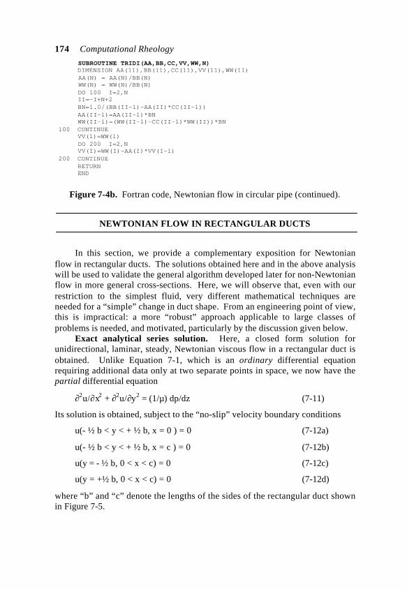
174 Computational Rheology
SUBROUTINE TRIDI(AA,BB,CC,VV,WW,N) DIMENSION AA(11),BB(11),CC(11),VV(11),WW(11) AA(N) = AA(N)/BB(N) WW(N) = WW(N)/BB(N) DO 100 I=2,N II=-I+N+2 BN=1.0/(BB(II-1)-AA(II)*CC(II-1)) AA(II-1)=AA(II-1)*BN WW(II-1)=(WW(II-1)-CC(II-1)*WW(II))*BN 100 CONTINUE VV(1)=WW(1) DO 200 I=2,N VV(I)=WW(I)-AA(I)*VV(I-1) 200 CONTINUE RETURN END
Figure 7-4b. Fortran code, Newtonian flow in circular pipe (continued).
NEWTONIAN FLOW IN RECTANGULAR DUCTS
In this section, we provide a complementary exposition for Newtonianflow in rectangular ducts. The solutions obtained here and in the above analysiswill be used to validate the general algorithm developed later for non-Newtonianflow in more general cross-sections. Here, we will observe that, even with ourrestriction to the simplest fluid, very different mathematical techniques areneeded for a “simple” change in duct shape. From an engineering point of view,this is impractical: a more “robust” approach applicable to large classes ofproblems is needed, and motivated, particularly by the discussion given below.
Exact analytical series solution. Here, a closed form solution forunidirectional, laminar, steady, Newtonian viscous flow in a rectangular duct isobtained. Unlike Equation 7-1, which is an ordinary differential equationrequiring additional data only at two separate points in space, we now have thepartial differential equation
∂2u/∂x2 + ∂2u/∂y2 = (1/µ) dp/dz (7-11)
Its solution is obtained, subject to the “no-slip” velocity boundary conditions
u(- ½ b < y < + ½ b, x = 0 ) = 0 (7-12a)
u(- ½ b < y < + ½ b, x = c ) = 0 (7-12b)
u(y = - ½ b, 0 < x < c) = 0 (7-12c)
u(y = +½ b, 0 < x < c) = 0 (7-12d)
where “b” and “c” denote the lengths of the sides of the rectangular duct shownin Figure 7-5.
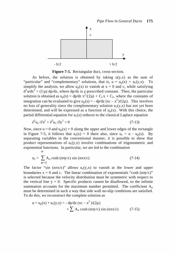
Pipe Flow in General Ducts 175
y
x
- b/2 + b/2
c
Figure 7-5. Rectangular duct, cross-section.
As before, the solution is obtained by taking u(y,x) as the sum of“particular” and “complementary” solutions, that is, u = up(x) + uc(y,x). Tosimplify the analysis, we allow up(x) to vanish at x = 0 and c, while satisfyingd2u/dx2 = (1/µ) dp/dz, where dp/dz is a prescribed constant. Then, the particularsolution is obtained as up(x) = dp/dz x2/(2µ) + C1 x + C2, where the constants ofintegration can be evaluated to give up(x) = - dp/dz (xc – x2 )/(2µ). This involvesno loss of generality since the complementary solution uc(y,x) has not yet beendetermined, and will be expressed as a function of up(x). With this choice, thepartial differential equation for uc(x) reduces to the classical Laplace equation
∂2uc /∂x2 + ∂2uc /∂y2 = 0 (7-13)
Now, since u = 0 and up(x) = 0 along the upper and lower edges of the rectanglein Figure 7-5, it follows that uc(x) = 0 there also, since uc = u - up(x). Byseparating variables in the conventional manner, it is possible to show thatproduct representations of uc(y,x) involve combinations of trigonometric andexponential functions. In particular, we are led to the combination
∞
uc = ∑ An cosh (nπy/c) sin (nπx/c) (7-14)n=1
The factor “sin (nπx/c)” allows uc(y,x) to vanish at the lower and upperboundaries x = 0 and c. The linear combination of exponentials “cosh (nπy/c)”is selected because the velocity distribution must be symmetric with respect tothe vertical line y = 0. Specific products cannot be disallowed, so the infinitesummation accounts for the maximum number permitted. The coefficient An
must be determined in such a way that side wall no-slip conditions are satisfied.To do this, we reconstruct the complete solution as
u = up(x) + uc(y,x) = - dp/dz (xc – x2 )/(2µ)
+ ∑ An cosh (nπy/c) sin (nπx/c) (7-15)
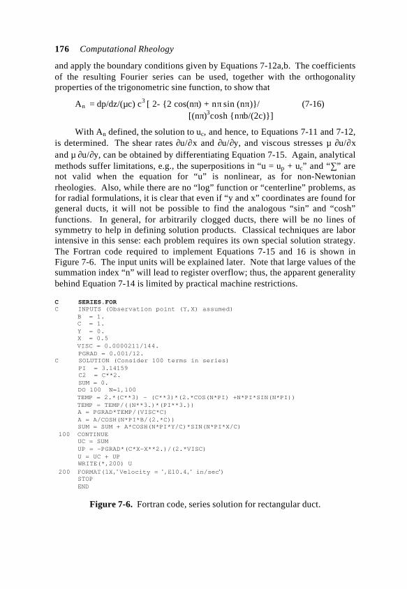
176 Computational Rheology
and apply the boundary conditions given by Equations 7-12a,b. The coefficientsof the resulting Fourier series can be used, together with the orthogonalityproperties of the trigonometric sine function, to show that
An = dp/dz/(µc) c3 [ 2- 2 cos(nπ) + nπ sin (nπ)/ (7-16)[(nπ)3cosh nπb/(2c)]
With An defined, the solution to uc, and hence, to Equations 7-11 and 7-12,is determined. The shear rates ∂u/∂x and ∂u/∂y, and viscous stresses µ ∂u/∂xand µ ∂u/∂y, can be obtained by differentiating Equation 7-15. Again, analyticalmethods suffer limitations, e.g., the superpositions in “u = up + uc” and “∑” arenot valid when the equation for “u” is nonlinear, as for non-Newtonianrheologies. Also, while there are no “log” function or “centerline” problems, asfor radial formulations, it is clear that even if “y and x” coordinates are found forgeneral ducts, it will not be possible to find the analogous “sin” and “cosh”functions. In general, for arbitrarily clogged ducts, there will be no lines ofsymmetry to help in defining solution products. Classical techniques are laborintensive in this sense: each problem requires its own special solution strategy.The Fortran code required to implement Equations 7-15 and 16 is shown inFigure 7-6. The input units will be explained later. Note that large values of thesummation index “n” will lead to register overflow; thus, the apparent generalitybehind Equation 7-14 is limited by practical machine restrictions.
C SERIES.FORC INPUTS (Observation point (Y,X) assumed) B = 1. C = 1. Y = 0. X = 0.5 VISC = 0.0000211/144. PGRAD = 0.001/12.C SOLUTION (Consider 100 terms in series) PI = 3.14159 C2 = C**2. SUM = 0. DO 100 N=1,100 TEMP = 2.*(C**3) - (C**3)*(2.*COS(N*PI) +N*PI*SIN(N*PI)) TEMP = TEMP/((N**3.)*(PI**3.)) A = PGRAD*TEMP/(VISC*C) A = A/COSH(N*PI*B/(2.*C)) SUM = SUM + A*COSH(N*PI*Y/C)*SIN(N*PI*X/C) 100 CONTINUE UC = SUM UP = -PGRAD*(C*X-X**2.)/(2.*VISC) U = UC + UP WRITE(*,200) U
200 FORMAT(1X,' Velocity = ',E10.4,' in/sec') STOP END
Figure 7-6. Fortran code, series solution for rectangular duct.
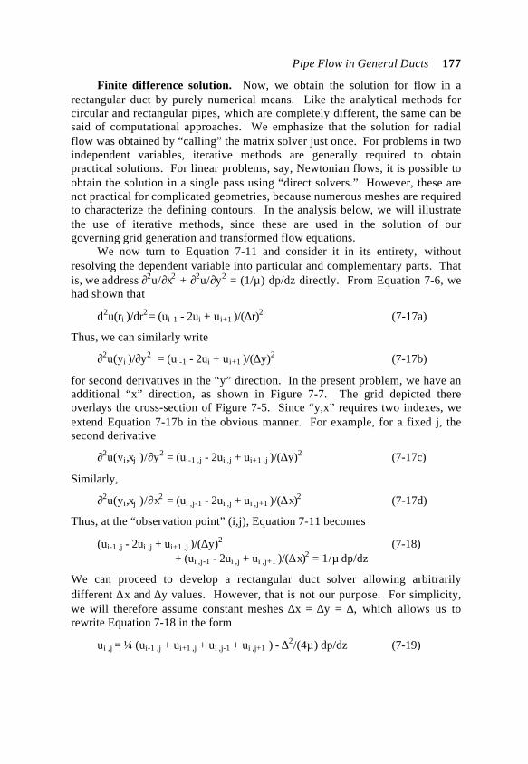
Pipe Flow in General Ducts 177
Finite difference solution. Now, we obtain the solution for flow in arectangular duct by purely numerical means. Like the analytical methods forcircular and rectangular pipes, which are completely different, the same can besaid of computational approaches. We emphasize that the solution for radialflow was obtained by “calling” the matrix solver just once. For problems in twoindependent variables, iterative methods are generally required to obtainpractical solutions. For linear problems, say, Newtonian flows, it is possible toobtain the solution in a single pass using “direct solvers.” However, these arenot practical for complicated geometries, because numerous meshes are requiredto characterize the defining contours. In the analysis below, we will illustratethe use of iterative methods, since these are used in the solution of ourgoverning grid generation and transformed flow equations.
We now turn to Equation 7-11 and consider it in its entirety, withoutresolving the dependent variable into particular and complementary parts. Thatis, we address ∂2u/∂x2 + ∂2u/∂y2 = (1/µ) dp/dz directly. From Equation 7-6, wehad shown that
d2u(ri )/dr2 = (ui-1 - 2ui + ui+1 )/(∆r)2 (7-17a)
Thus, we can similarly write
∂2u(yi )/∂y2 = (ui-1 - 2ui + ui+1 )/(∆y)2 (7-17b)
for second derivatives in the “y” direction. In the present problem, we have anadditional “x” direction, as shown in Figure 7-7. The grid depicted thereoverlays the cross-section of Figure 7-5. Since “y,x” requires two indexes, weextend Equation 7-17b in the obvious manner. For example, for a fixed j, thesecond derivative
∂2u(yi,xj )/∂y2 = (ui-1 ,j - 2ui ,j + ui+1 ,j )/(∆y)2 (7-17c)
Similarly,
∂2u(yi,xj )/∂x2 = (ui ,j-1 - 2ui ,j + ui ,j+1 )/(∆x)2 (7-17d)
Thus, at the “observation point” (i,j), Equation 7-11 becomes
(ui-1 ,j - 2ui ,j + ui+1 ,j )/(∆y)2 (7-18)+ (ui ,j-1 - 2ui ,j + ui ,j+1 )/(∆x)2 = 1/µ dp/dz
We can proceed to develop a rectangular duct solver allowing arbitrarilydifferent ∆x and ∆y values. However, that is not our purpose. For simplicity,we will therefore assume constant meshes ∆x = ∆y = ∆, which allows us torewrite Equation 7-18 in the form
ui ,j = ¼ (ui-1 ,j + ui+1 ,j + ui ,j-1 + ui ,j+1 ) - ∆2/(4µ) dp/dz (7-19)
178 Computational Rheology
y
x
∆
∆
i-1 i i+1
j
j-1
j+1
(i,j)
Figure 7-7. Rectangular finite difference grid.
Equation 7-19 is a central difference approximation to governing Equation7-11, which is second-order accurate. Interestingly, it can be used as a“recursion formula” that iteratively produces improved numerical solutions. Forexample, suppose that some approximate solution for u(i,j) is available. Then,an improved (left side) solution can be generated by evaluating the right side ofEquation 7-19 with it. It can be shown that, if this method converges, it willtend to the correct physical solution whatever the starting guess. Thus, if aninitial approximation were not available, a trivial “zero solution” for u would beperfectly acceptable! Such methods are known as “relaxation methods.” Sincewe have calculated improvements point-by-point (e.g., as opposed to an entireline of points at a time), the method used is a “point relaxation” method.
The Fortran source code implementing Equation 7-19 and the boundaryconditions in Equations 7-12a,b,c,d is given in Figure 7-8. The units used areidentical to those of the previous example, but here, a square duct having one-inch sides is considered. A mesh width of 0.1 inch is assumed, so that ten gridsare taken along each side of the square. Loop 100 initializes the “starting guess”for U(I,J) to zero, also setting vanishing velocities along the duct walls I = 1 and11, and J = 1 and 11. Loop 300 updates U(I,J) in the internal flow domainbounded by I = 2,…, 10 and J = 2, …, 10. One hundred iterations are taken,which more than converges the calculation; in a more refined implementation,suitable convergence criteria would be defined. “Q” provides the volume flowrate in gallons per minute, while “U” is calculated in inches per second. For theFortran code shown, computations are completed in less than one second, onPentium class personal computers.
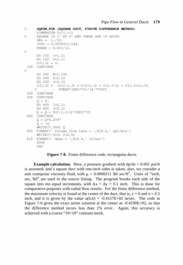
Pipe Flow in General Ducts 179
C SQFDM.FOR (SQUARE DUCT, FINITE DIFFERENCE METHOD) DIMENSION U(11,11)C SQUARE IS 1" BY 1" AND THERE ARE 10 GRIDS DEL = 1./10. VISC = 0.0000211/144. PGRAD = 0.001/12.C DO 100 I=1,11 DO 100 J=1,11 U(I,J) = 0. 100 CONTINUEC DO 300 N=1,100 DO 200 I=2,10 DO 200 J=2,10 U(I,J) = (U(I-1,J) + U(I+1,J) + U(I,J-1) + U(I,J+1))/4. 1 - PGRAD*(DEL**2)/(4.*VISC) 200 CONTINUE 300 CONTINUE Q = 0. DO 400 I=2,11 DO 400 J=2,11 Q = Q + U(I-1,J-1)*(DEL**2) 400 CONTINUE Q = Q*0.2597 Q = -Q WRITE(*,500) Q 500 FORMAT(' Volume flow rate = ',E10.4,' gal/min') WRITE(*,510) U(6,6) 510 FORMAT(' Umax = ',E10.4,' in/sec') STOP END
Figure 7-8. Finite difference code, rectangular ducts.
Example calculation. Here, a pressure gradient with dp/dz = 0.001 psi/ftis assumed, and a square duct with one-inch sides is taken; also, we consider aunit centipoise viscosity fluid, with µ = 0.0000211 lbf sec/ft2. Units of “inch,sec, lbf” are used in the source listing. The program breaks each side of thesquare into ten equal increments, with ∆x = ∆y = 0.1 inch. This is done forcomparative purposes with radial flow results. For the finite difference method,the maximum velocity is found at the center of the duct, that is, y = 0 and x = 0.5inch, and it is given by the value u(6,6) = -0.4157E+02 in/sec. The code inFigure 7-6 gives the exact series solution at the center as -0.4190E+02, so thatthe difference method incurs less than 1% error. Again, this accuracy isachieved with a coarse “10×10” constant mesh.
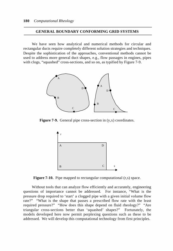
180 Computational Rheology
GENERAL BOUNDARY CONFORMING GRID SYSTEMS
We have seen how analytical and numerical methods for circular andrectangular ducts require completely different solution strategies and techniques.Despite the sophistication of the approaches, conventional methods cannot beused to address more general duct shapes, e.g., flow passages in engines, pipeswith clogs, “squashed” cross-sections, and so on, as typified by Figure 7-9.
A
B
A
B
C
DD
C
Figure 7-9. General pipe cross-section in (y,x) coordinates.
DA
B C
r
s
Figure 7-10. Pipe mapped to rectangular computational (r,s) space.
Without tools that can analyze flow efficiently and accurately, engineeringquestions of importance cannot be addressed. For instance, “What is thepressure drop required to ‘start’ a clogged pipe with a given initial volume flowrate?” “What is the shape that passes a prescribed flow rate with the leastrequired pressure?” “How does this shape depend on fluid rheology?” “Aretriangular cross-sections better than ‘squashed’ shapes?” Fortunately, themodels developed here now permit perplexing questions such as these to beaddressed. We will develop this computational technology from first principles.
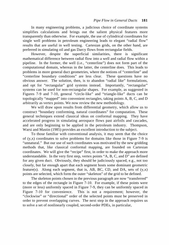
Pipe Flow in General Ducts 181
In many engineering problems, a judicious choice of coordinate systemssimplifies calculations and brings out the salient physical features moretransparently than otherwise. For example, the use of cylindrical coordinates forsingle well problems in petroleum engineering leads to elegant “radial flow”results that are useful in well testing. Cartesian grids, on the other hand, arepreferred in simulating oil and gas Darcy flows from rectangular fields.
However, despite the superficial similarities, there is significantmathematical difference between radial flow into a well and radial flow within apipeline. In the former, the well (i.e., “centerline”) does not form part of thecomputational domain, whereas in the latter, the centerline does. This leads toproblems in more general duct geometries, where the notions of “centerline” and“centerline boundary conditions” are less clear. These questions have noobvious answer. The solution, then, is to abandon “radial like” formulations,and opt for “rectangular” grid systems instead. Importantly, “rectangular”systems can be used for non-rectangular shapes. For example, as suggested inFigures 7-9 and 7-10, general “circle-like” and “triangle-like” ducts can betopologically “mapped” into convenient rectangles, taking points A, B, C, and Darbitrarily as vertex points. We now review the new methodology.
We will draw upon results from differential geometry, which allow us toconstruct “boundary conforming, natural coordinates” for computation. Thesegeneral techniques extend classical ideas on conformal mapping. They haveaccelerated progress in simulating aerospace flows past airfoils and cascades,and are only beginning to be applied in the petroleum industry. Thompson,Warsi and Mastin (1985) provides an excellent introduction to the subject.
To those familiar with conventional analysis, it may seem that the choiceof (y,x) coordinates to solve problems for domains like those in Figure 7-9 is“unnatural.” But our use of such coordinates was motivated by the new griddingmethods that, like classical conformal mapping, are founded on Cartesiancoordinates. We will give the “recipe” first, in order to make the approach moreunderstandable. In the very first step, vertex points “A, B, C, and D” are definedfor any given duct. Obviously, they should be judiciously spaced, e.g., not tooclosely, but far enough apart that each segment hosts some dominant geometricfeature(s). Along each segment, that is, AB, BC, CD, and DA, sets of (y,x)points are selected, which form the outer “skeleton” of the grid to be defined.
The skeleton points chosen in the previous paragraph are now “transferred”to the edges of the rectangle in Figure 7-10. For example, if these points were(more or less) uniformly spaced in Figure 7-9, they can be uniformly spaced inFigure 7-10 for convenience. This is not a requirement; however, the“clockwise” or “directional” order of the selected points must be preserved inorder to prevent overlapping curves. The next step in the approach requires usto solve a set of nonlinearly coupled, second-order PDEs, in particular,
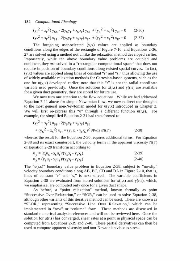
182 Computational Rheology
(yr2 + xr
2) yss - 2(ysyr + xs xr) ysr + (ys2 + xs
2) yrr = 0 (2-36)
(yr2 + xr
2) xss - 2(ysyr + xs xr) xsr + (ys2 + xs
2) xrr = 0 (2-37)
The foregoing user-selected (y,x) values are applied as boundaryconditions along the edges of the rectangle of Figure 7-10, and Equations 2-36,27 are solved using a method not unlike the relaxation method developed earlier.Importantly, while the above boundary value problems are coupled andnonlinear, they are solved in a “rectangular computational space” that does notrequire imposition of boundary conditions along twisted spatial curves. In fact,(y,x) values are applied along lines of constant “r” and “s,” thus allowing the useof widely available relaxation methods for Cartesian-based systems, such as theone for u(y,x) developed earlier; note that this “r” is not the radial coordinatevariable used previously. Once the solutions for x(r,s) and y(r,s) are availablefor a given duct geometry, they are stored for future use.
We now turn our attention to the flow equations. While we had addressedEquation 7-11 above for simple Newtonian flow, we now redirect our thoughtsto the most general non-Newtonian model for u(y,x) introduced in Chapter 2.We will first re-express this “u” through a different function u(r,s). Forexample, the simplified Equation 2-31 had transformed to
(yr2 + xr
2) uss - 2(ysyr + xs xr) usr
+ (ys2 + xs
2) urr = (ys xr - yrxs )2 ∂P/∂z /N(Γ) (2-38)
whereas the result for the Equation 2-30 requires additional terms. For Equation2-38 and its exact counterpart, the velocity terms in the apparent viscosity N(Γ)of Equation 2-29 transform according to
uy = (xrus - xsur)/(ysxr - yrxs) (2-39)
ux = (ysur - yrus)/(ysxr - yrxs) (2-40)
The “u(r,s)” boundary value problem in Equation 2-38, subject to “no-slip”velocity boundary conditions along AB, BC, CD and DA in Figure 7-10, that is,lines of constant “r” and “s,” is next solved. The variable coefficients inEquation 2-38 are evaluated from stored solutions for x(r,s) and y(r,s), which,we emphasize, are computed only once for a given duct shape.
As before, a “point relaxation” method, known formally as point“Successive Over Relaxation,” or “SOR,” can be used to solve Equation 2-38,although other variants of this iterative method can be used. These are known as“SLOR,” representing “Successive Line Over Relaxation,” which can beimplemented in “row” or “column” form. These methods are discussed instandard numerical analysis references and will not be reviewed here. Once thesolution for u(r,s) has converged, shear rates at a point in physical space can becomputed from Equations 2-39 and 2-40. These partial derivatives can then beused to compute apparent viscosity and non-Newtonian viscous stress.
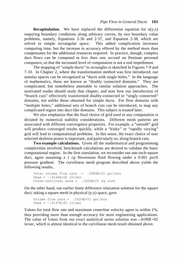
Pipe Flow in General Ducts 183
Recapitulation. We have replaced the differential equation for u(y,x)requiring boundary conditions along arbitrary curves, by two boundary valueproblems, namely, Equations 2-36 and 2-37, and Equation 2-38, which aresolved in simple rectangular space. This added complication increasescomputing time, but the increase in accuracy offered by the method more thancompensates for the additional resources required. In practice, though, complexduct flows can be computed in less than one second on Pentium personalcomputers, so that the increased level of computation is not a real impediment.
The mapping of “simple ducts” to rectangles is sketched In Figures 7-9 and7-10. In Chapter 2, where the transformation method was first introduced, ourannular spaces can be recognized as “ducts with single holes.” In the languageof mathematics, these are known as “doubly connected domains.” They arecomplicated, but nonetheless amenable to similar solution approaches. Themotivated reader should study that chapter, and note how our introduction of“branch cuts” effectively transformed doubly-connected to “singly connected”domains, not unlike those obtained for simple ducts. For flow domains with“multiple holes,” additional sets of branch cuts can be introduced, to map anycomplicated region into duct-like domains. This subject is treated later.
We also emphasize that the final choice of grid used in any computation isdictated by numerical stability considerations. Different mesh patterns areassociated with different convergence properties. For example, a “smooth” gridwill produce converged results quickly, while a “kinky” or “rapidly varying”grid will lead to computational problems. In this sense, the exact choice of userselected skeleton points is important, and particularly so, along branch cuts.
Two example calculations. Given all the mathematical and programmingcomplexities involved, benchmark calculations are desired to validate the basiccomputational engine. In the first simulation, we reconsider our one-inch-squareduct, again assuming a 1 cp Newtonian fluid flowing under a 0.001 psi/ftpressure gradient. The curvilinear mesh program described above yields thefollowing results,
Total volume flow rate = .5088E+01 gal/minUmax = -.4166E+02 in/secCross-sectional area = .1000E+01 sq inch
On the other hand, our earlier finite difference relaxation solution for the squareduct, taking a square mesh in physical (y,x) space, gave
Volume flow rate = .5026E+01 gal/minUmax = -.4157E+02 in/sec
Values for total flow rate and maximum centerline velocity agree to within 1%,thus providing more than enough accuracy for most engineering applications.The value of Umax from our exact analytical series solution was -.4190E+02in/sec, which is almost identical to the curvilinear mesh result obtained above.
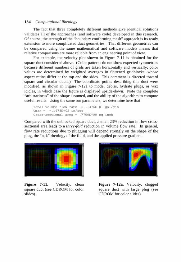
184 Computational Rheology
The fact that three completely different methods give identical solutionsvalidates all of the approaches (and software code) developed in this research.Of course, the strength of the “boundary conforming mesh” approach is its readyextension to more complicated duct geometries. That different geometries canbe compared using the same mathematical and software models means thatrelative comparisons are more reliable from an engineering point of view.
For example, the velocity plot shown in Figure 7-11 is obtained for thesquare duct considered above. (Color patterns do not show expected symmetriesbecause different numbers of grids are taken horizontally and vertically; colorvalues are determined by weighted averages in flattened gridblocks, whoseaspect ratios differ at the top and the sides. This comment is directed towardsquare and circular ducts.) The coordinate points describing this duct weremodified, as shown in Figure 7-12a to model debris, hydrate plugs, or waxicicles, in which case the figure is displayed upside-down. Note the complete“arbitrariness” of the shape assumed, and the ability of the algorithm to computeuseful results. Using the same run parameters, we determine here that
Total volume flow rate = .1476E+01 gal/minUmax = -.1473E+02 in/secCross-sectional area = .7700E+00 sq inch
Compared with the unblocked square duct, a small 23% reduction in flow cross-sectional area leads to a three-fold reduction in volume flow rate! In general,flow rate reductions due to plugging will depend strongly on the shape of theplug, the “n, k” rheology of the fluid, and the applied pressure gradient.
Figure 7-11. Velocity, cleansquare duct (see CDROM for colorslides).
Figure 7-12a. Velocity, cloggedsquare duct with large plug (seeCDROM for color slides).
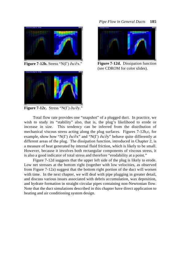
Pipe Flow in General Ducts 185
Figure 7-12b. Stress “N(Γ) ∂u/∂x.”
Figure 7-12c. Stress “N(Γ) ∂u/∂y.”
Figure 7-12d. Dissipation function(see CDROM for color slides).
Total flow rate provides one “snapshot” of a plugged duct. In practice, wewish to study its “stability” also, that is, the plug’s likelihood to erode orincrease in size. This tendency can be inferred from the distribution ofmechanical viscous stress acting along the plug surfaces. Figures 7-12b,c, forexample, show how “N(Γ) ∂u/∂x” and “N(Γ) ∂u/∂y” behave quite differently atdifferent areas of the plug. The dissipation function, introduced in Chapter 2, isa measure of heat generated by internal fluid friction, which is likely to be small.However, because it involves both rectangular components of viscous stress, itis also a good indicator of total stress and therefore “erodability at a point.”
Figure 7-12d suggests that the upper left side of the plug is likely to erode.Low net stresses at the bottom right (together with low velocities, as observedfrom Figure 7-12a) suggest that the bottom right portion of the duct will worsenwith time. In the next chapter, we will deal with pipe plugging in greater detail,and discuss various issues associated with debris accumulation, wax deposition,and hydrate formation in straight circular pipes containing non-Newtonian flow.Note that the duct simulations described in this chapter have direct application toheating and air conditioning system design.
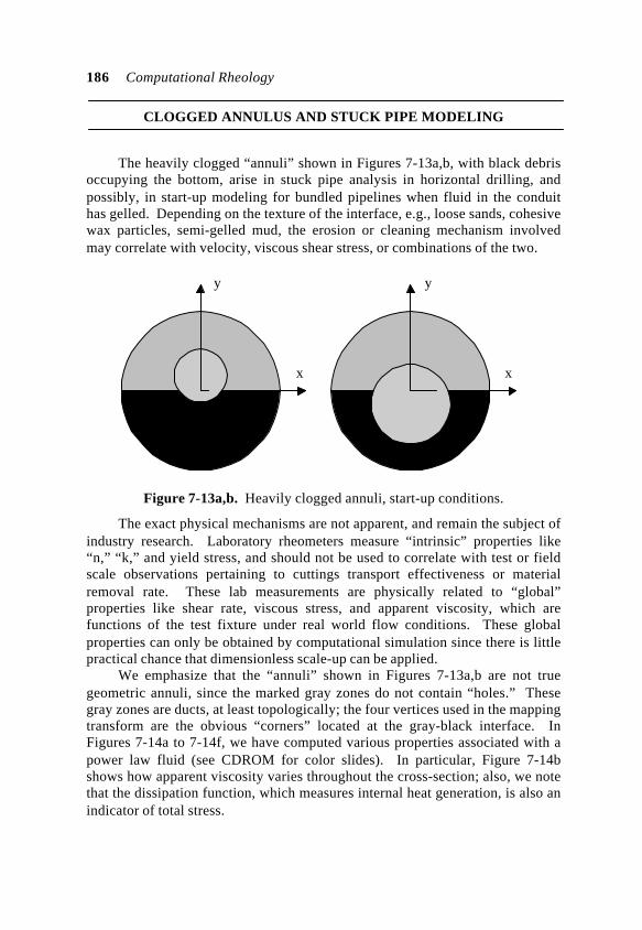
186 Computational Rheology
CLOGGED ANNULUS AND STUCK PIPE MODELING
The heavily clogged “annuli” shown in Figures 7-13a,b, with black debrisoccupying the bottom, arise in stuck pipe analysis in horizontal drilling, andpossibly, in start-up modeling for bundled pipelines when fluid in the conduithas gelled. Depending on the texture of the interface, e.g., loose sands, cohesivewax particles, semi-gelled mud, the erosion or cleaning mechanism involvedmay correlate with velocity, viscous shear stress, or combinations of the two.
x
y y
x
Figure 7-13a,b. Heavily clogged annuli, start-up conditions.
The exact physical mechanisms are not apparent, and remain the subject ofindustry research. Laboratory rheometers measure “intrinsic” properties like“n,” “k,” and yield stress, and should not be used to correlate with test or fieldscale observations pertaining to cuttings transport effectiveness or materialremoval rate. These lab measurements are physically related to “global”properties like shear rate, viscous stress, and apparent viscosity, which arefunctions of the test fixture under real world flow conditions. These globalproperties can only be obtained by computational simulation since there is littlepractical chance that dimensionless scale-up can be applied.
We emphasize that the “annuli” shown in Figures 7-13a,b are not truegeometric annuli, since the marked gray zones do not contain “holes.” Thesegray zones are ducts, at least topologically; the four vertices used in the mappingtransform are the obvious “corners” located at the gray-black interface. InFigures 7-14a to 7-14f, we have computed various properties associated with apower law fluid (see CDROM for color slides). In particular, Figure 7-14bshows how apparent viscosity varies throughout the cross-section; also, we notethat the dissipation function, which measures internal heat generation, is also anindicator of total stress.
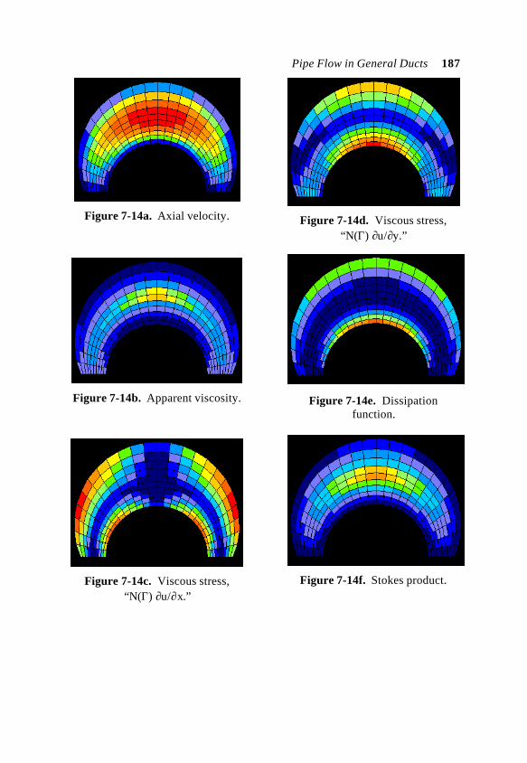
Pipe Flow in General Ducts 187
Figure 7-14a. Axial velocity.
Figure 7-14b. Apparent viscosity.
Figure 7-14c. Viscous stress,“N(Γ) ∂u/∂x.”
Figure 7-14d. Viscous stress,“N(Γ) ∂u/∂y.”
Figure 7-14e. Dissipationfunction.
Figure 7-14f. Stokes product.
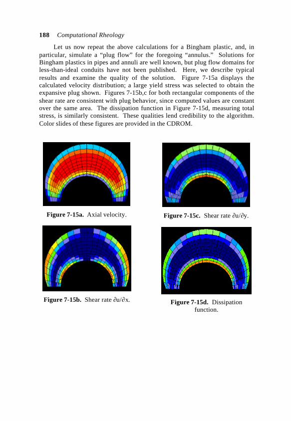
188 Computational Rheology
Let us now repeat the above calculations for a Bingham plastic, and, inparticular, simulate a “plug flow” for the foregoing “annulus.” Solutions forBingham plastics in pipes and annuli are well known, but plug flow domains forless-than-ideal conduits have not been published. Here, we describe typicalresults and examine the quality of the solution. Figure 7-15a displays thecalculated velocity distribution; a large yield stress was selected to obtain theexpansive plug shown. Figures 7-15b,c for both rectangular components of theshear rate are consistent with plug behavior, since computed values are constantover the same area. The dissipation function in Figure 7-15d, measuring totalstress, is similarly consistent. These qualities lend credibility to the algorithm.Color slides of these figures are provided in the CDROM.
Figure 7-15a. Axial velocity.
Figure 7-15b. Shear rate ∂u/∂x.
Figure 7-15c. Shear rate ∂u/∂y.
Figure 7-15d. Dissipationfunction.
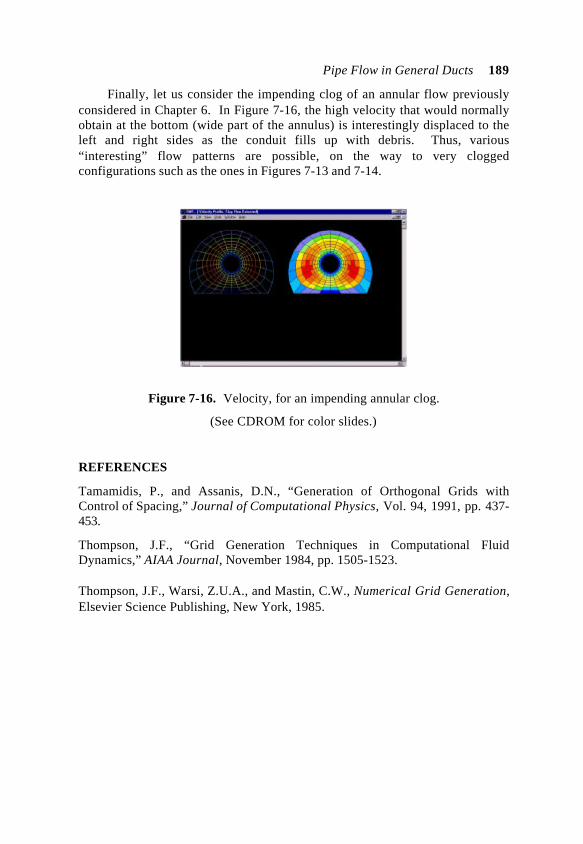
Pipe Flow in General Ducts 189
Finally, let us consider the impending clog of an annular flow previouslyconsidered in Chapter 6. In Figure 7-16, the high velocity that would normallyobtain at the bottom (wide part of the annulus) is interestingly displaced to theleft and right sides as the conduit fills up with debris. Thus, various“interesting” flow patterns are possible, on the way to very cloggedconfigurations such as the ones in Figures 7-13 and 7-14.
Figure 7-16. Velocity, for an impending annular clog.
(See CDROM for color slides.)
REFERENCES
Tamamidis, P., and Assanis, D.N., “Generation of Orthogonal Grids withControl of Spacing,” Journal of Computational Physics, Vol. 94, 1991, pp. 437-453.
Thompson, J.F., “Grid Generation Techniques in Computational FluidDynamics,” AIAA Journal, November 1984, pp. 1505-1523.
Thompson, J.F., Warsi, Z.U.A., and Mastin, C.W., Numerical Grid Generation,Elsevier Science Publishing, New York, 1985.
190
8
Solids Deposition Modeling
What is “solids deposition modeling” and what is its role in pipe or annularflow dynamics? Although numerous studies have been directed, for instance, atwax deposition and hydrate formation, none have addressed the dynamicinteraction between the solids deposition process and the velocity field impartedby the flowing non-Newtonian fluid. The latter serves dual functions: it assistswith solid particle placement, but at the same time, the viscous stress fieldassociated with it tends to remove particles that have adhered to solid surfaces.
Until now, determining the velocity field alone has proven difficult, if notimpossible: nonlinear flow equations must be solved for geometric domains thatare far from ideal in shape. However, the methods developed in Chapter 2 forannular flow and Chapter 7 for general duct flow permit fast and robustsolutions, and also, efficient post-processing and visual display for quantitieslike apparent viscosity, shear rate, and viscous stress. In this sense, “half” of theproblem has been resolved, and in this chapter, we address the remaining half.
In order to understand the overall philosophy, it is useful to return to theproblem of mudcake formation and erosion, and of cuttings transport, firstconsidered in Chapter 5. As we have noted, the plugging or cleaning of aborehole annulus can be a dynamic, time-dependent process. For example, theinability of the low side flow to remove cuttings results in debris bed formation,when cuttings combine with mudcake to form mechanical structures. Forcedfiltration of drilling mud into the formation compacts these beds, and individualparticle identities are lost: the resulting beds, characterized by well-defined yieldstresses, alter the shape of the borehole annulus and the properties of the flow.
But the bed can be eroded or removed, provided the viscous stressimparted by the flowing mud in the modified annulus exceeds the yield value. Ifthis is not possible, plugging will result and stuck pipe is possible. On the otherhand, alternative remedial actions are possible. The driller can change thecomposition of the mud to promote more effective cleaning, increase thevolumetric flow rate, or both. Successfully doing so erodes cuttingsaccumulations, and ideally, promotes dynamic “self-cleaning” of the hole.

Solids Deposition Modeling 191
In a sense, developing a new “constitutive relation,” e.g., postulatingNewtonian or power law properties, and deriving complementary flow equationsis simpler than designing solids deposition models. The mathematical processneeded to “place” stress-strain relations in momentum differential equation formis more straightforward than the cognitive process required to understand everystep of a new physical phenomenon, e.g., wax deposition or hydrate formation.In this chapter, we introduce a philosophy behind modeling solids deposition,and as a first step, develop a simple model for mudcake and cuttings bed buildupover porous rock. We emphasize that there are no simple answers: eachproblem is unique, and the developmental process is very iterative.
Mudcake buildup on porous rock. Borehole annuli are lined with slowlythickening mudcake that, over large time scales, will reduce cross-sectional size.However, dynamic equilibrium is usually achieved because erosive forces in theflow stream limit such thickening. As a first step in understanding this process,growth in the absence of erosion must be characterized, but even this requires adetailed picture of the physics. The reader should carefully consider the stepsneeded in designing deposition models, taking this example as a model.
Since the permeability of the formation greatly exceeds that of mudcake,and the thickness of mudcake is small compared with the borehole radius, wecan model cake growth in the idealized lineal flow test setup in Figure 8-1. Weconsider a one-dimensional experiment where mud, in essence a suspension ofclay particles in water, is allowed to flow through filter paper. Initially, the flowrate is rapid. But as time progresses, solid particles (typically 6%-40% byvolume for light to heavy muds) such as barite are deposited onto the surface ofthe paper, forming a mudcake that, in turn, retards the passage of mud filtrate byvirtue of the resistance to flow that the cake provides.
Mud
MudcakeFilter paper
Filtrate
Flow direction
Figure 8-1. Simple laboratory mudcake buildup experiment.
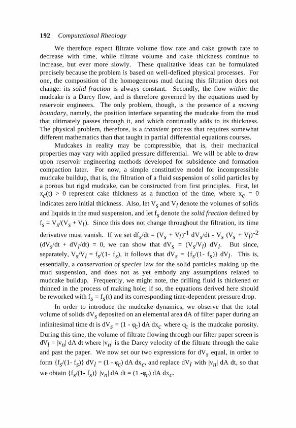
192 Computational Rheology
We therefore expect filtrate volume flow rate and cake growth rate todecrease with time, while filtrate volume and cake thickness continue toincrease, but ever more slowly. These qualitative ideas can be formulatedprecisely because the problem is based on well-defined physical processes. Forone, the composition of the homogeneous mud during this filtration does notchange: its solid fraction is always constant. Secondly, the flow within themudcake is a Darcy flow, and is therefore governed by the equations used byreservoir engineers. The only problem, though, is the presence of a movingboundary, namely, the position interface separating the mudcake from the mudthat ultimately passes through it, and which continually adds to its thickness.The physical problem, therefore, is a transient process that requires somewhatdifferent mathematics than that taught in partial differential equations courses.
Mudcakes in reality may be compressible, that is, their mechanicalproperties may vary with applied pressure differential. We will be able to drawupon reservoir engineering methods developed for subsidence and formationcompaction later. For now, a simple constitutive model for incompressiblemudcake buildup, that is, the filtration of a fluid suspension of solid particles bya porous but rigid mudcake, can be constructed from first principles. First, letxc(t) > 0 represent cake thickness as a function of the time, where xc = 0
indicates zero initial thickness. Also, let Vs and Vl denote the volumes of solids
and liquids in the mud suspension, and let fs denote the solid fraction defined by
fs = Vs/(Vs + Vl ). Since this does not change throughout the filtration, its time
derivative must vanish. If we set dfs/dt = (Vs + Vl )-1 dVs/dt - Vs (Vs + Vl)-2
(dVs/dt + dVl/dt) = 0, we can show that dVs = (Vs/Vl) dVl. But since,
separately, Vs/Vl = fs/(1- fs), it follows that dVs = fs/(1- fs) dVl . This is,
essentially, a conservation of species law for the solid particles making up themud suspension, and does not as yet embody any assumptions related tomudcake buildup. Frequently, we might note, the drilling fluid is thickened orthinned in the process of making hole; if so, the equations derived here shouldbe reworked with fs = fs(t) and its corresponding time-dependent pressure drop.
In order to introduce the mudcake dynamics, we observe that the totalvolume of solids dVs deposited on an elemental area dA of filter paper during an
infinitesimal time dt is dVs = (1 - φc) dA dxc where φc is the mudcake porosity.
During this time, the volume of filtrate flowing through our filter paper screen isdVl = |vn| dA dt where |vn| is the Darcy velocity of the filtrate through the cake
and past the paper. We now set our two expressions for dVs equal, in order to
form fs/(1- fs) dVl = (1 - φc) dA dxc, and replace dVl with |vn| dA dt, so that
we obtain fs/(1- fs) |vn| dA dt = (1 -φc) dA dxc.
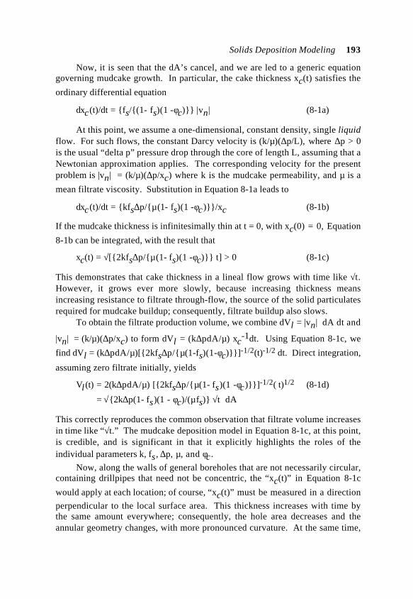
Solids Deposition Modeling 193
Now, it is seen that the dA’s cancel, and we are led to a generic equationgoverning mudcake growth. In particular, the cake thickness xc(t) satisfies the
ordinary differential equation
dxc(t)/dt = fs/(1- fs)(1 -φc) |vn| (8-1a)
At this point, we assume a one-dimensional, constant density, single liquidflow. For such flows, the constant Darcy velocity is (k/µ)(∆p/L), where ∆p > 0is the usual “delta p” pressure drop through the core of length L, assuming that aNewtonian approximation applies. The corresponding velocity for the presentproblem is |vn| = (k/µ)(∆p/xc) where k is the mudcake permeability, and µ is a
mean filtrate viscosity. Substitution in Equation 8-1a leads to
dxc(t)/dt = kfs∆p/µ(1- fs)(1 -φc)/xc (8-1b)
If the mudcake thickness is infinitesimally thin at t = 0, with xc(0) = 0, Equation
8-1b can be integrated, with the result that
xc(t) = √[2kfs∆p/µ(1- fs)(1 -φc) t] > 0 (8-1c)
This demonstrates that cake thickness in a lineal flow grows with time like √t.However, it grows ever more slowly, because increasing thickness meansincreasing resistance to filtrate through-flow, the source of the solid particulatesrequired for mudcake buildup; consequently, filtrate buildup also slows.
To obtain the filtrate production volume, we combine dVl = |vn| dA dt and
|vn| = (k/µ)(∆p/xc) to form dVl = (k∆pdA/µ) xc-1dt. Using Equation 8-1c, we
find dVl = (k∆pdA/µ)[2kfs∆p/µ(1-fs)(1-φc)]-1/2(t)-1/2 dt. Direct integration,
assuming zero filtrate initially, yields
Vl (t) = 2(k∆pdA/µ) [2kfs∆p/µ(1- fs)(1 -φc)]-1/2( t)1/2 (8-1d)
= √2k∆p(1- fs)(1 - φc)/(µfs) √t dA
This correctly reproduces the common observation that filtrate volume increasesin time like “√t.” The mudcake deposition model in Equation 8-1c, at this point,is credible, and is significant in that it explicitly highlights the roles of theindividual parameters k, fs, ∆p, µ, and φc .
Now, along the walls of general boreholes that are not necessarily circular,containing drillpipes that need not be concentric, the “xc(t)” in Equation 8-1c
would apply at each location; of course, “xc(t)” must be measured in a direction
perpendicular to the local surface area. This thickness increases with time bythe same amount everywhere; consequently, the hole area decreases and theannular geometry changes, with more pronounced curvature. At the same time,
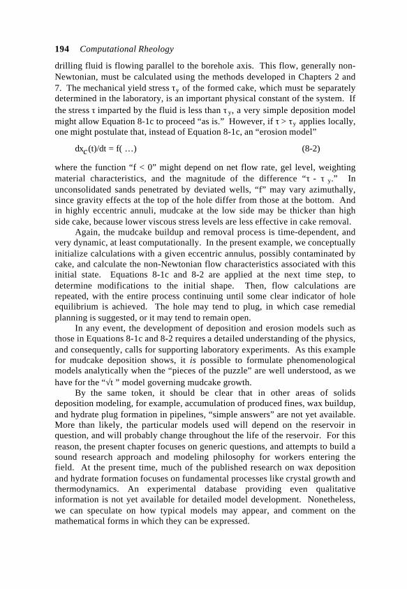
194 Computational Rheology
drilling fluid is flowing parallel to the borehole axis. This flow, generally non-Newtonian, must be calculated using the methods developed in Chapters 2 and7. The mechanical yield stress τ y of the formed cake, which must be separatelydetermined in the laboratory, is an important physical constant of the system. Ifthe stress τ imparted by the fluid is less than τ y, a very simple deposition modelmight allow Equation 8-1c to proceed “as is.” However, if τ > τ y applies locally,one might postulate that, instead of Equation 8-1c, an “erosion model”
dxc(t)/dt = f( …) (8-2)
where the function “f < 0” might depend on net flow rate, gel level, weightingmaterial characteristics, and the magnitude of the difference “τ - τ y.” Inunconsolidated sands penetrated by deviated wells, “f” may vary azimuthally,since gravity effects at the top of the hole differ from those at the bottom. Andin highly eccentric annuli, mudcake at the low side may be thicker than highside cake, because lower viscous stress levels are less effective in cake removal.
Again, the mudcake buildup and removal process is time-dependent, andvery dynamic, at least computationally. In the present example, we conceptuallyinitialize calculations with a given eccentric annulus, possibly contaminated bycake, and calculate the non-Newtonian flow characteristics associated with thisinitial state. Equations 8-1c and 8-2 are applied at the next time step, todetermine modifications to the initial shape. Then, flow calculations arerepeated, with the entire process continuing until some clear indicator of holeequilibrium is achieved. The hole may tend to plug, in which case remedialplanning is suggested, or it may tend to remain open.
In any event, the development of deposition and erosion models such asthose in Equations 8-1c and 8-2 requires a detailed understanding of the physics,and consequently, calls for supporting laboratory experiments. As this examplefor mudcake deposition shows, it is possible to formulate phenomenologicalmodels analytically when the “pieces of the puzzle” are well understood, as wehave for the “√t ” model governing mudcake growth.
By the same token, it should be clear that in other areas of solidsdeposition modeling, for example, accumulation of produced fines, wax buildup,and hydrate plug formation in pipelines, “simple answers” are not yet available.More than likely, the particular models used will depend on the reservoir inquestion, and will probably change throughout the life of the reservoir. For thisreason, the present chapter focuses on generic questions, and attempts to build asound research approach and modeling philosophy for workers entering thefield. At the present time, much of the published research on wax depositionand hydrate formation focuses on fundamental processes like crystal growth andthermodynamics. An experimental database providing even qualitativeinformation is not yet available for detailed model development. Nonetheless,we can speculate on how typical models may appear, and comment on themathematical forms in which they can be expressed.
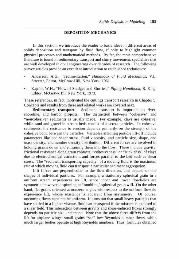
Solids Deposition Modeling 195
DEPOSITION MECHANICS
In this section, we introduce the reader to basic ideas in different areas ofsolids deposition and transport by fluid flow, if only to highlight commonphysical processes and mathematical methods. By far, the most comprehensiveliterature is found in sedimentary transport and slurry movement, specialties thatare well developed in civil engineering over decades of research. The followingsurvey articles provide an excellent introduction to established techniques:
• Anderson, A.G., “Sedimentation,” Handbook of Fluid Mechanics, V.L.Streeter, Editor, McGraw-Hill, New York, 1961.
• Kapfer, W.H., “Flow of Sludges and Slurries,” Piping Handbook, R. King,Editor, McGraw-Hill, New York, 1973.
These references, in fact, motivated the cuttings transport research in Chapter 5.Concepts and results from these and related works are covered next.
Sedimentary transport. Sediment transport is important to river,shoreline, and harbor projects. The distinction between “cohesive” and“noncohesive” sediments is usually made. For example, clays are cohesive,while sand and gravel in stream beds consist of discrete particles. In cohesivesediments, the resistance to erosion depends primarily on the strength of thecohesive bond between the particles. Variables affecting particle lift-off includeparameters like bed shear stress, fluid viscosity, and particle size, shape, andmass density, and number density distribution. Different forces are involved inholding grains down and entraining them into the flow. These include gravity,frictional resistance along grain contacts, “cohesiveness” or “stickiness” of claysdue to electrochemical attraction, and forces parallel to the bed such as shearstress. The “sediment transporting capacity” of a moving fluid is the maximumrate at which moving fluid can transport a particular sediment aggregation.
Lift forces are perpendicular to the flow direction, and depend on theshapes of individual particles. For example, a stationary spherical grain in auniform stream experiences no lift, since upper and lower flowfields aresymmetric; however, a spinning or “tumbling” spherical grain will. On the otherhand, flat grains oriented at nonzero angles with respect to the uniform flow doexperience lift, whose existence is apparent from asymmetry. Of course,oncoming flows need not be uniform. It turns out that small heavy particles thathave settled in a lighter viscous fluid can resuspend if the mixture is exposed toa shear field. This interaction between gravity and shear-induced fluxes stronglydepends on particle size and shape. Note that the above force differs from thelift for airplane wings: small grains “see” low Reynolds number flows, whilemuch larger bodies operate at high Reynolds numbers. Thus, formulas obtained
196 Computational Rheology
in different fluid specialties must be carefully evaluated before they are used indeposition modeling. In either case, mathematical analysis is very difficult.
Once lifted into the flow stream, overall movement is dictated by thevertical “settling velocity” of the particle, and the velocity in the main flow.Settling velocity is determined by balancing buoyancy and laminar drag forces,with the latter strongly dependent on fluid rheology. For Newtonian flows, theclassic Stokes solution applies; for non-Newtonian flows, analytical solutionsare not available. Different motions are possible. Finer silts and clays will moreor less float within a moving fluid. On the other hand, sand and gravel are likelyto travel close to bed; those that “roll and drag” along the bottom move bytraction, while those that “hop, skip, and jump” move by the process of saltation.
In general, modeling non-Newtonian flow past single stationary particlesrepresents a difficult endeavor, even for the most accomplished mathematicians.Flows past unconstrained bodies are even more challenging. Finally, modelingflows past aggregates of particles is likely to be impossible, without additionalsimplifying statistical assumptions. For these reasons, useful and practicaldeposition and transport models are likely to be empirical, so that scalablelaboratory experiments are highly encouraged. Simpler “ideal” flow setups thatshed physical insight on key parameters are likely to be more useful than“practical, engineering” examples that include too many interacting variables.
Slurry transport. A large body of literature exists for slurry transport,e.g., coal slurries, slurries in mining applications, slurries in process plants, andso on. A comprehensive review is neither possible nor necessary, since water isthe carrier fluid in the majority of references. But many fundamental ideas andapproaches apply. Early references provide discussions on sewage sludgeremoval, emphasizing prevalent non-Newtonian behavior, while acknowledgingthat computations are not practical. They also discuss settling phenomena inslurries, e.g., the influence of particle size, particle density, and fluid viscosity.
“Minimum velocity” formulas are available that, under the assumptionscited, are useful in ensuring clean ducts when the carrier fluid is water. Thenotion of “critical tractive force,” i.e., the value of shear stress at which bedmovement initiates, is introduced; this concept was important in our discussionsof cutting transport. Both “velocity” and “stress” criteria are used later in thischapter to construct illustrative numerical models of eroding flows. Also, thedistinction between transport in closed conduits and open channels is made.
The literature additionally addresses the effects of channel obstructions andthe formation of sediment waves; again, restrictions to water as the carrier fluid,are required. Numerous empirical formulas for Q that would give cleanconduits are available in the literature; however, their applicability to oilfielddebris, waxes, and hydrates is uncertain. While we carefully distinguishbetween velocity and stress as distinctly different erosion mechanisms, we notethat, in some flow, the distinction is less clear. At times, for example, thedecrease in bed shear stress is primarily a function of decreasing flow velocity.
Solids Deposition Modeling 197
WAXES AND PARAFFINS, BASIC IDEAS
As hot crude flows from reservoirs into cold pipelines, with lowtemperatures typical under deep subsea conditions, wax crystals may form alongsolid surfaces when wall temperatures drop below the “cloud point” or “waxappearance temperature.” Crystals may grow in size until the wall is fullycovered, with the possibility of encapsulating oil in the wax layers. Waxdeposition can grow preferentially on one side of the pipe due to gravitysegregation. As wax thickness builds, the pressure drop along the pipe must beincreased to maintain constant flow rate, and power requirements increase.Constant pressure processes would yield decreasing flow rates.
Paraffin deposition can be controlled through various means. Insulationand direct heating pipe will reduce exposure to the cold environment.Mechanical pigging is possible. Chemical inhibitors are also used. For example,surfactants or dispersants alter the ability of wax particles to adhere to eachother or to pipe wall surfaces; in the language of sedimentary transport, theybecome less cohesive, and behave more like discrete entities. Biochemicalmethods, for instance, use of bacteria to control wax growth.
In this book, we will address the effect of nonlinear fluid rheology andnoncircular duct flow in facilitating wax erosion. The “critical tractive force”ideas developed in slurry transport, extended in Chapter 5 to cuttings removal,again apply to bed-like deposits. Recent authors, for example, introduce“critical wax tension” analogously, defined as the critical shear force required toremove a unit thickness of wax deposit; the exact magnitude depends on oilcomposition, wax content, temperature, buildup history, and aging.
More complications. Paraffin deposition involves thermodynamics, butother operational consequences arise that draw from all physical disciplines.• Electrokinetic effects may be important with heavy organic constituents.
Potential differences along the conduit may develop due to the motion ofcharged particles; these induce alterations in colloidal particle chargesdownstream which promote deposition. That is, electrical charges in thecrude may encourage migration of separated waxes to the pipe wall.
• In low flow rate pipelines, certain waxes sink because of gravity, and formsludge layers at the low side. Also, density segregation can also lead torecirculating flows of the type modeled in Chapter 4.
• For lighter waxes, buoyancy can cause precipitated wax to collect at the topof the pipe (in the simulations performed in this chapter, no distinction ismade between “top” and “bottom,” since our “snapshots” can be turned“upside-down”).
198 Computational Rheology
• Deposited wax will increase wall roughness and therefore increase friction,thus reducing pipeline flow capacity.
• Suspended particulates such as asphaltenes, formation fines, corrosionproducts, silt, and sand, for instance, may encourage wax precipitation,acting as nuclei for wax separation and accumulation. Wax particles soseparated may not necessarily deposit along walls; they may remain insuspension, altering the rheology of the carrier fluid, affecting its ability to“throw” particles against pipe walls or to remove wax deposits by erosion.
• Although significant deposition is unlikely under isothermal conditions, thatis, when pipeline crude and ocean temperatures are in equilibrium, walldeposits may nonetheless form. Pipe roughness, for instance, can initiatestacking, leading to local accumulations that may further grow.
Wax precipitation in detail. Waxy crude may contain a variety of lightand intermediate hydrocarbons, e.g., paraffins, aromatics, naphtenic, wax, heavyorganic compounds, and low amount of resins, asphaltenes, organo-metallics.Wax in crudes consists of paraffin (C18-C36) and naphtenic (C30-C60)hydrocarbons. These wax components exist in various states, that is, gas, liquid,or solid, depending on temperature and pressure. When wax freezes, crystals areformed. Those formed from paraffin wax are known as “macrocrystalline wax,”while those originating from naphtenes are “microcrystalline.”
When the temperature of a waxy crude is decreased, the heavier fractionsin wax content appear first. The “cloud point” or “wax appearance temperature”is the temperature below which the oil is saturated with wax. Deposition occurswhen the temperature of the crude falls below cloud point. Paraffin willprecipitate under slight changes in equilibrium conditions, causing loss ofsolubility of the wax in the crude. Wax nucleation and growth may occur alongthe pipe surface and within the bulk fluid. Precipitation within the fluid causesits viscosity to increase and alters the non-Newtonian characteristics of thecarrier fluid. Increases in frictional drag may initiate pumping problems andhigher overall pipe pressures. Note that the carrier fluid is rarely a single-phaseflow. More often than not, wax deposition occurs in three-phase oil, water, andgas flow, over a range of gas-oil ratios, water cuts, and flow patterns, which canvary significantly with pipe inclination angle.
Wax deposition control. The most direct means of control, though notnecessarily the least inexpensive, target wall temperature by insulation orheating, possibly through internally heated pipes as discussed in Chapter 6. Butthe environment is far from certain. Some deposits do not disappear on heatingand are not fully removed by pigging. Crudes may contain heavy organics likeasphaltene and resin, which may not crystallize upon cooling and may not havedefinite freezing points; these interact with wax differently, and may preventwax crystal formation or enhance it. Solvents provide a different alternative.However, those containing benzene, ethyl benzene, toluene, and so on, are
Solids Deposition Modeling 199
encountering opposition from regulatory and environmental concerns. Theproblems are acute for offshore applications; inexpensive and environmentallyfriendly control approaches with minimal operational impact are desired.
Wax growth on solid surfaces, under static conditions, is believed to occurby molecular diffusion. Behind most deposition descriptions are liquid phasemodels and equations of state, with the exact composition of the wax phasedetermined by the model and the physical properties of the petroleum fractions.We do not attempt to understand the detailed processes behind wax precipitationand deposition in this book. Instead, we focus on fluid-dynamical modelingissues, demonstrating how non-Newtonian flows can be calculated for difficult“real world” duct geometries that are less than ideal. The “mere” determinationof the flowfield itself is significant, since it provides information to evaluatedifferent modes of deposition and to address important remediation issues.
For example, as in sedimentary transport, flow nonuniformities play dualroles: they may “throw” particles onto surfaces, where they adhere, or they canremove buildups by viscous shear. Both effects must be studied, in light ofexperimental data, using the background velocity and stress fields our analysisprovides. The modeling approaches reported in this book hope to establish thehydrodynamic backbone that makes accurate modeling of these phenomenapossible. For example, is it possible to design a fluid that keeps particlessuspended, or perhaps, to understand the conditions under which the flow is self-cleaning? What are rheological effects of chemical solvents? Wax can causecrude oil to gel and deposit on tubular surfaces. What shear stresses are requiredto remove them? And finally, waxy crude oil may gel after a period ofshutdown. What levels of pressure are required to initiate start-up of flow?
Modeling dynamic wax deposition. In principle, modeling the dynamic,time-dependent interaction between waxy deposits attempting to grow, and ductflows attempting to erode them, is similar to, although slightly morecomplicated than, the mudcake model developed earlier. The deposition, orgrowth model, shown conceptually in Figure 8-2a, consists of two parts, namely,a thermal component in which buildup is driven by temperature gradients, and amechanical component in which velocity “throws” additional particles that haveprecipitated in the bulk fluid into the wax-lined pipe surface. This velocity maybe coupled to the temperature environment, as discussed in Chapter 6. Varioussolids convection models are available in the fluids literature, and, in general,different deposition models are needed in different production scenarios.
The competing erosive model is schematically shown in Figure 8-2b, inwhich we emphasize the role of non-Newtonian fluid stress at the walls; it issimilar to our model for cuttings transport removal from stiff beds. Wax yieldstress may be determined in the laboratory or inferred from mechanical piggingdata, e.g., see Souza Mendes et al. (1999) or related pipeline literature.
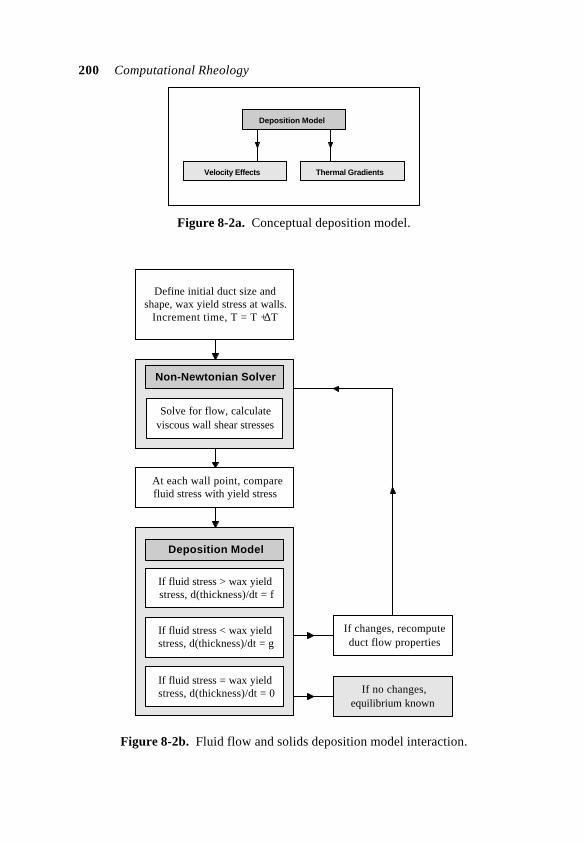
200 Computational Rheology
Deposition Model
Velocity Effects Thermal Gradients
Figure 8-2a. Conceptual deposition model.
At each wall point, comparefluid stress with yield stress
If no changes,equilibrium known
If fluid stress > wax yieldstress, d(thickness)/dt = f
If fluid stress < wax yieldstress, d(thickness)/dt = g
If fluid stress = wax yieldstress, d(thickness)/dt = 0
Deposition Model
If changes, recomputeduct flow properties
Define initial duct size andshape, wax yield stress at walls.
Increment time, T = T + ∆T
Non-Newtonian Solver
Solve for flow, calculateviscous wall shear stresses
Figure 8-2b. Fluid flow and solids deposition model interaction.
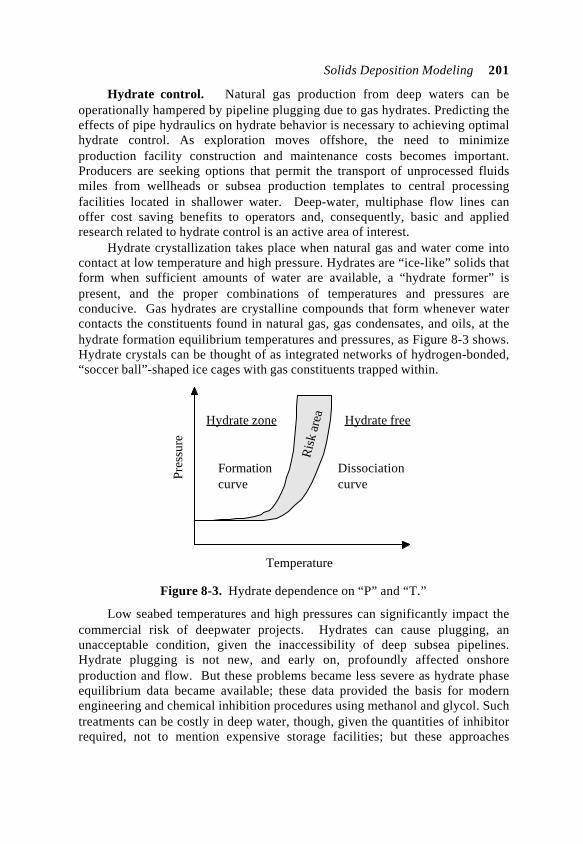
Solids Deposition Modeling 201
Hydrate control. Natural gas production from deep waters can beoperationally hampered by pipeline plugging due to gas hydrates. Predicting theeffects of pipe hydraulics on hydrate behavior is necessary to achieving optimalhydrate control. As exploration moves offshore, the need to minimizeproduction facility construction and maintenance costs becomes important.Producers are seeking options that permit the transport of unprocessed fluidsmiles from wellheads or subsea production templates to central processingfacilities located in shallower water. Deep-water, multiphase flow lines canoffer cost saving benefits to operators and, consequently, basic and appliedresearch related to hydrate control is an active area of interest.
Hydrate crystallization takes place when natural gas and water come intocontact at low temperature and high pressure. Hydrates are “ice-like” solids thatform when sufficient amounts of water are available, a “hydrate former” ispresent, and the proper combinations of temperatures and pressures areconducive. Gas hydrates are crystalline compounds that form whenever watercontacts the constituents found in natural gas, gas condensates, and oils, at thehydrate formation equilibrium temperatures and pressures, as Figure 8-3 shows.Hydrate crystals can be thought of as integrated networks of hydrogen-bonded,“soccer ball”-shaped ice cages with gas constituents trapped within.
Temperature
Pres
sure
Hydrate zone Hydrate free
Formationcurve
Dissociationcurve
Ris
k ar
ea
Figure 8-3. Hydrate dependence on “P” and “T.”
Low seabed temperatures and high pressures can significantly impact thecommercial risk of deepwater projects. Hydrates can cause plugging, anunacceptable condition, given the inaccessibility of deep subsea pipelines.Hydrate plugging is not new, and early on, profoundly affected onshoreproduction and flow. But these problems became less severe as hydrate phaseequilibrium data became available; these data provided the basis for modernengineering and chemical inhibition procedures using methanol and glycol. Suchtreatments can be costly in deep water, though, given the quantities of inhibitorrequired, not to mention expensive storage facilities; but these approaches
202 Computational Rheology
remain attractive, as recent research has led the way to more effective, lowtoxicity compounds as useful alternatives to methanol or glycol. Field andlaboratory studies have had some success, but problems remain that must besolved before the industry gains advantages in utilizing these inhibitors.
Operational considerations are also important to hydrate mitigation.Proper amounts of chemicals must arrive at target flowline locations at therequired time to control the rate of crystal formation, growth, agglomeration,and deposition. This combined chemical and hydrodynamic control strategy ingeneral multiphase pipeline environments must be effective over extended shut-in periods to accommodate a range of potential offshore operating scenarios.
Understanding the effects of chemicals on rheology and flow representsone aspect of the mitigation problem. In pipeline plugging, we are concerned, asnoted above, with the effects of obstructions on pressure drops and flow rates.On the other hand, natural hydrates represent a potentially important source ofnatural gas, although they can potentially clog pipelines. One possible deliverysolution is to convert associated gases into frozen hydrates, which are thenmixed with refrigerated crude oil, to form slurries, which are in turn pumpedthrough pipelines and into shuttle tankers for transport to shore. By blendingground hydrates with suitable carrier fluids, a transportable slurry can be formedthat efficiently delivers “gas” to market.
Several questions are immediately apparent. How finely should hydratesbe ground? What is the ideal “solids in fluid” concentration? Fineness, ofcourse, influences rheology; the solids that remain affect plugging, and thecombination controls delivery economics. And what happens as hydratesconvect into higher pressure pipeline regimes? In any event, we are concernedwith the pumpability of the slurry, and also, the ability of the slurry to erodehydrate plugs that have formed in the flow path. These considerations require amodel that is able to simulate flows in duct geometries that are far from circular.With it, we can simulate worst case conditions and optimize operations.
In this chapter, we will not focus on the physics and chemistry of hydrateformation, the kinetics of formation and agglomeration, or the physiochemicalcharacterization of the solid constituents. Instead, we will study flows past“hydrate plugs.” Wax buildup is “predictable” to the extent that depositions canbe found at top and low sides, and all too often, azimuthally about the entirecircumference. Hydrates, in contrast, may appear “randomly.” For example,they can form as layers separating gas on the top side and water on the low side.In terms of size, hydrate particles may vary from finely dispersed solid particlesto big lumps that stick to the walls of pipelines. Hydrate particle size isnonuniform and follows wide distribution densities. But, in general, large plugscan be found almost anywhere, a situation that challenges non-Newtonian flowmodeling in arbitrary ducts. Simulation is important in defining start-upprocedures, because large plugs are associated with extremely large pressuredrops that may be difficult to achieve in practice.
Solids Deposition Modeling 203
Pipe inclination may play a significant role for denser fluids. Ibraheem etal (1998) observe that, for their horizontal and 45o positions, predictions may beoptimistic since lift forces, virtual mass effects, and so on, are not incorporated,and that a two-dimensional model will be necessary. This caution is welljustified. In Chapter 4, we showed that density stratification can lead torecirculation vortices that plug the pipeline, while in Chapter 5, we showed that45o-70o inclinations are worst, even when density variations are ignored.
Recapitulation. Very subtle questions are possible. Can hydrate pipelineblockages lead to increased flowline pressures that facilitate additional hydrategrowth? Can viscous shear stresses developed within a carrier fluid, or perhapsa hydrate slurry, that support “self-cleaning,” which in turn eliminates isolatedplugs that form? Again, the formalism developed in Figure 8-2b for waxremoval applies, but now with Figure 8-2a replaced by one applicable to hydrateformation. We will show that numerical simulations can be convenientlyperformed for large, asymmetrically shaped plugs, that is, our grid generationand velocity solvers are truly “robust” in the numerical sense. Thus, it is clearthat the simulation methodology also applies to other types of conduits, valves,and fittings that can potentially support hydrate formation.
MODELING CONCEPTS AND INTEGRATION
Our mathematical description of time-dependent mudcake buildup, withouterosive effects, is relevant to wax buildup under nonisothermal conditions.Recall that once cake starts building, incremental growth of cake retards furtherbuildup, since additional resistance impedes fluid filtration. Thus, the rate ofcake growth should vary inversely with cake thickness; in fact, we had shown
dxc(t)/dt = kfs∆p/µ(1- fs)(1 -φc)/xc (8-1b)
Direct integration of “xc dxc = ..” leads “½ xc2 = ..t,” that is, the “ √t law,”
xc(t) = √ [2kfs∆p/µ(1- fs)(1 -φc) t] > 0 (8-1c)
In this section, we introduce some elementary, but preliminary ideas, with thehope of stimulating further research. These following illustrative examples weredesigned to be simple, to show how mathematics and physics go hand in hand.
Wax buildup due to temperature differences. Paraphrasing the above,“once wax starts building, incremental growth of wax retards further buildup,since additional insulation impedes heat transfer.” Let Rpipe denote the innerradius of the pipe, which is constant, and let R(t) < Rpipe denote the time-varyingradius of the wax-to-fluid interface. In cake buildup, growth rate is proportionalto the pressure gradient; here, it is proportional to the heat transfer rate, ortemperature gradient (T -Tpipe)/(R – Rpipe) by virtue of Fourier’s law ofconduction, with T being the fluid temperature. We therefore write, analogouslyto Equation 8-1b,
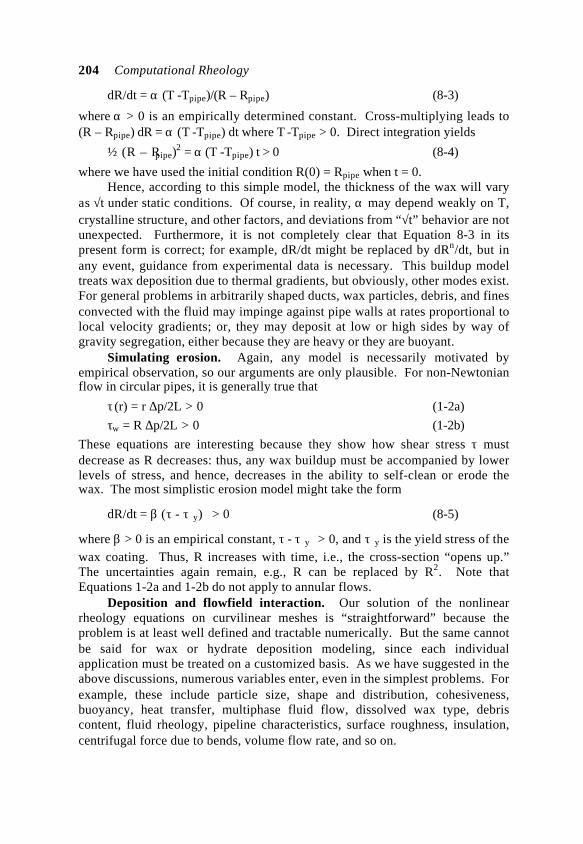
204 Computational Rheology
dR/dt = α (T -Tpipe)/(R – Rpipe) (8-3)
where α > 0 is an empirically determined constant. Cross-multiplying leads to(R – Rpipe) dR = α (T -Tpipe) dt where T -Tpipe > 0. Direct integration yields
½ (R – Rpipe)2 = α (T -Tpipe) t > 0 (8-4)
where we have used the initial condition R(0) = Rpipe when t = 0.Hence, according to this simple model, the thickness of the wax will vary
as √t under static conditions. Of course, in reality, α may depend weakly on T,crystalline structure, and other factors, and deviations from “√t” behavior are notunexpected. Furthermore, it is not completely clear that Equation 8-3 in itspresent form is correct; for example, dR/dt might be replaced by dRn/dt, but inany event, guidance from experimental data is necessary. This buildup modeltreats wax deposition due to thermal gradients, but obviously, other modes exist.For general problems in arbitrarily shaped ducts, wax particles, debris, and finesconvected with the fluid may impinge against pipe walls at rates proportional tolocal velocity gradients; or, they may deposit at low or high sides by way ofgravity segregation, either because they are heavy or they are buoyant.
Simulating erosion. Again, any model is necessarily motivated byempirical observation, so our arguments are only plausible. For non-Newtonianflow in circular pipes, it is generally true that
τ (r) = r ∆p/2L > 0 (1-2a)
τw = R ∆p/2L > 0 (1-2b)
These equations are interesting because they show how shear stress τ mustdecrease as R decreases: thus, any wax buildup must be accompanied by lowerlevels of stress, and hence, decreases in the ability to self-clean or erode thewax. The most simplistic erosion model might take the form
dR/dt = β (τ - τ y) > 0 (8-5)
where β > 0 is an empirical constant, τ - τ y > 0, and τ y is the yield stress of thewax coating. Thus, R increases with time, i.e., the cross-section “opens up.”The uncertainties again remain, e.g., R can be replaced by R2. Note thatEquations 1-2a and 1-2b do not apply to annular flows.
Deposition and flowfield interaction. Our solution of the nonlinearrheology equations on curvilinear meshes is “straightforward” because theproblem is at least well defined and tractable numerically. But the same cannotbe said for wax or hydrate deposition modeling, since each individualapplication must be treated on a customized basis. As we have suggested in theabove discussions, numerous variables enter, even in the simplest problems. Forexample, these include particle size, shape and distribution, cohesiveness,buoyancy, heat transfer, multiphase fluid flow, dissolved wax type, debriscontent, fluid rheology, pipeline characteristics, surface roughness, insulation,centrifugal force due to bends, volume flow rate, and so on.
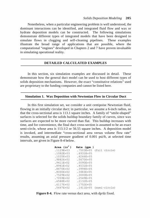
Solids Deposition Modeling 205
Nonetheless, when a particular engineering problem is well understood, thedominant interactions can be identified, and integrated fluid flow and wax orhydrate deposition models can be constructed. The following simulationsdemonstrate different types of integrated models that have been designed tosimulate flows in clogging and self-cleaning pipelines. These examplesillustrate the broad range of applications that are possible, where thecomputational “engines” developed in Chapters 2 and 7 have proven invaluablein simulating operational reality.
DETAILED CALCULATED EXAMPLES
In this section, six simulation examples are discussed in detail. Thesedemonstrate how the general duct model can be used to host different types ofsolids deposition mechanisms. However, the exact “constitutive relations” usedare proprietary to the funding companies and cannot be listed here.
Simulation 1. Wax Deposition with Newtonian Flow in Circular Duct
In this first simulation set, we consider a unit centipoise Newtonian fluid,flowing in an initially circular duct; in particular, we assume a 6-inch radius, sothat the cross-sectional area is 113.1 square inches. A family of “smile-shaped”surfaces is selected for the solids buildup boundary family of curves, since waxsurfaces are expected to be more curved than flat. This buildup increases withtime, and for convenience, the final duct cross-section is assumed to be an exactsemi-circle, whose area is 113.1/2 or 56.55 square inches. A deposition modelis invoked, and intermediate “cross-sectional area versus volume flow rate”results, assuming an axial pressure gradient of 0.001 psi/ft, at selected timeintervals, are given in Figure 8-4 below.
Area (in2 ) Rate (gpm ).1129E+03 .7503E+05 (full circle).1082E+03 .6931E+05.1035E+03 .6266E+05.9882E+02 .5670E+05.9411E+02 .5090E+05.8941E+02 .4531E+05.8470E+02 .3994E+05.8000E+02 .3483E+05.7529E+02 .3000E+05.7059E+02 .2549E+05.6588E+02 .2132E+05.6117E+02 .1752E+05.5647E+02 .1411E+05 (semi-circle)
Figure 8-4. Flow rate versus duct area, with dp/dz fixed.
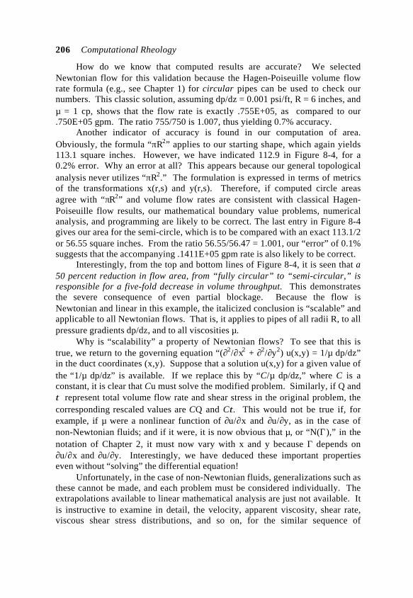
206 Computational Rheology
How do we know that computed results are accurate? We selectedNewtonian flow for this validation because the Hagen-Poiseuille volume flowrate formula (e.g., see Chapter 1) for circular pipes can be used to check ournumbers. This classic solution, assuming dp/dz = 0.001 psi/ft, R = 6 inches, andµ = 1 cp, shows that the flow rate is exactly .755E+05, as compared to our.750E+05 gpm. The ratio 755/750 is 1.007, thus yielding 0.7% accuracy.
Another indicator of accuracy is found in our computation of area.Obviously, the formula “πR2” applies to our starting shape, which again yields113.1 square inches. However, we have indicated 112.9 in Figure 8-4, for a0.2% error. Why an error at all? This appears because our general topologicalanalysis never utilizes “πR2.” The formulation is expressed in terms of metricsof the transformations x(r,s) and y(r,s). Therefore, if computed circle areasagree with “πR2” and volume flow rates are consistent with classical Hagen-Poiseuille flow results, our mathematical boundary value problems, numericalanalysis, and programming are likely to be correct. The last entry in Figure 8-4gives our area for the semi-circle, which is to be compared with an exact 113.1/2or 56.55 square inches. From the ratio 56.55/56.47 = 1.001, our “error” of 0.1%suggests that the accompanying .1411E+05 gpm rate is also likely to be correct.
Interestingly, from the top and bottom lines of Figure 8-4, it is seen that a50 percent reduction in flow area, from “fully circular” to “semi-circular,” isresponsible for a five-fold decrease in volume throughput. This demonstratesthe severe consequence of even partial blockage. Because the flow isNewtonian and linear in this example, the italicized conclusion is “scalable” andapplicable to all Newtonian flows. That is, it applies to pipes of all radii R, to allpressure gradients dp/dz, and to all viscosities µ.
Why is “scalability” a property of Newtonian flows? To see that this istrue, we return to the governing equation “(∂2/∂x2 + ∂2/∂y2) u(x,y) = 1/µ dp/dz”in the duct coordinates (x,y). Suppose that a solution u(x,y) for a given value ofthe “1/µ dp/dz” is available. If we replace this by “C/µ dp/dz,” where C is aconstant, it is clear that Cu must solve the modified problem. Similarly, if Q andτ represent total volume flow rate and shear stress in the original problem, thecorresponding rescaled values are CQ and Cτ. This would not be true if, forexample, if µ were a nonlinear function of ∂u/∂x and ∂u/∂y, as in the case ofnon-Newtonian fluids; and if it were, it is now obvious that µ, or “N(Γ),” in thenotation of Chapter 2, it must now vary with x and y because Γ depends on∂u/∂x and ∂u/∂y. Interestingly, we have deduced these important propertieseven without “solving” the differential equation!
Unfortunately, in the case of non-Newtonian fluids, generalizations such asthese cannot be made, and each problem must be considered individually. Theextrapolations available to linear mathematical analysis are just not available. Itis instructive to examine in detail, the velocity, apparent viscosity, shear rate,viscous shear stress distributions, and so on, for the similar sequence of
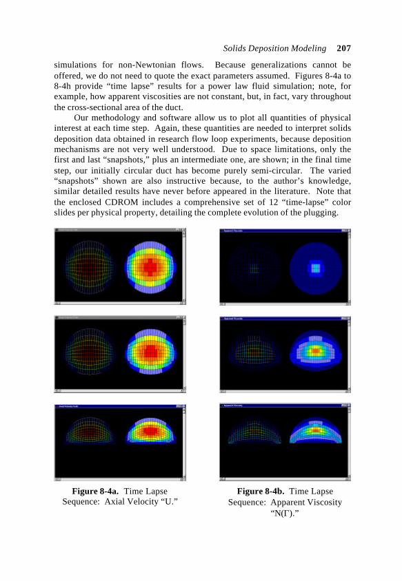
Solids Deposition Modeling 207
simulations for non-Newtonian flows. Because generalizations cannot beoffered, we do not need to quote the exact parameters assumed. Figures 8-4a to8-4h provide “time lapse” results for a power law fluid simulation; note, forexample, how apparent viscosities are not constant, but, in fact, vary throughoutthe cross-sectional area of the duct.
Our methodology and software allow us to plot all quantities of physicalinterest at each time step. Again, these quantities are needed to interpret solidsdeposition data obtained in research flow loop experiments, because depositionmechanisms are not very well understood. Due to space limitations, only thefirst and last “snapshots,” plus an intermediate one, are shown; in the final timestep, our initially circular duct has become purely semi-circular. The varied“snapshots” shown are also instructive because, to the author’s knowledge,similar detailed results have never before appeared in the literature. Note thatthe enclosed CDROM includes a comprehensive set of 12 “time-lapse” colorslides per physical property, detailing the complete evolution of the plugging.
Figure 8-4a. Time LapseSequence: Axial Velocity “U.”
Figure 8-4b. Time LapseSequence: Apparent Viscosity
“N(Γ).”
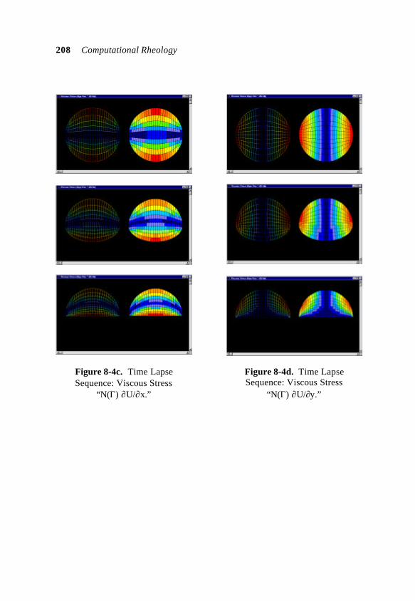
208 Computational Rheology
Figure 8-4c. Time LapseSequence: Viscous Stress
“N(Γ) ∂U/∂x.”
Figure 8-4d. Time LapseSequence: Viscous Stress
“N(Γ) ∂U/∂y.”
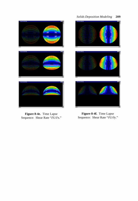
Solids Deposition Modeling 209
Figure 8-4e. Time LapseSequence: Shear Rate “∂U/∂x.”
Figure 8-4f. Time LapseSequence: Shear Rate “∂U/∂y.”
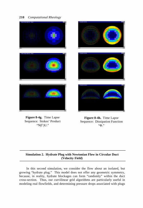
210 Computational Rheology
Figure 8-4g. Time LapseSequence: Stokes’ Product
“N(Γ)U.”
Figure 8-4h. Time LapseSequence: Dissipation Function
“Φ.”
Simulation 2. Hydrate Plug with Newtonian Flow in Circular Duct(Velocity Field)
In this second simulation, we consider the flow about an isolated, butgrowing “hydrate plug.” This model does not offer any geometric symmetry,because, in reality, hydrate blockages can form “randomly” within the ductcross-section. Thus, our curvilinear grid algorithms are particularly useful inmodeling real flowfields, and determining pressure drops associated with plugs
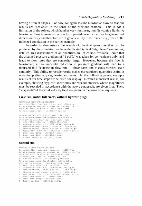
Solids Deposition Modeling 211
having different shapes. For now, we again assume Newtonian flow so that ourresults are “scalable” in the sense of the previous example. This is not alimitation of the solver, which handles very nonlinear, non-Newtonian fluids. ANewtonian flow is assumed here only to provide results that can be generalizeddimensionlessly and therefore are of greater utility to the reader, e.g., refer to theitalicized conclusion in the earlier example.
In order to demonstrate the wealth of physical quantities that can beproduced by the simulator, we have duplicated typical “high level” summaries;detailed area distributions of all quantities are, of course, available. Note thatthe assumed pressure gradient of “1 psi/ft” was taken for convenience only, andleads to flow rates that are somewhat large. However, because the flow isNewtonian, a thousand-fold reduction in pressure gradient will lead to athousand-fold decrease in flow rate. Shear rates and viscous stresses scalesimilarly. This ability to rescale results makes our tabulated quantities useful inobtaining preliminary engineering estimates. In the following pages, exampleresults of six time steps are selected for display. Detailed numerical results, forexample, showing “typical” shear rates and viscous stresses, whose magnitudesmust be rescaled in accordance with the above paragraph, are given first. Then,“snapshots” of the axial velocity field are given, in the same time sequence.
First run, initial full circle, without hydrate plug:
NEWTONIAN FLOW OPTION SELECTED.Newtonian flow, constant viscosity = 1.00000 cpAxial pressure gradient assumed as .1000E+01 psi/ft.Total volume flow rate = .7503E+08 gal/minCross-sectional area = .1129E+03 sq inch
TABULATION OF CALCULATED AVERAGE QUANTITIES:Area weighted means for absolute values takenover entire pipe (x,y) cross-sectional areaO Axial flow velocity = .2266E+07 in/secO Apparent viscosity = .1465E-06 lbf sec/sq inO Viscous stress, AppVis x dU/dx, = .1029E+00 psiO Viscous stress, AppVis x dU/dy, = .1230E+00 psiO Dissipation function = .2415E+06 lbf/(sec sq in)O Shear rate dU/dx = .7022E+06 1/secO Shear rate dU/dy = .8394E+06 1/secO Stokes product = .3321E+00 lbf/in
Second run:
NEWTONIAN FLOW OPTION SELECTED.Newtonian flow, constant viscosity = 1.00000 cpAxial pressure gradient assumed as .1000E+01 psi/ft.Total volume flow rate = .6925E+08 gal/minCross-sectional area = .1088E+03 sq inchTABULATION OF CALCULATED AVERAGE QUANTITIES:Area weighted means for absolute values takenover entire pipe (x,y) cross-sectional areaO Axial flow velocity = .2159E+07 in/secO Apparent viscosity = .1465E-06 lbf sec/sq inO Viscous stress, AppVis x dU/dx, = .1050E+00 psiO Viscous stress, AppVis x dU/dy, = .1176E+00 psiO Dissipation function = .2350E+06 lbf/(sec sq in)O Shear rate dU/dx = .7168E+06 1/secO Shear rate dU/dy = .8026E+06 1/secO Stokes product = .3163E+00 lbf/in
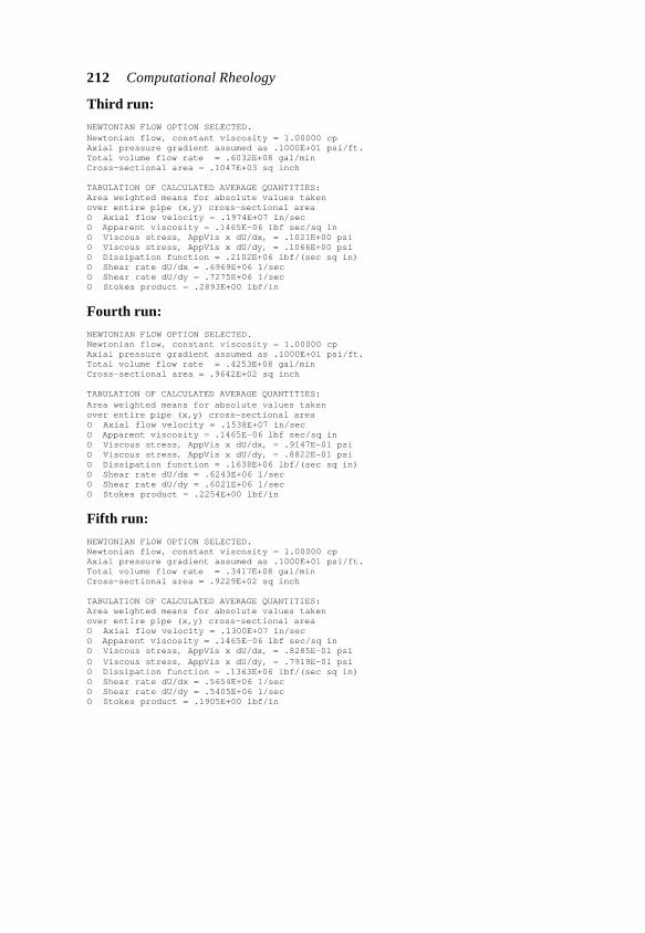
212 Computational Rheology
Third run:
NEWTONIAN FLOW OPTION SELECTED.Newtonian flow, constant viscosity = 1.00000 cpAxial pressure gradient assumed as .1000E+01 psi/ft.Total volume flow rate = .6032E+08 gal/minCross-sectional area = .1047E+03 sq inch
TABULATION OF CALCULATED AVERAGE QUANTITIES:Area weighted means for absolute values takenover entire pipe (x,y) cross-sectional areaO Axial flow velocity = .1974E+07 in/secO Apparent viscosity = .1465E-06 lbf sec/sq inO Viscous stress, AppVis x dU/dx, = .1021E+00 psiO Viscous stress, AppVis x dU/dy, = .1066E+00 psiO Dissipation function = .2102E+06 lbf/(sec sq in)O Shear rate dU/dx = .6969E+06 1/secO Shear rate dU/dy = .7275E+06 1/secO Stokes product = .2893E+00 lbf/in
Fourth run:
NEWTONIAN FLOW OPTION SELECTED.Newtonian flow, constant viscosity = 1.00000 cpAxial pressure gradient assumed as .1000E+01 psi/ft.Total volume flow rate = .4253E+08 gal/minCross-sectional area = .9642E+02 sq inch
TABULATION OF CALCULATED AVERAGE QUANTITIES:Area weighted means for absolute values takenover entire pipe (x,y) cross-sectional areaO Axial flow velocity = .1538E+07 in/secO Apparent viscosity = .1465E-06 lbf sec/sq inO Viscous stress, AppVis x dU/dx, = .9147E-01 psiO Viscous stress, AppVis x dU/dy, = .8822E-01 psiO Dissipation function = .1638E+06 lbf/(sec sq in)O Shear rate dU/dx = .6243E+06 1/secO Shear rate dU/dy = .6021E+06 1/secO Stokes product = .2254E+00 lbf/in
Fifth run:
NEWTONIAN FLOW OPTION SELECTED.Newtonian flow, constant viscosity = 1.00000 cpAxial pressure gradient assumed as .1000E+01 psi/ft.Total volume flow rate = .3417E+08 gal/minCross-sectional area = .9229E+02 sq inch
TABULATION OF CALCULATED AVERAGE QUANTITIES:Area weighted means for absolute values takenover entire pipe (x,y) cross-sectional areaO Axial flow velocity = .1300E+07 in/secO Apparent viscosity = .1465E-06 lbf sec/sq inO Viscous stress, AppVis x dU/dx, = .8285E-01 psiO Viscous stress, AppVis x dU/dy, = .7919E-01 psiO Dissipation function = .1363E+06 lbf/(sec sq in)O Shear rate dU/dx = .5654E+06 1/secO Shear rate dU/dy = .5405E+06 1/secO Stokes product = .1905E+00 lbf/in
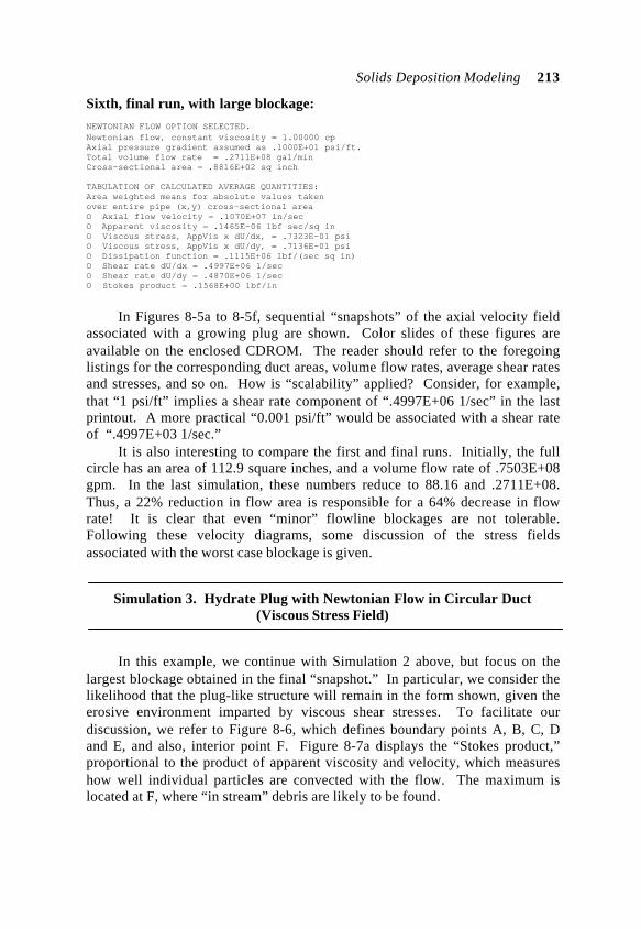
Solids Deposition Modeling 213
Sixth, final run, with large blockage:
NEWTONIAN FLOW OPTION SELECTED.Newtonian flow, constant viscosity = 1.00000 cpAxial pressure gradient assumed as .1000E+01 psi/ft.Total volume flow rate = .2711E+08 gal/minCross-sectional area = .8816E+02 sq inch
TABULATION OF CALCULATED AVERAGE QUANTITIES:Area weighted means for absolute values takenover entire pipe (x,y) cross-sectional areaO Axial flow velocity = .1070E+07 in/secO Apparent viscosity = .1465E-06 lbf sec/sq inO Viscous stress, AppVis x dU/dx, = .7323E-01 psiO Viscous stress, AppVis x dU/dy, = .7136E-01 psiO Dissipation function = .1115E+06 lbf/(sec sq in)O Shear rate dU/dx = .4997E+06 1/secO Shear rate dU/dy = .4870E+06 1/secO Stokes product = .1568E+00 lbf/in
In Figures 8-5a to 8-5f, sequential “snapshots” of the axial velocity fieldassociated with a growing plug are shown. Color slides of these figures areavailable on the enclosed CDROM. The reader should refer to the foregoinglistings for the corresponding duct areas, volume flow rates, average shear ratesand stresses, and so on. How is “scalability” applied? Consider, for example,that “1 psi/ft” implies a shear rate component of “.4997E+06 1/sec” in the lastprintout. A more practical “0.001 psi/ft” would be associated with a shear rateof “.4997E+03 1/sec.”
It is also interesting to compare the first and final runs. Initially, the fullcircle has an area of 112.9 square inches, and a volume flow rate of .7503E+08gpm. In the last simulation, these numbers reduce to 88.16 and .2711E+08.Thus, a 22% reduction in flow area is responsible for a 64% decrease in flowrate! It is clear that even “minor” flowline blockages are not tolerable.Following these velocity diagrams, some discussion of the stress fieldsassociated with the worst case blockage is given.
Simulation 3. Hydrate Plug with Newtonian Flow in Circular Duct(Viscous Stress Field)
In this example, we continue with Simulation 2 above, but focus on thelargest blockage obtained in the final “snapshot.” In particular, we consider thelikelihood that the plug-like structure will remain in the form shown, given theerosive environment imparted by viscous shear stresses. To facilitate ourdiscussion, we refer to Figure 8-6, which defines boundary points A, B, C, Dand E, and also, interior point F. Figure 8-7a displays the “Stokes product,”proportional to the product of apparent viscosity and velocity, which measureshow well individual particles are convected with the flow. The maximum islocated at F, where “in stream” debris are likely to be found.
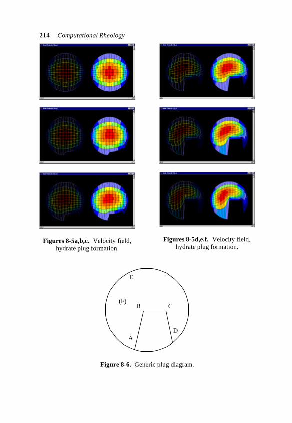
214 Computational Rheology
Figures 8-5a,b,c. Velocity field,hydrate plug formation.
Figures 8-5d,e,f. Velocity field,hydrate plug formation.
A
B C
D
E
(F)
Figure 8-6. Generic plug diagram.
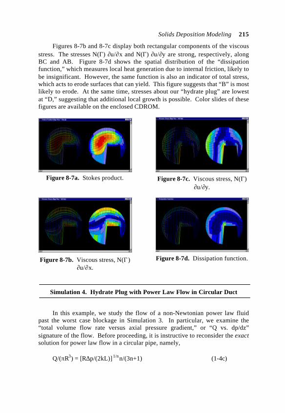
Solids Deposition Modeling 215
Figures 8-7b and 8-7c display both rectangular components of the viscousstress. The stresses N(Γ) ∂u/∂x and N(Γ) ∂u/∂y are strong, respectively, alongBC and AB. Figure 8-7d shows the spatial distribution of the “dissipationfunction,” which measures local heat generation due to internal friction, likely tobe insignificant. However, the same function is also an indicator of total stress,which acts to erode surfaces that can yield. This figure suggests that “B” is mostlikely to erode. At the same time, stresses about our “hydrate plug” are lowestat “D,” suggesting that additional local growth is possible. Color slides of thesefigures are available on the enclosed CDROM.
Figure 8-7a. Stokes product.
Figure 8-7b. Viscous stress, N(Γ)∂u/∂x.
Figure 8-7c. Viscous stress, N(Γ)∂u/∂y.
Figure 8-7d. Dissipation function.
Simulation 4. Hydrate Plug with Power Law Flow in Circular Duct
In this example, we study the flow of a non-Newtonian power law fluidpast the worst case blockage in Simulation 3. In particular, we examine the“total volume flow rate versus axial pressure gradient,” or “Q vs. dp/dz”signature of the flow. Before proceeding, it is instructive to reconsider the exactsolution for power law flow in a circular pipe, namely,
Q/(πR3) = [R∆p/(2kL)] 1/n
n/(3n+1) (1-4c)
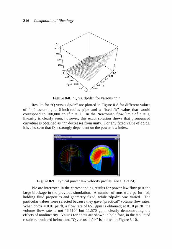
216 Computational Rheology
Figure 8-8. “Q vs. dp/dz” for various “n.”
Results for “Q versus dp/dz” are plotted in Figure 8-8 for different valuesof “n,” assuming a 6-inch-radius pipe and a fixed ‘k” value that wouldcorrespond to 100,000 cp if n = 1. In the Newtonian flow limit of n = 1,linearity is clearly seen, however, this exact solution shows that pronouncedcurvature is obtained as “n” decreases from unity. For any fixed value of dp/dz,it is also seen that Q is strongly dependent on the power law index.
Figure 8-9. Typical power law velocity profile (see CDROM).
We are interested in the corresponding results for power law flow past thelarge blockage in the previous simulation. A number of runs were performed,holding fluid properties and geometry fixed, while “dp/dz” was varied. Theparticular values were selected because they gave “practical” volume flow rates.When dp/dz = 0.01 psi/ft, a flow rate of 651 gpm is obtained; at 0.10 psi/ft, thevolume flow rate is not “6,510” but 11,570 gpm, clearly demonstrating theeffects of nonlinearity. Values for dp/dz are shown in bold font, in the tabulatedresults reproduced below, and “Q versus dp/dz” is plotted in Figure 8-10.
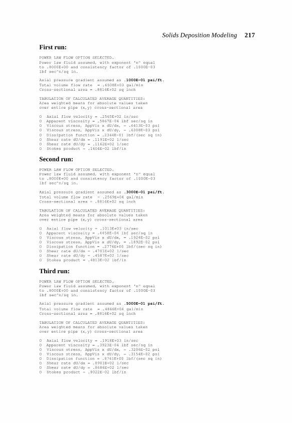
Solids Deposition Modeling 217
First run:
POWER LAW FLOW OPTION SELECTED.Power law fluid assumed, with exponent "n" equalto .8000E+00 and consistency factor of .1000E-03lbf sec^n/sq in.
Axial pressure gradient assumed as .1000E-01 psi/ft.Total volume flow rate = .6508E+03 gal/minCross-sectional area = .8816E+02 sq inch
TABULATION OF CALCULATED AVERAGE QUANTITIES:Area weighted means for absolute values takenover entire pipe (x,y) cross-sectional area
O Axial flow velocity = .2565E+02 in/secO Apparent viscosity = .5867E-04 lbf sec/sq inO Viscous stress, AppVis x dU/dx, = .6413E-03 psiO Viscous stress, AppVis x dU/dy, = .6308E-03 psiO Dissipation function = .2344E-01 lbf/(sec sq in)O Shear rate dU/dx = .1191E+02 1/secO Shear rate dU/dy = .1162E+02 1/secO Stokes product = .1604E-02 lbf/in
Second run:
POWER LAW FLOW OPTION SELECTED.Power law fluid assumed, with exponent "n" equalto .8000E+00 and consistency factor of .1000E-03lbf sec^n/sq in.
Axial pressure gradient assumed as .3000E-01 psi/ft.Total volume flow rate = .2569E+04 gal/minCross-sectional area = .8816E+02 sq inch
TABULATION OF CALCULATED AVERAGE QUANTITIES:Area weighted means for absolute values takenover entire pipe (x,y) cross-sectional area
O Axial flow velocity = .1013E+03 in/secO Apparent viscosity = .4458E-04 lbf sec/sq inO Viscous stress, AppVis x dU/dx, = .1924E-02 psiO Viscous stress, AppVis x dU/dy, = .1892E-02 psiO Dissipation function = .2776E+00 lbf/(sec sq in)O Shear rate dU/dx = .4701E+02 1/secO Shear rate dU/dy = .4587E+02 1/secO Stokes product = .4813E-02 lbf/in
Third run:
POWER LAW FLOW OPTION SELECTED.Power law fluid assumed, with exponent "n" equalto .8000E+00 and consistency factor of .1000E-03lbf sec^n/sq in.
Axial pressure gradient assumed as .5000E-01 psi/ft.
Total volume flow rate = .4866E+04 gal/minCross-sectional area = .8816E+02 sq inch
TABULATION OF CALCULATED AVERAGE QUANTITIES:Area weighted means for absolute values takenover entire pipe (x,y) cross-sectional area
O Axial flow velocity = .1918E+03 in/secO Apparent viscosity = .3923E-04 lbf sec/sq inO Viscous stress, AppVis x dU/dx, = .3206E-02 psiO Viscous stress, AppVis x dU/dy, = .3154E-02 psiO Dissipation function = .8761E+00 lbf/(sec sq in)O Shear rate dU/dx = .8901E+02 1/secO Shear rate dU/dy = .8686E+02 1/secO Stokes product = .8022E-02 lbf/in

218 Computational Rheology
Fourth run:
POWER LAW FLOW OPTION SELECTED.Power law fluid assumed, with exponent "n" equalto .8000E+00 and consistency factor of .1000E-03lbf sec^n/sq in.
Axial pressure gradient assumed as .1000E+00 psi/ft.Total volume flow rate = .1157E+05 gal/minCross-sectional area = .8816E+02 sq inch
TABULATION OF CALCULATED AVERAGE QUANTITIES:Area weighted means for absolute values takenover entire pipe (x,y) cross-sectional area
O Axial flow velocity = .4561E+03 in/secO Apparent viscosity = .3299E-04 lbf sec/sq inO Viscous stress, AppVis x dU/dx, = .6413E-02 psiO Viscous stress, AppVis x dU/dy, = .6308E-02 psiO Dissipation function = .4167E+01 lbf/(sec sq in)O Shear rate dU/dx = .2117E+03 1/secO Shear rate dU/dy = .2066E+03 1/secO Stokes product = .1604E-01 lbf/in
dP/dz (psi/ft)
Vol
ume
Flow
Rat
e (G
PM)
5,000
10,000
0.05 0.100.01
Power Law Model
Figure 8-10. “Q vs. dp/dz” nonlinear behavior.
Simulation 5. Hydrate Plug, Herschel-Bulkley Flow in Circular Duct
In this set of runs, the “large blockage” example in Simulation 4 isreconsidered, with identical parameters, except that a nonzero yield stress of0.005 psi is allowed. Thus, our “power law” fluid model becomes a “Herschel-Bulkley” fluid. Whereas smooth velocity distributions are typical of power lawflows, e.g., Figure 8-9, the velocity field in flows with nonzero yield stress maycontain “plugs” that move as solid bodies. For this simulation set, the plug flowvelocity profiles obtained are typified by Figure 8-11.
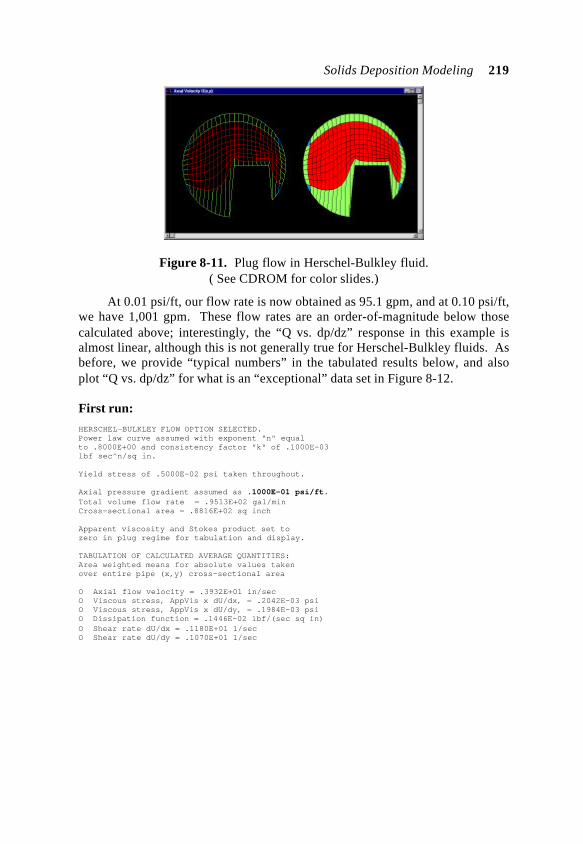
Solids Deposition Modeling 219
Figure 8-11. Plug flow in Herschel-Bulkley fluid.( See CDROM for color slides.)
At 0.01 psi/ft, our flow rate is now obtained as 95.1 gpm, and at 0.10 psi/ft,we have 1,001 gpm. These flow rates are an order-of-magnitude below thosecalculated above; interestingly, the “Q vs. dp/dz” response in this example isalmost linear, although this is not generally true for Herschel-Bulkley fluids. Asbefore, we provide “typical numbers” in the tabulated results below, and alsoplot “Q vs. dp/dz” for what is an “exceptional” data set in Figure 8-12.
First run:
HERSCHEL-BULKLEY FLOW OPTION SELECTED.Power law curve assumed with exponent "n" equalto .8000E+00 and consistency factor "k" of .1000E-03lbf sec^n/sq in.
Yield stress of .5000E-02 psi taken throughout.
Axial pressure gradient assumed as .1000E-01 psi/ft.Total volume flow rate = .9513E+02 gal/minCross-sectional area = .8816E+02 sq inch
Apparent viscosity and Stokes product set tozero in plug regime for tabulation and display.
TABULATION OF CALCULATED AVERAGE QUANTITIES:Area weighted means for absolute values takenover entire pipe (x,y) cross-sectional area
O Axial flow velocity = .3932E+01 in/secO Viscous stress, AppVis x dU/dx, = .2042E-03 psiO Viscous stress, AppVis x dU/dy, = .1984E-03 psiO Dissipation function = .1446E-02 lbf/(sec sq in)O Shear rate dU/dx = .1180E+01 1/secO Shear rate dU/dy = .1070E+01 1/sec
220 Computational Rheology
Second run:
HERSCHEL-BULKLEY FLOW OPTION SELECTED.Power law curve assumed with exponent "n" equalto .8000E+00 and consistency factor "k" of .1000E-03lbf sec^n/sq in.
Yield stress of .5000E-02 psi taken throughout.
Axial pressure gradient assumed as .3000E-01 psi/ft.Total volume flow rate = .2854E+03 gal/minCross-sectional area = .8816E+02 sq inch
Apparent viscosity and Stokes product set tozero in plug regime for tabulation and display.
TABULATION OF CALCULATED AVERAGE QUANTITIES:Area weighted means for absolute values takenover entire pipe (x,y) cross-sectional area
O Axial flow velocity = .1180E+02 in/secO Viscous stress, AppVis x dU/dx, = .6126E-03 psiO Viscous stress, AppVis x dU/dy, = .5951E-03 psiO Dissipation function = .1302E-01 lbf/(sec sq in)O Shear rate dU/dx = .3539E+01 1/secO Shear rate dU/dy = .3211E+01 1/sec
Third run:
HERSCHEL-BULKLEY FLOW OPTION SELECTED.Power law curve assumed with exponent "n" equalto .8000E+00 and consistency factor "k" of .1000E-03lbf sec^n/sq in.
Yield stress of .5000E-02 psi taken throughout.
Axial pressure gradient assumed as .5000E-01 psi/ft.Total volume flow rate = .4757E+03 gal/minCross-sectional area = .8816E+02 sq inch
Apparent viscosity and Stokes product set tozero in plug regime for tabulation and display.
TABULATION OF CALCULATED AVERAGE QUANTITIES:Area weighted means for absolute values takenover entire pipe (x,y) cross-sectional area
O Axial flow velocity = .1966E+02 in/secO Viscous stress, AppVis x dU/dx, = .1021E-02 psiO Viscous stress, AppVis x dU/dy, = .9918E-03 psiO Dissipation function = .3616E-01 lbf/(sec sq in)O Shear rate dU/dx = .5899E+01 1/secO Shear rate dU/dy = .5351E+01 1/sec
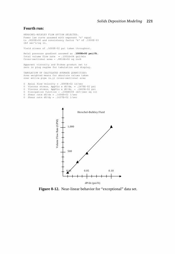
Solids Deposition Modeling 221
Fourth run:
HERSCHEL-BULKLEY FLOW OPTION SELECTED.Power law curve assumed with exponent "n" equalto .8000E+00 and consistency factor "k" of .1000E-03lbf sec^n/sq in.
Yield stress of .5000E-02 psi taken throughout.
Axial pressure gradient assumed as .1000E+00 psi/ft.Total volume flow rate = .1001E+04 gal/minCross-sectional area = .8816E+02 sq inch
Apparent viscosity and Stokes product set tozero in plug regime for tabulation and display.
TABULATION OF CALCULATED AVERAGE QUANTITIES:Area weighted means for absolute values takenover entire pipe (x,y) cross-sectional area
O Axial flow velocity = .4085E+02 in/secO Viscous stress, AppVis x dU/dx, = .2478E-02 psiO Viscous stress, AppVis x dU/dy, = .2463E-02 psiO Dissipation function = .2386E+00 lbf/(sec sq in)O Shear rate dU/dx = .1606E+02 1/secO Shear rate dU/dy = .1637E+02 1/sec
dP/dz (psi/ft)
Vol
ume
Flow
Rat
e (G
PM)
500
1,000
0.05 0.100.01
Herschel-Bulkley Fluid
Figure 8-12. Near-linear behavior for “exceptional” data set.
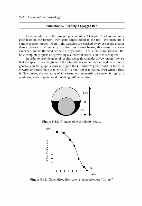
222 Computational Rheology
Simulation 6. Eroding a Clogged Bed
Here, we start with the clogged pipe annulus of Chapter 7, where the innerpipe rests on the bottom, with sand almost filled to the top. We postulate asimple erosion model, where light particles are washed away at speeds greaterthan a given critical velocity. In the runs shown below, this value is alwaysexceeded, so that the sand bed will always erode. In this final simulation set, thehole completely opens up, providing a successful conclusion to this chapter!
In order to provide general results, we again consider a Newtonian flow, sothat the specific results given in the tabulations can be rescaled and recast moregenerally in the graph shown in Figure 8-14. While “Q vs. dp/dz” is linear inNewtonian fluids, note that “Q vs. N” is not. For that matter, even when a flowis Newtonian, the variation of Q versus any geometric parameter is typicallynonlinear, and computational modeling will be required.
N %
100%
Figure 8-13. Clogged pipe simulation setup.
% M
ax V
ol F
low
Rat
e
100%
N
100
Figure 8-14. Generalized flow rate vs. dimensionless “fill-up.”
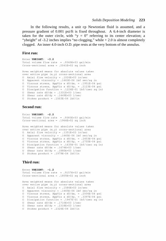
Solids Deposition Modeling 223
In the following results, a unit cp Newtonian fluid is assumed, and apressure gradient of 0.001 psi/ft is fixed throughout. A 6.4-inch diameter istaken for the outer circle, with “y = 0” referring to its center elevation; a“yheight” of -3.2 inches implies “no clogging,” while + 2.0 is almost completelyclogged. An inner 4.0-inch O.D. pipe rests at the very bottom of the annulus.
First run:
Enter YHEIGHT: -3.2Total volume flow rate = .9340E+03 gal/minCross-sectional area = .2041E+02 sq inch
Area weighted means for absolute values takenover entire pipe (x,y) cross-sectional areaO Axial flow velocity = .1026E+03 in/secO Apparent viscosity = .1465E-06 lbf sec/sq inO Viscous stress, AppVis x dU/dx, = .1951E-04 psiO Viscous stress, AppVis x dU/dy, = .2123E-04 psiO Dissipation function = .1226E-01 lbf/(sec sq in)O Shear rate dU/dx = .1331E+03 1/secO Shear rate dU/dy = .1449E+03 1/secO Stokes product = .1503E-04 lbf/in
Second run:
Enter YHEIGHT: -2.2Total volume flow rate = .9383E+03 gal/minCross-sectional area = .1966E+02 sq inch
Area weighted means for absolute values takenover entire pipe (x,y) cross-sectional areaO Axial flow velocity = .1351E+03 in/secO Apparent viscosity = .1465E-06 lbf sec/sq inO Viscous stress, AppVis x dU/dx, = .2453E-04 psiO Viscous stress, AppVis x dU/dy, = .2755E-04 psiO Dissipation function = .1635E-01 lbf/(sec sq in)O Shear rate dU/dx = .1674E+03 1/secO Shear rate dU/dy = .1880E+03 1/secO Stokes product = .1979E-04 lbf/in
Third run:
Enter YHEIGHT: -1.2Total volume flow rate = .9157E+03 gal/minCross-sectional area = .1805E+02 sq inch
Area weighted means for absolute values takenover entire pipe (x,y) cross-sectional areaO Axial flow velocity = .1586E+03 in/secO Apparent viscosity = .1465E-06 lbf sec/sq inO Viscous stress, AppVis x dU/dx, = .2506E-04 psiO Viscous stress, AppVis x dU/dy, = .3397E-04 psiO Dissipation function = .1947E-01 lbf/(sec sq in)O Shear rate dU/dx = .1710E+03 1/secO Shear rate dU/dy = .2318E+03 1/secO Stokes product = .2324E-04 lbf/in
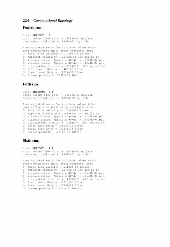
224 Computational Rheology
Fourth run:
Enter YHEIGHT: 0.Total volume flow rate = .7837E+03 gal/minCross-sectional area = .1492E+02 sq inch
Area weighted means for absolute values takenover entire pipe (x,y) cross-sectional areaO Axial flow velocity = .1769E+03 in/secO Apparent viscosity = .1465E-06 lbf sec/sq inO Viscous stress, AppVis x dU/dx, = .1963E-04 psiO Viscous stress, AppVis x dU/dy, = .4324E-04 psiO Dissipation function = .2234E-01 lbf/(sec sq in)O Shear rate dU/dx = .1340E+03 1/secO Shear rate dU/dy = .2951E+03 1/secO Stokes product = .2592E-04 lbf/in
Fifth run:
Enter YHEIGHT: 0.6Total volume flow rate = .6089E+03 gal/minCross-sectional area = .1253E+02 sq inch
Area weighted means for absolute values takenover entire pipe (x,y) cross-sectional areaO Axial flow velocity = .1714E+03 in/secO Apparent viscosity = .1465E-06 lbf sec/sq inO Viscous stress, AppVis x dU/dx, = .1259E-04 psiO Viscous stress, AppVis x dU/dy, = .4737E-04 psiO Dissipation function = .2291E-01 lbf/(sec sq in)O Shear rate dU/dx = .8593E+02 1/secO Shear rate dU/dy = .3233E+03 1/secO Stokes product = .2511E-04 lbf/in
Sixth run:
Enter YHEIGHT: 1.2Total volume flow rate = .2823E+03 gal/minCross-sectional area = .8952E+01 sq inch
Area weighted means for absolute values takenover entire pipe (x,y) cross-sectional areaO Axial flow velocity = .1133E+03 in/secO Apparent viscosity = .1465E-06 lbf sec/sq inO Viscous stress, AppVis x dU/dx, = .8603E-05 psiO Viscous stress, AppVis x dU/dy, = .3692E-04 psiO Dissipation function = .1379E-01 lbf/(sec sq in)O Shear rate dU/dx = .5871E+02 1/secO Shear rate dU/dy = .2520E+03 1/secO Stokes product = .1660E-04 lbf/in
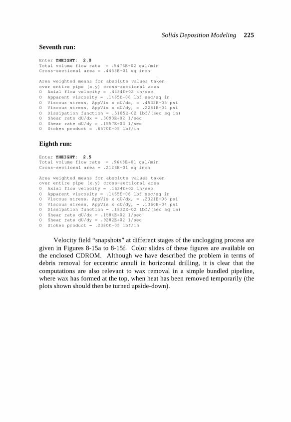
Solids Deposition Modeling 225
Seventh run:
Enter YHEIGHT: 2.0Total volume flow rate = .5476E+02 gal/minCross-sectional area = .4458E+01 sq inch
Area weighted means for absolute values takenover entire pipe (x,y) cross-sectional areaO Axial flow velocity = .4484E+02 in/secO Apparent viscosity = .1465E-06 lbf sec/sq inO Viscous stress, AppVis x dU/dx, = .4532E-05 psiO Viscous stress, AppVis x dU/dy, = .2281E-04 psiO Dissipation function = .5185E-02 lbf/(sec sq in)O Shear rate dU/dx = .3093E+02 1/secO Shear rate dU/dy = .1557E+03 1/secO Stokes product = .6570E-05 lbf/in
Eighth run:
Enter YHEIGHT: 2.5Total volume flow rate = .9648E+01 gal/minCross-sectional area = .2126E+01 sq inch
Area weighted means for absolute values takenover entire pipe (x,y) cross-sectional areaO Axial flow velocity = .1624E+02 in/secO Apparent viscosity = .1465E-06 lbf sec/sq inO Viscous stress, AppVis x dU/dx, = .2321E-05 psiO Viscous stress, AppVis x dU/dy, = .1360E-04 psiO Dissipation function = .1832E-02 lbf/(sec sq in)O Shear rate dU/dx = .1584E+02 1/secO Shear rate dU/dy = .9282E+02 1/secO Stokes product = .2380E-05 lbf/in
Velocity field “snapshots” at different stages of the unclogging process aregiven in Figures 8-15a to 8-15f. Color slides of these figures are available onthe enclosed CDROM. Although we have described the problem in terms ofdebris removal for eccentric annuli in horizontal drilling, it is clear that thecomputations are also relevant to wax removal in a simple bundled pipeline,where wax has formed at the top, when heat has been removed temporarily (theplots shown should then be turned upside-down).
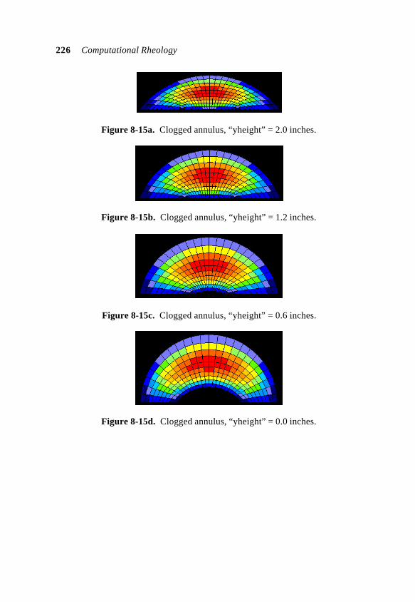
226 Computational Rheology
Figure 8-15a. Clogged annulus, “yheight” = 2.0 inches.
Figure 8-15b. Clogged annulus, “yheight” = 1.2 inches.
Figure 8-15c. Clogged annulus, “yheight” = 0.6 inches.
Figure 8-15d. Clogged annulus, “yheight” = 0.0 inches.
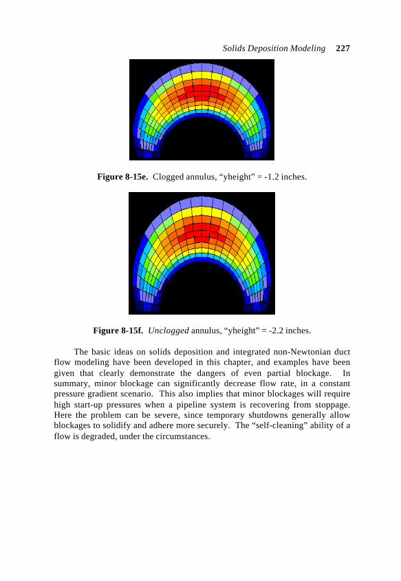
Solids Deposition Modeling 227
Figure 8-15e. Clogged annulus, “yheight” = -1.2 inches.
Figure 8-15f. Unclogged annulus, “yheight” = -2.2 inches.
The basic ideas on solids deposition and integrated non-Newtonian ductflow modeling have been developed in this chapter, and examples have beengiven that clearly demonstrate the dangers of even partial blockage. Insummary, minor blockage can significantly decrease flow rate, in a constantpressure gradient scenario. This also implies that minor blockages will requirehigh start-up pressures when a pipeline system is recovering from stoppage.Here the problem can be severe, since temporary shutdowns generally allowblockages to solidify and adhere more securely. The “self-cleaning” ability of aflow is degraded, under the circumstances.
228 Computational Rheology
REFERENCES
Andersen, M.I, Isaksen, Ø., and Urdahl, O., “Ultrasonic Instrumentation for On-Line Monitoring of Solid Deposition in Pipes,” SPE Paper No. 37437,Production Operations Symposium, Oklahoma City, March 1997.
Anderson, A.G., “Sedimentation,” Handbook of Fluid Mechanics, Streeter, V.L.,Editor, McGraw-Hill, New York, 1961.
Bern, P.A., Withers, V.R., and Cairns, R.J.R., “Wax Deposition in Crude OilPipelines,” EUR Paper No. 206, European Offshore Petroleum Conference andExhibition, London, England, October 1980.
Brown, T.B., Niesen, V.G., and Erickson, D.D., “Measurement and Predictionof the Kinetics of Paraffin Deposition,” SPE Paper No. 26548, SPE AnnualTechnical Conference and Exhibition, Houston, October 1993.
Burger, E.D., Perkins, T.K., and Striegler, J.H., “Studies of Wax Deposition inthe Trans Alaska Pipeline,” SPE Journal of Petroleum Technology, June 1981.
Chang, C., Boger, D.V., and Nguyen, Q.D., “The Yielding of Waxy CrudeOils,” Industrial and Engineering Chemistry Research, Vol. 37, No. 4, 1998, pp.1551-1559.
Chang, C., Boger, D.V., and Nguyen, Q.D., “Influence of Thermal History onthe Waxy Structure of Statically Cooled Waxy Crude Oils,” SPE Paper No.57959, to appear, SPE Journal.
Chang, C., Nguyen, Q.D., and Ronningsen, H.P., “Isothermal Start-Up ofPipeline Transporting Waxy Crude Oil,” Journal of Non-Newtonian FluidMechanics, Vol. 87, 1999, pp. 127-154.
Chen, X.T., Butler, R.A., Volk, M., and Brill, J.P., “Techniques for MeasuringWax Thickness During Single and Multiphase Flow,” SPE Paper No. 38773,SPE Annual Technical Conference and Exhibition, San Antonio, October 1997.
Cussler, E.L., Diffusion Mass Transfer in Fluid Systems, Cambridge UniversityPress, 1997
Elphingstone, G.M., Greenhill, K.L., and Hsu, J.J.C., “Modeling of MultiphaseWax Deposition,” Journal of Energy Resources Technology, Transactions of theASME, Vol. 121, No. 2, June 1999, pp. 81-85.
Forsdyke, I.N., “Flow Assurance in Multiphase Environments,” SPE Paper No.37237, SPE International Symposium on Oilfield Chemistry, Houston, February1996.
Hammami, A., and Raines, M., “Paraffin Deposition from Crude Oils:Comparison of Laboratory Results to Field Data,” SPE Paper No. 38776, SPEAnnual Technical Conference and Exhibition, San Antonio, October 1997.
Henriet, J.P., and Mienert, J., Gas Hydrates: Relevance to World MarginStability and Climatic Change, The Geological Society, London, 1998.
Solids Deposition Modeling 229
Hsu, J.J.C., Santamaria, M.M., and Bribaker, J.P.: “Wax Deposition of WaxyLive Crudes under Turbulent Flow Conditions,” SPE Paper No. 28480, SPEAnnual Technical Conference and Exhibition, New Orleans, September 1994.
Hsu, J.J.C. and Brubaker, J.P., “Wax Deposition Measurement and Scale-UpModeling for Waxy Live Crudes under Turbulent Flow Conditions,” SPE PaperNo. 29976, SPE International Meeting on Petroleum Engineering, Beijing,China, November 1995.
Hsu, J.J.C. and Brubaker, J.P., “Wax Deposition Scale-Up Modeling for WaxyCrude Production Lines,” OTC Paper 7778, Offshore Technology Conference,Houston, May 1995.
Hunt, B.E., “Laboratory Study of Paraffin Deposition,” SPE Journal ofPetroleum Technology, November 1962, pp. 1259-1269.
Ibraheem, S.O., Adewumi, M.A., and Savidge, J.L., “Numerical Simulation ofHydrate Transport in Natural Gas Pipeline,” Journal of Energy ResourcesTechnology, Transactions of the ASME, Vol. 120, March 1998, pp. 20-26.
Jessen F.W. and Howell, J.N., “Effect of Flow Rate on Paraffin Accumulation inPlastic, Steel, and Coated Pipe,” Petroleum Transactions, AIME, 1958, pp. 80-84.
Kapfer, W.H., “Flow of Sludges and Slurries,” Piping Handbook, King, R.,Editor, McGraw-Hill, New York, 1973.
Keating, J.F., and Wattenbarger, R.A., “The Simulation of Paraffin Depositionand Removal in Wellbores,” SPE Paper No. 27871, SPE Western RegionalMeeting, Long Beach, California, March 1994.
Majeed, A., Bringedal, B., and Overa, S., “Model Calculates Wax Depositionfor North Sea Oils,” Oil and Gas Journal, June 1990, pp. 63-69.
Matzain, A., “Single Phase Liquid Paraffin Deposition Modeling,” MS Thesis,The University of Tulsa, Tulsa, Oklahoma, 1996.
Mendes, P.R.S. and Braga, S.L., “Obstruction of Pipelines during the Flow ofWaxy Crude Oils,” Journal of Fluids Engineering, Transactions of the ASME,December 1996, pp. 722-728.
Pate, C.B., “MMS/Deepstar Workshop on Produced Fluids,” OffshoreTechnology Conference, Houston, May 1995.
Shauly, A., Wachs, A., and Nir, A., “Shear-Induced Particle Resuspension inSettling Polydisperse Concentrated Suspension,” International Journal ofMultiphase Flow, Vol. 26, 2000, pp. 1-15.
Singh P., Fogler H.S., and Nagarajan N., “Prediction of the Wax Content of theIncipient Wax-Oil Gel in a Pipeline: An Application of the Controlled-StressRheometer,” Journal of Rheology, Vol. 43, No. 6, November-December 1999,pp. 1437-1459.
230 Computational Rheology
Souza Mendes, P.R., Braga, A.M.B., Azevedo, L.F.A., and Correa, K.S.,“Resistive Force of Wax Deposits During Pigging Operations,” Journal ofEnergy Resources Technology, Transactions of the ASME, Vol. 121, September1999, pp. 167-171.
Wardhaugh, L.T., and Boger, D.V. “Flow Characteristics of Waxy Crude Oils:Application to Pipeline Design,” AIChE Journal, Vol. 37, No. 6 June 1991, pp.871-885.
Weingarten J.S., and Euchner, J.A., “Methods for Predicting Wax Precipitationand Deposition,” SPE Journal of Production Engineering, February 1988, pp.121-126.
231
9
Pipe Bends, Secondary Flows,and Fluid Heterogeneities
In this chapter, we develop the mathematical ideas needed to model flow inslow pipe bends, that is, in pipelines where the radius of curvature of the axissignificantly exceeds duct cross-dimensions; in this limit, the correctionsaccount for centrifugal effects only. For smaller radii of curvature, secondaryviscous flows in the cross-plane appear, in addition to centrifugal effects; theseare already discussed in experimental literature and are not reconsidered here.
Why study the large radius limit? In many drilling and subsea pipelineapplications, slow geometric change along the axis is the rule, and secondaryviscous flows are not anticipated. But when drillstrings turn horizontally, orwhen pipelines bend over mounds, flow differences at the top and bottom of thecross-section may initiate pipe blockage. Centrifugal effects may be associatedwith debris accumulations, not unlike observed preferential soil depositionoccurring at selected sides of meandering river channels. How does solidsdeposition take place? Can local stress fields remove this debris?
These questions are eliciting interest from subsea pipeline engineersstudying wax, hydrate, asphaltene, and sand removal. Thus, the calculation ofvelocity, shear rate, viscous stress and pressure drop for non-Newtonian flow inarbitrary ducts, in particular, clogged ducts, is important, and especially tosteady-state and start-up operations. The work of this chapter, emphasizing theeffects of bends, aims at supporting ongoing deposition studies. In the sameway that different deposition mechanisms govern “cohesive” versus “non-cohesive particles” in sedimentary transport, we anticipate that different lawsapply to different types of debris. Our methods use laboratory “n, k” data topredict field scale rheological properties, hopeful that these parameters willprovide meaningful correlation variables for pipe clog prediction.

232 Computational Rheology
MODELING NON-NEWTONIAN DUCT FLOW IN PIPE BENDS
Bends in pipelines and annuli are interesting because they are associatedwith losses; that is, to maintain a prescribed volume flow rate, a greater pressuredrop is required in pipes with bends than those without. This is true because theviscous stresses that act along pipe walls are higher. We will discuss theproblem analytically, in the context of Newtonian flow; in this limit, exactsolutions are derived for Poiseuille flow between curved concentric plates, butwe will also focus on the form of the new differential equation used. The closedform expressions for Newtonian flow derived are new. Their derivationmotivates our methodology for non-Newtonian flows in three-dimensional,curved, closed ducts, which can only be analyzed computationally.
xy
Figure 9-1a. Viscous flow in a circular pipe.
xy
Figure 9-1b. Viscous flow in a rectangular duct.
xy
Figure 9-1c. Viscous flow in general duct.
Straight, closed ducts. We have so far derived analytical solutions forNewtonian flows in straight circular and rectangular conduits, as shown inFigures 9-1a and 9-1b. We also developed a general non-Newtonian viscousflow solver applicable to arbitrary straight ducts, e.g., see Figure 9-1c, utilizingcurvilinear meshes, which supplements the algorithm of Chapter 2 applicable toeccentric annuli. For both ducts and annuli, we have demonstrated that the
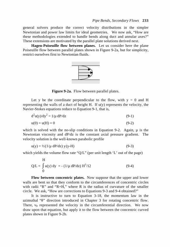
Pipe Bends, Secondary Flows 233
general solvers produce the correct velocity distributions in the simplerNewtonian and power law limits for ideal geometries. We now ask, “How arethese methodologies extended to handle bends along duct and annular axes?”These extensions are motivated by the parallel plate solutions derived next.
Hagen-Poiseuille flow between planes. Let us consider here the planePoiseuille flow between parallel plates shown in Figure 9-2a, but for simplicity,restrict ourselves first to Newtonian fluids.
Figure 9-2a. Flow between parallel plates.
Let y be the coordinate perpendicular to the flow, with y = 0 and Hrepresenting the walls of a duct of height H. If u(y) represents the velocity, theNavier-Stokes equations reduce to Equation 9-1, that is,
d2u(y)/dy2 = 1/µ dP/dz (9-1)
u(0) = u(H) = 0 (9-2)
which is solved with the no-slip conditions in Equation 9-2. Again, µ is theNewtonian viscosity and dP/dz is the constant axial pressure gradient. Thevelocity solution is the well-known parabolic profile
u(y) = ½ (1/µ dP/dz) y (y-H) (9-3)
which yields the volume flow rate “Q/L” (per unit length ‘L’ out of the page)
H
Q/L = ∫ u(y) dy = - (1/µ dP/dz) H3/12 (9-4)0
Flow between concentric plates. Now suppose that the upper and lowerwalls are bent so that they conform to the circumferences of concentric circleswith radii “R” and “R+H,” where R is the radius of curvature of the smallercircle. We ask, “How are corrections to Equations 9-3 and 9-4 obtained?”
It is instructive to turn to Equation 3-18, the momentum law in theazimuthal “θ” direction introduced in Chapter 3 for rotating concentric flow.There, vθ represented the velocity in the circumferential direction. We nowdraw upon that equation, but apply it to the flow between the concentric curvedplates shown in Figure 9-2b.

234 Computational Rheology
Rc
Figure 9-2b. Opened duct flow between concentric curved plates.
Since there is no flow perpendicular to the page, vz = 0; also, vr = 0because the velocity is directed only tangentially, and Fθ is assumed to be zero.In these coordinates, the flow is steady, and θ and “z” variations vanishidentically. Thus, Equation 3-18 reduces to the ordinary differential equation
d 2vθ /dr
2 + 1/r dvθ /dr - vθ /r 2 = 1/µ 1/r dP/dθ (9-5)
where the right side, containing the axial pressure gradient “1/r dP/dθ,” isapproximately constant. It must be solved together with the no-slip conditions
vθ(R) = vθ(R+H) = 0 (9-6)
A closed form solution can be obtained as
vθ(r)/[1/µ 1/r dP/dθ] = (R+H)3 - R3/R2 - (R+H)2 × (r/3)- R2(R+H)2/R2 - (R+H)2 × H/(3r) + 1/3 r2 (9-7)
Then, the volume flow rate “Q/L” per unit length (out of the page) is easilycomputed from
R+H
Q/L = ∫ vθ(r) dr (9-8)R
exactly as
Q/L = ( 1/18) (1/µ dP/dz) (9-9)
- 6R3H - 9R2H2 - 5RH3 - H4 + 6R4 ln(R+H)
+ 12HR3 ln(R+H) + 6H2R2 ln(R+H) - 6R4 ln(R)
- 12R3H ln(R) - 6R2H2 ln(R)/(2R+H)
where we have replaced “1/r dP/dθ” by “dP/dz.” Now, in the limit R >> H,Equation 9-9 simplifies to
Q/L ≈ (1/µ dP/dz) - H3/12 + H5/(180 R2) + O(1/R3 ) (9-10)
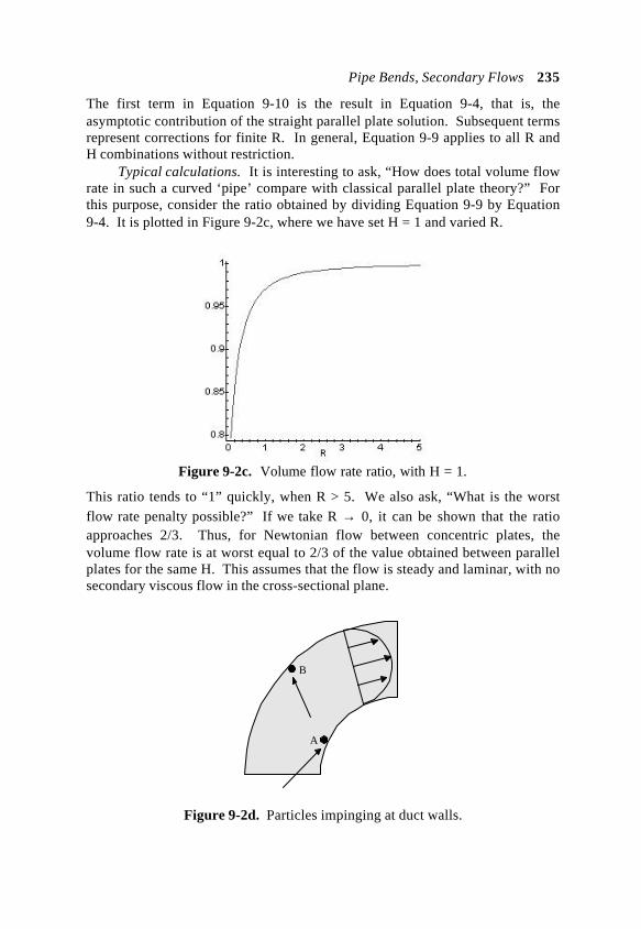
Pipe Bends, Secondary Flows 235
The first term in Equation 9-10 is the result in Equation 9-4, that is, theasymptotic contribution of the straight parallel plate solution. Subsequent termsrepresent corrections for finite R. In general, Equation 9-9 applies to all R andH combinations without restriction.
Typical calculations. It is interesting to ask, “How does total volume flowrate in such a curved ‘pipe’ compare with classical parallel plate theory?” Forthis purpose, consider the ratio obtained by dividing Equation 9-9 by Equation9-4. It is plotted in Figure 9-2c, where we have set H = 1 and varied R.
Figure 9-2c. Volume flow rate ratio, with H = 1.
This ratio tends to “1” quickly, when R > 5. We also ask, “What is the worstflow rate penalty possible?” If we take R → 0, it can be shown that the ratioapproaches 2/3. Thus, for Newtonian flow between concentric plates, thevolume flow rate is at worst equal to 2/3 of the value obtained between parallelplates for the same H. This assumes that the flow is steady and laminar, with nosecondary viscous flow in the cross-sectional plane.
A
B
Figure 9-2d. Particles impinging at duct walls.
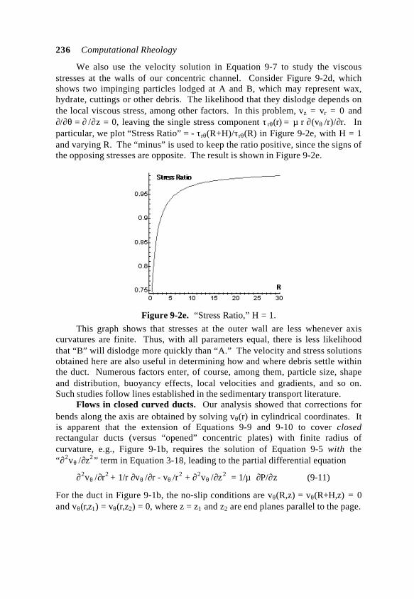
236 Computational Rheology
We also use the velocity solution in Equation 9-7 to study the viscousstresses at the walls of our concentric channel. Consider Figure 9-2d, whichshows two impinging particles lodged at A and B, which may represent wax,hydrate, cuttings or other debris. The likelihood that they dislodge depends onthe local viscous stress, among other factors. In this problem, vz = vr = 0 and∂/∂θ = ∂ /∂z = 0, leaving the single stress component τ rθ(r) = µ r ∂ (vθ /r)/∂r. Inparticular, we plot “Stress Ratio” = - τ rθ(R+H)/τ rθ(R) in Figure 9-2e, with H = 1and varying R. The “minus” is used to keep the ratio positive, since the signs ofthe opposing stresses are opposite. The result is shown in Figure 9-2e.
Figure 9-2e. “Stress Ratio,” H = 1.
This graph shows that stresses at the outer wall are less whenever axiscurvatures are finite. Thus, with all parameters equal, there is less likelihoodthat “B” will dislodge more quickly than “A.” The velocity and stress solutionsobtained here are also useful in determining how and where debris settle withinthe duct. Numerous factors enter, of course, among them, particle size, shapeand distribution, buoyancy effects, local velocities and gradients, and so on.Such studies follow lines established in the sedimentary transport literature.
Flows in closed curved ducts. Our analysis showed that corrections forbends along the axis are obtained by solving vθ(r) in cylindrical coordinates. Itis apparent that the extension of Equations 9-9 and 9-10 to cover closedrectangular ducts (versus “opened” concentric plates) with finite radius ofcurvature, e.g., Figure 9-1b, requires the solution of Equation 9-5 with the“∂
2vθ /∂z 2
” term in Equation 3-18, leading to the partial differential equation
∂ 2vθ /∂r
2 + 1/r ∂vθ /∂r - vθ /r 2 + ∂
2vθ /∂z 2 = 1/µ ∂P/∂z (9-11)
For the duct in Figure 9-1b, the no-slip conditions are vθ(R,z) = vθ(R+H,z) = 0and vθ(r,z1) = vθ(r,z2) = 0, where z = z1 and z2 are end planes parallel to the page.
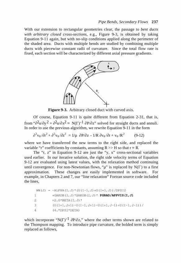
Pipe Bends, Secondary Flows 237
With our extension to rectangular geometries clear, the passage to bent ductswith arbitrary closed cross-sections, e.g., Figure 9-3, is obtained by takingEquation 9-11 again, but with no-slip conditions applied along the perimeter ofthe shaded area. Ducts with multiple bends are studied by combining multipleducts with piecewise constant radii of curvature. Since the total flow rate isfixed, each section will be characterized by different axial pressure gradients.
Rc
x
y
Figure 9-3. Arbitrary closed duct with curved axis.
Of course, Equation 9-11 is quite different from Equation 2-31, that is,
from “∂2u/∂y2 + ∂2u/∂x2 ≈ N(Γ)-1 ∂P/∂z” solved for straight ducts and annuli.In order to use the previous algorithm, we rewrite Equation 9-11 in the form
∂ 2vθ /∂r
2 + ∂ 2vθ /∂z
2 = 1/µ ∂P/∂z - 1/R ∂vθ /∂r + vθ /R 2 (9-12)
where we have transferred the new terms to the right side, and replaced thevariable “r” coefficients by constants, assuming R >> H so that r ≈ R.
The “r, z” in Equation 9-12 are just the “y, x” cross-sectional variablesused earlier. In our iterative solution, the right side velocity terms of Equation9-12 are evaluated using latest values, with the relaxation method continuinguntil convergence. For non-Newtonian flows, “µ” is replaced by N(Γ) to a firstapproximation. These changes are easily implemented in software. Forexample, in Chapters 2 and 7, our “line relaxation” Fortran source code includedthe lines,
WW(J) = -ALPHA(I,J)*(U(I-1,J)+U(I+1,J))/DPSI2
1 +GAKOB(I,J)*GAKOB(I,J)* PGRAD/APPVIS(I,J)
2 +2.0*BETA(I,J)*
3 (U(I+1,J+1)-U(I-1,J+1)-U(I+1,J-1)+U(I-1,J-1))/
4 (4.*DPSI*DETA)
which incorporate “N(Γ)-1 ∂P/∂z,” where the other terms shown are related tothe Thompson mapping. To introduce pipe curvature, the bolded term is simplyreplaced as follows,
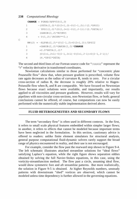
238 Computational Rheology
CHANGE = PGRAD/APPVIS(I,J)
1 -(YETA(I,J)*(U(I+1,J)-U(I-1,J))/(2.*DPSI)
2 - YPSI(I,J)*(U(I,J+1)-U(I,J-1))/(2.*DETA))/
3 (GAKOB(I,J)*RCURV)
4 + U(I,J)/(RCURV**2.)C WW(J) = -ALPHA(I,J)*(U(I-1,J)+U(I+1,J))/DPSI2
1 +GAKOB(I,J)*GAKOB(I,J)*CHANGE
2 +2.0*BETA(I,J)*
3 (U(I+1,J+1)-U(I-1,J+1)-U(I+1,J-1)+U(I-1,J-1))/
4 (4.*DPSI*DETA)
The second and third lines of our Fortran source code for “CHANGE” represent the“r” velocity derivative in transformed coordinates.
Newtonian calculations similar to those performed for “concentric platePouseuille flow” show that, when pressure gradient is prescribed, volume flowrate again decreases as the radius of curvature Rc tends to zero. For a circularcross-section of radius R, the decrease is roughly 20% relative to Hagen-Poiseuille flow when Rc and R are comparable. We have focused on Newtonianflows because exact solutions were available, and importantly, our resultsapplied to all viscosities and pressure gradients. However, results will vary forpipelines with non-circular cross-sections, non-Newtonian flow, or both; generalconclusions cannot be offered, of course, but computations can now be easilyperformed with the numerically stable implementation derived above.
FLUID HETEROGENEITIES AND SECONDARY FLOWS
The term “secondary flow” is often used in different contexts. In the first,it refers to small scale physical features embedded within simpler larger flows;in another, it refers to effects that cannot be modeled because important termshave been neglected in the formulation. In this section, cautionary advice isoffered to readers: unlike finite element simulators for structural analysis,general purpose computational fluid-dynamic solvers rarely support the broadrange of physics encountered in reality, and their use is not encouraged.
For example, consider the flow past the rearward step shown in Figure 9-4.The left schematic illustrates attached streamline solutions for “ideal flows”satisfying Laplace’s equation, while the right figure shows separation eddiesobtained by solving the full Navier-Stokes equations, in this case, using thevorticity-streamfunction method. The flow past a circle, assuming ideal flow,would show symmetric fore and aft streamline patterns. But more realistically,the solution in Figure 9-5 is obtained. At higher Reynolds numbers, unsteadypatterns with downstream “shed” vortices are observed, which cannot bemodeled unless time dependency is further allowed in the governing equations.
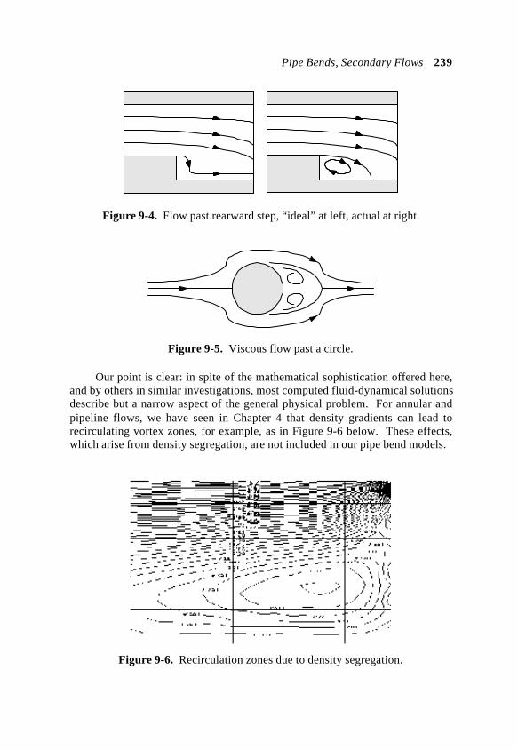
Pipe Bends, Secondary Flows 239
Figure 9-4. Flow past rearward step, “ideal” at left, actual at right.
Figure 9-5. Viscous flow past a circle.
Our point is clear: in spite of the mathematical sophistication offered here,and by others in similar investigations, most computed fluid-dynamical solutionsdescribe but a narrow aspect of the general physical problem. For annular andpipeline flows, we have seen in Chapter 4 that density gradients can lead torecirculating vortex zones, for example, as in Figure 9-6 below. These effects,which arise from density segregation, are not included in our pipe bend models.
Figure 9-6. Recirculation zones due to density segregation.
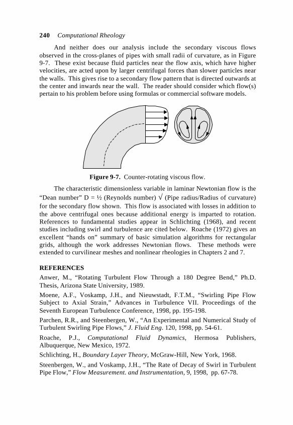
240 Computational Rheology
And neither does our analysis include the secondary viscous flowsobserved in the cross-planes of pipes with small radii of curvature, as in Figure9-7. These exist because fluid particles near the flow axis, which have highervelocities, are acted upon by larger centrifugal forces than slower particles nearthe walls. This gives rise to a secondary flow pattern that is directed outwards atthe center and inwards near the wall. The reader should consider which flow(s)pertain to his problem before using formulas or commercial software models.
Figure 9-7. Counter-rotating viscous flow.
The characteristic dimensionless variable in laminar Newtonian flow is the“Dean number” D = ½ (Reynolds number) √ (Pipe radius/Radius of curvature)for the secondary flow shown. This flow is associated with losses in addition tothe above centrifugal ones because additional energy is imparted to rotation.References to fundamental studies appear in Schlichting (1968), and recentstudies including swirl and turbulence are cited below. Roache (1972) gives anexcellent “hands on” summary of basic simulation algorithms for rectangulargrids, although the work addresses Newtonian flows. These methods wereextended to curvilinear meshes and nonlinear rheologies in Chapters 2 and 7.
REFERENCES
Anwer, M., “Rotating Turbulent Flow Through a 180 Degree Bend,” Ph.D.Thesis, Arizona State University, 1989.
Moene, A.F., Voskamp, J.H., and Nieuwstadt, F.T.M., “Swirling Pipe FlowSubject to Axial Strain,” Advances in Turbulence VII. Proceedings of theSeventh European Turbulence Conference, 1998, pp. 195-198.
Parchen, R.R., and Steenbergen, W., “An Experimental and Numerical Study ofTurbulent Swirling Pipe Flows,” J. Fluid Eng. 120, 1998, pp. 54-61.
Roache, P.J., Computational Fluid Dynamics, Hermosa Publishers,Albuquerque, New Mexico, 1972.
Schlichting, H., Boundary Layer Theory, McGraw-Hill, New York, 1968.
Steenbergen, W., and Voskamp, J.H., “The Rate of Decay of Swirl in TurbulentPipe Flow,” Flow Measurement. and Instrumentation, 9, 1998, pp. 67-78.
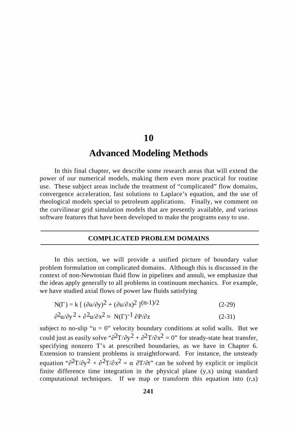
241
10
Advanced Modeling Methods
In this final chapter, we describe some research areas that will extend thepower of our numerical models, making them even more practical for routineuse. These subject areas include the treatment of “complicated” flow domains,convergence acceleration, fast solutions to Laplace’s equation, and the use ofrheological models special to petroleum applications. Finally, we comment onthe curvilinear grid simulation models that are presently available, and varioussoftware features that have been developed to make the programs easy to use.
COMPLICATED PROBLEM DOMAINS
In this section, we will provide a unified picture of boundary valueproblem formulation on complicated domains. Although this is discussed in thecontext of non-Newtonian fluid flow in pipelines and annuli, we emphasize thatthe ideas apply generally to all problems in continuum mechanics. For example,we have studied axial flows of power law fluids satisfying
N(Γ) = k [ (∂u/∂y)2 + (∂u/∂x)2 ](n-1)/2 (2-29)
∂2u/∂y2 + ∂2u/∂x2 ≈ N(Γ)-1 ∂P/∂z (2-31)
subject to no-slip “u = 0” velocity boundary conditions at solid walls. But we
could just as easily solve “∂2T/∂y2 + ∂2T/∂x2 = 0” for steady-state heat transfer,specifying nonzero T’s at prescribed boundaries, as we have in Chapter 6.Extension to transient problems is straightforward. For instance, the unsteady
equation “∂2T/∂y2 + ∂2T/∂x2 = α ∂T/∂t” can be solved by explicit or implicitfinite difference time integration in the physical plane (y,x) using standardcomputational techniques. If we map or transform this equation into (r,s)
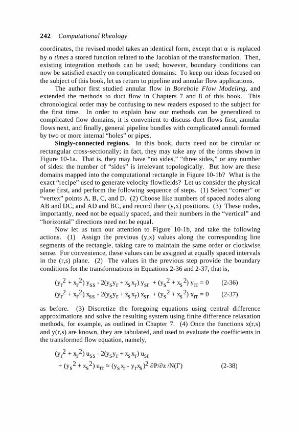
242 Computational Rheology
coordinates, the revised model takes an identical form, except that α is replacedby α times a stored function related to the Jacobian of the transformation. Then,existing integration methods can be used; however, boundary conditions cannow be satisfied exactly on complicated domains. To keep our ideas focused onthe subject of this book, let us return to pipeline and annular flow applications.
The author first studied annular flow in Borehole Flow Modeling, andextended the methods to duct flow in Chapters 7 and 8 of this book. Thischronological order may be confusing to new readers exposed to the subject forthe first time. In order to explain how our methods can be generalized tocomplicated flow domains, it is convenient to discuss duct flows first, annularflows next, and finally, general pipeline bundles with complicated annuli formedby two or more internal “holes” or pipes.
Singly-connected regions. In this book, ducts need not be circular orrectangular cross-sectionally; in fact, they may take any of the forms shown inFigure 10-1a. That is, they may have “no sides,” “three sides,” or any numberof sides: the number of “sides” is irrelevant topologically. But how are thesedomains mapped into the computational rectangle in Figure 10-1b? What is theexact “recipe” used to generate velocity flowfields? Let us consider the physicalplane first, and perform the following sequence of steps. (1) Select “corner” or“vertex” points A, B, C, and D. (2) Choose like numbers of spaced nodes alongAB and DC, and AD and BC, and record their (y,x) positions. (3) These nodes,importantly, need not be equally spaced, and their numbers in the “vertical” and“horizontal” directions need not be equal.
Now let us turn our attention to Figure 10-1b, and take the followingactions. (1) Assign the previous (y,x) values along the corresponding linesegments of the rectangle, taking care to maintain the same order or clockwisesense. For convenience, these values can be assigned at equally spaced intervalsin the (r,s) plane. (2) The values in the previous step provide the boundaryconditions for the transformations in Equations 2-36 and 2-37, that is,
(yr2 + xr
2) yss - 2(ysyr + xs xr) ysr + (ys2 + xs
2) yrr = 0 (2-36)
(yr2 + xr
2) xss - 2(ysyr + xs xr) xsr + (ys2 + xs
2) xrr = 0 (2-37)
as before. (3) Discretize the foregoing equations using central differenceapproximations and solve the resulting system using finite difference relaxationmethods, for example, as outlined in Chapter 7. (4) Once the functions x(r,s)and y(r,s) are known, they are tabulated, and used to evaluate the coefficients inthe transformed flow equation, namely,
(yr2 + xr
2) uss - 2(ysyr + xs xr) usr
+ (ys2 + xs
2) urr ≈ (ys xr - yrxs )2 ∂P/∂z /N(Γ) (2-38)
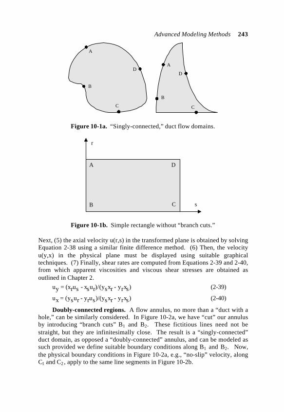
Advanced Modeling Methods 243
A
B
A
B
C
DD
C
Figure 10-1a. “Singly-connected,” duct flow domains.
DA
B C
r
s
Figure 10-1b. Simple rectangle without “branch cuts.”
Next, (5) the axial velocity u(r,s) in the transformed plane is obtained by solvingEquation 2-38 using a similar finite difference method. (6) Then, the velocityu(y,x) in the physical plane must be displayed using suitable graphicaltechniques. (7) Finally, shear rates are computed from Equations 2-39 and 2-40,from which apparent viscosities and viscous shear stresses are obtained asoutlined in Chapter 2.
uy = (xrus - xsur)/(ysxr - yrxs) (2-39)
ux = (ysur - yrus)/(ysxr - yrxs) (2-40)
Doubly-connected regions. A flow annulus, no more than a “duct with ahole,” can be similarly considered. In Figure 10-2a, we have “cut” our annulusby introducing “branch cuts” B1 and B2. These fictitious lines need not bestraight, but they are infinitesimally close. The result is a “singly-connected”duct domain, as opposed a “doubly-connected” annulus, and can be modeled assuch provided we define suitable boundary conditions along B1 and B2. Now,the physical boundary conditions in Figure 10-2a, e.g., “no-slip” velocity, alongC1 and C2 , apply to the same line segments in Figure 10-2b.
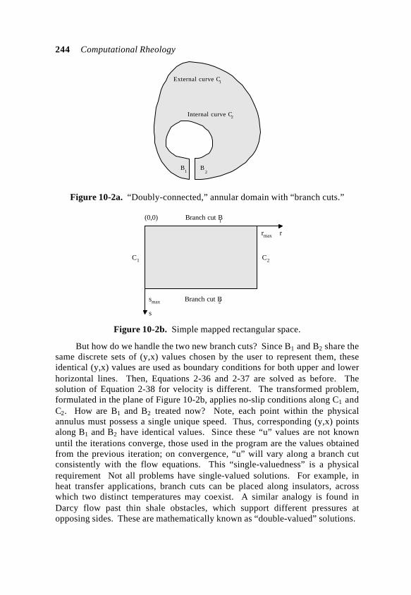
244 Computational Rheology
External curve C1
Internal curve C2
B1
B2
Figure 10-2a. “Doubly-connected,” annular domain with “branch cuts.”
(0,0) Branch cut B1
smax Branch cut B2
C1 C2
rmax r
s
Figure 10-2b. Simple mapped rectangular space.
But how do we handle the two new branch cuts? Since B1 and B2 share thesame discrete sets of (y,x) values chosen by the user to represent them, theseidentical (y,x) values are used as boundary conditions for both upper and lowerhorizontal lines. Then, Equations 2-36 and 2-37 are solved as before. Thesolution of Equation 2-38 for velocity is different. The transformed problem,formulated in the plane of Figure 10-2b, applies no-slip conditions along C1 andC2. How are B1 and B2 treated now? Note, each point within the physicalannulus must possess a single unique speed. Thus, corresponding (y,x) pointsalong B1 and B2 have identical values. Since these “u” values are not knownuntil the iterations converge, those used in the program are the values obtainedfrom the previous iteration; on convergence, “u” will vary along a branch cutconsistently with the flow equations. This “single-valuedness” is a physicalrequirement Not all problems have single-valued solutions. For example, inheat transfer applications, branch cuts can be placed along insulators, acrosswhich two distinct temperatures may coexist. A similar analogy is found inDarcy flow past thin shale obstacles, which support different pressures atopposing sides. These are mathematically known as “double-valued” solutions.
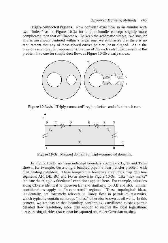
Advanced Modeling Methods 245
Triply-connected regions. Now consider axial flow in an annulus withtwo “holes,” as in Figure 10-3a for a pipe bundle concept slightly morecomplicated than that of Chapter 6. To keep the schematic simple, two smallercircles are shown centered within a larger one; we emphasize that there is norequirement that any of these closed curves be circular or aligned. As in theprevious example, our approach is the use of “branch cuts” that transform theproblem into one for simple duct flow, as Figure 10-3b clearly shows.
ABCD
E F G H
T1
T2T3
Figure 10-3a,b. “Triply-connected” region, before and after branch cuts.
A
B C D E F G
H
T3
r
s
T2T3
T1
Figure 10-3c. Mapped domain for triply-connected domains.
In Figure 10-3b, we have indicated boundary conditions T1, T2 and T3 asshown, for example, describing a bundled pipeline heat transfer problem withdual heating cylinders. These temperature boundary conditions map into linesegments AH, DE, BC, and FG as shown in Figure 10-3c. Like “tick marks”indicate the “single-valuedness” conditions applied here. For example, solutionsalong CD are identical to those on EF, and similarly, for AB and HG. Similarconsiderations apply to “n-connected” regions. These topological ideas,incidentally, are extremely relevant to Darcy flow in petroleum reservoirs,which typically contain numerous “holes,” otherwise known as oil wells. In thiscontext, we emphasize that boundary conforming, curvilinear meshes permitdetailed flow resolution, more than enough to resolve the local logarithmicpressure singularities that cannot be captured on cruder Cartesian meshes.
246 Computational Rheology
CONVERGENCE ACCELERATION
Here we discuss fast methods for irregular grid generation. Existingsolution methods solving x(r,s) and y(r,s) “stagger” the solutions for Equations2-36 and 2-37. Crude solutions are used to initialize the coefficients of Equation2-36, and improvements to x(r,s) are obtained. These are used to evaluate thecoefficients of Equation 2-37, in order to obtain an improved y(r,s); then,attention turns to Equation 2-36 again, and so on, until convergence is achieved.
Various means are used to implement these iterations, as noted in thereview paper of Thompson (1984), e.g., “point SOR,” “line SLOR,” “line SORwith explicit damping,” “alternating-direction-implicit,” and “multigrid,” withvarying degrees of success. Often these schemes diverge computationally. Inany event, the “staggering” noted above introduces different “artificial timelevels” while iterating, however, classic numerical analysis suggests that fasterconvergence and improved stability is possible by reducing their number.
A new approach to solve Thompson’s equations rapidly was proposed byChin (2000) and based on a very simple idea. Consider “zrr + zss = 0,” for which“zi,j ≈ (zi-1,j + zi+1,j + zi,j-1 + zi,j+1)/4” holds on constant grids. This
averaging law was derived earlier for flow in rectangular ducts. It motivates the
recursion formula zi,jn = (zi-1,j
n-1 + zi+1,jn-1 + zi,j-1
n-1 + zi,j+1n-1)/4 often
used to illustrate and develop “multi-level” iterative solutions; an approximate,and even trivial solution, can be used to initialize the calculations, and nonzerosolutions are always produced from nonzero boundary conditions.
But the well known Gauss-Seidel method is fastest: as soon as a new valueof zi,j is calculated, its previous value is discarded and overwritten by the new
value. This speed is accompanied by low memory requirements, since there isno need to store both “n” and “n-1” level solutions: only a single array, zi,jitself, is required in programming. Our new approach to Equations 2-36 and 37was motivated by this simple idea. Rather than solving for x(r,s) and y(r,s) in a“staggered, leap-frog” manner, is it possible to update x and y simultaneously ina similar “once only” manner? Is convergence significantly increased? How dowe solve in Gauss-Seidel fashion? What are the programming implications?
Complex variables provides the vehicle. We define a dependent variable“z” by z(r,s) = x(r,s) + i y(r,s), in particular, adding Equation 2-36 plus i times
Equation 2-37, to obtain (xr2 + yr
2) zss – 2 (xs xr + ysyr) zsr + (xs2 + ys
2) zrr = 0.
Now, the “complex conjugate” of “z” is z*(r,s) = x(r,s) - i y(r,s), from which we
find x = (z + z*)/2 and y = - i (z - z*)/2. Substitution produces the simple andequivalent “one equation” result
(zr zr*) zss - (zs zr
* + zs*zr ) zsr + (zs zs
*) zrr = 0 (10-1)
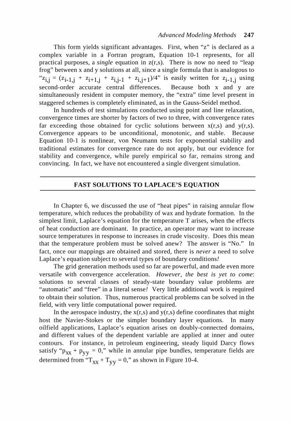
Advanced Modeling Methods 247
This form yields significant advantages. First, when “z” is declared as acomplex variable in a Fortran program, Equation 10-1 represents, for allpractical purposes, a single equation in z(r,s). There is now no need to “leapfrog” between x and y solutions at all, since a single formula that is analogous to“zi,j = (zi-1,j + zi+1,j + zi,j-1 + zi,j+1)/4” is easily written for zi-1,j using
second-order accurate central differences. Because both x and y aresimultaneously resident in computer memory, the “extra” time level present instaggered schemes is completely eliminated, as in the Gauss-Seidel method.
In hundreds of test simulations conducted using point and line relaxation,convergence times are shorter by factors of two to three, with convergence ratesfar exceeding those obtained for cyclic solutions between x(r,s) and y(r,s).Convergence appears to be unconditional, monotonic, and stable. BecauseEquation 10-1 is nonlinear, von Neumann tests for exponential stability andtraditional estimates for convergence rate do not apply, but our evidence forstability and convergence, while purely empirical so far, remains strong andconvincing. In fact, we have not encountered a single divergent simulation.
FAST SOLUTIONS TO LAPLACE’S EQUATION
In Chapter 6, we discussed the use of “heat pipes” in raising annular flowtemperature, which reduces the probability of wax and hydrate formation. In thesimplest limit, Laplace’s equation for the temperature T arises, when the effectsof heat conduction are dominant. In practice, an operator may want to increasesource temperatures in response to increases in crude viscosity. Does this meanthat the temperature problem must be solved anew? The answer is “No.” Infact, once our mappings are obtained and stored, there is never a need to solveLaplace’s equation subject to several types of boundary conditions!
The grid generation methods used so far are powerful, and made even moreversatile with convergence acceleration. However, the best is yet to come:solutions to several classes of steady-state boundary value problems are“automatic” and “free” in a literal sense! Very little additional work is requiredto obtain their solution. Thus, numerous practical problems can be solved in thefield, with very little computational power required.
In the aerospace industry, the x(r,s) and y(r,s) define coordinates that mighthost the Navier-Stokes or the simpler boundary layer equations. In manyoilfield applications, Laplace’s equation arises on doubly-connected domains,and different values of the dependent variable are applied at inner and outercontours. For instance, in petroleum engineering, steady liquid Darcy flowssatisfy “pxx + pyy = 0,” while in annular pipe bundles, temperature fields are
determined from “Txx + Tyy = 0,” as shown in Figure 10-4.
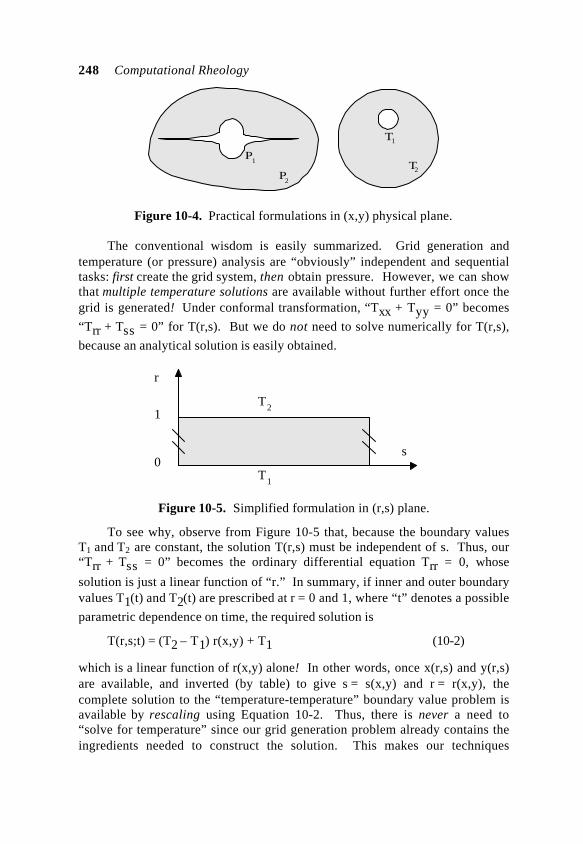
248 Computational Rheology
P2
P1
T1
T2
Figure 10-4. Practical formulations in (x,y) physical plane.
The conventional wisdom is easily summarized. Grid generation andtemperature (or pressure) analysis are “obviously” independent and sequentialtasks: first create the grid system, then obtain pressure. However, we can showthat multiple temperature solutions are available without further effort once thegrid is generated! Under conformal transformation, “Txx + Tyy = 0” becomes
“Trr + Tss = 0” for T(r,s). But we do not need to solve numerically for T(r,s),
because an analytical solution is easily obtained.
r
0
1
s
T1
T2
Figure 10-5. Simplified formulation in (r,s) plane.
To see why, observe from Figure 10-5 that, because the boundary valuesT1 and T2 are constant, the solution T(r,s) must be independent of s. Thus, our“Trr + Tss = 0” becomes the ordinary differential equation Trr = 0, whose
solution is just a linear function of “r.” In summary, if inner and outer boundaryvalues T1(t) and T2(t) are prescribed at r = 0 and 1, where “t” denotes a possible
parametric dependence on time, the required solution is
T(r,s;t) = (T2 – T1) r(x,y) + T1 (10-2)
which is a linear function of r(x,y) alone! In other words, once x(r,s) and y(r,s)are available, and inverted (by table) to give s = s(x,y) and r = r(x,y), thecomplete solution to the “temperature-temperature” boundary value problem isavailable by rescaling using Equation 10-2. Thus, there is never a need to“solve for temperature” since our grid generation problem already contains theingredients needed to construct the solution. This makes our techniques

Advanced Modeling Methods 249
particularly useful for real-time control software. Boundary value problems canbe “solved” with little effort beyond simply storing and rescaling arrays.
We have demonstrated the availability of “free” solutions for simple“temperature-temperature” problems, but this availability applies also to“temperature-heat flux” formulations. To show this, let us introduce anormalized function T* = 1 + (T – T2)/(T2 – T1) that similarly satisfies “Trr = 0.”This function is “1” and “0” along the outer and inner reservoir contours, and isindependent of T2 and T1. Now, the flux F through any closed curvesurrounding the inside contour is
F = α ∫ ∇T• n dl (10-3)
where n is the outward unit normal, dl is an incremental length, and α is aconstant. Since T1 can be taken across the integral, simple algebra shows that
F = α (T2 – T1)/ I (10-4)
where the integral
I = ∫ ∇(T)* • n dl = ∫ ∇r (x,y) • n dl (10-5)
depends only on geometrical details. It is calculated once and for all, and ispresumed to be known. Hence, our algorithm: once F and either of T2 and T1
are specified, the remaining temperature is obtained by solving Equation 10-4,which is simple algebra. With both T2 and T1 now available, the correspondingtemperature distribution is obtained directly from Equation 10-2.
In summary, the “recipe” for solving general flux problems is easily stated.First, solve the mapping problem for r(x,y) and s(x,y), then store r(x,y) andcalculate “I.” Next, specify any two of F, T2 and T1 , and solve Equation 10-4for the remaining parameter. Finally, calculate the spatial temperaturedistribution from Equation 10-2. We emphasize that inner and outer contoursmay take any shape, and since our approach applies to any problem satisfyingLaplace’s equation, the applications of the new method are broad. In a sense,the “r(x,y)” used here plays the role of the “x,” “log r,” and “1/r” elementarysolutions used in linear, cylindrical and spherical Laplace equation methods.
SPECIAL RHEOLOGICAL MODELS
The rheology literature focuses on several well-known models, e.g., powerlaw, Bingham plastic, Herschel-Bulkley, and Casson, but very often, thesemodels are not adequate for petroleum applications. The oil industry continuallyimproves its rheological models through detailed laboratory work, and in thissection, we will describe some of the industry’s specialized needs.
250 Computational Rheology
Foam flows. One area of strong interest is “foam flow” in “underbalanceddrilling.” In underbalanced drilling, the hydrostatic pressure of the drilling fluidis maintained below the formation pore pressure. This permits higher rates ofpenetration, minimized formation damage, and reduced flow losses. Ourknowledge of foam rheology is presently incomplete. Essentially, a “foam” is ahighly compressible dispersion of gas bubbles in a continuous liquid matrix,strongly affected by temperature and pressure. Its apparent viscosity is afunction of its “quality” (ratio of gas to total volume), bubble size distribution,and polymer presence. There is no clear consensus regarding the applicabilityof the traditional rheology models, e.g., the existence of yield stress has beensuggested. However, there is overall agreement that macroscopic “velocity slip”at solid boundaries represents a new modeling parameter. In our researchefforts, the no-slip condition is replaced by functional relationships of the form“u = f(∂u/∂x, ∂u/∂y, P, T),” using guidelines offered in (Karynik, 1988). Thefollowing references are especially useful:
• Edwards, D.A., Brenner, H., and Wasan, D.T., Interfacial TransportProcesses and Rheology, “Chapter 14, Foam Rheology,” Butterworth-Heinemann Series in Chemical Engineering, Boston, 1991.
• Edwards, D.A., and Wasan, D.T., “Foam Dilatational Rheology, I:Dilatational Viscosity,” J. Colloid Interface Science, Vol. 139, 1990, pp.479-487.
• Khan, S.A., and Armstrong, R.C., “Rheology of Foams, I: Theory for DryFoams,” J. Non-Newtonian Fluid Mechanics, Vol. 22, 1987, pp. 1-22.
• Kraynik, A.M., “Foam Flows,” in Annual Review of Fluid Mechanics, Vol.20, Annual Reviews, Inc., Palo Alto, 1988, pp. 325-357.
• Saintpere, S., Herzhaft, B., and Toure, A., “Rheological Properties ofAqueous Foams for Underbalanced Drilling,” SPE Paper No. 56633, SPEAnnual Technical Conference and Exhibition, Houston, October 1999.
Drilling applications. Borehole cleaning motivated our early rheologymodeling, in which we made extensive use of “n” and “k” values reported by theUniversity of Tulsa. These properties characterized muds used in the late 1980s.With recent interest in deep subsea applications increasing, the effect of lowtemperature and high pressure on drilling fluid properties must be determined.The following articles provide an introduction to the subject.
• Davison, J.M., Clary, S., Saasen, A., Allouche, M., Bodin, D., Nguyen,V.A., “Rheology of Various Drilling Fluid Systems Under DeepwaterDrilling Conditions and the Importance of Accurate Predictions ofDownhole Fluid Hydraulics,” SPE Paper No. 56632, SPE Annual TechnicalConference and Exhibition, Houston, 1999.
Advanced Modeling Methods 251
• Rommetveit, R., and Bjorkevoll, K.S., “Temperature and Pressure Effectson Drilling Fluid Rheology and ECD in Very Deep Wells,” SPE/IADCPaper No. 39282, 1997 SPE/IADC Middle East Drilling TechnologyConference, Bahrain, November 1997.
Other oilfield applications. Of particular significance to stimulation andhydraulic fracturing is “proppant transport rheology.” Proppants, of course,carry solid particles that “prop” open fractures, thereby enhancing reservoirproduction by increasing exposed surface area. It is important to understand thebehavior of fracturing fluids under realistic downhole conditions, and tocorrelate this with observed carrying capacities as a function of shear history.Research should identify rheological properties that improve proppantplacement. Efforts to predict fracture fluid properties, for example, as functionsof gel, crosslinker, and breaker type, concentration versus shear, heat-up profile,and time at temperature, will make fracturing less empirical and morepredictive. The measurement of density stratification represents another area ofinterest. Recent observations in different areas of drilling and processengineering have identified problematic recirculation vortexes of the kindstudied in Chapter 4. These also represent potential problem areas in deep seaapplications, where gravity segregation remains a definite possibility.
Subsea pipelines. Numerous references have been cited in Chapter 8,related to rheological properties of waxy crudes. Wax particles in oil and wateremulsions are known to affect rheology. Thus, the influence of wax flushed intoa pipeline system cannot be ignored; similarly, the removal of wax from theflow due to solids deposition must be considered over large distances. Both ofthese effects influence the interplay between deposition and erosion discussed inChapter 8. Note that the yield stress of wax adhering to pipeline walls dependson many factors, e.g., aging, history, encapsulated oils, shear-rate-dependentporosity, impurities, and so on.
The baseline rheological properties of oil and water emulsions areimportant to pipeline flows. Particularly useful is “Chapter 4, Rheology ofEmulsions,” in Emulsions: Fundamentals and Applications in the PetroleumIndustry (Schramm, 1992). This publication explains the rheologicalclassification of fluids, discusses numerous constitutive models, and describesvarious measurement instruments. The viscosity of an emulsion, the authornotes, depends on (1) the viscosities of continuous and dispersed phases, (2) thevolume fraction of the dispersed phase, (3) the average particle size and particlesize distribution, (4) the shear rate, (5) the background temperature, and (6) thenature and concentration of the emulsifying agent. This reference also gives“theoretical” emulsion viscosity equations, plus numerous empirical formulas,considering the effects of added solids, their sizes, shapes, and distribution.
Other questions arise in subsea applications. For example, natural gashydrates represent a potentially large source of hydrocarbons. They can be
252 Computational Rheology
transported by mixing in ground form with refrigerated crude to create “hydrateslurries.” How finely should the crystals be made? Obviously, the “solids toliquid” fraction will affect the rheology, which in turn affects pipelineeconomics. This interesting area of research will shed light on the practicality ofhydrates as a viable energy source. Another problem area of interest is “flowstart-up,” since large pressure gradients will be needed to initiate movementonce “gel” forms after flow stoppage. It is not clear that steady-state analysismethods will alone suffice. There is evidence that gels are “viscoelastic,” thatis, “memory” and time-history may figure into the flow equations. Additionalrheological analysis of gels formed from waxy oils is desirable.
SOFTWARE NOTES
All of the simulators described in this book, with the exception of certainproprietary solids deposition models, are available for general use. The originalMS-DOS based “Petrocalc 14” program offered in 1991, for annular flows only,gave but simple textual output for computed quantities. The completely revisedprogram is now Windows compatible, supports both annular and duct flows, andsupplements ASCII character plots with sophisticated color graphics. Also, theconvergence acceleration methods described in this chapter have been fullyimplemented, and typical simulations (for grid generation and flow solutioncombined) now require only seconds on Pentium class computers. Integrated“text-to-speech” output is implemented in the software. In addition, prototypeversions of our “fast Laplace equation solvers” have been developed, and arepresently operable. Users and researchers interested in developing rheologicalmodels and partial differential equation solvers further, and in collaborating infuture work, are encouraged to contact the author directly through his emailaddress, “[email protected].” Portions of the computational mappingresearch reported in this book were supported by the United States Departmentof Energy under Grant No. DE-FG03-99ER82895.
Advanced Modeling Methods 253
REFERENCES
Bern, P.A., van Oort, E., Neustadt, B., Ebeltoft, H., Zurdo, C., Zamora, M., andSlater, K.S., “Barite Sag: Measurement, Modeling, and Management,” SPEDrilling and Completion Journal, Vol. 15, March 2000, pp. 25-30.
Chin, W.C., “Irregular Grid Generation and Rapid 3D Color DisplayAlgorithm,” Final Technical Report, United States Department of Energy, DOEGrant No. DE-FG03-99ER82895, May 2000.
Gray, G.R., and Darley, H.C.H., Composition and Properties of Oil WellDrilling Fluids, Gulf Publishing, Houston, 1980.
Harris, P.C., and Heath, S.J., “Rheological Properties of Low-Gel-LoadingBorate Fracture Gels,” SPE Production and Facilities Journal, November 1998,pp. 230-235.
Huilgol, R.R., and Phan-Thien, N., Fluid Mechanics of Viscoelasticity, ElsevierScience B.V., Amsterdam, 1997.
Schramm, L.L., Emulsions: Fundamentals and Applications in the PetroleumIndustry, American Chemical Society, Washington, DC, 1992.
Tamamidis, P., and Assanis, D.N., “Generation of Orthogonal Grids withControl of Spacing,” Journal of Computational Physics, Vol. 94, 1991, pp. 437-453.
Thompson, J.F., “Grid Generation Techniques in Computational FluidDynamics,” AIAA Journal, November 1984, pp. 1505-1523.
Thompson, J.F., Warsi, Z.U.A., and Mastin, C.W., Numerical Grid Generation,Elsevier Science Publishing, Amsterdam, 1985.

254 Computational Rheology
255
Index
A
Apparent viscosity, 27, 28, 70, 71,78, 116, 124, 134
Approximate methods, 11, 13, 25,76
B
Barite sag, 101, 114Bingham plastic, 8, 27, 52, 59, 188Bipolar coordinates, 14Borehole stability, 18Branch cut, 34, 35, 244, 245Bundled pipeline, 2, 6, 159, 163,
164, 166
C
Cementing, 18, 135Clogged pipe, 2, 153, 186, 222Cohesion, 195Coiled tubing, 18, 153Curvilinear grid, 33, 180Cuttings transport, 17, 43, 65, 110,
115, 119, 120, 125, 129
D
Dean number, 240Deformation tensor, 26, 27, 31, 70Density stratification, 100, 102,
110, 114, 239Dissipation function, 32, 85Drilling applications, 6, 250Duct flow, 17, 19, 168, 180
E
Ellis fluid, 10Emulsion, 122, 251Erosion, 194, 204
F
Finite difference, 4, 20, 35, 170,177, 182, 246
Foam, 15, 250
H
Hagen-Poiseuille, 1, 8, 170, 233Heat generation, 18Herschel-Bulkley, 9, 27, 218Hydrate plug, 2, 6, 17, 19, 200,
210, 213, 215, 218
256 Computational Rheology
M
Mudcake buildup, 191Multiply-connected, 3, 243, 245
N
Navier-Stokes, 1, 16Newtonian flow, 1, 7, 10, 16, 20,
45, 54, 72, 74, 81, 168, 169,174, 210, 213
Non-Newtonian, 3, 26
P
Particulate settling, 10Pipe bends, 231, 234, 236, 237Plug flow, 5, 36, 219Plug radius, 8, 9, 28Power law fluid, 8, 27, 57, 61, 81,
215
R
Recirculating vortex, 11, 16, 100, 101, 239
Rectangular duct, 174, 177, 184,185
Rheology, 1, 5Rotating flow, 15, 130, 146, 150
S
Scalability, 206Secondary flow, 231, 238Sedimentary transport, 195Shear rate, 7Singly-connected, 242Slurry transport, 196Solids deposition, 190, 204Spotting fluid, 18, 131Square drill collar, 50Start-up conditions, 17Streamfunction, 103Stuck pipe, 18, 100, 110, 131, 186
T
Temperature effects, 15, 163, 164Thompson mapping, 33, 182, 237,
242, 246Tridiagonal matrix, 172
V
Viscous stress, 26, 32, 70, 82, 116,119
W
Water-base muds, 115Wax buildup, 2, 6, 17, 197, 198,
203, 205
257
Author Biography
Wilson C. Chin earned his Ph.D.at the Massachusetts Institute ofTechnology, and his M.Sc. at theCalifornia Institute of Technology, inaerospace engineering, applied math,and plasma physics. His interestsinclude fluid-dynamics, computationalmodeling, and also, electromagneticsimulation. He has written over fiftyjournal articles in aeronautical andpetroleum engineering, and holds overtwenty United States and internationalpatents in formation evaluation, signalprocessing, mechanical design, andMeasurement-While-Drilling.
Mr. Chin also authored four earlier books with Gulf Publishing Company,namely, (i) Borehole Flow Modeling in Horizontal, Deviated, and VerticalWells, (ii) Modern Reservoir Flow and Well Transient Analysis, (iii) WavePropagation in Petroleum Engineering, and (iv) Formation Invasion, withApplications to Measurement-While-Drilling, Time Lapse Analysis, andFormation Damage. He is presently working on a sixth, tentatively entitledBorehole Electrodynamics, which will apply state-of-the-art computationalmethods to well logging and resistivity earth imaging.
Prior to forming StrataMagnetic Software, LLC, Houston, Texas, in 1999,a research organization focusing on mathematical modeling and softwaredevelopment, Mr. Chin worked with Schlumberger, British Petroleum, andHalliburton Energy Services, building upon his early professional experienceacquired at the aerospace leader Boeing Commercial Airplane Company. Aperpetual optimist, Mr. Chin foresees strong industry demand for technology inthe new millennium. As proof, he asks, “Who’d ever think ‘hole-cleaning’ and‘clogged pipes’ would lead to computational rheology?” Certainly, notacademic researchers; miracles like this can only happen in the Oil Patch.

258