computational principles for high-dim data analysis 3mm

Computational Principles for High-dim Data Analysis

(Lecture Six)

Yi Ma

EECS Department, UC Berkeley

September 16, 2021

Ma (EECS Department, UC Berkeley) EECS208, Fall 2021 September 16, 2021 1 / 21

Convex Methods for Sparse Signal Recovery(Matrices with Restricted Isometry Property)

1 The Johnson-Lindenstrauss Lemma

2 RIP of Gaussian Matrices

3 RIP of Non-Gaussian Matrices

“Algebra is but written geometry; geometry is but drawn algebra.”– Sophie Germain


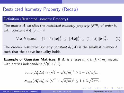
Restricted Isometry Property (Recap)

Definition (Restricted Isometry Property)

The matrix A satisfies the restricted isometry property (RIP) of order k,with constant δ ∈ [0, 1), if

∀ x k-sparse, (1− δ) ‖x‖22 ≤ ‖Ax‖22 ≤ (1 + δ) ‖x‖22 . (1)

The order-k restricted isometry constant δk(A) is the smallest number δsuch that the above inequality holds.

Example of Gaussian Matrices: If AI is a large m× k (k < m) matrixwith entries independent N (0, 1/m),

σmin(A∗I AI) ≈ (√

1−√k/m)2 ≥ 1− 2

√k/m,

σmax(A∗I AI) ≈ (√

1 +√k/m)2 ≤ 1 + 3

√k/m.


The Johnson-Lindenstrauss Lemma

Length Concentration of Gaussian Vectors

Lemma (Gaussian Vectors1)

Let g = [g1, . . . , gm]∗ ∈ Rm be an m-dimensional random vector whoseentries are iid N (0, 1/m). Then for any t ∈ [0, 1],

P[∣∣∣‖g‖22 − 1

∣∣∣ > t]≤ 2 exp

(− t

2m

8

). (2)

Proof (sketch): The moment generating function of a standard normalrandom variable is

E[eλx

2]= (1− 2λ)−1/2, λ < 1/2.

Then we have E[eλg

2i]

=(1− 2λ

m

)−1/2, λ < m

2 .

1This result can be obtained via the Cramer-Chernoff exponential moment method(see Appendix E) or the book: High-Dimensional Probability, Roman Vershynin, 2018.



Length Concentration of Gaussian Vectors

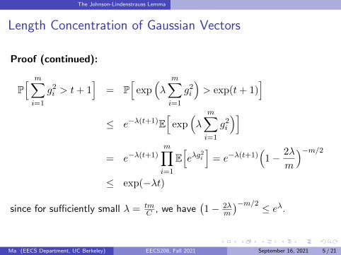
Proof (continued):

P[ m∑i=1

g2i > t+ 1

]= P

[exp

(λ

m∑i=1

g2i

)> exp(t+ 1)

]≤ e−λ(t+1)E

[exp

(λ

m∑i=1

g2i

)]= e−λ(t+1)

m∏i=1

E[eλg

2i

]= e−λ(t+1)

(1− 2λ

m

)−m/2≤ exp(−λt)

since for sufficiently small λ = tmC , we have

(1− 2λ

m

)−m/2 ≤ eλ.



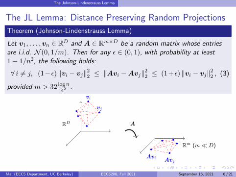
The JL Lemma: Distance Preserving Random Projections

Theorem (Johnson-Lindenstrauss Lemma)

Let v1, . . . ,vn ∈ RD and A ∈ Rm×D be a random matrix whose entriesare i.i.d. N (0, 1/m). Then for any ε ∈ (0, 1), with probability at least1− 1/n2, the following holds:

∀ i 6= j, (1−ε) ‖vi − vj‖22 ≤ ‖Avi −Avj‖22 ≤ (1+ε) ‖vi − vj‖22 , (3)

provided m > 32 lognε2

.

RD A

Rm (m D)

vi

vj

AvjAvi



The JL Lemma

Proof.

Finite cases: let gij = Avi−vj

‖vi−vj‖2for any i 6= j ∈ 1, . . . , n.

Tail bound: gij is distributed as an iid Gaussian vector, with entriesN (0, 1/m). Applying Lemma:

P[∣∣∣‖gij‖22 − 1

∣∣∣ > t]≤ 2 exp

(−t2m/8

). (4)

Union bound: Summing the probability of failure over all i 6= j, and thenplugging in t = ε and m ≥ 32 log n/ε2, we get

P[∃ (i, j) :

∣∣∣‖gij‖22 − 1∣∣∣ > t

]≤ n(n− 1)

2× 2 exp

(−t2m/8

)≤ n−2. (5)

Hence∣∣∣‖gij‖22 − 1

∣∣∣ ≤ ε with probability 1− n−2.



The JL Lemma: Generalization to `p Norms

Locality-Sensitive Hashing2: for p ∈ (0, 2], there exist the so-calledp-stable distributions such that a random matrix A drawn from a p-stabledistribution will preserve `p distance between vectors:

(1− ε) ‖vi − vj‖2p ≤ ‖Avi −Avj‖2p ≤ (1 + ε) ‖vi − vj‖2p . (6)

Example: For `1 norm, the corresponding distribution is the Cauchydistribution with density:

p(x) =1

π· 1

1 + x2.

2Locality-sensitive hashing scheme based on p-stable distributions, M. Datar, N.Immorlica, P. Indyk, and V. S. Mirrokni. ACM SCG 2004.



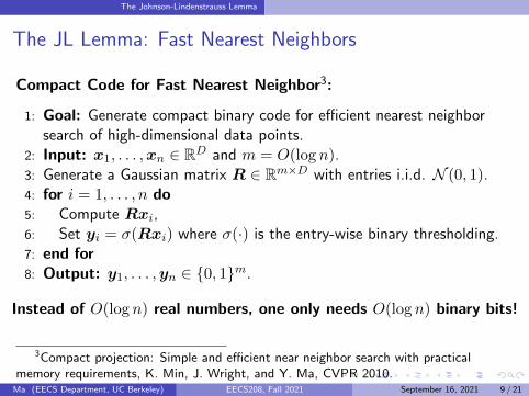
The JL Lemma: Fast Nearest Neighbors

Compact Code for Fast Nearest Neighbor3:

1: Goal: Generate compact binary code for efficient nearest neighborsearch of high-dimensional data points.

2: Input: x1, . . . ,xn ∈ RD and m = O(log n).3: Generate a Gaussian matrix R ∈ Rm×D with entries i.i.d. N (0, 1).4: for i = 1, . . . , n do5: Compute Rxi,6: Set yi = σ(Rxi) where σ(·) is the entry-wise binary thresholding.7: end for8: Output: y1, . . . ,yn ∈ 0, 1m.

Instead of O(log n) real numbers, one only needs O(log n) binary bits!

3Compact projection: Simple and efficient near neighbor search with practicalmemory requirements, K. Min, J. Wright, and Y. Ma, CVPR 2010.


RIP of Gaussian Matrices


Theorem (RIP of Gaussian Matrices)

There exists a numerical constant C > 0 such that if A ∈ Rm×n is arandom matrix with entries independent N

(0, 1

m

)random variables, with

high probability, δk(A) < δ, provided

m ≥ Ck log(n/k)/δ2. (7)

Implications: `1 minimization can successfully recover k-sparse solutionsxo from about

m ≥ Ck log(n/k) ∼ Ω(k)

random measurements.



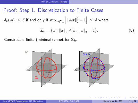
Proof: Step 1. Discretization to Finite Cases

δk(A) ≤ δ if and only if supx∈Σk

∣∣∣‖Ax‖22 − 1∣∣∣ ≤ δ where

Σk = x | ‖x‖0 ≤ k, ‖x‖2 = 1. (8)

Construct a finite (minimal) ε-net for Σk.



Proof: Step 1. Discretization to Finite CasesAn ε-net (or covering) N for a given set S if

∀x ∈ S, ∃ x ∈ N such that ‖x− x‖2 ≤ ε. (9)

A set M is ε-separated if every pair of distinct points x,x′ in M hasdistance at least ε:

‖x− x′‖2 ≥ ε. (10)

Fact: A maximal ε-separated subset M ⊂ S is a (minimal) ε-net of S.




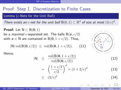
Lemma (ε-Nets for the Unit Ball)

There exists an ε-net for the unit ball B(0, 1) ⊂ Rd of size at most (3/ε)d.

Proof: Let N ⊂ B(0, 1)be a maximal ε-separated set. The balls B(x, ε/2)with x ∈ N are contained in B(0, 1 + ε/2). Thus,

|N| vol(B(0, ε/2)) ≤ vol(B(0, 1 + ε/2)). (11)

Hence,

|N| ≤ vol(B(0, 1 + ε/2))

vol(B(0, ε/2))(12)

=

(1 + ε/2

ε/2

)d= (1 + 2/ε)d (13)

≤ (3/ε)d (14)




Lemma (Discretization)

Suppose we have a set N ⊆ Σk with the following property: for all x ∈ Σk,there exists x ∈ N such that

• |supp(x) ∪ supp(x|) ≤ k

• ‖x− x‖2 ≤ ε.set

δN = maxx∈N

∣∣∣‖Ax‖22 − 1∣∣∣ . (15)

Then

δk(A) ≤ δN + 2ε

1− 2ε. (16)

Implications: RIP constant δ does not change much if we restrict ourcalculation to a finite ε-covering set N.




Lemma (ε-Nets for Σk)

There exists an ε-net N for Σk satisfying the two properties required inLemma 6, with ∣∣N∣∣ ≤ exp

(k log(3/ε) + k log(n/k) + k

). (17)

Proof.

Constructing an ε-Net for each ball in Σk and take the union. Using theStirling’s formula,4 we can estimate

∣∣N∣∣ ≤ (3/ε)k(n

k

)≤ (3/ε)k

(nek

)k. (18)

4Stirling’s formula gives the bounds for factorials:√2πk

(ke

)k ≤ k! ≤ e√k( ke

)k.



Proof: Steps 2 and 3Step 2: Tail Bound for Probability of Each Failure Case:For each x ∈ N, Ax is a random vector with entries independentN (0, 1/m). We have

P[∣∣∣‖Ax‖22 − 1

∣∣∣ > t]≤ 2 exp(−mt2/8). (19)

Step 3: Union Bound for Probability of All Failure Cases:Summing over all elements of N, we have

P [δN > t] ≤ 2∣∣N∣∣ exp

(−mt2/8

)(20)

≤ 2 exp(− mt2

8+ k log

(nk

)+ k(log

(3

ε

)+ k)

). (21)

On the complement of the event δN > t, we have

δk(A) ≤ 2ε+ t

1− 2ε. (22)

Setting ε = δ/8, t = δ/4, and ensuring that m ≥ Ck log(n/k)/δ2 forsufficiently large numerical constant C, we obtain the result.



RIP of Order k for Gaussian Matrices A ∈ Rm×n

From the above derivation, especially from equation (21), we see thata slight more tight bound for m is of the form

m ≥ 128k log(n/k)/δ2 + (log(24/δ) + 1)k/δ2 .= C1k log(n/k) + C2k.

For a small δ, the constants C1 and C2 can be rather large.

A much tighter bound (one of the best known) for m is given as5:

m ≥ 8k log(n/k) + 12k.

A precise (phase transition) expressionof m as function of k, n exists(Lecture Eight: Section 3.6 or Chapter 6).

5On sparse reconstruction from Fourier and Gaussian measurements, M. Rudelsonand R. Vershynin. Comm. on Pure and Applied Mathematics, 2008.


RIP of Non-Gaussian Matrices

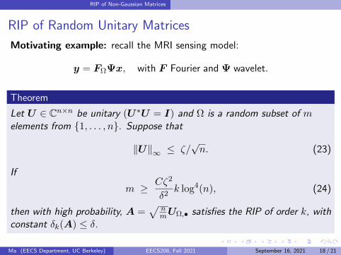
RIP of Random Unitary Matrices

Motivating example: recall the MRI sensing model:

y = FΩΨx, with F Fourier and Ψ wavelet.

Theorem

Let U ∈ Cn×n be unitary (U∗U = I) and Ω is a random subset of melements from 1, . . . , n. Suppose that

‖U‖∞ ≤ ζ/√n. (23)

If

m ≥ Cζ2

δ2k log4(n), (24)

then with high probability, A =√

nmUΩ,• satisfies the RIP of order k, with

constant δk(A) ≤ δ.



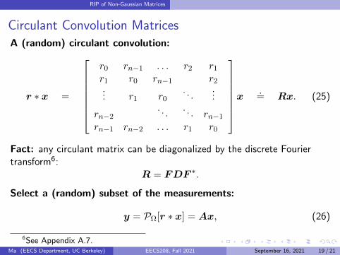
Circulant Convolution MatricesA (random) circulant convolution:

r ∗ x =

r0 rn−1 . . . r2 r1

r1 r0 rn−1 r2... r1 r0

. . ....

rn−2. . .

. . . rn−1

rn−1 rn−2 . . . r1 r0

x.= Rx. (25)

Fact: any circulant matrix can be diagonalized by the discrete Fouriertransform6:

R = FDF ∗.

Select a (random) subset of the measurements:

y = PΩ[r ∗ x] = Ax, (26)

6See Appendix A.7.Ma (EECS Department, UC Berkeley) EECS208, Fall 2021 September 16, 2021 19 / 21


RIP of Random Circulant Convolution Matrices

Let r be a random vector with independent zero-mean, subgaussianrandom variables of variance one.

Theorem

Let Ω ⊆ 1, . . . , n be any fixed subset of size |Ω| = m. Then if

m ≥ Ck log2(k) log2(n)

δ2, (27)

then with high probability, A has RIP of order k with δk(A) ≤ δ.

Approximate isometric property is the key to deep convolutionneural networks!7

7Deep Isometric Learning for Visual Recognition, H. Qi, C. You, X. Wang, Yi Ma,and J. Malik, ICML 2020.



Assignments

• Reading: Section 3.4 of Chapter 3.


computational principles for high-dim data analysis 3mm

Documents