Computational Modeling of Human Head Electromagnetics for Source Localization of Milliscale Brain Dynamics using GPUS

A. Salman1, S. Turovets1,2, V. Volkov3, A. Malony1, D. Tucker2, P. Luu2, D. Ozog1 1Neuroinformatics Center, University of Oregon 2Electrical Geodesics, Inc. 3Belarusian State University, Minsk, Belarus

Advances in human brain science have been closely linked with new developments in neuroimaging technology. Brain activity takes place at millisecond temporal and millimeter spatial scales through the reentrant, bidirectional interactions of functional neural networks distributed throughout the cortex and interconnected by a complex network of white matter fibers. Our research goal has been to create an anatomically-constrained, spatiotemporally-optimized neuroimaging (ACSON) methodology to improve the source localization of dense-array EEG (dEEG). Anatomical constraints include high-resolution three-dimensional segmentation of an individual's head tissues, identification of head tissue conductivities, alignment of source generator dipoles with the individual's cortical surface, and interconnection of cortical regions through the white matter tracts. Using these constraints, the ACSON constructs a full-physics computational model of an individual's head electromagnetics and uses is to map measured EEG scalp potentials to their cortical sources. The ACSON workflow (see diagram) poses several major computational challenges to be applied in practice. High-performance parallel implementations of the electromagnetic solvers using GPUs has enabled the creation of one of the first full-resolution, FDM construction of a real human head for source localization based on electromagnetics simulation.

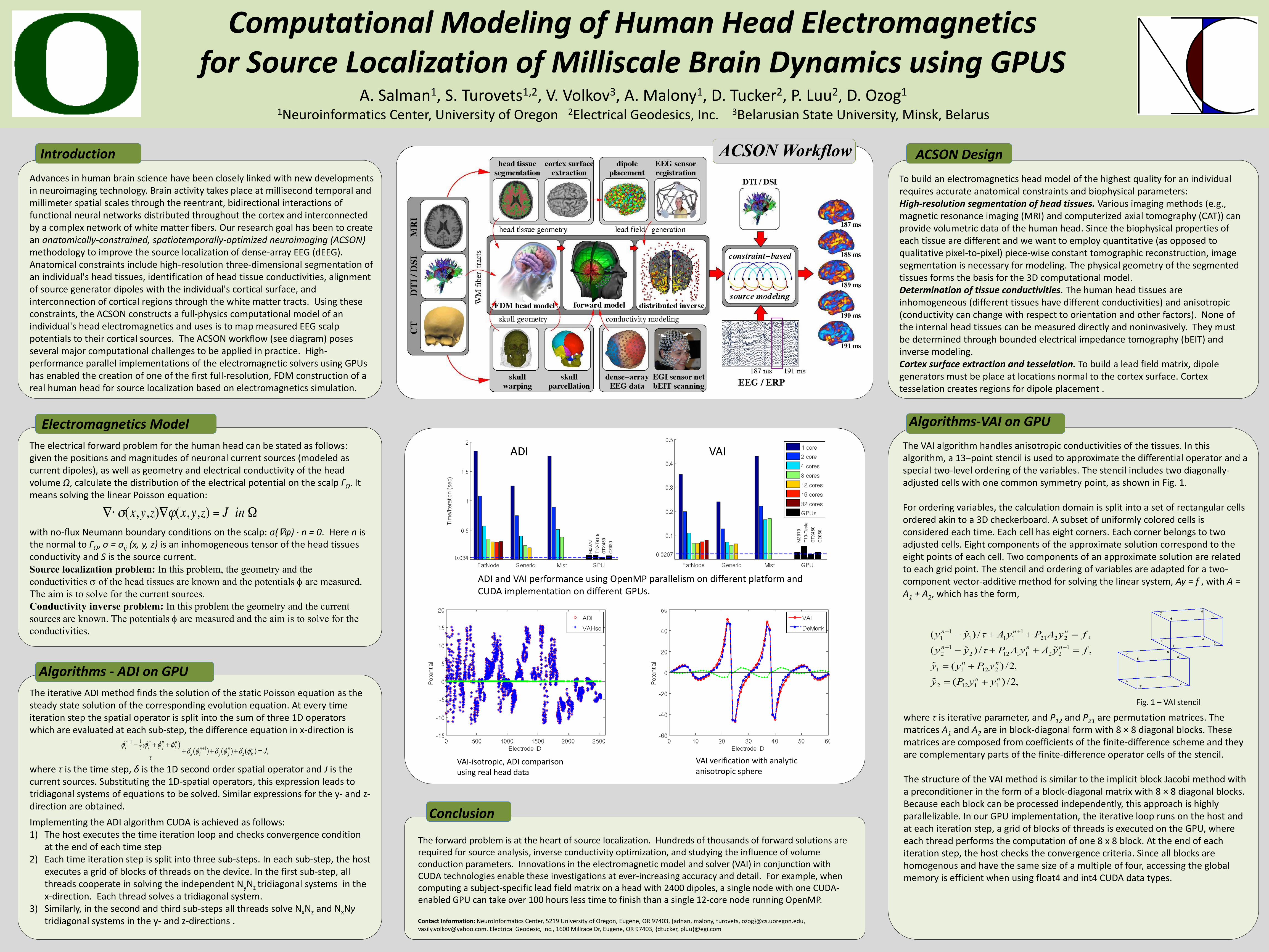
ACSON Design ACSON Workflow

To build an electromagnetics head model of the highest quality for an individual requires accurate anatomical constraints and biophysical parameters: High-resolution segmentation of head tissues. Various imaging methods (e.g., magnetic resonance imaging (MRI) and computerized axial tomography (CAT)) can provide volumetric data of the human head. Since the biophysical properties of each tissue are different and we want to employ quantitative (as opposed to qualitative pixel-to-pixel) piece-wise constant tomographic reconstruction, image segmentation is necessary for modeling. The physical geometry of the segmented tissues forms the basis for the 3D computational model. Determination of tissue conductivities. The human head tissues are inhomogeneous (different tissues have different conductivities) and anisotropic (conductivity can change with respect to orientation and other factors). None of the internal head tissues can be measured directly and noninvasively. They must be determined through bounded electrical impedance tomography (bEIT) and inverse modeling. Cortex surface extraction and tesselation. To build a lead field matrix, dipole generators must be place at locations normal to the cortex surface. Cortex tesselation creates regions for dipole placement .

The electrical forward problem for the human head can be stated as follows: given the positions and magnitudes of neuronal current sources (modeled as current dipoles), as well as geometry and electrical conductivity of the head volume Ω, calculate the distribution of the electrical potential on the scalp ΓΩ. It means solving the linear Poisson equation: with no-flux Neumann boundary conditions on the scalp: σ(∇φ) · n = 0. Here n is the normal to ΓΩ, σ = σij (x, y, z) is an inhomogeneous tensor of the head tissues conductivity and S is the source current. Source localization problem: In this problem, the geometry and the

conductivities of the head tissues are known and the potentials are measured.

The aim is to solve for the current sources.

Conductivity inverse problem: In this problem the geometry and the current

sources are known. The potentials are measured and the aim is to solve for the

conductivities.

Electromagnetics Model

The iterative ADI method finds the solution of the static Poisson equation as the steady state solution of the corresponding evolution equation. At every time iteration step the spatial operator is split into the sum of three 1D operators which are evaluated at each sub-step, the difference equation in x-direction is

 

fi

n +1 -1

3(fi

n + f j

n + fk

n )

t+dx (fi

n +1) +dy(f j

n ) +dz(fk

n ) = J,

where τ is the time step, δ is the 1D second order spatial operator and J is the current sources. Substituting the 1D-spatial operators, this expression leads to tridiagonal systems of equations to be solved. Similar expressions for the y- and z-direction are obtained.

Implementing the ADI algorithm CUDA is achieved as follows: 1) The host executes the time iteration loop and checks convergence condition

at the end of each time step 2) Each time iteration step is split into three sub-steps. In each sub-step, the host

executes a grid of blocks of threads on the device. In the first sub-step, all threads cooperate in solving the independent NyNz tridiagonal systems in the x-direction. Each thread solves a tridiagonal system.

3) Similarly, in the second and third sub-steps all threads solve NxNz and NxNy tridiagonal systems in the y- and z-directions .

The forward problem is at the heart of source localization. Hundreds of thousands of forward solutions are required for source analysis, inverse conductivity optimization, and studying the influence of volume conduction parameters. Innovations in the electromagnetic model and solver (VAI) in conjunction with CUDA technologies enable these investigations at ever-increasing accuracy and detail. For example, when computing a subject-specific lead field matrix on a head with 2400 dipoles, a single node with one CUDA-enabled GPU can take over 100 hours less time to finish than a single 12-core node running OpenMP. Contact Information: NeuroInformatics Center, 5219 University of Oregon, Eugene, OR 97403, {adnan, malony, turovets, ozog}@cs.uoregon.edu, vasily.volkov@yahoo.com. Electrical Geodesic, Inc., 1600 Millrace Dr, Eugene, OR 97403, {dtucker, pluu}@egi.com

Conclusion

Algorithms-VAI on GPU

The VAI algorithm handles anisotropic conductivities of the tissues. In this algorithm, a 13−point stencil is used to approximate the differential operator and a special two-level ordering of the variables. The stencil includes two diagonally-adjusted cells with one common symmetry point, as shown in Fig. 1. For ordering variables, the calculation domain is split into a set of rectangular cells ordered akin to a 3D checkerboard. A subset of uniformly colored cells is considered each time. Each cell has eight corners. Each corner belongs to two adjusted cells. Eight components of the approximate solution correspond to the eight points of each cell. Two components of an approximate solution are related to each grid point. The stencil and ordering of variables are adapted for a two-component vector-additive method for solving the linear system, Ay = f , with A = A1 + A2, which has the form,

 

(y1

n +1 - ˜ y 1) /t + A1y1

n +1 + P21A2y2

n = f ,

(y2

n +1 - ˜ y 2) /t + P12A1y1

n + A2˜ y 2

n +1 = f ,

˜ y 1 = (y1

n + P12y2

n ) /2,

˜ y 2 = (P12y1

n + y1

n ) /2,

where τ is iterative parameter, and P12 and P21 are permutation matrices. The matrices A1 and A2 are in block-diagonal form with 8 × 8 diagonal blocks. These matrices are composed from coefficients of the finite-difference scheme and they are complementary parts of the finite-difference operator cells of the stencil. The structure of the VAI method is similar to the implicit block Jacobi method with a preconditioner in the form of a block-diagonal matrix with 8 × 8 diagonal blocks. Because each block can be processed independently, this approach is highly parallelizable. In our GPU implementation, the iterative loop runs on the host and at each iteration step, a grid of blocks of threads is executed on the GPU, where each thread performs the computation of one 8 x 8 block. At the end of each iteration step, the host checks the convergence criteria. Since all blocks are homogenous and have the same size of a multiple of four, accessing the global memory is efficient when using float4 and int4 CUDA data types.

VA VA ADI and VAI performance using OpenMP parallelism on different platform and CUDA implementation on different GPUs.

VAI verification with analytic anisotropic sphere

VAI-isotropic, ADI comparison using real head data

Algorithms - ADI on GPU

Fig. 1 – VAI stencil

ADI VAI

Introduction