Computational Methods in Physics

Pawel Scharoch

February 25, 2014

Wroclaw University of Technology, Wyb. Wyspianskiego 27, 50-370 Wroclaw, Poland

1

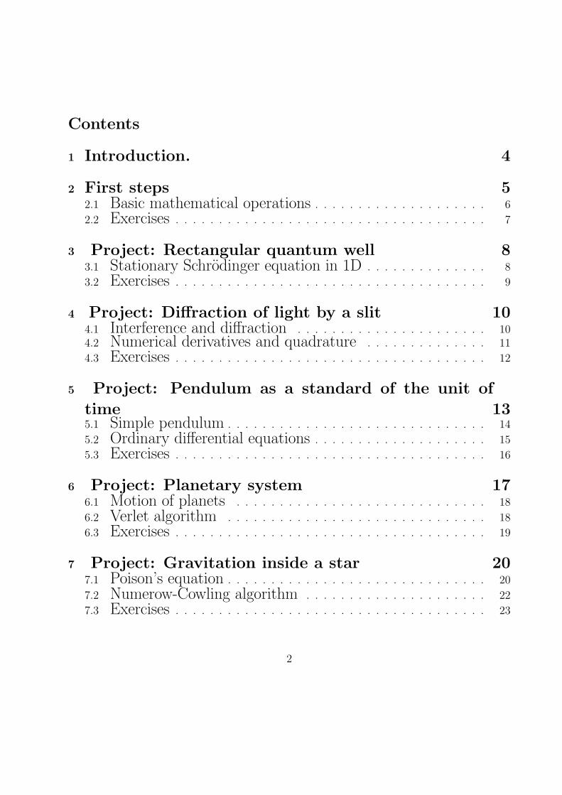
Contents

1 Introduction. 4

2 First steps 52.1 Basic mathematical operations . . . . . . . . . . . . . . . . . . . . 6

2.2 Exercises . . . . . . . . . . . . . . . . . . . . . . . . . . . . . . . . . . . . 7

3 Project: Rectangular quantum well 83.1 Stationary Schrodinger equation in 1D . . . . . . . . . . . . . . 8

3.2 Exercises . . . . . . . . . . . . . . . . . . . . . . . . . . . . . . . . . . . . 9

4 Project: Diffraction of light by a slit 104.1 Interference and diffraction . . . . . . . . . . . . . . . . . . . . . . 104.2 Numerical derivatives and quadrature . . . . . . . . . . . . . . 11

4.3 Exercises . . . . . . . . . . . . . . . . . . . . . . . . . . . . . . . . . . . . 12

5 Project: Pendulum as a standard of the unit of

time 135.1 Simple pendulum . . . . . . . . . . . . . . . . . . . . . . . . . . . . . . 14

5.2 Ordinary differential equations . . . . . . . . . . . . . . . . . . . . 15

5.3 Exercises . . . . . . . . . . . . . . . . . . . . . . . . . . . . . . . . . . . . 16

6 Project: Planetary system 176.1 Motion of planets . . . . . . . . . . . . . . . . . . . . . . . . . . . . . 18

6.2 Verlet algorithm . . . . . . . . . . . . . . . . . . . . . . . . . . . . . . 18

6.3 Exercises . . . . . . . . . . . . . . . . . . . . . . . . . . . . . . . . . . . . 19

7 Project: Gravitation inside a star 207.1 Poison’s equation . . . . . . . . . . . . . . . . . . . . . . . . . . . . . . 20

7.2 Numerow-Cowling algorithm . . . . . . . . . . . . . . . . . . . . . 22

7.3 Exercises . . . . . . . . . . . . . . . . . . . . . . . . . . . . . . . . . . . . 23

2

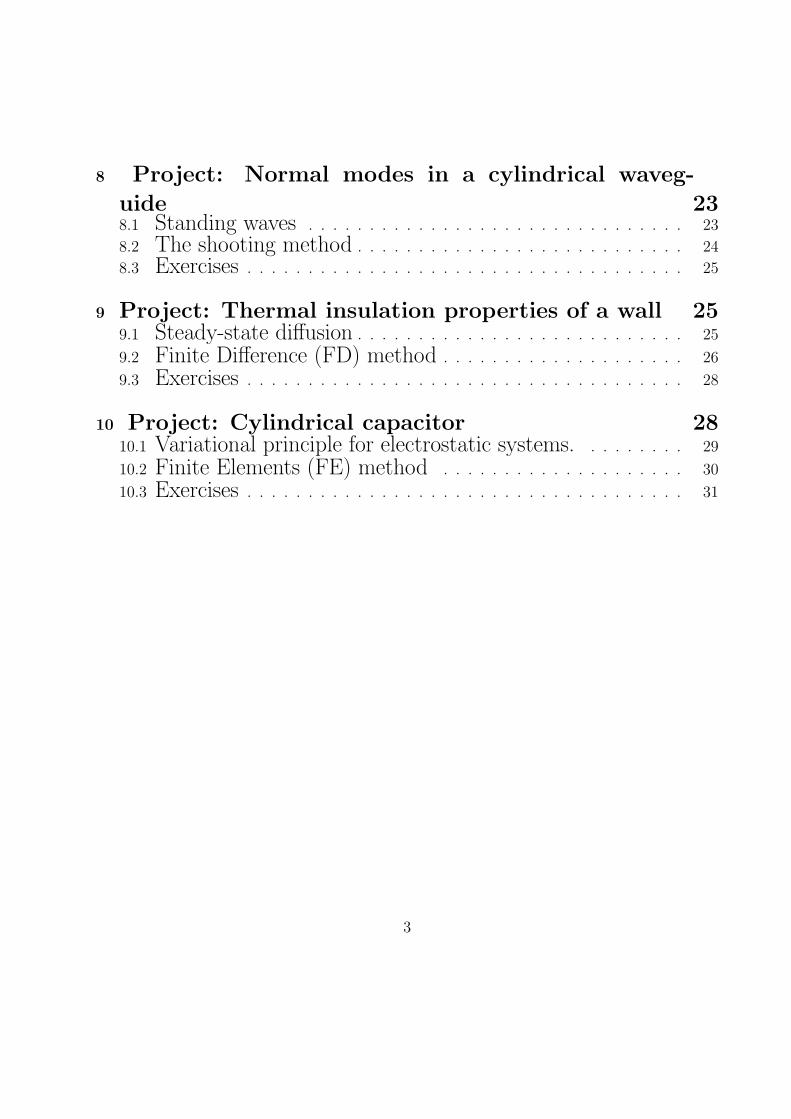
8 Project: Normal modes in a cylindrical waveg-

uide 238.1 Standing waves . . . . . . . . . . . . . . . . . . . . . . . . . . . . . . . 23

8.2 The shooting method . . . . . . . . . . . . . . . . . . . . . . . . . . . 24

8.3 Exercises . . . . . . . . . . . . . . . . . . . . . . . . . . . . . . . . . . . . 25

9 Project: Thermal insulation properties of a wall 259.1 Steady-state diffusion . . . . . . . . . . . . . . . . . . . . . . . . . . . 25

9.2 Finite Difference (FD) method . . . . . . . . . . . . . . . . . . . . 26

9.3 Exercises . . . . . . . . . . . . . . . . . . . . . . . . . . . . . . . . . . . . 28

10 Project: Cylindrical capacitor 2810.1 Variational principle for electrostatic systems. . . . . . . . . 29

10.2 Finite Elements (FE) method . . . . . . . . . . . . . . . . . . . . 30

10.3 Exercises . . . . . . . . . . . . . . . . . . . . . . . . . . . . . . . . . . . . 31

3

1 Introduction.

Numerical modeling is a powerful scientific tool. Its spectacular development could be ob-served over the last half century, as one of the consequences of advances in computer technol-ogy. Today, no field of science or engineering can be found were the computational methodswould not play one of crucial roles. The list of their advantages is long. New opportunitieshave emerged, like: the ability of ”predicting”, of investigating into properties unavailableexperimentally, obtaining quantitative data requiring huge amount of mathematical opera-tions or processing of huge amount of data. Those new opportunities are accompanied bythe relative easiness of application and low costs. Nowadays, the computational research,owing to the mentioned above features, constitutes an independent scientific tool (besidestraditional experiment and theory), which on the one hand, is an extension of mathematicalmodeling and could not exist without it, but on the other hand, creates its own methodologyand often resembles experimental rather than theoretical work (computational experiments).

In view of the above remarks, it is obvious that various aspects of numerical modelingshould become an important element of academic education, particularly at science and en-gineering faculties. In fact, such an element of education has been offered for many years byuniversities all over the world, even in the form of a separate specialization (like e.g. Ap-plied Computer Science), which concentrates on various aspects of applications of computersin science and technology, and on numerical modeling in particular. This course (Compu-tational Methods in Physics) is a response to this need. This is a ”Numerical Modeling”course, whose philosophy is similar to that proposed by S.Koonin [1], but has been modified,adjusted to more elementary level, and supplemented with additional issues and examples.The idea of the course is that it is purpose-oriented, i.e. a numerical method is introducedas a tool to solve a particular physical problem, so that a participant has the feeling ofapplicability of the method he or she learns. An additional advantage is learning physics,since the computer programs on which the participants work allow them to investigate intoproperties of chosen systems. The course is constructed as a series of Projects, which arehere to provide a good reason and motivation for learning numerical methods. Thus, everySubject Unit (Project) begins with presenting the physics problem, discussing it and identi-fying the mathematical tools needed. Then, an appropriate numerical method is introduced,the algorithm is developed and a respective computer code is shown and discussed.

The methods taught cover basic mathematical operations (finding roots and minima),derivatives and integrals, ordinary and partial differential equations (initial value problem(IVP), boundary value problem (BVP), eigenvalue problem (EVP)). Most methods are basedon discretisations of variables. The physical systems are chosen so that their simulationcould be relatively simple (the programming, tests and experiments could be done during1-2 sessions), thus the methods specific for the partial differential equations are illustrated

4

by 1D systems. The students are given preliminary versions of the codes. On the level ofprogramming, the basic elements of FORTRAN programming language are used, since themain objective of the course is to teach numerical methods, not a particular programminglanguage, thus the algorithms can be easily transferred to other platforms (MATLAB, C++,Delfi, Python, etc.). During computer laboratory sessions students have an opportunityto test and modify the codes, and finally perform some experiments which resemble thereal ones, but offer much more freedom of setting the conditions and therefore open largespace for creativity and learning physics. For the freeware FORTRAN language the Forceenvironment is used and for the graphical representation of data the freeware GNUPLOT isrecommended. Using the freeware software allows students to work on the lab projects alsoat home. Getting familiar with this software can be very useful for them also in the future.

This material is organized in the following way. Each chapter begins with a brief sum-mary of its content followed by the theoretical background section, containing a summaryof the theoretical foundation of the considered problem, and the numerical procedures sec-tion introducing the respective numerical algorithms and presenting the final formulae ofthe schemes to be applied in the programs. No derivations in those chapters are presented,only some hints, how a particular formula can be derived, are given, thus further reading isstrongly recommended of any standard physics textbook (at academic level) as well as onnumerical methods, e.g. [1, 2, 3] (at the beginning of each section the preliminary readingnote points at the physics part which should be recalled or learned in advance). It is alsorecommended that a student derives by himself every formula presented in this book (thisshould be treated as an obligatory exercise for each session which has not been explicitlymentioned in the text). Finally a section Exercises follows in which students will find a setof exercises to be done with the particular computer code. The computer codes have beenprepared and tested in advance and are provided as an integral part of this book. The codeshave not been optimized so that the implementation of the algorithms is clearer. Studentsare free to modify the codes when doing the exercises or to implement their own ideas.

2 First steps

Prerequisities: basic computer knowledge (Windows or Linux operating system).

This is the first computer lab session during which students learn (or recall) basic el-ements of FORTRAN programming language (program structure, declaration of variables,input/output declarations and instructions), the Force environment for FORTRAN (editionand compilation of the program, debugging), and basic instructions of GNUPLOT graphi-

5

cal environment (plot, splot, set xrange). Basic numerical procedures are also introduced:tabulating 1D and 2D functions, finding roots and finding a minimum in 1D.

2.1 Basic mathematical operations

Content: tabulating a function 1D i 2D, finding roots (Bisection, Secant, Newton-Raphsonmethod), finding a minimum in 1D (Golden Section Search for a minimum in 1D, methodbased on the parabolic interpolation, Simplex method in 1D).

Finding roots, Bisection methodWe start from the point where we are sure that the root of a function f(x) is somewhere

within the interval (xl, xr). To reduce the interval we cut it half and find the point in themiddle xm. We get then two new intervals and we have to identify the one within which thefunction crosses zero. This can be easily done by checking the condition e.g. f(xl)·f(xm) < 0(the function changes its sign). We denote the ends of the new interval again by (xl, xr) andrepeat the procedure. After n steps the lengths of the domain segment containing zeroreduces by factor 2n and when it is less then assumed accuracy ϵ the whole procedure stops.

The bisection method is very safe but not most efficient. The popular alternatives areSecant and Newton-Raphson methods. The Newton-Raphson method is useful when togetherwith the function f(x) also its analytical derivative is known. Using the derivative weconstruct a linear function being tangent to f(x) at the starting point. Then we approximatethe root of f(x) by the zero of the linear function. This root is treated as the new startingpoint and the construction repeats. In many cases the procedure is very quickly convergentbut this is not always the case, thus should be applied with a caution. The secant method issimilar to the Newton-Raphson one except the derivative of a function is found numerically,using e.g. a 3-point scheme (see Chapter 4.2)

Finding minimum in 1D, Golden Section SearchTo identify the domain interval containing a minimum we need a checking point xc

within the interval (xl, xr). We can be sure that the minimum is present in the intervalif f(xc) < f(xl) and f(xc) < f(xr). In constructing the algorithm one should focus on aproper choice of the new, fourth checking point xn. By introducing the fourth point in theinterval (xl, xr) we obtain two overlapping regions each defined by 3 points. We can thenidentify the one containing the minimum (the condition above). To assure the optimumconvergence the two regions should have the smallest possible and the same length (at each

6

step). This can be achieved if at each step the fourth point splits the longer of the twosegments (xl, xc) and (xc, xr) in golden section proportion, i.e. hl/(hl + hs) = hs/hl (hl -longer segment, hs - shorter segment) so that the two new intervals containing 3 point haveequal length. By substituting x = hs/hl into the above golden section condition we get theequation x2+x− 1 = 0 whose one of solutions (

√5− 1)/2 ≈ 0.62 is the golden section ratio.

Thus, after n steps the length of starting interval is reduced by factor ≈ 0.62n, which is alittle bit slower then in bisection algorithm.

The Golden Section Search is always convergent but not necessarily most effective. Usu-ally, very effective is the algorithm in which the forth checking point is found as the minimumof the second order polynomial interpolation of the function between 3 initial points. Theeffectiveness is connected with the fact that many functions near minimum have leadingsecond order term in the power series expansion.

The Simplex method is the most simple search of the minimum which uses a ”test win-dow” rather than 3 points. Starting from certain point the domain is scanned in the directionwhere function decreases (let us say to the right) by moving window (xl, xr) of certain lengthh = xr − xl. The minimum is found if the function begins to increase, i.e. f(xl) < f(xr).At this point the window length is cut half and the search continues from the xl where theincrease has been noticed. The procedure stops if h < ϵ, ϵ - the assumed accuracy.

If the analytical form of the first derivative is known then the minimum can be foundby finding a root of the derivative. The derivative can be also approximated by a numericalformula, this leads to more general form of the described above secant scheme.

2.2 Exercises

1. Compile and run the program FTABLE.2. Visualize chosen 1D function (set your own function) with the use of the program GNU-PLOT (plot command).3. Modify the program FTABLE so that it could tabulate a 2D function.4. Visualize chosen 2D function (set your own function) with the use of the program GNU-PLOT.5. Fit a function to an arbitrary set of data using GNUPLOT.6. Compile and run the program BISEC.7. Test the program by finding the roots of a chosen 2nd order polynomial and comparingthe results with the analytical solutions.8. Find the value of the number π as a zero of sinus function. What precision can youachieve, explain why ?9.(Advanced) Write the program 1DMINIMUM that finds the minimum of a 1D function

7

with one of algorithms discussed on the lecture (golden section, parabolas or 1D simplex).Test the program by finding the minimum of a chosen 2nd order polynomial and comparingthe results with the analytical solution. Find the value of the number π as a minimumposition of cosine function. What precision can you achieve, explain why ?

3 Project: Rectangular quantum well

Preliminary reading: stationary Schrodinger equation, rectangular quantum well as thesimplest model of a low dimensional or high symmetry quantum system.

In this project the participants use the finding roots procedure to solve the eigenvalueproblem of a rectangular quantum well (program QWELL). The program is then appliedto fit the simple quantum well results to a real system (hydrogen atom) by trial and errormethod.

3.1 Stationary Schrodinger equation in 1D

Content: eigenvalue problem for a rectangular quantum well and a method of its numericalsolution.

Stationary Schrodinger equation for a rectangular quantum well:[− ~2

2m

d2

dx2+ V (x)

]ψ(x) = εψ(x) (1)

where:

V (x) =

{−Vo if −a/2 ≤ x ≤ a/20 if x < −a/2 or x > a/2

In Hartree atomic units: ~ = me = e = 1:[ d2dx2

+ k2(x)]ψ(x) = 0 (2)

where k2(x) = 2(ε− V (x)).Solutions:

ψ(x) =

A cos(kx) for −a/2 ≤ x ≤ a/2 (even)A sin(kx) for −a/2 ≤ x ≤ a/2 (odd)B exp(∓kx) for x < −a/2 or x > a/2

(3)

8

The condition for the eigenvalue is that the two solutions (inside and outside the regionof the well) must join smoothly, i.e. their values and the values of their first derivatives mustbe equal e.g. at a/2 (because of symmetry it is sufficient to consider only one border). Thus,we have:

for even solutions: {±A cos(ka/2) = ±B exp(−κa/2)∓Ak sin(ka/2) = ∓Bκ exp(−κa/2)

and for odd solutions: {±A sin(ka/2) = ±B exp(−κa/2)±Ak cos(ka/2) = ∓Bκ exp(−κa/2)

where k =√

2(ε+ Vo) and κ =√−2ε

Dividing the first equation by the second one in the above systems we obtain two condi-tions, for even and odd solution:{

Feven(ε) = sin(ka/2)− κ/k · cos(ka/2) = 0 (even)Fodd(ε) = sin(ka/2) + k/κ · cos(ka/2) = 0 (odd)

(4)

The eigenvalues ε are found by solving the above equations.

3.2 Exercises

1. Compile and run the program QWELL.2. Tabulate functions Feven(ε) and Fodd(ε) (they are the functions, corresponding to evenand odd solutions respectively, whose zeros are energies of quantum levels)3. Visualize (in one figure) the functions Feven(ε) i Fodd(ε).4. Repeat the calculation and visualization of Feven(ε) i Fodd(ε) for different values of thewell parameters (a and V0).5. Square finite quantum well as a model of hydrogen.

a. draw a graph of an energy level as a function of the principal quantum number (n)for the hydrogen atom (in atomic units those energies a given by the formula 1/(2n2)).

b. try to fit the first two energy levels to the hydrogen ones through variation of theparameters a and V o, by trial and error method (hint: in the beginning set the valuesa = 2Bohr and Vo = 100Hartree).

9

4 Project: Diffraction of light by a slit

Preliminary reading: interference and diffraction phenomena.

By working on this project, the participants learn the numerical differentiation andquadrature procedures. In particular, the important issue of convergence with respect tothe grid parameter is discussed. The numerical quadrature procedure is used to constructa program (DIFFRACTION) simulating the diffraction of a scalar wave by a single infiniteslit and a system of parallel infinite slits. The program then serves for studying the physicsof the system.

4.1 Interference and diffraction

Content: interference and diffraction phenomena, the complex amplitude concept, discreteand continuous sources, diffraction integral, single infinite slit diffraction, diffraction grating.

The diffraction integral represents a superposition of complex amplitudes of waves emittedby elementary sources forming the whole continuous source (Huygens principle):

D =

∫Source

Ao(s)

rexp (−ikr + ϕ(s))ds (5)

where Ao(s) - amplitude at the elementary source, ϕ(s) - initial phase (at the elementarysource), k = 2π/λ - wave number, r - a distance from the elementary source to the observationpoint, (Ao(s)/r) exp (−ikr + ϕ(s)) - complex amplitude.

The intensity (forming the diffraction pattern) is given by:

I = |D|2 = Re(D)2 + Im(D)2 (6)

In the case of an infinite slit of width a the problem becomes 2-dimensional, in the sensethat no quantity varies in the direction parallel to the slit, so only two remaining directionsare of interest. Assuming that initial amplitude and phase (Ao, ϕ) are constant along the slitthe diffraction integral on the screen placed at the distance d takes the form:

D =

a/2∫−a/2

A(r) exp (−ikr)dx (7)

10

where r =√(y − x)2 + d2, A(r) = Ao/

√r (for a cylindrical wave emitted by an elemen-

tary line source), Ao - the amplitude at the source, x is the coordinate of the elementarysource and y - the coordinate of the observation point on the screen.

4.2 Numerical derivatives and quadrature

Content: various multipoint derivative and quadrature schemes based on the local interpo-lation of a function by a power series.

DerivativesSuppose we want to calculate numerically derivatives of various orders of a function f(x),

at certain point x. We start from power series expansions:f(x± h) = f(x)± f ′(x)h+ 1

2f ′′(x)h2 ± 1

6f ′′′(x)h3 + ...

f(x± 2h) = f(x)± f ′(x)2h+ 12f ′′(x)(2h)2 ± 1

6f ′′′(x)(2h)3 + ...)

...(8)

where h is a small grid parameter. The above power series expansions, when cut atcertain order, form a system of linear equations whose unknowns are subsequent derivatives.For example, if only the terms up to second order are preserved we get:{

f(x+ h) = f(x) + f ′(x)h+ 12f ′′(x)h2 +O(h3)

f(x− h) = f(x)− f ′(x)h+ 12f ′′(x)h2 +O(h3)

(9)

The symbol O(h3) means that the leading term in the rest of the series is on the orderof h3.

By subtracting or adding the equations (9) we easily derive the 3-point schemes for thefirst and the second derivative, respectively:

f ′(x) =f(x+ h)− f(x− h)

2h+O(h2) (10)

f ′′(x) =f(x+ h) + f(x− h)− 2f(x)

h2+O(h2) (11)

Note that the uncertainty of the second derivative is of the order of h2, this is becausethe leading terms of the third order in the two expansions cancel out. The above formulaeare called 3-point schemes because the local interpolation of the function based on 3 points(parabolic) is used. The formulae give exact values of derivatives for quadratic functions. It

11

is also interesting to note that the first derivative formula uses only 2 points, in spite of thefact that this is a 3-point scheme.

Using the above procedure it is easy to derive schemes based on a larger number ofpoints (higher order polynomial interpolations) as well as derivatives of a higher order. It isalso easy to incorporate a nonuniform grid (h is different at each step), although then theformulae become more complicated.

QuadratureThe schemes presented here are based on the assumption that the function f(x) which

we want to integrate is tabulated, i.e. its values are known at some points of the domainuniformly distributed along the integration interval. The grid parameter h is the distancebetween subsequent values of the argument in the grid: h = xi+1 − xi. The idea behindthe construction of the schemes is simple. Once we can calculate numerically the derivativesof any order at the points of the argument grid, the function can be interpolated by apolynomial of any order along certain local interval. Thus, it can also be locally integratedalong the same local interval. The quadrature along the whole interval of interest is obtainedby summing up the values of local integrals.

Very popular Simpson algorithm is based on the given above 3-point schemes for the firstand the second derivatives (and local quadratic interpolation of the function):

D =

h∫−h

f(x)dx =h

3(f(x+ h) + 4f(x) + f(x− h)) +O(h5) (12)

Note that the uncertainty of the quadrature is very low (on the order of h5). Could youexplain why?

It should be pointed out that the schemes of higher orders do not always lead to betterperformance of computer programs since they usually need more evaluations of the function(at a larger number of points). The same goal (better accuracy) can be achieved by reducingthe grid parameter h in the schemes of lower order. This can be easily done with moderncomputers and this is perhaps the reason why in the computational practice the 3-pointschemes are most popular.

4.3 Exercises

Numerical procedures1. Derive the 3-point and the 5-point finite difference formulae for the 1st and the 2ndderivatives of a function.2. Compile and run the program DERIV.

12

3. (Testing the program) Substitute your own function in the segment FUNC and calculateits derivatives. Compare the results with analytical values.4. Check the convergence of the 1st and the 2nd derivative with respect to the grid parameterh (draw derivatives as functions of −log10(h). Do the tests for a single and double precisionof real numbers. Discuss the results.5. Construct the function segments fp5 and fpp5 (the 1st and the 2nd derivative withe useof the 5-point scheme) and repeat the exercise 4. Compare the convergence of 3-point andthe 5-point schemes.6. Substitute a 2nd and a 5th order polynomial in the segment FUNC and test the convergencewith respect to h. Discuss of the results.7. Read, compile and run the program QUADRAT.8. Test the program by integrating a function whose analytical quadrature is known.9. Check the convergence of the Simpson algorithm with respect to the grid parameter h.How does it compare with the derivative convergence (discuss) ?10. Evaluate the number π from the length of an arc with use of the SIMPSON program.

Diffraction1. Read, compile and run the program DIFFRACTION.2. Test the program by comparing the first minimum position with the analytical value(sin(θ) = a/λ)3. Evaluate of diffraction patterns for different sets of input parameters and draw respectivegraphs (near and far field, narrow and wide slit etc.)4. Modify the program so that it could calculate the diffraction pattern produced by asystem of parallel slits (hint: use the loop to simulate a big number of slits, i.e. a diffractiongrating).5. Use the modified program to simulate a diffraction grating and draw graphs of diffractionpatterns for different grating parameters (the width and the separation of slits). Discuss theresults.6. (Advanced) Consider various initial phase distributions Φ(s) across a single slit (or atslits in diffraction grating). How do they affect the diffraction pattern ?6. (Advanced) Consider the case of diffraction due to circular aperture.

5 Project: Pendulum as a standard of the unit of time

Preliminary reading: Newton’s lows of motion, harmonic and anharmonic oscillators,driven oscillations, concept of a phase space.

13

This project is devoted to the Initial Value Problem for the ordinary differential equations.Participants learn various multipoint recursion schemes, apply them to some examples ofequations whose analytical solutions are known, check the convergence with respect to thegrid parameter and compare the quality of the schemes. Finally a chosen scheme is applied tostudy the properties of the compound pendulum, in particular the dependence of the periodof oscillation on energy. The results may serve to discuss the applicability of the pendulumas a standard of the unit of time.

5.1 Simple pendulum

Content: pendulum equation, initial conditions, scaling the equation, the case of smalloscillations (isochronism), the period in the whole range of energies, decomposition of the2nd order equation into a system of two 1st order equations, phase space.

Simple pendulum (point massm suspended from a massless, stiff rod of length l) equationof motion:

d2θ

dt2= −g

lsin(θ) (13)

θ is the swing angle, g - free fall acceleration.For small swing angles θ sin(θ) ≈ θ and the oscillation is harmonic:

d2θ

dt2= −g

lθ (14)

θ(t) = θosin(ωt) (15)

where θo - swing angle amplitude, ω = 2π/T =√g/l.

For small swing angles the period of oscillation T does not depend on the amplitude. Thisphenomenon (isochronism) allows us to use a pendulum as the standard of the unit of timein pendulum clocks (the first one constructed in 1656 by Christiaan Huygens). However,for bigger swing angles the period begins to change and to find it, it is necessary to solvenumerically the differential equation (13) for given inial values of angle and its first derivative(initial value problem).

A convenient way of setting the state of the pendulum is to use its total energy E =mgl(1−cos(θ))+ml2ω2/2 expressed in units of the maximum potential energy (with respectto the lowest position), i.e. ϵ = E/2mgl. Then we expect the period to be constant for

14

ϵ ≪ 1, to tend to infinity for ϵ approaching 1, and to behave like 1/√ϵ for ϵ ≫ 1 (explain

why?).

5.2 Ordinary differential equations

Content: Euler, Adams-Bashforth and Runge-Kutta schemes, the implicit and ’predictor-corrector’ algorithms.

The system of first order, linear, nonuniform differential equations:{dyidx

= f(y1, ..., yN , x) (16)

where x - independent variable, {y1, ..., yN} - dependent variables (functions of x).The linear differential equations of higher order can be decomposed into the system (16)

by defining auxiliary functions being derivatives of the function y(x).Developing the numerical methods for a single equation:

dy

dx= f(y, x) (17)

suffices, since the methods can be easily adopted to the system (16).A regular mesh (grid) of points {x0, x1, ..., xN}, in the interval (x0, xN) is introduced.

The distance between neighboring points: h = (xi+1 − xi), also h = (xN − x0)/N , is calledthe grid parameter h. We seek a recursion formula of the form:

yn+1 = F (yn, yn−1, yn−2, ...) (18)

which would allow to develop the function y(x), beginning from the initial point y0(x0).A starting formula is an exact integral of the equation (17) over the interval (xn, xn+1):

yn+1 = yn +

xn+1∫xn

f(x, y)dx (19)

In general the explicit form of f(x, y) is not known since the y(x) is not known (it is to befound). However, values of y(x) at previous points of mesh yn, yn−1, yn−2, ... are known andthey can be used to extrapolate y(x) over the interval (xn, xn+1). Depending on the numberof points used in the extrapolation we get so called explicit schemes of various orders. Forexample the most simple Euler’s formula (based on the extrapolation by a step function)reads:

15

yn+1 = yn + fnh+O(h2) (20)

where fn = F (xn, yn). The leading term of the local deviation from the exact solutionif on the order of h2 (explain why?). It should be noted that after N steps the uncertainty(global) will be one order lower because h ≃ 1/N , thus h2 ·N = h2/h = h.

The three step Adams-Bashforth scheme, based on the parabolic extrapolation has theform:

yn+1 = yn +h

12(5fn−2 − 16fn−1 + 23fn) +O(h4) (21)

The Runge-Kutta methods are based on more complicated mathematical idea which willnot be discussed here, although the integral (19) is still used as the starting point (forreference see e.g. [1, 2, 3]). They are regarded as the best integration schemes, whose greatadvantage is the fact that only one, already known, point xn, yn (e.g. the initial condition)is needed to perform an integration step, whereas the multipoint recursion schemes cannotbe started from a single initial condition. As an example, the 4th order Runge-Kutta schemehas the form:

k1 = hf(xn, yn)k2 = hf(xn + 1/2h, yn + 1/2k1)k3 = hf(xn + 1/2h, yn + 1/2k2)k4 = hf(xn + h, yn + k3)yn+1 = yn +

16(k1 + 2k2 + 2k3 + k4) +O(h6)

(22)

The unknown function y(x) appearing in the integrand (19) can be also interpolated bya polynomial of any order. In this case the unknown value yn+1 appears also on the righthand side of the formula and has to be evaluated by solving the equation. This strategyleads to a group of implicit schemes. They are most often used in the predictor-correctormethods in which a predicted value of yn+1 found from one of explicit is then corrected bythe implicit scheme of higher order.

5.3 Exercises

Numerical procedures1. Read, compile and run the program IVP.2. Evaluate the function being a solution to the differential equation dy/dx = −y withthe use of three schemes: Euler, 3rd order Adams-Bashforth and 5th order Runge-Kutta, atdifferent initial values, visualize the results.

16

3. Modify the code so that it is possible to check the convergence of solutions with respectto the grid parameter h. Classify different schemes with respect to convergence.4. Read, compile and run the program IVP2D.5. Evaluate the function being a solution to the differential equation d2y/dx2 = −k · y (theharmonic oscillator) with the use of a chosen scheme. Add in the code a line calculating thetotal energy of the oscillator and output the result. Find the range of the grid parameter atwhich the energy is conserved.7. (Advanced) Modify the code IVP2D code so that it could solve the equation d2y/dx2 +k · y−β ·dy/dx = Asin(ω ·x) (driven osillator); visualize and discuss the results for differentparameters (damping, elastic constant, frequency of driving force).8. (Advanced) Consider the case of coupled pendulums, described by the system of equations:

d2y1/dx2 = −k1 · y1 + γ · y2

d2y2/dx2 = −k2 · y2 + γ · y1

(23)

where γ is a coupling constant. Study the behavior of the system as dependent on itsphysical parameters.

Compound pendulum1. Read, compile and run the program PENDULUM.2.Test the program by comparing the results for small oscillations with the analytical solu-tion.3. Investigate into the dynamics of the physical pendulum for different total energies (the en-ergy is expressed in units of the maximum potential energy). Check the asymptotic behaviorof frequency or period (for low, system characteristic and high energy)4. Evaluate the function (T (E)− To)/To, where To is the small oscillation period.

6 Project: Planetary system

Preliminary reading: Newton’s law of universal gravitation, Newton’s laws of motion.

The molecular dynamics (MD) is one of most important kinds of simulation in physics.It is just solving the Newtonian equations of motion for a system of many particles. Therigorous analytical solution exists only for two-particle systems (and three-particle in specialcases), thus the computer simulation seems to provide the only possibility of studying suchsystems theoretically. The MD simulation is very popular in studying the dynamics and

17

thermodynamics of polyatomic systems but they are also used on a cosmic scale (motionof planets, stars, galaxies). All we need to know to construct the MD code is the law ofinteraction between the particles and Newton’s (or perhaps relativistic) equations of motion.In this project a simple 2-dimensional planetary system will be considered with two planetsand a fixed star as the source of the central force. Newton’s law of universal gravitation isused as the interaction law between planets and between planets and the star. The Verletalgorithm (most often used in MD simulation) for solving the initial value problem will beapplied.

6.1 Motion of planets

Content: equations of motion of planets, energy and angular momentum conservation.

The forces acting on planets due to the Star fixed in the origin of a reference system andto the other planet moving in the same plane:

F1 = −Gm1M

r21r1 −G

m1m2

r212r12

F2 = −Gm2M

r22r2 −G

m2m1

r221r21 (24)

where rij = rj − ri, and r = r/r is a unit vector associated with r.The Newton equations of motion for the two planets:

dp1/dt = F1

dr1/dt = p1/m1

dp2/dt = F2

dr2/dt = p2/m2

(25)

6.2 Verlet algorithm

Content: Verlet algorithm.The Verlet algorithm is a simple scheme developed for solving Newton’s equations of

motion for a system of particles (Molecular Dynamics), and is most often used in MD sim-ulations. Here, the idea of the algorithm is presented on the example of 1D motion, but itcan be easily generalized to the many dimensional case of a system of particles.

Newton’s equation of motion of a point mass m in 1D:

18

d2x

dt2= F/m (26)

where F - force acting on a particle of mass m, x - coordinate of the particle on the Xaxis.

To study the trajectory in phase space also the velocity v = dx/dt is needed.We use 3-point numerical formulae (10,11) to express position and velocity, which, when

rearranged lead to the following recursion schemes (Verlet’s algorithm):

xn+1 = 2xn − xn−1 + τ 2F/m+O(τ 4)vn = (xn+1 − xx−1)/(2τ) +O(τ 3)

(27)

where τ is the time step.It should be noted that as initial conditions usually position and velocity (or momentum)

are given (xo, vo), thus, there is certain difficulty in starting the recursion scheme since itneeds 2 initial points. The difficulty can be overcome e.g. by assuming that over the firsttime step the system performs the uniformly accelerated motion:

x1 = xo + voτ + (F/m)τ 2/2 +O(τ 3) (28)

which, however, is less accurate by 1 order of magnitude of τ and thus should be appliedwith caution. Alternatively, more accurate schemes (e.g. Runge-Kutta) over the first timestep can be used.

6.3 Exercises

1. Read, compile and run the program PLANETS.2. (Testing the program) Modify the code so that one of the planets is fixed far aside and itsmass is very low. Test the program on the example of motion of a single planet. Check theenergy and the momentum conservation. Find the maximum time-step for which the energyand the angular momentum are conserved. Compare the results with an analytical solutionfor a circular orbit.3. Try to find elliptic, parabolic and hyperbolic trajectories for a single planet (is it possibledistinguish between the parabolic and the hyperbolic ones in the computer simulation ?)(hint: use the total energy)4. By changing the mass of the fixed planet and its position observe its effect on thetrajectory of the second planet (the perturbation). Check the energy and the momentumconservation (should those quantities be both conserved ?). Can you observe a phenomenonof deterministic chaos ?

19

5. Include the motion of the second planet. Observe the dynamics of the system for differentinitial conditions. Check the energy and the angular momentum conservation.6. (Advanced) By introducing proper numerical values of the parameters observe the effectof the presence of Venus (or Mars) on the trajectory of the Earth (hint: keep the position ofVenus (Mars) fixed). Note that the period of motion of the Earth is about 365 days, whatis the time-step then ?7. (Advanced) Check Keppler’s laws of planetary motion.8. (Advanced) Propose an algorithm in which the time step would dynamically change tominimize the CPU time but preserving assumed accuracy of calculations.

7 Project: Gravitation inside a star

Preliminary reading: Poisson’s equation for spherical charge density distribution, analogyto gravitation.

This project is devoted to the Boundary Value Problem (BVP) for differential equations.The case of gravitational field inside a star of model radial mass density distribution isconsidered. The problem is formally equivalent to the problem of the electric field insidean atom. The partial differential equation of Poisson’s type, because of high symmetry(spherical), reduces to the 2nd order ordinary differential equation. At variance with theinitial value problem, here, the two conditions necessary to define uniquely the solution aregiven at two ends of the independent variable range (not at one end, like in the initial valueproblem). Usually the values of the function being the solution are given at the boundaries(Boundary Value Problem). However, to start one of the recursion algorithms the values ofthe function at least two points at one end are needed. Some solutions to this problem arepresented.

7.1 Poison’s equation

Content: Poison’s equation and examples of its application.

Poison’s equation:

∇2ϕ(r) = −4πρ(r) (29)

20

is in general a partial differential equation which together with the boundary conditionsforms the boundary value problem whose solution is the electric potential function ϕ(r) fora given charge density distribution ρ(r). Formally identical equation (with the gravitationalconstant G multiplying the right hand side) can be used to find the gravitational potentialfor a given mass density distribution.

In the spherical coordinates and for a system of spherical symmetry it acquires a simpler1D form:

1

r2d

dr

(r2dϕ(r)

dr

)= −4πρ(r) (30)

A standard substitution ϕ(r) = φ(r)/r simplifies the formula even more:

d2φ(r)

dr2= −4πrρ(r) (31)

This is a second-order, linear, inhomogeneous, ordinary differential equation. Such anequation needs two conditions to define uniquely the solution. In the case of initial valueproblem these are usually the value of the function and its first derivative at certain initialpoint which allows to start the 2-point recursion numerical algorithm. However, in the caseof the above equation there are boundary conditions, i.e. values of the function at two endsof a certain argument interval. This makes the application of the recursion schemes veryinconvenient because an additional condition must be found to use them. In Chapter 9 avery useful matrix method will be discussed to solve this problem but here we will try toapply the initial value problem (IVP) methods.

We will use the above equations to find gravitational potential inside a star. Suppose themass density distribution inside a star is given by the formula:

ρ(r) =1

8πe−r (32)

in which case the total mass of the star:

M =

∫ρ(r)d3r =

∫ ∞

0

ρ(r)4πr2dr = 1 (33)

the exact solution to this problem is

φ(r) = 1− r + 2

2e−r (34)

from which ϕ(r) = φ/r follows immediately (note that some specific units for the gravita-tional potential are used here). Through some independent speculations it is possible to find

21

the additional initial condition to start the recursion Numerow-Cowling algorithm (describedin the next section), but for the purpose of this project we will use the above formula to findthe necessary conditions (e.g. values φ(r = 0) and φ(r = h)).

7.2 Numerow-Cowling algorithm

Content: Numerow-Cowling algorithm.

We consider a class of the second order, linear, inhomogeneous differential equations,which describe many various physical systems (including almost all discussed so far):

d2y

dx2+ k2(x)y = S(x) (35)

where k2(x) - a real function and S(x) - an inhomogeneous (”driving”) term.Using the expansions (8) one can derive:

yn+1 − 2yn + yn−1

h2= y′′n +

h2

12y′′′′n +O(h4) (36)

On the right hand side of the above equation the second derivative is given by thedifferential equation:

y′′n = (−k2y)n + Sn (37)

and the forth derivative can be evaluated numerically using the 3-point scheme as thesecond derivative of y′′(x):

y′′′′n = −(k2y)n+1 − 2(k2y)n + (k2y)n−1

h2+Sn+1 − 2Sn + Sn1

h2+O(h2) (38)

which, when substituted into (36), leads to the numerical expression (Numerow-Cowlingalgorithm):

(1+h2

12k2n+1)yn+1−2(1− 5h2

12k2n)yn+(1+

h2

12k2n−1)yn−1 =

h2

12(Sn+1+10Sn+Sn−1)+O(h

6) (39)

Note that the substitution does not spoil the overall accuracy (O(h4)) and the final localaccuracy of the scheme remains very high (O(h6)).

An important advantage of the algorithm is that it can be rearranged to give recursionformulae either in ”forward” or ”backward” direction.

22

7.3 Exercises

1. Compile and run the program BVP1D (Boundary Value Problem in 1D).2. Compare the numerical solutions with analytical ones (at different values of controlparameters - step parameter, upper boundary of integration interval, initial conditions).3. Modify the program so that the Numerow-Cowling scheme works ”backward”, i.e. startingthe recursion procedure ”at infinity”; compare the results with analytical solutions. Drawsome conclusions.4. Extend the code so that it could calculate the gravitational field. Do the calculations andrepresent the results graphically.5. (Advanced) Consider the case of an ideal gas at constant temperature forming a ballunder gravitation. Find the radial distribution of pressure and density.6. (Advanced) Find the Hartree potential of a hydrogen atom in the ground state.

8 Project: Normal modes in a cylindrical waveguide

Preliminary reading: waves, wave equation, standing waves, stationary wave equation.

The Eigenvalue Problem (EVP) appears e.g. in the description of standing waves orstationary quantum systems. Many theoretical techniques have been developed to solvethis problem. Here, a method is presented which is based on recursion schemes for solvingordinary differential equations: the shooting method. The method, although looking rathersimple and coarse, since it deals with 1D case and thus can be applied only to low dimensionalor high symmetry structures, is exploited in top research, e.g. in finding the atomic structurewithin Density Functional Theory. In this project a simple classical system is analyzed,namely a cylindrical waveguide (e.g. optical fiber) in which the normal modes of a scalarwave have to be found.

8.1 Standing waves

Content: stationary wave equation in cylindrical symmetry, the eigenvalue problem, othereigenvalue problems in physics.

The stationary wave equation in cylindrical coordinates and cylindrical symmetry:(d2

dr2+

1

r

d

dr

)ϕ(r) = −k2ϕ(r) (40)

23

with boundary conditions: ϕ(r = 0) = 1, ϕ(r = 1) = 0 This is the eigenvalue prob-lem, thus, we expect the solution as a sequence of pairs (ϕn(r), kn), i.e. the normal modes(standing waves) and associated wavenumbers. Upon substitution ϕ(r) = φ/

√r the equation

changes the form to be one for which the Numerow-Cowling algorithm can be applied:[d2

dr2+

(1

4r2+ k2

)]φ(r) = 0 (41)

Note that the asymptotic behavior of the function φ(r) in the limit r 7→ 0 must be ∼√r.

This fact can be used to avoid singularity at r = 0 in numerical calculations.

8.2 The shooting method

Content: the shooting method for finding eigenvalues.

The idea of the shooting method is simple. We perform the recursion procedure (like theNumerow-Cowling one) with a certain trial eigenvalue k2, starting at one end of the domain.When the other end is reached we check the value of the function. If it obeys the boundarycondition then the trial k2 is the eigenvalue. In practice the problem reduces to finding theroots of the function: φr=1(k

2).In the case of a 1D quantum well:[

−1

2

d2

dx2+ V (x)

]ψ(x) = εψ(x) (42)

the problem is slightly more complicated. When integrating into the classically forbiddenregion (negative kinetic energy), if the eigenenergy differs from the true one (even by a verysmall amount), the very rapidly exponentially increasing solution appears and it is verydifficult to hit the eigenvalue. In this case the recursion procedure must be conducted fromboth ends of the domain, i.e. always out off the classically forbidden region into the allowedone. The criterium for finding the eigenvalue is the smooth connection of the two solutions(”from the left” one and ”from the right” one) at certain testing point which should besituated in the classically allowed region. Since the quantum states can always be normalizedso that they connect the next condition is that their derivatives are equal. This leads to thecriterium:

1

ψ<(xm)

[ψ<(xm − h)− ψ>(xm − h)

]= 0 (43)

24

where φ< and φ> are recursively found functions ”from the left” and ”from the right”,respectively, and xm is the testing point.

8.3 Exercises

1. Compile and run the program WAVEGUIDE .2. Test the convergence with respect to control parameters (initial value of r, r step)3. Calculate the eigenvalues of the wave number and compare the numerical results withthe analytical values: 2.404826, 5.520078, 8.653728, 11.791534.4. Extend the code so that it could output the radial functions of normal modes amplitudes.Visualize the results.5. (Advanced) Consider the case of nonuniform but still cylindrically symmetric refractionindex k(r) = n(r) ∗ kc, where kc is a wave number in a vacuum. How various distributionsof n(r) affect the wave numbers of normal modes ?6. (Advanced) Change the code so that it could find the energy levels of a rectangularquantum well discussed in Chapter 3, compare the results with the results obtained there.

9 Project: Thermal insulation properties of a wall

Preliminary reading: diffusion phenomena, diffusion equation, steady-state diffusion.

In this project students will study the insulating properties of the wall in a house, inparticular, how the temperature across the wall depends on the thermal conductivity dis-tribution of the insulating material. To do this we have to apply the steady-state diffusionequation. Students will also learn the Finite Difference (FD) numerical technique.

9.1 Steady-state diffusion

Content: steady-state diffusion equation in 3D, the boundary value problem for partialdifferential equations.

The steady-state diffusion equation:

−S(r) = ∇ ·[D(r)∇ϕ(r)

](44)

25

where ϕ(r) is the density of diffusing material at location r (does not depend on time),D(r) is the diffusion coefficient at location r, and ∇ is the vector differential operator:

∇ = i∂

∂x+ j

∂

∂y+ k

∂

∂z(45)

The S(r) and ϕ(r) may have different meanings, depending on the kind of system which isconsidered. In particular they can be interpreted as the source of heat and the temperature,respectively. The diffusion coefficient D(r) has the meaning of thermal conductivity in thatcase.

The equation is the elliptic partial differential equation which, together with the boundaryconditions (values of the function and/or values of its derivatives at some borders surroundingthe region of interest, and sometimes also inside the region), forms the Boundary ValueProblem. For the sake of simplicity, in this project we will consider the 1D case of heatdiffusion through a wall. The equation simplifies then to:

−S(x) = d

dx

(D(x)

dϕ(x)

dx

)(46)

or

−S(x) = D′(x)dϕ(x)

dx+D(x)

d2ϕ(x)

dx2(47)

9.2 Finite Difference (FD) method

Content: finite difference method (FD), the Gauss elimination with backward substitutionalgorithm for tridiagonal system of equations.

In this project the Finite Difference (FD) method will be applied. Firstly, a regular gridis introduced, with the grid parameter h. Secondly, the differential equation is discretized,using e.g. the 3-point formula for derivatives. In the example considered, the discretizationof equation (47) takes the form:

−Si = D′i

ϕi+1 − ϕi−1

2h+Di

ϕi+1 + ϕi−1 − 2ϕi

h2(48)

or (Di +

h

2D′

i

)ϕi+1 − 2Diϕi +

(Di −

h

2D′

i

)ϕi−1 = −Sih

2 (49)

26

As a result we obtain a system of linear equations whose unknowns are the values of thefunction ϕ at grid nodes. Thus, the finite difference method converts the boundary valueproblem for differential equation into the system of linear equations.

In our case this is a tri-diagonal system of linear equations of the form:{A−

i ϕi−1 + A0iϕi + A+

i ϕi+1 = bi (50)

Note that the boundary conditions ϕ0 and ϕN have to be moved to the right-hand sideof the equation.

To solve this system of equations we will use the very efficient Gaussian eliminationwith back-substitution algorithm. We assume that the solution satisfies a one-term forwardrecursion relation of the form:

ϕi+1 = αiϕi + βi (51)

where αi and βi are the coefficients to be determined. Substituting this into (50), we get

A−i (αiϕi + βi) + A0

iϕi + A+i ϕi−1 = bi (52)

which can be solved for ϕi to yield

ϕi = γiA−i ϕi−1 + γi(A

+i βi − bi) (53)

with

γi = − 1

A0i + A+

i αi

(54)

Upon comparing (51) with (53) we obtain the backward recursion relations for the α′sand β′s:

αi−1 = γiA−i (55)

βi−1 = γi(A+i βi − bi) (56)

The strategy now is as follows. We use the recursion relations (55, 56) to determine theαi and βi, for i running from N − 2 down to 0. The starting values to be used are

αN−1 = 0, βN−1 = ϕN (57)

27

which guarantee the correct value of ϕ at the upper boundary. Having known thesecoefficients, we use the recursion relation (51) in a forward sweep from i = 0 to N − 1 tofind the solution, with the starting value ϕ0 known from the boundary condition. Thus,the solution is determined in only two sweeps of the lattice, involving of order N arithmeticoperations.

Note that this technique can be also applied to the boundary value problem discussedin Chapter 7 (Gravitation inside a star). The method of solving the tri-diagonal system oflinear equations can be treated here as a tricky way of ”moving” one of boundary conditionsto the opposite side.

9.3 Exercises

1. Compile and run the program DIFFUSION.2. Using the program FTABLE tabulate the thermal conductivity coefficient D and its firstderivative D′ for a a few chosen functions (encreasing/decreasing linearly, step function, yourown choice).

3. Test the program for the uniform linear equation: d2ydx2 = 0 (D′ = 0,D = 1) for different

boundary values and grid parameters.4. Calculate the temperature across a wall for the thermal conductivity coefficient increas-ing linearly from a small to a big value; repeat the calculation for the diffusion coefficientdecreasing at the same rate and having the same values at the boundaries; draw conclusions.(Assume the S source function has zero value in the whole range of x variable).

10 Project: Cylindrical capacitor

Preliminary reading: electrostatics, Poisson’s and Laplace’s equation.

The electrostatics problem described by Poisson’s equation, i.e. finding the electric po-tential for a given boundary conditions and charge density distribution has its variationalformulation (as many other problems in physics). In physics language this principle saysthat the potential being the solution minimizes the total energy of the system (energy of thefield plus the potential energy of the charge). However, there exists also a rigorous math-ematical proof that solving the Poisson’s differential equation is equivalent to the problemof minimization of a certain functional (variational principle), thus the method can be alsoused in the cases where the ”energy” interpretation does not apply. In this project, forthe sake of simplicity, a high symmetry (cylindrical) electrostatic system has been chosen.

28

This is a capacitor consisting of two coaxial metallic cylinders of different radii ϕ0 = ϕ(r1)and ϕN = ϕ(r2). The partial differential Laplace’s equation becomes one dimensional. TheGauss-Seidle iterative minimization of the function will be applied.

10.1 Variational principle for electrostatic systems.

Content: Poison’s equation in 3D, the boundary value problem - variational formulation.

An electrostatic system is described by Poison’s equation:

−∇2ϕ(r) = 4πρ(r) (58)

which, for a given charge density distribution ρ(r) and boundary values, forms the bound-ary value problem for an elliptic partial differential equation (see Chapter 7), the solution towhich is the electric potential function ϕ(r). However, there exists an alternative approachto the problem: the variational principle. It can be formally proved that the functionϕ(r) being the solution to (58) minimizes the functional:

F [ϕ] =

∫d3r

[12(∇ϕ(r))2 − 4πρ(r)ϕ(r)

](59)

In the case of electrostatics the above functional is the total electrostatic energy of thesystem, but since the proof is general it can be treated just as a useful functional in othercases. The problem is then converted into the problem of finding the minimum of (59).Upon any parametrization of the function ϕ(r) with the set of parameters {αi} the functionalbecomes a function F ({αi}) and the problem reduces to finding the minimum of the function.In the finite elements method the function is represented by its values at the grid nodes{ϕi} which become the parameters to be found. At variance with the finite differencemethod the grid can be shaped in arbitrary way, e.g. can be denser in the regions where thefunction is expected to vary at a high rate, or can have a triangular rather than rectangulargeometry.

The system considered in this project has cylindrical symmetry. The Poisson equationtakes the form:

−4πρ(r)r =∂

∂r

(r∂ϕ

∂r

)(60)

29

which together with the boundary values ϕ(r1) and ϕ(r2) leads to the boundary valueproblem (similar to that discussed in Chapter 7). The above equation is also formallyequivalent to the diffusion equation discussed in the previous chapter, and thus the methodintroduced there can be also applied. In this project however, we will use the variationalprinciple. A respective functional in the cylindrical coordinates reads:

F [ϕ] =

∫ r2

r1

dr

[1

2

(dϕ(r)

dr

)2

− 4πρ(r)ϕ(r)

]r (61)

10.2 Finite Elements (FE) method

Content: finite elements method, the Gauss-Seidel iterative minimization.

The simplest possible representation of (61) after discretization has the form:

F =1

2h

N∑i=1

ri−1/2(ϕi − ϕi−1)2 − h

N−1∑i=0

4πρiϕiri (62)

where ri = r1 + ih, ri−1/2 = r1 + (i− 1/2)h, h = (r2 − r1)/N .The condition for the minimum:

∂F

∂ϕi

= 0 (63)

leads to:

ϕi+1ri+1/2 − ϕi(ri+1/2 + ri−1/2) + ϕi−1ri−1/2 + h24πρiri = 0 (64)

This is a starting equation for the Gauss-Seidel iterative minimization procedure. Let ussolve it for ϕi:

ϕi = ϕi+1

ri+1/2

2ri+ ϕi−1

ri−1/2

2ri+ 2πh2ρi (65)

or

ϕi =1

2(ϕi+1 + ϕi−1) +

h

4ri(ϕi+1 − ϕi−1) + 2πh2ρi (66)

The strategy is then as follows: (i) we make an initial guess of the function ϕ (e.g. thelinear function between ϕ0 = ϕ(r1) and ϕN = ϕ(r2), (ii) a new value of ϕi is calculated from

30

(66) at each point of the grid ri (except for the boundary values), (iii) at the new set {ϕi}the value of the functional (62) is calculated, (iv) the whole procedure is repeated until (62)stabilizes (does not change any more).

This procedure can be further improved by the mixing of the new guess for ϕi with theold one. This is done via the mixing parameter ω in the following way:

ϕ′i = ϕold

i (1− ω) + ϕnewi ω (67)

where ϕnewi is the new guess (66) and ϕ′

i is the value to be taken in the nest run.It can be proved that the procedure is convergent for a certain range of ω values (to

be found as an exercise). In the following exercises we will also assume that the density ofcharge ρ is zero in the space between metallic cylinders, only the values of the potential atthe cylinders ϕ(r1) and ϕ(r2) are given (boundary conditions).

10.3 Exercises

1. Compile and run the program CAPACITOR.2. Test the program for different boundary conditions and control parameters.3. Investigate into the effect of ”mixing”; find the range of the parameter ω at which theprocedure is convergent and find its value at which the relaxation is the fastest.4. Perform the fully converged calculations for chosen boundary conditions and compare theresults with the analytical solution: φ(r) = A ln(r) + B. Using GNUPLOT environment fitthe analytical function to the numerical results.5. Propose a method to calculate the capacitance of the capacitor, try to implement it.6. (Advanced) Write a program to evaluate the electrostatic potential on a 2D rectangularlattice for given values at boundaries and certain points inside the domain. Prepare theoutput in the format that could be visualized by GNUPLOT.

31

References

[1] Koonin S., Meredith D., Computational Physics, Addison-Wesley, 1990

[2] Press W. H., Flannery B. P., Teukolsky S. A., Vetterling W. T., Numerical Recipes,Cambridge University Press, 1987

[3] Tao Pang, An introduction to Computational Physics, Cambridge University Press, 1997

32