computational methods for fmri image processing and analysis · pdf filecomputational methods...
TRANSCRIPT

Computational Methods for fMRI image
Processing and Analysis
Gabriela Queirós
July 2013

2

Computational Methods for fMRI image
Processing and Analysis
Measuring of the distance between a functional activation zone and the
edge of a brain tumour
Dissertation presented to obtain the Master’s degree in Biomedical Engineering
Gabriela Coelho de Pinho Queirós
Supervisor:
Doutor João Manuel R. S. Tavares
Associate Professor of the Department of Mechanical Engineering, Faculdade
de Engenharia da Universidade do Porto
Co-Supervisor:
Doutor Mário António Basto Forjaz Secca
Associate Professor at Faculdade de Ciências e Tecnologia da Universidade
Nova de Lisboa

4

“Success is not final, failure is not fatal:
it is the courage to continue that counts.”
Winston Churchill

6
Acknowledgments
I would like to acknowledge Professor Doutor João Manuel R. S. Tavares, for
the support and availability during this work.
I would also like to acknowledge Professor Doutor Mário Secca, for the support
during this work.
And to my family and friends, for all the patience, strength and unconditional
support over these last years.


VIII
Abstract
The human brain is the principal organ of the central nervous system and
the control centre of many voluntary and involuntary activities of the body and
as such is the main responsible for higher and complex functions such as
sensory perception, memory, consciousness, attention, thinking, language,
movement and also emotions. So in order to prevent damage to this organ and
its functions, when brain tumours occur that could influence its performance, the
diagnosis and treatment is fundamental and indispensable.
Functional Magnetic Resonance Imaging is an application of the
Magnetic Resonance Imaging referred to the use of this technology to detect
localized changes in blood flow and blood oxygenation in the brain that occur in
response to neural activity and has been developed with the goal of mapping
the human brain and used to investigate the brain functions such as vision,
language, motor and cognitive.
The main objective of this thesis was to develop a method, using two
different software’s, for measuring the distance between the centres of mass of
brain activation areas and of the nearest edge of a brain tumour.
In order to perform the analysis of data gathered in the fMRI exams there
were predefined steps to be used: image pre-processing (motion correction,
temporal correction, spatial smoothing), image enhancement (spatial domain
and frequency domain), image segmentation and statistical analysis of the
functional data and this programming was done using the software’s FSL and
MATLAB to obtain the final results.

IX
Resumo
O cérebro humano é o principal órgão do sistema nervoso central e o
centro de controlo de muitas atividades voluntárias e involuntárias do
organismo e, como tal, é o principal responsável por funções muito complexas
como a perceção sensorial, memória, consciência, atenção, pensamento,
linguagem, movimento e emoções. Então a fim de evitar danos neste órgão e
nas suas funções, quando os tumores cerebrais ocorrem, que poderiam
influenciar o seu desempenho, o diagnóstico e o tratamento são fundamentais
e indispensáveis.
A Ressonância Magnética Funcional é uma aplicação da Ressonância
Magnética que se refere à utilização desta tecnologia para detetar mudanças
localizadas no fluxo sanguíneo e oxigenação do sangue no cérebro que ocorre
em resposta a atividade neuronal e foi desenvolvida com a finalidade de
mapear o cérebro humano e para investigar as funções cerebrais, tais como a
visão, linguagem, motora e cognitiva.
O principal objetivo da presente tese foi desenvolver um método,
utilizando dois softwares diferentes, para medir a distância entre os centros de
massa das zonas de ativação do cérebro e a borda mais próxima de um tumor
cerebral.
Para realizar a análise dos dados recolhidos nos exames de ressonância
magnética existem etapas pré-definidas a serem utilizadas: pré-processamento
de imagens (correção de movimento, correção temporal suavização espacial),
realce de imagens (domínio espacial e no domínio da frequência),
segmentação de imagens e análise estatísticas dos dados funcionais e esta
programação foi feita utilizando os softwares FSL e MATLAB para a obtenção
dos resultados finais.

X
Index
1. Introduction ................................................................................................ 18
1.1. Motivations and Goals ......................................................................... 21
1.2. Dissertation overview .......................................................................... 22
1.3. Major contributions .............................................................................. 23
2. The Brain ................................................................................................... 24
2.1. Introduction ......................................................................................... 25
2.2. Anatomy and Physiology of the brain .................................................. 25
2.3. Brain Activation Areas ......................................................................... 28
2.4. Brain Tumours ..................................................................................... 30
2.5. Treatment Options............................................................................... 31
2.6. Summary ............................................................................................. 32
3. Magnetic Resonance Imaging ................................................................... 33
3.1. Introduction ......................................................................................... 34
3.2. Technical principles ............................................................................. 34
3.2.1. Instrumentation ............................................................................. 34
3.2.2. Physics ......................................................................................... 37
3.3. MR images .......................................................................................... 47
3.4. Other techniques and applications ...................................................... 51
3.5. Summary ............................................................................................. 51
4. Functional MRI ........................................................................................... 53
4.1. Introduction ......................................................................................... 54
4.2. Principles ............................................................................................. 54
4.3. Guidelines for fMRI experimental studies ............................................ 55
4.4. Scanning methodologies ..................................................................... 57
4.5. Analysis of fMRI studies ...................................................................... 58
4.6. Limitations ........................................................................................... 60
4.7. Summary ............................................................................................. 60
5. Image Processing and Analysis ................................................................. 61
5.1. Introduction ......................................................................................... 62
5.2. Image pre-processing – Artefacts removal .......................................... 62
5.3. Image Enhancement ........................................................................... 65
5.3.1. Spatial domain .............................................................................. 66

XI
5.3.2. Frequency domain ........................................................................ 66
5.4. Image Segmentation and Feature Extraction ...................................... 68
5.4.1. Edge-based segmentation ............................................................ 68
5.4.2. Thresholding ................................................................................. 69
5.4.3. Region-based segmentation ......................................................... 69
5.5. Summary ............................................................................................. 70
6. Implementation, Results and Discussion ................................................... 71
6.1. Introduction ......................................................................................... 72
6.2. Software and Data............................................................................... 72
6.3. Implementation and Results ................................................................ 74
6.3.1. FSL ............................................................................................... 74
6.3.2. MATLAB ....................................................................................... 82
6.4. Discussion ........................................................................................... 89
7. Conclusions and Future perspectives ........................................................ 91
References ....................................................................................................... 93

XII
List of Figures
Figure 1.1 – Siemen MAGNETOM Symphony 1.5T MRI System Scanner, USA.
[1] ..................................................................................................................... 20
Figure 1.2 – Siemens MAGNETOM C! 0.35T ”Open” MRI Scanner, USA. [1] . 20
Figure 2.1 – Medial aspect of the brain and brainstem [3] ................................ 25
Figure 2.2 – Lateral (on top) and medial (on bottom) views of the cerebral
hemispheres [4] ................................................................................................ 27
Figure 2.3 – Topographic organization of the primary motor cortex [5] ............ 28
Figure 2.4 – Topographic organization of the primary somatosensory cortex [5]
......................................................................................................................... 29
Figure 2.5 – Functional regions representation of the left side of the cerebral
córtex [6]........................................................................................................... 29
Figure 2.6 – Important functional areas of the brain [8]. ................................... 30
Figure 3.1 – Typical MRI system organization [13] ........................................... 34
Figure 3.2 – Formation of a superconducting magnet scheme [2].................... 35
Figure 3.3 – Block diagram of detection system [13] ........................................ 36
Figure 3.4 – Siemens Operation console of the MRI scanner [2] ..................... 37
Figure 3.5 – Scheme of construction of an MRI scanner [15] ........................... 37
Figure 3.6 – Representation of the angular momentum of the nucleus [2] ....... 38
Figure 3.7 – Microscopic representation of the magnetization of a nucleus [2] 38
Figure 3.8 - Randomly representation of protons [16] ...................................... 39
Figure 3.9 – Alignment of protons according to the M0 direction after being
placed in a strong magnetic field (B0) [16] ........................................................ 39
Figure 3.10 – Representing the precession frequency of protons around the axis
z of strong magnetic field (B0) [16] ................................................................... 40
Figure 3.11 – Variation of longitudinal relaxation over time [17] ....................... 40
Figure 3.12 – Variation of magnetization in the transverse plane over time [17]
......................................................................................................................... 41
Figure 3.13 – Diagram of the pulse sequence for generating spin echoes [2] .. 42
Figure 3.14 – Free induction decay caused by the transverse relaxation [2] .... 43
Figure 3.15 – MR images of sagittal brain cross section (T2W – T2 weighted,
T1W – T1 weighted, PD – proton density) [19] ................................................. 43

XIII
Figure 3.16 – Object slice divided into voxels [20] ............................................ 44
Figure 3.17 – side view of selected of axial image plane locations [19] ........... 45
Figure 3.18 – Pulse sequence diagram [21] ..................................................... 46
Figure 3.19 – MR image sequence with 5.5 mm spacing between slice [12] ... 48
Figure 4.1 – Experimental designs for fMRI studies (A – block design, B –
event-related design [28] .................................................................................. 57
Figure 4.2 – Steps in fMRI data analysis [28] ................................................... 59
Figure 5.1 – Representation of the previous algorithm process [34] ................ 64
Figure 5.2 – Applying a 3D smoothing Gaussian kernel ................................... 65
Figure 5.3 – Representation of the basic steps for frequency domain operations
[35] ................................................................................................................... 67
Figure 6.1 – SPM interface ............................................................................... 72
Figure 6.2 – FSL graphical interface ................................................................ 72
Figure 6.3 – Images from the T2 anatomical series in the axial plane (slices 15
to 20) ................................................................................................................ 73
Figure 6.4 – Representative approach for the common processing phases ..... 74
Figure 6.5 – Example of the anatomical images in the coronal, sagittal and axial
planes ............................................................................................................... 75
Figure 6.6 – Example of the functional images in the coronal, sagittal and axial
planes ............................................................................................................... 75
Figure 6.7 – Preprocessing procedure used in FSL ......................................... 75
Figure 6.8 – (a) Motion correction result; (b) Non-brain tissue removal result .. 76
Figure 6.9 – Results from the noise removal stage (a – original, b – result) ..... 77
Figure 6.10 – Result of the FAST segmentation............................................... 78
Figure 6.11 – Spatial filtering result .................................................................. 78
Figure 6.12 – Final result of the segmented tumour ......................................... 79
Figure 6.13 – Block diagram representative of the functional test (A – activation,
R – rest)............................................................................................................ 79
Figure 6.14 – Mean displacement estimation graphic ...................................... 80
Figure 6.15 – Design matrix for the statistical analysis ..................................... 80
Figure 6.16 – Activation thresholded images.................................................... 81
Figure 6.17 – Time series correspondence graphic ......................................... 81
Figure 6.18 – Binarized activation area ............................................................ 82
Figure 6.19 – 2D segmentation results ............................................................. 83

XIV
Figure 6.20 – 3D preview of the initial data ...................................................... 83
Figure 6.21 – 3D tumour segmentation result .................................................. 84
Figure 6.22 – Design matrix for the SPM statistical analysis ............................ 85
Figure 6.23 – Results with the clusters and activation zone locations estimated
values ............................................................................................................... 86
Figure 6.24 – Results with the diferente intensities of activation ...................... 86
Figure 6.25 – 3D visualization of the location of the activation areas ............... 87
Figure 6.26 – Region of interest of the activation areas ................................... 87
Figure 6.27 – 3D representation of the regions of interest ............................... 88
Figure 6.28 – Region of interest of the tumour area ......................................... 88

XV
List of Tables
Table 3.1 – Values for the Gyromagnetic Ratio ................................................ 38
Table 3.2 – Approximate values of T1 and T2 for different tissues [18] ............ 41
Table 3.3 – List of some artefacts that influence MRI [23] [22] [12] .................. 49
Table 6.1 – Main characteristics of the used Data Set ..................................... 73

XVI
Glossary
A-D – Analog-Digital
AFNI – Analysis of Functional
NeuroImages
B0 – Magnetic field
BET – Brain Extraction Tool
BOLD – Blood Oxygenation Level
Dependent
CT – Computed Tomography
dHb – Deoxyhemoglobin
Dicom – Digital Imaging and
Comunication in Medicine
ET – Echo Time
FAST – FMRIB's Automated
Segmentation Tool
FEAT – FMRI Expert Analysis Tool
FID – Free induction decay
FLAIR – Fluid attenuated inversion
recovery
FLIRT – FMRIB’s Linear Image
Registration Tool
fMRI – Functional magnetic
resonance imaging
FOV – Field of view
FSL – FMRIB Software Library
FWHM – Full Width at Half
Maximum
HbO2 – Oxyhemoglobin
M0 – Magnetization moment
MarsBaR – Marseille Boite à Région
d'Intéret
MCFLIRT – Motion correction
FMRIB’s Linear Image Registration
Tool
ML – Longitudinal magnetization
MRI – Magnetic resonance imaging
Mxy – Transversal magnetization
Nifti – Neuroinformatics Technology
Initiative
NMR – Nuclear Magnetic
Resonance
PET – Positron Emission
Tomography
RF – Radiofrequency
RT – Repetition time
SNR – Signal to noise ratio
SPM – Statistical Parametric
Mapping
SUSAN – Smallest Univalue
Segment assimilating Nuclues


18
1. Introduction
1.1. Motivation and goals
1.2. Dissertation overview
1.3. Major Contributions
Computational Methods for fMRI image Processing and Analysis
19
Biomedical engineering brings together principles of engineering,
medicine, physics, chemistry and biology with the ultimate goal of improving
health care available to society. Combining knowledge from the various
disciplines, biomedical engineers are able to design instruments, devices and
computational tools as well as medical studies and research to acquire and
develop knowledge for the resolution of multiple issues.
The area of Medical Imaging makes possible the acquisition of
information on the physiology and anatomy of internal organs in a non-invasive
mean throughout various techniques such as Magnetic Resonance Imaging
(MRI), X-Ray, Computed Tomography (CT) and Positron Emission Tomography
(PET). Thanks to this it is possible the early detection of diseases, a better
coordination of medical treatments and even a better general knowledge of the
molecular activities of living organisms.
The Biomedical Engineering thus has a key role in this area through the
design, construction and analysis of medical imaging systems, which allows it to
be an area with huge expansion in the fields of instrumentation and
computational analysis [1].
The history of Imaging had its beginning many centuries ago with the
discovery of fundamental concepts of physics, biology and chemistry. But the
real impetus was given in 1895 by the German physicist Wilhelm C. Roentgen,
with the accidental discovery of X-Ray which allowed the obtainment of the first
medical imaging, a radiograph of the left hand of his wife. For several decades
the X-Ray was a source of medical imaging and by the 30s it was already used
to view most of the human organs.
In 1942, Karl T. Dussik, Austrian neurologist reported the first use of
ultrasound as a diagnostic tool and in 1968 the gynaecologist and obstetrician
Stuart Campbell published an improved method of ultrasound images that
would later be used as a current tool for the examination of fetuses during
pregnancy [1].
Subsequently the X-Ray expanded to CT Streaming and allowed Godfrey
Hounsfield to construct the first CT scanner, in 1972, by using the mathematical
methodology of image reconstruction developed by Allan Cormack, during the
previous decade. These findings owned these two scientists the Nobel Prize for
Medicine in 1979.
Chapter 1 – Introduction
20
The phenomenon of Nuclear Magnetic Resonance (NMR) was first
described by Felix Bloch and Edward Purcell, in the 50s but it was only in 1971
that the first work of applying NMR to obtain medical images emerged [2]. This
work developed by American researcher Raymond V. Damadian showed that
the magnetic relaxation time of human tissues differed from the tumours.
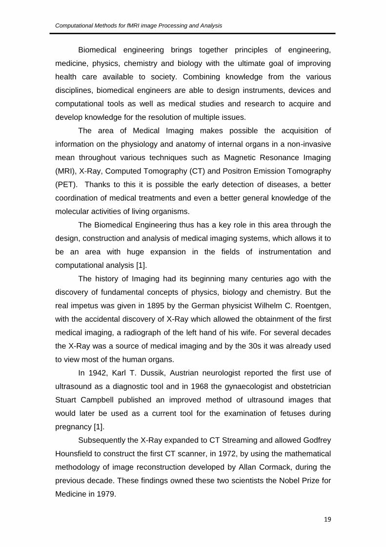
In the early 80's MRI was considered as a new way to take pictures
inside the human body and this spurred researchers to turn this technology in a
sophisticated and robust method of obtaining these images through the use of
scanners as the one in Figure 1.1.
Figure 1.1 – Siemens MAGNETOM Symphony 1.5T MRI System Scanner, USA. [1]
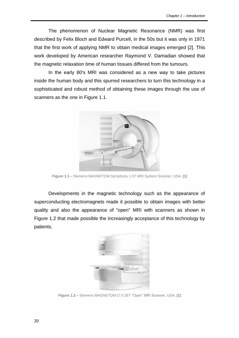
Developments in the magnetic technology such as the appearance of
superconducting electromagnets made it possible to obtain images with better
quality and also the appearance of "open" MRI with scanners as shown in
Figure 1.2 that made possible the increasingly acceptance of this technology by
patients.
Figure 1.2 – Siemens MAGNETOM C! 0.35T ”Open” MRI Scanner, USA. [1]

Computational Methods for fMRI image Processing and Analysis
21
In 1990, Seiji Ogawa, Japanese biophysical, discovered in works with the
partnership of AT & T's Bell Laboratories, that deoxyhemoglobin (dHb) when
under the influence of a magnetic field, increased the strength of the field in its
vicinity while the oxyhemoglobin (HbO2) did not. It was the discovery of this
phenomenon that led to the development of Functional Magnetic Resonance
Imaging (fMRI), which allowed the acquisition of images of functioning and the
study of their various functions.
The improvement of these technologies has also been possible with the
development of computational analysis area, by creating increasingly
sophisticated algorithms that enable the extraction of structural and functional
information for volumetric measurement, processing, display and analysis of
images [1].
1.1. Motivations and Goals
The Medical Imagiology field has, along the years, been gaining a big
relevance. Its development has evolved at such fast pace that the knowledge in
the anatomy and physiology of the human body became increasingly fast,
detailed and less expensive. Alongside this development, the technological
developments, mainly the computational ones, allowed the evolution of tools
and algorithms increasingly faster and more objective.
The fMRI studies and developments allowed the acquisition of
knowledge inherent to the technic and also to the image processing tools
needed during the development of this thesis.
Considering these aspects the goals of this thesis were:
Learning how to acquire functional MRI scans;
Learn to analyse the functional MRI images of the brain;
Acknowledge the theory of image processing (correction of motion,
co-registration, segmentation, etc.);
Knowing how to work with FMRIB Software Library (created by de
Analysis Group, FMRIB, Oxford, UK) (FSL), and the Statistical
Parametric Mapping (SPM) tool of MATLAB (created by members
and collaborators of the Wellcome Trust Centre of Neuroimaging);

Chapter 1 – Introduction
22
Calculate the centre of mass of the activating zone - Varying the
threshold values and measure the centre of mass for each case,
reaching an average value for the activation;
Study the automatic segmentation of the target lesion and study the
possibility of having to make a manual segmentation in some cases;
Determine in a three-dimensional volume the shortest distance
between the mass centre of the activation zone and the edge of the
lesion;
1.2. Dissertation overview
The following chapters present the theoretical and practical research
done during the development of this thesis. It is structured in six more chapters
that are briefly explained here:
Chapter 2 – The Brain: in this chapter a description of the brain is
provided. Hence, the chapter starts with the explanation of the brain
anatomy, followed by the physiologic events that happen in this
organ. Then, the chapter presents a description of the brain
activation areas and their functions and subsequently the cancer
pathologies more frequent in this organ and the diagnose criteria
chosen by doctors.
Chapter 3 – Magnetic Resonance Imaging: this chapter is a
presentation of the MRI technique explaining the physical principles
and instrumentation required for its use. Thereafter is explained the
process of mapping the MRI signal as well as the formation,
production methods and properties of the images from this
technique, and finally its main purpose applications.
Chapter 4 – Functional MRI: this chapter aims to explain the
technique of functional magnetic resonance imaging and its
principles, scanning methodologies, explain how to process an
experimental study of fMRI and how this technique is used for the
study of brain tumours.

Computational Methods for fMRI image Processing and Analysis
23
Chapter 5 – Image Processing and Analysis: here is explained the
complete procedure of analysis and processing of images used in
this work. It was intended to clarify the methods of pre-processing,
enhancement, segmentation and feature extraction to be used and
their subsequent application to fMR images.
Chapter 6 – Implementation, results and discussion: at this stage
is presented the software’s used throughout this thesis, their
operating mode, the more practical aspects of their implementation
and the data base of images used, and is explained all the
implementation of the practical part of the thesis, as well as their
results and their consequent discussion.
Chapter 7 – Conclusions and future perspectives: finally we
present the final conclusions, as well as the possible future prospects
of implementing an automatic method for the analysis and
measurement of brain tumours and their distance to the areas of
brain activation.
1.3. Major contributions
The major contribution of this thesis was to develop a method, using two
different software’s, for measuring the distance between the centres of mass of
brain activation areas and of the nearest edge of a brain tumour, and
comparison of both approaches, diagnosed in fMRI clinical exams, in order to
obtain a quantitative value to provide to the surgeon for surgical planning.

24
2. The Brain
2.1. Introduction
2.2. Anatomy and Physiology of the brain
2.3. Brain Activation Areas
2.4. Brain Tumours
2.5. Treatment Options
2.6. Summary

Computational Methods for fMRI image Processing and Analysis
25
2.1. Introduction
This chapter aims to give a brief explanation of the anatomy and
physiology of the brain, the most complex and vital organ, centre of the human
central nervous system, as well as their areas of activation and functions. Some
fundamental knowledge about brain tumours will also be presented, necessary
for the study in question.
2.2. Anatomy and Physiology of the brain
The human brain, shown in Figure 2.1, is the principal organ of the
central nervous system and the control centre of many voluntary and
involuntary activities of the body and as such is responsible for actions as
complex as thinking, memory, emotion and language. In the adult this organ
may have about 12 billion neurons (nerve cells).
Figure 2.1 – Medial aspect of the brain and brainstem [3]
It is divided into two hemispheres, left and right, where the functional
areas are differentiated, however there is no general agreement on the
definition and marking of the boundaries between each of these areas and the
absence of these anatomical definitions leads to the existence of several
subdivisions of the cerebral cortex. The left hemisphere is responsible for
logical thinking and communicative competences, with highly specialized areas

Chapter 2 – The Brain
26
such as Broca's area (B), responsible for motor speech, and Wernicke's area
(W) responsible for verbal comprehension, while the right hemisphere is
responsible for symbolic thought and creativity. The corpus callosum, located
deep in the sagittal fissure, is the structure that connects the two cerebral
hemispheres and is responsible for the exchange of information between
different areas of the cerebral cortex. The motor cortex is responsible for the
control and coordination of voluntary movements. The motor cortex of the left
hemisphere controls the right side of the body and the motor cortex of the right
hemisphere controls the left side of the body. The premotor cortex, responsible
for the motor learning and the precision movements, is located in front of the
area of the motor cortex. The cerebellum is primarily responsible for the overall
coordination of motor skills and balance. The axis formed by the adeno-
hypophysis and hypothalamus, is responsible for the homeostatic functions of
the organism (cardio-respiratory, circulatory, etc.).
The cerebral cortex is divided into four areas called cerebral lobes, with
differentiated and specialized functions:
The frontal lobe, located in the forehead, includes the motor cortex, the
premotor and the prefrontal cortex and is responsible for planning actions
and movements as well as functions that may include abstract and
creative thinking, fluency of thought and language, emotional and
affective responses, will and selective attention;
The occipital lobe, in the neck region, is covered by the cerebral cortex,
also referred to as the visual cortex, and consists of several sub-areas
specialized on processing the colour vision, movement, depth and
distance;
The parietal lobe, at the top centre of the head comprises two
subdivisions - the anterior designated by somatosensory cortex, with the
sensations related functions (touch, pain, temperature, etc.). And
posterior which is a secondary area which analyses, interprets and
integrates the information received by the previous area;
And temporal lobes, in the lateral regions of the head above the ears,
that have as main function the processing of auditory stimuli.

Computational Methods for fMRI image Processing and Analysis
27
There is another map also widely used, based on the subdivision of the
cerebral hemispheres in about 50 cytoarchitectonic areas (Figure 2.2), by
Korbinian Brodmann's, which are divided into five major functional areas [4]:
Limbic;
Paralimbic;
Heteromodal association;
Unimodal association;
Primary sensory-motor.
Figure 2.2 – Lateral (on top) and medial (on bottom) views of the cerebral hemispheres [4]

Chapter 2 – The Brain
28
2.3. Brain Activation Areas
As it is known the cerebral cortex, with 2-4 mm of thickness, composed
by an enormous number of neurons and their interconnections, is organized into
lobes and is the main responsible for higher and complex functions such as
sensory perception, memory, consciousness, attention, thinking, language,
movement and also emotions.
For a better understanding, the cerebral cortex is classified by function
into two different areas:
The motor control areas – located in both hemispheres of the cortex they
are responsible for the generation of movement. These areas are the
primary motor cortex, which is located in the pre-central gyrus, and the
premotor and motor areas (responsible for the staging of motor
functions). Figure 2.3 shows the topographic organization of the motor
cortex (the right half of the motor area controls the left side of the body,
and vice versa). There is also the Broca area or the speech motor area
(which communicates with the premotor and motor areas to determine
the speech muscular movements).
Figure 2.3 – Topographic organization of the primary motor cortex [5]

Computational Methods for fMRI image Processing and Analysis
29
The sensorial control areas – where the impulses responsible for senses
are received and interpreted. The senses that are detected are
responsible for smell, taste, hearing, vision and balance and somatic as
touch, temperature, pressure, pain and proprioception. The areas
responsible for this are the primary somatosensory cortex
(topographically organized in Figure 2.4), the areas of taste, the olfactory
cortex, primary auditory cortex, the primary visual cortex and association
areas or secondary (somatosensory, auditory and visual). And there is
also the Wernicke's sensory speech area (responsible for understanding
and formulating speech) [4].
Figure 2.4 – Topographic organization of the primary somatosensory cortex [5]
Figure 2.5 shows a representation of these anatomical areas in the left cortex.
Figure 2.5 – Functional regions representation of the left side of the cerebral córtex [6]

Chapter 2 – The Brain
30
Other important functions, but whose areas are not as well defined, are
the ones responsible for memory (temporal lobe) and for intelligence,
judgment and behaviour (frontal lobe) as shown in Figure 8 [7].
Figure 2.6 – Important functional areas of the brain [8].
2.4. Brain Tumours
By definition, a brain tumour is an abnormal growth of cells in the brain
tissues, inside the cranium, and according to Cancer Research UK, it is
estimated that every year there are almost 445000 news cases of brain tumours
worldwide [9].
These tumours are classified according to their origin. They are termed
primary, if they begin to grow directly in the brain; otherwise they are secondary,
if they spread to the brain from somewhere else in the body.
Primary brain tumours can be classified according to the type of tissue
that origins it, they do not spread to other body sites, and can be malignant or
benign. The most common ones are gliomas, which begin in the glial tissue and
according to some histology statistics there are:
Glioma 50,3%;
Glioblastoma 52%;
Astrocytoma 26%;
Oligodendroglioma, Ependymoma, etc 22%;
Meningioma 20,9%;

Computational Methods for fMRI image Processing and Analysis
31
Pituitary 15%;
Acoustic Neuroma, Nerve Sheath Tumors and Others 8% [9].
Secondary brain tumours, that are always malignant, are also known as
metastatic cancer as they are the result of the spreading of other cancers that
are growing somewhere else in the body and they are given the name of the
origin cancer and these are the most common types of brain tumours (10 to
15% of cancer patients develop metastatic cancer to the brain). The derivations
of these metastatic cancers percentage wise are:
Lung 35%;
Breast 20%;
Melanoma 10%;
Renal Cell 10%;
Colon 5% [9].
These two types of tumours are potentially disabling and life threatening
duo to the limited space inside the skull. Their growth increases intracranial
pressure, and may cause edema, reduced blood flow, and displacement, with
consequent degeneration, of healthy tissue that controls vital functions [10].
2.5. Treatment Options
Normally there is not one single procedure, it depends on the type, size
and location of tumour, but for a good treatment plan there are some standard
options like:
Surgery;
Radiation;
Radiosurgery;
Chemotherapy;
Other option (ex: clinical trials).
When possible, the most recommended approach is the surgical
removal, always maintaining the constraints of preservation of neurologic

Chapter 2 – The Brain
32
functions and considering a previous evaluation of the patients health and
surgical risks.
For high-grade gliomas the most common approach is radiation therapy.
Chemotherapy is a treatment option that is normally an addition to other
treatments like surgery and radiation, especially for malignant gliomas.
For metastatic brain tumours there is a management approach that
involves a combination of multiple treatments such as: corticosteroids,
anticonvulsants, radiation therapy, radiosurgery and surgical resection [11].
2.6. Summary
The brain, as fundamental to human functioning organ is of extreme
importance and the control centre of the human body, responsible for the
control of the voluntary and involuntary activities that it preforms. It is divided in
two hemispheres, each responsible for different functions. The more complex
functions are controlled by the cerebral cortex, where the motor control and the
sensorial control areas are located.
So in order to prevent damage to this organ and its functions, when
lesions occur, such as tumours, that could influence its performance, the
diagnosis and treatment is fundamental and indispensable.

33
3. Magnetic Resonance Imaging
3.1. Introduction
3.2. Technical principles
3.2.1. Instrumentation
3.2.2. Physics
3.2.3. MR signal
3.3. MR images
3.4. Other techniques and applications
3.5. Summary

Chapter 3 – Magnetic Resonance Imaging
34
3.1. Introduction
Magnetic Resonance Imaging (MRI) is an imaging technique capable of
producing tomographic images of internal physical and chemical characteristics
of a given body by external measurement of magnetic resonance signals.
Tomography is a very important area of imaging, the Greek word tomos
meaning "cut" but this enables obtaining images from inside the body without
actually cutting it. Thus with the use of an MRI scanner is possible to obtain
images and data sets representative of the multidimensional spatial distribution
of a given physical quantity measure [12].
3.2. Technical principles
With the use of Magnetic Resonance Imaging technics it is possible to
generate sectional 2-dimensional (2D) images with any orientation, volumetric
3D images and even 4D images of the spatio-spectral or spatio-temporal
distributions. Another special feature of this technology is the nature of the
signals used to form images since, unlike other technologies, it does not rely on
particles with radiation to generate the signals received [12].
3.2.1. Instrumentation
The basic components of an MRI scanner are shown schematically in
Figure 3.1:
Figure 3.1 – Typical MRI system organization [13]

Computational Methods for fMRI image Processing and Analysis
35
These instruments have static magnetic fields, uniform and strong (the
strength can vary between 0.2T and 3T in clinical use) with three sets of coils,
which have amplifiers and devices associated for correcting the current,
necessary for spatial coding of the examining patient for producing a time
varying magnetic gradient. The Radiofrequency (RF) transmitter transmits and
receives the coils and amplifiers and the RF receivers are used for excitation of
the nuclei and to receive the signals. The computer is used to control the
scanner and to process and present the results (images, spectra, etc.). They
also contain other devices and equipment for patient and safety systems
monitoring [14].
The magnet provides a stable and uniform magnetic field (B0) (Figure
3.2);
The field B0 of these scanners can be generated by resistive
electromagnets, permanent magnets or superconducting magnets, being theses
the most common and which due to the superconducting technology requires
an own cooling system with liquid helium.
Figure 3.2 – Formation of a superconducting magnet scheme [2]
The RF transmitter sends pulses of RF to the sample;
For the activation of nuclei this system that emits the signals consists of
the RF transmitter itself, in a power amplifier and RF coils of transmission. A
crystal that oscillates at a frequency of precession constitutes the transmitter
itself.
The gradient system generates time-varying magnetic fields;

Chapter 3 – Magnetic Resonance Imaging
36
It is this gradient system that is responsible for the ability of spatial
coding the detected signals for the formation of images. This is due to the ability
to locally control the magnetic field and to the use of three coils, which imposes
linear variations in the magnetic field in any of the Cartesian directions.
The detection system produces the output signal;
Its main function is to detect and generate the output signal to be
processed by the computer and its structure is presented in accordance with the
block diagram of Figure 3.3.
Figure 3.3 – Block diagram of detection system [13]
Here the receiving coil will act as an antenna to the floating nuclear
magnetization of the sample and converts it into floating output voltage V(t). The
coil is connected to a matching network that establishes the connection to the
preamp to maximize the energy transferred to the amplifier and introduces a
phase alternator for the signal. The preamp is a low noise amplifier that
amplifies the signal and transfers it to a quadrature phase detector. This
detection circuit receives the MR V(t) signal and the reference signal and
multiplies it to obtain just an output. It also has a low pass filter for the removal
of all components except the ones centred at zero. Lastly the signal is
processed by an Analog-Digital (A-D) converter that transforms it in a series of
data to be analysed in the computer.
The imager system includes the computer for reconstruction and display
of images (Figure 3.4) [13];

Computational Methods for fMRI image Processing and Analysis
37
Figure 3.4 – Siemens Operation console of the MRI scanner [2]
In Figure 3.5 one can see how all these components are organized within
an MRI scanner.
Figure 3.5 – Scheme of construction of an MRI scanner [15]
3.2.2. Physics
The protons and neutrons constituents of atomic nuclei possess a
property called spin angular momentum (Φ) with magnitude and direction and
which underlies the phenomenon of Nuclear Magnetic Resonance (NMR). This
angular momentum or spin core may be considered as a result of rotational
movement of the nucleus around its own axis which is illustrated in Figure 3.6.
Hydrogen (1H) is the most abundant element in the body and hence the
element of greatest interest for obtaining anatomical MR images enabling a
stronger MRI signal.

Chapter 3 – Magnetic Resonance Imaging
38
Figure 3.6 – Representation of the angular momentum of the nucleus [2]
Being the nucleus a charged particle, the spin is accompanied by a
magnetic moment vector (μ) whose magnetization field representation is in
Figure 3.7, and whose relationship with the spin angular momentum is given by
the expression:
(3.1)
where γ is the gyromagnetic ratio which is a particular characteristic of
the nuclei.
Figure 3.7 – Microscopic representation of the magnetization of a nucleus [2]
Table 1 shows the values of the gyromagnetic ratio of some common
elements [2].
Table 3.1 – Values for the Gyromagnetic Ratio
Gyromagnetic Ratio (MHz/T)
1H 42.58
13C 10.71
19F 40.05
31P 11.26
In the MRI the signal obtained is produced by the magnetic field of 1H,
being this a signal too small to induce a current which can be detected by a coil.
Computational Methods for fMRI image Processing and Analysis
39
Thus it becomes necessary the alignment of the protons so that it is possible to
produce a magnetic moment large enough to be detected.
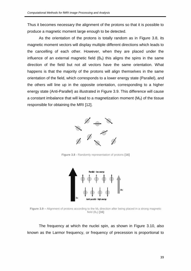
As the orientation of the protons is totally random as in Figure 3.8, its
magnetic moment vectors will display multiple different directions which leads to
the cancelling of each other. However, when they are placed under the
influence of an external magnetic field (B0) this aligns the spins in the same
direction of the field but not all vectors have the same orientation. What
happens is that the majority of the protons will align themselves in the same
orientation of the field, which corresponds to a lower energy state (Parallel), and
the others will line up in the opposite orientation, corresponding to a higher
energy state (Anti-Parallel) as illustrated in Figure 3.9. This difference will cause
a constant imbalance that will lead to a magnetization moment (M0) of the tissue
responsible for obtaining the MRI [12].
Figure 3.8 - Randomly representation of protons [16]
Figure 3.9 – Alignment of protons according to the M0 direction after being placed in a strong magnetic field (B0) [16]
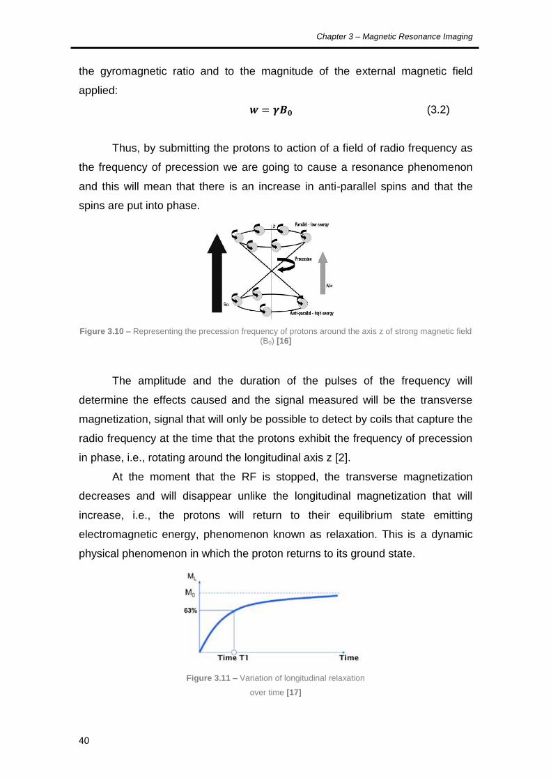
The frequency at which the nuclei spin, as shown in Figure 3.10, also
known as the Larmor frequency, or frequency of precession is proportional to
Chapter 3 – Magnetic Resonance Imaging
40
the gyromagnetic ratio and to the magnitude of the external magnetic field
applied:
(3.2)
Thus, by submitting the protons to action of a field of radio frequency as
the frequency of precession we are going to cause a resonance phenomenon
and this will mean that there is an increase in anti-parallel spins and that the
spins are put into phase.
Figure 3.10 – Representing the precession frequency of protons around the axis z of strong magnetic field (B0) [16]
The amplitude and the duration of the pulses of the frequency will
determine the effects caused and the signal measured will be the transverse
magnetization, signal that will only be possible to detect by coils that capture the
radio frequency at the time that the protons exhibit the frequency of precession
in phase, i.e., rotating around the longitudinal axis z [2].
At the moment that the RF is stopped, the transverse magnetization
decreases and will disappear unlike the longitudinal magnetization that will
increase, i.e., the protons will return to their equilibrium state emitting
electromagnetic energy, phenomenon known as relaxation. This is a dynamic
physical phenomenon in which the proton returns to its ground state.
Figure 3.11 – Variation of longitudinal relaxation
over time [17]

Computational Methods for fMRI image Processing and Analysis
41
There are two types of relaxation, the longitudinal relaxation described by
an exponential curve characterized by the time constant T1, during which
protons are again aligned with the magnetic field. The curve illustrated in Figure
3.11 represents the variation of longitudinal relaxation over time, where one can
see that T1 represents the time required for the longitudinal magnetization (ML)
to recover 63% of its initial value (M0). The transverse relaxation is described by
an exponential curve characterized by the time constant T2, which comes down
to the exit of the protons of its phase state and the curve represented in Figure
3.12 shows the variation of magnetization in the transverse plane over time,
where T2 represents the time required for the transverse magnetization (MXY) to
reach 32% of its initial value [17]. The transverse relaxation is more rapid than
the longitudinal relaxation and these values are not related to magnetic field
strength.
Table 2 shows some values of relaxation times, at the precession
frequency of 20 MHz:
Table 3.2 – Approximate values of T1 and T2 for different tissues [18]
T1 (ms) T2 (ms)
Blood 1200 200
Muscle 500 35
Fat tissue 200 60
Water 3000 3000
White matter 790 90
Gray matter 920 100
Cerebrospinal liquid 4000 2000
Figure 3.12 – Variation of magnetization in the transverse plane over time [17]
Chapter 3 – Magnetic Resonance Imaging
42
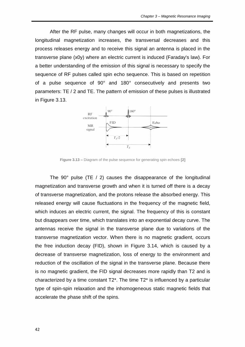
After the RF pulse, many changes will occur in both magnetizations, the
longitudinal magnetization increases, the transversal decreases and this
process releases energy and to receive this signal an antenna is placed in the
transverse plane (x0y) where an electric current is induced (Faraday's law). For
a better understanding of the emission of this signal is necessary to specify the
sequence of RF pulses called spin echo sequence. This is based on repetition
of a pulse sequence of 90° and 180° consecutively and presents two
parameters: TE / 2 and TE. The pattern of emission of these pulses is illustrated
in Figure 3.13.
Figure 3.13 – Diagram of the pulse sequence for generating spin echoes [2]
The 90° pulse (TE / 2) causes the disappearance of the longitudinal
magnetization and transverse growth and when it is turned off there is a decay
of transverse magnetization, and the protons release the absorbed energy. This
released energy will cause fluctuations in the frequency of the magnetic field,
which induces an electric current, the signal. The frequency of this is constant
but disappears over time, which translates into an exponential decay curve. The
antennas receive the signal in the transverse plane due to variations of the
transverse magnetization vector. When there is no magnetic gradient, occurs
the free induction decay (FID), shown in Figure 3.14, which is caused by a
decrease of transverse magnetization, loss of energy to the environment and
reduction of the oscillation of the signal in the transverse plane. Because there
is no magnetic gradient, the FID signal decreases more rapidly than T2 and is
characterized by a time constant T2*. The time T2* is influenced by a particular
type of spin-spin relaxation and the inhomogeneous static magnetic fields that
accelerate the phase shift of the spins.

Computational Methods for fMRI image Processing and Analysis
43
Figure 3.14 – Free induction decay caused by the transverse relaxation [2]
The impulse of 180º (TE) puts the spins in phase and inverts the
inhomogeneous magnetic field and once applied with an RF with this pulse the
spins go into phase and the transverse magnetization reappears and increases.
After that, the spins move into a state of imbalance and the transverse
magnetization decreases. When this state is fully achieved, the 180º pulse is
sent and protons come back in phase. When switching off, the pulse of the 180º
signal is emitted in the form of echoes. The difference in signal intensity
depends on two factors, the Repetition Time (TR - which is the difference
between the signal intensity between T1 tissues using two consecutive pulses,
i.e. the difference between the longitudinal magnetization of different tissues)
and the Echo Time (TE - which is the time between the 90º pulse and the echo).
It could be chosen by the operator that indicates the type of the image (T1-
weighted image, proton density and T2-weighted image – Figure 3.15) [18].
Figure 3.15 – MR images of sagittal brain cross section (T2W – T2 weighted, T1W – T1 weighted, PD – proton density) [19]
But there are other important factors that are needed to form an image.
For an object slice:

Chapter 3 – Magnetic Resonance Imaging
44
The area that is acquired is the “field of view” – FOV, that is normally
considered to be squared;
The position is described by two-dimensions, the read-out (x) and the
perpendicular phase-encode (y) direction.
Considering an object with a certain thickness (d), this is divided into
volume elements (voxels) as shown in the Figure 3.16.
in which the transverse directions is FOV/N and d in the longitudinal
direction. The volume for each voxel is then given by:
⁄ (3.3)
The total magnetization vector of the voxel corresponds to the sum of all
magnetizations inside a voxel and the length of this vector for each voxel is the
brightness of a point in the image that is named pixel. The image is than
obtained by gathering all the pixels together [20]. For a 3D image, the volume
for each voxel is given by:
(3.4)
Considering the patient as in the position showed in Figure 3.17, the
magnetic field gradient will now be described along the z axis with:
(3.5)
The amplitude of the MR signal is proportional to the number of spins in
a plane perpendicular to the gradient and this is called frequency encoding. This
Figure 3.16 – Object slice divided into voxels [20]

Computational Methods for fMRI image Processing and Analysis
45
causes the resonance frequency to be proportional to the position of the spin
and with association to the correspondent spatial location z, becoming:
(3.6)
where B0 is the magnetic field and Gz is the magnetic field gradient along
the plane z.
Figure 3.17 – side view of selected of axial image plane locations [19]
The one-dimensional magnetic field gradient along the z axis in B0
indicates that the magnetic field is increasing in the z direction. Here the lengths
of the vectors represent the magnitude of the magnetic field. The symbols for a
magnetic field gradient in the x, y, and z directions are Gx, Gy, and Gz [19].
The large variety of available pulse sequences for imaging also reflects
the variety of goals of imaging in different applications, such as the identification
of pathological anatomy, and this requires a combination of sufficient spatial
resolution to resolve small structures and sufficient signal contrast between
pathological and healthy tissue to make the identification.
To obtain an image with many pulse sequences, the MR signal is
operated by manipulation of both the RF and the gradient pulses in many ways.
The RF pulses can be used as excitation pulses, to turn the magnetization from
the longitudinal axis to the transverse plane, generating a detectable signal and
as a refocusing pulse, to generate echoes of previous signals. The gradient
pulses are used to eliminate unwanted signal and to encode information about
the signals spatial distribution. Figure 3.18 shows a diagram with the pulse
sequences in an acquisition event.

Chapter 3 – Magnetic Resonance Imaging
46
Figure 3.18 – Pulse sequence diagram [21]
Another of the main concepts behind this phenomenon is the spatial
Fourier transform of the image, the k-space, which can be measured directly in
the MR image. This concept allows the determination of parameters and
features like the field of view (FOV), the spatial resolution and the speed of
acquisition.
The k-space selection determines the basic parameters of the image,
such as the FOV, spatial resolution, and speed of acquisition and the magnitude
of the local MR signal, determines whether an image will show useful contrast
between one tissue and another.
The Fourier transform theorem states that any function of position x, such
as a profile through an image I(x), can also be expressed as a function of
spatial frequencies S(k), that is a sum of sine and cosine waves of different
wavelengths and amplitudes that spread across all of x, where k is the inverse
of the wavelength and so small k-values correspond to low spatial frequencies
and long wavelengths. These two functions are related so that given one
representation; the other can be obtained by calculation of the Fourier
transform. Their mathematical relation can be seen in: [22].
∫
∫
(3.7)
Computational Methods for fMRI image Processing and Analysis
47
This k-space representation is given such an importance because indeed
is the S(k) that is actually measured and the I(x) is than reconstructed.
Now the image can be calculated by applying a 2D Fourier transform to
the data acquires, by having the distribution in space being represented in
terms of amplitudes of different spatial frequencies (k). So the MR image
directly maps the k-space because the 2D Fourier transform will relate the
image to the k-space representation.
In conclusion, the signals described above must be Fourier transformed
to obtain the image representative of the location of spins. So during the MRI
signal acquisition the phase and frequency encodings will vary and the
correspondent signal will be recorded and used to fill the k-space. The phase
encoding gradient will position the spin system at a specific line in the k-space
array and the frequency encoding gradient will allow the movement of the spin
system across that k-space line as function of the time.
Once the k-space is filled, the Fourier transformed data will be displayed
as an image by conversion of the peaks to intensities of pixels representing the
tomographic image.
3.3. MR images
MR images, after acquired, are usually stored and manipulated as a grid
or matrix of points representing a slice, 2D image. These are matrices of pixels
with M rows and N columns, where every pixel corresponds to a voxel and their
information is normally codified in a digital image format.
The most typical format used for this is the Digital Imaging and
Communications in Medicine, also known as DICOM-files. This is a very useful
format because in addition to the MR image itself, it stores also information
about the position and the orientation of the image regarding the MR scan and
the patient.

Chapter 3 – Magnetic Resonance Imaging
48
For a 3D volume image, the scan acquires several slices, as shown in
Figure 3.19, creating a 3D matrix with size M x N x K, where K represents the
number of slices [12].
Figure 3.19 – MR image sequence with 5.5 mm spacing between slice [12]
But in real clinical practice, making images is an automatic process, with
all gradients and timings pre-programmed in the MRI software. So this should
create an ideal imaging technique with a rapid acquisition of data to provide
good temporal resolution, high spatial resolution to resolve fine details of
anatomy, and a high signal to noise ratio (SNR) to distinguish the tissues of
interest by differences in the MR signal they generate.
Yet this does not happen. As spatial resolution is improved, the smaller
image voxel generates a weaker signal relative to the noise. So high resolution
images, with voxel volumes much less than 1 mm3, could be acquired with
standard equipment, what would lead to a Signal-to-Noise Ratio (SNR) so
degraded that some anatomical information would be lost and as the voxel size
decreases, the total number of voxels in the image increases, requiring a longer
imaging time to collect the necessary information [22].

Computational Methods for fMRI image Processing and Analysis
49
Artefacts
Since it is almost impossible to ascertain the optimal conditions seen
above, the images suffer some distortion, which are due to artefacts. Table 3
shows a list of some of these artefacts and these will be described next.
Table 3.3 – List of some artefacts that influence MRI [23] [22] [12]
Type Artefact Cause
Patient
related Motion
Voluntary or involuntary movements of
the patient during the acquisition
Signal
processing
related
Chemical Shift
Mis-registration between the relative
positions of two tissues with different
resonance frequencies under an external
magnetic field
Partial Volume Large voxel size
Gibbs Phenomenon
Images with bright or dark lines adjacent
to sharp boundaries duo to high spatial
frequencies
Hardware
related
Signal Noise Bad RF shielding and operation of the RF
coil and presence of metal in the patient
B0 Inhomogeneity B0 field distortion normally duo to metal
objects in the patient
Motion
During image acquisition, any movement performed by the patient, from
the smallest movements of the head to the pulsing of blood vessels, will
generate motion artefacts. These are responsible for a distorted analysis of the
data series and not always their correction is possible through post-processing
techniques. So, the application of realignment algorithms to the captured
images to allow the obtainment of the geometric transformation function that is
best suited to minimize differences between the images [22].
Chapter 3 – Magnetic Resonance Imaging
50
Chemical Shift
It occurs at fat/water interface because of the frequency difference
between the two components when under the influence of the external magnetic
field. The protons of the fat tissue resonate at a slightly lower frequency then
the water protons due to their different molecular structure.
The number of pixels affected by this artefact will depend of the
frequency difference in Hz between the 2 components, the total receiver
bandwidth and the number of readout data that cover the FOV. It can be
determined and minimized shifting the phase-encoding and frequency-encoding
gradients and examining the result or through the use of fat suppression
techniques [23].
Partial Volume
This artefact occurs when the size of the image voxel is larger than the
size of the tissue of interest to be imaged, manly when multiple tissue types are
comprised within a single voxel. That is, if a small structure is entirely contained
within the slice thickness along with other tissue that has a different frequency,
the resultant image will then have a signal correspondent to an average signal
of the frequencies of both structures and this will cause a reduction of the
contrast and loss of spatial resolution. So a solution for this problem could be a
usage of a smaller pixel size or of a smaller slice thickness [23].
Gibbs Phenomenon
This artefact is represented by the appearance of a series of lines
parallel to a sharp intensity edge present in the image, normally borders of an
abrupt intensity change which is caused by an incomplete digitization of the
echo; in other words, where the signal has not decayed to zero by the of the
acquisition window.
The Gibbs artefact can also be known as the truncation artefact because
it results from the truncation of sampling in k-space, meaning an under-
sampling of high spatial frequencies.
The methods used to solve this can be using a larger image matrix or
filtering the k-space data prior to the Fourier transform [22].

Computational Methods for fMRI image Processing and Analysis
51
Signal Noise
This is referred to artefacts generated from unwanted signals resulting
from multiple sources, normally from nearby electronic equipment that emit RF
radiation that is captured by the head coil, causing significant noise in the
acquired image [24].
B0 Inhomogeneity
This type of interference leads to errors in the mapping of the tissue
because it can cause spatial and intensity distortions. The spatial distortion
results from a long-range field gradient in B0 that causes the spins to resonate
at Larmor frequency different from the required. The intensity distortion is
caused due to greater or smaller field homogeneity in a certain region than the
imaged object [12].
3.4. Other techniques and applications
Some of the existing applications of this technology are:
Standard MRI;
Echo-planar imaging;
Fast Imaging with Steady-state Precession (FISP);
Half Fourier Acquisition Single-shot Turbo spin Echo (HASTE);
Magnetic Resonance Angiography;
Magnetic Resonance Spectroscopy;
Functional MRI.
3.5. Summary
Magnetic Resonance Imaging produces tomographic images of internal
physical and chemical characteristics of a given body by obtaining images and
data sets representative of the multidimensional spatial distribution of a given
physical quantity measure and these can be 2-dimensional (2D) sectional
Chapter 3 – Magnetic Resonance Imaging
52
images with any orientation, volumetric 3D images and even 4D images of the
spatio-spectral or spatio-temporal distributions. These are captured with a
scanner that has a static magnetic fields, uniform and strong and a computer
used to control it and to process and present the results. This scanner analysis
the Hydrogen composition of the body because it enables a stronger MRI
signal.
The signal also depends on the Repetition Time and the Echo Time
which can define the type of the image that is obtained and of a large variety of
pulse sequences depending on the goals of imaging for the different
applications, such as the identification of pathological body.
Another important concept that was acknowledged was the k-space
selection responsible for some basic parameters of the image, such as the
FOV, spatial resolution, etc., and the artefacts that affect the images that can
cause some distortion.

53
4. Functional MRI
4.1. Introduction
4.2. Principles
4.3. Guidelines for fMRI experimental studies
4.4. Scanning methodologies
4.5. Analysis of fMRI studies
4.6. Limitations
4.7. Summary

Chapter 4 – Functional MRI
54
4.1. Introduction
The brain, like any other organ in the body requires a steady supply of
oxygen in order to metabolise glucose to provide energy. This oxygen is
supplied by the component of blood called haemoglobin that has magnetic
properties which can be measured in a certain volume of oxygen present in the
brain [17]. This volumetric dependency gave rise to a method for measuring the
brain activation using MRI, commonly known as Functional Magnetic
Resonance Imaging (fMRI) which will be approached in this next chapter.
4.2. Principles
The functional Magnetic Resonance Imaging is an application of the
Magnetic Resonance Imaging referred to the use of this technology to detect
localized changes in blood flow and blood oxygenation in the brain that occur in
response to neural activity.
The concept that the cerebral blood flow could reflect neuronal activity
began in 1890 with experiments carried out by Roy and Sherrington and this
became the basis of all brain imaging techniques based on hemodynamic. In
the last decades this technique has been greatly developed with the goal of
mapping the human brain and has been extensively used to investigate the
brain functions such as vision, language, motor and cognitive [22].
In 1990 Ogawa reported, based on their study in rat brains, that the
mapping of functional brain was possible due to the BOLD effect (Blood
Oxygenation Level Dependent) based on changes of deoxy-hemoglobin (dHb),
where this acts as an contrasting parametric agent and whose local
concentration changes in the brain leads to an increase in the intensity of the
MRI signal [25].
Although the mechanisms which connect neuronal activation and brain
physiology are still the subject of many studies, it is known that neuronal
activation leads to an increased consumption of ATP (adenosine triphosphate),
which implies an increase in oxygen demand and to fill this necessity an
increase in local blood flow occurs and these physiological changes are

Computational Methods for fMRI image Processing and Analysis
55
essential for fMRI. Thus, crossing the capillaries network, the oxy-hemoglobin
(HbO2) will release the oxygen it carries, becoming deoxy-hemoglobin (dHb),
whose paramagnetic properties act to locally intensify the effects of external
magnetic field. Therefore, to suppress this lack of O2, there is an increase of
local blood flow and volume, which leads to a further decrease in the
concentration of dHb compared to basal level, and these changes in
concentration of dHb act as contrast agent [24] [26].
Thus, according to Pauling & Coryell dHb is paramagnetic (attractive),
that is, magnetizes in the same direction of the magnetic field to which it is
exposed and HbO2 is diamagnetic (repulsive) and these magnetic properties
have a direct effect on the intensity of the detected signal in neural active
regions. It can be verified that an increase in concentration of HbO2 in blood
flow will cause an increase in intensity of the captured signal and an opposite
situation, namely in the presence of a higher concentration of dHb will lead to a
decrease in local intensity due to the realignment of T2 and T2*. This occurs
because the events that start with the increase of electrical activity and
modulates the neurovascular response alter the MRI signal in time and produce
the hemodynamic response function [27].
The fMRI techniques have evolved very rapidly over the past few years
along with the development of analytical methods that can detect changes in
neural activity. Therefore one of the main applications of fMRI is related to the
field of neuroscience to allow a better study of the brain mechanisms as
complex as perception, emotions, behaviour and pain, being of great interest to
achieve quantitatively descriptions of these functions as well as qualitatively.
The fMRI fits well with these objectives because it involves a set of
techniques that enables the exploration of the susceptibility of MRI signals to
the physiological processes associated with brain activity [22].
4.3. Guidelines for fMRI experimental studies
For the analysis of fMRI a number of techniques derived from methods of
processing and statistical analysis has been used. These can be classified as
derived hypothesis and based on models or as derived data and exploratory.

Chapter 4 – Functional MRI
56
The methods include model-based analysis of variance (ANOVA) and
correlational methods and methods derived from data include principal
component analysis (PCA) and Independent Components Analysis (ICA), all of
which methods have as common factor the ability to identify the more
meaningful areas of brain activation in a patient [28].
The fMRI studies are highly dependent on cerebral hemodynamic
changes and for the organization of these are necessary to take into account
the spatial and temporal characteristics of these hemodynamic effects. The
spatial characteristics resulting from cerebral vasculature and the temporal
characteristics relate to the inherent delay of signal changes in response to
neural activity and the hemodynamic changes resulting dispersion over time.
Based on the temporal characteristics of the hemodynamic phenomena
we can also classify the fMRI studies in [29]:
Delineation blocks, where the experience is performed in continuous
mode in blocks of time (typically lasting 20-60 sec) and whose purpose is
to create a "steady state" of neuronal and hemodynamic changes. This is
a good method for detecting small changes in brain activity. A schematic
representation can be seen in Figure 4.1;
Delineation related with events uses temporal response patterns and
the hemodynamic response characteristics associated with the linear
application of multiple stimuli. These last are applied individually and in
random order and measure the hemodynamic response to each of them.
This method may further divided into:
Design of spaced single study (with long intervals between stimuli
and are used in order to allow that in the end of each stimulus the
hemodynamic response returns to its resting state);
Design of fast single study (which takes advantage of the property
of linearity and superposition of the hemodynamic response).

Computational Methods for fMRI image Processing and Analysis
57
For these studies is also of extreme importance to know how to
recognize the key variables to consider such as spatial resolution, temporal
resolution, cerebral coverage and signal to noise ratio (SNR), so that they can
be conveniently manipulated to obtain the desired results. Thus, to obtain a very
high spatial resolution is necessary to reduce the temporal resolution, limit the
coverage and reduce cerebral SNR.
However we must also consider other important aspects associated with
these techniques, such as the extremely high financial costs and restrictions on
patient safety [30].
For the BOLD fMRI studies, the most efficient design is the block design.
According to Matthews and Jezzard “this design uses long alternating periods,
during each of which a discrete cognitive state is maintained”. There has to be
at least two different states alternating during the experiment in order to prevent
that patient related artefacts or scanner sensitivity influence different impacts on
the signal responses from both states [31].
4.4. Scanning methodologies
In an fMRI clinical study a large series of images is acquired while the
patient is asked to do some tasks that make the brain activity shift between two
or more well-defined states. The experimental procedure for the data acquisition
can be described in a few general steps:
the patient lies down, without moving, in a MRI scanner;
Figure 4.1 – Experimental designs for fMRI studies (A – block
design, B – event-related design [29]

Chapter 4 – Functional MRI
58
next is the acquisition of the anatomical/structural scans of the brain (for
about 6-15 minutes);
then is a series of tests to collect the functional data between 3 to 10
minutes each (in these tests the patient will perform a few tasks that were
pre-designed by the clinician. During the tests the scanner records the
BOLD signal throughout the brain every each seconds.
This whole exam can take approximately 60 to 90 minutes and during it,
several functional images are recorded each containing a large number of
voxels, which constitute the time series of BOLD signals.
After this acquisition process the images are analysed with the goal to
identify the brain areas that are significantly active during the experimental
conditions compared to control conditions. This is made by correlating the
signal time series in each voxel of a slice with the known time series of the test.
[29].
4.5. Analysis of fMRI studies
The main goal in analysing functional imaging experiments is to identify
the voxels that present signal changes that vary with the changing in brain
states of interest on the acquired images.
The first step of this procedure is the pre-processing of the data
consisting of:
movement correction and realignment of the image series;
spin history correction associated to head movements;
spatial and temporal filtering;
global intensity normalization;
re-sampling of the data;
re-ordering of the data [32].
Then, after the pre-processing step is complete comes the model fitting
procedure where each voxel will be analysed in order to find voxel with time
series correlated with the experimental conditions. The common process is to
use mathematical functions to represent the BOLD response and estimate the
data parameters [33].
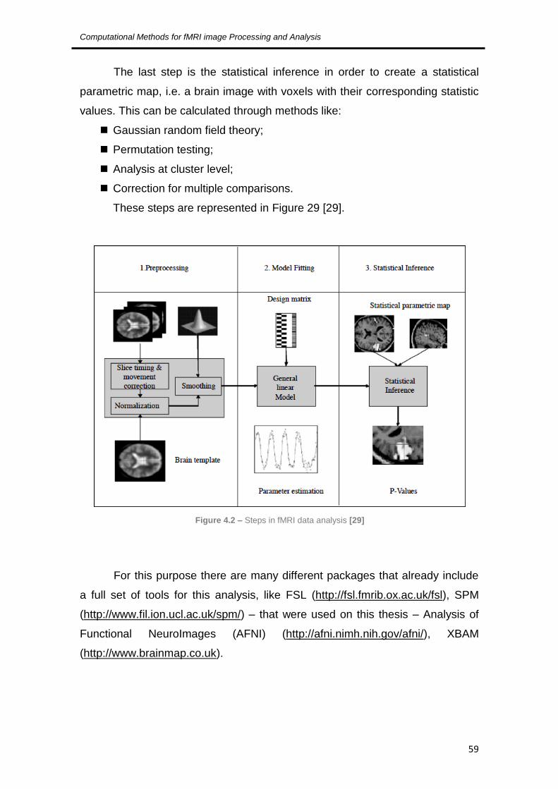
Computational Methods for fMRI image Processing and Analysis
59
The last step is the statistical inference in order to create a statistical
parametric map, i.e. a brain image with voxels with their corresponding statistic
values. This can be calculated through methods like:
Gaussian random field theory;
Permutation testing;
Analysis at cluster level;
Correction for multiple comparisons.
These steps are represented in Figure 29 [29].
For this purpose there are many different packages that already include
a full set of tools for this analysis, like FSL (http://fsl.fmrib.ox.ac.uk/fsl), SPM
(http://www.fil.ion.ucl.ac.uk/spm/) – that were used on this thesis – Analysis of
Functional NeuroImages (AFNI) (http://afni.nimh.nih.gov/afni/), XBAM
(http://www.brainmap.co.uk).
Figure 4.2 – Steps in fMRI data analysis [29]
Chapter 4 – Functional MRI
60
4.6. Limitations
Although fMRI is a very promising and useful technic it also presents a
few limitations that need to be considered, not taking into account the artefacts
referred in the previous chapter, inherent to this technic. These include:
Large amount of images to evaluate;
sensitivity to motion (patients head movements or brain microscopic
movements);
spatial and geometric uncertainty;
poor temporal resolution;
reduction of BOLD signal with proximity of brain lesions;
large amount
possible presence of false positives from the statistical analysis [34] [35].
4.7. Summary
The functional Magnetic Resonance Imaging is used to detect localized
changes in blood flow and blood oxygenation in the brain that occur in response
to neural activity and allows a better study of the brain mechanisms because it
involves a set of techniques that enables the exploration physiological
processes associated with brain activity. The studies developed to study this
phenomenon can be delineation blocks or delineation related with events that
take into account several key variables like spatial resolution, temporal
resolution, cerebral coverage and signal to noise ratio (SNR), so that they can
be conveniently manipulated to obtain the desired results. For a real fMRI
clinical study a large series of images is acquired while the patient is asked to
do some tasks that make the brain activity shift between two or more well-
defined states and in these the main goal is to identify the voxels that present
signal changes that vary with the changing in brain in order to obtain a statistical
inference to create a statistical parametric map of the activity correspondent to
the tasks preformed.

61
5. Image Processing and Analysis
5.1. Introduction
5.2. Image pre-processing – Artefacts removal
5.3. Image Enhancement
5.3.1. Spatial domain
5.3.2. Frequency domain
5.4. Image Segmentation and Feature Extraction
5.4.1. Edge-based segmentation
5.4.2. Thresholding
5.4.3. Region-based segmentation
5.5. Summary

Chapter 5 – Image Processing and Analysis
62
5.1. Introduction
For a fMRI study is necessary to acquire one or more series of functional
data (sequences of rapid MR), obtained during the performance of motor or
sensory stimuli or during the performance of paradigms, which are sets of
cognitive tasks, and acquisition of anatomical data (sequences of slow MR)
covering areas of interest which serve as reference for the structural
visualization of active functional areas. After this acquisition, the location and
characterization of brain regions activated by stimuli is made. This requires
several processing steps of the images since this process is subjected to the
influence of several types of artefacts that can adulterate the acquired images
[36].
According to Jenkinson & Smith [37] there is not only one protocol for the
analysis of images of fMRI; however there is a base sequence of steps for
processing images from fMRI:
1) Acquire and reconstruct the individual images;
2) Correct the time series phase for timing variations of the obtained
cuts;
3) Apply a motion correction to correct head movements;
4) Spatial smoothing of data to increase SNR;
5) Filter each voxel's time series to remove temporal variations and
high-frequency noise;
6) Perform the statistical analysis (through the generation of a
statistical parametric map - a SPM)
7) Thresholding of SPM to find the significant active regions.
5.2. Image pre-processing – Artefacts removal
The contrast due to the BOLD effect combined with fast acquisition
techniques, allows the visualization of certain brain processes. However, such
contrast changes are not directly visible, which implicates the use of
computational algorithms for the visualization of these same areas.
Computational Methods for fMRI image Processing and Analysis
63
Motion correction:
During image acquisition, any movement performed by the patient, from
the smallest movements of the head to the pulsing of blood vessels, will
generate motion artefacts. These are responsible for a distorted analysis of the
data series and not always their correction is possible through post-processing
techniques. So, the application of realignment algorithms to the captured
images to allow the obtainment of the geometric transformation function that is
best suited to minimize differences between the images [22].
One example of a possible approach is the use of Motion Correction
FMRIB’s Linear Image Registration Tool (MCFLIRT) algorithm used by the
software package FMRI Brain’s Software Library (FSL).
This algorithm is an image-similarity-based motion algorithm used on
fMR time-series images. It is based on optimization and registration techniques
from another fully automated tool for intra and inter-modal brain image
registration, the FLIRT (FMRIB’s Linear Image Registration Tool).
According to Jenkinson, M. et al, the algorithm, as in Figure 5.1, follows
the next steps:
1) loads the entire time-series;
2) sets the middle image (Vn) as the initial image;
3) 8-mm optimization by identity transformation between Vn and the
adjacent image (Vn+1);
4) search for the optimal transformation (T1) using the normalized
correlation cost function;
5) consider the previous result as the starting point and follow the
optimization for the next pair Vn, Vn+2;
6) 4-mm optimization between Vn and the results from the previous
optimization (as startup parameters);
7) 4-mm optimization with tighter tolerance between Vn and the results
from the previous optimization;
8) apply the transformation parameters to uncorrected images.

Chapter 5 – Image Processing and Analysis
64
Temporal correction
The obtainment of temporal data series is performed by the acquisition of
a cut at each time, which implies that different parts of the brain are not
analysed simultaneously and that the data cannot be considered as an instant
sample. Thus, for correcting this offset the data are adjusted through a
displacement range of each temporal series of voxel's which can be done by
applying an 1-D interpolation in the time domain or by applying a Fourier
transform [36].
Spatial smoothing
This step has as main goal the application of smoothing filters to reduce
the distorting effects possibly caused by the instrumentation or even the
physiological activity of the brain that can lead to the presence of noise. Thus
for this purpose one resorts normally to low-pass filters, such as the 3D
Gaussian filter, whose effects can be observed in Figure 5.2, to make a spatial
smoothing of the temporal series of the fMRI data [36].
Figure 5.1 – Representation of the previous algorithm process [37]

Computational Methods for fMRI image Processing and Analysis
65
Figure 5.2 – Applying a 3D smoothing Gaussian kernel
This Gaussian filter has a normal distribution shape and once it is applied
it spreads the intensity at each voxel in the image over nearby voxels. The
voxels smoothed will depend on the size of the Gaussian kernel, i.e. the width
of the curve; so if it is a narrow or a wide filter the response will be different, the
wider the kernel the more voxels are affected by the data.
5.3. Image Enhancement
Image enhancement is a procedure used to bring out details that are
blurred or to highlight features of interest in order to improve image contrast or
their visualization allowing a better medical diagnosis.
There are two different domains of approaches possible for this
procedure:
Spatial domain methods;
Frequency domain methods.

Chapter 5 – Image Processing and Analysis
66
Nevertheless, this is a very subjective procedure as it is done for visual
interpretation and this varies from operator to operator, as well as the concept
of a quality image [38].
5.3.1. Spatial domain
Spatial domain approaches are directly based on the transformation of
the image plane, that is the direct manipulation of the image pixels.
The general process of this method follows the mathematical expression:
[ ] (5.1)
f(x,y) is the initial image, g(x,y) is the resultant image and T is the
transformation operator that works over the (x,y) neighbourhood and this is the
common base for many useful technics of this domain, like:
Negative transformation images – these are the most basic operations in
which the pixel values are inverted to generate de image negative;
Thresholding transformations – where the image is converted to a binary
image, with pixel values being 0 or 1 depending whether the initial values
are higher or lower than an established threshold. This is a good
approach to separate the objects of interest from the background.
Histogram-based transformations – these are based on image
histograms that are the graphical representation of the tone values of
each pixel of an image and its adjustment or transformation allows the
improvement of an image. This can be done by histogram equalization,
histogram matching or the use of histogram to define a threshold [39].
5.3.2. Frequency domain
In the frequency domain case, the method applied is more
straightforward regarding the noise reduction, because it can be easily identified
in this domain.

Computational Methods for fMRI image Processing and Analysis
67
This approach starts by computing the Fourier transform of the image in
order to work in a frequency domain and the enhancement operations
performed have the goal of improving image brightness, contrast or the
distribution of grey levels. So the basic steps for these operations are illustrated
in Figure 5.3 [38].
And from this we can establish that:
(5.2)
Where G is the resultant image, F is the initial image and H is the
transformation function.
So considering F(u,v) as the Fourier transformed image of F(x,y), this
means that we have a set of different frequency values, where the low-
frequencies normally correspond to smooth regions or blurred structures, and
high-frequencies correspond to image details, edge or noise. So due to this
defined difference it is possible to design specific filters according to the image
frequency components:
Low-pass filters – to smooth images through attenuation of high-
frequency components;
High-pass filters – to enhance image edges and sharp details through
attenuation of low-frequency components [38].
Figure 5.3 – Representation of the basic steps for frequency domain operations [38]

Chapter 5 – Image Processing and Analysis
68
5.4. Image Segmentation and Feature Extraction
The image segmentation process has a very important role in extracting
useful information and attributes of images to analyse. This is one of the most
important steps for the medical analysis, understanding and interpretation of
images and its main aim is to divide them into homogeneous regions regarding
certain criteria or characteristics. Each region can be processed separately to
extract information. This process can be accomplished by identifying all the
pixels or voxels falling within the same structure or region.
The segmentation of the images is not only important for the feature
extraction and viewing but also for performing measurements and their
comprehension.
The fMRI data segmentation is difficult to execute mainly due to the
increased dimensionality of the data and the physical limitations imposed by this
technique. The precise quantification of the regional physiology depends on the
precise delineation (segmentation) of the structures or regions of interest (ROI)
and the primary role of these are:
Allow the quantification;
Reduce the data set for analysis of the concentration of the extracted
ROI;
Establish a structural correspondence for physiological samples within
regions.
A more direct approach to the segmentation is the manual delineation of
ROI, but there are also semiautomatic methods that allow removing the
subjectivity of this definition due to human operators.
5.4.1. Edge-based segmentation
This approach has two components for the determination of the borders
and regions:
Detection of the edges;
Linking and monitoring of the edges.

Computational Methods for fMRI image Processing and Analysis
69
These may be defined by the abrupt transitions in the intensity of pixels
that can be given by the gradient information. The implementation of the
detection of edges can be accompanied by the convolution of the original image
with a mask (window or kernel) that will traverse the entire image. To resolve
possible problems, duo to noise or artefacts failures of acquisition, the
connection of the edges is then implemented to establish the connection
between the pixels so the most significant edges are formed as well as closed
regions.
5.4.2. Thresholding
It is one of the simplest technics to implement. In this, is selected a value
(threshold) predefined and the image is divided into groups of pixels whose
values are equal to or above the threshold and into groups with lower values.
The most used approach is the Global Thresholding which is also simpler and
computationally faster, but there are also other approaches such as the Local
Thresholding and the Dynamic Thresholding. These last two are especially
useful when the thresholding value cannot be determined from the histogram.
5.4.3. Region-based segmentation
This approach examines the pixels of the image and forms disjoint
regions by union of neighbouring pixels with homogeneity property based on
similarity criteria. The original image can be assembled by joining all regions
without there being overlap between them. The simplest technique for this
approach is the Region Growing which is used to extract the region of similar
connected pixels in the image. This algorithm requires a similarity measure that
determines the inclusion criteria of pixels and the stop criteria for stopping the
growth of the region.

Chapter 5 – Image Processing and Analysis
70
5.5. Summary
As has been discussed previously, fMRI studies need a certain amount
of functional data such as sets of cognitive tasks and anatomical data of the
active functional areas.
But before any data of interest can be extracted it is necessary to
analyse this raw data that was acquired and for this there are predefined steps
to be used: image pre-processing (motion correction, temporal correction,
spatial smoothing), image enhancement (spatial domain and frequency
domain), image segmentation.
In the case of images to aid the medical diagnosis the segmentation
process has proven to be a very important step to extract information and
attributes that can be useful like feature extraction and measurements. So
regarding the detection of tumours the precise quantification of the regions of
interest depends on its precise segmentation in order to obtain quantification
and establish a structural correspondence for physiological samples within
these regions.
Since there are various approaches to this process, it is important to
study several different methods, the combination of different techniques and
even different algorithms to test the extracted results of this analysis process
are as accurate as possible and useful to aid in medical diagnosis.

71
6. Implementation, Results and Discussion
6.1. Introduction
6.2. Software and Data
6.3. Implementation and Results
6.4. Discussion
Chapter 7 – Implementation, Results and Discussion
72
6.1. Introduction
This chapter starts with a brief introduction to the different software’s that
were used and the presentation of the data that was the object of study,
followed by the presentation of the different methodologies implemented along
the development of this thesis, their results and their respective evaluation and
discussion.
6.2. Software and Data
For the development of this study, two different software’s were used for
the treatment of the same volume of data for later comparison of the results.
The programming was done in MATLAB Version 7.12.0.635 (R2011a)
from Mathworks, Inc, with the Statistical Parametric Mapping (SPM), figure 6.1,
version 8 from April 2009, developed by the Wellcome Trust Centre for
Neuroimaging [40]. And the other software used was the FMRIB Software
Library (FSL), figure 6.2, version 5.0 from September 2012, developed by the
Analysis Group, University of Oxford, used through a virtual machine, the
XQuartz 11, version 2.7.4, the X.org Foundation, Inc [41].
Figure 6.1 – SPM interface
Figure 6.2 – FSL graphical interface

Computational Methods for fMRI image Processing and Analysis
73
The data set corresponds to a functional magnetic resonance imaging
study (fMRI) held at the clinical facilities of Ressonância Magnética de Caselas,
acquired on a Sigma HDXT scanner from GE Medical Systems and whose
characteristics are described in Table 6.1. This test was conducted to study the
functional motor area, during which the patient was asked to open and close the
hands for periods of 30 seconds interleaved with periods of muscle relaxation.
Table 6.1 – Main characteristics of the used Data Set
Anatomical Functional
Data set name Axial FLAIR1 T2 Hands
Size 256 x 256 64 x 64
Number of slices 32 3200
Slice thickness 4.0 mm 4.0 mm
Spacing between
slices 1.5 mm 1.5 mm
Magnetic field strength 1.5 T 1.5 T
TE 122.8 s 24.5 s
TR 900.2 s 3000 s
Format Dicom2 Dicom
A sample from the anatomical images series, in the axial plane, can be
seen in figure 6.3.
Figure 6.3 – Images from the T2 anatomical series in the axial plane (slices 15 to 20)
1 FLAIR (Fluid attenuated inversion recovery) – T2-weighted images with cerebrospinal fluid suppressed.
2 Dicom (Digital Imaging and Comunication in Medicine)

Chapter 7 – Implementation, Results and Discussion
74
6.3. Implementation and Results
The processing of the images was quite different depending on the
software used, but a common approach was kept for both and is represented in
the diagram in figure 6.4.
Figure 6.4 – Representative approach for the common processing phases
The step of converting image formats is common to both software and
was performed using software DCM2NII that allows the conversion of fMRI
data in DICOM format to NIfTI format (Neuroinformatics Technology Initiative), a
more compact and versatile format specific for the scientific analysis of brain
imaging, which allows their use in the software’s FSL and SPM.
Next will be explained the entire process of the practical stage and
presented the results for each software.
6.3.1. FSL
As mentioned above, the FSL is a library of tools for fMRI, MRI and DTI
data analysis with some specific functions already prepared for handling such
data. Figures 6.5 and 6.6 show an example of anatomical and functional data,
respectively, before the pre-processing phase.
Format conversion of images
Preprocessing
Processing
• Segmentation
• Functional analysis

Computational Methods for fMRI image Processing and Analysis
75
Figure 6.5 – Example of the anatomical images in the coronal, sagittal and axial planes
Figure 6.6 – Example of the functional images in the coronal, sagittal and axial planes
For this software, pre-processing, that is, the initial preparation of images
for further processing more complex followed the following scheme (figure 6.7).
Figure 6.7 – Preprocessing procedure used in FSL
Motion correction Non-brain tissue
removal Noise reduction

Chapter 7 – Implementation, Results and Discussion
76
Pre-processing stage
The motion correction was performed by intra-modal motion
correction tool (MCFLIRT) of the FSL library, whose operation was
explained in Chapter 5 [42].
Then there was the removal of non-brain tissue through Brain
Extraction Tool (BET) that makes the automatic removal of the
tissues corresponding to the outer surface of the skull and the scalp
[43]. This tool has been tested for different values of fractional
intensity threshold with the best result obtained for a value of 0.5
and it was also applied a gradient threshold of -0.1. The result of
these two steps can be seen in Figures 6.8 (a and b).
(a)
(b)
Figure 6.8 – (a) Motion correction result; (b) Non-brain tissue removal result
Finally, in this preprocessing stage a noise removal tool was
applied, SUSAN (Smallest Univalue Segment assimilating
Nuclues), a set of algorithms that allows the filtering of nonlinear

Computational Methods for fMRI image Processing and Analysis
77
noise from series of images while preserving the structures through
performing edge and corner detection, as it only averages a voxel
that has local voxels with similar intensity. This was applied with a
3D dimensionality, brightness threshold of 207.18 and the use of a
median filter when there is no neighbourhood [44]. The results of
this filtering are more apparent in functional data represented in
Figure 6.9 (a and b).
(a)
(b)
Figure 6.9 – Results from the noise removal stage (a – original, b – result)
Segmentation stage
For this phase we used the FAST (FMRIB's Automated Segmentation
Tool) tool, which based on a Markov random field model and an expectation-
maximization algorithm allows to segment the brain images in different tissues
present (grey matter, white matter, cerebrospinal fluid, etc.). In this case the
anatomical images were segmented into four different classes, so that based on
the intensity and contrast values was possible to segment the tissue

Chapter 7 – Implementation, Results and Discussion
78
corresponding to the tumour, followed by the application of a gradient threshold
values of intensity. The result of this phase can be seen in figure 6.10 [45].
Figure 6.10 – Result of the FAST segmentation
Then a filter is applied to this space, based on the study of the
coordinates of the tumour, which assigns zero to all voxels outside the region of
interest, thereby defining the tumour (figure 6.11).
Figure 6.11 – Spatial filtering result
Finally we applied a dilation filter to fill the small holes within the region of
interest, thus obtaining the final segmented tumor (Figure 6.12).

Computational Methods for fMRI image Processing and Analysis
79
Figure 6.12 – Final result of the segmented tumour
Functional Analysis
To analyze the functional data corresponding to the test performed to
detect motor activation zone responsible for the action of the hand tool was
used FEAT (FMRI Expert Analysis Tool) for the model-based fMRI data
analysis. This tool is based on the general linear modeling (GLM) that enables
manual description of the experimental design in this case a drawing
represented in block diagram in figure 6.13 [46].
Figure 6.13 – Block diagram representative of the functional test (A – activation, R – rest)
This design, in which the activation period (A) corresponds to the action
of opening and closing of the hands will then be compared with the data
obtained so that it is possible to detect the brain regions that show activity in
response to stimulus. For the data in question a first-level analysis was made,
which is divided into 3 phases (Pre-statistical, Statistical and Post-statistical).
Pre-statistical
In this phase was applied: MCFLIRT for motion correction; slice-timing
correction using Fourier-space time-series phase-shifting; non-brain removal
using BET, spatial smoothing using a Gaussian kernel with full width at half

Chapter 7 – Implementation, Results and Discussion
80
maximum (FWHM) of 5 mm, grand-mean intensity normalization of the entire
4D dataset by a single multiplicative factor, the high pass temporal filtering with
a Gaussian-weighted least-squares straight line fitting filter with a sigma of 30.0
s.
As a result of this first phase, we obtain the graphic of Figure 6.14 of the
estimated average of the displacements of the patient during examination, and
it was found the mean displacement (absolute of 0.19 mm and relative of 0.04
mm).
Figure 6.14 – Mean displacement estimation graphic
Statistical
At this stage will be the time-series analysis based on the statistical block
diagram used in this test so as to obtain the design matrix to be applied to data
for the detection of activation. This result is shown in Figure 6.15.
Figure 6.15 – Design matrix for the statistical analysis
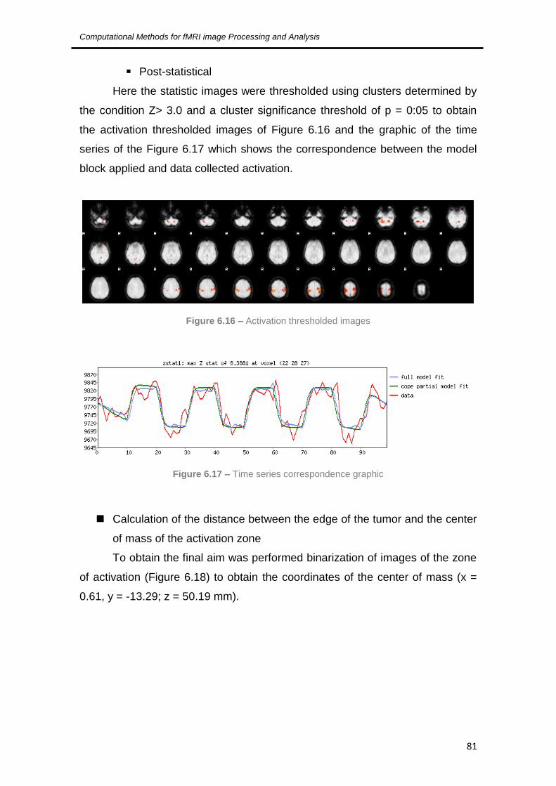
Computational Methods for fMRI image Processing and Analysis
81
Post-statistical
Here the statistic images were thresholded using clusters determined by
the condition Z> 3.0 and a cluster significance threshold of p = 0:05 to obtain
the activation thresholded images of Figure 6.16 and the graphic of the time
series of the Figure 6.17 which shows the correspondence between the model
block applied and data collected activation.
Figure 6.16 – Activation thresholded images
Figure 6.17 – Time series correspondence graphic
Calculation of the distance between the edge of the tumor and the center
of mass of the activation zone
To obtain the final aim was performed binarization of images of the zone
of activation (Figure 6.18) to obtain the coordinates of the center of mass (x =
0.61, y = -13.29; z = 50.19 mm).

Chapter 7 – Implementation, Results and Discussion
82
Figure 6.18 – Binarized activation area
Finally distancemap function was used to calculate all the distances
between the point coordinates of the center of mass and the points on the
periphery of the tumor, obtaining the minimum distance d = 30.47 mm.
6.3.2. MATLAB
The work developed in MATLAB was divided into three phases: a first
phase where data were treated in their raw form, in DICOM format, for semi-
automatic segmentation of the tumour; a second stage, using the SPM, for the
treatment of the functional data, in NIfTI format, for obtaining the areas of
activation and obtaining the coordinates of its centre of mass; and a third phase
with the conjugation of the area corresponding to the tumour with the area of
activation obtained, which allowed to obtain the coordinates of tumour closest
point to the centre of mass for the final calculation of the distance between
these two points.
Phase 1
At this stage two algorithms have been developed for segmentation of
tumour in anatomical images, both using the region growing method, one for the
2D segmentation and another 3D segmentation.
This method will group the pixels into regions according to the similarity
between neighbour pixels. After defining the initial seed pixel, the algorithm will
check which neighbour pixels satisfy the similarity criteria established (such as

Computational Methods for fMRI image Processing and Analysis
83
intensity values) and will group them to create a region of interest. The process
stops when the difference between the average values of the region and the
new pixel exceeds a certain threshold set [38].
In figure 6.19 we can see the 2D segmentation result, initially developed
for checking the correct selection of the region corresponding to the tumour.
Figure 6.19 – 2D segmentation results
Then the algorithm was developed for the 3D segmentation of the
tumour. This algorithm was also based on the Region Growing method. Here,
the initial seed was selected on the preview data in 3D (Figure 6.20) to obtain
the coordinates of a central pixel of the tumour and the result can be seen in
Figure 6.21.
Figure 6.20 – 3D preview of the initial data

Chapter 7 – Implementation, Results and Discussion
84
Figure 6.21 – 3D tumour segmentation result
Phase 2
At this stage a first-level analysis to functional data was made. This
analysis began with the pre-processing of functional data where they were
subjected to the following steps: realign of the time-series images through a
routine of SPM that uses a least squares approach and a 6 parameter spatial
transformation. In this case, the first image of the series is the one that will be
used as reference. Simultaneously, this routine will also remove motion
artefacts inherent to this type of exams; smoothing of the data with a [8x8x8]
Gaussian kernel in order to remove any noise present in the image volume [40].
After this pre-processing the first level functional analysis was done using
a routine specific from SPM with the same experimental block design of Figure
6.13, and whose matrix applied this analysis is shown in Figure 6.22.

Computational Methods for fMRI image Processing and Analysis
85
Figure 6.22 – Design matrix for the SPM statistical analysis
The final results of this analysis can be seen in Figure 6.23 where it is
possible to see the table of estimated values for the formation of clusters and
the location of areas of activation and Figures 6.24 and 6.25 is possible to see
the difference in intensities in different areas of the brain.
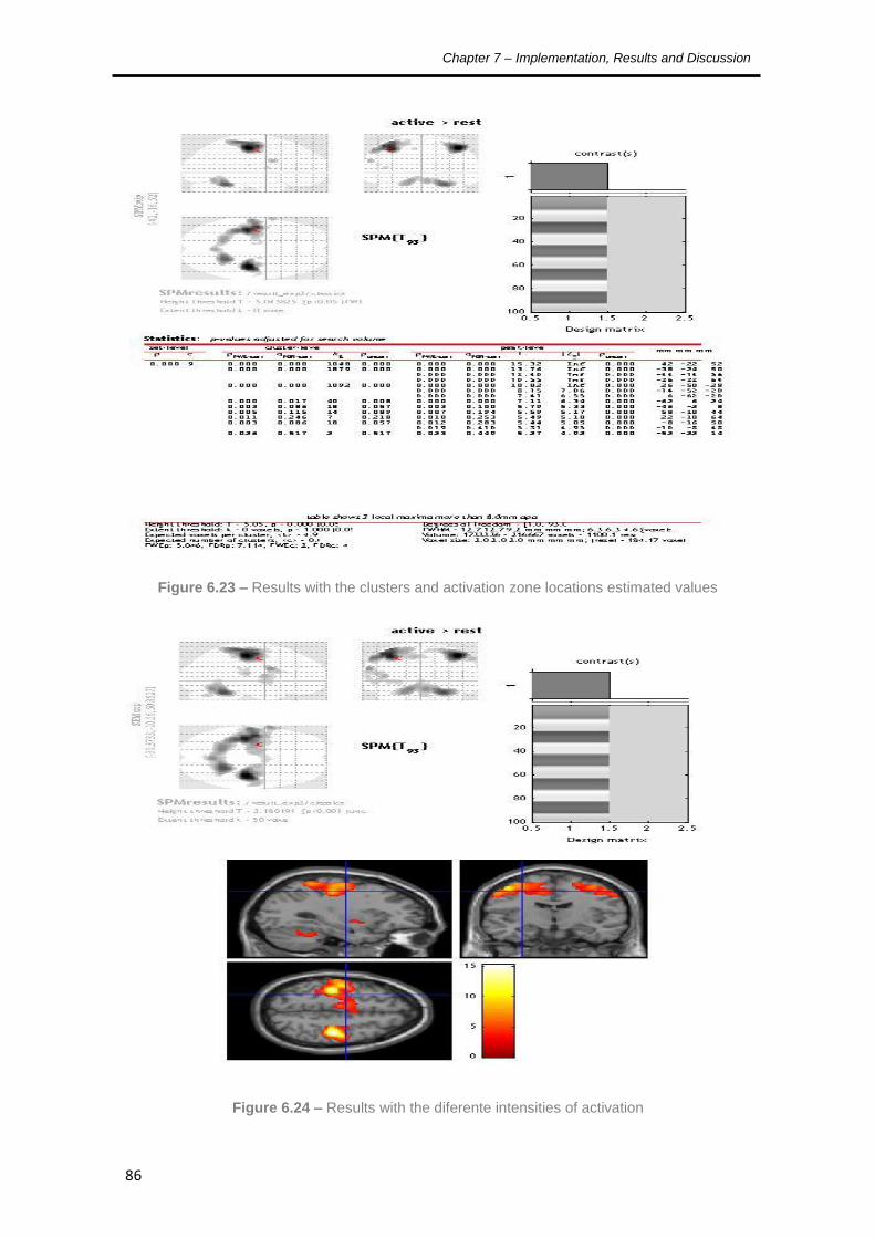
Chapter 7 – Implementation, Results and Discussion
86
Figure 6.23 – Results with the clusters and activation zone locations estimated values
Figure 6.24 – Results with the diferente intensities of activation

Computational Methods for fMRI image Processing and Analysis
87
Figure 6.25 – 3D visualization of the location of the activation areas
After obtaining this statistical analysis, with the identification of the
activation areas, region of interest was created corresponding to the location of
these brain activations through the tool MarsBaR (Marseille Boite à Région
d'Intéret) SPM, obtaining the results visible in Figures 6.26 and 6.27 in 3D [47].
Figure 6.26 – Region of interest of the activation areas

Chapter 7 – Implementation, Results and Discussion
88
Figure 6.27 – 3D representation of the regions of interest
From Figure 6.26 it was possible to obtain information relating to the area
of activation as the location of its centre of mass with the coordinates x = -17.5,
y = -15.5, z = 42.1 mm.
Then using the same tool and the segmented tumour on the first stage
was also obtained the region of interest corresponding to the tumour seen in
Figure 6.28.
Figure 6.28 – Region of interest of the tumour area

Computational Methods for fMRI image Processing and Analysis
89
Phase 3
In this last phase, after combining the tumour region of interest with the
coordinates of the centre of mass been we obtained ,with the same tool, the
closest point between the tumour and centre of mass point, with the coordinates
x = -31.8; y = -15.2, z = 35.3.
With these two sets of coordinates is possible to obtain the distance
between them by use of the equation 6.1 to calculate the Euclidean distance:
√
Equation 6.1 – Euclidean distance
Thus was obtained a distance d = 15.83 mm.
6.4. Discussion
As can be seen there is a large discrepancy between the values obtained
with the two different software’s.
This may be due mainly to computation differences between the two
software’s and the different approaches made, considering the limitations of
each.
In the case of FSL, as it is a specific software for statistical analysis of
fMRI tests, it presents more limitations in the handling of anatomical images,
that is, as the segmentation of the tumour process was based on a manual
study of the tumour coordinates, it is possible that this has led to an imprecise
segmentation, which in turn may partly explain this large difference in the
distance values.
In the case of MATLAB, as this is a more powerful calculation tool it
enabled the semi-automatic segmentation of the tumour, that is, less subject to
errors of a user and as the SPM could use the results of this segmentation and
conjugated them with statistical analysis of the data, is likely to have obtained a
value for the distance more precise, despite the manual character of the final
calculation.

Chapter 7 – Implementation, Results and Discussion
90
Yet it is not possible to determine with certainty which value is more
accurate, it would be necessary to obtain the opinion of a medical expert and
analyse the results in every step of the process based on his professional
experience.
It would also be useful to test these approaches in other data sets and
observe the possible outcomes.

91
7. Conclusions and Future perspectives

Chapter 8 – Conclusions and Future perspectives
92
For the study made for the measuring the distance between the edge of
a tumour and the centre of mass of an activation area several reviews were
carried out, from the brain anatomy and its pathologies, to the physics inherent
in acquisition techniques of MR and fMR images, to the processing techniques
of this kind of images that were the basis for the practical implementation of this
work.
This study used two software’s: FSL and MATLAB, with the testing of two
different implementation approaches, to obtain the results.
The final results showed first that the two software’s work very differently,
and that the analysis of fMRI data, while being a statistical based study,
requires a more complex analysis to better understand the discrepancy of
values; and in second place that the segmentation techniques used require
further refinement and validation of accuracy by a medical specialist. However,
although this evaluation is not possible, one can say that the work is promising
if continued its development, since the study of these distances can be used for
the diagnosis and possible treatment of brain tumours without affecting the
functional areas.
Two perspectives for future research would be the selection of one of the
software’s to work exclusively for testing more data volumes with medical
validation and possible automation of the computational process.

93
References
[1] S. V. Madihally, Principles of Biomedical Engineering, Norwood: Artech House,
2010.
[2] J. L. Prince and J. Links, Medical Imaging Signals and Systems, Prentice Hall,
2005.
[3] J. T. Hansen, Netter's Clinical Anatomy, Philadelphia: Saunders, Elsevier, 2010.
[4] V. S. Ramachandran, Encyclopedia of the Human Brain, Academic Press, 2002.
[5] B. Cummings, “Chapter 12: Functional Areas of the Cerebral Cortex,” Austin Peay
State University, [Online]. Available: http://www.apsu.edu/. [Accessed 10 January
2013].
[6] R. Seeley, T. Stephens and P. Tate, Anatomia & Fisiologia, 6ª ed., McGraw-Hill
Companies, 2003.
[7] B. Greenstein and A. Greenstein, Color Atlas of Neuroscience: Neuroanatomy and
Neurophysiology, Thieme, 2000.
[8] A. C. Poinier, “WebMD,” Healthwise Staff, 09 November 2010. [Online]. Available:
http://www.webmd.com.
[9] Cancer Research UK, “Brain, other CNS and intracranial tumours incidence
statistics,” 28 March 2013. [Online]. Available:
http://www.cancerresearchuk.org/cancer-
info/cancerstats/types/brain/incidence/#Distribution. [Accessed 17 April 2013].
[10] L. Tonarelli, “Magnetic Resonance Imaging of Brain Tumor,” [Online]. Available:
http://www.cewebsource.com/coursePDFs/MRIBrainTumor.pdf. [Accessed 12
September 2012].
[11] M. Bethesda, “Adult Brain Tumors Treatment,” 2013. [Online]. Available:
http://cancer.gov/cancertopics/pdq/treatment/adultbrain/HealthProfessional.
[Accessed 14 April 2013].
[12] L. Landini, V. Positano and M. Santarelli, Advanced Image Processing in Magnetic
Resonance Imaging, Boca Raton: Taylor & Francis Group, LLC, 2005.
[13] R. Khandpur, Biomedical Instrumentation: Technology and Applications, McGraw-
Hill Professional, 2004.
[14] M. Kutz, Biomedical Engineering and Desing Handbook Volume 2: Applications,

Chapter 8 – Conclusions and Future perspectives
94
McGraw-Hill Companies, 2009.
[15] J. D. Bronzino, The Biomedical Engineering HandBook, 2º ed., CRC Press, LLC,
2002.
[16] M. C. F. N. S. Hage and M. Iwasaki, “Imagem por ressonância magnética:
princípios básicos,” Ciência Rural, vol. 39, no. 4, pp. 1287-1295, 2009.
[17] A. A. Mazzola, “Ressonância Magnética: princípios de formação da imagem e
aplicações em imagem funcional,” Revista Brasileira de Física Médica, vol. 3, no.
1, pp. 117-129, 2009.
[18] R. K. Hobbie and B. J. Roth, Intermediate Physics for Medicine and Biology,
Springer, 2007.
[19] J. D. Enderle, S. M. Blanchard and J. D. Bronzino, Introduction to Biomedical
Engineering, Elsevier Academic Press, 2005.
[20] M. T. Vlaardingerbroek and J. A. Boer, Magnetic Resonance Imaging – Theory
and Practice, 3º ed., Berlin: Springer, 2003.
[21] R. A. Pooley, “AAPM/RSNA Physics Tutorial for Residents: Fundamental Physics
of MR Imaging,” Radiographics, vol. 25, no. 4, pp. 1087-1099, 2005.
[22] R. B. Buxton, Introduction to Functional Magnetic Resonance Imaging - Principles
and Techniques, 2º ed., Cambridge University Press, 2009.
[23] M. A. Brown and R. C. Semelka, MRI : basic principles and applications, 3º ed.,
New Jersey: John Wiley and Sons, 2003.
[24] S. H. Faro and F. B. Mohamed, BOLD fMRI - A Guide to Functional Imaging for
Neuroscientists, New York: Springer, 2010.
[25] S. Ogawa, T. M. Lee, A. R. Kay and D. W. Tank, “Brain magnetic resonance
imaging with contrast dependent on blood oxygenation,” Proceedings of the
National Academy of Sciences, vol. 87, pp. 9868-9872, 1990.
[26] P. Figueiredo, “O cérebro humano em actividade: investigação imagiológica por
ressonância magnética funcional,” Gazeta de Física, vol. 31, no. 1/2, pp. 8-12,
2008.
[27] L. Pauling and C. D. Coryell, “The magnetic properties and structure of
hemoglobine, oxyhemoglobine and carbonmonoxyhemoglobine,” Proceedings of
the National Academy of Sciences, vol. 22, no. 4, pp. 210-216, 1936.
[28] P. Bogorodzki and J. Rogowska, “Structural Group Classification Technique based
on Regional fMRI BOLD Response,” IEEE Transactions on Medical Imaging, vol.
24, no. 3, pp. 389-398, 2005.

Computational Methods for fMRI image Processing and Analysis
95
[29] P. Kenning, H. Plassmann and D. Ahlert, “Applications of functional magnetic
resonance imaging for market research,” Qualitative Market Research: An
International Journal, vol. 10, no. 2, pp. 135-152, 2007.
[30] R. Savoy, “Functional Magnetic Resonance Imaging (fMRI),” in Encyclopedia of
the Human Brain Vol.2, Elsevier Science, 2002, pp. 327-350.
[31] P. M. Matthews and P. Jezzard, “Functional magnetic resonance imaging,” Journal
of Neurology, Neurosurgery and Psychiatry, vol. 75, no. 1, pp. 6-12, 2004.
[32] E. Amaro Jr. and G. J. Barker, Study design in fMRI: Basic principles, Brain and
Cognition, Elsevier, 2006.
[33] J. Jorge, W. Zwaag and P. Figueiredo, “EEG-fMRI integration for the study of
human brain,” NeuroImage, vol. accepted, 2013.
[34] M. Smith, “Functional Magnetic Resonance Imaging (fMRI) in Brain Tumour
Patients,” European Association of NeuroOncology Magazine, vol. 12, no. 3, pp.
123-128, 2012.
[35] P. Brandão and A. M. Reis, “Erro médico em imagiologia,” Acta Médica
Portuguesa, vol. 19, pp. 235-238, 2006.
[36] E. Formisano, F. Salle and R. Goebel, “Fundamentals of Data Analysis Methods in
Functional MRI,” in Advanced Image Processing in Magnetic Resonance Imaging,
Taylor & Francis Group, LLC, 2005, pp. 481-500.
[37] M. Jenkinson and S. Smith, “The Role of Registration in Functional Magnetic,” in
Medical Image Registration, CRC Press LLC, 2001, pp. 183-198.
[38] R. Gonzales and R. Woods, Digital Image Processing, 2º ed., Prentice Hall, 2002.
[39] R. Maini and H. Aggarwal, “A comprehensive review of image enhancement
techniques,” Journal of Computing, vol. 2, no. 3, pp. 8-13, 2010.
[40] Guillaume, “SPM - Statistical Parametric Mapping,” Wellcome Trust Centre for
Neuroimaging, 24 Junho 2013. [Online]. Available: http://www.fil.ion.ucl.uk/spm.
[41] S. Smith, “FSL - FslWiki,” Analysis Group, 11 06 2013. [Online]. Available:
http://fsl.fmrib.ox.ac.uk/fsl.
[42] M. Jenkinson, P. Bannister and J. M. a. S. S. M. Brady, “Improved Optimisation for
the Robust and Accurate Linear Registration and Motion Correction of Brain
Images,” NeuroImage, vol. 17, no. 2, pp. 825-841, 2002.
[43] S. M. Smith, “Fast robust automated brain extraction,” Human Brain Mapping, vol.
17, no. 3, pp. 143-155, 2002.
[44] S. Smith and J. Brady, “SUSAN - a new approach to low level image processing,”

Chapter 8 – Conclusions and Future perspectives
96
International Journal of Computer Vision, vol. 23, no. 1, pp. 45-78, 1997.
[45] Y. Zhang, M. Brady and S. Smith, “Segmentation of brain MR images through a
hidden Markov random field model and the expectation-maximization algorithm,”
IEEE Trans Med Imag, vol. 20, no. 1, pp. 45-57, 2001.
[46] M. Woolrich, B. Ripley and J. a. S. S. Brady, “Temporal Autocorrelation in
Univariate Linear Modelling of FMRI Data,” NeuroImage, vol. 14, no. 6, pp. 1370-
1386, 2001.
[47] M. Brett, J. L. Anton, R. Valabregue and J. B. Poline, “Region of interest analysis
using an SPM toolbox,” NeuroImage, vol. 16, no. 2, 2002.