Computational Logic

The Prolog Programming Language

1

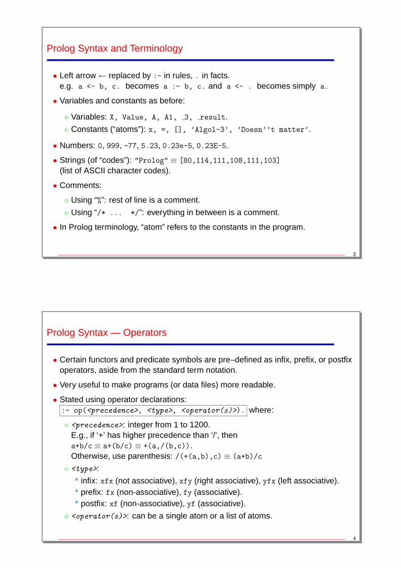
Prolog

• A practical logic language based on the logic programming paradigm.

• Main differences with “pure” logic programming:

� more control on the execution flow,� depth-first search rule, left-to-right control rule,� some pre-defined predicates are not declarative (generally for efficiency),� higher-order and meta-logical capabilities,� no occur check in unification; but often regular (i.e., infinite) trees supported.

• Advantages:

� it can be compiled into fast and efficient code,� more expressive power,� industry standard (ISO-Prolog),� mature implementations with modules, graphical environments, interfaces, ...

• Drawbacks: incompleteness (due to depth-first search rule),possible unsoundness (if no occur check and regular trees not supported).

2

Prolog Syntax and Terminology

• Left arrow← replaced by :- in rules, . in facts.e.g. a <- b, c. becomes a :- b, c. and a <- . becomes simply a.

• Variables and constants as before:

� Variables: X, Value, A, A1, 3, result.

� Constants (“atoms”): x, =, [], ’Algol-3’, ’Doesn’’t matter’.

• Numbers: 0, 999, -77, 5.23, 0.23e-5, 0.23E-5.

• Strings (of “codes”): "Prolog" ≡ [80,114,111,108,111,103]

(list of ASCII character codes).

• Comments:

� Using “%”: rest of line is a comment.

� Using “/* ... */”: everything in between is a comment.

• In Prolog terminology, “atom” refers to the constants in the program.

3

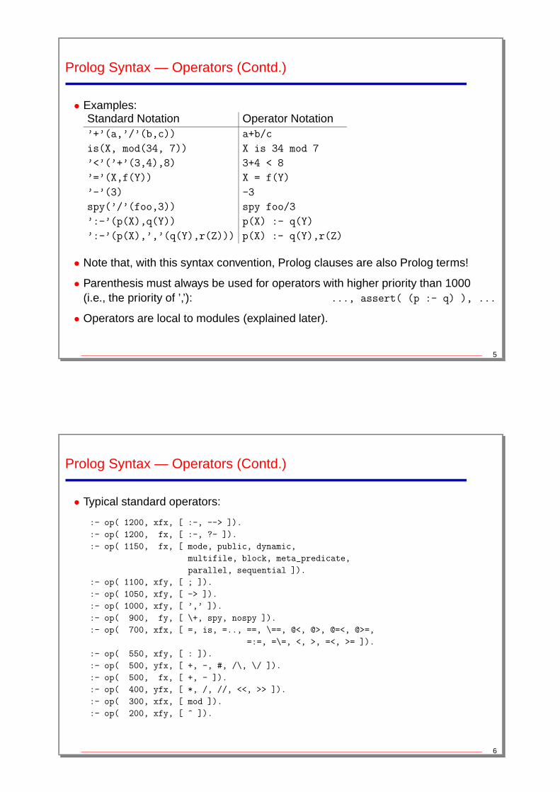
Prolog Syntax — Operators

• Certain functors and predicate symbols are pre–defined as infix, prefix, or postfixoperators, aside from the standard term notation.

• Very useful to make programs (or data files) more readable.

• Stated using operator declarations::- op(<precedence>, <type>, <operator(s)>). where:

� <precedence>: integer from 1 to 1200.E.g., if ‘+’ has higher precedence than ‘/’, thena+b/c ≡ a+(b/c) ≡ +(a,/(b,c)).Otherwise, use parenthesis: /(+(a,b),c) ≡ (a+b)/c

� <type>:

* infix: xfx (not associative), xfy (right associative), yfx (left associative).* prefix: fx (non-associative), fy (associative).* postfix: xf (non-associative), yf (associative).

� <operator(s)>: can be a single atom or a list of atoms.

4

Prolog Syntax — Operators (Contd.)

• Examples:Standard Notation Operator Notation’+’(a,’/’(b,c)) a+b/c

is(X, mod(34, 7)) X is 34 mod 7

’<’(’+’(3,4),8) 3+4 < 8

’=’(X,f(Y)) X = f(Y)

’-’(3) -3

spy(’/’(foo,3)) spy foo/3

’:-’(p(X),q(Y)) p(X) :- q(Y)

’:-’(p(X),’,’(q(Y),r(Z))) p(X) :- q(Y),r(Z)

• Note that, with this syntax convention, Prolog clauses are also Prolog terms!

• Parenthesis must always be used for operators with higher priority than 1000(i.e., the priority of ’,’): ..., assert( (p :- q) ), ...

• Operators are local to modules (explained later).

5

Prolog Syntax — Operators (Contd.)

• Typical standard operators:

:- op( 1200, xfx, [ :-, --> ]).

:- op( 1200, fx, [ :-, ?- ]).

:- op( 1150, fx, [ mode, public, dynamic,

multifile, block, meta_predicate,

parallel, sequential ]).

:- op( 1100, xfy, [ ; ]).

:- op( 1050, xfy, [ -> ]).

:- op( 1000, xfy, [ ’,’ ]).

:- op( 900, fy, [ \+, spy, nospy ]).

:- op( 700, xfx, [ =, is, =.., ==, \==, @<, @>, @=<, @>=,

=:=, =\=, <, >, =<, >= ]).

:- op( 550, xfy, [ : ]).

:- op( 500, yfx, [ +, -, #, /\, \/ ]).

:- op( 500, fx, [ +, - ]).

:- op( 400, yfx, [ *, /, //, <<, >> ]).

:- op( 300, xfx, [ mod ]).

:- op( 200, xfy, [ ^ ]).

6

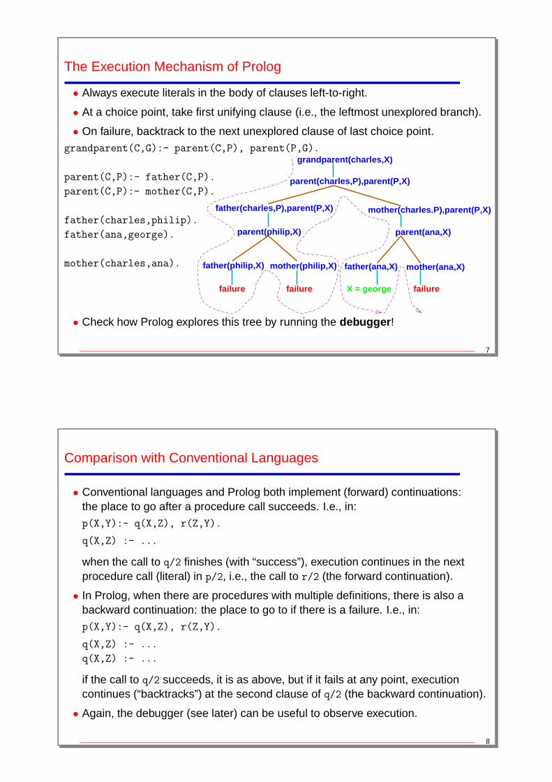
The Execution Mechanism of Prolog

• Always execute literals in the body of clauses left-to-right.

• At a choice point, take first unifying clause (i.e., the leftmost unexplored branch).

• On failure, backtrack to the next unexplored clause of last choice point.grandparent(C,G):- parent(C,P), parent(P,G).

parent(C,P):- father(C,P).

parent(C,P):- mother(C,P).

father(charles,philip).

father(ana,george).

mother(charles,ana).

grandparent(charles,X)

parent(charles,P),parent(P,X)

mother(charles.P),parent(P,X)

parent(ana,X)

mother(ana,X)father(ana,X)mother(philip,X)father(philip,X)

parent(philip,X)

father(charles,P),parent(P,X)

failure failure failureX = george

• Check how Prolog explores this tree by running the debugger!

7

Comparison with Conventional Languages

• Conventional languages and Prolog both implement (forward) continuations:the place to go after a procedure call succeeds. I.e., in:

p(X,Y):- q(X,Z), r(Z,Y).

q(X,Z) :- ...

when the call to q/2 finishes (with “success”), execution continues in the nextprocedure call (literal) in p/2, i.e., the call to r/2 (the forward continuation).

• In Prolog, when there are procedures with multiple definitions, there is also abackward continuation: the place to go to if there is a failure. I.e., in:

p(X,Y):- q(X,Z), r(Z,Y).

q(X,Z) :- ...

q(X,Z) :- ...

if the call to q/2 succeeds, it is as above, but if it fails at any point, executioncontinues (“backtracks”) at the second clause of q/2 (the backward continuation).

• Again, the debugger (see later) can be useful to observe execution.

8

Control of Search in Prolog

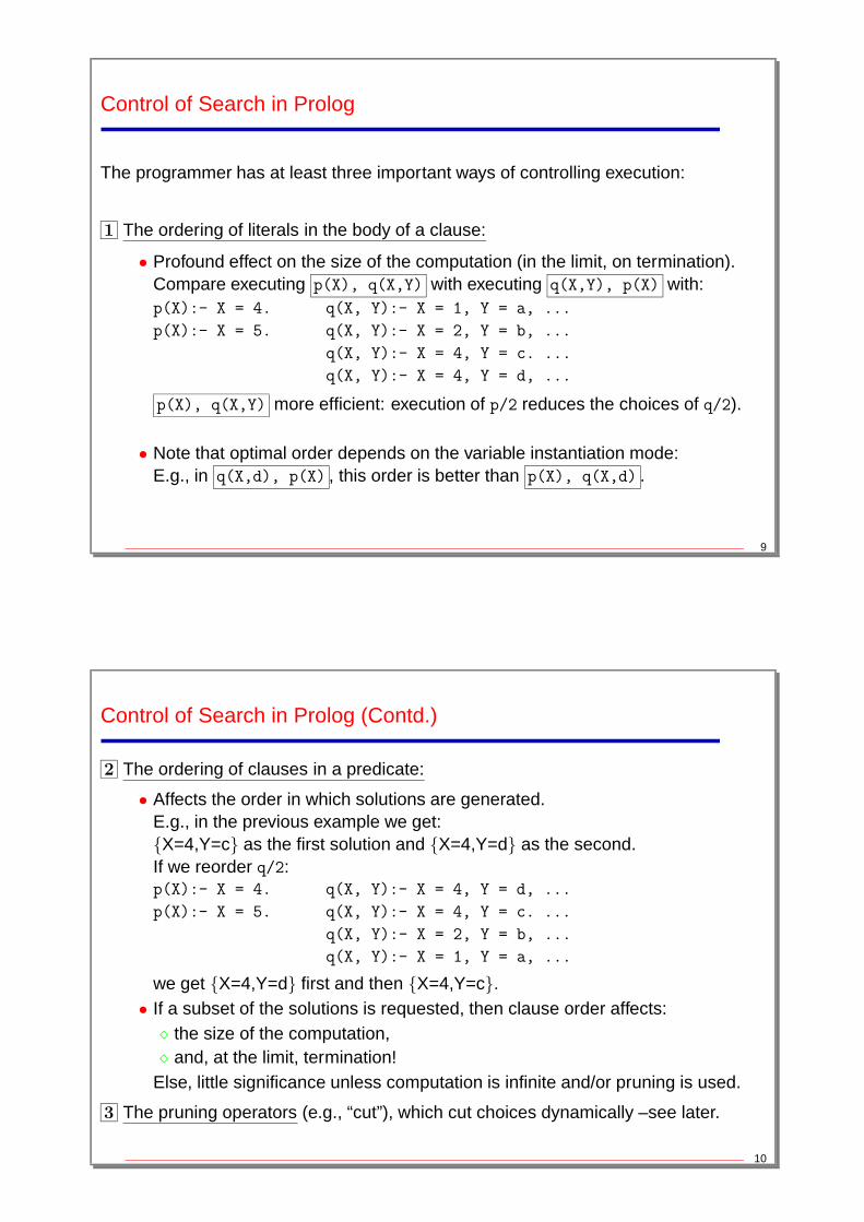
The programmer has at least three important ways of controlling execution:

1 The ordering of literals in the body of a clause:

• Profound effect on the size of the computation (in the limit, on termination).Compare executing p(X), q(X,Y) with executing q(X,Y), p(X) with:p(X):- X = 4. q(X, Y):- X = 1, Y = a, ...

p(X):- X = 5. q(X, Y):- X = 2, Y = b, ...

q(X, Y):- X = 4, Y = c. ...

q(X, Y):- X = 4, Y = d, ...

p(X), q(X,Y) more efficient: execution of p/2 reduces the choices of q/2).

• Note that optimal order depends on the variable instantiation mode:E.g., in q(X,d), p(X) , this order is better than p(X), q(X,d) .

9

Control of Search in Prolog (Contd.)

2 The ordering of clauses in a predicate:

• Affects the order in which solutions are generated.E.g., in the previous example we get:{X=4,Y=c} as the first solution and {X=4,Y=d} as the second.If we reorder q/2:p(X):- X = 4. q(X, Y):- X = 4, Y = d, ...

p(X):- X = 5. q(X, Y):- X = 4, Y = c. ...

q(X, Y):- X = 2, Y = b, ...

q(X, Y):- X = 1, Y = a, ...

we get {X=4,Y=d} first and then {X=4,Y=c}.• If a subset of the solutions is requested, then clause order affects:� the size of the computation,� and, at the limit, termination!

Else, little significance unless computation is infinite and/or pruning is used.

3 The pruning operators (e.g., “cut”), which cut choices dynamically –see later.

10

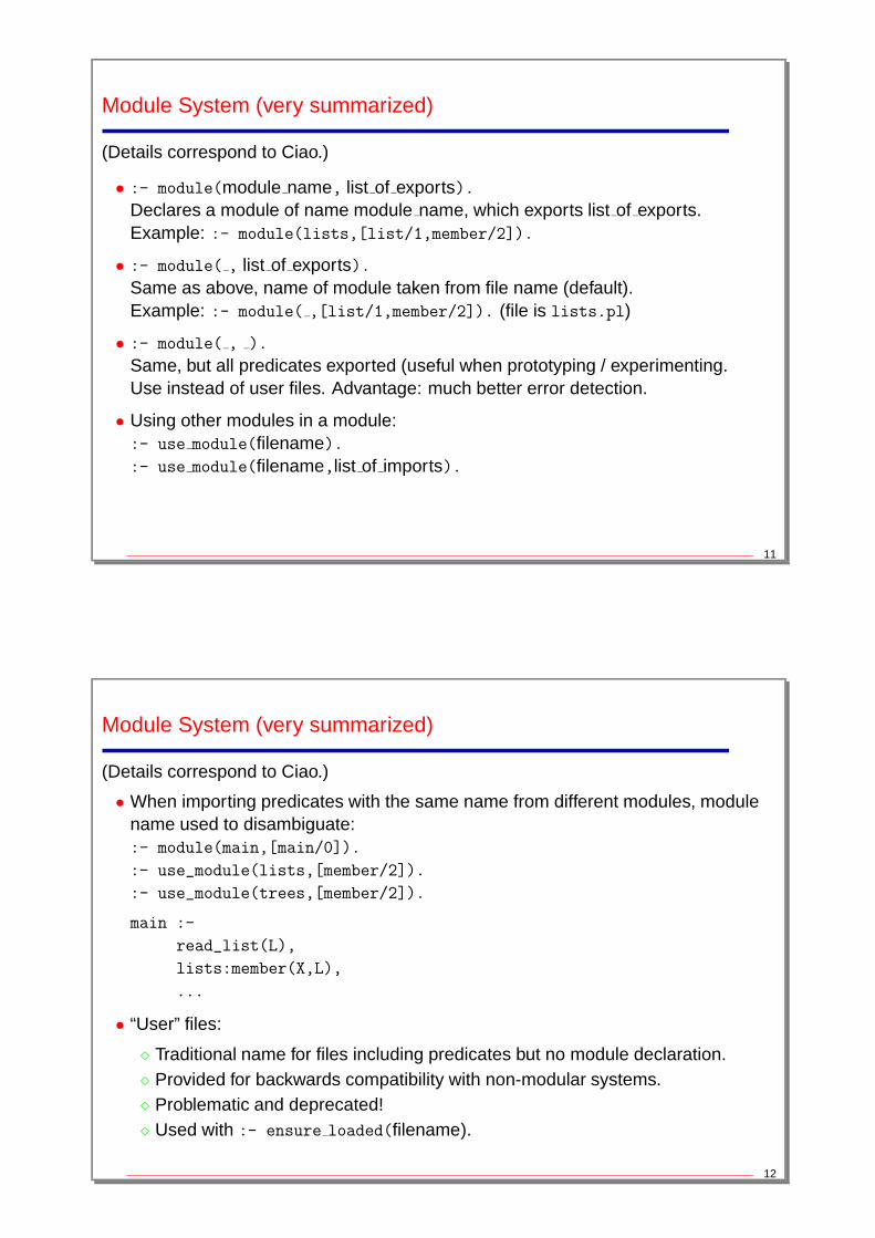
Module System (very summarized)

(Details correspond to Ciao.)

• :- module(module name, list of exports).Declares a module of name module name, which exports list of exports.Example: :- module(lists,[list/1,member/2]).

• :- module( , list of exports).Same as above, name of module taken from file name (default).Example: :- module( ,[list/1,member/2]). (file is lists.pl)

• :- module( , ).

Same, but all predicates exported (useful when prototyping / experimenting.Use instead of user files. Advantage: much better error detection.

• Using other modules in a module::- use module(filename).:- use module(filename,list of imports).

11

Module System (very summarized)

(Details correspond to Ciao.)

• When importing predicates with the same name from different modules, modulename used to disambiguate::- module(main,[main/0]).

:- use_module(lists,[member/2]).

:- use_module(trees,[member/2]).

main :-

read_list(L),

lists:member(X,L),

...

• “User” files:

� Traditional name for files including predicates but no module declaration.� Provided for backwards compatibility with non-modular systems.� Problematic and deprecated!� Used with :- ensure loaded(filename).

12

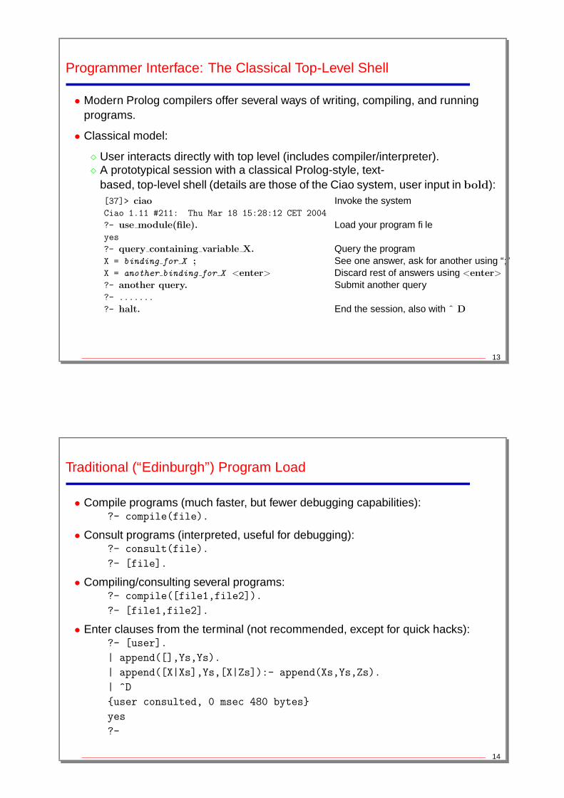
Programmer Interface: The Classical Top-Level Shell

• Modern Prolog compilers offer several ways of writing, compiling, and runningprograms.

• Classical model:

� User interacts directly with top level (includes compiler/interpreter).� A prototypical session with a classical Prolog-style, text-

based, top-level shell (details are those of the Ciao system, user input in bold):[37]> ciao Invoke the systemCiao 1.11 #211: Thu Mar 18 15:28:12 CET 2004

?- use module(file). Load your program fileyes

?- query containing variable X. Query the programX = binding for X ; See one answer, ask for another using “;”X = another binding for X <enter> Discard rest of answers using <enter>

?- another query. Submit another query?- .......

?- halt. End the session, also with ˆ D

13

Traditional (“Edinburgh”) Program Load

• Compile programs (much faster, but fewer debugging capabilities):?- compile(file).

• Consult programs (interpreted, useful for debugging):?- consult(file).

?- [file].

• Compiling/consulting several programs:?- compile([file1,file2]).

?- [file1,file2].

• Enter clauses from the terminal (not recommended, except for quick hacks):?- [user].

| append([],Ys,Ys).

| append([X|Xs],Ys,[X|Zs]):- append(Xs,Ys,Zs).

| ^D

{user consulted, 0 msec 480 bytes}

yes

?-

14

Ciao Program Load

• Traditional (“Edinburgh”) program load commands can be used.

• More modern primitives available which take into account module system.Same commands used as in the code inside a module:

� use module/1 – for loading modules.

� ensure loaded/1 – for loading user files.

� use package/1 – for loading packages (see later).

• In summary, top-level behaves essentially like a module.

• In practice, done automatically within graphical environment:

� Open source file in graphical environment.

� Load (typing C-c l or using menu).

15

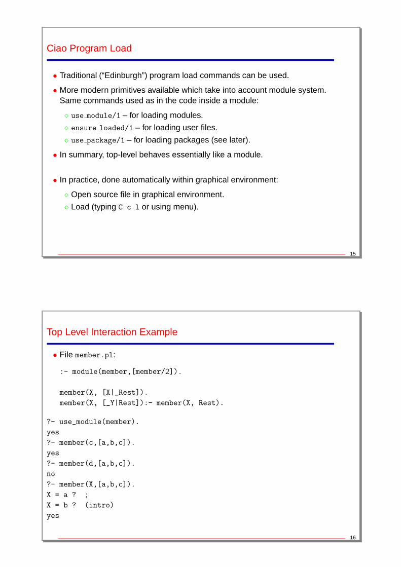
Top Level Interaction Example

• File member.pl:

:- module(member,[member/2]).

member(X, [X|_Rest]).

member(X, [_Y|Rest]):- member(X, Rest).

?- use_module(member).

yes

?- member(c,[a,b,c]).

yes

?- member(d,[a,b,c]).

no

?- member(X,[a,b,c]).

X = a ? ;

X = b ? (intro)

yes

16

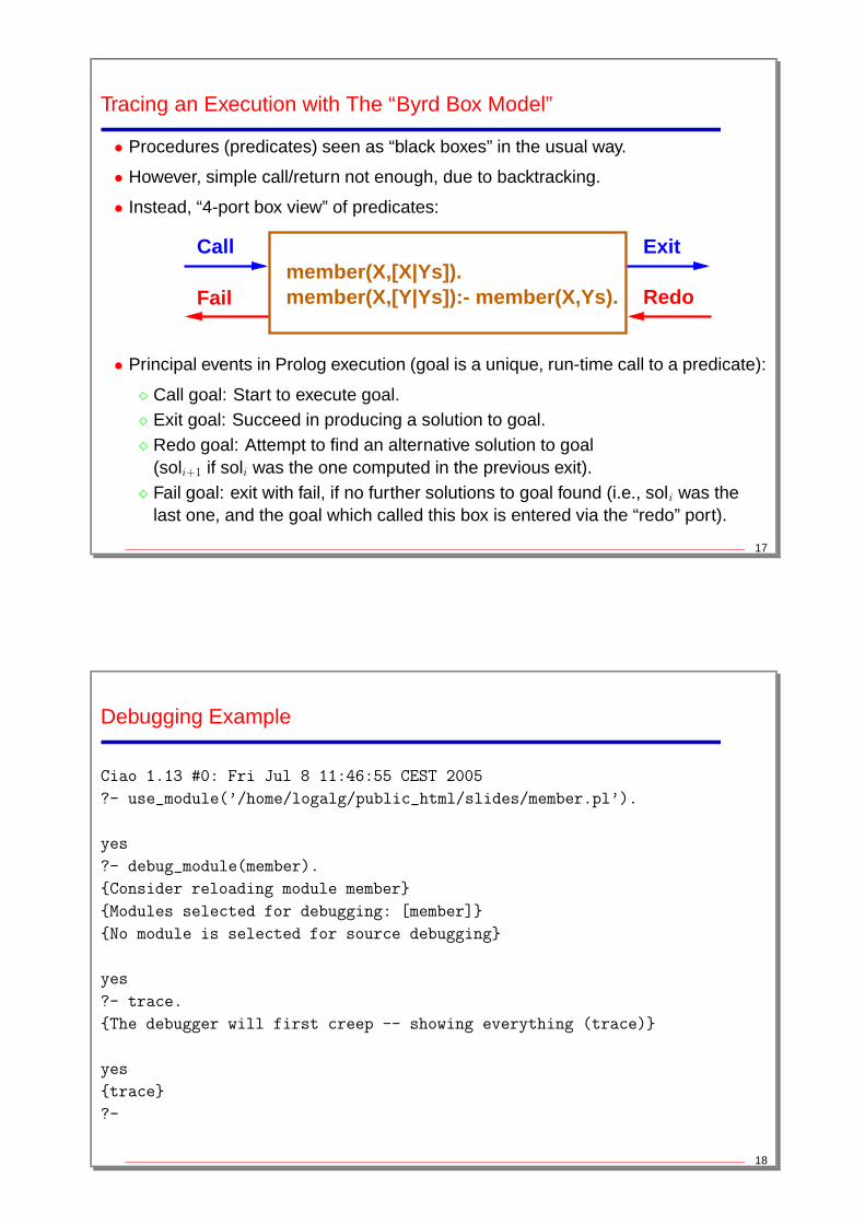
Tracing an Execution with The “Byrd Box Model”

• Procedures (predicates) seen as “black boxes” in the usual way.

• However, simple call/return not enough, due to backtracking.

• Instead, “4-port box view” of predicates:

RedoFail

Call Exit

member(X,[Y|Ys]):- member(X,Ys).member(X,[X|Ys]).

• Principal events in Prolog execution (goal is a unique, run-time call to a predicate):

� Call goal: Start to execute goal.� Exit goal: Succeed in producing a solution to goal.� Redo goal: Attempt to find an alternative solution to goal

(soli+1 if soli was the one computed in the previous exit).� Fail goal: exit with fail, if no further solutions to goal found (i.e., soli was the

last one, and the goal which called this box is entered via the “redo” port).

17

Debugging Example

Ciao 1.13 #0: Fri Jul 8 11:46:55 CEST 2005

?- use_module(’/home/logalg/public_html/slides/member.pl’).

yes

?- debug_module(member).

{Consider reloading module member}

{Modules selected for debugging: [member]}

{No module is selected for source debugging}

yes

?- trace.

{The debugger will first creep -- showing everything (trace)}

yes

{trace}

?-

18

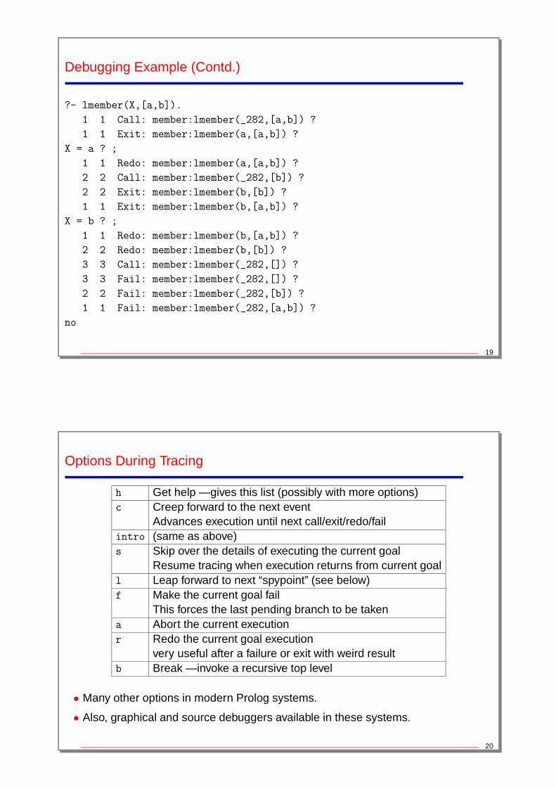
Debugging Example (Contd.)

?- lmember(X,[a,b]).

1 1 Call: member:lmember(_282,[a,b]) ?

1 1 Exit: member:lmember(a,[a,b]) ?

X = a ? ;

1 1 Redo: member:lmember(a,[a,b]) ?

2 2 Call: member:lmember(_282,[b]) ?

2 2 Exit: member:lmember(b,[b]) ?

1 1 Exit: member:lmember(b,[a,b]) ?

X = b ? ;

1 1 Redo: member:lmember(b,[a,b]) ?

2 2 Redo: member:lmember(b,[b]) ?

3 3 Call: member:lmember(_282,[]) ?

3 3 Fail: member:lmember(_282,[]) ?

2 2 Fail: member:lmember(_282,[b]) ?

1 1 Fail: member:lmember(_282,[a,b]) ?

no

19

Options During Tracing

h Get help — gives this list (possibly with more options)c Creep forward to the next event

Advances execution until next call/exit/redo/failintro (same as above)s Skip over the details of executing the current goal

Resume tracing when execution returns from current goall Leap forward to next “spypoint” (see below)f Make the current goal fail

This forces the last pending branch to be takena Abort the current executionr Redo the current goal execution

very useful after a failure or exit with weird resultb Break — invoke a recursive top level

• Many other options in modern Prolog systems.

• Also, graphical and source debuggers available in these systems.

20

Spypoints (and breakpoints)

• ?- spy foo/3.

Place a spypoint on predicate foo of arity 3 – always trace events involving thispredicate.

• ?- nospy foo/3.

Remove the spypoint in foo/3.

• ?- nospyall.

Remove all spypoints.

• In many systems (e.g., Ciao) also breakpoints can be set at particular programpoints within the graphical environment.

21

Debugger Modes

• ?- debug.

Turns debugger on. It will first leap, stopping at spypoints and breakpoints.

• ?- nodebug.

Turns debugger off.

• trace.

The debugger will first creep, as if at a spypoint.

• notrace.

The debugger will leap, stopping at spypoints and breakpoints.

22

Modern Programmer Interfaces

• Modern Prolog compilers offer a variety of facilities for of writing, compiling, andrunning programs.

• For example, the Ciao system offers:

� A graphical environment for editing, compiling, debugging verifying, optimizing,and documenting programs.

� A traditional, command line into an interactive top level.

� A stand-alone compiler (ciaoc).

� Compilation of standalone executables, which can be :

* eager dynamic load* lazy dynamic load* static (without the engine –architecture independent)* fully static/standalone (architecture dependent)

� Prolog scripts (architecture independent)

23

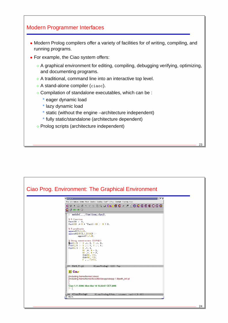
Ciao Prog. Environment: The Graphical Environment

24

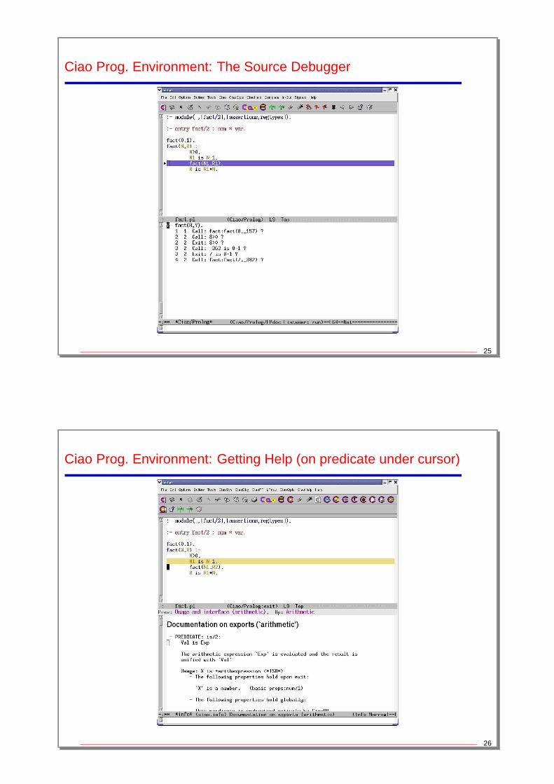
Ciao Prog. Environment: The Source Debugger

25

Ciao Prog. Environment: Getting Help (on predicate under cursor)

26

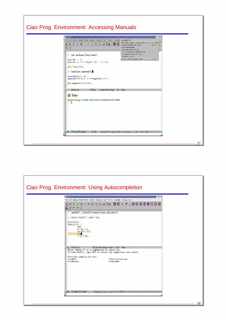
Ciao Prog. Environment: Accessing Manuals

27

Ciao Prog. Environment: Using Autocompletion

28

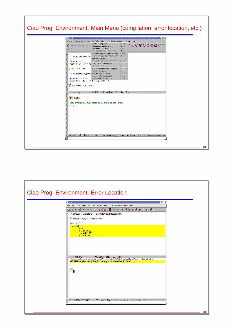
Ciao Prog. Environment: Main Menu (compilation, error location, etc.)

29

Ciao Prog. Environment: Error Location

30

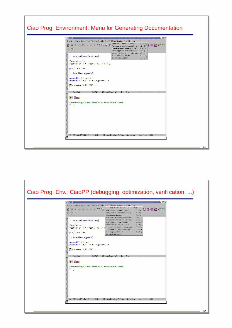
Ciao Prog. Environment: Menu for Generating Documentation

31

Ciao Prog. Env.: CiaoPP (debugging, optimization, verification, ...)

32

Built-in Arithmetic

• Practicality: interface to the underlying CPU arithmetic capabilities.

• These arithmetic operations are not as general as their logical counterparts.

• Interface: evaluator of arithmetic terms.

• The type of arithmetic terms:

� a number is an arithmetic term,

� if f is an n-ary arithmetic functor and X1, ..., Xn are arithmetic terms thenf(X1, ..., Xn) is an arithmetic term.

• Arithmetic functors: +, -, *, / (float quotient), // (integer quotient), mod, and more.Examples:

� (3*X+Y)/Z, correct if when evaluated X, Y and Z are arithmetic terms,otherwise it will raise an error.

� a+3*X raises an error (because a is not an arithmetic term).

33

Built-in Arithmetic (Contd.)

• Built-in arithmetic predicates:

� the usual <, >, =<, >=, =:= (arithmetic equal), =\= (arithmetic not equal), ...Both arguments are evaluated and their results are compared

� Z is X

X (which must be an arithmetic term) is evaluated and result is unified with Z.

• Examples: let X and Y be bound to 3 and 4, respectively, and Z be a free variable:

� Y < X+1, X is Y+1, X =:= Y. fail (the system will backtrack).

� Y < a+1, X is Z+1, X =:= f(a). error (abort).

34

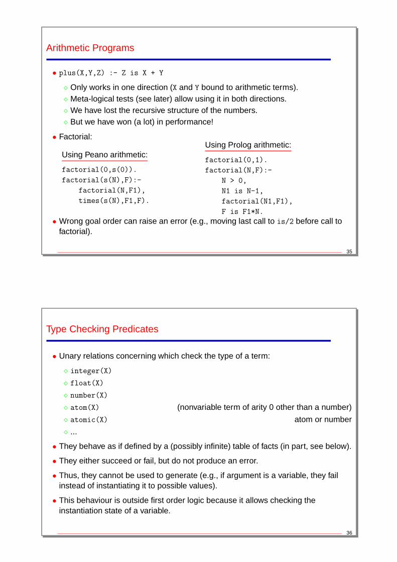
Arithmetic Programs

• plus(X,Y,Z) :- Z is X + Y

� Only works in one direction (X and Y bound to arithmetic terms).� Meta-logical tests (see later) allow using it in both directions.� We have lost the recursive structure of the numbers.� But we have won (a lot) in performance!

• Factorial:

Using Peano arithmetic:

factorial(0,s(0)).

factorial(s(N),F):-

factorial(N,F1),

times(s(N),F1,F).

Using Prolog arithmetic:

factorial(0,1).

factorial(N,F):-

N > 0,

N1 is N-1,

factorial(N1,F1),

F is F1*N.

• Wrong goal order can raise an error (e.g., moving last call to is/2 before call tofactorial).

35

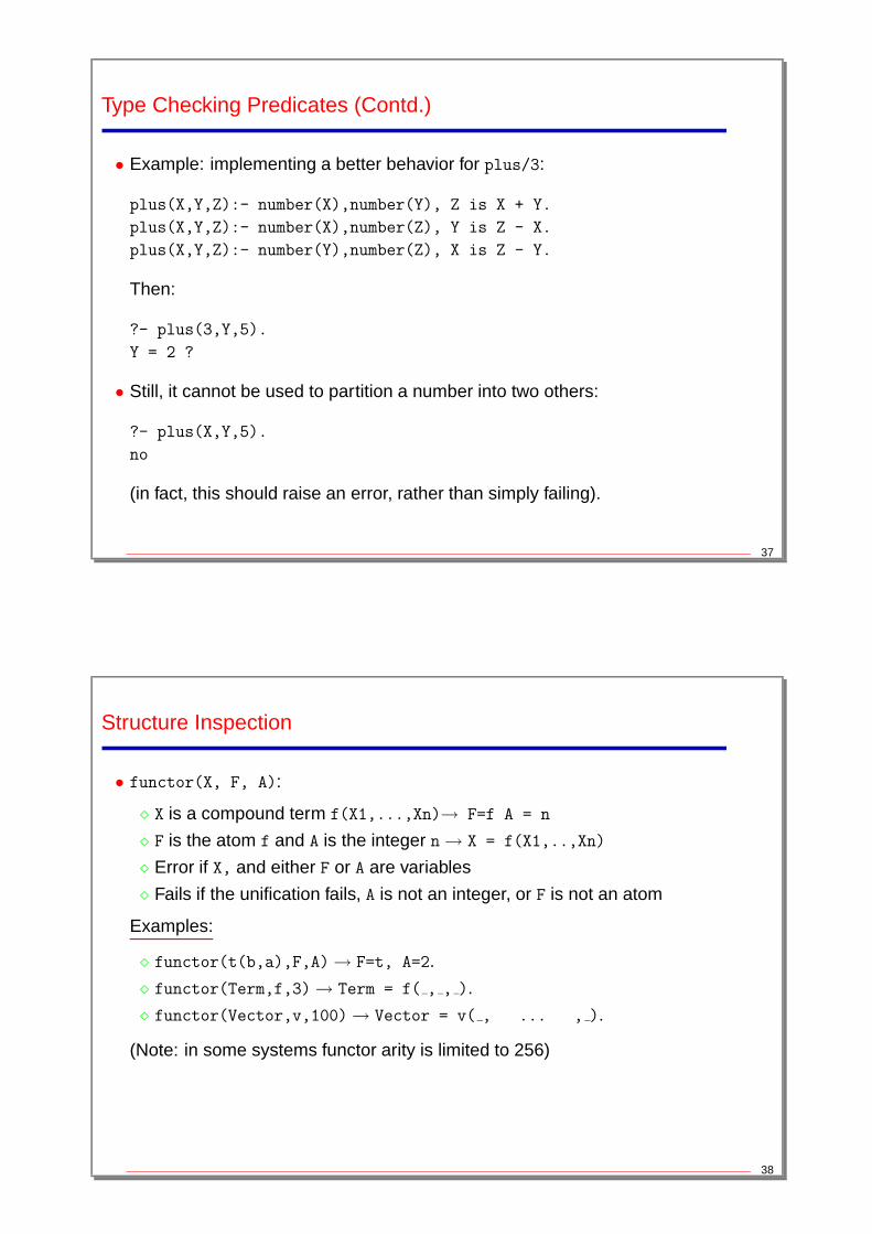
Type Checking Predicates

• Unary relations concerning which check the type of a term:

� integer(X)

� float(X)

� number(X)

� atom(X) (nonvariable term of arity 0 other than a number)

� atomic(X) atom or number

� ...

• They behave as if defined by a (possibly infinite) table of facts (in part, see below).

• They either succeed or fail, but do not produce an error.

• Thus, they cannot be used to generate (e.g., if argument is a variable, they failinstead of instantiating it to possible values).

• This behaviour is outside first order logic because it allows checking theinstantiation state of a variable.

36

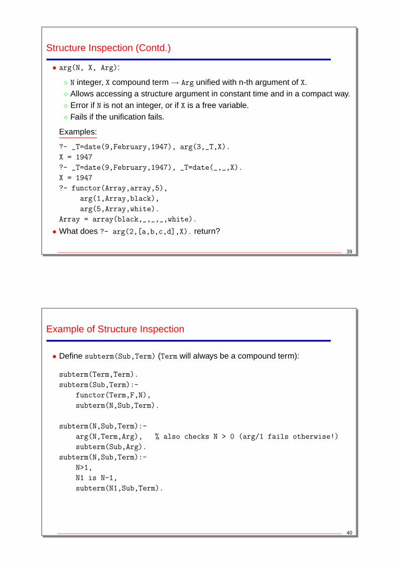
Type Checking Predicates (Contd.)

• Example: implementing a better behavior for plus/3:

plus(X,Y,Z):- number(X),number(Y), Z is X + Y.

plus(X,Y,Z):- number(X),number(Z), Y is Z - X.

plus(X,Y,Z):- number(Y),number(Z), X is Z - Y.

Then:

?- plus(3,Y,5).

Y = 2 ?

• Still, it cannot be used to partition a number into two others:

?- plus(X,Y,5).

no

(in fact, this should raise an error, rather than simply failing).

37

Structure Inspection

• functor(X, F, A):

� X is a compound term f(X1,...,Xn)→ F=f A = n

� F is the atom f and A is the integer n→ X = f(X1,..,Xn)

� Error if X, and either F or A are variables

� Fails if the unification fails, A is not an integer, or F is not an atom

Examples:

� functor(t(b,a),F,A)→ F=t, A=2.

� functor(Term,f,3)→ Term = f( , , ).

� functor(Vector,v,100)→ Vector = v( , ... , ).

(Note: in some systems functor arity is limited to 256)

38

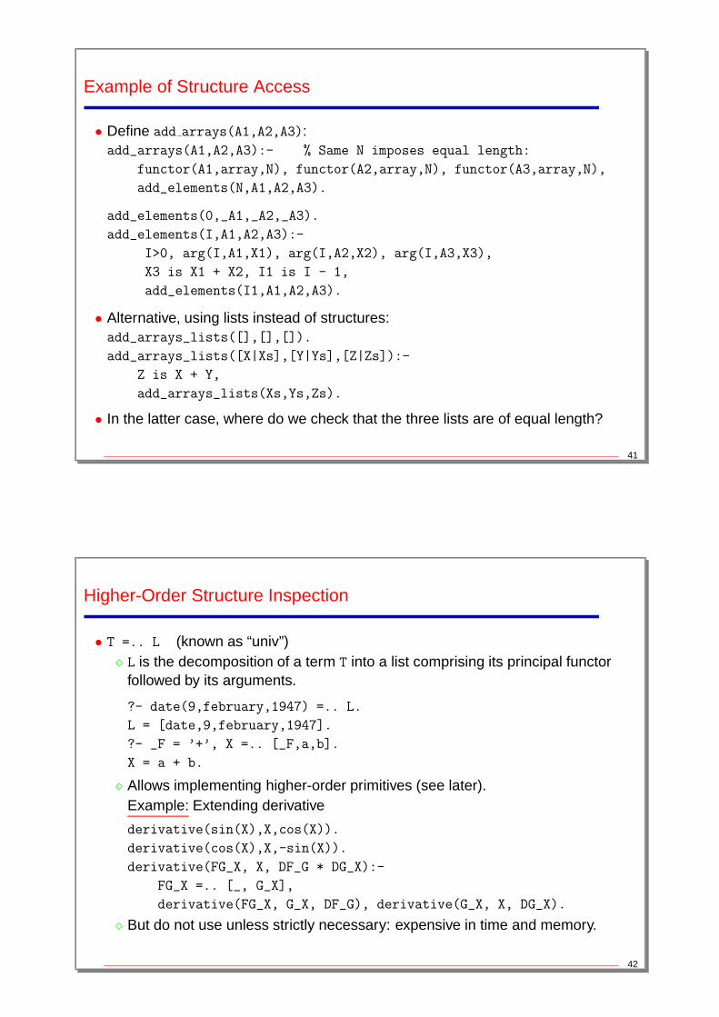
Structure Inspection (Contd.)

• arg(N, X, Arg):

� N integer, X compound term→ Arg unified with n-th argument of X.� Allows accessing a structure argument in constant time and in a compact way.� Error if N is not an integer, or if X is a free variable.� Fails if the unification fails.

Examples:

?- _T=date(9,February,1947), arg(3,_T,X).

X = 1947

?- _T=date(9,February,1947), _T=date(_,_,X).

X = 1947

?- functor(Array,array,5),

arg(1,Array,black),

arg(5,Array,white).

Array = array(black,_,_,_,white).

• What does ?- arg(2,[a,b,c,d],X). return?

39

Example of Structure Inspection

• Define subterm(Sub,Term) (Term will always be a compound term):

subterm(Term,Term).

subterm(Sub,Term):-

functor(Term,F,N),

subterm(N,Sub,Term).

subterm(N,Sub,Term):-

arg(N,Term,Arg), % also checks N > 0 (arg/1 fails otherwise!)

subterm(Sub,Arg).

subterm(N,Sub,Term):-

N>1,

N1 is N-1,

subterm(N1,Sub,Term).

40

Example of Structure Access

• Define add arrays(A1,A2,A3):add_arrays(A1,A2,A3):- % Same N imposes equal length:

functor(A1,array,N), functor(A2,array,N), functor(A3,array,N),

add_elements(N,A1,A2,A3).

add_elements(0,_A1,_A2,_A3).

add_elements(I,A1,A2,A3):-

I>0, arg(I,A1,X1), arg(I,A2,X2), arg(I,A3,X3),

X3 is X1 + X2, I1 is I - 1,

add_elements(I1,A1,A2,A3).

• Alternative, using lists instead of structures:add_arrays_lists([],[],[]).

add_arrays_lists([X|Xs],[Y|Ys],[Z|Zs]):-

Z is X + Y,

add_arrays_lists(Xs,Ys,Zs).

• In the latter case, where do we check that the three lists are of equal length?

41

Higher-Order Structure Inspection

• T =.. L (known as “univ”)� L is the decomposition of a term T into a list comprising its principal functor

followed by its arguments.

?- date(9,february,1947) =.. L.

L = [date,9,february,1947].

?- _F = ’+’, X =.. [_F,a,b].

X = a + b.

� Allows implementing higher-order primitives (see later).Example: Extending derivative

derivative(sin(X),X,cos(X)).

derivative(cos(X),X,-sin(X)).

derivative(FG_X, X, DF_G * DG_X):-

FG_X =.. [_, G_X],

derivative(FG_X, G_X, DF_G), derivative(G_X, X, DG_X).

� But do not use unless strictly necessary: expensive in time and memory.

42

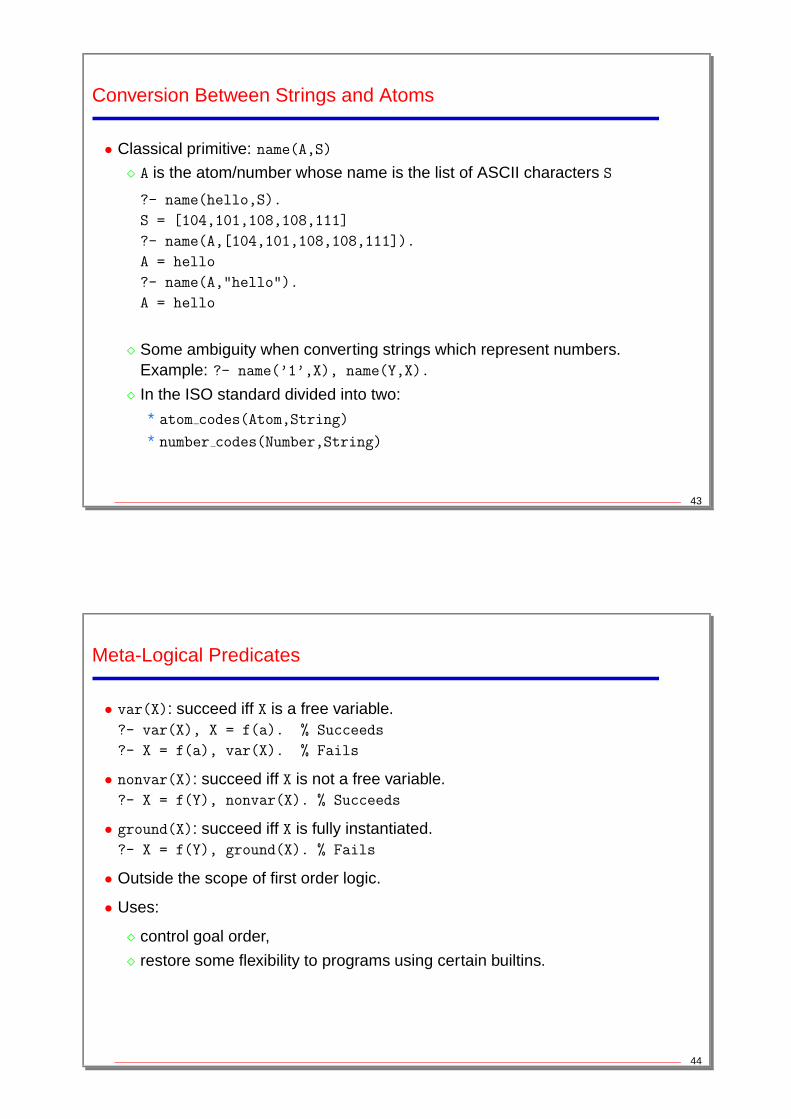
Conversion Between Strings and Atoms

• Classical primitive: name(A,S)

� A is the atom/number whose name is the list of ASCII characters S

?- name(hello,S).

S = [104,101,108,108,111]

?- name(A,[104,101,108,108,111]).

A = hello

?- name(A,"hello").

A = hello

� Some ambiguity when converting strings which represent numbers.Example: ?- name(’1’,X), name(Y,X).

� In the ISO standard divided into two:

* atom codes(Atom,String)

* number codes(Number,String)

43

Meta-Logical Predicates

• var(X): succeed iff X is a free variable.?- var(X), X = f(a). % Succeeds

?- X = f(a), var(X). % Fails

• nonvar(X): succeed iff X is not a free variable.?- X = f(Y), nonvar(X). % Succeeds

• ground(X): succeed iff X is fully instantiated.?- X = f(Y), ground(X). % Fails

• Outside the scope of first order logic.

• Uses:

� control goal order,

� restore some flexibility to programs using certain builtins.

44

Meta-Logical Predicates (Contd.)

• Example:

length(Xs,N):-

var(Xs), integer(N), length_num(N,Xs).

length(Xs,N):-

nonvar(Xs), length_list(Xs,N).

length_num(0,[]).

length_num(N,[_|Xs]):-

N > 0, N1 is N - 1, length_num(N1,Xs).

length_list([],0).

length_list([X|Xs],N):-

length_list(Xs,N1), N is N1 + 1.

• But note that it is not really needed: the normal definition of length is actuallyreversible!

45

Comparing Non-ground Terms

• Many applications need comparisons between non–ground/non–numeric terms.

• Identity tests:

� X == Y (identical)

� X \== Y (not identical)

?- f(X) == f(X). %Succeeds

?- f(X) == f(Y). %Fails

• Term ordering:

� X @> Y, X @>= Y, X @< Y, X @=< Y (alphabetic/lexicographic order)

?- f(a) @> f(b). %Fails

?- f(b) @> f(a). %Succeeds

?- f(X) @> f(Y). %Implementation dependent!

46

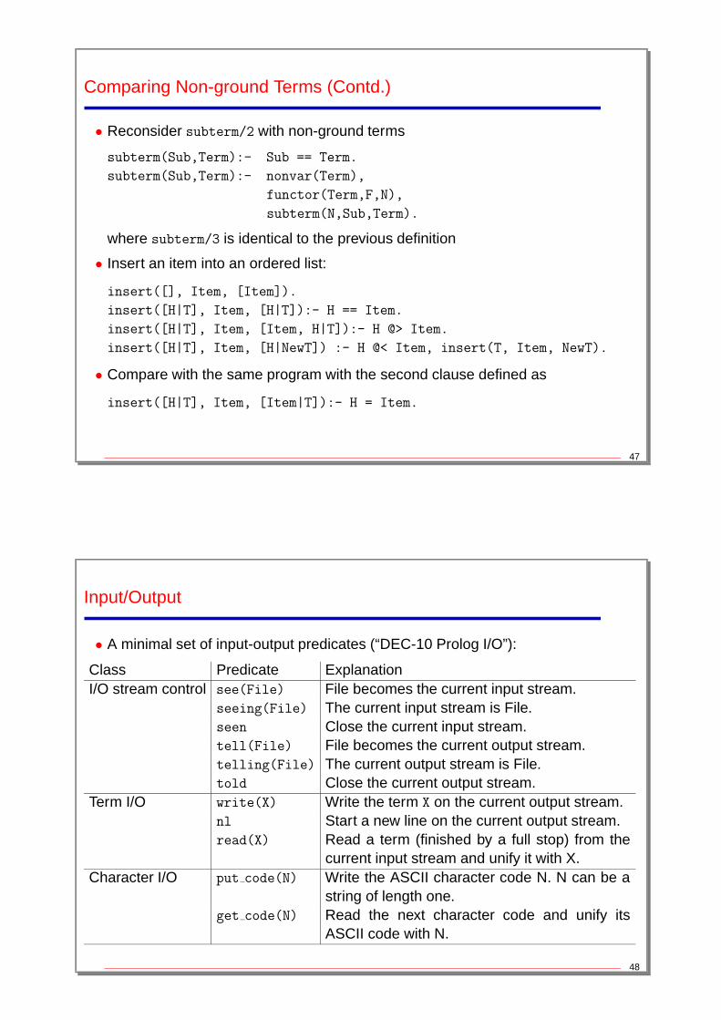
Comparing Non-ground Terms (Contd.)

• Reconsider subterm/2 with non-ground terms

subterm(Sub,Term):- Sub == Term.

subterm(Sub,Term):- nonvar(Term),

functor(Term,F,N),

subterm(N,Sub,Term).

where subterm/3 is identical to the previous definition

• Insert an item into an ordered list:

insert([], Item, [Item]).

insert([H|T], Item, [H|T]):- H == Item.

insert([H|T], Item, [Item, H|T]):- H @> Item.

insert([H|T], Item, [H|NewT]) :- H @< Item, insert(T, Item, NewT).

• Compare with the same program with the second clause defined as

insert([H|T], Item, [Item|T]):- H = Item.

47

Input/Output

• A minimal set of input-output predicates (“DEC-10 Prolog I/O”):

Class Predicate ExplanationI/O stream control see(File) File becomes the current input stream.

seeing(File) The current input stream is File.seen Close the current input stream.tell(File) File becomes the current output stream.telling(File) The current output stream is File.told Close the current output stream.

Term I/O write(X) Write the term X on the current output stream.nl Start a new line on the current output stream.read(X) Read a term (finished by a full stop) from the

current input stream and unify it with X.Character I/O put code(N) Write the ASCII character code N. N can be a

string of length one.get code(N) Read the next character code and unify its

ASCII code with N.

48

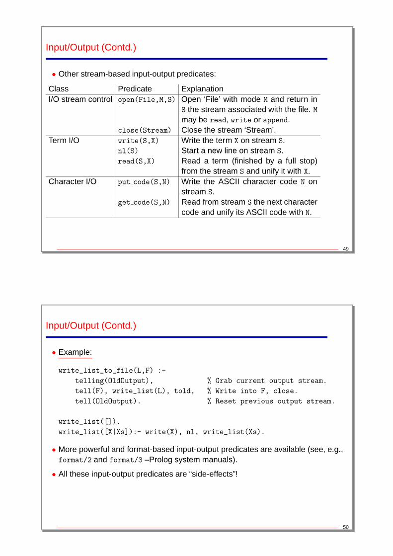
Input/Output (Contd.)

• Other stream-based input-output predicates:

Class Predicate ExplanationI/O stream control open(File,M,S) Open ‘File’ with mode M and return in

S the stream associated with the file. Mmay be read, write or append.

close(Stream) Close the stream ‘Stream’.Term I/O write(S,X) Write the term X on stream S.

nl(S) Start a new line on stream S.read(S,X) Read a term (finished by a full stop)

from the stream S and unify it with X.Character I/O put code(S,N) Write the ASCII character code N on

stream S.get code(S,N) Read from stream S the next character

code and unify its ASCII code with N.

49

Input/Output (Contd.)

• Example:

write_list_to_file(L,F) :-

telling(OldOutput), % Grab current output stream.

tell(F), write_list(L), told, % Write into F, close.

tell(OldOutput). % Reset previous output stream.

write_list([]).

write_list([X|Xs]):- write(X), nl, write_list(Xs).

• More powerful and format-based input-output predicates are available (see, e.g.,format/2 and format/3 –Prolog system manuals).

• All these input-output predicates are “side-effects”!

50

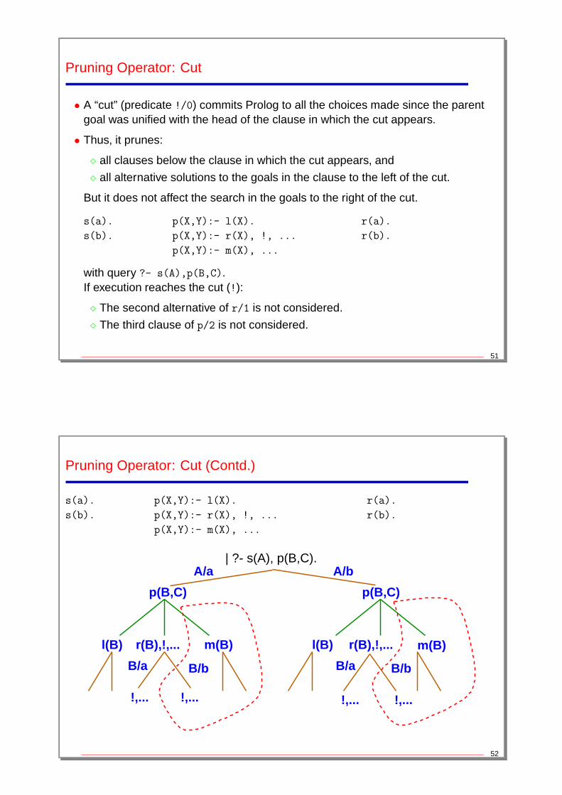
Pruning Operator: Cut

• A “cut” (predicate !/0) commits Prolog to all the choices made since the parentgoal was unified with the head of the clause in which the cut appears.

• Thus, it prunes:

� all clauses below the clause in which the cut appears, and

� all alternative solutions to the goals in the clause to the left of the cut.

But it does not affect the search in the goals to the right of the cut.

s(a). p(X,Y):- l(X). r(a).

s(b). p(X,Y):- r(X), !, ... r(b).

p(X,Y):- m(X), ...

with query ?- s(A),p(B,C).If execution reaches the cut (!):

� The second alternative of r/1 is not considered.

� The third clause of p/2 is not considered.

51

Pruning Operator: Cut (Contd.)

s(a). p(X,Y):- l(X). r(a).

s(b). p(X,Y):- r(X), !, ... r(b).

p(X,Y):- m(X), ...

p(B,C)

l(B)

B/a

!,...

l(B) m(B)

p(B,C)

A/bA/a

m(B)

B/b B/bB/a

r(B),!,...

| ?- s(A), p(B,C).

!,... !,...!,...

r(B),!,...

52

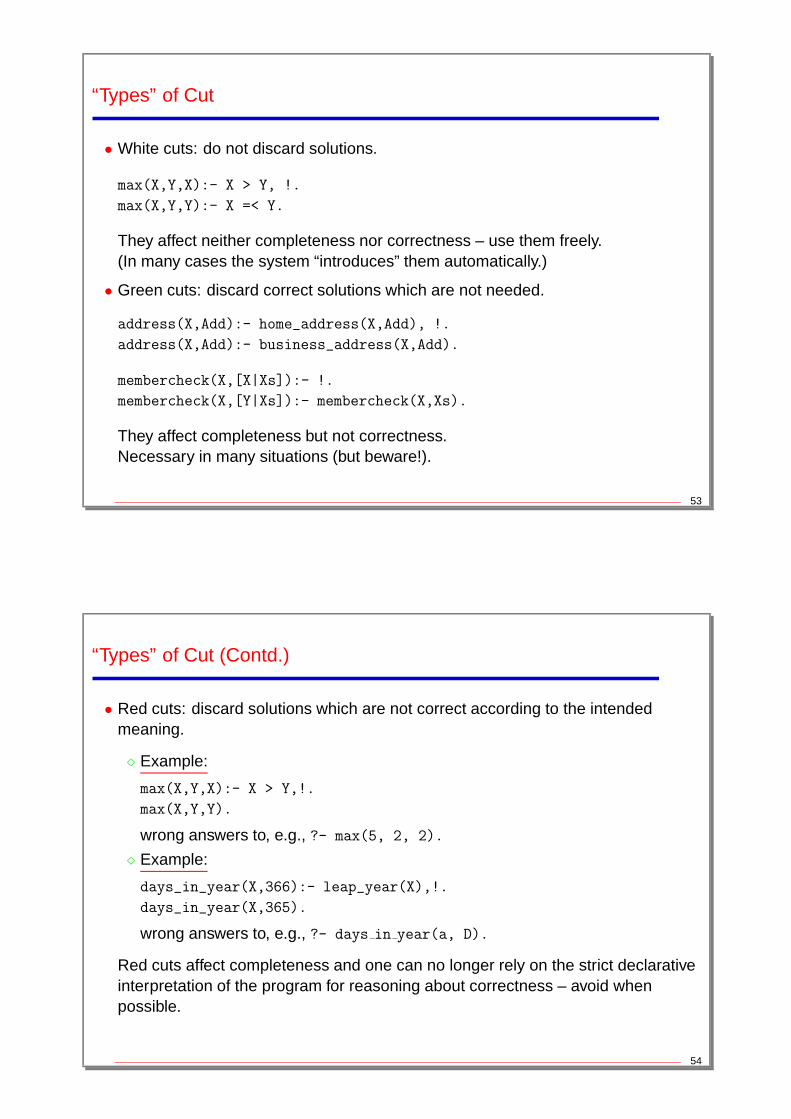
“Types” of Cut

• White cuts: do not discard solutions.

max(X,Y,X):- X > Y, !.

max(X,Y,Y):- X =< Y.

They affect neither completeness nor correctness – use them freely.(In many cases the system “introduces” them automatically.)

• Green cuts: discard correct solutions which are not needed.

address(X,Add):- home_address(X,Add), !.

address(X,Add):- business_address(X,Add).

membercheck(X,[X|Xs]):- !.

membercheck(X,[Y|Xs]):- membercheck(X,Xs).

They affect completeness but not correctness.Necessary in many situations (but beware!).

53

“Types” of Cut (Contd.)

• Red cuts: discard solutions which are not correct according to the intendedmeaning.

� Example:

max(X,Y,X):- X > Y,!.

max(X,Y,Y).

wrong answers to, e.g., ?- max(5, 2, 2).

� Example:

days_in_year(X,366):- leap_year(X),!.

days_in_year(X,365).

wrong answers to, e.g., ?- days in year(a, D).

Red cuts affect completeness and one can no longer rely on the strict declarativeinterpretation of the program for reasoning about correctness – avoid whenpossible.

54

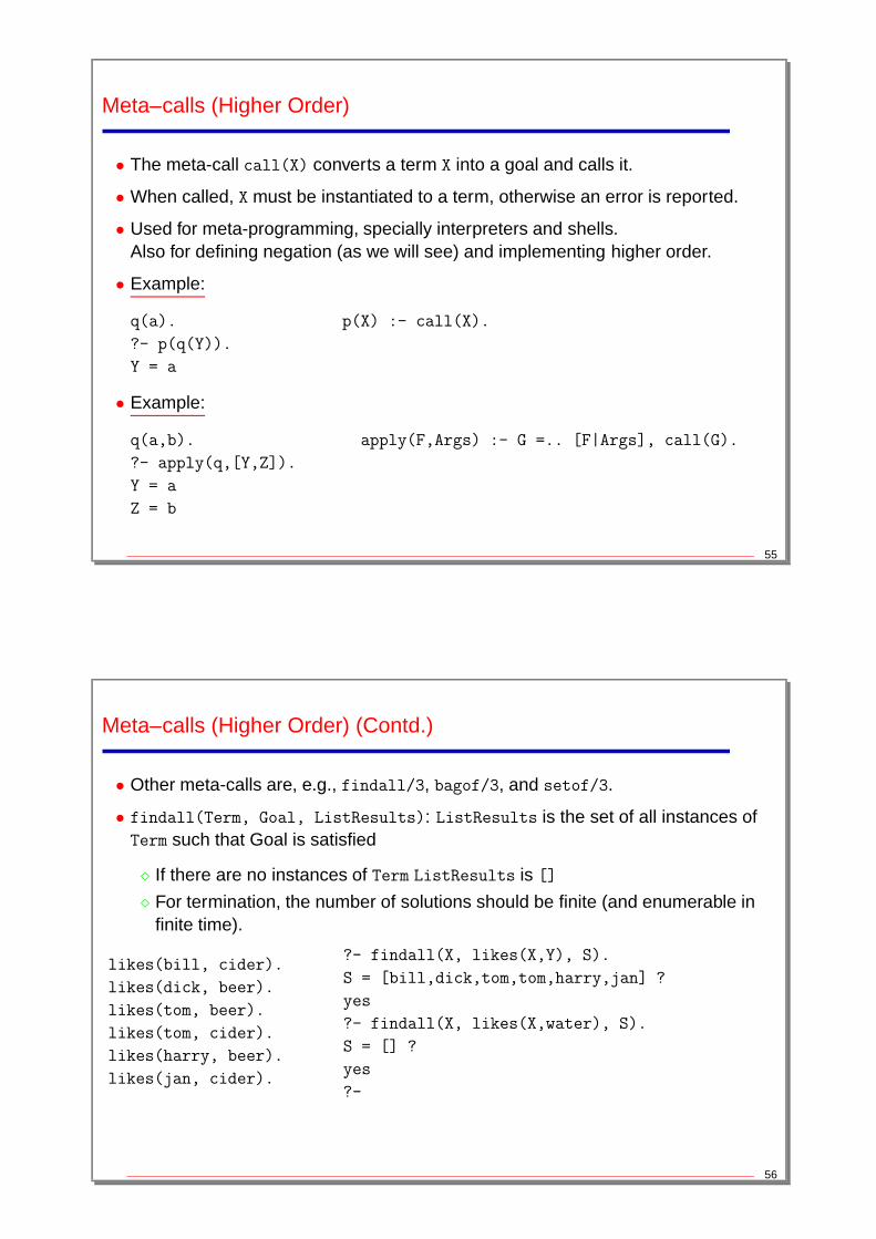
Meta–calls (Higher Order)

• The meta-call call(X) converts a term X into a goal and calls it.

• When called, X must be instantiated to a term, otherwise an error is reported.

• Used for meta-programming, specially interpreters and shells.Also for defining negation (as we will see) and implementing higher order.

• Example:

q(a). p(X) :- call(X).

?- p(q(Y)).

Y = a

• Example:

q(a,b). apply(F,Args) :- G =.. [F|Args], call(G).

?- apply(q,[Y,Z]).

Y = a

Z = b

55

Meta–calls (Higher Order) (Contd.)

• Other meta-calls are, e.g., findall/3, bagof/3, and setof/3.

• findall(Term, Goal, ListResults): ListResults is the set of all instances ofTerm such that Goal is satisfied

� If there are no instances of Term ListResults is []

� For termination, the number of solutions should be finite (and enumerable infinite time).

likes(bill, cider).

likes(dick, beer).

likes(tom, beer).

likes(tom, cider).

likes(harry, beer).

likes(jan, cider).

?- findall(X, likes(X,Y), S).

S = [bill,dick,tom,tom,harry,jan] ?

yes

?- findall(X, likes(X,water), S).

S = [] ?

yes

?-

56

Meta–calls (Higher Order) (Contd.)

• setof(Term, Goal, ListResults): ListResults is the ordered set (noduplicates) of all instances of Term such that Goal is satisfied

� If there are no instances of Term the predicate fails

� The set should be finite (and enumerable in finite time)

� If there are un-instantiated variables in Goal which do not also appear in Term

then a call to this built-in predicate may backtrack, generating alternativevalues for ListResults corresponding to different instantiations of the freevariables of Goal

� Variables in Goal will not be treated as free if they are explicitly bound withinGoal by an existential quantifier as in Y^...

(then, they behave as in findall/3)

• bagof/3 same, but returns list unsorted and with duplicates (in backtrackingorder)

57

Meta-calls: Examples

likes(bill, cider).

likes(dick, beer).

likes(harry, beer).

likes(jan, cider).

likes(tom, beer).

likes(tom, cider).

?- setof(X, likes(X,Y), S).

S = [dick,harry,tom],

Y = beer ? ;

S = [bill,jan,tom],

Y = cider ? ;

no

?- setof((Y,S), setof(X, likes(X,Y), S), SS).

SS = [(beer,[dick,harry,tom]),

(cider,[bill,jan,tom])] ? ;

no

?- setof(X, Y^(likes(X,Y)), S).

S = [bill,dick,harry,jan,tom] ? ;

no

58

Negation as Failure

• Uses the meta-call facilities, the cut and a system predicate fail that fails whenexecuted (similar to calling a=b).

not(Goal) :- call(Goal), !, fail.

not(Goal).

• Available as the (prefix) predicate \+/1: \+ member(c, [a,k,l])

• It will never instantiate variables.

• Termination of not(Goal) depends on termination of Goal. not(Goal) willterminate if a success node for Goal is found before an infinite branch.

• It is very useful but dangerous:

unmarried_student(X):- not(married(X)), student(X).

student(joe).

married(john).

• Works properly for ground goals (programmer’s responsibility to ensure this).

59

Cut-Fail

• Cut-fail combinations allow forcing the failure of a predicate — somehowspecifying a negative answer (useful but very dangerous!).

• Example – testing groundness: fail as soon as a free variable is found.

ground(Term):- var(Term), !, fail.

ground(Term):-

nonvar(Term),

functor(Term,F,N),

ground(N,Term).

ground(0,T). %% All subterms traversed

ground(N,T):-

N>0,

arg(N,T,Arg),

ground(Arg),

N1 is N-1,

ground(N1,T).

60

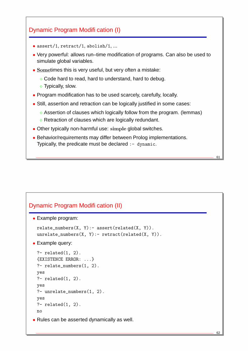
Dynamic Program Modification (I)

• assert/1, retract/1, abolish/1, ...

• Very powerful: allows run–time modification of programs. Can also be used tosimulate global variables.

• Sometimes this is very useful, but very often a mistake:

� Code hard to read, hard to understand, hard to debug.

� Typically, slow.

• Program modification has to be used scarcely, carefully, locally.

• Still, assertion and retraction can be logically justified in some cases:

� Assertion of clauses which logically follow from the program. (lemmas)

� Retraction of clauses which are logically redundant.

• Other typically non-harmful use: simple global switches.

• Behavior/requirements may differ between Prolog implementations.Typically, the predicate must be declared :- dynamic.

61

Dynamic Program Modification (II)

• Example program:

relate_numbers(X, Y):- assert(related(X, Y)).

unrelate_numbers(X, Y):- retract(related(X, Y)).

• Example query:

?- related(1, 2).

{EXISTENCE ERROR: ...}

?- relate_numbers(1, 2).

yes

?- related(1, 2).

yes

?- unrelate_numbers(1, 2).

yes

?- related(1, 2).

no

• Rules can be asserted dynamically as well.

62

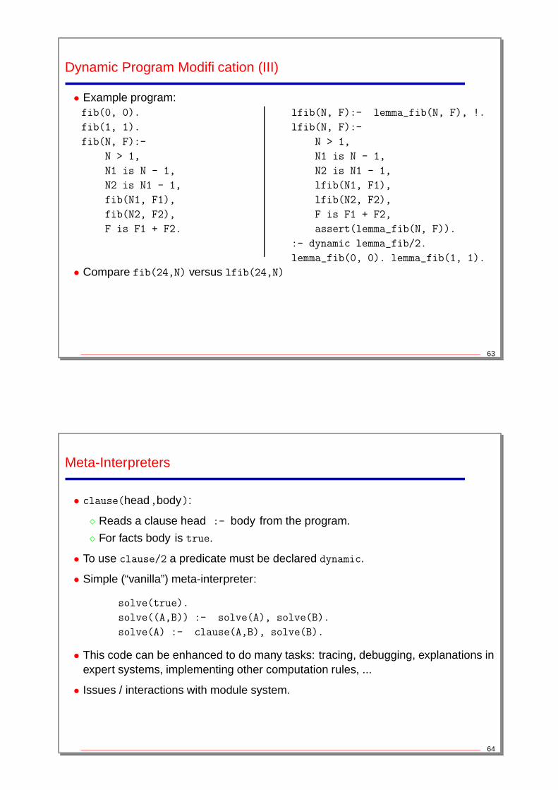
Dynamic Program Modification (III)

• Example program:fib(0, 0).

fib(1, 1).

fib(N, F):-

N > 1,

N1 is N - 1,

N2 is N1 - 1,

fib(N1, F1),

fib(N2, F2),

F is F1 + F2.

lfib(N, F):- lemma_fib(N, F), !.

lfib(N, F):-

N > 1,

N1 is N - 1,

N2 is N1 - 1,

lfib(N1, F1),

lfib(N2, F2),

F is F1 + F2,

assert(lemma_fib(N, F)).

:- dynamic lemma_fib/2.

lemma_fib(0, 0). lemma_fib(1, 1).

• Compare fib(24,N) versus lfib(24,N)

63

Meta-Interpreters

• clause(head,body):

� Reads a clause head :- body from the program.

� For facts body is true.

• To use clause/2 a predicate must be declared dynamic.

• Simple (“vanilla”) meta-interpreter:

solve(true).

solve((A,B)) :- solve(A), solve(B).

solve(A) :- clause(A,B), solve(B).

• This code can be enhanced to do many tasks: tracing, debugging, explanations inexpert systems, implementing other computation rules, ...

• Issues / interactions with module system.

64

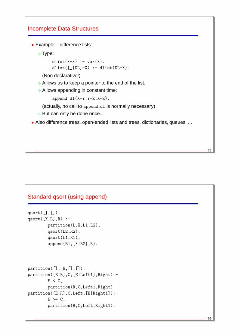
Incomplete Data Structures

• Example – difference lists:

� Type:

dlist(X-X) :- var(X).

dlist([_|DL]-X) :- dlist(DL-X).

(Non declarative!)

� Allows us to keep a pointer to the end of the list.

� Allows appending in constant time:

append_dl(X-Y,Y-Z,X-Z).

(actually, no call to append dl is normally necessary)

� But can only be done once...

• Also difference trees, open-ended lists and trees, dictionaries, queues, ...

65

Standard qsort (using append)

qsort([],[]).

qsort([X|L],R) :-

partition(L,X,L1,L2),

qsort(L2,R2),

qsort(L1,R1),

append(R1,[X|R2],R).

partition([],_B,[],[]).

partition([E|R],C,[E|Left1],Right):-

E < C,

partition(R,C,Left1,Right).

partition([E|R],C,Left,[E|Right1]):-

E >= C,

partition(R,C,Left,Right1).

66

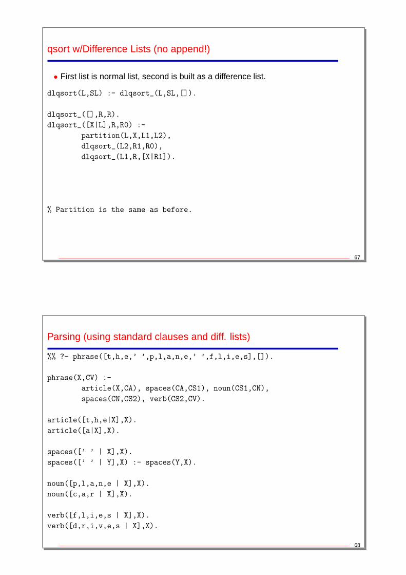
qsort w/Difference Lists (no append!)

• First list is normal list, second is built as a difference list.

dlqsort(L,SL) :- dlqsort_(L,SL,[]).

dlqsort_([],R,R).

dlqsort_([X|L],R,R0) :-

partition(L,X,L1,L2),

dlqsort_(L2,R1,R0),

dlqsort_(L1,R,[X|R1]).

% Partition is the same as before.

67

Parsing (using standard clauses and diff. lists)

%% ?- phrase([t,h,e,’ ’,p,l,a,n,e,’ ’,f,l,i,e,s],[]).

phrase(X,CV) :-

article(X,CA), spaces(CA,CS1), noun(CS1,CN),

spaces(CN,CS2), verb(CS2,CV).

article([t,h,e|X],X).

article([a|X],X).

spaces([’ ’ | X],X).

spaces([’ ’ | Y],X) :- spaces(Y,X).

noun([p,l,a,n,e | X],X).

noun([c,a,r | X],X).

verb([f,l,i,e,s | X],X).

verb([d,r,i,v,e,s | X],X).

68

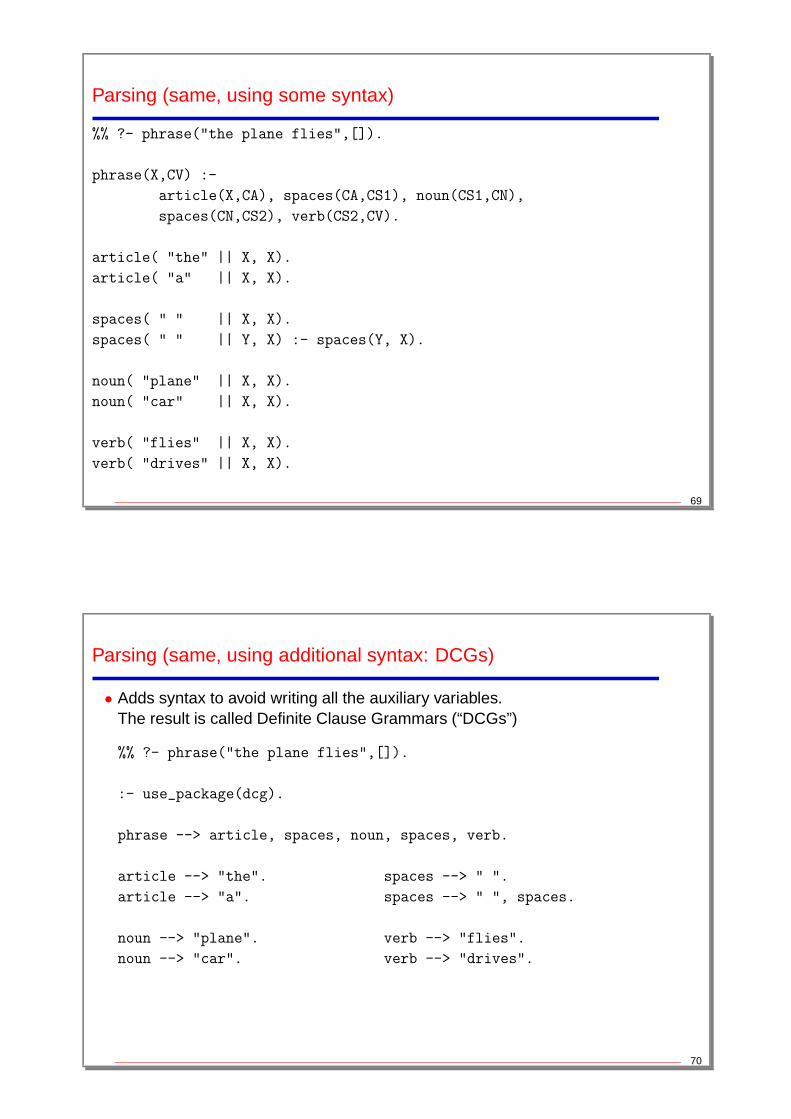
Parsing (same, using some syntax)

%% ?- phrase("the plane flies",[]).

phrase(X,CV) :-

article(X,CA), spaces(CA,CS1), noun(CS1,CN),

spaces(CN,CS2), verb(CS2,CV).

article( "the" || X, X).

article( "a" || X, X).

spaces( " " || X, X).

spaces( " " || Y, X) :- spaces(Y, X).

noun( "plane" || X, X).

noun( "car" || X, X).

verb( "flies" || X, X).

verb( "drives" || X, X).

69

Parsing (same, using additional syntax: DCGs)

• Adds syntax to avoid writing all the auxiliary variables.The result is called Definite Clause Grammars (“DCGs”)

%% ?- phrase("the plane flies",[]).

:- use_package(dcg).

phrase --> article, spaces, noun, spaces, verb.

article --> "the". spaces --> " ".

article --> "a". spaces --> " ", spaces.

noun --> "plane". verb --> "flies".

noun --> "car". verb --> "drives".

70

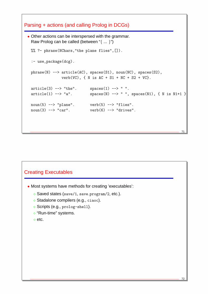
Parsing + actions (and calling Prolog in DCGs)

• Other actions can be interspersed with the grammar.Raw Prolog can be called (between “{ ... }”)

%% ?- phrase(NChars,"the plane flies",[]).

:- use_package(dcg).

phrase(N) --> article(AC), spaces(S1), noun(NC), spaces(S2),

verb(VC), { N is AC + S1 + NC + S2 + VC}.

article(3) --> "the". spaces(1) --> " ".

article(1) --> "a". spaces(N) --> " ", spaces(N1), { N is N1+1 }.

noun(5) --> "plane". verb(5) --> "flies".

noun(3) --> "car". verb(6) --> "drives".

71

Creating Executables

• Most systems have methods for creating ’executables’:

� Saved states (save/1, save program/2, etc.).

� Stadalone compilers (e.g., ciaoc).

� Scripts (e.g., prolog-shell).

� “Run-time” systems.

� etc.

72

Other issues in Prolog (see “The Art of Prolog” and Bibliography)

• Extending the syntax (operators and term expansions/macros)

• Repeat loops.

• Modules (and objects).

• Delay declarations/concurrency.

• Graphical and source debuggers.

• Foreign language (e.g., C) interfaces.

• Native code compilation/creating executables.

• Exception handling

• Operating system interface (and sockets)

• ...

73

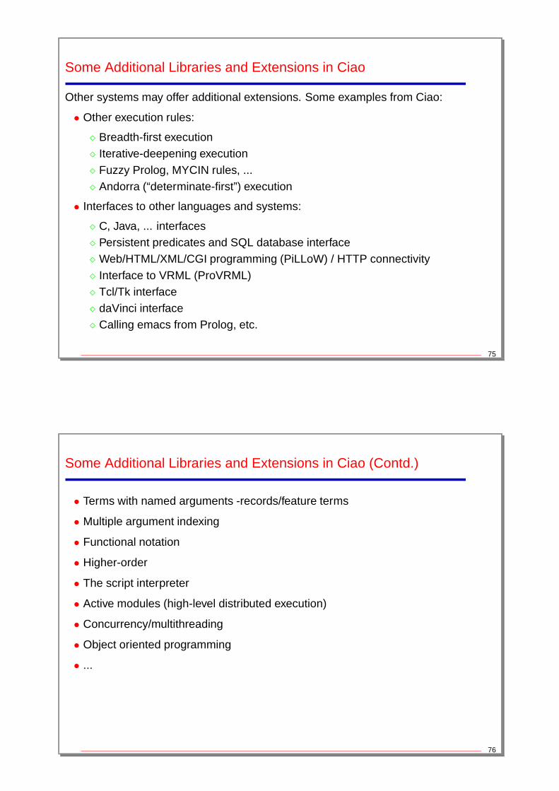
Some Typical Libraries in Prolog Systems

• Most systems have a good set of libraries.

• Worth checking before re-implementing existing functionality!

• Some examples:

Arrays Assoc Attributes HeapsLists Term Utilities Ordset Queues

Random System Utilities Tree UGraphsWGraphs Sockets Linda/Distribution Persistent DB

CLPB CLPQR CLPFD ObjectsGCLA TclTk Tracing Chars I/O

Runtime Utilities Timeout Xrefs WWWJava Interface ... ... ...

74

Some Additional Libraries and Extensions in Ciao

Other systems may offer additional extensions. Some examples from Ciao:

• Other execution rules:

� Breadth-first execution� Iterative-deepening execution� Fuzzy Prolog, MYCIN rules, ...� Andorra (“determinate-first”) execution

• Interfaces to other languages and systems:

� C, Java, ... interfaces� Persistent predicates and SQL database interface� Web/HTML/XML/CGI programming (PiLLoW) / HTTP connectivity� Interface to VRML (ProVRML)� Tcl/Tk interface� daVinci interface� Calling emacs from Prolog, etc.

75

Some Additional Libraries and Extensions in Ciao (Contd.)

• Terms with named arguments -records/feature terms

• Multiple argument indexing

• Functional notation

• Higher-order

• The script interpreter

• Active modules (high-level distributed execution)

• Concurrency/multithreading

• Object oriented programming

• ...

76

Other Issues / To Learn More

• Assertions:

� Regular types

� Modes

� Properties which are native to analyzers

� Run-time checking of assertions

• Constraint programming (CLP)

� rationals, reals, finite domains, ...

• Advanced programming environments:

� Compile-time type, mode, and property inference and checking, ...(preprocessors).

� Automatic documentation.

� ...

77