computational issues related to cfa mplus model command for

65

129

Computational Issues Related To CFA• Scale of observed variables – important to keep them on a similar

scale

• Convergence – often related to starting values or the type of model being estimated

• Program stops because maximum number of iterations has been reached

• If no negative residual variances, either increase the number of iterations or use the preliminary parameter estimates as starting values

• If there are large negative residual variances, try better starting values

• Program stops before the maximum number of iterations has been reached

• Check if variables are on a similar scale• Try new starting values

• Starting values – the most important parameters to give starting values to are residual variances

130

Mplus MODEL Command For CFAMODEL command is used to describe the model to be estimated

BY statement is used to define the latent variables or factors

BY is short for “measured by”

Example 1 – standard parameterization

MODEL: f1 BY y1 y2 y3;f2 BY y4 y5 y6;

Defaults• Factor loading of first variable after BY is fixed to one• Factor loadings of other variables are estimated• Residual variances are estimated• Residual covariances are fixed to zero• Variances of factors are estimated• Covariance between the exogenous factors is estimated

66

131

Example 2 – Alternative parameterization

MODEL: f1 BY y1* y2 y3;f2 BY y4* y5 y6;f1@1 f2@1; ! or f1-f2@1;

Mplus MODEL Command For CFA(Continued)

132

EFA In A CFA Framework

*

67

133

EFA In A CFA FrameworkJöreskog, K.G. (1969)• Purpose

• To obtain standard errors to determine if factor loadings are statistically significant

• To obtain modification indices to determine if residual covariances are needed to represent minor factors

• Use the same number of restrictions as an exploratory factor analysis model – m2

• Fix factor variances to one for m restrictions• Fix factor loadings to zero for the remaining restrictions

• Find an anchor item for each factor – select an item that has a large loading for the factor and small loadings for other factors

• Fix the loading of the anchor item to zero for all of the other factors

• Allow all other factor loadings to be free

• Will get the same model fit as EFA *

134

Promax Rotated Loadings – 3 Factor Solution

0.0760.3510.081FIGUREW

0.0350.0610.577VISUAL

0.043-0.1140.0100.8160.5720.8910.7770.728

-0.0100.033

-0.039

0.6780.5730.6110.0370.065

-0.0150.080

-0.029-0.0320.115

-0.114

0.127OBJECT0.116NUMBERR

-0.023WORDR0.015WORDM0.149WORDC

-0.060SENTENCE0.009PARAGRAP0.152GENERAL0.765LOZENGES0.434PAPER0.602CUBES

VerbalMemorySpatial

Selecting Anchor Items

*

68

135

ESTIMATOR = ML;ANALYSIS:

FILE IS holzall.dat;FORMAT IS f3,2f2,f3,2f2/3x,13(1x,f3)/3x,11(1x,f3);

DATA:

NAMES ARE id female grade agey agem school visual cubes paper lozenges general paragrap sentence wordcwordm addition code counting straight wordr numberrfigurer object numberf figurew deduct numeric problemr series arithmet;

USEV ARE visual cubes paper lozenges general paragrap sentence wordc wordm wordr numberr object figurew;

USEOBS IS school EQ 0;

VARIABLE:

EFA in a CFA framework using 13 variables from Holzinger and Swineford (1939)

TITLE:

Input For Holzinger-Swineford EFA In A CFA Framework Using 13 Variables

*

136

Input For Holzinger-Swineford EFA In A CFA Framework Using 13 Variables (Continued)

spatial BY visual-figurew*0 ! start all items at 0lozenges*1 ! start anchor item at 1cubes*1 ! start other large items at 1sentence@0 wordr@0; ! remove 2 indeterminacies

verbal BY visual-figurew*0 ! start all items at 0sentence*1 ! start anchor item at 1wordm*1 ! start other large items at 1lozenges@0 wordr@0; ! remove 2 indeterminacies

spatial-verbal@1; ! remove 3 indeterminacies

STANDARDIZED MODINDICES(3.84) SAMPSTAT FSDETERMINACY;OUTPUT:

memory BY visual-figurew*0 ! start all items at 0wordr*1 ! start anchor item at 1object*1 ! start other large items at 1lozenges@0 sentence@0; ! remove 2 indeterminacies

MODEL:

*

69

137

Tests Of Model Fit

0.949Probability RMSEA <= .05SRMR (Standardized Root Mean Square Residual)

0.028Value

0.00090 Percent C.I.0.000Estimate

39.028Value42Degrees of Freedom

0.6022P-Value

1.009TLI

Chi-Square Test of Model Fit

CFI

RMSEA (Root Mean Square Error Of Approximation)

CFI/TLI1.000

Output Excerpts Holzinger-Swineford EFA In A CFA Framework Using 13 Variables

0.050

Factor Determinacies0.869SPATIAL0.841MEMORY0.948VERBAL *

138

Model Results

0.793-0.6610.9380.0000.7801.8890.0000.6922.1498.0713.7174.6204.848

0.4410.6631.0190.0000.7100.5260.0000.3071.0600.7650.3270.5590.811

0.0980.3500.350FIGUREW-0.096-0.439-0.439OBJECT0.1270.9560.956NUMBERR0.0000.0000.000WORDR0.0700.5540.554WORDM0.1860.9940.994WORDC0.0000.0000.000SENTENCE0.0630.2120.212PARAGRAP0.1962.2782.278GENERAL0.7456.1736.173LOZENGES0.4321.2161.216PAPER0.5832.5842.584CUBES0.5713.9333.933VISUAL

SPATIAL BY

Est./S.E.S.E. StdYXStdEstimates

Output Excerpts Holzinger-Swineford EFA In A CFA Framework Using 13 Variables (Continued)

*

*Note that theory predicts that GENERAL loads on VERBAL only.

*

70

139

2.9234.7044.3926.1800.5900.8080.0001.030

-0.0910.0001.123

-0.7120.718

0.4330.6460.9771.0580.7200.5400.0000.3091.1030.0000.3330.5580.808

0.3531.2641.264FIGUREW0.6683.0403.040OBJECT0.5714.2914.291NUMBERR0.6066.5416.541WORDR0.0540.4250.425WORDM0.0820.4360.436WORDC0.0000.0000.000SENTENCE0.0940.3180.318PARAGRAP

-0.009-0.100-0.100GENERAL0.0000.0000.000LOZENGES0.1330.3740.374PAPER

-0.090-0.398-0.398CUBES0.0840.5800.580VISUAL

MEMORY BY



*

140

0.5700.212

-0.8420.0008.7515.656

12.2638.2647.6820.0000.294

-0.2360.326

0.4330.6531.0330.0000.7070.5170.3220.3031.0580.0000.3270.5460.811

0.0690.2470.247FIGUREW0.0300.1390.139OBJECT

-0.116-0.870-0.870NUMBERR0.0000.0000.000WORDR0.7826.1916.191WORDM0.5482.9272.927WORDC0.8533.9543.954SENTENCE0.7442.5012.501PARAGRAP0.7008.1308.130GENERAL0.0000.000.000LOZENGES0.0340.0960.096PAPER

-0.029-0.129-0.129CUBES0.0380.2650.265VISUAL

VERBAL BY



*

71

141


Variances1.0001.0000.0000.0001.000SPATIAL1.0001.0000.0000.0001.000VERBAL1.0001.0000.0000.0001.000MEMORY

3.1812.173

3.937

0.1440.171

0.119

0.4590.4590.459VERBAL0.3710.3710.371SPATIAL

MEMORY WITH

0.4670.4670.467SPATIALVERBAL WITH


*

142


7.8605.0226.2685.9246.2987.8035.5986.6846.9234.3387.6196.7326.649

1.3192.3775.998

12.4222.8781.8641.0420.5446.8247.0630.7612.0494.325

0.80710.36810.368FIGUREW0.57611.93911.939OBJECT0.66537.59537.595NUMBERR0.63273.58973.589WORDR0.28918.12218.122WORDM0.51014.54714.547WORDC0.2725.8315.831SENTENCE0.3213.6373.637PARAGRAP0.35047.23947.239GENERAL0.44630.64030.640LOZENGES0.7345.8015.801PAPER0.70313.79513.795CUBES0.60628.75828.758VISUAL

Residual VariancesEst./S.E.S.E. StdYXStdEstimates

*

72

143

R-Square

0.193FIGUREW0.424OBJECT0.335NUMBERR0.368WORDR0.711WORDM0.490WORDC0.728SENTENCE0.679PARAGRAP0.650GENERAL0.554LOZENGES0.266PAPER0.297CUBES0.394VISUAL

R-SquareObservedVariable


! 1 – STDYX (residual) = Reliability! when no covariates are in the model

! R-Square =

*

144

Model Modification Indices


-4.2389.5552.657

6.5577.1216.586

-0.116-4.238WORDM WITH SENTENCE0.1049.555WORDM WITH GENERAL0.1072.657WORDC WITH SENTENCE

WITH Statements

Std E.P.C.E.P.C. StdYX E.P.C.M.I.

*

73

145

Simple Structure CFA

146

spatial

lozenges

general

paragrap

sentence

wordc

wordm

wordr

number

object

figurew

visual

cubes

paper

verbal

memory

74

147

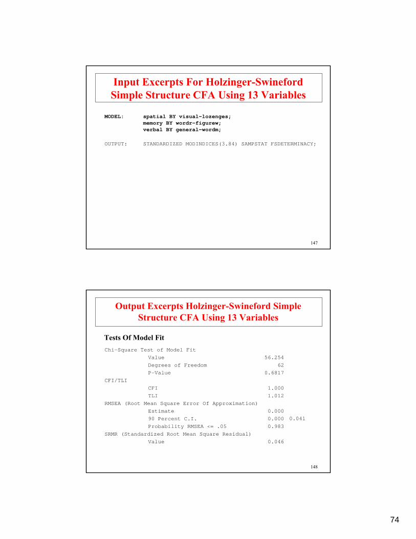
Input Excerpts For Holzinger-SwinefordSimple Structure CFA Using 13 Variables

spatial BY visual-lozenges;memory BY wordr-figurew;verbal BY general-wordm;

MODEL:

STANDARDIZED MODINDICES(3.84) SAMPSTAT FSDETERMINACY;OUTPUT:

148

Tests Of Model Fit


0.046Value



0.6817P-Value

1.012TLI


CFI


CFI/TLI1.000

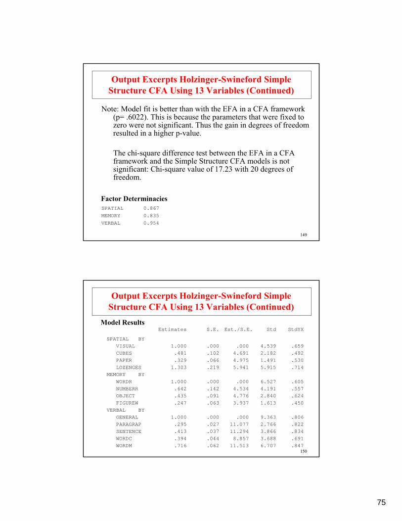
Output Excerpts Holzinger-Swineford SimpleStructure CFA Using 13 Variables

0.041

75

149

Factor Determinacies0.867SPATIAL0.835MEMORY0.954VERBAL

Note: Model fit is better than with the EFA in a CFA framework (p= .6022). This is because the parameters that were fixed to zero were not significant. Thus the gain in degrees of freedom resulted in a higher p-value.

The chi-square difference test between the EFA in a CFA framework and the Simple Structure CFA models is not significant: Chi-square value of 17.23 with 20 degrees of freedom.

Output Excerpts Holzinger-Swineford SimpleStructure CFA Using 13 Variables (Continued)

150

Model Results

MEMORY BY

11.5138.857

11.29411.077

.000

3.9374.7764.534.000

5.9414.9754.691.000

.062

.044

.037

.027

.000

.063

.091

.142

.000

.219

.066

.102

.000

.6913.688.394WORDC

.8343.866.413SENTENCE

.8222.766.295PARAGRAP

.8069.3631.000GENERALVERBAL BY

.4501.613.247FIGUREW

.6242.840.435OBJECT

.5574.191.642NUMBERR

.6056.5271.000WORDR

.7145.9151.303LOZENGES

.8476.707.716WORDM

.5301.491.329PAPER

.4922.182.481CUBES

.6594.5391.000VISUALSPATIAL BY


Output Excerpts Holzinger-Swineford Simple Structure CFA Using 13 Variables (Continued)

76

151

.522.5223.8238.34031.883VERBAL

3.2265.7053.779

3.077

4.407

13.20515.3635.450

4.329

5.700

1.0001.00042.606MEMORY1.0001.00087.646VERBAL1.0001.00020.597SPATIAL

Variances

.450.45013.323SPATIALMEMORY WITH

.591.59125.118SPATIALVERBAL WITH



152

R-Square

0.203FIGUREW0.389OBJECT0.311NUMBERR0.366WORDR0.717WORDM0.477WORDC0.696SENTENCE0.676PARAGRAP0.650GENERAL0.509LOZENGES0.281PAPER0.243CUBES0.434VISUAL


77

153

Model Modification Indices


7.5822.207

-3.108

7.5822.207

-3.108

0.0824.552WORDM WITH GENERAL0.0894.586WORDC WITH SENTENCE

-0.0804.170PARAGRAP WITH GENERAL

WITH StatementsStd E.P.C.E.P.C. StdYX E.P.C.M.I.

154

Special Factor Analysis Models

78

155

Bi-Factor Model

156

lozenges

general

paragrap

sentence

wordc

wordm

addition

code

counting

straight

visual

cubes

paper

object

numberf

figurew

deduct

numeric

problemr

series

arithmet

wordr

numberr

figurer

g

spatial

verbal

speed

recogn

memory

79

157

Input Excerpts Holzinger-Swineford General-Specific (Bi-Factor) Factor Model

uncorrelated factors because of the general factor:

g WITH spatial-memory @0;spatial WITH verbal-memory @0;verbal WITH speed-memory @0;speed WITH recogn-memory @0;recogn WITH memory @0;

!

STANDARDIZED MODINDICES(3.84) SAMPSTAT FSDTERMINACY;OUTPUT:

correlated residual (“doublet factor”):

addition WITH arithmet;

!

g BY visual-arithmet;spatial BY visual-lozenges;verbal BY general-wordm;speed BY addition-straight;recogn BY wordr-object;memory BY numberf object figurew;

MODEL:

158

Second-Order Factor Model

80

159

verbal

wk

gs

pc

as

ei

mc

cs

no

mk

ar

tech

speed

quant

g

160

Input For Second-OrderFactor Analysis Model

ESTIMATOR = ML;ANALYSIS:

FILE IS asvab.dat;! Armed services vocational aptitude batteryNOBSERVATIONS = 20422;TYPE=COVARIANCE;

DATA:

NAMES ARE ar wk pc mk gs no cs as mc ei;USEV = wk gs pc as ei mc cs no mk ar;

!WK Word Knowledge!GS General Science!PC Paragraph Comprehension!AS Auto and Shop Information!EI Electronics information!MC Mechanical Comprehension!CS Coding Speed!NO Numerical Operations!MK Mathematical Knowledge!AR Arithmetic Reasoning

VARIABLE:

Second-order factor analysis modelTITLE:

81

161

SAMPSTAT MOD(0) STAND TECH1 RESIDUAL;OUTPUT:

verbal BY wk gs pc ei;

tech BY gs mc ar;

speed BY pc cs no;

quant BY mk ar;

g BY verbal tech speed quant;

tech WITH verbal;

MODEL:

Input For Second-OrderFactor Analysis Model (Continued)

162

Bollen, K.A. (1989). Structural equations with latent variables. New York: John Wiley.

Joreskog, K.G. (1969). A general approach to confirmatory maximum likelihood factor analysis. Psychometrika, 34, 183-202.

Lawley, D.N. & Maxwell, A.E. (1971). Factor analysis as a statistical method. London: Butterworths.

Long, S. (1983). Confirmatory factor analysis. Sage University Paper series on Quantitative Applications in the Social Sciences, No 33. Beverly Hills, CA: Sage.

Mulaik, S. (1972). The foundations of factor analysis. McGraw-Hill.

Further Readings On CFA

82

163

Measurement Invariance AndPopulation Heterogeneity

164

To further study a set of factors or latent variables establishedby an EFA/CFA, questions can be asked about the invarianceof the measures and the heterogeneity of populations.

Measurement Invariance – Does the factor model hold inother populations or at other time points?

• Same number of factors• Zero loadings in the same positions• Equality of factor loadings• Equality of intercepts

• Test difficulty

Models To Study Measurement InvarianceAnd Population Heterogeneity

Population Heterogeneity – Are the factor means, variances, and covariances the same for different populations?

83

165

Models To Study Measurement Invariance and Population Heterogeneity

• CFA with covariates• Parsimonious• Small sample advantage• Advantageous with many groups

• Multiple group analysis• More parameters to represent non-invariance

• Factor loadings and observed residual variances/covariances in addition to intercepts

• Factor variances and covariances in addition to means• Interactions

Models To Study Measurement InvarianceAnd Population Heterogeneity (Continued)

166

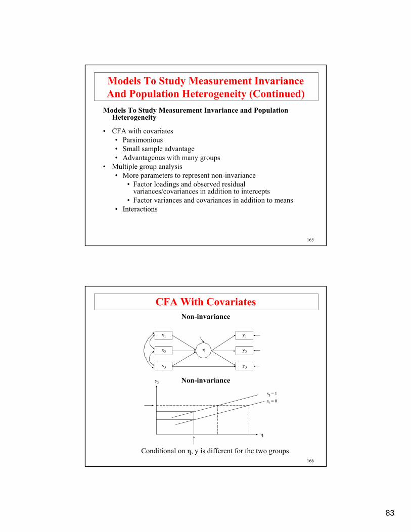
CFA With CovariatesNon-invariance

η

y1

y2

y3

x1

x2

x3

y3

x3 = 1

x3 = 0

η

Non-invariance

Conditional on η, y is different for the two groups

84

167

Multiple Group AnalysisInvariancey

Group A = Group B

η

y Group B

Group A

η

Non-invariance

168

CFA With Covariates (MIMIC)

85

169

Used to study the effects of covariates or background variables on the factors and outcome variables to understand measurement invariance and heterogeneity

• Measurement non-invariance – direct relationships between the covariates and factor indicators that are not mediated by the factors – if they are significant, this indicates measurement non-invariance due to differential item functioning (DIF)

• Population Heterogeneity – relationships between the covariates and the factors – if they are significant, this indicates that the factor means are different for different levels of the covariates.

CFA With Covariates (MIMIC)

170

Model Assumptions

• Same factor loadings and observed residual variances / covariances for all levels of the covariates

• Same factor variances and covariances for all levels of the covariates

Model identification, estimation, testing, and modificationare the same as for CFA.

CFA With Covariates (MIMIC) (Continued)

86

171

• Establish a CFA or EFA/CFA model

• Add covariates – check that factor structure does not change and study modification indices for possible direct effects

• Add direct effects suggested by modification indices –check that factor structure does not change

• Interpret the model• Factors • Effects of covariates on factors• Direct effects of covariates on factor indicators

Steps In CFA With Covariates

172

The NELS data consist of 16 testlets developed to measure theachievement areas of reading, math, science, and other schoolsubjects. The sample consists of 4,154 eighth graders from urban,public schools.

Data for the analysis include five reading testlets and four mathtestlets. The entire sample is used.

Variables

rlit – reading literaturersci – reading sciencerpoet – reading poetryrbiog – reading biographyrhist – reading history

NELS Data

malg – math algebramarith – math arithmeticmgeom – math geometrymprob – math probability

87

173

reading

rbiog

rhist

malg

marith

mgeom

mprob

rlit

rsci

rpoet

math

174

reading BY rlit-rhist;math BY malg-mprob;

MODEL:

FILE IS ft21.dat;DATA:

STANDARDIZED MODINDICES;OUTPUT:

NAMES ARE ses rlit rsci rpoet rbiog rhist malgmarith mgeom mprob searth schem slife smeth hgeoghcit hhist gender schoolid minorc;

USEVARIABLES ARE rlit-mprob;

VARIABLE:

CFA using NELS dataTITLE:

Input For NELS CFA

88

175

Tests Of Model Fit


0.016Value



0.0000P-Value

0.990TLI


CFI


CFI/TLI0.993

0.036

Output Excerpts NELS CFA

176

Model Results

.6271.08734.436.0371.287RHIST

30.067

38.30032.63769.297

.000

37.79137.55836.451

.000

.024

.028

.020

.015

.000

.034

.030

.038

.000

.840.840.723READINGMATH WITH

.5651.0861.066MPROB

.494.667.655MGEOM

.8901.0451.026MARITH

.8681.0181.000MALGMATH BY

.7031.0981.300RBIOG

.698.9551.130RPOET

.6721.1681.383RSCI

.657.8451.000RLITREADING BY


Output Excerpts NELS CFA (Continued)

89

177

Model Results

.6061.82240.416.0451.822RHIST

33.65922.231

43.16543.92224.06727.759

37.74537.98639.00039.516

.031

.032

.058

.031

.012

.012

.033

.025

.042

.024

1.0001.0001.037MATH1.0001.000.714READING

Variances.6812.5182.518MPROB.7561.3791.379MGEOM.207.285.285MARITH.246.339.339MALG

.5061.2341.234RBIOG

.513.962.962RPOET

.5481.6571.657RSCI

.568.939.939RLITResidual Variances



178

R-Square

.319MPROB

.244MGEOM

.793MARITH

.754MALG

.394RHIST

.494RBIOG

.487RPOET

.452RSCI

.432RLIT


90

179

reading

rbiog

rhist

malg

marith

mgeom

mprob

rlit

rsci

rpoet

math

gender

ses

180


reading math ON ses gender; ! female = 0, male = 1

MODEL:


STANDARDIZED MODINDICES (3.84);OUTPUT:


USEVARIABLES ARE rlit-mprob ses gender;

VARIABLE:

CFA with covariates using NELS dataTITLE:

Input For NELS CFA With Covariates

91

181

Tests Of Model Fit


0.018Value



0.0000P-Value

0.986TLI


CFI


CFI/TLI0.990

0.036

Output Excerpts NELS CFAWith Covariates

182

Model Results

.7021.09737.998.0341.296RBIOG

38.43532.79470.136

.000

34.758

37.90736.437

.000

.028

.020

.015

.000

.037

.030

.038

.000

.5661.0881.071MPROB

.495.669.659MGEOM

.8921.0471.031MARITH


.6301.0921.291RHIST

.700.9591.133RPOET

.6671.1591.370RSCI



Output Excerpts NELS CFAWith Covariates

92

183

Model Results

.444.41228.790.015.418SES

29.142

1.457

-6.90124.858

.019

.030

.027

.014

.649.649.558READINGMATH WITH

022.044.044GENDER

MATH ON-.110-.220-.186GENDER.438.407.344SES

READING ON


Output Excerpts NELS CFAWith Covariates (Continued)

184

Residual Variances

.6031.81240.521.0451.812RHIST

32.94321.92043.20743.94624.38828.752

38.04638.13639.40739.695

.025

.026

.058

.031

.012

.012

.033

.025

.043

.024

.801.801.826MATH

.799.799.572READING

.6802.5132.513MPROB

.7541.3771.377MGEOM

.204.281.281MARITH

.251.345.345MALG

.5071.2371.237RBIOG

.510.955.955RPOET

.5551.6791.679RSCI

.567.937.937RLIT


93

185

R-Square

.397RHIST

.320MPROB

.246MGEOM

.796MARITH

.749MALG

.493RBIOG

.490RPOET

.445RSCI

.433RLIT


.199MATH

.201READING

Latent Variable R-Square

186

Input For Modification Indices For DirectEffects NELS CFA With Covariates


reading math ON ses gender; !female = 0, male = 1

rlit-mprob ON ses-gender@0;

MODEL:


STANDARDIZED MODINDICES(3.84);OUTPUT:



VARIABLE:

Modification indices for direct effects CFA with covariates using NELS data

TITLE:

94

187

Output Excerpts Modification Indices For Direct Effects NELS CFA With Covariates

Modification Indices

0.143

0.040

0.075

-0.120

0.062

-0.124

0.253

0.143

0.040

0.075

-0.120

0.062

-0.124

0.253

0.0377.922MPROB ON GENDER

0.0324.201MGEON ON SES

0.03210.083MARITH ON GENDER

-0.05126.616MALG ON GENDER

0.0386.579RHIST ON SES

-0.04512.715RPOET ON GENDER

0.07331.730RSCI ON GENDER

Std E.P.C.E.P.C. StdYX E.P.C.M.I.

188

reading

rbiog

rhist

malg

marith

mgeom

mprob

rlit

rsci

rpoet

math

gender

ses

95

189

Summary Of Analysis Results For NELS CFA With Covariates And Direct Effects

26.728* (1)

31.929* (1)

Difference(d.f. diff.)

144.728 (38)rsci ON genderand malg ON gender

171.006 (39)rsci ON gender

202.935 (40)No direct effects

Chi-square(d.f.)

Model

190

Input For NELS CFA With CovariatesAnd Two Direct Effects



reading math ON ses gender; !female = 0, male = 1

rsci ON gender;malg ON gender;

MODEL:




VARIABLE:

CFA with covariates and two direct effects using NELS data

TITLE:

96

191

Tests Of Model Fit


0.014Value



0.0000P-Value

0.991TLI


CFI


CFI/TLI0.993

0.031

Output Excerpts NELS CFA With CovariatesAnd Two Direct Effects

192

Model Results

.7011.09537.991.0341.294RBIOG

38.52432.83370.300

.000

34.760

37.95836.609

.000

.028

.020

.015

.000

.037

.030

.038

.000

.5661.0891.068MPROB

.496.670.657MGEOM

.8921.0471.027MARITH


.6301.0911.290RHIST

.701.9591.133RPOET

.6761.1751.389RSCI



Output Excerpts NELS CFA With CovariatesAnd Two Direct Effects (Continued)

97

193

Model Results

.444.41128.807.015.419SES

-5.171

5.649

2.873

-7.98324.854

.023

.045

.032

.028

.014

-.051-.121-.121GENDERMALG ON

.073.254.254GENDERRSCI ON

.045.090.092GENDER

MATH ON-.131-.262-.222GENDER.437.406.343SES

READING ON


Output Excerpts NELS CFA With CovariatesAnd Two Direct Effects (Continued)

194

Rsci On Gender

• Indirect effect of gender on rsci• Reading factor has a negative relationship with gender

– males have a lower mean than females on the reading factor

• Rsci has a positive loading on the reading factor• Conclusion: Males are expected to have a lower mean

on rsci

• Direct effect of gender on rsci• Direct effect is positive – for a given reading factor

value, males do better than expected on rsci• Conclusion – rsci is not invariant. Males may have had

more exposure to science reading.

Interpretation Of Direct Effects

98

195

Malg On Gender

• Indirect effect of gender on malg• Math factor has a positive relationship with gender –

males have a higher mean than females in math• Malg has a positive loading on the math factor• Conclusion: Males are expected to have a higher mean

on malg

• Direct effect of gender on malg• Direct effect is negative – for a given math factor value,

males do worse than expected on malg• Conclusion: malg is not invariant

Interpretation Of Direct Effects (Continued)

196

Multiple Group Analysis

99

197

Used to study group differences in measurement andstructural parameters by simultaneous analysis of severalgroups of individuals

Advantages Of Multiple Group Analysis Versus FactorAnalysis With Covariates

• More parameters to represent non-invariance• Factor loadings and observed residual

variances/covariances in addition to intercepts• Factor variances and covariances in addition to means

• Interactions

Multiple Group Analysis

198

Disadvantages Of Multiple Group Analysis Versus FactorAnalysis With Covariates

• Less parsimonious model• Requires sufficiently large sample size for each group• Difficult to carry out with many groups

Model Specification

• Comparison of factor variances and covariances meaningful only when factor loadings are invariant

• Comparison of factor means meaningful only when factor loadings and measurement intercepts are invariant

• Partial invariance possible

Model identification, estimation, testing, and modificationare the same as for CFA.

Multiple Group Analysis (Continued)

100

199

• Fit the model separately in each group

• Fit the model in all groups allowing all parameters to be free

• Fit the model in all groups holding factor loadings equal to test the invariance of the factor loadings

• Fit the model in all groups holding factor loadings and intercepts equal to test the invariance of the intercepts

• Add covariates

• Modify the model

Steps In Multiple Group Analysis

200

• General rules• MODEL command is used to describe the overall

analysis model for all groups• Group-specific MODEL commands are used to specify

differences between the overall analysis model and the model for that group

• Equalities specified in the MODEL command apply across groups

• Equalities specified in the group-specific MODEL commands apply to only the specific group

Mplus Input For Multiple Group Analysis

101

201

• Defaults• Factor loadings are held equal across the groups• All other free parameters are not held equal across

groups• When means are included in the model

• Intercepts of observed variables are held equal across group

• Factor means are fixed at zero in the first group and are free to be estimated in the other groups

Mplus Input For Multiple Group Analysis (Continued)

202

• Example 1 – factor loading invariance across groups


• Example 2 – factor loading non-invariance for 2 groups


MODEL g2: f1 BY y2 y3;f2 BY y5 y6;

Mplus Input For Multiple Group Analysis (Continued)

102

203

Males

Females

reading

rbiog

rhist

malg

marith

mgeom

mprob

rlit

rsci

rpoet

math

reading

rbiog

rhist

malg

marith

mgeom

mprob

rlit

rsci

rpoet

math

204

Inputs For NELS Single Group Analyses Without Measurement Invariance



MODEL:

NAMES ARE ses rlit rsci rpoet rbiog rhist malgmarith mgeom mprob searth schem slife smeth hgeoghcit gender schoolid minorc;


USEOBSERVATIONS ARE (gender EQ 1); ! change 1 to! 0 for females

VARIABLE:

Single group CFA for males using NELS dataTITLE:

Single Group Analyses

103

205

Input For NELS Multiple Group Analysis Without Measurement Invariance

reading BY rsci-rhist;math BY marith-mprob;

MODEL male:



MODEL:

NAMES ARE ses rlit rsci rpoet rbiog rhist malgmarith mgeom mprob searth schem slife smeth hgeoghcit gender schoolid minorc;

GROUPING IS gender (0=female 1=male);


VARIABLE:

Multiple group CFA for males and females using NELS data with no measurement invariance

TITLE:

206

Summary Of Analysis Results For NELSSingle And Multiple Group Analyses

Without Measurement Invariance

.031

.033

.030

RMSEA

158.829 (52) .0000Together (n=4154)

86.274 (26) .0000Females (n=2106)

72.555 (26) .0000Males (n=2048)

Chi-square

104

207

Input For NELS Multiple Group Analyses With Measurement Invariance

NAMES ARE ses rlit rsci rpoet rbiog rhist malgmarith mgeom mprob searth schem slife smeth hgeoghcit gender schoolid minorc;GROUPING IS gender (0=female 1=male);USEVARIABLES ARE rlit-mprob;

VARIABLE:




MODEL:

MODEL = NOMEANSTRUCTURE; ANALYSIS:

Multiple group CFA for males and females using NELS data with measurement invariance of factor loadings

TITLE:

Invariance Of Factor Loadings

208

Input For NELS Multiple Group Analyses With Measurement Invariance (Continued)




MODEL:

NAMES ARE ses rlit rsci rpoet rbiog rhist malgmarith mgeom mprob searth schem slife smeth hgeoghcit gender schoolid minorc;GROUPING IS gender (0=female 1=male);USEVARIABLES ARE rlit-mprob;

VARIABLE:

Multiple group CFA for males and females using NELS data with measurement invariance of factor loadings and intercepts

TITLE:

Invariance Of Factor Loadings And Intercepts

105

209


With Measurement Invariance

68.461* (7)

11.557 (7)

Difference

238.847 (66)Factor loading and intercept invariance

170.386 (59)Factor loading invariance

158.829 (52)Measurement non-invariance

Chi-squareModel

210

9 intercepts and 2 factor means instead of 18 intercepts

Factor loading and intercept invariance (7)

7 factor loadings instead of 14Factor loading invariance (7)

Explanation of Chi-Square Differences


With Measurement Invariance (Continued)

106

211

.047.056.05610.084[ MARITH ].075

-.085-.081.154

.075

-.085-.081.154

.0397.903[ MPROB ]

-.07126.574[ MALG ]-.05812.856[ RPOET ].08931.794[ RSCI ]

Means/Intercepts/Thresholds

Std E.P.C.

E.P.C. StdYXE.P.C.

M.I.


With Measurement Invariance (Continued)

Modification Indices (Excerpts)

Group MALE

212

Input Excerpts ForNELS Multiple Group Analysis

With Partial Measurement Invariance


MODEL male: [rsci malg];


MODEL:

107

213

9.724 (5)

Difference

180.110 (64)Factor loading and partial intercept invariance

170.386 (59)Measurement non-invariance

Chi-squareModel

Summary Of Analysis ResultsFor NELS Multiple Group Analysis

With Partial Measurement Invariance

214

Input Excerpts For NELS Multiple Group Analysis With Partial Measurement

Invariance And Invariant Residual Variances


MODEL male: [rsci malg];

reading BY rlit-rhist;math BY malg-mprob;rlit-mprob (1-9);

MODEL:

108

215

17.403 (9)*

Difference

197.513 (73)Item residual invariance

180.110 (64)Partial invariance

Chi-squareModel

Summary Of Analysis Results For NELS Multiple Group Analysis With Partial Measurement

Invariance And Invariant Residual Variances

216

Input Excerpts For NELSMultiple Group Analysis With Partial Measurement

Invariance And Invariant Factor Variances And Covariance: A Test Of Population Heterogeneity


[rsci malg];MODEL male:


reading (1);math (2);reading WITH math (3);

MODEL:

109

217

3.312 (3)

Difference

183.442 (67)Invariant factor variances and covariance


Chi-squareModel

Summary Of Analysis Results For NELSMultiple Group Analysis With Partial Measurement

Invariance And Invariant Factor Variances And Covariance: A Test Of Population Heterogeneity

218

Input Excerpts For NELS MultipleGroup Analysis With Partial Measurement Invariance And

Invariant Factor Variances, Covariance, And Means: A Test Of Population Heterogeneity


[rsci malg reading@0 math@0];MODEL male :

reading BY rlit-rhist;math BY malg-mprob;reading (1);math (2);reading WITH math (3);

MODEL:

110

219

Summary Of Analysis Results For NELS MultipleGroup Analysis With Partial Measurement Invariance And

Invariant Factor Variances, Covariance, And Means: A Test Of Population Heterogeneity

3.312 (3)183.422 (67) Invariant factorvariances and covariance

157.076 (2)*

Difference

340.498 (69)Invariant factor variances, covariance, and means


Chi-squareModel

220

Technical Aspects Of Multiple-Group Factor Analysis Modeling

yig = vg + Λg ηig + εig , (21)E(yg) = νg + Λg αg , (22)

V(yg) = Λg Ψg Λg + Θg . (23)

ML estimation with G independently observed groups:

FML (π) = 1/2 {ng[1n | Σg | + trace (Σg Tg) –1n | Sg | –p]}/n,(24)

where ng is the sample size in group g, n = Σg ng, and

Tg = Sg + (yg – μg)(yg – μg) (25)

(e.g. Jöreskog & Sörbom, 1979; Browne & Arminger, 1995).

ΣG

g=1

-1

G

111

221

Two main cases:

• No mean structure– Assume Λ invariance– Study (Θg and) Ψg differences– (vg free, α = 0, so that μg = yg)

• Mean structure– Assume v and Λ invariance– Study (Θg and) αg and Ψg differences (α1 = 0)

Technical Aspects Of Multiple-Group Factor Analysis Modeling (Continued)

222

Joreskog, K.G. (1971). Simultaneous factor analysis in several populations. Psychometrika, 36, 409-426.

Meredith, W. (1964). Notes on factorial invariance. Psychometrika, 29, 177-185.

Meredith, W. (1993). Measurement invariance, factor analysis and factorial invariance. Psychometrika, 58, 525-543.

Muthen, B. (1989a). Latent variable modeling in heterogeneous populations. Psychometrika, 54, 557-585. (#24)

Sorbom, D. (1974). A general method for studying differences in factor means and factor structure between groups. British Journal of Mathematical and Statistical Psychology, 27, 229-239.

Further Readings On MIMICAnd Multiple-Group Analysis

computational issues related to cfa mplus model command for

Documents