computational investigation of liquid film flow on
TRANSCRIPT
Doris Prieling
Computational investigation of liquidfilm flow on rotating disks
————————————–
Thesissubmitted to
Graz University of Technology
in partial fulfillment of the requirements for the degree ofDoctor of Engineering Sciences
Graz, March 2013


Senat
Deutsche Fassung: Beschluss der Curricula-Kommission für Bachelor-, Master- und Diplomstudien vom 10.11.2008 Genehmigung des Senates am 1.12.2008
EIDESSTATTLICHE ERKLÄRUNG Ich erkläre an Eides statt, dass ich die vorliegende Arbeit selbstständig verfasst, andere als die angegebenen Quellen/Hilfsmittel nicht benutzt, und die den benutzten Quellen wörtlich und inhaltlich entnommenen Stellen als solche kenntlich gemacht habe. Graz, am …………………………… ……………………………………………….. (Unterschrift) Englische Fassung:
STATUTORY DECLARATION
I declare that I have authored this thesis independently, that I have not used other than the declared
sources / resources, and that I have explicitly marked all material which has been quoted either
literally or by content from the used sources.
…………………………… ……………………………………………….. date (signature)


I would like to dedicate this thesis to Bine & Amy.
My old grandmother always used to say, summer friends willmeltaway like summer snows, but winter friends are friends forever.
- George R.R. Martin


ACKNOWLEDGEMENTS
I would like to thank everyone who supported me during my studies and in writing thisthesis, in particular, my research supervisor Prof. Helfried Steiner for his patient guidance,assistance, and enthusiastic encouragement.Moreover, I would like to show my gratitude to Prof. Günter Brenn for his advice anduseful critiques of this research work. My grateful thanks are also extended to the secondreferee, Prof. Hendrik Kuhlmann, for scientific support and several constructive comments.The research presented in this thesis has been carried out at the Institute of Fluid Mechanicsand Heat Transfer at Graz University of Technology in cooperation with Lam ResearchAG. I am obliged to many of my colleagues from the institute who supported me andboosted me morally, in particular, Christian Walchshofer, Erich Wimmer, Klaus Czaputa,Daniel Heidorn, Tania García-Libreros, Nikolett Kiss, Bernd Langensteiner, Emil Baric,and Carole Planchette. I would also like to thank all the members of staff at the ISW, inparticular, Prof. Walter Meile and Sabine Gruber.I like to express greatest thanks to Markus Junk, Felix Staudegger, Frank Ludwig Holsteyns,and Harald Okorn-Schmidt from Lam Research AG for their support and the fruitfuldiscussions on the various aspects and issues of the research project. I owe sincere andearnest thankfulness to various colleagues from other institutions, who delivered valuableinformation for this project, in particular, Bernhard Gschaider and Petr Vita from ICEStrömungsforschung GmbH.
I would like to gratefully acknowledge the financial support from the Austrian ResearchPromotion Agency FFG (ModSim-program) and the industrial parter Lam Research AG.
Finally I am truly thankful to my parents, my granny, my sister Astrid, my friends, andSabine for their ongoing encouragement, their friendship and their love.
Doris Prieling
Graz, March 2013
vii

KURZFASSUNG
Spinning-Disk-Apparate spielen eine bedeutende Rolle in einer Vielzahl von industriellenAnwendungen. Das Ziel der vorliegenden Arbeit ist die rechnerische Untersuchung derGeschwindigkeits-, Temperatur- und Konzentrationsfelder innerhalb Zentrifugalkraft ge-triebener Dünnfilmströmungen auf rotierenden Siliziumplatten. Da der Rechenzeitaufwandeiner vollaufgelösten direkten numerischen Simulation der Strömung untragbar hoch ist,wird in der vorliegenden Arbeit eine Näherungslösung, die auf der Dünnfilmapproximationund dem von Kármán-Pohlhausen Verfahren basiert, als rechnerisch effiziente Alternativeverwendet. Die Ergebnisse dieser Näherungslösung wurden mit experimentellen Daten,sowie mit numerischen Ergebnissen von achsensymmetrischen CFD Simulationen ver-glichen, wobei eine gute Gesamtübereinstimmung gefunden wurde. Vereinfachte Modellefür das nasschemische Ätzen in den Grenzfällen reaktions- sowie diffusionskontrollierterchemischer Prozesse, basierend auf der lokalen Temperaturverteilung, sowie dem lokalenStofftransport des Hauptreaktanden, werden eingeführt. Die Ergebnisse dieser Näherungs-modelle sind in guter Übereinstimmung mit experimentellen Ätzabträgen.
ix

ABSTRACT
Spinning disk devices are commonly used in a wide variety of industrial applications.The objective of the present work is to analyze computationally the hydrodynamic, ther-mal and species mass transfer characteristics of thin film flow on rotating disks, which isradially driven by the centrifugal forces. As a fully resolved three-dimensional direct nu-merical simulation of the flow is associated with prohibitively high computational costs,an integral boundary layer (IBL) approximation, which represents a computationally lesscostly alternative approach, is used. The results obtained with the IBL model are comparedagainst experimental data as well as against numerical predictions from an axisymmetricCFD analysis using the Volume-of-Fluid method, where a very good overall agreement isobserved. Simplified models for surface etching in the limit of reaction and diffusion con-trolled chemistry are introduced on top of the temperature distribution across the disk, andthe mass transport of the primary etchant component, respectively. The predictions of thesesimplified models are compared against experimental results showing good agreement.
xi

CONTENTS
Abstract xi
List of Symbols xv
Acronyms xxi
List of Figures xxiii
List of Tables xxix
1 Introduction 11.1 Motivation . . . . . . . . . . . . . . . . . . . . . . . . . . . . . . . . . . 11.2 Review of previous work . . . . . . . . . . . . . . . . . . . . . . . . . . 4
1.2.1 Falling liquid films . . . . . . . . . . . . . . . . . . . . . . . . . 41.2.2 Rotating films . . . . . . . . . . . . . . . . . . . . . . . . . . . . 8
1.3 Objectives of the present work . . . . . . . . . . . . . . . . . . . . . . . 201.4 Structure of the thesis . . . . . . . . . . . . . . . . . . . . . . . . . . . . 21
2 Mathematical modeling and approximate solutions 232.1 Governing equations . . . . . . . . . . . . . . . . . . . . . . . . . . . . 23
2.1.1 Conservation of mass . . . . . . . . . . . . . . . . . . . . . . . . 242.1.2 Conservation of momentum . . . . . . . . . . . . . . . . . . . . 252.1.3 Conservation of thermal energy . . . . . . . . . . . . . . . . . . 282.1.4 Non-dimensionalization of the governing equations . . . . . . . . 29
2.2 Thin film approximation . . . . . . . . . . . . . . . . . . . . . . . . . . 342.2.1 Governing equations and boundary conditions . . . . . . . . . . . 342.2.2 Far field asymptotic solution for Ek 1 . . . . . . . . . . . . . 37
2.3 Integral boundary layer approximation . . . . . . . . . . . . . . . . . . . 422.3.1 IBL approximation for hydrodynamics . . . . . . . . . . . . . . 422.3.2 IBL approximation for heat transfer . . . . . . . . . . . . . . . . 462.3.3 IBL approximation for species mass transfer . . . . . . . . . . . 482.3.4 Steady-state smooth film solutions . . . . . . . . . . . . . . . . . 51
2.4 Modeling wet chemical surface etching . . . . . . . . . . . . . . . . . . 612.4.1 Reaction controlled chemistry (Da 1) . . . . . . . . . . . . . 622.4.2 Diffusion controlled chemistry (Da 1) . . . . . . . . . . . . . 63
xiii

Contents
3 Numerical solutions 653.1 Numerical solution of the Navier-Stokes equations . . . . . . . . . . . . 65
3.1.1 Finite Volume Method . . . . . . . . . . . . . . . . . . . . . . . 653.1.2 Volume of Fluid Method . . . . . . . . . . . . . . . . . . . . . . 673.1.3 Setup . . . . . . . . . . . . . . . . . . . . . . . . . . . . . . . . 68
3.2 Numerical solution of the integral boundary layer equations . . . . . . . . 693.2.1 Hyperbolic systems . . . . . . . . . . . . . . . . . . . . . . . . . 703.2.2 Numerical solution of hyperbolic PDE systems . . . . . . . . . . 743.2.3 Setup . . . . . . . . . . . . . . . . . . . . . . . . . . . . . . . . 80
4 Results and discussion 834.1 Steady-state solutions . . . . . . . . . . . . . . . . . . . . . . . . . . . . 83
4.1.1 Hydrodynamics . . . . . . . . . . . . . . . . . . . . . . . . . . . 844.1.2 Heat transfer . . . . . . . . . . . . . . . . . . . . . . . . . . . . 924.1.3 Species mass transfer . . . . . . . . . . . . . . . . . . . . . . . . 94
4.2 Effect of wavy flow . . . . . . . . . . . . . . . . . . . . . . . . . . . . . 1044.2.1 Hydrodynamics . . . . . . . . . . . . . . . . . . . . . . . . . . . 1044.2.2 Heat transfer . . . . . . . . . . . . . . . . . . . . . . . . . . . . 1134.2.3 Species mass transfer . . . . . . . . . . . . . . . . . . . . . . . . 120
4.3 Validation against experiments . . . . . . . . . . . . . . . . . . . . . . . 1344.3.1 Small Ekman numbers . . . . . . . . . . . . . . . . . . . . . . . 1344.3.2 Large Ekman numbers . . . . . . . . . . . . . . . . . . . . . . . 138
5 Conclusions and recommendations for further work 149
Appendices 1531 Divergence (Gauss’s) theorem . . . . . . . . . . . . . . . . . . . . . . . 1552 Relations and profile parameters for the IBL model . . . . . . . . . . . . 155
2.1 Quadratic approximation . . . . . . . . . . . . . . . . . . . . . . 1552.2 Quartic approximation . . . . . . . . . . . . . . . . . . . . . . . 156
3 Second-order polynomial ansatz function for the species mass fraction . . 1574 IBL approximation for three-dimensional film flow . . . . . . . . . . . . 159
Bibliography 163
xiv
LIST OF SYMBOLS
Roman symbols
A prefactor in Arrhenius equation m/s
a thermal diffusivity m2/s
aw profile shape parameter -
b1,2 profil constants -
C parameter -
c species mass fraction, c= c/ci -
cp specific heat capacity J/(kg K)
D molecular diffusivity m2/s
Da Damköhler number -
Ea activation energy J/mol
Ek Ekman number -
Fr Froude number -
g gravitational acceleration m/s2
H heater power W
k velocity of chemical reaction m/s
ka,b,c profile constants -
xv

List of Symbols
k empirical proportionality constant -
Le Lewis number -
l0 characteristic radial length scale m
M molar mass kg/mol
n speed of revolution, 1 rpm=2π/60 rad/s rpm
Nu Nusselt number -
p dimensionless pressure, p= p/p0 -
Pr Prandtl number -
p0 characteristic pressure scale Pa
Q volumetric flowrate m3/s
q heat flux W/m2
r dimensionless radial coordinate, r = r/l0 -
Re Reynolds number -
Rg molar gas constant J/(molK)
Ro Rossby number -
Sc Schmidt number -
Sh Sherwood number -
t dimensionless time, t= t/t0 -
T temperature K
t0 characteristic time scale s
u dimensionless radial velocity component, u= u/u0 -
xvi
List of Symbols
u0 characteristic radial velocity scale m/s
v dimensionless azimuthal velocity component, v=v/u0 -
w dimensionless vertical velocity component,w= w/w0 -
W−1 reduced inverse Weber number -
w0 characteristic axial velocity scale m/s
~x position vector
∆zetch etching abrasion m
z dimensionless vertical coordinate, z = z/δ0 -
Greek symbols
α heat transfer coefficient W/(m2K)
χ volume viscosity Pas
δ dimensionless film thickness, δ = δ/δ0 -
δr,φ dimensionless boundary layer thickness of radial andazimuthal velocities
-
δT dimensionless boundary layer thickness of tempera-ture
-
δc dimensionless boundary layer thickness of speciesmass fraction
-
δ0 characteristic vertical length scale m
ε aspect ratio -
γ VoF phase marker function -
κ profile shape parameter -
λ thermal conductivity W/(m K)
µ dynamic viscosity Pas
xvii

List of Symbols
ν kinematic viscosity m2/s
Ω angular speed rad/s
φ dimensionless azimuthal coordinate -
π ratio of circumference of circle to its diameter -
ρ density kg/m3
σ surface tension N/m
θ dimensionless temperature -
ϕ general tensorial physical quantity
ζ vertical coordinate normalized with the film thickness -
Subscripts
a ambient
chem chemical reaction
D disk
δ free surface
diff diffusive mass transport
etch wet chemical surface etching
G gas
i inflow
L liquid
max maximum
n dispenser nozzle
xviii
List of Symbols
0 reference quantity
w wall
Superscripts and operators
() depth-average
( ) dimensional quantity
γ(a,x) incomplete gamma function
Γ (a) Euler gamma function
M(a,b,c) confluent hypergeometric function
H(x) unit step function with argument x
∇ nabla operator
〈〉 time-average
D1,2 total directional derivative
()T transpose
~() vector
xix

ACRONYMS
BLA boundary layer assumption
CFD computational fluid dynamics
DFA developed film assumptionDNS direct numerical simulation
IBL integral boundary layerIVP initial value problem
LHS left hand side
ODE ordinary differential equation
PDE partial differential equation
RHS right hand side
VoF volume-of-fluid
WRIBL weighted-residual integral-boundary-layer
xxi

LIST OF FIGURES
1.1 Thin film flow driven by (a) gravity and (b) centrifugal acceleration. . . . 11.2 Spin Processor, Lam Research AG. . . . . . . . . . . . . . . . . . . . . . 21.3 Waves encountered on a spinning disk using a high-speed camera. . . . . 31.4 Instantaneous film thickness profile as obtained by Woods. . . . . . . . . 111.5 Measurements of the film thickness (Burns et al.). . . . . . . . . . . . . . 121.6 Temperature vs. radial distance. Exp. Staudegger. . . . . . . . . . . . . . 161.7 Etching rate profiles for various rotational speeds (Staudegger et al.). . . . 17
2.1 Fluid material control volume. . . . . . . . . . . . . . . . . . . . . . . . 232.2 Schematics of a spinning disk device. . . . . . . . . . . . . . . . . . . . 302.3 Sketch of the radial development of the boundary layers of the radial ve-
locity, azimuthal velocity, temperature, and species mass fraction, δr, δφ,δT , and δc, respectively. . . . . . . . . . . . . . . . . . . . . . . . . . . . 57
2.4 Scope of boundary layer assumption (BLA) and developed film assump-tion (DFA). . . . . . . . . . . . . . . . . . . . . . . . . . . . . . . . . . 61
2.5 Schematic representation of main rate limiting mechanisms involved inwet chemical etching. . . . . . . . . . . . . . . . . . . . . . . . . . . . . 62
3.1 Computational domain and boundary conditions. . . . . . . . . . . . . . 683.2 Sketch of the characteristics of the linear advection equation for a charac-
teristic speed a > 0 in the x− t plane. . . . . . . . . . . . . . . . . . . . 723.3 Sketch of the solution structure of a linear Riemann problem with m = 5
waves. . . . . . . . . . . . . . . . . . . . . . . . . . . . . . . . . . . . . 733.4 Sketch of the values of the solution in different sectors of a Riemann prob-
lem with m= 3 waves. . . . . . . . . . . . . . . . . . . . . . . . . . . . 743.5 Piecewise constant distribution of a cell averaged state variable. . . . . . 763.6 Initial conditions for the film thickness and position of the inflow boundary
ri for the numerical solution of the unsteady IBL equations (a) includingheat transfer, (b) including species mass transfer. . . . . . . . . . . . . . 80
4.1 Solutions of the steady-state IBL equations for the case C1 together withthe asymptotic solutions in the radially inner and outer regions. . . . . . . 85
4.2 Ekman number Ek = ν/Ωδ2 vs. radial distance for the case C1. . . . . . 864.3 Influence of the dimensionless parameter εFr−1. Film thickness vs. radial
distance obtained from the steady-state smooth film IBL model. . . . . . 87
xxiii
List of Figures
4.4 Results for a sub- and a supercritical value of εFr−1 together with asymp-totic solutions for the radially inner and outer regions obtained from thesteady-state smooth film IBL model. . . . . . . . . . . . . . . . . . . . . 88
4.5 Steady-state smooth film IBL predictions for the case C1 using alterna-tively the quadratic and quartic polynomials for the radial velocity compo-nent. . . . . . . . . . . . . . . . . . . . . . . . . . . . . . . . . . . . . 90
4.6 Influence of the two different profile assumptions in the steady-state IBLapproximation for the case C1. . . . . . . . . . . . . . . . . . . . . . . . 91
4.7 Steady-state IBL predictions for the film thickness using the developedfilm assumption (DFA) and the boundary layer assumption (BLA) for thecase C1. . . . . . . . . . . . . . . . . . . . . . . . . . . . . . . . . . . . 92
4.8 IBL predictions for the case C2 assuming steady-state smooth film condi-tions, Pr = 7. . . . . . . . . . . . . . . . . . . . . . . . . . . . . . . . . 93
4.9 Dimensionless wall temperature vs. radial distance. Effect of convectiveheat transport between the liquid surface and the ambient air for the caseC2 (Ta=25 C) assuming cooling conditions with qw=-5500 W/m2. . . . 95
4.10 Steady-state IBL solutions for the case C3 including results for the solid-liquid mass transfer in a binary mixture, Sc= 1196. . . . . . . . . . . . . 97
4.11 Local Sherwood number for the case C3, Sc= 1196. . . . . . . . . . . . 984.12 Evaluation of second-order (dashed-dotted) and third-order (solid line) c-
profile assumptions for the case C3. Film thickness and thickness of indi-vidual boundary layers. . . . . . . . . . . . . . . . . . . . . . . . . . . . 99
4.13 Depth-averaged mean species mass fraction vs. radial distance. Steady-state IBL predictions and analytical far-field solutions for the case C3. . . 100
4.14 Profile assumptions for species mass fraction for the case C3. IBL pre-dictions using the second and third-order polynomial ansatz functions vs.analytical far-field solutions. . . . . . . . . . . . . . . . . . . . . . . . . 101
4.15 Steady-state IBL results for film thickness, thickness of individual bound-ary layers and depth-averaged species mass fraction for varying Schmidtnumbers. . . . . . . . . . . . . . . . . . . . . . . . . . . . . . . . . . . 102
4.16 Instantaneous profiles of the film thickness for the case C1. . . . . . . . . 1044.17 Time-averaged radial variation of the film thickness for the case C1. . . . 1054.18 Time-averaged wall shear rates for the case C1. . . . . . . . . . . . . . . 1064.19 Instantaneous profiles of the radial velocity component at different radial
positions inside a single wave for the case C1. . . . . . . . . . . . . . . . 1074.20 Instantaneous profiles of the radial velocity component at different radial
positions inside a single wave for the case C1. . . . . . . . . . . . . . . . 1084.21 Instantaneous profiles of the film thickness and the depth-averaged radial
and azimuthal velocity components obtained by the unsteady IBL modelfor the case C1. . . . . . . . . . . . . . . . . . . . . . . . . . . . . . . . 110
4.22 Instantaneous profiles of the film thickness, the radial surface velocity andthe local wall shear rate for the case C1. . . . . . . . . . . . . . . . . . . 111
xxiv
List of Figures
4.23 IBL predictions for the case C2. Temporal evolution of film thickness andradial velocity at r= 3. Dashed horizontal lines: time-averaged predictionsof unsteady IBL model. Dotted horizontal lines: steady-state smooth filmIBL predictions. . . . . . . . . . . . . . . . . . . . . . . . . . . . . . . 112
4.24 CFD results for the case C2. Temporal evolution of film thickness anddepth-averaged radial velocity at r = 3. Dashed horizontal lines: time-averaged predictions of unsteady IBL model. Dotted horizontal lines: steady-state smooth film IBL predictions. . . . . . . . . . . . . . . . . . . . . . 113
4.25 Time-averaged IBL predictions and 2D CFD results for the case C2, (a)film thickness vs. radial distance, (b) wall temperature vs. radial distance. 115
4.26 Temporal evolution of film thickness, depth-averaged radial velocity, anddepth-averaged temperature at r = 3 for the case C2. Dashed horizontallines: time-averaged predictions of unsteady IBL model. Dotted horizontallines: steady-state smooth film IBL predictions. . . . . . . . . . . . . . . 116
4.27 Instantaneous profiles of the radial (red), azimuthal (blue) and vertical(green) velocity components together with the dimensionless temperatureprofiles (black) at selected instants of time inside a single wave at r = 2.8.The dashed lines refer to IBL predictions, the solid lines to CFD results. . 118
4.28 Instantaneous profiles of the radial (red), azimuthal (blue) and vertical(green) velocity components together with the dimensionless temperatureprofiles (black) at selected instants of time inside a single wave at r = 2.8.The dashed lines refer to IBL predictions, the solid lines to CFD results. . 119
4.29 Instantaneous film and concentration boundary layer thickness (black lines)together with the corresponding time-averages (red lines) for the case C3. 121
4.30 Time-averaged results for the film thickness, the surface species mass frac-tion, and the Sherwood number for the case C3. . . . . . . . . . . . . . . 122
4.31 Evolution of the film height, the surface velocity, and the Sherwood num-ber at r = 2.11. Vertical dashed lines indicate selected instants of time. . . 124
4.32 Instantaneous profiles of the radial, azimuthal, and vertical velocity com-ponents together with the species mass fraction profile at selected instantsof time inside a single wave at r= 2.11 for the case C3. The dashed-dottedlines refer to the results of the unsteady IBL model, the solid lines to thesimulated profiles of the CFD, and the dashed lines refer to the polynomialprofile functions evaluated with the CFD results as input. . . . . . . . . . 125
4.33 Instantaneous profiles of the radial, azimuthal, and vertical velocity com-ponents together with the species mass fraction profile at selected instantsof time inside a single wave at r= 2.11 for the case C3. The dashed-dottedlines refer to the results of the unsteady IBL model, the solid lines to thesimulated profiles of the CFD, and the dashed lines refer to the polynomialprofile functions evaluated with the CFD results as input. . . . . . . . . . 126
4.34 Evolution of the film height, the surface velocity, and the Sherwood num-ber at r = 2.82. Vertical dashed lines indicate selected instants of time. . . 128
xxv

List of Figures
4.35 Instantaneous profiles of the radial, azimuthal, and vertical velocity com-ponents together with the species mass fraction profile at selected instantsof time inside a single wave at r= 2.82 for the case C3. The dashed-dottedlines refer to the results of the unsteady IBL model, the solid lines to thesimulated profiles of the CFD, and the dashed lines refer to the polynomialprofile functions evaluated with the CFD results as input. . . . . . . . . . 129
4.36 Instantaneous profiles of the radial, azimuthal, and vertical velocity com-ponents together with the species mass fraction profile at selected instantsof time inside a single wave at r= 2.82 for the case C3. The dashed-dottedlines refer to the results of the unsteady IBL model, the solid lines to thesimulated profiles of the CFD, and the dashed lines refer to the polynomialprofile functions evaluated with the CFD results as input. . . . . . . . . . 130
4.37 (a)-(b): Evolution of film height at r = 4.23. The vertical dashed line indi-cates the selected instant of time.(c)-(d): Instantaneous profiles of the radial, azimuthal, and vertical veloc-ity components together with the species mass fraction profile at the se-lected instant of time inside a single wave at r = 4.23 for the case C3. Thedashed-dotted lines refer to the results of the unsteady IBL model, the solidlines to the simulated profiles of the CFD, and the dashed lines refer to thepolynomial profile functions evaluated with the CFD results as input. . . . 131
4.38 Results of unsteady IBL model using a quasi-steady kinematic boundarycondition for the species mass transport. . . . . . . . . . . . . . . . . . . 132
4.39 Radial variation of the film thickness predicted by unsteady IBL model.Case E1, experimental data from Thomas et al.. . . . . . . . . . . . . . . 135
4.40 Nusselt number vs. radial distance for the case E2, IBL predictions com-pared against experimental data of Ozar et al. and numerical results of Riceet al., (a) 100 rpm, (b) 200 rpm. . . . . . . . . . . . . . . . . . . . . . . . 137
4.41 Etching rate vs. radial distance for the case E3, IBL predictions comparedagainst experimental data of Kaneko et al., (a) 100 rpm, (b) 200 rpm. . . . 139
4.42 IBL results for the radial variation of the film thickness, the thickness of theconcentration boundary layer, and the depth-averaged species mass frac-tion for the case E3(b) with n=200 rpm. . . . . . . . . . . . . . . . . . . 140
4.43 IBL predictions and CFD results for the time-averaged film thickness forthe case C1. Experimental data from Burns et al.. . . . . . . . . . . . . . 141
4.44 Time and depth-averaged temperature vs. radial distance for the case C2.Experimental results from Staudegger. . . . . . . . . . . . . . . . . . . . 142
4.45 Etching abrasion vs. radial distance for the case C2. Experimental resultsfrom Staudegger. . . . . . . . . . . . . . . . . . . . . . . . . . . . . . . 142
4.46 Radial variation of time-averaged etching rates and of the Ekman numberfor the case C3. . . . . . . . . . . . . . . . . . . . . . . . . . . . . . . . 144
4.47 Radial variation of time-averaged etching rates. Exps. Staudegger et al. . . 1454.48 Radial variation of time-averaged etching rates. Exps. Staudegger et al. . . 146
xxvi

List of Figures
4.49 Steady-state IBL predictions for the etching rate compared against experi-mental data of Staudegger et al. . . . . . . . . . . . . . . . . . . . . . . . 146
4.50 Solution of unsteady IBL model using quasi-steady “frozen-wave“ kine-matic boundary condition. . . . . . . . . . . . . . . . . . . . . . . . . . 147
xxvii

LIST OF TABLES
2.1 Profile constants for the IBL approximation of the momentum equations. . 452.2 Free-stream values imposed at upper boundary z = δm when using the
boundary layer assumption (BLA) for the central impingement region. . . 59
3.1 Properties of liquids considered in the CFD simulations. . . . . . . . . . 69
4.1 Considered test cases for steady-state smooth film and for wavy flow con-ditions. . . . . . . . . . . . . . . . . . . . . . . . . . . . . . . . . . . . 83
4.2 Considered cases with small Ekman numbers. . . . . . . . . . . . . . . . 1344.3 Considered cases with large Ekman numbers. . . . . . . . . . . . . . . . 140
xxix


1 INTRODUCTION
1.1 Motivation
Thin liquid films are encountered in a wide range of technical devices. They are also metin everyday life in the flow along a window or the windshield of a car. Thin film flowis also observed in a number of natural phenomena, as for example in lava flows, snowavalanches, and gravity currents. They are part of the general class of free boundary andinterfacial flows and have received considerable attention over the past decades. Numeroustechnological applications are based on thin film flow, including for example distillation,water desalinization, blood oxygenation, coating, heat pumps and chemical reactors. Es-pecially for heat and mass transfer applications thin liquid films are of great interest, sincethey provide a big potential for high heat and mass transfer rates on large substrates. Inmost cases thin liquid films are either driven by gravity or by centrifugal forces. An exam-ple of both types is shown in Fig. 1.1.Thin film flows which are driven by the centrifugal forces are of high relevance in a varietyof industrial applications. The machinery essentially uses spinning disk devices, which al-low to control the film thickness by the rotational speed producing very thin liquid layers.The key benefits of these devices include strongly increased heat and mass transfer rates onthe rotating surface, and furthermore, they offer the possibility of a cost-saving reductionof the working liquid.
(a) Falling film. Exps. by Park and Nosoko [1] (b) Thin film flow on a spinning disk. Exps. [2]
Figure 1.1: Thin film flow driven by (a) gravity and (b) centrifugal acceleration.
1
1 Introduction
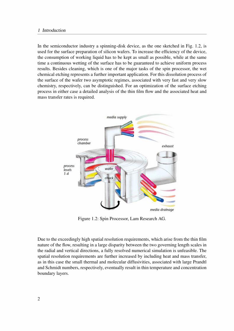
In the semiconductor industry a spinning-disk device, as the one sketched in Fig. 1.2, isused for the surface preparation of silicon wafers. To increase the efficiency of the device,the consumption of working liquid has to be kept as small as possible, while at the sametime a continuous wetting of the surface has to be guaranteed to achieve uniform processresults. Besides cleaning, which is one of the major tasks of the spin processor, the wetchemical etching represents a further important application. For this dissolution process ofthe surface of the wafer two asymptotic regimes, associated with very fast and very slowchemistry, respectively, can be distinguished. For an optimization of the surface etchingprocess in either case a detailed analysis of the thin film flow and the associated heat andmass transfer rates is required.
Figure 1.2: Spin Processor, Lam Research AG.
Due to the exceedingly high spatial resolution requirements, which arise from the thin filmnature of the flow, resulting in a large disparity between the two governing length scales inthe radial and vertical directions, a fully resolved numerical simulation is unfeasible. Thespatial resolution requirements are further increased by including heat and mass transfer,as in this case the small thermal and molecular diffusivities, associated with large Prandtland Schmidt numbers, respectively, eventually result in thin temperature and concentrationboundary layers.
2

1.1 Motivation
The complex physics which governs the flow results in a variously shaped free surface.Fig. 1.3 depicts the effect of an increase of the volumetric flowrate Q on the topology ofthe free surface. For moderate flow rates large scale wave structures can be observed inthe radially outer region, see Fig. 1.3a. As the volumetric flowrate is increased, these largescale structures tend to break up into small-scale, three-dimensional wave structures, seeFigs. 1.3b-1.3c. This highly irregular free surface, associated with complex wave dynam-ics, additionally challenges any numerical simulation of the flow.
(a) Q=0.36 lpm (b) Q=0.6 lpm (c) Q=1.2 lpm
Figure 1.3: Waves encountered on a spinning disk using a high-speed camera (2000 fps)considering a constant revolution speed of n=200 rpm and water as workingliquid. Exps. [2].
The present work attempts to analyze computationally the wavy thin film flow and theassociated heat and mass transfer characteristics on a spinning disk in order to describeand to investigate the salient features of the process of wet chemical surface etching in twoasymptotic regimes, associated with very fast and very slow chemistry.
3

1 Introduction
1.2 Review of previous work
Due to their high technical relevance and the complexity of the wave dynamics of the freesurface flow, thin film flows have been and are still subject of numerous specific papersand scientific monographs (e.g. Chang and Demekhin [3], Kalliadasis et al. [4]). Compre-hensive reviews on the dynamics of thin liquid films were presented by Oron et al. [5] andCraster and Matar [6].While thin films driven by centrifugal forces are attracting increasingly attention in variousengineering applications, due to the fact that the film thickness can be controlled by therotational speed, historically, most effort has been put into analyzing thin liquid films flow-ing under the action of gravity. For these films, which are falling down a vertical wall or aninclined plane, a wide variety of waves was found and classified in various experimentalstudies. Typical flow quantities, such as the thickness of the liquid film, have been mea-sured and the stability of the flow was analyzed. The modeling efforts of falling films canbe basically divided in mathematical models for systems with negligible and significantinertia, resulting in a lubrication approximation for the former, and an integral boundarylayer (IBL) approximation for the latter case.Thin film flows driven by centrifugal acceleration bear in many aspects close resemblanceto the falling film problem and many of the typical flow features apply to both cases. There-fore, for the sake of completeness, the present review starts with a section on falling liquidfilms, before it continues with thin liquid films driven by centrifugal forces.
1.2.1 Falling liquid films
In 1916 Nusselt [7] presented a steady-state base solution to the Navier-Stokes equationsfor a thin liquid film falling under the influence of gravity. This mathematically simplesolution, which is essentially represented by a semi-parabolic streamwise velocity profile,is often referred to as Nusselt flat-film solution. In real falling liquid films flow instabilitiesin general produce a wide variety of surface waves, as first analyzed experimentally byKapitza and Kapitza [8]. In a first analytical attempt to analyze the wave dynamics, thelinear stability of the Nusselt flat-film solution to small perturbations was studied by severalauthors (e.g., Benjamin [9], Yih [10]). Applying a classical Orr-Sommerfeld linear stabilityanalysis, the film was found to be unstable to long-wavelength disturbances above a criticalReynolds numberRecrit, due to inertial forces. The waves at the inception of the instabilitywere found to travel with twice the interface velocity. Benjamin [9] found the criticalReynolds number to be
Recrit =56
cot(θ) , (1.1)
with θ denoting the angle of inclination of the substrate. This correlation was confirmed inexperiments by Binnie [11, 12], whereas the experimental findings of Tailby and Portalski
4

1.2 Review of previous work
[13] on the stability of the film did not agree with Eq. (1.1). Wave inception on fallingfilms was shown to be a convective instability (Joo and Davis [14], Cheng and Chang [15]).Disturbances at the inlet are convected downstream, where they are amplified and triggersecondary instabilities. The linear theory is therefore only applicable in the inception re-gion. Additionally, the wave dynamics can be supposed to be very sensitive to upstreamflow noise, which is often hard to control.The extension of the stability analysis to the nonlinear regime was initiated by Benney [16],who presented a single evolution equation for the film thickness, known as Benney equa-tion. For small Reynolds numbers this equation describes the onset of waves correctly, butit fails in practically relevant settings with moderate Reynolds numbers, since it assumesonly a weak influence of inertia, which is on the other hand the key instability mechanism.In the limit of small amplitudes the Benney equation can be further reduced to an equationknown as Kuramoto-Sivashinsky equation. This type of equation is often found in nonlin-ear long-wave simplifications of the Navier-Stokes equations, and it has been extensivelystudied. So it was considered by Chang [17] and Yang [18] to analyze traveling waves onfalling films.For practically relevant cases from moderate to high Reynolds numbers, a method basedon a combination of the boundary-layer theory and the von Kármán-Pohlhausen integralapproximation has been widely used (Kapitza [19], Shkadov [20]). This approach, oftenreferred to as Shkadov model, leads to a coupled system of nonlinear hyperbolic partial dif-ferential equations for the film thickness and the instantaneous local flowrate. The systemof equations is solved for the depth-averaged flow variables assuming polynomial profilesfor the velocity variation inside the film. Wilkes and Nedderman [21] and Portalski [22]experimentally found that the streamwise velocity profile can be approximated reasonablywell by a second-order polynomial, even inside a wavy film.The equations of the Shkadov model are often referred to as integral-boundary-layer (IBL)equations. The solution of this nonlinear system of hyperbolic partial differential equa-tions, is basically non-unique. This implies that for a fixed wave frequency and fixed pro-cess parameters several sets of solutions can exist. These sets of solutions are called wavefamilies. The solutions in one family are categorized by the phase velocity and the heightof the wave peak. The different wave families were analyzed by Shkadov [20], Bunov etal. [23] and Sisoev and Shkadov [24]. Sisoev and Shkadov [25, 26] also introduced theconcept of dominating waves. These are attracting wave regimes, which are most likelyto be realized, independently of the initial conditions. The dominating waves were alsoshown to be the waves with the greatest velocity and the largest peak height in a family.Applying the concept of dominating waves, the predictions of the Shkadov model were ingood agreement with the experimental results of Alekseenko et al. [27].An improvement to the Shkadov model was presented in the work of Ruyer-Quil andManneville [28, 29]. They proposed a refined model for the flow inside the film by apply-ing the method of weighted residuals to expand the streamwise velocity field on a poly-nomial basis. Scheid et al. [30] carried out numerical simulations for a two-dimensionalformulation of this improved model in order to obtain solutions for three-dimensional film
5
1 Introduction
flow. In a comparison against results from a direct numerical simulation by Salamon etal. [31], very good agreement for several traveling-wave families was found. Malamatariset al. [32] found in a direct numerical simulation (DNS) of the Navier-Stokes equationssignificant deviations from a semi-parabolic shape, especially in the vicinity of large soli-tary waves. The weighted-residual integral-boundary-layer (WRIBL) model was provenas capable to reproduce even such velocity profiles. The numerical results of the WRIBLmodel were also compared against experimental results of Liu and Gollub [33], Liu etal. [34], Alekseenko et al. [27, 35] and Park and Nosoko [1]. Good qualitative agreementwas found and typical features, like herringbone and horseshoe shaped structures, couldbe reproduced.
Direct numerical simulations of the Navier-Stokes equations were considered by a num-ber of researchers to analyze the falling film problem without any model assumptions onthe velocity distributions inside the liquid. Malamataris et al. [36] and Salamon et al. [31]applied this computationally demanding approach and solved the governing set of equa-tions numerically with a finite-element method. In these studies, similar to the numericalstudy carried out by Jayanti and Hewitt [37], the upper boundary condition was imposedat the interface, so that the ambient air was not part of the solution. Gao et al. [38] carriedout a direct numerical simulation of the Navier-Stokes equations using the volume-of-fluid(VoF) method. They imposed a periodic forcing at the inlet to reproduce the experimentallyobserved wave structures. Small amplitude waves with sinusoidal-shape and a wave veloc-ity in close agreement with the experimental observations of Kapitza [39] were found. Forthe large amplitude waves, the experimentally observed tendency of these waves to inheritthe forcing frequency (Nosoko et al. [40]) was confirmed. Recirculation zones were foundinside very large amplitude waves, located inside a confined region beneath the peak ofthe surface. The velocity profiles inside the liquid film were analyzed and a good over-all agreement with the semi-parabolic analytical velocity profile was found in regions ofthe wave crests and slopes. In the wave troughs, however, where capillary ripples precedethe large amplitude waves, significant deviations from the semi-parabolic velocity pro-files were found. In this region also the pressure variation was found to be largest, as thestrong variation of the surface curvature translates into a strong variation of the capillarypressure.
Heat and mass transfer in falling films
Heat and mass transfer in falling films was also studied with considerable interest. A de-tailed review on modeling advances was, for example, presented by Yih [41]. Kapitza [39]proposed an approximate model to predict transfer coefficients in a wavy film to accountfor the experimentally observed intensifying effect of wavy flow on the transfer character-istics. The decrease of the average film thickness due to waviness of the surface was foundto provide a substantial contribution to the intensification of the heat and mass transferrates. Other modeling efforts were rather based on constant film thickness assumptions,
6
1.2 Review of previous work
which include an empirically determined eddy diffusivity to account for the intensifiedtransfer due to the waviness.Experimental investigations dealing with the heat transfer in falling liquid films (see, e.g.Kirkbride [42], Chun and Seban [43]) indicated an increase of the heat transfer coefficientover the steady-state Nusselt prediction. Hirshburg and Florschuetz [44, 45] used an in-tegral method to model the wavy thin film flow and the associated heat transfer based onthe semi-parabolic Nusselt profile and a linear approximation for the temperature profile.The results were found to be in good agreement with experimental data. In the numericalstudy of Miyara [46] the effect of local film thinning together with a convection effect ofcirculation flow in large amplitude waves was found to be responsible for the enhancementof the heat transfer coefficient in a falling wavy liquid film.As for the mass transfer especially the gas-liquid mass transfer across the film surfacehas received considerable attention. Emmert and Pigford [47] experimentally observedan enhancement of about a factor of 2.5 for the absorption of CO2 by water, as com-pared against theoretical predictions using the flat-film solution for the flow field. Solu-tions from an approximate model, in which a Kapitza-type velocity distribution was usedto solve the convection-diffusion equation (e.g. Ruckenstein and Berbente [48]), predictedenhanced transfer rates, but the obtained magnitude of the mass transfer coefficient wasstill smaller than the experimentally observed magnitude. Wasden and Dukler [49] used asemi-empirical model, in which the flow solution is constructed from experimental data,to solve the diffusion equation in a coordinate system moving with the wave. The resultsfor the absorption rates were in good agreement with the experimental findings. Sisoev etal. [50] modeled the gas absorption process in the presence of regular waves, by utilizingthe dominating wave solution to solve a two-dimensional convection-diffusion equation. Anumber of studies were also concerned with the solid-liquid mass transfer rates at the wet-ted substrate. Hirose et al. [51] analyzed the dissolution of solid material from the substrateunder laminar flow conditions experimentally and analytically. Analytical solutions wereobtained by introducing the semi-parabolic Nusselt flat-film profile for the streamwise ve-locity component. They found, that in the smooth regions of the flow, the predictions ofthe steady-flow model matched the experimental results well. For wavy flow an enhance-ment in the solid-liquid mass transfer process was found and the reduction of the meanfilm thickness was identified as main reason for this enhancement. Brauner and Moalem-Maron [52] observed by means of simultaneous measurements of the instantaneous filmthickness and the local transfer rate, a close correlation between the motion of the wavesand the local mass transfer. In the same study, the major enhancement effect was foundto be due to the large amplitude waves, where the transfer rates reached a local maximumbeneath the propagating front of the wave.
7

1 Introduction
1.2.2 Rotating films
Thin films driven by centrifugal forces bear resemblance to the problem of falling filmsin many aspects. The main differences, which exacerbate the modeling of these flows,arise from the radially varying acceleration and the presence of the Coriolis force. Tocharacterize the flow it is therefore useful to consider the Rossby number Ro and theEkman number Ek, which rate the importance of the Coriolis force relative to the inertialand viscous forces, respectively. As shown by Rauscher et al. [53] at large radii r, wherethe thickness of the liquid film δ is sufficiently small, an asymptotic solution can be foundin terms of a series expansion of the Navier-Stokes equations. In the asymptotic limit oflarge radii the radial momentum equation is essentially governed by the balance of thecentrifugal and viscous forces. This balance can be written as
O(Ω2r
)∼O
(ν
Q
2πrδ3
), (1.2)
involving the volumetric flowrate Q and the kinematic viscosity ν of the fluid. It thenfollows that
νQ
2πΩ2r2δ3∼O (1) , (1.3)
which can be rewritten as the product of the local Ekman and the Rossby numbers(
ν
Ωδ2
)
︸ ︷︷ ︸Ek
(Q/2πrδrΩ
)
︸ ︷︷ ︸Ro
∼O (1) . (1.4)
Since the inertial forces become insignificant at very small Rossby numbers, Ro 1, theneglect of the inertial forces in the asymptotic limit, requires a sufficiently high Ekmannumber, so that
Ek ·Ro∼O (1) (1.5)
is satisfied. It immediately follows that the more the Ekman number exceeds unity theless effect have the inertial forces. At the same time, being defined as the ratio of the vis-cous forces to the Coriolis forces, a large Ekman number implies negligibly small Coriolisforces.From Eq. (1.4) it follows that the film thickness at large radii is proportional to
δ ∝
(1
2πQν
Ω2r2
)1/3
.
(1.6)
In this asymptotic limit, the centrifugal force term is driving the radial motion equivalentlythe gravitational force term in the Nusselt flat-film solution for falling liquid films.
8

1.2 Review of previous work
Based on the order of magnitude of the convective terms, which are O(Ro2) relative to
the leading order centrifugal term, and a length scale in vertical direction defined as
δ0 =( νΩ
)1/2, (1.7)
Rauscher et al. [53] suggested to introduce
l0 =
(9Q2
4π2νΩ
)1/4
(1.8)
for the characteristic radial length scale.
Experimental work
Experimental investigations on rotating films were mostly dedicated to the classification ofdifferent wave regimes and measurements of the local film thickness. The film thicknessmeasurements were carried out using either mechanical, optical or electrical measurementtechniques.
Espig and Hoyle [54] carried out the first systematic experimental investigation, utilizing aneedle probe method. They reported four different flow types, including uniformly smoothfilm flow, flow with concentric waves, and flow with helical waves. For wavy flow themaximum film thickness, corresponding to the amplitudes of the waves, was found to beup to 40% higher than the film height predicted by the Nusselt flat-film analogon, which isproportional to Eq. (1.6) with the constant of proportionality given as 31/3. This flat-filmanalogon was shown to represent the asymptotic solution of the boundary-layer equationsin the limit of small Rossby numbers, Ro 1, (Aroesty et al. [55]).Leshev and Peev [56] measured the film thickness using alternatively water or glycerol-water solutions to investigate the validity of the asymptotic solution. While the maximumfilm thickness for water was found to be significantly higher than predicted by the asymp-totic solution, there were only slight deviations for the higher viscous liquids, suggestingan attenuation of the waviness due to an increase of the viscosity.
While most mechanical methods constrain the film thickness measurements to the peakheight of the waves, optical or electrical methods allow to obtain the time-averaged meanfilm thickness. Charwat et al. [57] used an infrared-absorption technique to measure thelocal mean film thickness of water, a water-glycerin solution, and a number of alcoholson a rotating a disk made of optical glass. The measured film thickness was found to besignificantly lower than predicted by the asymptotic smooth-film solution. The smooth-film predictions exceeded the experimental results with a maximum deviation up to 50%.
9

1 Introduction
Based on their experimental data Charwat et al. [57] modified the exponent as well as thepre-factor of the asymptotic smooth-film solution to obtain the correlation
δ
r= 1.6
(Qν
Ω2r5
)0.4
, (1.9)
which provides the best fit to their film thickness measurements. Based on qualitative ob-servations they further distinguished three wave regimes, with concentric waves, spiralwaves, and irregular, wedge-like wavelets. Waveless flow was found only for small volu-metric flowrates and low rotational speeds. The speed of the concentric waves was foundto be a factor of 1.7-2.8 faster than the surface velocity of the smooth-film flow. The peakheight of the waves was found to be up to 50% higher than the local mean film thickness.
Woods [58] measured the intensity of light that passed through a dye impregnated waterfilm. This optical method allows for accurate measurements of the instantaneous shape ofthe wavy surface, see e.g., Fig. 1.4. The scaling used in Fig. 1.4 is based on the definitions(1.7) and (1.8), introduced as r= rl0, and δ= δδ0, as suggested by Rauscher et al. [53]. Theobserved waves were classified as two- or three-dimensional, and the peak height of thewaves was found to be very large, with a maximum of about four times the local mean filmthickness. This maximum occurred at a radial transition point, where the two-dimensionalwaves broke up into three-dimensional wavelets.Ozar et al. [59] utilized the reflection of laser-light from the free surface to determine the
location of the liquid-air interface. The inflow conditions were controlled by a co-rotatingcollar with fixed height and length. A local maximum in the film height was observedand identified as hydraulic jump. The radial position of the hydraulic jump was observedto depend on the rotational speed and a Reynolds number, which was defined using theinitial velocity of the liquid and the height of the film at the exit of the collar as velocityand length scales, respectively. Three flow-regions were distinguished: an inner, inertia-dominated region, a transition region and a rotation-dominated outer region. Wavy flowwith increasing wave amplitudes was observed with increasing Reynolds number.Thomas et al. [60] considered a similar experimental setup. The local mean film thicknesswas measured using a capacitance technique. They observed wavy flow, in the super- andsubcritical regions, before and after the hydraulic jump, respectively.
A non-intrusive technique was also used by Miyasaka [61], who focused on the radiallyinner flow region. In his experiments the change in the electrical resistance of a glycerin-solution was utilized to measure the film thickness with an accuracy of ± 0.01 mm. Thesame measurement principle was utilized by Muzhilko et al. [62], who found the mean filmthickness in the radially outer region to be about 20% less than predicted by the asymptoticsmooth-film solution.
10

1.2 Review of previous work
δ
r2.6 2.7 2.8 2.9 3 3.1
0.2
0.6
1
1.4
1.8
Figure 1.4: Instantaneous film thickness profile as obtained by Woods [58].Operating conditions Q=0.78 lpm, n=400 rpm and ν=1×10⁻⁶ m2/s.
Leneweit et al. [63] measured the velocity of the free surface. The film thickness was eval-uated by assuming, that the radial and azimuthal components of the velocity agree to theleading order terms with the asymptotic smooth-film solution. They investigated the evo-lution of spiral waves triggered by local perturbations at the entrance of the liquid. For lowflowrates, the wave velocity was found to be about twice the local surface velocity, whichis in accordance with predictions from the linear stability theory.Lim [64] used a microdensiometer technique to measure the local mean film thickness. Itwas found to be about 20% less than predicted by the asymptotic smooth-film solution andcorrelated in terms of two dimensionless groups.
Burns et al. [65] measured the time-averaged film thickness by utilizing the fact, that thefilm thickness is inverse proportional to the electrical resistance. The film thickness mea-surements were carried out for four different liquids and the results were found to be onaverage about 9% less than predicted by the asymptotic smooth-film solution. Three zoneswere identified, based on the occurrence of turning points in the radial velocity profile: aninjection zone, an acceleration zone, and a synchronized zone. An estimate for the radialextensions of the two inner, inertia dominated zones was proposed as well. In Fig. 1.5 theexperimental results of Burns et al. [65] are compared against the leading order term of theasymptotic solution, using the scaling quantities suggested by Rauscher et al. [53]. Theseresults illustrate the typical observations from experimental studies in which the local mean
11

1 Introduction
(h)
(g)
(f)
(e)
(e)
(c)
(b)
(a)
δ
r
0.5 1 2 3 40
1
2
Figure 1.5: Measurements of the film thickness by Burns et al. [65] for Q=1.80 lpm,ν=1.3×10⁻⁶ m2/s and (a) n=296 rpm, (b) n=401.1 rpm, (c) n=496.6 rpm, (d)n=601.6 rpm, (e) n=697.1 rpm, (f) n=802.1 rpm, (g) n=987.6 rpm, (h) leading-order term of asymptotic solution.
film thickness was analyzed. In the radially inner region, inertial effects dominate and theasymptotic solution is not valid. In the radially outer region the waviness of the film leadsto a lower local mean film thickness than predicted by the asymptotic far-field solution.
Numerical studies of rotating films
There exist only a few studies in which the film flow on the rotating disk is investigated byperforming detailed numerical simulations of the governing Navier-Stokes equations. Riceet al. [66] carried out a DNS assuming an axisymmetric flow field on an Eulerian mesh us-ing the VoF method to track the evolution of the two-phase flow field. They comparedtheir results for the film thickness against the experimental results of Thomas et al. [60]and Ozar et al. [59], where satisfactory agreement was found for the first, while overpre-dicted film heights were found for the latter.Rahman and Faghri [67] used a curvilinear boundary-fitted coordinate system for the nu-merical calculation of the three-dimensional flow in a pie-shaped slice of the disk. In theirapproach the free surface is used as an upper boundary of the computational domain, andtherefore the ambient gas was not part of the solution. In a comparison against experimen-
12

1.2 Review of previous work
tal data of Thomas et al. [60] a satisfactory agreement was found. The profiles of the radialvelocity component were assessed as well and found to be approximately semi-parabolic.Alike in the numerical study of Rice et al. [66], no waves were apparent, which is in con-trast to the experimental findings.
Kaneko et al. [68] performed an axisymmetric simulation using the VoF method to ana-lyze the flow on a spinning disk. They also included species transport in a binary mixtureto model the diffusion controlled process of wet chemical etching of silicon wafers. Thecomputational fluid dynamics (CFD) study was complemented by experiments, and the nu-merical predictions were found to be in good agreement with the experimentally observedetching rates.
Approximate models for rotating films
The mathematical modeling of films which are driven by centrifugal forces is closely re-lated to that of falling films. The concepts for providing approximate solutions for bothtypes of flow is therefore often based on the same methodologies. This affinity becomesobvious in the asymptotic solution of the boundary layer equations for large values of theradius. Applying the perturbation method using the dimensionless radius r = r/l0 as ex-pansion parameter, the leading order term of the radial velocity component resembles theNusselt smooth-film solution (Aroesty et al. [55]) with g replaced by Ω2r.Rauscher et al. [53] analyzed axisymmetric film flow on a spinning disk using an asymp-totic expansion in terms of r of the full Navier-Stokes equations, imposing free-surfaceboundary conditions on the liquid-gas interface. This series expansion yielded leadingzeroth-order terms of O
(r−1/3
)for the radial component of the velocity, which are iden-
tical to the smooth-film solution derived by Aroesty et al. [55].Needham and Merkin [69] used the method of matched asymptotic expansions and foundthat the asymptotic structure of the steady-state solution consists of an inner and an outerregion. In the inner region there is a rapid adjustment from the inlet conditions to the thinfilm regime, which can cause an increase of the film thickness. In the radially outer region,the film thickness is continuously decreasing. A linear stability analysis for the outer re-gion led to an instability criterion similar to the one obtained for the falling film problemby Benjamin [9], cf. Eq. (1.1),
Recrit =56, (1.10)
with a critical Reynolds number for the rotating film defined as Recrit = (QΩ2)/(2πgν).In this stability analysis the effect of surface tension was neglected.An analytical model for the linear stability of the rotating film was also presented byCharwat et al. [57]. In this model, which is only valid for large values of the radius and
13

1 Introduction
small wave numbers, the largest amplification factors were obtained for axisymmetric per-turbations, and the Coriolis force was shown to exert a stabilizing influence.Myers and Lombe [70] analyzed the applicability of the lubrication approximation to therotating thin film flow. They showed, that in the framework of the lubrication approxima-tion, which is based on the assumption that inertial forces are negligible, also the contri-butions from the Coriolis force will be negligible, since both terms appear in the radialmomentum equation with the same order of magnitude. When applying the lubrication ap-proximation (e.g. Emslie et al. [71], Momoniat and Mason [72]), a typical feature of therotating thin film flow is therefore omitted.
In most practically relevant settings and experimental studies the Ekman number is notlarge, so that the Coriolis force has to be considered. The theoretical analysis of rotat-ing films with finite Ekman numbers is mostly based on the thin film approximation,which leads to boundary-layer-type equations. Steady-state solutions of these boundary-layer equations were obtained numerically by Dorfman [73].
In a more popular approach, the IBL approximation, which essentially relies on the method-ology of the Shkadov falling-film model, is extended to the rotating disk problem. Accord-ingly, the von Kármán-Pohlhausen integral approximation is used to reduce the dimen-sionality of the problem. This method, which was for example considered by Miyasaka[61], leads to a coupled system of nonlinear hyperbolic partial differential equations forthe film thickness and the radial- and azimuthal flowrates. The reduction of the dimension-ality of the problem via depth-averaging requires assumptions for the profiles of the radial-and azimuthal velocity components. A popular choice for the profile of the radial veloc-ity component is a semi-parabola (e.g. Sisoev et al. [74]). This choice is motivated by thedominating balance between the viscous and the centrifugal forces at large radii, where aparabolic velocity profile is analytically obtained, but it has also a number of shortcomingsin the inner region. In the analysis of Kim and Kim [75] a quartic profile is therefore con-sidered instead, as this fourth-order polynomial properly accounts for the effect of inertiain the radially inner region. Due to the better representation of the inertial forces in the ra-dially inner region the results obtained using the IBL approximation with quartic velocityprofiles are generally in better agreement with results from numerical simulations of thefull Navier-Stokes equations, than the results obtained with an IBL approximation using aparabolic radial velocity profile. Sisoev et al. [74] and Kim and Kim [75] furthermore car-ried out a linear stability analysis of the IBL equations and found the wave lengths, phasevelocities, and amplification factors to be in good agreement with results obtained froman eigenvalue analysis of the linearized Navier-Stokes problem, which was carried out inthe work of Sisoev and Shkadov [76]. The stability analysis results obtained using the IBLapproximation with quartic velocity profiles (Kim and Kim [75]) also included the effectof surface tension, and were in better agreement with the results from the Navier-Stokesequations than those of Sisoev et al. [74]. For large radii and zero surface tension the insta-
14

1.2 Review of previous work
bility criterion of Needham and Merkin [69], see Eq. (1.10), was reproduced. Moreover,the leading order terms of a series expansion in r of the IBL equations for large radii wereshown to be nearly identical to the leading order terms of the asymptotic expansion of thefull Navier-Stokes equations.In the limit of large Ekman numbers, i.e. negligible Coriolis forces, the IBL equations forthe rotating disk problem reduce to those of the falling film (Shkadov [77]). Therefore,Sisoev et al. [78] considered in a first attempt the regular wave solutions of the fallingfilm problem to model waves on a rotating disk. The fairly good agreement of these quasi-steady periodic waves with experimental data of Woods [58] motivated an extension of theregular wave model to finite Ekman numbers. In this extended model (Sisoev et al. [74]) aproper scaling allowed a further truncation of the IBL equations yielding localized versionsof the IBL equations, where the flow is assumed to be locally homogeneous. A linear stabil-ity analysis of the localized IBL equations provided amplification factors, phase velocitiesand unstable wavelengths, which were close to results from the linearized Navier-Stokesproblem. It was therefore concluded, that the truncated equations comprise adequately thefeatures of the full problem. In order to obtain non-linear travelling wave solutions for thetruncated IBL equations, a corresponding non-linear eigenvalue problem was solved. Thedominating waves were compared against experimental data of Woods [58], where a verygood quantitative and qualitative agreement was found. The stabilizing influence of theCoriolis force in the axisymmetric wave regime was confirmed.Matar et al. [79] demonstrated that transient numerical solutions of the full IBL equa-tions exhibit finite-amplitude waves, whose wave structure is similar to the periodic, quasi-steady wave solutions from the bifurcation analysis of the localized model. Large ampli-tude waves, separated by long flat-film regions were observed. Furthermore they observeda coincidence between the maxima of the depth-averaged radial flow rates and the minimaof the depth-averaged azimuthal flowrates, so that the resulting Coriolis forces can effec-tively exert a stabilizing influence on the flow. Due to this retarding effect of the Coriolisforce, waves on falling films travel faster than waves on rotating films. Furthermore it wasshown, that with increasing effect of inertia the flow becomes more unstable.
Heat and mass transfer in rotating films
Experimental work
A number of experimental investigations were carried out with the focus on the heat andmass transfer in thin liquid films on rotating disks.Among these studies are the work of Ozar et al. [80], who proposed a correlation for thelocal Nusselt number. Aoune and Ramshaw [81] studied the local heat transfer rates be-tween the disk and the film. High heat transfer coefficients were found in the radially innerregion, which was supposed to be a thermal entrance effect. Also in the radially outer re-gion the heat transfer coefficients were found to be significantly higher than predicted bya simplified Nusselt smooth-film analysis.
15
1 Introduction
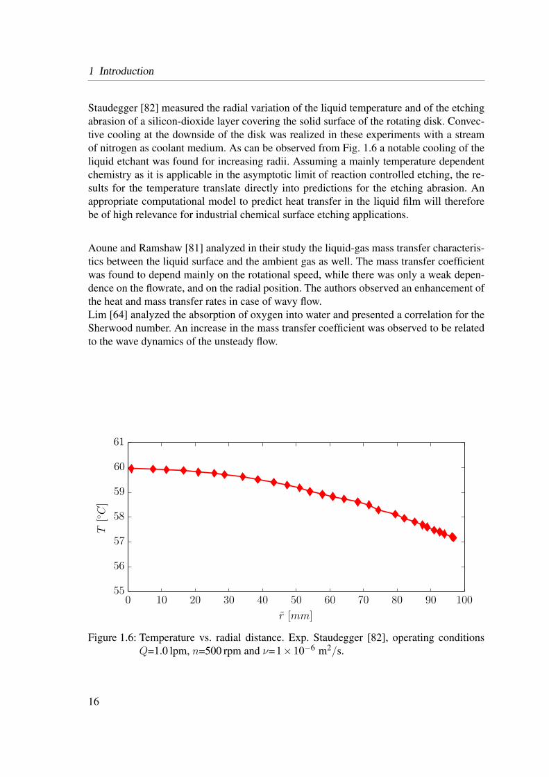
Staudegger [82] measured the radial variation of the liquid temperature and of the etchingabrasion of a silicon-dioxide layer covering the solid surface of the rotating disk. Convec-tive cooling at the downside of the disk was realized in these experiments with a streamof nitrogen as coolant medium. As can be observed from Fig. 1.6 a notable cooling of theliquid etchant was found for increasing radii. Assuming a mainly temperature dependentchemistry as it is applicable in the asymptotic limit of reaction controlled etching, the re-sults for the temperature translate directly into predictions for the etching abrasion. Anappropriate computational model to predict heat transfer in the liquid film will thereforebe of high relevance for industrial chemical surface etching applications.
Aoune and Ramshaw [81] analyzed in their study the liquid-gas mass transfer characteris-tics between the liquid surface and the ambient gas as well. The mass transfer coefficientwas found to depend mainly on the rotational speed, while there was only a weak depen-dence on the flowrate, and on the radial position. The authors observed an enhancement ofthe heat and mass transfer rates in case of wavy flow.Lim [64] analyzed the absorption of oxygen into water and presented a correlation for theSherwood number. An increase in the mass transfer coefficient was observed to be relatedto the wave dynamics of the unsteady flow.
T[C]
r [mm]
0 10 20 30 40 50 60 70 80 90 10055
56
57
58
59
60
61
Figure 1.6: Temperature vs. radial distance. Exp. Staudegger [82], operating conditionsQ=1.0 lpm, n=500 rpm and ν=1×10⁻⁶ m2/s.
16

1.2 Review of previous work
n = 1100 rpm
n = 900 rpm
n = 700 rpm
n = 500 rpm
R[µm/m
in]
r [mm]0 10 20 30 40 50 60 70 80 90 100
4
6
8
10
12
14
16
Figure 1.7: Etching rate profiles for various rotational speeds as obtained by Staudegger etal. [85]. Q=0.95 lpm and ν=2.87×10⁻⁶ m2/s.
The solid-liquid mass transfer on the disk was experimentally analyzed by Burns andJachuck [83], who utilized the limiting current technique for the process of copper de-position on a spinning disk. They observed an increase of the mass transfer coefficient incase of wavy flow, which is in contrast to the experimental findings of Peev et al. [84]. Inthe latter study the dissolution of a rotating gypsum disk was analyzed and the waviness ofthe liquid film was found to show no significant influence on the solid-liquid mass transferprocess.
Staudegger et al. [85] and Kaneko et al. [68] analyzed the etching activity of an aqueoussolution, consisting of nitric and hydrofluoric acid, flowing over a rotating silicon disk.This process is of high relevance for the semiconductor industry, where it is used for thethinning of silicon wafers, allowing for silicon chips with reduced thickness. As the chem-ical etching of silicon is mainly controlled by the convection-dominated mass transfer ofthe primary etchant component from the bulk liquid to the surface of the silicon wafer, itis essentially determined by the convection based solid-liquid mass transfer coefficient.Fig. 1.7 shows typical etching rate profiles for various rotational speeds as obtained byStaudegger et al. [85]. The largest etching rates are observed at the center of the disk,corresponding to the stagnation region of the impinging liquid jet. In this region the etch-ing rates are observed to be nearly unaffected by the rotational speed. Radially furtherdownstream a local maximum, with a radial position depending on the rotational speed,
17

1 Introduction
was observed. At larger radii the etching rates decrease. For the higher rotational speedsthe etching rates in the radially outer region show a constant or even slightly increasingbehavior. Staudegger et al. [85] additionally analyzed the influence of an increase of thevolumetric flowrate and different etchant temperatures on the etching rates. It was foundthat an increase of the rotational speed, as well as an increase of the volumetric flowrateand an increase of the etchant temperature led in general to higher etching rates. A qual-itative correlation between the observed etching rates and the corresponding approximateradial velocity profiles was obtained by considering an approximate two-parameter modelfor the steady-state smooth-film flow over the rotating disk.
Theoretical and computational work
Most previous theoretical work on the heat and mass transfer characteristics of the thinfilm flow on a spinning disk is based on the steady-state smooth-film solution of the flowfield in the asymptotic limit of large radii.
Aoune and Ramshaw [81] extended the Nusselt solution obtained for the film condensationin a falling film (Nusselt [7]) to the rotating film problem. The predictions of this simplifiedmodel were compared against their experimental data. For highly viscous liquids the ex-perimental results for the heat transfer were in satisfactory agreement with the predictionsfrom the simplified Nusselt analysis. Significant deviations were observed, when waterwas used as liquid, suggesting an attenuation of the waviness due to an increase of theviscosity. Additionally, the penetration model of Higbie (Higbie [86]) was applied, to pre-dict the liquid-gas mass transfer coefficient. Using this simple model the magnitude of theexperimentally obtained mass transfer coefficient was significantly underpredicted.
Basu and Cetegen [87] applied a thin film approximation combined with the von Kármán-Pohlhausen method to analyze the thermal characteristics of a heated film flow, assumingalternatively a constant disk temperature, as well as a constant heat flux as thermal bound-ary condition on the surface of the rotating disk. They did not account for the influence ofthe Coriolis force, as the momentum equation in azimuthal direction was not considered.The thermal entry length was neglected as well. Their obtained steady-state results exhibitdecreasing Nusselt numbers with increasing radii and a comparison against experimen-tal results of Ozar et al. [80] and numerical results of Rice et al. [66] showed reasonableagreement in the radially outer region.
Peev et al. [84] applied a method, known as method of Leveque (see, e.g., Bird et al. [88]),to analyze the solid-liquid mass transfer coefficient. In this method, which was also utilizedby Burns et al. [83], the concentration boundary layer is assumed to be very thin, implying
18

1.2 Review of previous work
a very large Schmidt number, so that the profile of the radial velocity inside this thin layeris approximately linear. The resulting simplified convection-diffusion equation can then besolved analytically in terms of Gamma functions. The predictions of this approximate dif-fusion model were compared against the experimental results of Peev et al. [84], as well asagainst the experimental results of Burns et al. [83]. While in the former case, satisfactoryagreement was found, the experimentally obtained mass transfer coefficient of the lattercase was significantly underpredicted.
Rahman and Faghri [89] presented a steady-state analytical solution for the gas absorptionat the gas-liquid interface and the solid dissolution at the disk surface. In their approachthe radial convection velocity is prescribed using the semi-parabolic profile obtained forthe steady-state smooth-film. The resulting convection-diffusion equation was cast in di-mensionless form and solved using a separation of variables, yielding solutions for thedimensionless concentration in terms of confluent hypergeometric functions. The resultsindicated a downstream increase of the mean bulk concentration, for the case of gas ab-sorption, as well as for the case of solid dissolution, as mass is diffused into the fluid.The Sherwood number was found to decrease with increasing radii due to the develop-ing concentration boundary layer. The results of this asymptotic analysis were comparedagainst their results from a fully three-dimensional numerical simulation (Rahman andFaghri [67, 89]), in which a curvilinear boundary-fitted coordinate system was used forthe numerical calculation of the three-dimensional flow in a pie-shaped slice of the disk.Assuming the free surface as upper boundary of the computational domain the ambientgas was not part of the solution. A good agreement between the numerical results and theanalytical solution was found in the radially outer region. In the radially inner region theanalytical solution did not produce satisfactory predictions, since inertial effects, which areneglected in the far-field solution, dominate. From the numerical results a local minimumin the Sherwood number was found in the radially inner region, where a maximum in thefilm thickness was observed.
A rather few number of previous analytical and numerical studies scrutinized the effect ofwavy flow on the heat and mass transfer characteristics. Sisoev et al. [90] solved a two-dimensional convection-diffusion equation in the framework of the localized IBL equa-tions. Although the wave profiles were assumed to be frozen in the numerical solutionof the convection-diffusion equation for the gas concentration, the obtained results indi-cated an enhancement of the rate of absorption due to the presence of the localized waves.This enhancement could be attributed to the deformation of the diffusion boundary layer,which increases the gas flux into the film. It was shown, that the local mass transfer ratesstrongly depend on the wave regimes, and therefore, for given process parameters (i.e.fixed Reynolds and Schmidt numbers), on the wave frequency. This finding attaches valueto a possible frequency forcing at the inlet, which can be of high relevance in industrial
19

1 Introduction
applications, when it comes to maximizing the transfer rates.
Matar et al. [91] solved for the full set of the unsteady IBL equations, where they alsoincluded a convection-diffusion equation for the concentration of the gas phase which isabsorbed into the film. The necessary closure relation was provided by adopting a com-posite profile function for the dissolved gas concentration. A single evolution equation forthe thickness of the concentration boundary layer and the base concentration is separatelysolved for both variables, since their total directional derivatives appear to be alternatelyzero, as it is dictated by the second law of thermodynamics. Numerical solutions for awide range of parameters were obtained using a finite-element method for the discretiza-tion in space and a linear multi-step method for the time integration. While in the radiallyinner region smooth film flow was observed, small-amplitude waves emerged in the outerradial region. Propagating further downstream these waves steepened and eventually coa-lesced forming large-amplitude waves, mostly preceded by capillary ripples. The observedwavy film surface translated into significant radial variations in the thickness of the con-centration boundary layer, and hence the local base concentration of the dissolved gas.On average, the base concentration was found to increase due to the presence of the non-linear waves. Their computational results for the averaged Sherwood number were alsocompared against the experimental data of Aoune and Ramshaw [81] showing good agree-ment. The limitations of steady-state models to describe heat and mass transfer rates werealso clearly demonstrated, as they are unable to capture any wave-induced enhancement ofthe transport.
1.3 Objectives of the present work
As it is outlined in the previous section the heat and mass transfer characteristics of thin liq-uid films on spinning disks were considered thus far only in a few theoretical and numeri-cal studies despite the high relevance of these transport phenomena for various engineeringapplications. Most of these previous studies investigate the heat transfer or the gas-liquidmass transfer characteristics in case of waveless smooth flow. Furthermore, most of thesestudies are restricted to large radii, where an asymptotic solution for the flow field can beobtained (cf. Rauscher et al. [53]) and the influence of the inertial and Coriolis forces isnegligible.
The present work attempts to extend the scope of these previous studies by covering thefull radial extension of the rotating disk including the inner and outer region, where it putsthe focus on the effect of unsteady wavy flow on the thermal conditions near the wall, aswell as on the solid-liquid mass transfer characteristics. As such this work is also intendedto provide essential input for the modeling of surface etching processes on a rotating wafer
20
1.4 Structure of the thesis
in the asymptotic wet chemical etching regimes, associated with very fast and very slowchemistry, respectively.The wavy thin film flow on a spinning disk at finite Ekman numbers shall be analyzed per-forming direct numerical simulations of the Navier-Stokes equations for a two-dimensional,axisymmetric flow field. The numerical analysis is based on the finite volume method, andthe volume of fluid method is used to track the free surface. As the DNS of the flow is toocostly for use as a computational design and optimization tool, the integral-boundary-layermethod, which is less laborious in terms of computational costs, and furthermore offersthe possibility for a straightforward extension to include heat and species mass transfer,is considered as an alternative approach. The predictive capability of the present IBL ap-proximation shall be assessed using the CFD results obtained from the DNS as well asexperimental measurements as reference data.
The main objectives of the present study are to
• computationally investigate the unsteady, wavy motion of the liquid film on the ro-tating disk based on CFD simulations and the IBL approximation,
• analyze the heat and species mass transfer between the disk and the liquid, with thefocus on the effect of waviness, as described by the IBL approximation, and
• model the surface etching process in the limit of large and small Damköhler numberson a rotating wafer.
1.4 Structure of the thesis
The present thesis is organized as follows:In Chapter 2, the governing equations are presented. The problem is parameterized bynon-dimensionalizing the governing equations using problem intrinsic scaling quantities.The thin film nature of the flow allows for a boundary-layer type approximation, whichconsiderably simplifies the governing equations. Solutions to the thin film equations forthe asymptotic case of very large Ekman numbers are reviewed and the integral boundarylayer equations for finite Ekman numbers are presented. The IBL method, which has so farbeen successfully used to analyze the fluid dynamics and gas absorption into a thin filmflow on a spinning disk, is then extended to model the heat transfer assuming a constantwall heat flux as thermal boundary condition, as well as to model the solid-liquid masstransfer in a binary mixture, assuming a constant species mass fraction at the wall. A sim-ple model to estimate the etching rates for wet chemical etching in the limit of large andsmall Damköhler numbers is presented.In Chapter 3 the numerical solution of the Navier-Stokes equations using the CFD sim-ulation software ANSYS FLUENT is outlined and some details regarding the description
21

1 Introduction
of the two-phase flow using the implemented VoF method are discussed. The numericalsolution procedure to solve the IBL equations, which comprise a hyperbolic system of par-tial differential equations, is based on a finite volume discretization and an approximateRiemann solver. The principles of Roe’s approximate Riemann solver are recalled, andsome details regarding the underlying wave-propagation theory, which provides flux lim-ited higher-order correction terms, are discussed.In Chapter 4 the results of the IBL model for the hydrodynamic, thermal and species masstransfer characteristics are presented and discussed starting with a detailed analysis of thesteady-state IBL results. The effects of wavy flow conditions on the time-averaged, as wellas on the instantaneous flow field and the heat and species mass transfer characteristicsare analyzed in detail. The predictions of the unsteady IBL model are assessed by compar-ison against results from CFD based numerical solutions of the Navier-Stokes equationsassuming axisymmetric flow. In addition to the comparison against numerical results thepredictive capability of the unsteady IBL model is also assessed by a comparison againstavailable experimental data. The validation distinguishes between two different regimesbased on the maximum values of the Ekman number which are reached at the outer radiusof the disk.In Chapter 5 the basic findings are summarized, and conclusions, as well as suggestionsfor further work are presented.
22

2 MATHEMATICAL MODELING AND APPROXIMATESOLUTIONS
2.1 Governing equations
The physical conservation laws of mass, momentum and energy provide the base for themathematical description of the flow and the associated heat and mass transfer. Additionalmaterial properties, which govern the flow and the heat and species mass transfer char-acteristics, as for example viscosity, surface tension, thermal conductivity, and moleculardiffusivity, are related to the nature of the fluid.The following overview gives a synopsis of the mathematical description following text-books on fluid mechanics, e.g. Batchelor [92], Spurk and Aksel [93], Kuhlmann [94],Pedlosky [95], or Baehr and Stephan [96].
Let ϕ(~x, t) represent the amount of some arbitrary physical property of a continuous ma-terial medium per unit volume. The total amount of this general physical field quantityϕ(~x, t) present in a finite volume V (t) is then obtained through the volume integral
∫
V (t)
ϕ(~x, t)dV. (2.1)
S0
V0−→n
−→v
Figure 2.1: Fluid material control volume.
23

2 Mathematical modeling and approximate solutions
The Reynolds transport theorem states that the rate of change of the total amount of ϕ(~x, t)within the material volume V (t), which is moving with the fluid velocity ~v, is given by
D
Dt
∫
V (t)
ϕdV =∫
V0
∂ϕ
∂tdV +
∫
S0
ϕ~v ·~ndS. (2.2)
Here the stationary volume V0, which is bounded by the surface ∂V0 ≡ S0, coincides withthe material volume V (t) at t= 0. The vector ~n denotes the outward pointing unit normalvector of the boundary S0, see Fig. 2.1.
2.1.1 Conservation of mass
In a continuum model the mass m present in a finite volume V is obtained through thevolume integral
m=∫
V (t)
ρ(~x, t)dV. (2.3)
Utilizing Reynolds transport theorem and replacing ϕ(~x, t) by the density ρ(~x, t), the con-servation of mass is stated as
Dm
Dt=∫
V0
∂ρ
∂tdV +
∫
S0
ρ~v ·d~S = 0, (2.4)
or alternatively, by applying the divergence theorem (see appendix 1), as
Dm
Dt=∫
V0
(∂ρ
∂t+∇ ·ρ~v
)dV = 0. (2.5)
The differential form of the continuity equation is obtained in the limit V0→ 0 as
∂ρ
∂t+∇ · (ρ~v) = 0. (2.6)
In a N -component system, the mass flux of the j-th species can be written as
~ηj = ρj~vj . (2.7)
Here the velocity of component j, denoted by ~vj , is defined relative to a stationary coordi-nate system. The total mass flux of the N -component system is then given by
~η =N
∑j=1
~ηj = ρ~v. (2.8)
24
2.1 Governing equations
The mass diffusion flux ~fj , defined relative to the motion of the mixture, reads
~fj = ρj (~vj−~v) . (2.9)
Incorporating the definition of the mass fraction c for component j
cj = ρj/ρ, (2.10)
the mass flux of species j can be decomposed into a diffusive flux ~fj and an overall flux ofthe mixture weighted with cj
~ηj = ~fj+ cjρ~v. (2.11)
The rate of change of species j in an arbitrary control volume Vj(t), moving with thespecies velocity ~vj is balanced by the rate of production of species j, denoted by Γj ,
D
Dt
∫
Vj
ρj dV =∫
Vj
Γj dV. (2.12)
Utilizing Reynolds transport theorem, Eq. (2.2), together with the divergence theorem, thedifferential form for the mass conservation in a N -component system, is obtained as
∂ρj∂t
+∇ · (ρj ~vj) = Γj . (2.13)
Employing the definition of the mass diffusion flux, Eq. (2.9), and assuming to the conti-nuity equation for a N -component system can be rewritten in terms of the species massfraction as
ρ∂cj∂t
+ρ~v ·∇cj =−∇ · ~fj+ Γj . (2.14)
In a two-component mixture with j = A,B, the diffusive flux ~fA is assumed to be wellapproximated by Fick’s law
~fA =−ρD∇cA. (2.15)
Considering a liquid with constant density and a constant coefficient of diffusion D, theconvection-diffusion equation for the species transport in a binary mixture is given by
∂cA∂t
+~v ·∇cA =D∇2cA+ ΓA/ρA. (2.16)
2.1.2 Conservation of momentum
The conservation of momentum states that the rate of change of momentum is equal to thetotal vector sum of the acting forces, written as
D~I
Dt= ~F . (2.17)
25

2 Mathematical modeling and approximate solutions
In a continuum model the momentum is defined as
~I =∫
V
ρ(~x, t)~v(~x, t)dV. (2.18)
The acting forces can be classified into long-range volume forces and short-range surfaceforces,
~F =∫
V
ρ~fB dV +∫
S
~τ dS. (2.19)
Therein the stress vector ~τ is defined as
~τ = ~n ·T, (2.20)
with the surface normal vector ~n and the stress tensor T. The conservation of momentumthen reads ∫
V0
∂ (ρ~v)
∂tdV +
∫
S0
ρ~v~v ·~ndS =∫
V0
ρ~fB dV +∫
S0
~τ dS, (2.21)
or alternatively by applying the divergence theorem∫
V
(∂ (ρ~v)
∂t+∇ · (ρ~v~v)
)dV =
∫
V
(ρ~fB+∇ ·T
)dV. (2.22)
In the present work only Newtonian fluids are considered. This implies a linear stress-strainrelation,
T =−p1+µ[
∇~v+(∇~v)T − 23(∇ ·~v)1
]+χ(∇ ·~v)1, (2.23)
with the dynamic viscosity µ and the volume viscosity χ. Furthermore the present anal-ysis is restricted to the flow of incompressible fluids with constant densities of all fluidsinvolved. Within such a framework the continuity equation, Eq. (2.6), reduces to
∇ ·~v = 0, (2.24)
and the stress tensor of Eq. (2.23) is given by
T =−p1+µ[∇~v+(∇~v)T
]. (2.25)
Rotating reference frame
For the mathematical modeling of thin liquid films on spinning disks, a reference framerotating with the disk’s angular speed Ω represents a natural choice. The conservation ofmomentum stated in Eq. (2.17) is only valid in an inertial frame of reference. In order to
26

2.1 Governing equations
describe the rate of change of an arbitrary vector in a rotating reference frame correctly, anextra term, which accounts for the time derivatives of the rotating unit vectors, has to beadded. The rate of change of an arbitrary vector ~s for an observer in an inertial referenceframe is given by (
D~s
Dt
)
I
=
(D~s
Dt
)
R
+ ~Ω×~s. (2.26)
Therein the first term on the right hand side (RHS) is the rate change of ~s as seen by anobserver in the rotating reference frame, and the second term gives the rate of change of theunit vectors of the rotating reference frame as seen by an observer in the inertial referenceframe. The velocity in the inertial reference frame, ~vI = (D~x/Dt)I , can be decomposedinto the sum of the velocity of the origin of the rotating reference frame ~vO, the relativevelocity in the rotating reference frame ~vR = (D~x/Dt)R, and the circumferential velocityΩ×~x,
~vI = ~vO+~vR+ ~Ω×~x. (2.27)
The acceleration in the inertial frame of reference is
(D~vIDt
)
I
=
(D~vODt
)
I
+
(D~vRDt
)
I
+
D(~Ω×~x
)
Dt
I .
(2.28)
Using Eq. (2.26) the total change of the relative velocity can be rewritten as(D~vRDt
)
I
=
(D~vRDt
)
R
+ ~Ω×~vR. (2.29)
Denoting the acceleration of the origin of the rotating system with ~aO = (D~vO/Dt)I , andrewriting the rightmost term in Eq. (2.28) using again Eq. (2.26) the acceleration in theinertial frame can be rewritten in terms of the rotating reference quantities
(D~vIDt
)
I
= ~aO+
(D~vRDt
)
R
+ 2 ~Ω×~vR︸ ︷︷ ︸Coriolis acc.
+ ~Ω×(~Ω×~x
)
︸ ︷︷ ︸centrifugal acc.
+d ~Ω
dt×~x
︸ ︷︷ ︸Euler acc.
. (2.30)
Considering only a non-moving origin, i.e. ~aO = ~0, three additional forces, which arisefrom the motion of the reference frame itself, have to be account for. These are the Cori-olis force, the centrifugal force, and the Euler force. Accordingly, the conservation of mo-mentum for an incompressible Newtonian fluid in a reference frame rotating with constantangular velocity Ω is given by
ρ
[∂~vR∂t
+(~vR ·∇)~vR+2 ~Ω×~vR+ ~Ω×(~Ω×~x
)]=−∇p+µ∇
2~vR+ρ~g. (2.31)
27

2 Mathematical modeling and approximate solutions
It should be noted here, that the continuity equation (2.24) has the same form in the inertialand the rotating reference frame,
∇ ·~vI = ∇ · (~vR+Ω×~x) = ∇ ·~vR = 0, (2.32)
since the divergence of the curl is identical zero.Rewriting the left hand side (LHS) of the convection-diffusion equation (2.16), as
∂cA∂t
+(~vR+ ~Ω×~x
)·∇cA =
[∂
∂t+(~Ω×~x
)·∇]cA+ ~vR ·∇cA
=
(∂cA∂t
)
R
+ ~vR ·∇cA, (2.33)
it is clear, that it remains in the same form as Eq. (2.16), when rewritten in terms of therelative velocity vR, using the time derivative, as well as the spatial operator ∇ relative tothe rotating frame.Since in the following a rotating coordinate system is always used as reference frame, therelative velocity vR is denoted by v, for reasons of readability.
2.1.3 Conservation of thermal energy
The conservation of thermal energy is considerably simplified when the fluid is assumedto be incompressible and Newtonian with constant thermal conductivity λ and constantheat capacity cp. Assuming furthermore only conductive heat flux q, which is described byFourier‘s law
q =−λ∇T, (2.34)
the conservation of thermal energy can be rewritten as a convection-diffusion equation forthe temperature T ,
∂T
∂t+~v ·∇T = a∇
2T. (2.35)
Here a denotes the thermal diffusivity defined as
a=λ
ρcp. (2.36)
28

2.1 Governing equations
2.1.4 Non-dimensionalization of the governing equations
The liquid film flow and the associated heat and species mass transfer for an incompressibleNewtonian liquid with constant fluid properties in a reference frame rotating with the disksangular speed Ω, are governed by the following system of partial differential equations
∇ ·~v = 0, (2.37)
∂~v
∂t+(~v ·∇)~v =−1
ρ∇p− ~Ω×
(~Ω×~x
)−2 ~Ω×~v+ν∇
2~v+~g, (2.38)
∂T
∂t+~v ·∇T = a∇
2T, (2.39)
∂c
∂t+~v ·∇c=D∇
2c. (2.40)
Therein, the body force due to gravity, ~fB =~g, is accounted for, while chemical reactions,as well as heat sources and dissipation are considered to be negligible.
The problem is considered in a cylindrical coordinate system with base vectors (~er, ~eφ, ~ez).The angular velocity vector is aligned with ~ez and is represented by ~Ω = (0,0,Ω)T . Thebody force vector reads ~g = (0,0,−g)T , and the position vector is given by ~x= (r, φ, z)T .The individual components of the velocity vector are denoted by ~v = (u, v, w)T .
The Coriolis term from the momentum equation (2.38) becomes
2 ~Ω×~v =
−2vΩ2uΩ
0
, (2.41)
and the centrifugal term is
~Ω× ( ~Ω×~x) =
−rΩ2
00
. (2.42)
To parameterize the problem the governing equations are non-dimensionalized, using thecharacteristic scaling quantities suggested by Rauscher et al. [53]. These scaling quantities
29
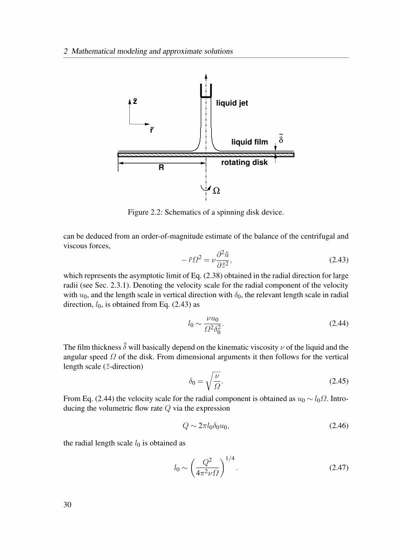
2 Mathematical modeling and approximate solutions
δ
liquid jet
liquid film
rotating disk
Ω
R
z
r
~
~~
Figure 2.2: Schematics of a spinning disk device.
can be deduced from an order-of-magnitude estimate of the balance of the centrifugal andviscous forces,
− rΩ2 = ν∂2u
∂z2 , (2.43)
which represents the asymptotic limit of Eq. (2.38) obtained in the radial direction for largeradii (see Sec. 2.3.1). Denoting the velocity scale for the radial component of the velocitywith u0, and the length scale in vertical direction with δ0, the relevant length scale in radialdirection, l0, is obtained from Eq. (2.43) as
l0 ∼νu0
Ω2δ20. (2.44)
The film thickness δ will basically depend on the kinematic viscosity ν of the liquid and theangular speed Ω of the disk. From dimensional arguments it then follows for the verticallength scale (z-direction)
δ0 =
√ν
Ω. (2.45)
From Eq. (2.44) the velocity scale for the radial component is obtained as u0 ∼ l0Ω. Intro-ducing the volumetric flow rate Q via the expression
Q∼ 2πl0δ0u0, (2.46)
the radial length scale l0 is obtained as
l0 ∼(
Q2
4π2νΩ
)1/4
. (2.47)
30
2.1 Governing equations
Rauscher [53] introduced an extra factor of 91/4, yielding the length scale into the radialdirection as
l0 =
(9Q2
4π2νΩ
)1/4
, (2.48)
which is used in the present work as well. The velocity scales v0 and w0 for the azimuthaland the vertical components of the velocity, respectively, are obtained from an order-of-magnitude analysis of the continuity equation. They are obtained as
v0 = u0, (2.49)
and
w0 =Ωδ0. (2.50)
The pressure scale is taken to be
p0 = ρΩ2l20, (2.51)
and the timescale is given by
t0 = l0/u0 = 1/Ω. (2.52)
The heat transfer is investigated assuming a constant wall heat flux boundary condition atthe surface of the spinning disk. Accordingly, a dimensionless temperature, which is basedon the constant heat flux prescribed at the wall, qw, and the given inflow temperature of theliquid Ti, is introduced as
θ =λ
qwδ0(T −Ti) . (2.53)
The solid-liquid mass transfer in a binary mixture is analyzed considering a constantspecies mass fraction equal to zero, cw = 0, at the wall. In the present scaling the con-stant inflow species mass fraction, ci, is used as reference quantity
c=c
ci. (2.54)
Introducing the characteristic scales given by Eqs. (2.45), (2.48)-(2.52), the non-dimen-sionalized Navier-Stokes equations read
1r
∂
∂r(ru)+
1r
∂v
∂φ+∂w
∂z= 0, (2.55)
∂u
∂t+u
∂u
∂r+v
r
∂u
∂φ+w
∂u
∂z− v
2
r=
− ∂p∂r
+2v+ r+∂2u
∂z2 + ε2[∂2u
∂r2 +1r
∂u
∂r+
1r2∂2u
∂φ− 2r2∂v
∂φ− u
r2
], (2.56)
31
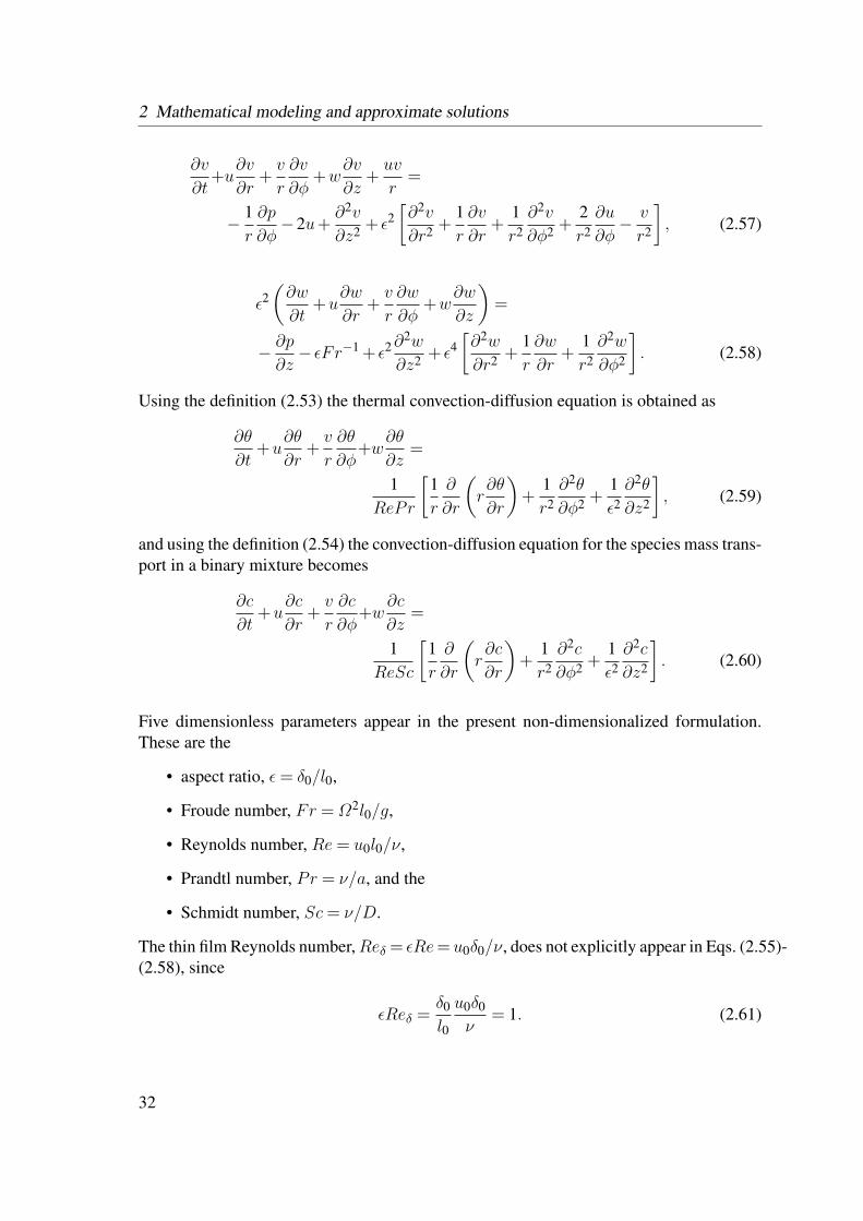
2 Mathematical modeling and approximate solutions
∂v
∂t+u
∂v
∂r+v
r
∂v
∂φ+w
∂v
∂z+uv
r=
− 1r
∂p
∂φ−2u+
∂2v
∂z2 + ε2[∂2v
∂r2 +1r
∂v
∂r+
1r2∂2v
∂φ2 +2r2∂u
∂φ− v
r2
], (2.57)
ε2(∂w
∂t+u
∂w
∂r+v
r
∂w
∂φ+w
∂w
∂z
)=
− ∂p∂z− εFr−1 + ε2∂
2w
∂z2 + ε4[∂2w
∂r2 +1r
∂w
∂r+
1r2∂2w
∂φ2
]. (2.58)
Using the definition (2.53) the thermal convection-diffusion equation is obtained as
∂θ
∂t+u
∂θ
∂r+v
r
∂θ
∂φ+w
∂θ
∂z=
1RePr
[1r
∂
∂r
(r∂θ
∂r
)+
1r2∂2θ
∂φ2 +1ε2∂2θ
∂z2
], (2.59)
and using the definition (2.54) the convection-diffusion equation for the species mass trans-port in a binary mixture becomes
∂c
∂t+u
∂c
∂r+v
r
∂c
∂φ+w
∂c
∂z=
1ReSc
[1r
∂
∂r
(r∂c
∂r
)+
1r2∂2c
∂φ2 +1ε2∂2c
∂z2
]. (2.60)
Five dimensionless parameters appear in the present non-dimensionalized formulation.These are the
• aspect ratio, ε= δ0/l0,
• Froude number, Fr =Ω2l0/g,
• Reynolds number, Re= u0l0/ν,
• Prandtl number, Pr = ν/a, and the
• Schmidt number, Sc= ν/D.
The thin film Reynolds number,Reδ = εRe=u0δ0/ν, does not explicitly appear in Eqs. (2.55)-(2.58), since
εReδ =δ0
l0
u0δ0
ν= 1. (2.61)
32

2.1 Governing equations
The boundary conditions for Eqs. (2.55)-(2.58) are no-slip conditions for the individualvelocity components on the disk’s surface and the kinematic boundary condition, as wellas the stress-free conditions on the free surface, which bring about a further dimensionlessparameter, a
• reduced inverse Weber number, W−1 = ε3We−1 = ε3 σρΩ2l0δ
20= 4π2σν3/2
9ρΩ3/2Q2.
The assumed hydrodynamic, thermal and species mass transport boundary conditions willbe discussed in more detail in the next section.
From Eqs. (2.59)-(2.60) the analogy between heat and species mass transfer is obvious.Accordingly, the solutions for the temperature and species mass fraction can be relatedthrough the ratio of the Schmidt to the Prandtl number. This ratio is represented by theLewis number
Le=a
D=Sc
Pr, (2.62)
which is basically defined as the ratio of the thermal to the molecular diffusivity. For unityLewis number, Le= 1, and identical non-dimensional boundary conditions Eqs. (2.59) and(2.60) would yield identical non-dimensional solutions for θ and c.
33

2 Mathematical modeling and approximate solutions
2.2 Thin film approximation
2.2.1 Governing equations and boundary conditions
Due to the thin film nature of the flow, the aspect ratio is small, ε 1, so that terms of orderO(ε2) and smaller are neglected, yielding a boundary layer type thin film approximationfor the flow on the spinning disk. In this limit the governing equations, Eqs. (2.55)-(2.60),reduce to
1r
∂
∂r(ru)+
1r
∂v
∂φ+∂w
∂z= 0, (2.63)
∂u
∂t+u
∂u
∂r+v
r
∂u
∂φ+w
∂u
∂z− v
2
r=−∂p
∂r+2v+ r+
∂2u
∂z2 , (2.64)
∂v
∂t+u
∂v
∂r+v
r
∂v
∂φ+w
∂v
∂z+uv
r=−1
r
∂p
∂φ−2u+
∂2v
∂z2 , (2.65)
0 =−∂p∂z− εFr−1, (2.66)
∂θ
∂t+u
∂θ
∂r+v
r
∂θ
∂φ+w
∂θ
∂z=
1Pr
∂2θ
∂z2 , (2.67)
∂c
∂t+u
∂c
∂r+v
r
∂c
∂φ+w
∂c
∂z=
1Sc
∂2c
∂z2 . (2.68)
The Reynolds number does not explicitly appear in Eqs. (2.67)-(2.68), since
1ε2Re
=l20δ2
0
ν
u0l0= 1. (2.69)
Incorporating the continuity equation (2.63) into the left hand sides of equations (2.64)-(2.68) and assuming the flow to be axisymmetric, the thin film equations can be rewritten
34
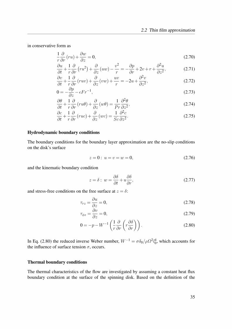
2.2 Thin film approximation
in conservative form as
1r
∂
∂r(ru)+
∂w
∂z= 0, (2.70)
∂u
∂t+
1r
∂
∂r
(ru2)+ ∂
∂z(uw)− v
2
r=−∂p
∂r+2v+ r+
∂2u
∂z2 , (2.71)
∂v
∂t+
1r
∂
∂r(ruv)+
∂
∂z(vw)+
uv
r=−2u+
∂2v
∂z2 , (2.72)
0 =−∂p∂z− εFr−1, (2.73)
∂θ
∂t+
1r
∂
∂r(ruθ)+
∂
∂z(wθ) =
1Pr
∂2θ
∂z2 , (2.74)
∂c
∂t+
1r
∂
∂r(ruc)+
∂
∂z(wc) =
1Sc
∂2c
∂z2 . (2.75)
Hydrodynamic boundary conditions
The boundary conditions for the boundary layer approximation are the no-slip conditionson the disk’s surface
z = 0 : u= v = w = 0, (2.76)
and the kinematic boundary condition
z = δ : w =∂δ
∂t+u
∂δ
∂r, (2.77)
and stress-free conditions on the free surface at z = δ:
τrz =∂u
∂z= 0, (2.78)
τφz =∂v
∂z= 0, (2.79)
0 =−p−W−1(
1r
∂
∂r
(r∂δ
∂r
)). (2.80)
In Eq. (2.80) the reduced inverse Weber number, W−1 = σδ0/ρΩ2l40, which accounts for
the influence of surface tension σ, occurs.
Thermal boundary conditions
The thermal characteristics of the flow are investigated by assuming a constant heat fluxboundary condition at the surface of the spinning disk. Based on the definition of the
35
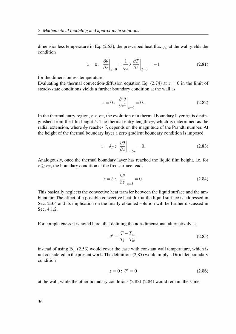
2 Mathematical modeling and approximate solutions
dimensionless temperature in Eq. (2.53), the prescribed heat flux qw at the wall yields thecondition
z = 0 :∂θ
∂z
∣∣∣∣z=0
=1qwλ∂T
∂z
∣∣∣∣z=0
=−1 (2.81)
for the dimensionless temperature.Evaluating the thermal convection-diffusion equation Eq. (2.74) at z = 0 in the limit ofsteady-state conditions yields a further boundary condition at the wall as
z = 0 :∂2θ
∂z2
∣∣∣∣z=0
= 0. (2.82)
In the thermal entry region, r < rT , the evolution of a thermal boundary layer δT is distin-guished from the film height δ. The thermal entry length rT , which is determined as theradial extension, where δT reaches δ, depends on the magnitude of the Prandtl number. Atthe height of the thermal boundary layer a zero gradient boundary condition is imposed
z = δT :∂θ
∂z
∣∣∣∣z=δT
= 0. (2.83)
Analogously, once the thermal boundary layer has reached the liquid film height, i.e. forr ≥ rT , the boundary condition at the free surface reads
z = δ :∂θ
∂z
∣∣∣∣z=δ
= 0. (2.84)
This basically neglects the convective heat transfer between the liquid surface and the am-bient air. The effect of a possible convective heat flux at the liquid surface is addressed inSec. 2.3.4 and its implication on the finally obtained solution will be further discussed inSec. 4.1.2.
For completeness it is noted here, that defining the non-dimensional alternatively as
θ? =T −TwTi−Tw
, (2.85)
instead of using Eq. (2.53) would cover the case with constant wall temperature, which isnot considered in the present work. The definition (2.85) would imply a Dirichlet boundarycondition
z = 0 : θ∗ = 0 (2.86)
at the wall, while the other boundary conditions (2.82)-(2.84) would remain the same.
36

2.2 Thin film approximation
Boundary conditions for the species transport
When considering the species transport in a binary mixture, the boundary conditions aregiven as
z = 0 : c= 0, (2.87)
and
z = 0 :∂2c
∂z2
∣∣∣∣z=0
= 0, (2.88)
at the wall, where the latter is obtained by evaluating the convection-diffusion equationEq. (2.75) at z = 0.
For large Schmidt numbers it is necessary to distinguish a concentration boundary layerwith thickness δc from the film height. In the region for r < rc, associated with a develop-ing concentration boundary layer, i.e. δc < δ, a zero-gradient upper boundary condition isimposed
z = δc :∂c
∂z
∣∣∣∣z=δc
= 0. (2.89)
Analogously, once the concentration boundary layer has reached the liquid film height, i.e.for r ≥ rc, the boundary condition at the free surface reads
z = δ :∂c
∂z
∣∣∣∣z=δ
= 0. (2.90)
It is noted that for unity Lewis number, Le= a/D= 1, the solution obtained for the speciesmass fraction c would be identical with the solution for non-dimensional wall temperaturefor the case with constant wall temperature defined by Eq. (2.85).
2.2.2 Far field asymptotic solution for Ek 1
As discussed in Sec. 1.2.2, an order-of-magnitude analysis yields in the limit of large radiithe expression
Ek ·Ro∼O (1) ,
which implies that for high Ekman numbers, Ek 1, the inertial, as well as the Coriolisforces are negligible. Assuming an axisymmetric and steady flow, far-field asymptotic so-lutions for the velocity and the film thickness can be analytically obtained in the case ofEk 1. Based on this far-field solution for the velocity, it is possible to obtain analyticalsteady-state solutions for the heat and mass transfer as well.
37

2 Mathematical modeling and approximate solutions
Asymptotic momentum balance
For large radii the radial momentum balance is governed only by the viscous and cen-trifugal forces. Thus, assuming the flow to be axisymmetric and steady, the asymptoticmomentum balance at large radii becomes
0 = r+∂2u
∂z2 , (2.91)
which is decoupled from the momentum equation into the azimuthal direction written as
0 =−2u+∂2v
∂z2 . (2.92)
Integration of Eq. (2.91), applying the boundary conditions of Eq. (2.76) and (2.78), andintroducing the rescaled wall normal coordinate ζ = z/δ, results in
u(r,ζ) = uδ(2ζ− ζ2) . (2.93)
The maximum velocity uδ is reached at the free surface (ζ = 1), and it is related to themean radial velocity by
u=1δ
δ∫
0
udz =23uδ. (2.94)
The semi-parabolic velocity profile given by Eq. (2.93) represents an exact asymptoticsolution in the limit of large radii, where the viscous and centrifugal forces dominate.Introducing the volumetric flowrate,
Q= 2rπδu, (2.95)
and recalling the length and velocity scales δ0, l0, and, u0 = l0Ω, specified in Eqs. (2.45)and (2.48), the substitution of Eq. (2.93) with uδ = (3/2)u due to (2.94) into Eq. (2.91)yields the following radial variation of the film thickness written in dimensional form
δ =
(3
2πQν
Ω2r2
)1/3
[m]. (2.96)
The asymptotic momentum balance for large radii into the azimuthal direction, Eq. (2.92),is governed by the balance between the viscous and the Coriolis forces. Integration ofEq. (2.92) using the parabolic profile for u as given by Eq. (2.93) leads to the quarticpolynomial
v(r,ζ) = vδ
(85ζ− 4
5ζ3 +
15ζ4). (2.97)
38

2.2 Thin film approximation
The mean velocity into the azimuthal direction is then obtained as
v =1δ
δ∫
0
vdz =1625vδ, (2.98)
and the maximum velocity vδ, corresponding to the maximum tangential slip, is reachedat the free surface, where ζ = 1.
Asymptotic higher-order expansion
Based on the far-field solution δ = r−2/3 for the film thickness, Rauscher et al. [53] intro-duced the similarity variable η as
η =z
δ=
z
δ0r2/3, (2.99)
so that the radial component of the flow velocity, Eq. (2.93), expressed in terms of η isgiven by
u= u0r−1/3
(η− 1
2η2). (2.100)
To obtain higher-order terms of the asymptotic solution for the axisymmetric flow-field,Rauscher reformulated the Navier-Stokes equations together with the corresponding bound-ary conditions in terms of η and r = r/l0, and obtained the following higher-order expan-sions in terms of r
δ = r−2/3 +
(62
315− 2
9εFr−1
)r−10/3 +O(r−4), (2.101)
u=13r−1/3− 1
3
(62
315− 2
9εFr−1
)r−3 +O(r−11/3), (2.102)
v =− 415r−5/3−
(115614175
− 8135
εFr−1)r−13/3 +O(r−5). (2.103)
Far-field solutions for the solid-liquid mass transfer
Based on the asymptotic solution for the flow field it is possible to obtain an analyticalsolution for species mass transfer as well. Rahman and Faghri [89], for example, presentedan analytical solution for species transport in case of solid dissolution at the disk surface.Neglecting convection into the vertical direction the asymptotic momentum and speciestransport equations (r 1) are given by
∂2u
∂z2 =−Ω2r
ν, (2.104)
39
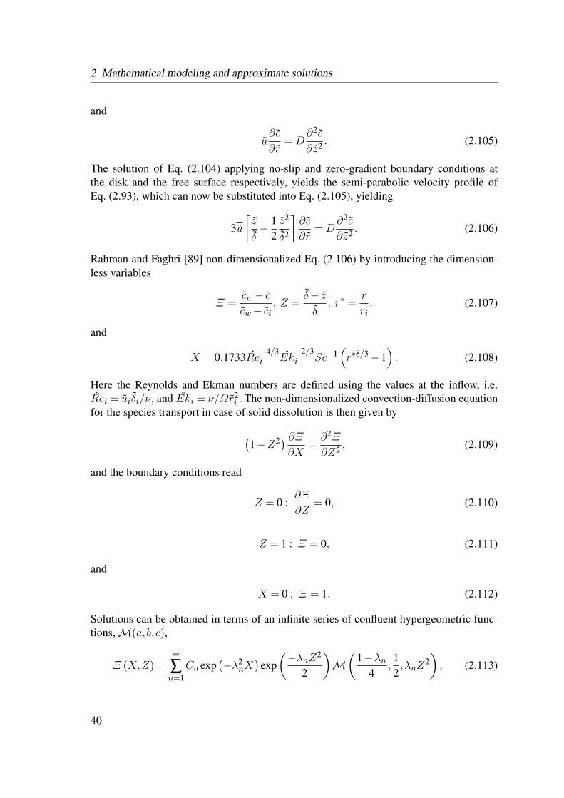
2 Mathematical modeling and approximate solutions
and
u∂c
∂r=D
∂2c
∂z2 . (2.105)
The solution of Eq. (2.104) applying no-slip and zero-gradient boundary conditions atthe disk and the free surface respectively, yields the semi-parabolic velocity profile ofEq. (2.93), which can now be substituted into Eq. (2.105), yielding
3u[z
δ− 1
2z2
δ2
]∂c
∂r=D
∂2c
∂z2 . (2.106)
Rahman and Faghri [89] non-dimensionalized Eq. (2.106) by introducing the dimension-less variables
Ξ =cw− ccw− ci
, Z =δ− zδ
, r∗ =r
ri, (2.107)
and
X = 0.1733Re−4/3i Ek
−2/3i Sc−1
(r∗8/3−1
). (2.108)
Here the Reynolds and Ekman numbers are defined using the values at the inflow, i.e.Rei = uiδi/ν, and Eki = ν/Ωr2
i . The non-dimensionalized convection-diffusion equationfor the species transport in case of solid dissolution is then given by
(1−Z2) ∂Ξ
∂X=∂2Ξ
∂Z2 , (2.109)
and the boundary conditions read
Z = 0 :∂Ξ
∂Z= 0, (2.110)
Z = 1 : Ξ = 0, (2.111)
and
X = 0 : Ξ = 1. (2.112)
Solutions can be obtained in terms of an infinite series of confluent hypergeometric func-tions,M(a,b,c),
Ξ (X,Z) =∞
∑n=1
Cn exp(−λ2
nX)
exp(−λnZ2
2
)M(
1−λn4
,12,λnZ
2), (2.113)
40
2.2 Thin film approximation
as shown by Rahman and Faghri [89], who present in their study the first 15 values of theeigenvalues λn and coefficients Cn.
A number of authors, (see, e.g., Burns et al. [83], or Peev et al. [84]) considered a method,known as method of Leveque, to model the solid-dissolution on a spinning disk. In thismethod a linear approximation for the velocity profile is assumed, presuming a very thinconcentration boundary layer. The resulting approximate convection-diffusion equationreads
3zδu∂c
∂r=D
∂2c
∂z2 , (2.114)
which can be cast into dimensionless form using the dimensionless concentration
Ξ = 1−Ξ =c− cicw− ci
(2.115)
and a similarity variable
η = z
(3uδ
19Dr
)1/3
= z
(Ω2δ
9Dν
)1/3
.
(2.116)
Applying the transformation into these new variables Eq. (2.114) becomes
d2Ξ
dη2 +3η2dΞ
dη= 0, (2.117)
with the boundary conditions
Ξ = 1 at η = 0, (2.118)
and
Ξ = 0 for η→ ∞. (2.119)
The solution of Eq. (2.117), is then obtained as
Ξ(η) = 1− γ(1
3 , η3)
Γ(1
3
) . (2.120)
Here
γ(a,x) =
x∫
0
ta−1e−tdt, (2.121)
denotes the incomplete gamma function, and
Γ (a) =
∞∫
0
ta−1e−tdt (2.122)
is the complete, or Euler, gamma function.
41
2 Mathematical modeling and approximate solutions
2.3 Integral boundary layer approximation
A popular approach for the analysis of rotating films with finite Ekman numbers is the IBLapproximation, in which depth-averaged quantities, defined by the integral average overthe film thickness
Υ =1δ
δ∫
0
Υ dz, (2.123)
are considered. The governing set of partial differential equations for the IBL model isobtained by averaging the thin film equations Eqs. (2.70)-(2.75) over the film thickness.
2.3.1 IBL approximation for hydrodynamics
Using the kinematic boundary condition Eq. (2.77), and considering the flow as axisym-metric, the depth-averaging of the continuity equation Eq. (2.70) yields
∂δ
∂t+
1r
∂
∂r
δ∫
0
rudz = 0, (2.124)
which can be written in terms of the depth-averaged velocity u as
∂δ
∂t+
1r
∂
∂r[ruδ] = 0. (2.125)
The integration of the thin film limit for the vertical component of the momentum equation,Eq. (2.73), yields an expression for the pressure written as
p= pδ+ εFr−1 (δ− z) . (2.126)
Here pδ denotes the pressure at the free surface, which can be computed from the stress-free boundary condition given by Eq. (2.80). The depth-averaged pressure is then obtainedas
p=1δ
δ∫
0
pdz = pδ+12εFr−1δ =
12εFr−1δ−W−1
(1r
∂
∂r
(r∂δ
∂r
)). (2.127)
42

2.3 Integral boundary layer approximation
Depth-averaging the radial component of the momentum equation, Eq. (2.71), yields
∂
∂t
δ∫
0
udz+1r
∂
∂r
δ∫
0
ru2 dz− 1r
δ∫
0
v2 dz =
− ∂
∂r
δ∫
0
pdz+pδ∂δ
∂r+ rδ+2
δ∫
0
vdz− ∂u
∂z
∣∣∣∣z=0
. (2.128)
Herein, the boundary condition Eq. (2.78) was used and again the kinematic boundarycondition Eq. (2.77) was applied to substitute the vertical component of the surface velocitywδ.Similarly, the depth-averaging of the azimuthal component of the momentum equation,Eq. (2.72), yields
∂
∂t
δ∫
0
vdz+1r
∂
∂r
δ∫
0
ruvdz+
δ∫
0
uv
rdz =−2
δ∫
0
udz− ∂v
∂z
∣∣∣∣z=0
. (2.129)
Rewriting the nonlinear convective fluxes in terms of
1δ
δ∫
0
u2 dz = kau2,
1δ
δ∫
0
uvdz = kbu v,
1δ
δ∫
0
v2 dz = kcv2, (2.130)
involving the profile constants ka, kb, kc, and introducing the expression
P = εFr−1δ−W−1(
1r
∂
∂r
(r∂δ
∂r
)), (2.131)
the depth-averaged continuity and momentum equations can be compactly rewritten as
∂
∂t
δδuδv
+
1r
∂
∂r
rδukar(δu)
2/δkbr(δu)(δv)/δ
= (2.132)
0kc(δv)
2/(rδ)+2(δv)+ b1(r− ∂P
∂r
)δ− b2(δu)/δ
2
−kb(δu)(δv)/(rδ)−2(δu)−5(δv)/(2δ2)
.
43

2 Mathematical modeling and approximate solutions
Therein, u, v are the depth-averages of the radial and azimuthal components of the ve-locity, respectively, and the constants b1 and b2 result from the derivatives of the radialand azimuthal components of the velocity at z = 0, appearing on the right hand side ofEq. (2.128) and Eq. (2.129). The depth-averaged continuity and momentum equations inEq. (2.132) are identical to the formulation obtained by Kim and Kim [75].
The reduction of the spacial dimensionality of the problem based on depth-averaging re-quires approximate assumptions for the profiles of the radial and azimuthal velocity com-ponents to compute the values of the profile constants ka, kb, kc, defined by Eq. (2.130), aswell as b1 and b2. The presently assumed profiles will be discussed in the following.
Profile assumptions
Radial velocity component
A popular choice for the profile of the radial component of the velocity is the semi-parabola(e.g. Sisoev et al. [74])
u(r,ζ) = uδ(2ζ− ζ2) , (2.133)
which is basically identical to the exact asymptotic solution in the limit of large radii,Eq. (2.93), where the viscous and centrifugal forces dominate (see Sec. 2.2.2). The second-order polynomial exhibits, however, a number of shortcomings in the radially inner region,where inertial and Coriolis forces are relevant. Therefore, the assumption of a quartic poly-nomial was proposed as an alternative (Kim and Kim [75]) written as
u(r,ζ) = uδ
(85ζ− 4
5ζ3 +
15ζ4)+κδ2
5ζ (1− ζ)2
(1− ζ
2
). (2.134)
This profile function introduces an additional profile parameter κ, which can be determinedfrom the radial momentum equation evaluated at z = 0,
∂2u
∂z2
∣∣∣∣z=0
=−r+ ∂p
∂r
∣∣∣∣z=0
:=−κ. (2.135)
Azimuthal velocity component
The azimuthal component of the velocity is approximated by the quartic polynomial (seeSec. 2.2.2)
v(r,ζ) = vδ
(85ζ− 4
5ζ3 +
15ζ4), (2.136)
which alike Eq. (2.133) represents an exact analytical solution obtained in the limit of largeradii.
44

2.3 Integral boundary layer approximation
Quadratic vs. quartic approximation
Substituting straightforwardly the quartic profile assumption Eq. (2.134) into Eq. (2.130)would result in very complex expressions for the integrations of the non-linear flux terms.It was therefore suggested by Kim and Kim [75] to compute the values of the profile con-stants ka, kb and kc using rather the quadratic approximation Eq. (2.133) for the radialcomponent of the velocity in the nonlinear integrands occurring in Eq. (2.130). The profileparameters b1 and b2 are still obtained using the quartic profile assumption Eq. (2.134).This approach is adopted in the present work as well, and it is referred to as quartic ap-proximation (IBL quart.) in the following. The profile constants used for the quartic andquadratic IBL approximation of the momentum equations are listed in Tab. 2.1.
profile parameter ka kb kc b1 b2IBL quad. 6/5 17/14 155/126 1 3IBL quart. 6/5 17/14 155/126 5/6 5/2
Table 2.1: Profile constants for the IBL approximation of the momentum equations.
Vertical velocity component
The profile of the vertical velocity follows implicitly from the assumptions for the othertwo velocity components to satisfy the continuity equation. Although the vertical veloc-ity profile is never needed in the solution of the depth-averaged equations, the insightinto the implicitly used w-profile can be helpful for the interpretation of the obtained IBLresults. Considering for example the quadratic radial velocity profile, Eq. (2.133), the pro-file for the vertical velocity component is obtained by integrating the continuity equation,Eq. (2.63), rewritten for axisymmetric flow
∂w
∂z=−1
r
∂
∂r
[ruδ
(z
δ− z
2
δ2
)]
.
(2.137)
Using the no-slip condition at z = 0 integration of Eq. (2.137) yields the third-order poly-nomial
w(r,z) =z3
δ3
(uδδ
3r− 2uδ
3∂δ
∂r+
13δ∂uδ∂r
)+z2
δ2
(−uδδ
r+uδ
∂δ
∂r− δ∂uδ
∂r
)
.
(2.138)
It can be shown that this w-profile satisfies the kinematic boundary condition, Eq. (2.77),by rewriting the depth-averaged continuity equation (2.125) assuming the quadratic u-profile, Eq. (2.133), associated with uδ = (3/2)u, as
∂δ
∂t=− 2
3r∂
∂r[ruδδ] . (2.139)
45

2 Mathematical modeling and approximate solutions
Using (2.139) it can be easily verified, that
wδ =∂δ
∂t+uδ
∂δ
∂r=−2
3δuδr− 1
3uδ∂δ
∂r− 2
3δ∂uδ∂r
, (2.140)
which is identical to the RHS of Eq. (2.138) evaluated at z = δ. Introducing the notation
aw(r) =−3ruδ ∂δ∂r
2ruδ ∂δ∂r +4δ(uδ+ r
∂uδ∂r
) , (2.141)
the profile for the vertical velocity component can be compactly rewritten as
w(r,ζ) = wδ
[ζ2(
32−aw(r)
)+ ζ3
(aw(r)−
12
)]
.
(2.142)
The depth-averaged vertical velocity is then obtained as
w = wδ
(38− aw(r)
12
)
.
(2.143)
The validity of this implicit assumption for the profile of the vertical component of thevelocity will be discussed in detail in Sec. 4.2.3.It should be noted here, that in case of steady-state smooth flow the vertical componentof the velocity tends to zero for large radii. This can easily be verified by substituting thefar-field solutions (r 1) for the film thickness δ = r−2/3, and the radial surface velocity,uδ =(1/2)r−1/3, into the asymptotic steady-state representation of the kinematic boundarycondition, Eq. (2.140), which yields
limr→∞
(wδ) = limr→∞
(uδdδ
dr
)≈ limr→∞
(2
3r2
)= 0, (2.144)
so that the vertical velocity profile given by Eq. (2.142) becomes identical zero.
2.3.2 IBL approximation for heat transfer
The thermal characteristics of the flow are investigated assuming a constant wall heat fluxboundary condition. Depth-averaging of the thermal convection-diffusion equation (2.74)and using the boundary conditions Eq. (2.81) and (2.84) yields
∂
∂t
δ∫
0
θdz+1r
∂
∂r
δ∫
0
ruθdz =1Pr
. (2.145)
46
2.3 Integral boundary layer approximation
To evaluate the integrals appearing on the LHS of the depth-averaged transport equationEq. (2.145), a profile assumption for the dimensionless temperature is required. For thispurpose a third-order polynomial ansatz function
θ(z) = a0 +a1z
δT+a2
z2
δ2T
+a3z3
δ3T
(2.146)
was chosen. Introducing the dimensionless wall temperature given as
θw = θ|z=0 , (2.147)
and using the boundary conditions Eqs. (2.81)-(2.82) together with Eq. (2.83), before thethermal boundary layer has reached the film surface (δT < δ), or, together with Eq. (2.84)thereafter (δT = δ), a composite profile for the dimensionless temperature is obtained as
δT < δ : θ =23δT + δT
(13z3
δ3T
− z
δT
), (2.148)
δT = δ : θ = θw+ δ
(13z3
δ3 −z
δ
). (2.149)
In the thermal entry region, r < rT , associated with δT < δ, the non-dimensional walltemperature is directly related to the thickness of the thermal boundary layer as
δT < δ : θw =23δT . (2.150)
Since the film in the radially inner region generally remains smooth, steady-state condi-tions are assumed within the thermal entry zone 0 < r < rT . Using the composite profilefunction given by Eqs. (2.148)-(2.149) produces the following expression for the depth-averaged temperature
θ =1δ
δ∫
0
θdz =
14δ2Tδ for δT < δ,
θw− 512δ for δT = δ.
(2.151)
The integration of the convective heat transport term uses for simplicity again only thequadratic profile assumption of the radial velocity u given by Eq. (2.133), which yields
1δ
δ∫
0
uθdz =
u
120δ3Tδ3 (24δ−5δT ) for δT < δ,
θwu− 61120δu for δT = δ.
(2.152)
Incorporating these expressions into the approximation for the transport of heat Eq. (2.145)yields evolution equations for the thickness of the thermal boundary layer δT < δ
∂
∂t
(δ2T
4
)+
1r
∂
∂r
[ruδ
(δTδ
)3(15δ− 1
24δT
)]=
1Pr
(2.153)
47

2 Mathematical modeling and approximate solutions
within the thermal entry region r < rT , and further downstream, when δT = δ, for the thedimensionless wall temperature θw,
∂
∂t
(δθw−
512δ2)+
1r
∂
∂r
(rδuθw−
61120
rδ2u
)=
1Pr
. (2.154)
2.3.3 IBL approximation for species mass transfer
Depth-averaging the species mass fraction convection-diffusion equation (2.75) and usingthe boundary condition Eq. (2.90) yields
∂
∂t
δ∫
0
cdz+1r
∂
∂r
δ∫
0
rucdz =− 1Sc
∂c
∂z
∣∣∣∣z=0 .
(2.155)
The necessary closure for the solution of the depth-averaged convection-diffusion equationcan be provided by choosing a third-order polynomial ansatz function for the profile ofspecies mass fraction c, generally written as
c
cδ(r)= a0 +a1
z
δc+a2
z2
δ2c+a3
z3
δ3c. (2.156)
Here δc denotes the thickness of the concentration boundary layer, and cδ = c|z=δ denotesthe value of c at the surface, which is constant in the region r < rc, where the concentrationboundary layer is distinguished from the film thickness. Accordingly, the surface value cδequals unity before the concentration boundary layer has reached the film surface (δc < δ),and varies with the radial position further downstream,
cδ =
1 δc < δ
cδ(r) δc = δ.(2.157)
The coefficients of the third-order polynomial are evaluated from the boundary conditionsEqs. (2.87)-(2.90), so that Eq. (2.156) is rewritten as
c
cδ(r)=
32z
δc− 1
2z3
δ3c .
(2.158)
The entry length rc, which is determined as the radial extension, where the concentrationboundary layer δc reaches the free surface δ, depends on the magnitude of the Schmidtnumber. The diffusion coefficients of the considered species in the aqueous working liquidsolutions are of the order of D=O(10−9 m2/s), yielding a large Schmidt number of theorder of Sc=O(103). Thus, the evolution of the thin concentration boundary layer will notbe confined to the radially inner region associated with smooth flow. Unlike the thermal
48
2.3 Integral boundary layer approximation
boundary layer the concentration boundary layer has therefore to be accounted for as well,when modeling the species mass transfer in the unsteady wavy film occurring in the outerradial region.The evolution of the concentration boundary layer under wavy flow conditions is mathe-matically described by introducing the variable β = δc/δ, which denotes the relative thick-ness of the concentration boundary layer. The composite profile assumption (2.158) canthen be rewritten in terms of the rescaled wall normal coordinate ζ = z/δ, and β, as
c(ζ) =
cδ
(3
2β ζ− 12β3 ζ
3)
0≤ ζ ≤ β,cδ β < ζ ≤ 1.
(2.159)
Using the composite profile function written as Eq. (2.159) produces the following expres-sion for the depth-averaged species mass fraction c
1δ
δ∫
0
cdz =1δ
δc∫
0
cdz+
δ∫
δc
cdz
=
β∫
0
cdζ+
1∫
β
cdζ = cδ
(1− 3
8β
). (2.160)
The integration of the convective transport term yields
1δ
δ∫
0
ucdz = cδu−3
10β2cδu+
116β3cδu. (2.161)
Herein, only the quadratic profile assumption of the radial velocity u, given by Eq. (2.133),was used for simplicity again.
Incorporating the expressions (2.160)-(2.161) into the IBL approximation for the speciestransport Eq. (2.155) yields the following depth-averaged evolution equation
∂
∂t
[δcδ−
38βδcδ
]+
1r
∂
∂r
[rδucδ−
310rδucδβ
2 +1
16rδucδβ
3]=− 1
Sc
1δ
3cδ2β
. (2.162)
Evidently, the transport equation (2.162) contains the two unknown dependent variables βand cδ. These two quantities are by definition alternately varying or constant, i.e.
• β varies, if cδ = 1 = const.,
• cδ varies, if β = 1 = const.,
49

2 Mathematical modeling and approximate solutions
so that the transport equation (2.162) can be separately solved for each case. The solutionfollows a concept suggested by Matar et al. [91] in an IBL-based computation of gasabsorption into liquid films. According to this approach Eq. (2.162) is rewritten using anewly introduced variable ω = β2, and recalling the depth-averaged continuity equation,Eq. (2.125), to substitute ∂δ/∂t, which yields
(16√ω
3cδ− 2ωcδ
)[∂cδ∂t
+80−24ω+5ω3/2
80−30√ω
u∂cδ∂r
]
−[∂ω
∂t+
(85√ω− 1
2ω
)u∂ω
∂r
]=
− 8Sc
1δ2 −
1δ
1r
∂
∂r(ruδ)
(2ω− 8
5ω3/2 +
13ω2)
.
(2.163)
Defining the square-bracketed terms as total directional derivatives
D1cδ :=
[∂
∂t+u
80−24ω+5ω3/2
80−30√ω
∂
∂r
]cδ, (2.164)
and
D2ω :=[∂
∂t+u
(85√ω− 1
2ω
)∂
∂r
]ω, (2.165)
and abbreviating the RHS as Θ, Eq. (2.163) is compactly rewritten as(
16√ω
3cδ− 2ωcδ
)D1cδ−D2ω =Θ. (2.166)
Equation (2.166) is separately solved for ω and cδ as their total directional derivativesbecome alternately zero, dependent on two distinct scenarios, which are described in thefollowing. The first scenario is associated with ω < 1. This implies that δc < δ and cδ =const., so that D1cδ = 0 and Eq. (2.166) reduces to
ω < 1 : D2ω =−Θ. (2.167)
The second scenario is associated with ω = 1 = const., so that the total directional deriva-tive of ω is zero, D2ω = 0, and hence, Eq. (2.166) reads
ω = 1 : D1cδ =3cδ10Θ. (2.168)
The second scenario further requires Θ < 0 to avoid an unphysical increase of the surfacemass fraction cδ. This implies that the case Θ > 0 is always associated with the occurrenceof a concentration boundary layer δc < δ, and, therefore, falls into the first scenario.
50

2.3 Integral boundary layer approximation
Thus, the decision on which of the total directional derivatives D1cδ and D2ω becomesalternatively zero, so that the transport equation (2.162) can be separately solved for ω andcδ, is finally based on the value of ω and the sign of Θ:
• ω < 1 OR Θ > 0:
∂ω
∂t+u
(85√ω− 1
2ω
)∂ω
∂r=−Θ, (2.169)
• ω = 1 AND Θ < 0:
∂cδ∂t
+u6150∂cδ∂r
=3cδ10Θ. (2.170)
The distinction between the two scenarios given by (2.169) and (2.170) is mathematicallyincorporated introducing the unit step function
H(x) =
0 x<0,1 x≥0,
(2.171)
so that Eq. (2.166) is partitioned into the two separate evolution equations
∂ω
∂t+u
(85√ω− 1
2ω
)∂ω
∂r=−Θ [1−H(−Θ)H(ω−1)] , (2.172)
and∂cδ∂t
+u6150∂cδ∂r
=3cδ10ΘH(−Θ)H(ω−1). (2.173)
Equations (2.172)-(2.173) cover mathematically all the possibilities described by the sce-narios given by Eqs. (2.169)-(2.170).
2.3.4 Steady-state smooth film solutions
Steady-state hydrodynamics
Assuming steady-state conditions the IBL equations governing the hydrodynamics definedby Eqs. (2.132) are considerably simplified, as they reduce to ordinary differential equa-tions for the film thickness and the depth-averaged velocity components u and v,
d
dr(ruδ) = 0, (2.174)
1r
d
dr
(karu
2δ)− kcv
2δ
r= 2vδ+ b1δ
(r− εFr−1dδ
dr
)− b2
u
δ, (2.175)
1r
d
dr(kbru vδ)+
kbu vδ
r=−2uδ− 5
2u
δ. (2.176)
51

2 Mathematical modeling and approximate solutions
Since the steady-state solution can only produce smooth film flow the influence of thecapillary pressure will be negligible, and the pressure expression Eq. (2.131) reduces to
P = εFr−1δ. (2.177)
The integration of the continuity equation Eq. (2.174) provides a simple relation for thefilm thickness and the depth-averaged radial velocity,
ruδ = const.=13. (2.178)
The value of the integration constant is chosen to be 1/3, so that (2.178) is consistent withthe volumetric flow rate Q,
Q= 2π(rl0)(δδ0)(uu0). (2.179)
Using Eq. (2.178) the radial momentum equation Eq. (2.175) can be rewritten in terms ofan ordinary differential equation for the film thickness δ as
dδ
dr=−3β2r
2 +kaδ+9r2(β1r2 +v(2r+kcv))δ3
−kar+9β1εFr−1r3δ3 . (2.180)
Similarly, the azimuthal momentum equation can be rewritten in terms of dv/dr, whichyields
dv
dr=−5r−4rδ2−4kbδ2v−2kbrδv (dδ/dr)
2kbrδ2 . (2.181)
To solve Eq. (2.180) and Eq. (2.181) appropriate inflow conditions have to be prescribedat the radially inner boundary, which is located at r= ri. Appropriate values for ui, vi, andδi may be obtained from experimental data, or from a numerical simulation of the centralimpingement region. Extending the formulation to track the development of the boundarylayers for the radial and azimuthal velocities allows for a less specific prescription of theinflow conditions. This extended concept will be discussed at the end of this section.
Far-field solution of the IBL equations
Kim and Kim [75] used the perturbation method to obtain a far-field asymptotic solutionof Eqs. (2.174)-(2.176) in terms of a series expansion with r 1 as expansion parameterwritten as
δ = r−2/3 +
(44
225− 2
9εFr−1
)r−10/3 +O(r−4), (2.182)
u=13r−1/3− 1
3
(44225− 2
9εFr−1
)r−3 +O(r−11/3), (2.183)
v =− 415r−5/3−
(1912
23625− 8
135εFr−1
)r−13/3 +O(r−5). (2.184)
52
2.3 Integral boundary layer approximation
These results are in excellent agreement with the results from the asymptotic expansion ofthe full Navier-Stokes equations, Eqs. (2.101)-(2.103), obtained by Rauscher et al. [53],which were presented in section 2.2.2.
Kim and Kim [75] also analyzed the asymptotic behavior in the limit of small radii, r 1.In this limit the radial momentum balance is governed by the inertial and viscous forces,while the azimuthal momentum balance is governed by the Coriolis force as well. Theasymptotic solution obtained in this inner radial region reads (cf. Kim and Kim [75])
δ =C
r+
5r2
2ka, (2.185)
u=1
3C+15r3/(2ka), (2.186)
v =− r
kb+
2r4
Ck2b
+O(r7), (2.187)
involving a constant parameter C, which has to be determined from an appropriate inflowcondition.
Steady-state heat transfer
The steady-state solution for heat transfer distinguishes a radial inner region, r < rT , wherethe boundary layer of the temperature has not reached the surface of the film (δT < δ), froma outer region associated with δT = δ. The solution in the inner radial region r < rT isobtained by integrating Eq. (2.74), rewritten without the transient terms and incorporatingthe depth-averaged continuity equation ruδ = 1/3,
1r
d
dr
[13
(δTδ
)3(15δ− 1
24δT
)]=
1Pr
. (2.188)
The integration of Eq. (2.188) yields the evolution of the thermal boundary layer thicknessuntil it reaches the surface, such that δT = δ at r = rT .For r ≥ rT the steady-state depth-averaged temperature transport equation Eq. (2.154)reduces to
dθwdr
=61
120dδ
dr+
3rPr
. (2.189)
53
2 Mathematical modeling and approximate solutions
IBL far-field solution for heat transfer
In the limit of large radii thermally developed flow conditions are met, i.e., r > rT andδT = δ, and the steady-state approximation for the film thickness is given by δ = r−2/3, sothat Eq. (2.189) becomes
dθwdr
=− 61180
1r5/3
+3rPr .
(2.190)
The integration of Eq.(2.190) using Eq. (2.148) evaluated at r= rT as radially inner bound-ary condition
r = rT : θw = 2δ/3 (2.191)
yields
θw =61120
r−2/3 +19120
r−2/3T +
32r2
Pr− 3
2r2T
Pr .(2.192)
The computation of the far-field solution for heat transfer can also be useful for estimatingthe effect of a possible convective heat flux at the liquid surface written as
∂θ
∂z
∣∣∣∣z=δ
=−αδ0(θa− θδ)λ
, (2.193)
where θδ and θa denote the dimensionless temperatures at the liquid surface and the ambi-ent air, respectively. The required values for the heat transfer coefficient α can be obtainedusing a correlation proposed for laminar flow (Wagner [97]), which is valid for subcriticalvalues of the rotational Reynolds number, ReΩ = r2Ω/νa <ReΩ,crit = 250.000,
Nu=αr
λa= CRe
1/2Ω . (2.194)
The parameter C is set to 0.335, which is proposed for the value of the ambient Prandtlnumber Pr=0.74. Prescribing the convective heat flux given by Eq. (2.193) as upper non-adiabatic boundary condition modifies the profile function Eq. (2.149), which was obtainedfor the dimensionless temperature using an adiabatic upper boundary condition Eq. (2.84)to
θ = θw+ δ
[13
(1− αδ0(θa− θδ)
λ
)z3
δ3 −z
δ
]
.
(2.195)
54

2.3 Integral boundary layer approximation
Using this modified profile function for the integral of the convective term in Eq. (2.145)the steady-state depth-averaged heat transfer equation in the limit of large radii is obtainedas
dθwdr
=3λr2/3
(540r8/3−61Pr
)
180r5/3Pr(3λr2/3−αδ0
)+
αδ0
[Pr(
61+42r+63r5/3θa
)+9r5/3θw
(180r5/3−7Pr
)]
180r5/3Pr(3λr2/3−αδ0
) . (2.196)
For α= 0 equation (2.196) is identical to Eq. (2.190), which is based on the adiabatic up-per boundary condition.
A comparison of the results for the dimensionless wall temperature obtained from thefar-field solutions Eqs. (2.190) and (2.196), using the adiabatic and non-adiabatic surfaceboundary conditions, respectively, will be shown in Sec. 4.1.2.
Steady-state species mass transfer
Assuming steady-state conditions for the species mass transfer Eq. (2.163) reduces to
(16√ω
3cδ− 2ωcδ
)[80−24ω+5ω3/2
80−30√ω
udcδdr
]−[(
85√ω− 1
2ω
)udω
dr
]=− 8
Sc
1δ2 (2.197)
The RHS, formerly denoted withΘ, is always negative in case of steady-state smooth flow,so that Eq. (2.197) can be separately solved for ω or cδ depending on the development ofthe boundary layer δc:
• δc < δ, ω < 1:
cδ = 1, u
(85√ω− 1
2ω
)dω
dr=
8Sc
1δ2 , (2.198)
• δc = δ, ω = 1:
ω = 1, udcδdr
=−12061
cδSc
1δ2 . (2.199)
The transition between both regions occurs at δc = δ, corresponding to a fixed radial posi-tion r = rc, which can be determined from the condition
cδ(rc) = 1. (2.200)
55
2 Mathematical modeling and approximate solutions
Using the steady-state continuity equation ruδ= 1/3 Eqs. (2.198)-(2.199) can be rewrittenas
ω < 1 :dδcdr
= βdδ
dr+
r
Sc
(120
16β2−5β3
), (2.201)
ω = 1 :dcδdr
=−36061
rcδδSc
. (2.202)
It becomes evident that for ω < 1 the thickness of the boundary layer δc is monotonicallyincreasing, and for ω= 1 the species mass fraction at the free surface, cδ, is decreasing withincreasing radii. The latter behavior guarantees a monotonic decrease of depth-averagedspecies mass fraction c.
IBL far-field solution for species transport
Considering the steady-state approximation for the film thickness to be given by δ= r−2/3,an asymptotic solution in the limit of large radii for the species mass fraction at the freesurface is obtained as
cδ(r) = exp[− 135
61Sc
(r8/3− r8/3
c
)]. (2.203)
Boundary layer assumption (BLA) for the central impingement region
A physically more accurate description of the flow in the central impingement region canbe obtained by distinguishing the boundary layers of the radial and azimuthal velocitiesinside the liquid, δr and δφ, respectively, developing both from the point of impingement,as sketched in Fig. 2.3. Analogously to the temperature and the species mass fraction,where the thermal and the concentration boundary layers, δT and δc, are distinguishedas separate sublayers, respectively, the depth-averaging procedure of the governing thinfilm momentum equations (2.71)-(2.72) has accordingly to be split into the subintervals0≤ z ≤ δm, and δm ≤ z ≤ δ, symbolically written as
δ∫
0
[· · · ] dz =δm∫
0
[· · · ] dz︸ ︷︷ ︸
(?)
+
δ∫
δm
[· · · ] dz
︸ ︷︷ ︸(??)
, (2.204)
where δm represents the thickness of the considered boundary layer. Assuming constantfree-stream values for the velocity, the dimensionless temperature, and the species massfraction outside the corresponding boundary layer the contribution of the second integra-tion (??) is identically zero, so that only the first integral (?) has to be considered. This
56

2.3 Integral boundary layer approximation
can be, for example, easily shown for the depth-averaging of the radial momentum equa-tion, Eq. (2.71), assuming u|z>δr = ui = const., v|z>δφ =−r, and p= const., so that thecontributions of the integration (??) cancel
δ∫
δr
−rdz =δ∫
δr
(−2r+ r)dz. (2.205)
Similarly, for the depth-averaging of the azimuthal momentum equation, Eq. (2.72), as-suming v|z>δφ =−r, the contributions of the integration (??) cancel as well
δ∫
δφ
(−u− ur
r
)dz =
δ∫
δφ
−2udz. (2.206)
Thus, assuming constant free-stream velocities, u|z>δr = ui, and v|z>δφ =−r, the depth-averaging of the steady-state momentum equations for the radial and azimuthal momentumis written as
1r
d
dr
δr∫
0
ru2 dz−δr∫
0
v2
rdz = 2
δr∫
0
vdz+ rδr− δrεFr−1dδrdr− ∂u
∂z
∣∣∣∣z=0
, (2.207)
δ
r
δT
III
δrδφ
δc
δ
rr rφ0
Figure 2.3: Sketch of the radial development of the boundary layers of the radial velocity,azimuthal velocity, temperature, and species mass fraction, δr, δφ, δT , and δc,respectively.
57

2 Mathematical modeling and approximate solutions
and
1r
d
dr
δφ∫
0
ruvdz+
δφ∫
0
uv
rdz =−2
δφ∫
0
udz− ∂v
∂z
∣∣∣∣z=0
, (2.208)
respectively. Inside the boundary layers, z ≤ δr, and z ≤ δφ, the velocity profile assump-tions are applied, while constant free-stream values are used beyond. The stress-free bound-ary conditions, Eqs. (2.78) and (2.79), are consistently imposed at z = δr and z = δφ,respectively. Once the radially growing thickness of an individual boundary layer hasreached the liquid surface, the corresponding upper boundary is set to the film heightδr = δ, and δφ = δ, respectively.Accounting for the development of boundary layers also in the momentum transport ba-sically allows for a physically sounder description of the flow in the central impingementregion, as no presumptions for the film thickness and the depth-averaged velocity compo-nents are required at the inflow boundary. At the center r = 0 only the free stream velocityhas to be prescribed as inflow boundary condition. Assuming a frictionless redirection ofthe vertically impinging jet the free-stream velocity, ui = ui/u0, is set to the value of thevertical impingement velocity wimp/u0. As such the radial inflow velocity is computed de-pendent of the volumetric flow rateQ, the nozzle radius rn, and the nozzle-to-disk distancehn, following Bernoulli’s equation
ui =wimpu0
=1u0
√(Q
r2nπ
)2
+2ghn.
(2.209)
Assuming constant free-stream values, θ|z>δT = 0, for the non-dimensional temperature,and, c|z>δc = 1, for the mass species concentration the subdivided integration, Eq. (2.204),of the convection-diffusion equations for the heat and species mass transfer, Eq. (2.74) andEq. (2.75), respectively, yields
1r
d
dr
δT∫
0
ruθdz =1Pr
, (2.210)
and
1r
d
dr
δc∫
0
rucdz =− 1Sc
∂c
∂z
∣∣∣∣z=0
. (2.211)
All the free-stream values which are imposed at the corresponding upper boundaries in theregions I and II are summarized in table 2.2.
58
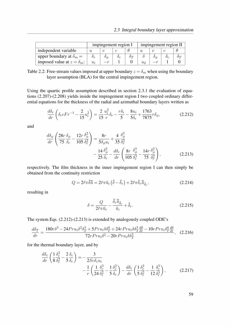
2.3 Integral boundary layer approximation
impingement region I impingement region IIindependent variable u xx v xx c xx θ xx uxx vxx c xx θxxupper boundary at δm = δr δφ δc δT δ δφ δc δTimposed value at z = δm: ui −r 1 0 uδ −r 1 0
Table 2.2: Free-stream values imposed at upper boundary z= δm when using the boundarylayer assumption (BLA) for the central impingement region.
Using the quartic profile assumption described in section 2.3.1 the evaluation of equa-tions (2.207)-(2.208) yields inside the impingement region I two coupled ordinary differ-ential equations for the thickness of the radial and azimuthal boundary layers written as
dδrdr
(δrεFr
−1− 215u2i
)=
215u2i
rδr−
rδr5− 8ui
5δr+
17637875
rδφ, (2.212)
and
dδφdr
(28r75
δφδr− 12r
105
δ2φ
δ2r
)=
8r5δφui
+4
35
δ3φ
δ2r
− 1425
δ2φ
δr− dδrdr
(8r
105
δ3φ
δ3r− 14r
75
δ2φ
δ2r
), (2.213)
respectively. The film thickness in the inner impingement region I can then simply beobtained from the continuity restriction
Q= 2rπδu= 2rπui(δ− δr
)+2rπδruδr , (2.214)
resulting in
δ =Q
2rπui−δruδrui
+ δr. (2.215)
The system Eqs. (2.212)-(2.213) is extended by analogously coupled ODE’s
dδTdr
=180rδ3−24Pruiδ2δ3
T +5Pruiδδ4T +24rPruiδδ3
Tdδdr −10rPruiδ4
Tdδdr
72rPruiδ2−20rPruiδδ3T
, (2.216)
for the thermal boundary layer, and by
dδcdr
(18δ2c
δ2r− 2
5δcδr
)=− 3
2Scδcui
− 1r
(1
24δ3c
δ2r− 1
5δ2c
δr
)− dδrdr
(15δ2c
δ2r− 1
12δ3c
δ3r
), (2.217)
59

2 Mathematical modeling and approximate solutions
for the concentration boundary layer, when including the heat transfer, and species masstransport in a binary mixture, respectively.
In the region II the boundary layer of the radial velocity component has reached the freesurface, δr = δ, and the following two ordinary differential equations for the film thicknessand the thickness of the azimuthal boundary layer are obtained:
dδ
dr
(δεFr−1− 125
864r2δ2 −10δ432
+5r2δ2
4320
)=
125864r3δ
− 56rδ2 −
3rδ5
4320
+5δ2
432r− rδ
6+
17637875
rδφ, (2.218)
and
dδφdr
(1475δφδ2 −
6105
δ2φ
δ3
)=
8r5δφ
+4
105r
δ3φ
δ3 −1475r
δ2φ
δ2
− dδdr
(6
105
δ3φ
δ4 −1475
δ2φ
δ3
). (2.219)
If heat and mass transfer are included the system (2.218)-(2.219) is extended by Eq. (2.188)and Eq. (2.201) to compute δT and δc, respectively.
Radially downstream from the position, where the boundary layer of the azimuthal velocitycomponent reaches the free surface, δφ= δ, the original formulation given by Eqs. (2.174)-(2.176) is solved assuming steady state. The system is extended by Eqs. (2.188)-(2.189),or by Eqs. (2.201)-(2.202), when heat or species mass transfer are included, respectively.
Boundary layer assumption (BLA) vs. developed film assumption (DFA)
In the following the IBL approximation, which starts the radial integration from the center,ri = 0, considering the development of the velocity boundary layers (inside region I and II,as shown in Fig. 2.4),is referred to as boundary layer assumption (BLA). On the other handthe IBL approximation, which starts the integration at a certain radial inner boundary r= riwith prescribed inlet values for δi, ui, and vi, is referred to as developed film assumption(DFA), as this approach assumes that both the velocity boundary layers δr and δφ havealready reached the free surface upstream of the inner radial boundary r = ri. The filmthickness needed by the DFA at the inner boundary, δi = δr=ri , has to be assumed, or canbe taken from CFD results, if available. The required depth-averaged inflow velocities,ui = u|r=ri , vi = v|r=ri , can be computed from the asymptotic solutions for small radii,r 1, given by Eqs. (2.186) and (2.187).
60

2.4 Modeling wet chemical surface etching
δ
r0
III
δTδrδφ
δc
δ
rr rφ ri,DFAri,BLA
Figure 2.4: Scope of boundary layer assumption (BLA) and developed film assumption(DFA).
2.4 Modeling wet chemical surface etching
In the semiconductor industry spin processors are widely used for the surface preparationof silicon wafers. One major application in this particular spin-processing technology isthe wet chemical etching. A useful parameter to determine the reaction regime of the wetchemical etching process is the Damköhler number Da. It basically relates the time scaleof the chemical reaction, τchem, to the time scale of the mass transport of the etchant intothe reactive layer, τdiff , such that
Da=τdiffτchem .
(2.220)
As the mass transport essentially relies on the diffusive transport towards the wall, thecorresponding time scale can be estimated in terms of the diffusivity of the etchant D andthe characteristic film height δ0 = (ν/Ω)1/2,
τdiff ≈δ2
0D .
(2.221)
The reactive time scale τchem is determined by the governing chemical etching mechanism,such that it scales with the inverse of the rate determining reaction rate
τchem ≈1ω .
(2.222)
61
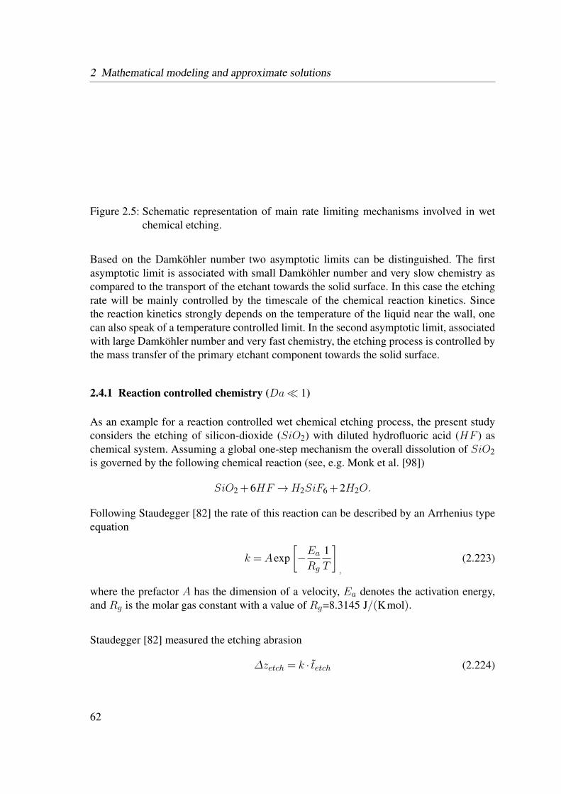
2 Mathematical modeling and approximate solutions
Figure 2.5: Schematic representation of main rate limiting mechanisms involved in wetchemical etching.
Based on the Damköhler number two asymptotic limits can be distinguished. The firstasymptotic limit is associated with small Damköhler number and very slow chemistry ascompared to the transport of the etchant towards the solid surface. In this case the etchingrate will be mainly controlled by the timescale of the chemical reaction kinetics. Sincethe reaction kinetics strongly depends on the temperature of the liquid near the wall, onecan also speak of a temperature controlled limit. In the second asymptotic limit, associatedwith large Damköhler number and very fast chemistry, the etching process is controlled bythe mass transfer of the primary etchant component towards the solid surface.
2.4.1 Reaction controlled chemistry (Da 1)
As an example for a reaction controlled wet chemical etching process, the present studyconsiders the etching of silicon-dioxide (SiO2) with diluted hydrofluoric acid (HF ) aschemical system. Assuming a global one-step mechanism the overall dissolution of SiO2is governed by the following chemical reaction (see, e.g. Monk et al. [98])
SiO2 +6HF →H2SiF6 +2H2O.
Following Staudegger [82] the rate of this reaction can be described by an Arrhenius typeequation
k = Aexp[−EaRg
1T
]
,
(2.223)
where the prefactor A has the dimension of a velocity, Ea denotes the activation energy,and Rg is the molar gas constant with a value of Rg=8.3145 J/(Kmol).
Staudegger [82] measured the etching abrasion
∆zetch = k · tetch (2.224)
62
2.4 Modeling wet chemical surface etching
for a given exposure time tetch in a number of experiments to obtain several values of kat varying temperature T . A best fit of Eq. (2.223) to these experimental data gave thevalues Ea/Rg=3978 K and A=8.29×10⁵ A/s. The so obtained reaction velocity in theconsidered range of temperature is always of the order of k=O(10−10 m/s). The diffusioncoefficient of hydrofluoric acid in an aqueous solution is of the order of D=O(10−9 m2/s)(see, e.g. Noulty et al. [99]). Assuming a typical film height of the order of δ0=O(10−4 m)as a characteristic length scale the Damköhler number for this particular surface etchingprocess can be estimated as
Da=δ0
Dk =O
(10−5
) 1, (2.225)
so that τchem τflow, and the assumption of a strongly temperature dependent, reactioncontrolled chemistry with abundance of the main reactive agent is justified.
2.4.2 Diffusion controlled chemistry (Da 1)
The present study considers the etching of silicon (Si) with an aqueous etchant consistingbasically of nitric acid (HNO3) and hydrofluoric acid (HF ) as an example for a diffusioncontrolled wet chemical etching process. Schwartz and Robbins [100] proposed a simpli-fied two-step fast reaction mechanism for the dissolution of Si as
Si+4HNO3→ SiO2 +4NO2 +2H2O
SiO2 +6HF →H2SiF6 +2H2O.
Following Kaneko et al. [68], for low HNO3 and high HF concentrations, the rate ofthis reaction is essentially controlled by the first reaction step. Since this key reaction isassumed as very fast, the Damköhler number is very high, Da 1. This implies thatthe etching reaction is limited by the diffusive flux of the nitric acid molecules towardsthe surface of the wafer. The diffusion coefficient of nitric acid in an aqueous solutionis D=2.4×10⁻⁹ m2/s, and the typical film height is of the order of δ0=O(10−4 m). Thevelocity of diffusion is thus approximately in the order of D/δ0 ≈O(10−5 m/s).The etching abrasion rate R is proportional to the mass flux of dissolved silicon jSi, i.e.
R ∝jSiρSi
[m/s]. (2.226)
Assuming a stoichiometric oxidation of silicon by nitric acid,
jSiMSi
=−14jHNO3
MHNO3
, (2.227)
63
2 Mathematical modeling and approximate solutions
Eq. (2.226) can be rewritten as
R ∝−jHNO3
14ρSi
MSi
MHNO3
[m/s]. (2.228)
The diffusive mass flux of the primary etchant species is given by
jHNO3 =−ρD∂c
∂z
∣∣∣∣z=0
[kg/(m2s)], (2.229)
which can be rewritten as in terms of the local Sherwood number
Sh=∂c
∂z
∣∣∣∣z=0
, (2.230)
asjHNO3 =−ρD
ciδ0Sh. (2.231)
The etching rate for a diffusion controlled chemistry is proportional to the Sherwood num-ber and computed from
R= k1ρSi
MSi
4MHNO3
ρDciδ0Sh [m/s] (2.232)
using the values ρSi=2329 kg/m3, MSi=28.09 g/mol, MHNO3=63.01 g/mol, and an em-pirical proportionality constant k.
64
3 NUMERICAL SOLUTIONS
3.1 Numerical solution of the Navier-Stokes equations
In the CFD based approach, the unsteady, axisymmetric Navier-Stokes equations (2.37)-(2.38), as well as the energy equation (2.39), or, alternatively, the convection-diffusionequation for a species in a binary mixture, Eq. (2.40), are discretized and numericallysolved using the flow simulation software ANSYS FLUENT [101, 102]. In this generalpurpose CFD code a cell-centered finite-volume method is employed.
3.1.1 Finite Volume Method
The general transport equation for an arbitrary tensorial flow quantity ϕ(~x,t) is given by
∂ρϕ
∂t︸︷︷︸(i)
+∇ · (ρ~vϕ)︸ ︷︷ ︸(ii)
= ∇ · (Γ∇ϕ)︸ ︷︷ ︸(iii)
+Sϕ(ϕ)︸ ︷︷ ︸(iv)
. (3.1)
Here Γ denotes the diffusivity and Sϕ(ϕ) represents a source term. The individual termsin Eq. (3.1) represent the change per unit volume (i), the flux due to convection (ii), thetransport due to diffusion (iii), and the rate of production (iv), respectively.
A finite volume discretization of Eq. (3.1) is obtained by integrating over a finite controlvolume VP and time ∆t,
t+∆t∫
t
∫
VP
∂ρϕ
∂tdV +
∫
VP
∇ · (ρ~vϕ)dV
dt=
t+∆t∫
t
∫
VP
(∇ · (Γ∇ϕ)+Sϕ(ϕ))dV
dt. (3.2)
The volume integral with the transient term can be approximated first-order accurate intime as
∫
V
∂ρϕ
∂tdV ≈ ρn+1
P ϕn+1P −ρnPϕnP∆t
VP , (3.3)
65
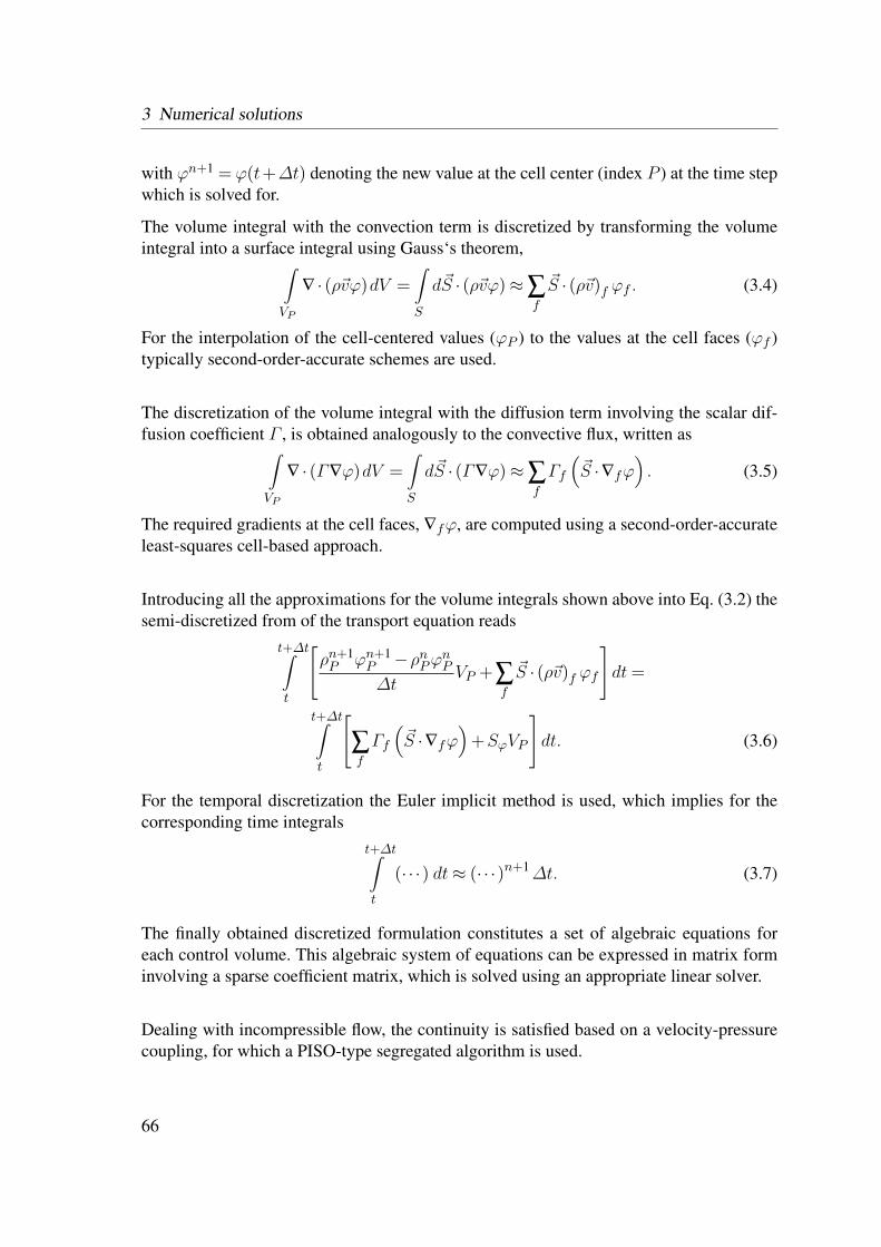
3 Numerical solutions
with ϕn+1 = ϕ(t+∆t) denoting the new value at the cell center (index P ) at the time stepwhich is solved for.
The volume integral with the convection term is discretized by transforming the volumeintegral into a surface integral using Gauss‘s theorem,
∫
VP
∇ · (ρ~vϕ)dV =∫
S
d~S · (ρ~vϕ)≈∑f
~S · (ρ~v)f ϕf . (3.4)
For the interpolation of the cell-centered values (ϕP ) to the values at the cell faces (ϕf )typically second-order-accurate schemes are used.
The discretization of the volume integral with the diffusion term involving the scalar dif-fusion coefficient Γ , is obtained analogously to the convective flux, written as
∫
VP
∇ · (Γ∇ϕ)dV =∫
S
d~S · (Γ∇ϕ)≈∑f
Γf
(~S ·∇fϕ
). (3.5)
The required gradients at the cell faces, ∇fϕ, are computed using a second-order-accurateleast-squares cell-based approach.
Introducing all the approximations for the volume integrals shown above into Eq. (3.2) thesemi-discretized from of the transport equation reads
t+∆t∫
t
[ρn+1P ϕn+1
P −ρnPϕnP∆t
VP +∑f
~S · (ρ~v)f ϕf]dt=
t+∆t∫
t
[∑f
Γf
(~S ·∇fϕ
)+SϕVP
]dt. (3.6)
For the temporal discretization the Euler implicit method is used, which implies for thecorresponding time integrals
t+∆t∫
t
(· · ·) dt≈ (· · ·)n+1∆t. (3.7)
The finally obtained discretized formulation constitutes a set of algebraic equations foreach control volume. This algebraic system of equations can be expressed in matrix forminvolving a sparse coefficient matrix, which is solved using an appropriate linear solver.
Dealing with incompressible flow, the continuity is satisfied based on a velocity-pressurecoupling, for which a PISO-type segregated algorithm is used.
66

3.1 Numerical solution of the Navier-Stokes equations
3.1.2 Volume of Fluid Method
The description of the two-phase flow is accomplished using the implemented Volume-of-Fluid method (Hirt and Nichols [103]). In this one-fluid formulation, both phases aretreated as single continuum, distinguished by a phase-marker function, which is definedas
γ(~x,t) =
1 liquid phase,0 gas phase,0 < γt < 1 transitional zone.
(3.8)
The interface between the phases is tracked solving the phase-marker transport equation
∂γ
∂t+~v ·∇γ = 0. (3.9)
The transitional zone basically represents the interface, where the fluid properties like den-sity or viscosity exhibit a discontinuous step in reality. This transitional zone is here con-sidered to have a small finite thickness t, which is necessary to model the two fluids asa continuum, using the continuity and the momentum equations. The fluid properties, forexample the density of the fluid, are determined using the volume-weighted average
ρ= γρL+(1−γ)ρG. (3.10)
Here the indices L andG denote the properties of the liquid and the gas phase, respectively.
To guarantee the boundedness of the phase-marker function γ, and to prevent an unphys-ical smearing of the step-like change at the phase interface an adequate discretization ofthe phase-marker transport equation has to be employed. For this purpose, the simulationpackage offers different numerical methods for correcting the fluxes across the faces ofthe control volumes, from which the High Resolution Interface Capturing scheme (HRIC,Muzaferija et al. [104]) was chosen. This HRIC scheme represents a hybrid scheme basedon the blending of bounded downwind and upwind differencing schemes.
In the framework of the implemented VoF method the effect of surface tension is modeledbased on the continuum surface force (CSF) model, which was proposed by Brackbill etal. [105]. In this model the capillary force is incorporated in the momentum equationsin terms of an appropriate volume force, which is proportional to the curvature of theinterface.
67
3 Numerical solutions
3.1.3 Setup
The computational domain and the boundary conditions used in the CFD simulations aresketched in Fig. 3.1. At the liquid inflow boundary a uniform inlet velocity boundary con-dition, equivalent to the considered volumetric flowrate, was prescribed. The inflow tem-perature, or alternatively the inflow species mass fraction, were assumed to be constant.The radially inner boundary represents an axis of symmetry, so that symmetry boundaryconditions, which are basically zero-gradient conditions, apply. At the upper and radiallyouter boundaries, pressure outlet boundary conditions were imposed. This boundary con-dition implies, that the static pressure is prescribed relative to the operating pressure, whileall other flow quantities are extrapolated from the interior.
At the surface of the rotating disk a solid wall boundary condition is used, which is as-sociated with no-slip conditions setting the velocity of the liquid equal to the rotationalspeed of the disk. Furthermore a constant heat flux was assumed for the thermal boundarycondition at the wall, while a constant species mass fraction was assumed when modelingthe mass transport in a binary mixture.
The steady-state smooth film solutions of the IBL model, presented in Sec. 2.3.4, wereused to initialize the volume fraction distribution and the flow field inside the film.The properties of the three different fluids considered as the liquid phase in the CFD sim-ulations are listed in Tab. 3.1. For the ambient gas phase the properties of air were used,with ρG = ρa =1.225 kg/m3, νG = νa =1.46×10⁻⁵ m2/s.
ΩR
wall boundary
free surface
outer boundaries
inflow boundary
symmetry axis
~
r~
z
Figure 3.1: Computational domain and boundary conditions.
68

3.2 Numerical solution of the integral boundary layer equations
ρ [kg/m3] ν [m2/s] σ [N/m]L1 998.2 1.0×10⁻⁶ 0.072L2 990 1.3×10⁻⁶ 0.072L3 998.2 2.87×10⁻⁶ 0.072
Table 3.1: Properties of liquids considered in the CFD simulations.
The computational domain shown in Fig. 3.1 was discretized using approximately 124thousand cells. The rectangular-shaped cells were layered in five rows. The first layer ex-tended from the surface of the disk to z=0.005 mm and consisted of 10 rows of equallysized cells. In the second layer, which extended to z=0.1 mm, 40 rows of equally sized cellswere stacked upon each other. From the third layer onwards the vertical height of the cellswas successively increased. The radial region was subdivided in three evenly spaced cellcolumns, with a radial cell size of ∆r=0.1 mm. In the region covered by liquid additionalrefinement was performed using a twice as fine resolution in both directions.
The time step size for the simulation was allowed to vary depending on the flow conditionsusing the Courant-Friedrichs-Lewy (CFL) criterion. The time step size typically variedbetween 1÷5×10⁻⁵ s.
3.2 Numerical solution of the integral boundary layer equations
The IBL approximation leads to a nonlinear system of hyperbolic partial differential equa-tions (PDEs), defined by Eqs. (2.132), extended by Eqs. (2.154) to model the heat transfer,and by Eq. (2.162) to model the species mass transfer.
In the following the single spacial dimension is denoted by x and the vector of the de-pendent state variables by ~U(x,t) ∈Rm. Considering furthermore the m-dimensional fluxfunction to be denoted with ~F (~U(x,t)) ∈Rm, and the vector of source terms to be writtenas ~S(~U(x,t),x, t) ∈ Rm, the nonlinear system of hyperbolic partial differential equationscan be written in general form as
∂~U(x,t)
∂t+∂ ~F (~U(x,t))
∂x= ~S(~U(x,t),x, t). (3.11)
Such time-dependent systems of PDEs are frequently encountered when modeling convec-tion dominated transport processes. For the special case of a system of conservation laws,which is associated with ~S ≡ 0, a change in the state variables can only be due to a netflux.
69

3 Numerical solutions
3.2.1 Hyperbolic systems
The system defined in Eq. (3.11) is called hyperbolic, if the m×m Jacobian matrix
J(~U) =∂ ~F (~U)
∂~U(3.12)
• has real eigenvalues λp(~U) and a corresponding complete set of m linearly indepen-dent eigenvectors ~rp(~U), (p= 1, ...,m), and
• is diagonalizable: J =RΛR−1.
Therein, Λ is a diagonal matrix holding the real eigenvalues λp andR is the invertible righteigenvector matrix, with the corresponding eigenvectors ~rp as its columns.Numerical methods for solving such time-dependent hyperbolic systems are based on solv-ing Riemann problems. For this reason the concepts of solving Riemann problems arerecalled (see, e.g. Toro [106], LeVeque [107, 108]), before proceeding to the numericalapproach.
Riemann problem for a linear hyperbolic system
The initial value problem (IVP) for a linear hyperbolic system
∂~U(x,t)
∂t+A
∂~U(x,t)
∂x= 0, (3.13)
with constant coefficient matrix A, defined together with an initial condition of the form
~U(x,0) = ~U0(x) , −∞ < x < ∞ (3.14)
can be explicitly solved. For this purpose a transformation into so called characteristicvariables, defined by
~W =R−1~U, (3.15)
is performed. The flux function is in this case simply given as
~F (~U(x,t)) = A~U(x,t). (3.16)
Multiplication of Eq. (3.13) from left with R−1 results in
R−1∂~U(x,t)
∂t+ΛR−1∂
~U(x,t)
∂x= 0. (3.17)
70
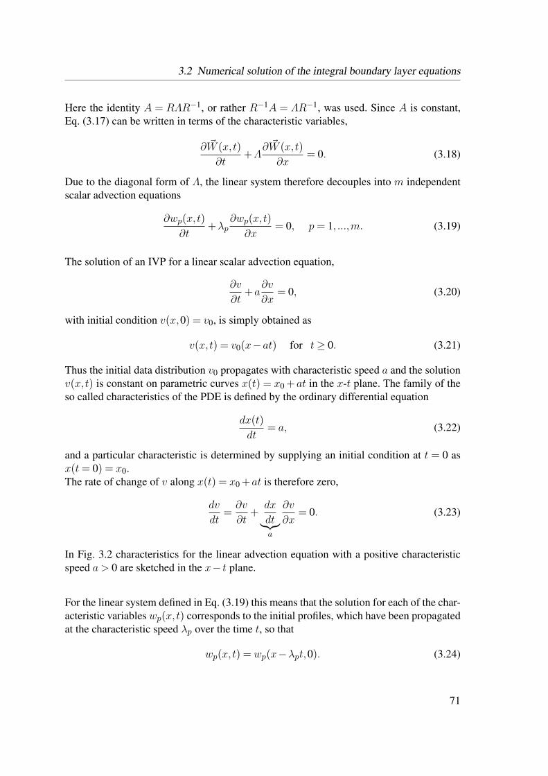
3.2 Numerical solution of the integral boundary layer equations
Here the identity A = RΛR−1, or rather R−1A = ΛR−1, was used. Since A is constant,Eq. (3.17) can be written in terms of the characteristic variables,
∂ ~W (x,t)
∂t+Λ
∂ ~W (x,t)
∂x= 0. (3.18)
Due to the diagonal form of Λ, the linear system therefore decouples into m independentscalar advection equations
∂wp(x,t)
∂t+λp
∂wp(x,t)
∂x= 0, p= 1, ...,m. (3.19)
The solution of an IVP for a linear scalar advection equation,
∂v
∂t+a
∂v
∂x= 0, (3.20)
with initial condition v(x,0) = v0, is simply obtained as
v(x,t) = v0(x−at) for t≥ 0. (3.21)
Thus the initial data distribution v0 propagates with characteristic speed a and the solutionv(x,t) is constant on parametric curves x(t) = x0 +at in the x-t plane. The family of theso called characteristics of the PDE is defined by the ordinary differential equation
dx(t)
dt= a, (3.22)
and a particular characteristic is determined by supplying an initial condition at t = 0 asx(t= 0) = x0.The rate of change of v along x(t) = x0 +at is therefore zero,
dv
dt=∂v
∂t+
dx
dt︸︷︷︸a
∂v
∂x= 0. (3.23)
In Fig. 3.2 characteristics for the linear advection equation with a positive characteristicspeed a > 0 are sketched in the x− t plane.
For the linear system defined in Eq. (3.19) this means that the solution for each of the char-acteristic variables wp(x,t) corresponds to the initial profiles, which have been propagatedat the characteristic speed λp over the time t, so that
wp(x,t) = wp(x−λpt,0). (3.24)
71

3 Numerical solutions
The solution of the original system, defined in Eq. (3.13), is finally obtained by the inversetransformation,
~U(x,t) =R ~W (x,t). (3.25)
This procedure can be written in terms of an eigenvector expansion of ~U(x,t) with coeffi-cients wp(x,t) as
~U(x,t) =m
∑p=1
wp(x,t)~rp, (3.26)
or, when using Eq. (3.24), as
~U(x,t) =m
∑p=1
wp(x−λpt,0)~rp. (3.27)
Thus, the solution can be interpreted as superposition of m waves with constant shapewp(x,0)~rp, which propagate independently with speed λp.Denoting the rows of matrix R−1 by (~lp)
T , the p-th component of R−1~U can be written as(cf. (3.15))
wp(x,t) =(~lp
)T· ~U(x,t). (3.28)
Substituting this expression into the coefficients of the eigenvector expansion Eq. (3.27)can be rewritten as
~U(x,t) =m
∑p=1
[(~lp)
T · ~U(x−λpt,0)]~rp. (3.29)
A Riemann problem is generally defined by a hyperbolic PDE system together with a
0x
x=x0+at
t
x
0
Figure 3.2: Sketch of the characteristics of the linear advection equation for a characteristicspeed a > 0 in the x− t plane.
72
3.2 Numerical solution of the integral boundary layer equations
piecewise constant initial condition of the form
~U(x,0) =
~UL x < 0~UR x > 0.
(3.30)
For the simple case of a linear hyperbolic system with a constant coefficient matrix A(Eq. (3.13)) the general solution is provided by Eq. (3.29). Assuming additionally, that thereal eigenvalues of A are distinct and ordered,
λ1 < λ2 < ... < λm, (3.31)
the initial condition can be written as eigenvector expansion with constant coefficients αand β as
~UL =m
∑p=1
αp~rp and ~UR =m
∑p=1
βp~rp. (3.32)
As sketched in Fig. 3.3 the general solution of this linear Riemann problem can then beinterpreted as a superposition ofmwaves, which originate from the point (0,0) in the x− tplane.
Each of these waves carries a discontinuity in each component of ~U and travels at constantspeed λp. In terms of the characteristic variables, the initial condition is provided by
wp(x,0) =
αp, x < 0βp, x > 0
(3.33)
and the solution to the scalar Riemann problems is obtained as
wp(x,t) = wp(x−λpt,0) =αp, x−λpt < 0βp, x−λpt > 0.
(3.34)
0
t
x
UUL R
λ
λλ
λ
λ1
23
4
5
Figure 3.3: Sketch of the solution structure of a linear Riemann problem withm= 5 waves.
73

3 Numerical solutions
0
λ3
α r11
dx/dt= λ1
x
β1r1+β
2r2
+β3r3
λ2
β1r1β2
r2
++ α3 3
r
22 33α rα r+ +
11+ 2α 2r +α
3 3rrβ
Figure 3.4: Sketch of the values of the solution in different sectors of a Riemann problemwith m= 3 waves.
The solution to the original system can finally be written as
~U(x,t) =P (x,t)
∑p=1
βp~rp+m
∑P (x,t)+1
αp~rp. (3.35)
Therein, the integer P (x,t) denotes the maximum value of p ∈ [1, ...,m], for which theinequality,
x−λpt > 0, (3.36)
holds.
Fig. 3.4 provides an illustration for the determination of ~U(x,t) in case of a linear Rie-mann problem with m= 3 waves. For any point in between two characteristics, defined bydx/dt = const., the solution is the same. To the left of the λ1-characteristic the solutionis simply the initial data ~UL. Similarly, to the right of the λ3-characteristic, the solutionis given by the initial data ~UR. The coefficients of the eigenvector expansion for the so-lutions in between the waves are determined from Eq. (3.34). As soon as one crosses thep-th characteristic, dx/dt = λp, the value of x− λpt changes from negative to positive,corresponding to a change of the coefficient from αp to βp.
3.2.2 Numerical solution of hyperbolic PDE systems
Finite volume methods, which are based on the integral form of the transport equations,are especially suited for the numerical solution of hyperbolic PDE systems. The integral
74
3.2 Numerical solution of the integral boundary layer equations
form for a system of conservation laws reads
d
dt
x2∫
x1
~U(x,t)dx= ~F (~U(x1, t))− ~F (~U(x2, t)) ∀x1,x2. (3.37)
Discretizing the x-t plane utilizing a mesh of width h=∆x, and a time step size k =∆t,the discrete points (xj , tn) are given as
xj = jh, j = ...,−1,0,1,2, ...tn = nk, n= 0,1,2, ... .
(3.38)
The coordinates of the left and right faces of the j-th cell are denoted by xj−1/2 = xj−h/2and xj+1/2 = xj +h/2, respectively. The pointwise value of an approximation to the cellaverage of ~U(x,t) is then defined as
Unj =1∆x
xj+1/2∫
xj−1/2
~U(x,tn)dx. (3.39)
Integration of Eq. (3.37) with respect to time, between tn and tn+1, and division by ∆xfinally provides the discretized time integration scheme for the numerical approximationof the cell average of the j-th cell
Un+1j = Unj −
∆t
∆x
[Fnj+1/2−Fnj−1/2
]. (3.40)
Here Fnj±1/2 is the numerical approximation of the flux vector ~F (~U) at the left and rightcell faces,
Fnj±1/2 ≈1∆t
tn+1∫
tn
~F (~U(xj±1/2, t))dt. (3.41)
As sketched in Fig. 3.5, the finite volume based discretization leads to a piecewise-constantdistribution of the cell averaged state variables, constituting a sequence of local Riemannproblems at the cell interfaces. Thus, the task of the numerical solution of the hyperbolicPDE system is to solve these local Riemann problems to update the solution to the newtime level Un+1
j .
Using Godunov’s method, which was developed in 1959 for gas dynamics, the indepen-dent Riemann problems are solved exactly over a short time interval. Since for nonlinearproblems the solution of the sequence of Riemann problems at each time step is computa-tionally expensive, the approximate Riemann solver is used as a more efficient approach.This approximation approach is also justified by the fact that even the Godunov scheme isonly first-order accurate in space and time, due to the piecewise constant representation ofthe state variables.
75

3 Numerical solutions
x
nUj
j−2 j−1 j j+1 j+2
Figure 3.5: Piecewise constant distribution of a cell averaged state variable.
Roe’s approximate Riemann solver
One of the most popular approximate Riemann solvers goes back to Roe [109] and isbased on a linearization of the nonlinear problem. In this approach the nonlinear hyperbolicsystem
∂~U(x,t)
∂t+~F (~U(x,t))
∂x= 0, (3.42)
with initial conditions
~U(x,0) =
~UL x < 0~UR x > 0,
(3.43)
which results in a sequence of nonlinear Riemann problems at the individual cell interfaces,is replaced by a linear approximation
∂~U(x,t)
∂t+ A
∂ ~U(x,t)
∂x= 0, (3.44)
with a constant coefficient matrix A. This Roe matrix A is assumed to be constant betweentwo cells and is assumed to be a function of the corresponding states to the left and right ofthese cells, which are denoted by the subscripts L and R, respectively. As such the approx-imation is essentially based on a linearization together with the assumption of constantaverage states at the cell interfaces.
The constant coefficient Roe matrix A must guarantee the
• hyperbolicity of the system, that is A has to be diagonalizable with real eigenvalues,
76
3.2 Numerical solution of the integral boundary layer equations
• conservation across discontinuities, that is
~F (~UR)− ~F (~UL) = A(~UR− ~UL), (3.45)
• consistency with the exact Jacobian, that is
~UL, ~UR→ ~U : A→ ∂ ~F (~U)
∂~U. (3.46)
A suitable approximate Jacobian A for the numerical solution of the IBL equations can beobtained using the arithmetic average for the film thickness
δ =12(δL+ δR) , (3.47)
and Roe averages for the remaining state variables, which is for example for the depth-averaged radial velocity u given by
u=
√δLuL+
√δRuR√
δL+√δR
. (3.48)
The obtained sequence of linearized Riemann problems is then solved exactly. For thispurpose, considering exemplarily the Riemann problem at the face xj−1/2, the left andright states at the cell interface, UnL = Unj−1 and UnR = Unj , respectively, are decomposedinto a linear combination of right eigenvectors of A
Unj−1 =m
∑p=1
αpj−1rp,
Unj =m
∑p=1
βpj rp.
(3.49)
Here and below the summation index p is displayed as superscript, while the superscriptdenoting the current time level n is dropped in the sums on the RHS for reasons of read-ability.The change in the state variables across the face between the neighboring cells is decom-posed into a superposition of m wavesW ,
(∆U)nj−1/2 = Unj −Unj−1 =m
∑p=1
(βpj −α
pj−1
)rp =
=m
∑p=1
γpj−1/2r
p =m
∑p=1Wpj−1/2.
(3.50)
77

3 Numerical solutions
The coefficients of the eigenvector expansion are determined according to Eq. (3.28), sothat the p-th wave in the Riemann solution at time level n is obtained as
Wpj−1/2 =
(lpj−1/2
)T(Uj−Uj−1) r
pj−1/2. (3.51)
These jumps propagate with velocities λp, respectively, the eigenvalues of the system. Thefluxes required for updating the averaged cell value in the j-th cell (cf. Eq. (3.40)) aredetermined from several right going waves with positive velocity (λp)+, starting from thej− 1/2 cell interface, and several left going waves with negative velocity (λp)−, startingfrom the j+1/2 cell interface, respectively. The expression for updating the cell averagereads
Un+1j = Unj −
∆t
∆x
[m
∑p=1
(λp)+Wp
j−1/2−m
∑p=1
(λp)−Wp
j+1/2
]. (3.52)
Introducing the notation
A− = R diag((λp)
−)R−1, λ− =min(λ,0),
A+ = R diag((λp)
+)R−1, λ+ =max(λ,0),
(3.53)
this scheme can also be written as
Un+1j = Unj −
∆t
∆x
[A+∆Uj−1/2 + A
−∆Uj+1/2]. (3.54)
Higher order correction terms and flux limiter
An extension to a high resolution method is achieved by adding an additional term, whichprovides limited second-order correction fluxes,
Un+1j = Unj −
∆t
∆x
[A+∆Uj−1/2 + A
−∆Uj+1/2]− ∆t
∆x
[Fj+1/2− Fj−1/2
]. (3.55)
The correction fluxes are given by
Fj±1/2 =12
m
∑p=1
(1− ∆t
∆x
∣∣∣λpj±1/2
∣∣∣)∣∣∣λpj±1/2
∣∣∣Wpj±1/2. (3.56)
Here Wpj±1/2 represents a limited version of the wave, which is obtained by multiplication
with a limiter function χ(µpj±1/2
), which measures the smoothness of the solution, as
Wpj±1/2 = χ
(µpj±1/2
)Wpj±1/2. (3.57)
78

3.2 Numerical solution of the integral boundary layer equations
The parameter µ of the limiter function, is defined as
µpj−1/2 =
WpJ−1/2W
pj−1/2∣∣∣Wp
j−1/2
∣∣∣, (3.58)
with
J =
j−1 if λp > 0j+2 if λp < 0.
(3.59)
For smoothly varying data the limiter function approaches unity and the additional term inEq. (3.55) provides a useful correction, improving the accuracy of the numerical solution.Near discontinuities the limiter modifies the wave, typically by reducing its magnitude. Apopular high-resolution limiter is the superbee limiter
χ(µ) = max [0,min(1,2µ) ,min(2,µ)] , (3.60)
which was used in the present work. Linear alternative approaches are for example theupwind method (χ(µ) = 0) and the unstable Lax-Wendroff scheme with χ(µ) = 1.
Source term treatment
To properly account for the presence of source terms in the numerical solution of a hyper-bolic PDE system, a popular approach is to split the problem of solving
∂~U(x,t)
∂t+∂ ~F (~U(x,t))
∂x= ~S(~U(x,t),x, t). (3.61)
into two sub-problems
∂~U(x,t)
∂t+∂ ~F (~U(x,t))
∂x= 0, (3.62)
∂~U(x,t)
∂t= ~S(~U(x,t),x, t). (3.63)
The main advantage using this operator splitting approach is that for each subprobleman appropriate scheme can be chosen. Therefore, this fractional step scheme was used inthe present work for the numerical solution of the governing IBL equations. In particular,Roe’s approximate Riemann solver with flux-limited second-order correction terms wasapplied to the sub-problem associated with the homogeneous conservation laws, definedby Eq (3.62), while a two-stage Runge-Kutta scheme was chosen for the integration of theODEs defined by Eq. (3.63).
79

3 Numerical solutions
3.2.3 Setup
For the practical implementation of the hyperbolic solver numerical routines from theFortran-library CLAWPACK (Conservation Laws Package) [110] were used. This Fortran-library provides the wave-propagation algorithm of Eq. (3.55), which requires
• the fluctuations A±∆Uj−1/2,
• the wavesWpj−1/2, and
• the local speeds λpj−1/2,
for the considered system of IBL equations. To provide these input data a proper routinewas programmed and implemented along with a source term routine for the fractional-stepmethod.
ri
δT
δφ
δr
δ
δ
r0 1 2 3 4
0
0.5
1
1.5
2
(a)
ri
δc
δφ
δr
δ
δ
r0 1 2 3 4
0
0.5
1
1.5
2
(b)
Figure 3.6: Initial conditions for the film thickness and position of the inflow boundaryri for the numerical solution of the unsteady IBL equations (a) including heattransfer, (b) including species mass transfer.
Initialization and boundary conditions
Generally the unsteady flow simulation is initialized from the corresponding steady-statesolutions of the IBL model using the boundary layer assumption, as discussed in Sec. 2.3.4,computed for the whole disk.The inflow conditions are set at a certain radial inner position ri, where a smooth filmsolution can be expected, so that appropriate inlet conditions can be obtained from the
80

3.2 Numerical solution of the integral boundary layer equations
corresponding steady-state solutions. In the case of heat transfer the unsteady simulationstarts from the radial position ri = rT , where the film is hydrodynamically and thermallyfully developed, as shown in Fig. 3.6(a). On the other hand, in the case of species masstransfer, the unsteady IBL simulation starts from an inner radius where the flow is hydro-dynamically fully developed, associated with ri = r|δφ=δ, as shown in Fig. 3.6(b). Thisdifferent setting of the radial inner boundary is due to the very high Schmidt numbers,which are considered in the present case. For the here relevant Schmidt number of the or-der of O
(10−3) the concentration boundary layers are very thin, so that they may never
reach the film surface throughout the domain as exemplarily shown in Fig. 3.6(b).At the radially outer boundary the flow quantities are linearly extrapolated from the inte-rior.
81


4 RESULTS AND DISCUSSION
The following discussion of the computational results starts with a comprehensive analysisof the steady-state solutions. It is followed by the analysis of the unsteady solutions, whichshall particularly highlight the effect of the unsteady surface waves on the hydrodynamics,the heat and species mass transfer. The whole discussion is based on three cases listed withtheir determining parameters in Tab. 4.1.
The considered cases were specially selected to cover smooth film as well as wavy filmconditions, and providing also experimental data for validation.
Case Q [lpm] n [rpm] ν [m2/s] εFr−1 W Pr Sc
C1 1.8 401 1.3×10⁻⁶ 5×10⁻⁴ 1.9×10⁻⁷
C2 1 500 1×10⁻⁶ 4.5×10⁻⁴ 3×10⁻⁶ 7C3 1.25 500 2.87×10⁻⁶ 1.03×10⁻³ 9.35×10⁻⁶ 1196
Table 4.1: Considered test cases for steady-state smooth film and for wavy flow conditions.
The discussion of the hydrodynamic characteristics is mainly based on the case C1. Forthis particular case experimental data for the film thickness are available from Burns etal. [65]. The case C2 is focused on the investigation of the thermal characteristics of thefilm flow, while the case C3 is focused on the description of the species mass transfer in abinary mixture on the spinning disk. Assuming the asymptotic regimes of very small andvery large Damköhler numbers for the process of wet chemical etching, the predictions forthe temperature considered in case C2, and the species mass transport considered in caseC3, translate directly into predictions for the etching rates, for which experimental resultsare available from Staudegger et al. [82, 85]. The validation of the present unsteady IBLmodel against the experimental data is comprehensively discussed in Sec. 4.3.
4.1 Steady-state solutions
In this section the steady-state results of the IBL equations for smooth, axisymmetric floware discussed and compared against results from the analytical far-field solutions. Theanalysis of the predictions obtained for the heat transfer also includes a comparison againstCFD results.
83
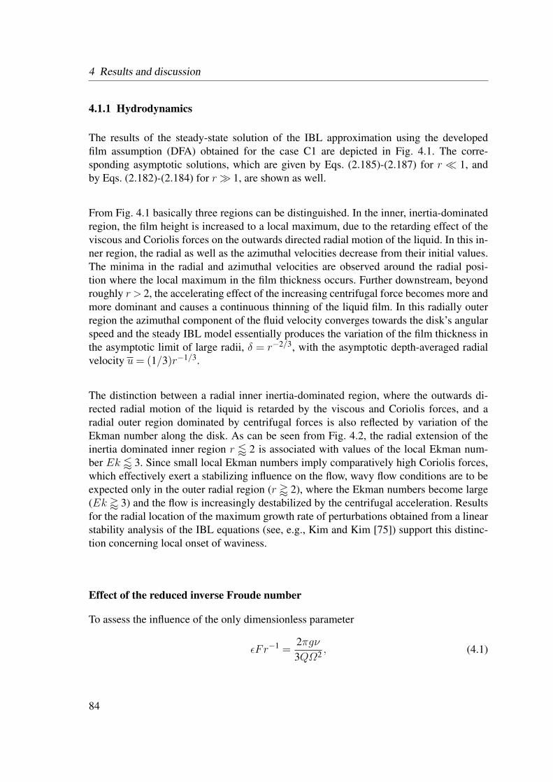
4 Results and discussion
4.1.1 Hydrodynamics
The results of the steady-state solution of the IBL approximation using the developedfilm assumption (DFA) obtained for the case C1 are depicted in Fig. 4.1. The corre-sponding asymptotic solutions, which are given by Eqs. (2.185)-(2.187) for r 1, andby Eqs. (2.182)-(2.184) for r 1, are shown as well.
From Fig. 4.1 basically three regions can be distinguished. In the inner, inertia-dominatedregion, the film height is increased to a local maximum, due to the retarding effect of theviscous and Coriolis forces on the outwards directed radial motion of the liquid. In this in-ner region, the radial as well as the azimuthal velocities decrease from their initial values.The minima in the radial and azimuthal velocities are observed around the radial posi-tion where the local maximum in the film thickness occurs. Further downstream, beyondroughly r > 2, the accelerating effect of the increasing centrifugal force becomes more andmore dominant and causes a continuous thinning of the liquid film. In this radially outerregion the azimuthal component of the fluid velocity converges towards the disk’s angularspeed and the steady IBL model essentially produces the variation of the film thickness inthe asymptotic limit of large radii, δ = r−2/3, with the asymptotic depth-averaged radialvelocity u= (1/3)r−1/3.
The distinction between a radial inner inertia-dominated region, where the outwards di-rected radial motion of the liquid is retarded by the viscous and Coriolis forces, and aradial outer region dominated by centrifugal forces is also reflected by variation of theEkman number along the disk. As can be seen from Fig. 4.2, the radial extension of theinertia dominated inner region r / 2 is associated with values of the local Ekman num-ber Ek / 3. Since small local Ekman numbers imply comparatively high Coriolis forces,which effectively exert a stabilizing influence on the flow, wavy flow conditions are to beexpected only in the outer radial region (r ' 2), where the Ekman numbers become large(Ek ' 3) and the flow is increasingly destabilized by the centrifugal acceleration. Resultsfor the radial location of the maximum growth rate of perturbations obtained from a linearstability analysis of the IBL equations (see, e.g., Kim and Kim [75]) support this distinc-tion concerning local onset of waviness.
Effect of the reduced inverse Froude number
To assess the influence of the only dimensionless parameter
εFr−1 =2πgν3QΩ2 , (4.1)
84

4.1 Steady-state solutions
asympt. r ≫ 1
asympt. r ≪ 1
IBL quart.δ
r
0 1 2 3 4 50
0.5
1
1.5
2
(a) Film thickness vs. radial distance.
asympt. r ≫ 1
asympt. r ≪ 1
IBL quart.
u
r
0 1 2 3 4 50
0.2
0.4
0.6
0.8
(b) Depth-averaged radial velocity vs. radial distance.
asympt. r ≫ 1
asympt. r ≪ 1
IBL quart.
v
r
0 1 2 3 4 5−0.5
−0.4
−0.3
−0.2
−0.1
0
(c) Depth-averaged azimuthal velocity vs. radial distance.
Figure 4.1: Solutions of the steady-state IBL equations for the case C1 together with theasymptotic solutions in the radially inner and outer regions.
85

4 Results and discussion
Ek
r
0 1 2 3 4 50
1
2
3
4
5
6
7
8
9
Figure 4.2: Ekman number Ek = ν/Ωδ2 vs. radial distance for the case C1.
which appears in the governing set of equations for the steady-state smooth film flow,Eqs. (2.174)-(2.176), a parametric study was carried out varying the values of the reducedinverse Froude number between 8× 10⁻⁵ - 6× 10⁻². This range of the reduced inverseFroude number covers most available experimental data, and is also practically relevant forthe semiconductor industry, where spinning disk devices are used for the surface prepara-tion of silicon wafers.
Fig. 4.3(a) depicts the results from the steady-state IBL model, assuming a quartic ra-dial velocity profile (IBL quart.), obtained for a sub-range with the lower values εFr−1 ∈[8×10−5,9.3×10−4]. The predictions for the film thickness remain very close to each
other, indicating no significant effect of the reduced inverse Froude number in this sub-range. In Fig. 4.3(b) the results for the sub-range with the larger values of the reducedinverse Froude number, εFr−1 ≥ 10−3, are shown. The local maximum in the film heightis evidently shifted to smaller radii with increasing values of εFr−1. Furthermore, the filmthickness is found to decrease in the region of the local minimum as εFr−1 becomes larger.
The denominator in Eq. (2.180) vanishes for a critical value
(εFr−1)
crit=
ka9β1r2δ2 , (4.2)
which makes the formulation singular. Due to this singularity a radially continuous integra-tion is not possible anymore, as can for example be seen in Fig. 4.3(b) from the unphysical
86
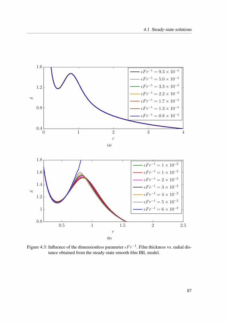
4.1 Steady-state solutions
ǫFr−1 = 0.8× 10⁻⁴
ǫFr−1 = 1.3× 10⁻⁴
ǫFr−1 = 1.7× 10⁻⁴
ǫFr−1 = 2.2× 10⁻⁴
ǫFr−1 = 3.3× 10⁻⁴
ǫFr−1 = 5.0× 10⁻⁴
ǫFr−1 = 9.3× 10⁻⁴
δ
r
0 1 2 3 40.4
0.8
1.2
1.6
(a)
ǫFr−1 = 6× 10⁻²
ǫFr−1 = 5× 10⁻²
ǫFr−1 = 4× 10⁻²
ǫFr−1 = 3× 10⁻²
ǫFr−1 = 2× 10⁻²
ǫFr−1 = 1× 10⁻²
ǫFr−1 = 1× 10⁻³
δ
r
0.5 1 1.5 2 2.50.8
1
1.2
1.4
1.6
1.8
(b)
Figure 4.3: Influence of the dimensionless parameter εFr−1. Film thickness vs. radial dis-tance obtained from the steady-state smooth film IBL model.
87
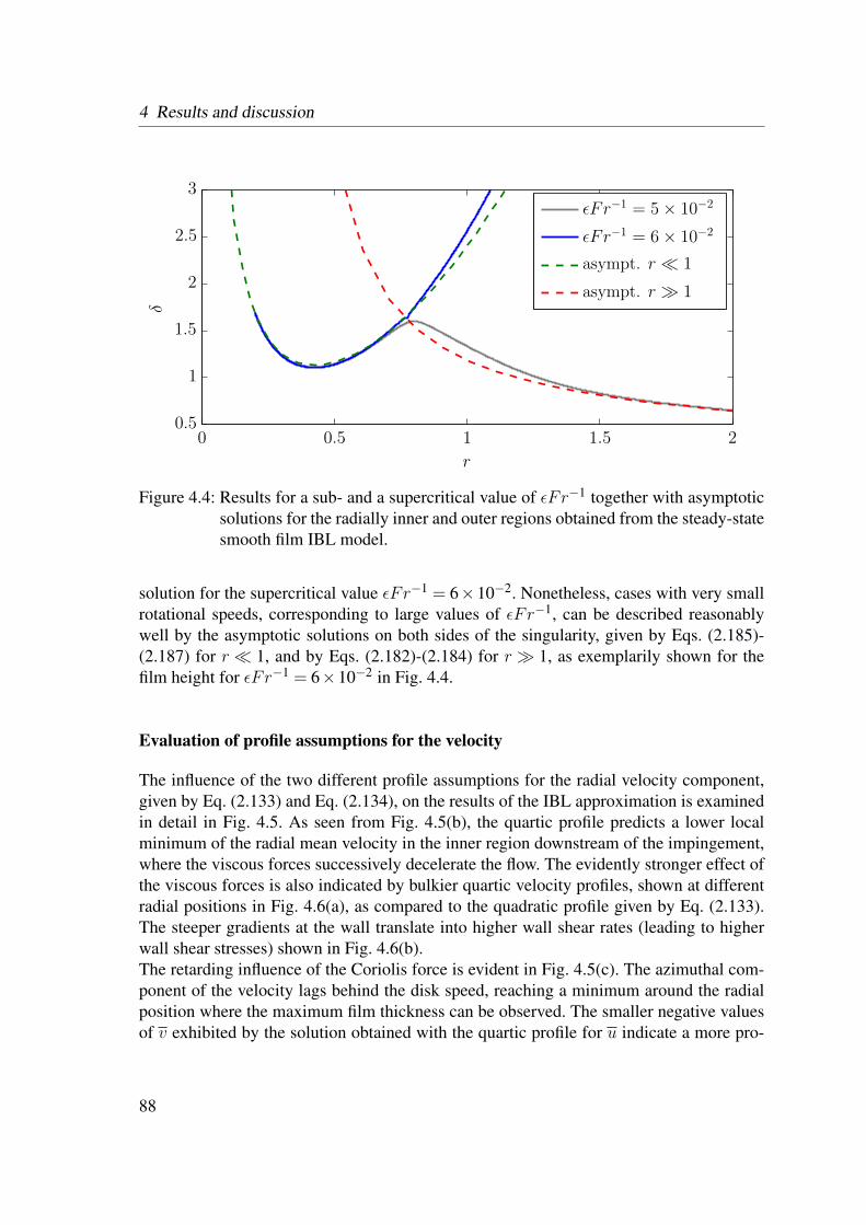
4 Results and discussion
asympt. r ≫ 1
asympt. r ≪ 1
ǫFr−1 = 6× 10⁻²
ǫFr−1 = 5× 10⁻²
δ
r
0 0.5 1 1.5 20.5
1
1.5
2
2.5
3
Figure 4.4: Results for a sub- and a supercritical value of εFr−1 together with asymptoticsolutions for the radially inner and outer regions obtained from the steady-statesmooth film IBL model.
solution for the supercritical value εFr−1 = 6×10⁻². Nonetheless, cases with very smallrotational speeds, corresponding to large values of εFr−1, can be described reasonablywell by the asymptotic solutions on both sides of the singularity, given by Eqs. (2.185)-(2.187) for r 1, and by Eqs. (2.182)-(2.184) for r 1, as exemplarily shown for thefilm height for εFr−1 = 6×10⁻² in Fig. 4.4.
Evaluation of profile assumptions for the velocity
The influence of the two different profile assumptions for the radial velocity component,given by Eq. (2.133) and Eq. (2.134), on the results of the IBL approximation is examinedin detail in Fig. 4.5. As seen from Fig. 4.5(b), the quartic profile predicts a lower localminimum of the radial mean velocity in the inner region downstream of the impingement,where the viscous forces successively decelerate the flow. The evidently stronger effect ofthe viscous forces is also indicated by bulkier quartic velocity profiles, shown at differentradial positions in Fig. 4.6(a), as compared to the quadratic profile given by Eq. (2.133).The steeper gradients at the wall translate into higher wall shear rates (leading to higherwall shear stresses) shown in Fig. 4.6(b).The retarding influence of the Coriolis force is evident in Fig. 4.5(c). The azimuthal com-ponent of the velocity lags behind the disk speed, reaching a minimum around the radialposition where the maximum film thickness can be observed. The smaller negative valuesof v exhibited by the solution obtained with the quartic profile for u indicate a more pro-
88

4.1 Steady-state solutions
nounced retarding effect of the Coriolis force. Accordingly, the assumption of a quarticprofile produces a higher film thickness at radii r > 1 as seen from Fig. 4.5(a).Towards the radial outer boundary of the domain, the differences between the results for thetwo profile assumptions disappear. This can also be mathematically shown in the formula-tion of the profile assumption given by Eq. (2.134). For large radii, the flow is determinedonly by the balance of viscous and centrifugal forces, so that Eq. (2.175) can be rewrittenas
u=β1
β2rδ2 =
13rδ2. (4.3)
Considering steady-state smooth flow in the radially outer region (r 1) the pressuregradient is zero, so that the boundary condition Eq. (2.135) yields κ= r, and Eq. (4.3) canbe rewritten as
u=13κδ2. (4.4)
Using the quartic velocity profile Eq. (2.134), the expression for the surface velocity isgiven by (cf. appendix 2)
uδ =2516u− κδ
2
48. (4.5)
Substituting u= κδ2/3 into Eq. (4.5) yields
κ=2uδδ2 . (4.6)
Introducing this expression for κ into the quartic velocity profile Eq. (2.134), the quarticprofile becomes identical with the quadratic velocity profile, Eq. (2.133). Physically speak-ing, the convergence of both profile assumptions in the radially outer region indicates thevanishing effect of inertia, as this effect can only be reflected by the quartic profile.
Boundary layer assumption (BLA) for the central impingement region
As discussed in Sec. 2.3.4 the IBL approximation with BLA, which considers the devel-opment of boundary layers of the radial and azimuthal velocity components in the radiallyinner region, basically provides a physically more accurate description of the flow, the heatand the species mass transfer near the center.As shown in Fig. 4.7 the predictions of the IBL model using the BLA are very close to thepredictions of the IBL model using the previously discussed developed film assumption(DFA). The boundary layer of the radial velocity component, δr grows very fast due to thehigh shear rates in the impingement region. The boundary layer of the azimuthal velocitycomponent, δφ, reaches the free surface at a radial position farther downstream than δr, asthe growth of δφ is counteracted by the Coriolis force.
89
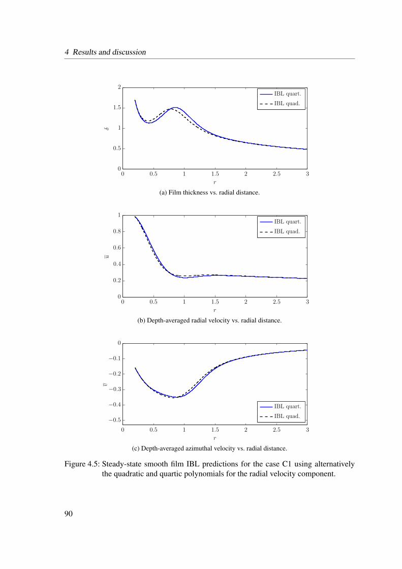
4 Results and discussion
IBL quad.
IBL quart.
δ
r
0 0.5 1 1.5 2 2.5 30
0.5
1
1.5
2
(a) Film thickness vs. radial distance.
IBL quad.
IBL quart.
u
r
0 0.5 1 1.5 2 2.5 30
0.2
0.4
0.6
0.8
1
(b) Depth-averaged radial velocity vs. radial distance.
IBL quad.
IBL quart.
v
r
0 0.5 1 1.5 2 2.5 3
−0.5
−0.4
−0.3
−0.2
−0.1
0
(c) Depth-averaged azimuthal velocity vs. radial distance.
Figure 4.5: Steady-state smooth film IBL predictions for the case C1 using alternativelythe quadratic and quartic polynomials for the radial velocity component.
90

4.1 Steady-state solutions
IBL quad.
IBL quart., r=2
IBL quart., r=0.92
IBL quart., r=0.77
z/δ
u/uδ
0 0.1 0.2 0.3 0.4 0.5 0.6 0.7 0.8 0.9 10
0.2
0.4
0.6
0.8
1
(a) Radial velocity profiles.
IBL quad.
IBL quart.
∂u
∂z
∣ ∣ z=0
r
0 0.5 1 1.5 2 2.5 30
0.5
1
1.5
2
(b) Wall shear rate vs. radial distance.
Figure 4.6: Influence of the two different profile assumptions in the steady-state IBL ap-proximation for the case C1.
91
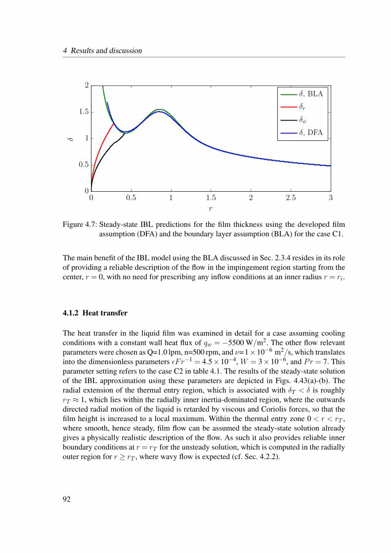
4 Results and discussion
δ, DFA
δφ
δr
δ, BLA
δ
r
0 0.5 1 1.5 2 2.5 30
0.5
1
1.5
2
Figure 4.7: Steady-state IBL predictions for the film thickness using the developed filmassumption (DFA) and the boundary layer assumption (BLA) for the case C1.
The main benefit of the IBL model using the BLA discussed in Sec. 2.3.4 resides in its roleof providing a reliable description of the flow in the impingement region starting from thecenter, r = 0, with no need for prescribing any inflow conditions at an inner radius r = ri.
4.1.2 Heat transfer
The heat transfer in the liquid film was examined in detail for a case assuming coolingconditions with a constant wall heat flux of qw = −5500 W/m2. The other flow relevantparameters were chosen as Q=1.0 lpm, n=500 rpm, and ν=1×10⁻⁶ m2/s, which translatesinto the dimensionless parameters εFr−1 = 4.5×10⁻⁴, W = 3×10⁻⁶, and Pr = 7. Thisparameter setting refers to the case C2 in table 4.1. The results of the steady-state solutionof the IBL approximation using these parameters are depicted in Figs. 4.43(a)-(b). Theradial extension of the thermal entry region, which is associated with δT < δ is roughlyrT ≈ 1, which lies within the radially inner inertia-dominated region, where the outwardsdirected radial motion of the liquid is retarded by viscous and Coriolis forces, so that thefilm height is increased to a local maximum. Within the thermal entry zone 0 < r < rT ,where smooth, hence steady, film flow can be assumed the steady-state solution alreadygives a physically realistic description of the flow. As such it also provides reliable innerboundary conditions at r = rT for the unsteady solution, which is computed in the radiallyouter region for r ≥ rT , where wavy flow is expected (cf. Sec. 4.2.2).
92

4.1 Steady-state solutions
δT
δφ
δr
δ
δ
r
0 0.5 1 1.5 2 2.5 3 3.5 4 4.5 50
0.5
1
1.5
2
(a) Film thickness and thickness of individual boundary layers vs. radial distance.
θ
θδ
θw
θ
r
0 0.5 1 1.5 2 2.5 3 3.5 4 4.5 50
2
4
6
(b) Dimensionless temperature vs. radial distance.
Figure 4.8: IBL predictions for the case C2 assuming steady-state smooth film conditions,Pr = 7.
93

4 Results and discussion
In Fig. 4.43(b) the steady-state IBL predictions for the radial variation of the depth-averageddimensionless temperature θ are shown. The local dimensionless temperatures at the diskand the liquid surface are depicted as well. The liquid surface temperature remains expect-edly at its initial value in the region of the thermal entry for r < rT ≈ 1 and δT < δ, andstarts to increase significantly downstream. For r < rT the radial variation of the wall tem-perature clearly reflects the development of the thermal boundary layer, as θw increasesmarkedly faster than the depth-averaged temperature θ. Further downstream the tempera-ture profiles tend to converge into one curve which indicates that the temperature insidethe film becomes more and more uniform.
To assess the possible effect of the assumption of zero heat flux between the liquid surfaceand the ambient air, the predictions of the steady-state IBL model, using either an adiabaticboundary condition, or a non-adiabatic condition, are compared in Fig. 4.9(a). The far-fieldsolution, which was obtained with the non-adiabatic upper boundary conditions using theNusselt number correlation Eq. (2.194) for the heat transfer coefficient and assuming atypical ambient temperature Ta=25 C, evidently remains fairly close to the predictions ofthe IBL model using an adiabatic upper boundary condition.This observation could also be confirmed by a CFD-based analysis. The numerical resultsobtained from two axisymmetric CFD simulations, using either adiabatic or non-adiabaticsurface conditions, respectively, show no significant differences (Fig. 4.9(b)), although theCFD simulations capture the effects of the surface waviness. As only minor differences areobserved in the results for the temperature variations, the assumption of an adiabatic freesurface appears to be justified.
4.1.3 Species mass transfer
As explained in section 2.4.2 the species mass transfer has to be included in the IBL so-lution in order to model the process of wet chemical surface etching in the limit of largeDamköhler numbers. The operating liquid is assumed as a binary mixture of a primaryetchant component diluted into a chemically inert carrier component. Due to the typicallysmall molecular diffusivities the values of the considered Schmidt numbers are large whencompared against the considered Prandtl numbers for aqueous solutions. Thus, the radialextension of the region, in which a concentration boundary layer has to be distinguished,is considerably larger. This exacerbates the modeling of diffusion controlled etching pro-cesses.
The mass transfer characteristics are examined in detail for a case which is referred toas case C3 in table 4.1. The flow parameters of this case were chosen as Q=1.25 lpm,n=500 rpm, and ν=2.87×10⁻⁶ m2/s, which translates into the dimensionless parameters
94

4.1 Steady-state solutions
IBL asympt. non-adiabatic
IBL steady (adiabatic)
r
〈θw〉
1 2 3 40
1
2
3
4
5
(a) IBL prediction
2D CFD non-adiabatic
2D CFD adiabatic
〈θw〉
r
1 2 3 40
1
2
3
4
5
(b) CFD simulation
Figure 4.9: Dimensionless wall temperature vs. radial distance. Effect of convective heattransport between the liquid surface and the ambient air for the case C2(Ta=25 C) assuming cooling conditions with qw=-5500 W/m2.
95
4 Results and discussion
εFr−1 = 1.03×10⁻³, W = 9.35×10⁻⁶, and Sc= 1196.Fig. 4.10(a) shows the film thickness together with the thickness of the individual boundarylayers, including the concentration boundary layer, δc. The concentration boundary layermonotonously increases up to a local maximum which coincides with the local maximumof the film thickness. In the radial inner region the radial variation of δc evidently followsquite closely the trend of the film height, which indicates that the first term on the RHS ofEq. (2.201) dominates over the second term representing the diffusive transport. Furtherdownstream the common trend disappears as the film height δ decreases, while the con-centration boundary layer δc restarts growing. This opposite trend points at a dominanceof the second (diffusive) term on the RHS of Eq. (2.201).As can be seen from Fig. 4.10(b) the species mass fraction at the free surface, cδ, decreasesfrom its initial value, radially downstream of r = rc ≈ 6, where the concentration bound-ary layer reaches the film surface. It is interesting to note that the also depicted variation ofthe depth-averaged species mass fraction decreases almost linearly with the radial distancethroughout the domain showing no sensitivity to the development of the boundary layers,especially not to δc.
In Fig. 4.11 the radial variation of the Sherwood number is examined. Assuming a third-order polynomial for the profile of the species mass fraction, the Sherwood number is de-termined by the following expression for the dimensionless species mass fraction gradientat the wall
Sh=∂c
∂z
∣∣∣∣z=0
=3cδ2δc .
(4.7)
This implies that for r < rc, where cδ = 1, the diffusive flux at the wall is proportional tothe inverse of the thickness of the concentration boundary layer, i.e.,
∂c
∂z
∣∣∣∣z=0
∝1δc. (4.8)
For r > rc, where cδ decreases, the diffusive flux at the wall is proportional to the ratio
∂c
∂z
∣∣∣∣z=0
∝cδδ. (4.9)
so that it scales with the inverse of the film height. The first proportionality can be clearlyseen from Figs. 4.10(a) and 4.11, where the local minimum in the Sherwood number cor-responds to the local maximum in the thickness of δc, located at a dimensionless radius ofabout r≈ 0.9. The monotonic increase of δc occurring further downstream translates into aslow radial decrease of Sh. Downstream of the radial position r = rc, where the boundarylayer thickness δc reaches the film height δ the Sherwood number exhibits a plateau-likevariation. According to Eq. (4.9) the decrease of cδ starting at r = rc is evidently compen-sated by the decrease of the film height resulting in nearly constant Sherwood numbers.
96

4.1 Steady-state solutions
δc
δφ
δr
δ
δ
r
0 2 4 6 8 100
0.5
1
1.5
(a) Film thickness and thickness of individual boundary layers.
c
cδ
c
r
0 2 4 6 8 100
0.2
0.4
0.6
0.8
11.1
(b) Surface and depth-averaged species mass fraction vs. radial distance.
Figure 4.10: Steady-state IBL solutions for the case C3 including results for the solid-liquid mass transfer in a binary mixture, Sc= 1196.
97

4 Results and discussion
r
∂c
∂z
∣ ∣ z=0
0 2 4 6 8 100
2
4
6
8
10
Figure 4.11: Local Sherwood number for the case C3, Sc= 1196.
Evaluation of profile assumptions for the species mass fraction
In Figs. 4.12-4.13 the influence of the order of the polynomial ansatz function for the pro-file of the species mass fraction is examined. The available boundary conditions allow thecoefficients of a third-order polynomial to be fully determined. If a second-order poly-nomial is considered instead (see appendix 3 for details) the IBL model predicts a fastergrowth of the concentration boundary layer, as can be seen from Fig. 4.12. The fastergrowth of δc immediately follows from the larger concentration gradient of the second-order polynomial at the wall, since
∂
∂z
[cδ
(2z
δc− z
2
δ2c
)]
z=0>
∂
∂z
[cδ
(32z
δc− 1
2z3
δ3c
)]
z=0. (4.10)
The larger gradient results in faster decrease of the bulk concentration, and thus a fastergrowth of δc. Furthermore, the use of a second-order polynomial conflicts with the zero-curvature condition at the wall, Eq. (2.88), as the second derivative reads
∂2
∂z2
[cδ
(2z
δc− z
2
δ2c
)]=−2
cδδ2c. (4.11)
The shortcomings of the second-order polynomial in the near wall region are thereforegreatest in the radially inner region, where the thickness of the concentration boundarylayer is smallest. Radially further downstream the error introduced by the quadratic ap-proximation for the c-profile will decrease as the surface species mass fraction approacheszero, cδ → 0. The faster increase of the thickness of the concentration boundary layer is
98
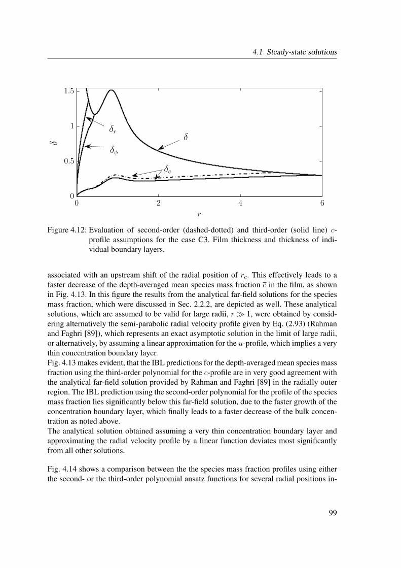
4.1 Steady-state solutions
r
δc
δ
δφ
δr
δ
0 2 4 60
0.5
1
1.5
Figure 4.12: Evaluation of second-order (dashed-dotted) and third-order (solid line) c-profile assumptions for the case C3. Film thickness and thickness of indi-vidual boundary layers.
associated with an upstream shift of the radial position of rc. This effectively leads to afaster decrease of the depth-averaged mean species mass fraction c in the film, as shownin Fig. 4.13. In this figure the results from the analytical far-field solutions for the speciesmass fraction, which were discussed in Sec. 2.2.2, are depicted as well. These analyticalsolutions, which are assumed to be valid for large radii, r 1, were obtained by consid-ering alternatively the semi-parabolic radial velocity profile given by Eq. (2.93) (Rahmanand Faghri [89]), which represents an exact asymptotic solution in the limit of large radii,or alternatively, by assuming a linear approximation for the u-profile, which implies a verythin concentration boundary layer.Fig. 4.13 makes evident, that the IBL predictions for the depth-averaged mean species massfraction using the third-order polynomial for the c-profile are in very good agreement withthe analytical far-field solution provided by Rahman and Faghri [89] in the radially outerregion. The IBL prediction using the second-order polynomial for the profile of the speciesmass fraction lies significantly below this far-field solution, due to the faster growth of theconcentration boundary layer, which finally leads to a faster decrease of the bulk concen-tration as noted above.The analytical solution obtained assuming a very thin concentration boundary layer andapproximating the radial velocity profile by a linear function deviates most significantlyfrom all other solutions.
Fig. 4.14 shows a comparison between the the species mass fraction profiles using eitherthe second- or the third-order polynomial ansatz functions for several radial positions in-
99

4 Results and discussion
IBL second-order poly.
IBL third-order poly.
Ana. r ≫ 1, linear u-profile
Ana. r ≫ 1, quadratic u-profilec
r
0 1 2 3 4 5 6 7 8 9 100
0.2
0.4
0.6
0.8
1
Figure 4.13: Depth-averaged mean species mass fraction vs. radial distance. Steady-stateIBL predictions and analytical far-field solutions (Rahman and Faghri [89])for the case C3, Sc= 1196.
side the liquid film. The analytical far-field solutions are depicted as well. As can be seenfrom Figs. 4.14(a)-(b), there is a good agreement between the IBL solutions and the exactanalytical solution using the quadratic u-profile (Rahman and Faghri [89]), especially inthe near wall region. The IBL predictions for the height of the concentration boundarylayer using the third-order polynomial are in very good agreement with the exact far-fieldsolution, while the IBL results using a second-order polynomial predict a faster increase ofthe concentration boundary layer. At larger radii, where δc = δ, (see Figs. 4.14(c)-(d)), thesecond-order polynomial predicts significantly lower values for the surface species massfraction cδ than the IBL model using the third-order polynomial and the analytical far-field solution, which show good agreement. This behavior is due to the fast growth of theconcentration boundary layer and the resulting more rapid decrease of the species massfraction at the free surface when using the second-order polynomial ansatz function.
Significant deviations from the other solutions are observed in the analytical far-field re-sults using a linear approximation for the radial velocity profile. This analytical solutionexhibits generally lower wall gradients, and a markedly higher thickness of the concentra-tion boundary layer at r = 4. The assumption of a linear velocity profile inside the liquidfilm is evidently inadequate at larger radii, where the analytical far-field solution yieldsthe semi-parabola (2.93), and the radially continuously increasing concentration boundarylayer is not significantly thinner than the film thickness.
100
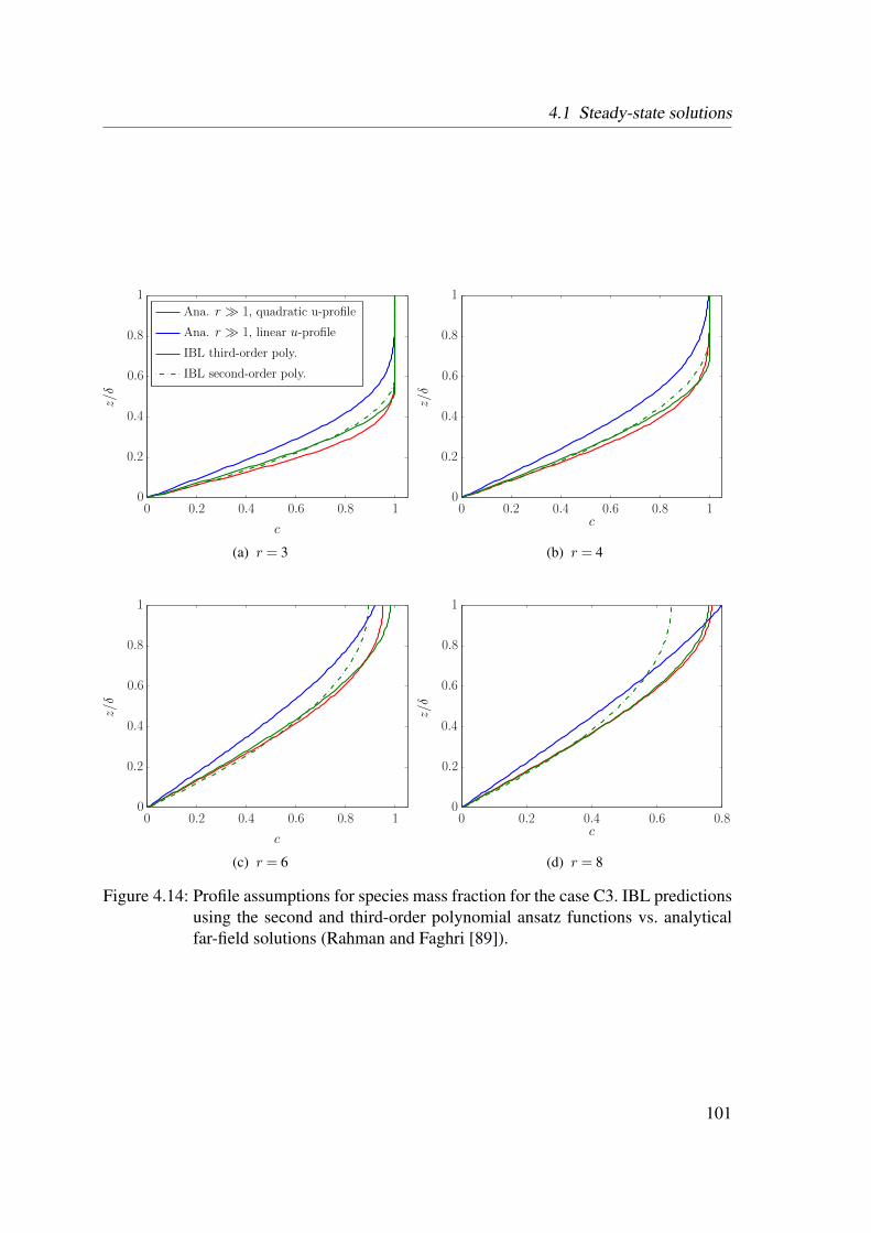
4.1 Steady-state solutions
IBL second-order poly.
IBL third-order poly.
Ana. r ≫ 1, linear u-profile
Ana. r ≫ 1, quadratic u-profile
z/δ
c
0 0.2 0.4 0.6 0.8 10
0.2
0.4
0.6
0.8
1
(a) r = 3
z/δ
c0 0.2 0.4 0.6 0.8 10
0.2
0.4
0.6
0.8
1
(b) r = 4
z/δ
c
0 0.2 0.4 0.6 0.8 10
0.2
0.4
0.6
0.8
1
(c) r = 6
z/δ
c0 0.2 0.4 0.6 0.8
0
0.2
0.4
0.6
0.8
1
(d) r = 8
Figure 4.14: Profile assumptions for species mass fraction for the case C3. IBL predictionsusing the second and third-order polynomial ansatz functions vs. analyticalfar-field solutions (Rahman and Faghri [89]).
101

4 Results and discussion
cδ
c
δc
δφ
δr
δ
δ,c,c δ
r0 2 4 6 8 100
0.5
1
1.5
(a) Sc= 250
δ,c,c δ
r0 2 4 6 8 100
0.5
1
1.5
(b) Sc= 500
δ,c,c δ
r0 2 4 6 8 100
0.5
1
1.5
(c) Sc= 1500
δ,c,c δ
r0 2 4 6 8 100
0.5
1
1.5
(d) Sc= 5000
Figure 4.15: Steady-state IBL results for film thickness, thickness of individual boundarylayers and depth-averaged species mass fraction for varying Schmidt num-bers.
102

4.1 Steady-state solutions
In summary, it can be stated that the predictions of the IBL approximation assuming athird-order polynomial profile for the species mass fraction are generally in very goodagreement with the analytical results, which are obtained by integrating the asymptoticspecies mass transport equation in the far-field for large radii assuming a semi-parabolicvelocity profile.
Effect of the Schmidt number
In Figs. 4.15(a)-(d) the effect of an increase of the Schmidt number on the thickness ofthe concentration boundary layer δc and the depth-averaged mean species mass fraction cis examined. The setting of the hydrodynamical parameters follows again case C3 in table4.1 For the lowest Schmidt number, Sc = 250, the radial extension of the entry length0< r < rc is smallest as expected. The concentration boundary layer increases rapidly andreaches the free surface already at rc≈ 3.3. The depth-averaged mean species mass fractiondecreases fastest with increasing radii and approaches zero in the radially outer region. Anincrease of the Schmidt number results in a shift of rc radially further downstream, ascan be seen from Figs. 4.15(b)-(d). Consistently the radial decrease of the depth-averagedmean species mass fraction becomes slower the larger the Schmidt number.
103

4 Results and discussion
4.2 Effect of wavy flow
In this section the effects of wavy flow conditions on the dynamics and the heat and speciesmass transfer characteristics are analyzed in detail, considering again the three cases whichwere discussed in the analysis of the steady-state smooth film solutions (cf. Tab. 4.1).To validate the predictions of the unsteady IBL model comparisons against results fromnumerical CFD simulations are shown as well.
4.2.1 Hydrodynamics
In Fig. 4.16 the predictions of the unsteady IBL model for the instantaneous radial vari-ations of the film thickness for the case C1, are depicted together with result from anaxisymmetric CFD simulation. In the radially inner region both computational results ex-hibit a smooth film and are in very good agreement. Radially further downstream small dis-turbances are amplified and the generated sequence of small waves with nearly sinusoidal-shape merges into large amplitude waves with steep fronts, preceded by capillary ripples.Good agreement is found for the radial position of wave inception and their evolution radi-ally downstream. The integral method evidently reproduces waves with similar amplitudesand wave lengths as obtained in the axisymmetric CFD simulation. It is interesting to notethat at larger radii the radial extension of the thin film regions, which separate the largeamplitude waves, increases.
2D CFD
IBL unsteady
δ
r
0 0.5 1 1.5 2 2.5 30
0.5
1
1.5
2
Figure 4.16: Instantaneous profiles of the film thickness for the case C1.
104

4.2 Effect of wavy flow
Fig. 4.17 shows the time-averaged profiles of the film thickness predicted by the unsteadyIBL model together with the time-averaged profiles obtained from the axisymmetric CFDsimulation. The asymptotic far-field solution in the limit of large radii, δ = r−2/3, is de-picted as well. In the radial inner region, which is associated with small Ekman numbers,both results exhibit smooth non-wavy film surfaces, so that the shown time-averages donot differ from the instantaneous solution presented in Fig. 4.16. In the wavy region furtherdownstream a very good agreement is seen only between the predictions of the unsteadyIBL model and the predictions of the CFD simulation. In this outer radial region the predic-tion of the asymptotic far-field solution, which basically represents the steady-state smoothfilm IBL solution for large radii, lies well above the time-averaged film height of the un-steady wavy film results. This decrease of the average film thickness associated with wavyflow, which is very well reproduced by the unsteady IBL model, exerts a significant effecton the heat and mass transfer as well, as will be discussed in Sec. 4.2.2 and Sec. 4.2.3,respectively. It is therefore of central importance to capture this salient flow feature whenmodeling the etching process.
2D CFD
Asympt. r ≫ 1
IBL unsteady
〈δ〉
r
0.1 0.6 1.1 1.6 2.1 2.6 3.1 3.50.3
0.7
1.1
1.51.6
Figure 4.17: Time-averaged radial variation of the film thickness for the case C1.
As seen from Fig. 4.18, the time-averaged wall shear rates of the numerical results and thepredictions of the IBL model are also in very good agreement. As a salient feature, theradial wall shear rates of the wavy film lie always well below the prediction of the steady-state smooth-film solution in the radially outer region, where waviness appears. The largestdifference between the predictions of the unsteady IBL model, using either a quartic or aquadratic profile for the radial component of the velocity, is again observed in the inertia
105

4 Results and discussion
dominated radially inner region (r ≤ 2), where, as to be expected, the quartic approxima-tion gives a slightly better estimate for the local wall shear rates when compared againstthe CFD results. Radially further downstream due to the vanishing effect of the inertialforces no significant discrepancies can be observed in the time-averaged predictions of theIBL model using either profile assumptions for the radial component of the velocity.
IBL quad.
IBL quart.
2D CFD
〈∂u
∂z
∣ ∣ z=0〉
r
0 0.5 1 1.5 2 2.5 3 3.50
0.5
1
1.5
2
Figure 4.18: Time-averaged wall shear rates for the case C1.
To examine the profile assumptions, which were required for the depth-averaging in theframework of the IBL model, a comparison with the instantaneous profiles obtained fromthe CFD simulation was carried out. Figs. 4.19 and 4.20 show a comparison between theassumed profile functions and the instantaneous velocity profiles obtained from the CFDanalysis at several radial positions inside a single wave. While the assumed profiles agreevery well with the instantaneous profiles obtained from the CFD simulation at position 1(Fig. 4.19(b)), some deviations from the CFD results are observed upstream of the wavecrests, at positions 2 and 3 (Figs. 4.19(c)-(d)). At position 2, the quartic profile assumptioncomes closer to the CFD prediction, giving a better approximation for the radial componentof the surface velocity. Still, both profile assumptions slightly overpredict the magnitude ofthe numerically obtained result for the surface velocity of the radial velocity component.An opposite tendency can be observed at position 3, where both profile assumptions ofthe IBL model practically coincide. At this position the profile obtained from the CFDsimulation indicates a faster moving layer at the top of the film. At positions 4-6, theanalytically assumed profiles again match the instantaneous velocity profiles obtained withthe CFD simulation very well, as shown in Fig. 4.20.
106
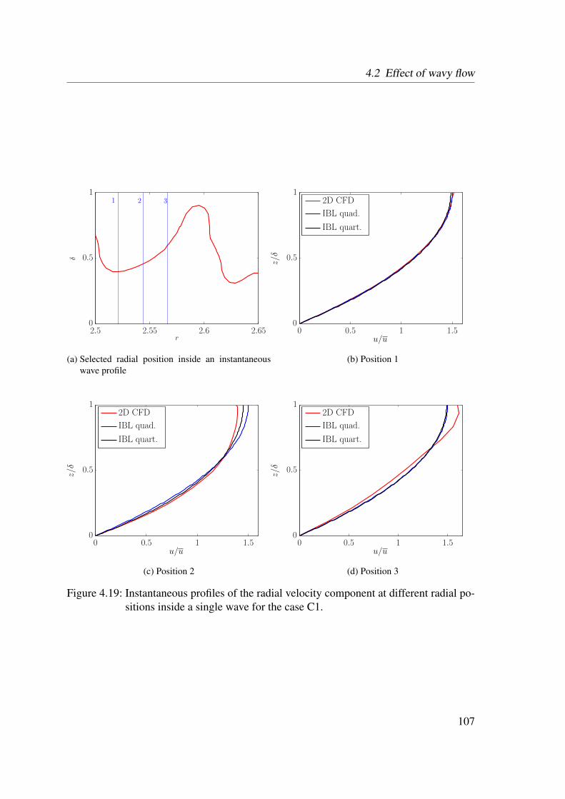
4.2 Effect of wavy flow
δ
r
321
2.5 2.55 2.6 2.650
0.5
1
(a) Selected radial position inside an instantaneouswave profile
IBL quart.
IBL quad.
2D CFD
z/δ
u/u0 0.5 1 1.5
0
0.5
1
(b) Position 1
IBL quart.
IBL quad.
2D CFD
z/δ
u/u0 0.5 1 1.5
0
0.5
1
(c) Position 2
IBL quart.
IBL quad.
2D CFD
z/δ
u/u0 0.5 1 1.5
0
0.5
1
(d) Position 3
Figure 4.19: Instantaneous profiles of the radial velocity component at different radial po-sitions inside a single wave for the case C1.
107
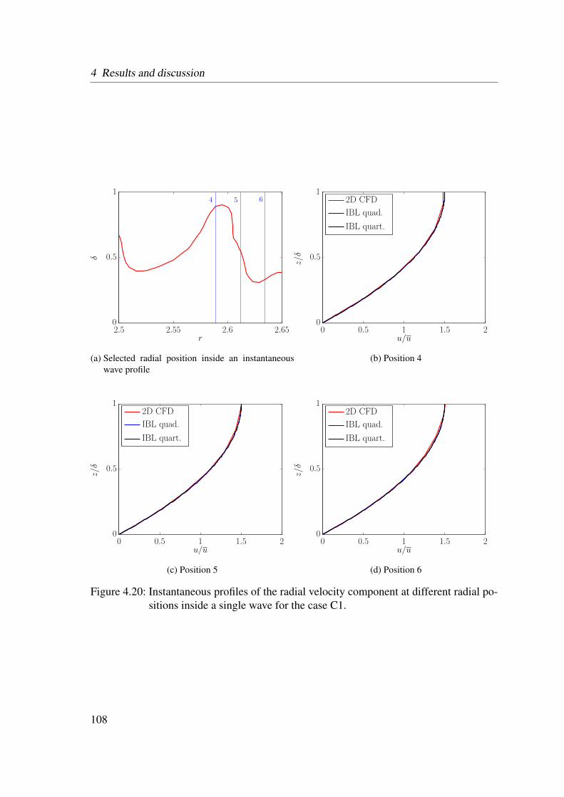
4 Results and discussion
δ
r
654
2.5 2.55 2.6 2.650
0.5
1
(a) Selected radial position inside an instantaneouswave profile
IBL quart.
IBL quad.
2D CFD
z/δ
u/u0 0.5 1 1.5 2
0
0.5
1
(b) Position 4
IBL quart.
IBL quad.
2D CFD
z/δ
u/u0 0.5 1 1.5 2
0
0.5
1
(c) Position 5
IBL quart.
IBL quad.
2D CFD
z/δ
u/u0 0.5 1 1.5 2
0
0.5
1
(d) Position 6
Figure 4.20: Instantaneous profiles of the radial velocity component at different radial po-sitions inside a single wave for the case C1.
108

4.2 Effect of wavy flow
Very importantly, it has to be noted that no significant deviation of the velocity profiles inthe near wall region was observed. This can be considered as a promising aspect, whenextending the IBL approximation to include heat and species mass transfer between theliquid and the disk‘s surface.Concerning the assumption for the profile of the radial velocity it is further noted that thequartic profile (IBL quart.) was used in all IBL results presented in the following, unless itis specifically indicated as quadratic (IBL quad.).
The reduction of the time averaged film height observed in the wavy region can be ex-plained by taking a closer look at the evolution of the instantaneous flow quantities.
In Fig. 4.21(a) the predictions of the unsteady IBL model for the film thickness are depictedtogether with the instantaneous depth-averaged radial velocity u. The shown signals areevidently well in phase, so that the spatial maxima in δ and u coincide. From Fig. 4.21(b)it can be observed that the azimuthal component of the velocity significantly lags behindthe disk speed beneath the wave peaks, while it differs only slightly from the speed of thesolid body rotation in the wave troughs. This indicates the retarding effect of the azimuthalcomponent of the velocity on the flow caused by the Coriolis force, which has alreadybeen pointed out by Matar et al. [79, 90]. Due to this effect waves are propagated at lowerspeeds in rotating films than in corresponding falling films.
In Fig. 4.22 the instantaneous profiles of the film thickness, the radial component of thevelocity at the free surface, and the local wall shear rates are examined in detail. From thenumerical results of the axisymmetric CFD based solution of the Navier-Stokes equations,depicted in Fig. 4.22(a), it is obvious that the variations of the surface velocity are in phasewith to the film thickness, and the values become obviously largest at the wave peaks andsmallest in the wave troughs. Exactly the same behavior is observed in the predictions ofthe IBL model, which are shown in a close-up view in Fig. 4.22(b).The radial position of the maximum in the local wall shear rate predicted by the CFDsimulation is observed in the strongly ascending part on the tail side of the waves, whilethe minima are reached in the wave troughs. In the results of the IBL model local min-ima and maxima in the wall shear rates appear at the same positions relative to the wave.Adomeit and Renz [111] experimentally observed the same positions for the extrema ofthe local wall shear rate relative to the waves in the case of falling liquid films. They ana-lyzed the instantaneous, laminar falling film flow for a large range of Reynolds numbers. Intheir experimental study the maxima in the instantaneous flow rate always coincided withwave crests. Moreover the radial velocity profile was found to be approximately parabolicthroughout the wavy domain. As such these experimental observations for falling films arewell in line with the computational results of the IBL model and the CFD results for theinstantaneous flow on the spinning disk obtained in the present study.
109
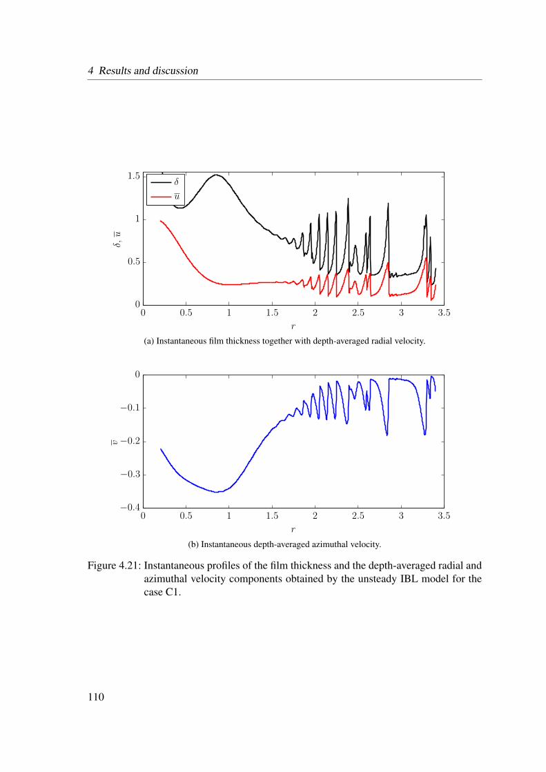
4 Results and discussion
u
δ
δ,u
r
0 0.5 1 1.5 2 2.5 3 3.50
0.5
1
1.5
(a) Instantaneous film thickness together with depth-averaged radial velocity.
v
r
0 0.5 1 1.5 2 2.5 3 3.5−0.4
−0.3
−0.2
−0.1
0
(b) Instantaneous depth-averaged azimuthal velocity.
Figure 4.21: Instantaneous profiles of the film thickness and the depth-averaged radial andazimuthal velocity components obtained by the unsteady IBL model for thecase C1.
110
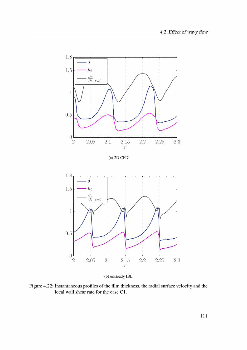
4.2 Effect of wavy flow
∂u∂z
∣∣z=0
uδ
δ
r2 2.05 2.1 2.15 2.2 2.25 2.3
0
0.5
1
1.5
1.8
(a) 2D CFD
∂u∂z
∣∣z=0
uδ
δ
r2 2.05 2.1 2.15 2.2 2.25 2.3
0
0.5
1
1.5
1.8
(b) unsteady IBL
Figure 4.22: Instantaneous profiles of the film thickness, the radial surface velocity and thelocal wall shear rate for the case C1.
111

4 Results and discussion
t
u
δ
0 0.1 0.2 0.3 0.4 0.5 0.6 0.70
0.2
0.4
0.6
0.8
1
Figure 4.23: IBL predictions for the case C2. Temporal evolution of film thickness andradial velocity at r= 3. Dashed horizontal lines: time-averaged predictions ofunsteady IBL model. Dotted horizontal lines: steady-state smooth film IBLpredictions.
A closer look at the evolution of the instantaneous flow quantities in time is shown inFig. 4.23 for the case C2. This particular case will also be considered in the next sec-tion, where the effect of the wavy flow on the heat transfer is examined. In Fig. 4.23 theevolution of the instantaneous film thickness is plotted together with the evolutions of theinstantaneous depth-averaged radial velocity u, at a fixed radial position r = 3. The cor-responding time-averaged mean values of the unsteady and the steady-state smooth filmsolutions are indicated by the horizontal dashed and dotted lines, respectively. The showntime signals make evident again that the depth-averaged radial velocity is in phase with thefilm height. It can be inferred from the coincidence of the maxima/minima in δ and u thata considerable part of the liquid volume passes the disk in shape of fast moving solitarywaves. The comparatively longer periods associated with a very thin film coverage occur-ring between the passage of the large waves effectively lead to smaller time-averaged filmheights.
The present findings based on the temporal evolution of the relevant dynamic quantitiespredicted by the unsteady IBL model are again supported by numerical results obtainedfrom a CFD simulation. As seen from Fig. 4.24, the different time signals from the CFDanalysis feature the same wave pattern as it was obtained from the unsteady IBL solution.
112

4.2 Effect of wavy flow
t
u
δ
0 0.1 0.2 0.3 0.4 0.5 0.6 0.70
0.2
0.4
0.6
0.8
1
Figure 4.24: CFD results for the case C2. Temporal evolution of film thickness and depth-averaged radial velocity at r= 3. Dashed horizontal lines: time-averaged pre-dictions of unsteady IBL model. Dotted horizontal lines: steady-state smoothfilm IBL predictions.
Summing up, it can be stated that the present unsteady IBL model is capable to capture theessential instantaneous hydrodynamic features of the thin film flow at a high descriptivelevel.
4.2.2 Heat transfer
Fig. 4.25(a) shows the time-averaged profiles of the film thickness for the case C2 asobtained from the IBL model using the steady-state and the unsteady formulation, as wellas the results of the axisymmetric CFD simulation. In the radial inner region for r / 2,which is associated with small Ekman numbers Ek / 3, both the steady and the unsteadyIBL solutions exhibit smooth non-wavy film surfaces. This behavior is also shown by theCFD results. In the wavy region further downstream for r > 2 and larger values of thelocal Ekman number the steady IBL model essentially produces the variation of the filmthickness in the asymptotic limit of large radii, δ = r−2/3, which again evidently lies wellabove the time-averaged film height of the unsteady wavy film results. This decrease ofthe time-average film thickness associated with wavy flow is again very well reproducedby the unsteady IBL model.The radial variations of the dimensionless wall temperature predicted by the unsteady IBLmodel and the axisymmetric CFD simulation clearly reflect the effect of waviness as well,
113

4 Results and discussion
as it is seen from Fig. 4.25(b). Both the predictions of the unsteady IBL model and theCFD show in good agreement an enhanced radial increase of 〈θw〉 in the wavy region (r >2.5). In contrast, the smooth film solution of the steady IBL model predicts a considerablyslower radial increase of 〈θw〉 resulting in markedly lower values for the dimensionlesswall temperature in the outer radial region, associated with local Ekman numbers Ek ' 3and surface waves.According to the definition (2.53) a higher dimensionless wall temperature corresponds toa lower wall temperature Tw, when cooling conditions, prescribed in terms of a negativewall heat flux qw, are assumed. Thus, the unsteady IBL solution, which captures the for-mation and propagation of the surface waves, evidently produces on average lower walltemperatures as compared to the steady-state smooth film results. Analogously, in the caseof a heated film, associated with a positive wall heat flux (qw > 0) in the definition (2.53),the wall temperature in the wavy film solution would be higher.
The increase of the time-averaged dimensionless wall temperature θw, observed in thewavy region can again be explained by taking a closer look at the evolution of the instan-taneous flow and thermal quantities in time.Fig. 4.26(a) shows the evolution of the instantaneous film thickness plotted together withthe evolutions of the instantaneous depth-averaged radial velocity u and the depth-averageddimensionless temperature θ, at a fixed radial position r = 3. The corresponding time-averaged mean values of the unsteady and the steady-state smooth film solutions are indi-cated by the horizontal dashed and dotted lines, respectively. The temporal maxima/minimain δ and u are found again to coincide. Furthermore, the time signals of the shown dimen-sionless temperatures are all in phase with the film height and the velocity as well, but herethe minima in the θ-values coincide with the maxima in δ, or u, and vice versa. Assumingheated film flow conditions (qw > 0), this implies that during the periods with small filmheights and slow radial motion the temperature of the thin liquid layer is increased veryfast by the heating from below. The temperature inside the liquid also becomes more uni-form as seen from the converging tendency of the individual θ-signals (Fig. 4.26(a)). Thecomparatively long periods associated with higher temperature levels of the liquid finallyexplains the increased temporal averages of the non-dimensional wall temperature θw ob-tained for the unsteady IBL solution in the wavy region.
The present findings based on the temporal evolution of the relevant dynamic and thermalquantities are also supported by numerical results obtained from a CFD simulation. Asseen from Fig. 4.26(b), the different time signals show the same behavior, as it was seen inthe results of the unsteady IBL solution.
An assessment of the instantaneous velocity and temperature profiles at several time in-stants inside a single wave is shown in Figs. 4.27-4.28. The velocity profiles are normal-ized with the corresponding absolute value of the surface velocity, so that the signs of the
114
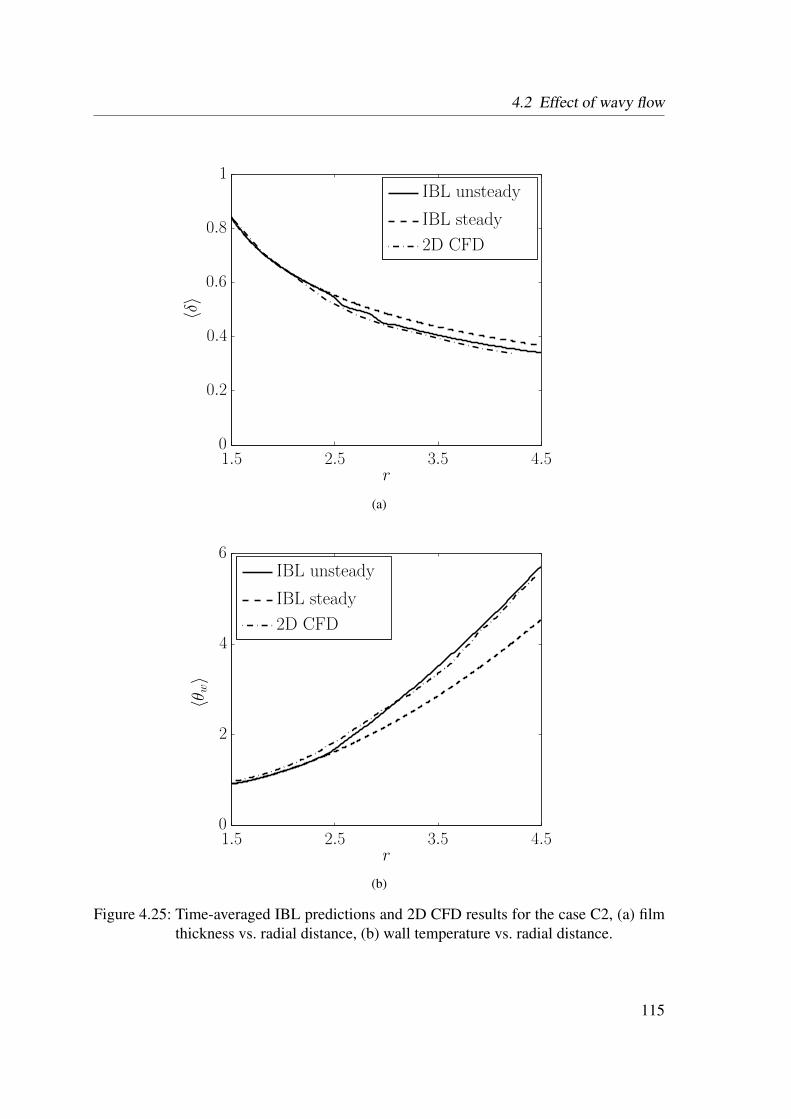
4.2 Effect of wavy flow
2D CFD
IBL steady
IBL unsteady〈δ〉
r1.5 2.5 3.5 4.50
0.2
0.4
0.6
0.8
1
(a)
2D CFD
IBL steady
IBL unsteady
〈θw〉
r1.5 2.5 3.5 4.50
2
4
6
(b)
Figure 4.25: Time-averaged IBL predictions and 2D CFD results for the case C2, (a) filmthickness vs. radial distance, (b) wall temperature vs. radial distance.
115

4 Results and discussion
t
θw θ
u
θδ
δ(a)
(b)
0 0.2 0.4 0.61.8
2
2.2
2.4
2.6
0
0.2
0.4
0.60.7
(a) IBL model
t
θ
uδ
0 0.2 0.4 0.60
1
2
3
(b) 2D CFD
Figure 4.26: Temporal evolution of film thickness, depth-averaged radial velocity, anddepth-averaged temperature at r= 3 for the case C2. Dashed horizontal lines:time-averaged predictions of unsteady IBL model. Dotted horizontal lines:steady-state smooth film IBL predictions.
116
4.2 Effect of wavy flow
normalized velocities indicate the orientation of the motion at the surface relative to therotating disk. One should also bear in mind that in the wavy region the maximum valuesof the relative azimuthal and wall normal velocity components are at least one order ofmagnitude smaller than the radial surface velocities. The dashed curves always refer to theprofiles of the IBL model, where the radial and the azimuthal velocity components are de-termined by the assumed quartic polynomials, Eqs. (2.134) and (2.136), respectively, andthe vertical wall normal velocity is computed from Eq. (2.142).At the instants of time associated with the passage of a wave trough, Figs. 4.27(b)-(c), afairly good agreement between the assumed velocity profiles and the instantaneous pro-files obtained from the CFD simulation is found. Moreover, also the assumed third-orderpolynomial for the temperature reproduces very well the temperature distribution obtainedfrom the CFD results. Between time instant 2 and 3 the sign of the vertical surface velocityswitches from negative to positive. Within this short interval of time (see e.g. Fig. 4.27(d))a steep wave front passes by, and all profiles associated with the IBL model significantlydeviate from the corresponding CFD results. Here the CFD results suggest a two-layeredflow with a fast moving surface layer and a slowly moving bottom layer. These short pe-riods associated with the passage of steep wave fronts make the limitations of the currentIBL model, or rather its profile assumptions, evident. Aside from these discrepancies, ascan be observed from Fig. 4.28, a very good agreement between the IBL profiles and theinstantaneous profiles obtained from the CFD simulation is found again at instants 4-6.These instants of time refer to the passage of the descending tail side parts of the waves.
Dynamically speaking, the observed wave propagation is driven by the centrifugal force,which pushes the liquid towards the front faces of the waves crests. In effect, as indicatedby the sign of the vertical component of the surface velocity, the liquid motion is directedupwards when the steep front faces of the waves are passing, while it is directed down-wards otherwise. Thus, the action of the centrifugal force effectively steepens the wavesresulting in the formation of large solitary waves, which are separated by relatively largethin film regions. The wave crests are moving relatively faster than the liquid in the bottomlayer as indicated by the S-shaped profile seen in Fig. 4.27(d).
Since the deviations of the profiles used for the IBL model from the corresponding CFDresults occur only during comparatively short periods of time, the predictions of the presentunsteady IBL model still provide a very reliable description of the wavy film flow includ-ing heat transfer. Nonetheless, the assumed profile functions required by the IBL approachstill represent an important limitation of this model when considering wavy flow.
117
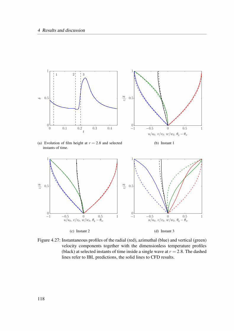
4 Results and discussion
321
δ
t0 0.1 0.2 0.3 0.4
0
0.5
1
(a) Evolution of film height at r = 2.8 and selectedinstants of time.
z/δ
u/uδ, v/vδ, w/wδ, θq − θw
−1 −0.5 0 0.5 10
0.5
1
(b) Instant 1
z/δ
u/uδ, v/vδ, w/wδ, θq − θw−1 −0.5 0 0.5 10
0.5
1
(c) Instant 2
z/δ
u/uδ, v/vδ, w/wδ, θq − θw−1 −0.5 0 0.5 10
0.5
1
(d) Instant 3
Figure 4.27: Instantaneous profiles of the radial (red), azimuthal (blue) and vertical (green)velocity components together with the dimensionless temperature profiles(black) at selected instants of time inside a single wave at r= 2.8. The dashedlines refer to IBL predictions, the solid lines to CFD results.
118

4.2 Effect of wavy flow
654
δ
t0 0.1 0.2 0.3 0.4
0
0.5
1
(a) Evolution of film height at r = 2.8 and selectedinstants of time.
z/δ
u/uδ, v/vδ, w/wδ, θq − θw−1 −0.5 0 0.5 10
0.5
1
(b) Instant 4
z/δ
u/uδ, v/vδ, w/wδ, θq − θw−1 −0.5 0 0.5 10
0.5
1
(c) Instant 5
z/δ
u/uδ, v/vδ, w/wδ, θq − θw−1 −0.5 0 0.5 10
0.5
1
(d) Instant 6
Figure 4.28: Instantaneous profiles of the radial (red), azimuthal (blue) and vertical (green)velocity components together with the dimensionless temperature profiles(black) at selected instants of time inside a single wave at r= 2.8. The dashedlines refer to IBL predictions, the solid lines to CFD results.
119

4 Results and discussion
4.2.3 Species mass transfer
To assess the predictive capability of the unsteady IBL model for species mass transfer inwavy films the case referred to as C3 in table 4.1 was considered. Fig. 4.29(a) shows theIBL predictions for the instantaneous film thickness and the thickness of the concentrationboundary layer, together with the corresponding time-averaged results denoted by the redlines. The corresponding results for the film thickness and the height of the concentrationboundary layer of a CFD simulation, which was carried out as well to validate the resultsof the unsteady IBL solution, are shown in Fig. 4.29(b). In the radially inner region, theCFD results as well as the predictions of the IBL model exhibit a smooth film. The time-averaged film thickness and the thickness of the concentration boundary layer remain closeto the steady-state solution in the region associated with r / 2, and both computational re-sults agree well with each other. Radially further downstream the formation of nonlinearwaves on the film surface leads to strong variations of the thickness of the concentra-tion boundary layer in the predictions of the IBL model. With growing amplitudes of thesurface waves the local maxima in the thickness of the concentration boundary layer in-crease as well. As a consequence, a fast radial increase of the time-averaged concentrationboundary layer is observed in the region 2.5 / r / 3. In contrast, the time-averaged con-centration boundary layer thickness increases notably more slowly in the CFD results inthis interval. Radially further downstream the time-averaged thickness of the concentrationboundary layer predicted by the IBL model follows closely the trend of the time-averagedfilm height.
Fig. 4.30 shows the time-averaged results for the radial variation of the film thickness,the surface species mass fraction, and the Sherwood number. While for the time-averagedfilm thickness again very good agreement between the predictions of the unsteady IBLmodel and the CFD results is found, the time-averaged results for the species transportdiffer significantly. The IBL model predicts a much faster decrease of the species massfraction at the surface from its initial value in the radially outer region. Moreover, the pre-dictions of the unsteady IBL model show a very fast radial decrease of the time-averagednon-dimensional concentration gradient at the wall represented by the Sherwood numberin comparison to the steady-state smooth film solution. This behavior results from the sud-den increase of the thickness of the concentration boundary layer as can be immediatelyseen from Eq. (4.7). In contrast to the unsteady IBL predictions the time-averaged localSherwood number of the CFD solution remains almost constant in this region. In the outerradial region they even come very close to the results of the steady-state smooth film IBLmodel.
The inability of the present unsteady IBL model to capture correctly the effect of wavinesson the species transport can be explained by taking a closer look at the evolution of the in-stantaneous flow quantities and the assumed profile functions for the velocity componentsand the species mass fraction in time.
120

4.2 Effect of wavy flow
δ
r
δc
δ
0 0.5 1 1.5 2 2.5 3 3.5 4 4.5 50
0.5
1
1.5
2
(a) IBL model
δ
r
δc
δ
0 0.5 1 1.5 2 2.5 3 3.5 4 4.5 50
0.5
1
1.5
2
(b) 2D CFD
Figure 4.29: Instantaneous film and concentration boundary layer thickness (black lines)together with the corresponding time-averages (red lines) for the case C3.
121
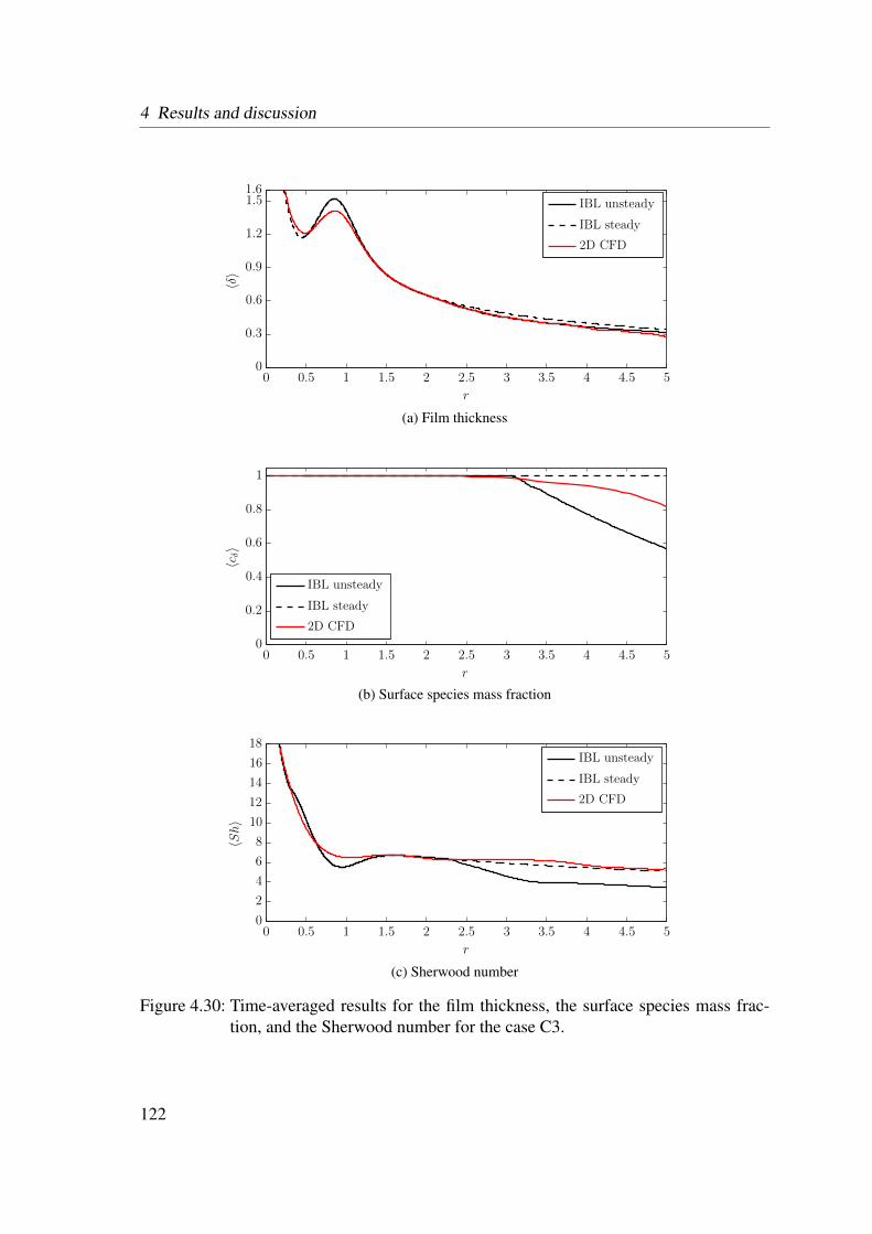
4 Results and discussion
2D CFD
IBL steady
IBL unsteady
〈δ〉
r
0 0.5 1 1.5 2 2.5 3 3.5 4 4.5 50
0.3
0.6
0.9
1.2
1.51.6
(a) Film thickness
2D CFD
IBL steady
IBL unsteady
〈cδ〉
r
0 0.5 1 1.5 2 2.5 3 3.5 4 4.5 50
0.2
0.4
0.6
0.8
1
(b) Surface species mass fraction
2D CFD
IBL steady
IBL unsteady
〈Sh〉
r
0 0.5 1 1.5 2 2.5 3 3.5 4 4.5 50
2
4
6
8
10
12
14
16
18
(c) Sherwood number
Figure 4.30: Time-averaged results for the film thickness, the surface species mass frac-tion, and the Sherwood number for the case C3.
122
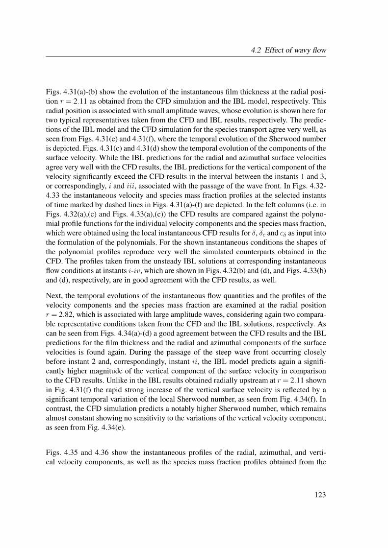
4.2 Effect of wavy flow
Figs. 4.31(a)-(b) show the evolution of the instantaneous film thickness at the radial posi-tion r = 2.11 as obtained from the CFD simulation and the IBL model, respectively. Thisradial position is associated with small amplitude waves, whose evolution is shown here fortwo typical representatives taken from the CFD and IBL results, respectively. The predic-tions of the IBL model and the CFD simulation for the species transport agree very well, asseen from Figs. 4.31(e) and 4.31(f), where the temporal evolution of the Sherwood numberis depicted. Figs. 4.31(c) and 4.31(d) show the temporal evolution of the components of thesurface velocity. While the IBL predictions for the radial and azimuthal surface velocitiesagree very well with the CFD results, the IBL predictions for the vertical component of thevelocity significantly exceed the CFD results in the interval between the instants 1 and 3,or correspondingly, i and iii, associated with the passage of the wave front. In Figs. 4.32-4.33 the instantaneous velocity and species mass fraction profiles at the selected instantsof time marked by dashed lines in Figs. 4.31(a)-(f) are depicted. In the left columns (i.e. inFigs. 4.32(a),(c) and Figs. 4.33(a),(c)) the CFD results are compared against the polyno-mial profile functions for the individual velocity components and the species mass fraction,which were obtained using the local instantaneous CFD results for δ, δc and cδ as input intothe formulation of the polynomials. For the shown instantaneous conditions the shapes ofthe polynomial profiles reproduce very well the simulated counterparts obtained in theCFD. The profiles taken from the unsteady IBL solutions at corresponding instantaneousflow conditions at instants i-iv, which are shown in Figs. 4.32(b) and (d), and Figs. 4.33(b)and (d), respectively, are in good agreement with the CFD results, as well.
Next, the temporal evolutions of the instantaneous flow quantities and the profiles of thevelocity components and the species mass fraction are examined at the radial positionr= 2.82, which is associated with large amplitude waves, considering again two compara-ble representative conditions taken from the CFD and the IBL solutions, respectively. Ascan be seen from Figs. 4.34(a)-(d) a good agreement between the CFD results and the IBLpredictions for the film thickness and the radial and azimuthal components of the surfacevelocities is found again. During the passage of the steep wave front occurring closelybefore instant 2 and, correspondingly, instant ii, the IBL model predicts again a signifi-cantly higher magnitude of the vertical component of the surface velocity in comparisonto the CFD results. Unlike in the IBL results obtained radially upstream at r = 2.11 shownin Fig. 4.31(f) the rapid strong increase of the vertical surface velocity is reflected by asignificant temporal variation of the local Sherwood number, as seen from Fig. 4.34(f). Incontrast, the CFD simulation predicts a notably higher Sherwood number, which remainsalmost constant showing no sensitivity to the variations of the vertical velocity component,as seen from Fig. 4.34(e).
Figs. 4.35 and 4.36 show the instantaneous profiles of the radial, azimuthal, and verti-cal velocity components, as well as the species mass fraction profiles obtained from the
123

4 Results and discussion
31 2 4
δ
t
0 0.1 0.2 0.3 0.40
0.5
1
(a) 2D CFD: film height at r = 2.11.
ivi iiiii
δ
t0 0.2 0.4
0
0.5
1
(b) IBL model: film height at r = 2.11.
wδ
vδ
uδ
surfacevelocity
t0 0.1 0.2 0.3 0.4
−1
0
1
2
(c) 2D CFD: surface velocity
wδ
vδ
uδ
surfacevelocity
t
0 0.2 0.4−1
0
1
2
(d) IBL model: surface velocity
Sh
t0 0.1 0.2 0.3 0.4
5
6
7
8
(e) 2D CFD: Sherwood number
Sh
t0 0.2 0.4
5
6
7
8
(f) IBL model: Sherwood number
Figure 4.31: Evolution of the film height, the surface velocity, and the Sherwood numberat r = 2.11. Vertical dashed lines indicate selected instants of time.
124

4.2 Effect of wavy flow
c
w/wδ
v/vδ
u/uδ
z/δ
u/uδ, v/vδ, w/wδ, c−1 −0.5 0 0.5 10
0.5
1
(a) 2D CFD, instant of time 1
c
w/wδ
v/vδ
u/uδ
z/δ
u/uδ, v/vδ, w/wδ, c−1 −0.5 0 0.5 10
0.5
1
(b) IBL model, instant of time i
c
w/wδ
v/vδ
u/uδ
z/δ
u/uδ, v/vδ, w/wδ, c
−1 −0.5 0 0.5 10
0.5
1
(c) 2D CFD, instant of time 2
c
w/wδ
v/vδ
u/uδ
z/δ
u/uδ, v/vδ, w/wδ, c−1 −0.5 0 0.5 10
0.5
1
(d) IBL model, instant of time ii
Figure 4.32: Instantaneous profiles of the radial, azimuthal, and vertical velocity compo-nents together with the species mass fraction profile at selected instants oftime inside a single wave at r= 2.11 for the case C3. The dashed-dotted linesrefer to the results of the unsteady IBL model, the solid lines to the simu-lated profiles of the CFD, and the dashed lines refer to the polynomial profilefunctions evaluated with the CFD results as input.
125
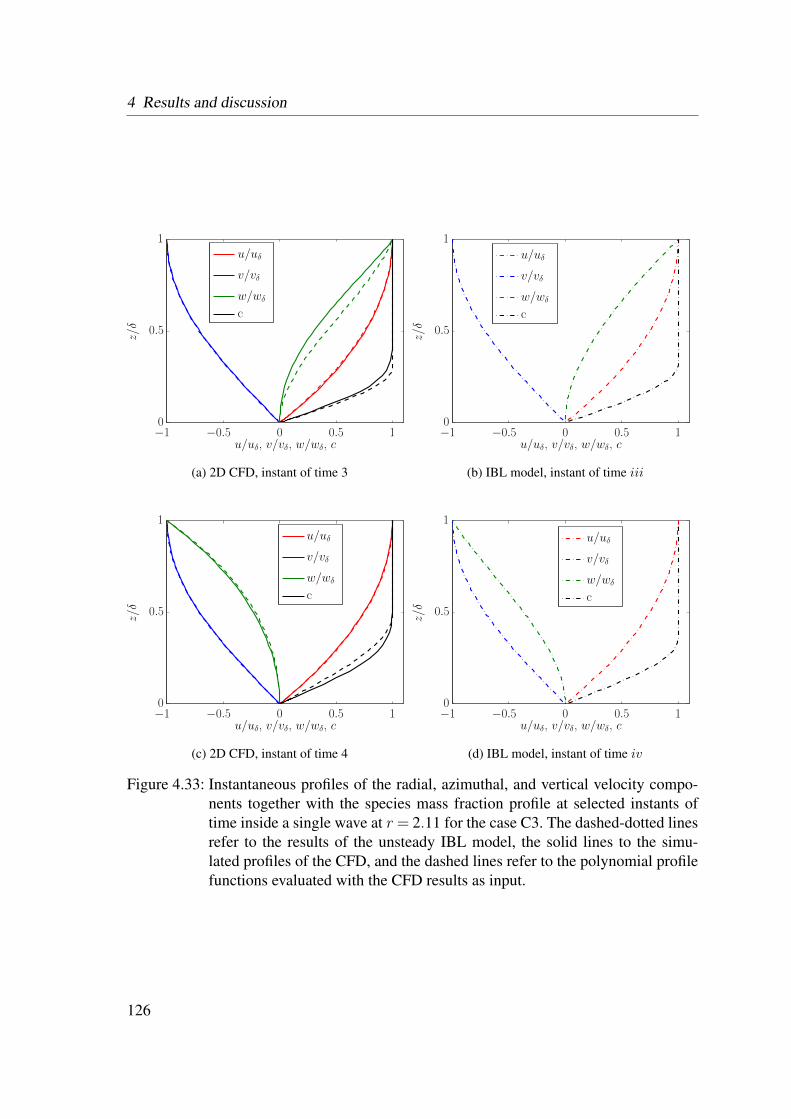
4 Results and discussion
c
w/wδ
v/vδ
u/uδ
z/δ
u/uδ, v/vδ, w/wδ, c−1 −0.5 0 0.5 10
0.5
1
(a) 2D CFD, instant of time 3
c
w/wδ
v/vδ
u/uδ
z/δ
u/uδ, v/vδ, w/wδ, c−1 −0.5 0 0.5 10
0.5
1
(b) IBL model, instant of time iii
c
w/wδ
v/vδ
u/uδ
z/δ
u/uδ, v/vδ, w/wδ, c−1 −0.5 0 0.5 10
0.5
1
(c) 2D CFD, instant of time 4
c
w/wδ
v/vδ
u/uδ
z/δ
u/uδ, v/vδ, w/wδ, c−1 −0.5 0 0.5 10
0.5
1
(d) IBL model, instant of time iv
Figure 4.33: Instantaneous profiles of the radial, azimuthal, and vertical velocity compo-nents together with the species mass fraction profile at selected instants oftime inside a single wave at r= 2.11 for the case C3. The dashed-dotted linesrefer to the results of the unsteady IBL model, the solid lines to the simu-lated profiles of the CFD, and the dashed lines refer to the polynomial profilefunctions evaluated with the CFD results as input.
126
4.2 Effect of wavy flow
CFD and the IBL solution at four selected instants of time within the interval shown inFig. 4.34. While a fairly good agreement between the CFD results and the polynomialprofile assumptions is generally found for the radial and azimuthal velocity components,large deviations are observed for the vertical component of the velocity, especially at theinstant 2 associated with the passage of the peak of the wave. At the instants of time 3 and4, and correspondingly, iii and iv, i.e., after the passage of the wave peak, a fairly goodagreement with the CFD results is observed again for all components. This observationapplies to the polynomial functions using the CFD solution as input, as well as those takenfrom the unsteady IBL solution.Marked deviations in the w-profiles do not only appear during the passage of the wavepeaks. They were also observed, less pronounced, after the passage of the large solitarywaves, as seen from Fig. 4.37 showing conditions obtained further downstream at r= 4.23.As for the mass transfer, the simulated profiles for the species mass concentration exhibitalways a higher wall gradient than the polynomial functions. This explains the higher levelof the local Sherwood number predicted by the CFD seen from Figs. 4.34(e)-(f), which isalso reflected by the radial variations of the time-averaged Sherwood number in the outerwavy region shown in Fig. 4.30(c).
The detailed discussion of the velocity profiles above suggests that the observed deficitsof the unsteady IBL model in the description of the species mass transfer can be mainlyattributed to some inherent limitations of the assumed profile functions required by thedepth-averaging. These limitations become most evident in the discrepancies observedfor the w-profiles, which are implicitly determined by the polynomials assumed for theradial and azimuthal velocities. According to the definition of the profiles for u, v, c, andimplicitly, for w, they essentially scale with the thickness of the film δ, so that a strongtemporal variation of the height of the liquid surface in the wavy region practically rescalesthe whole profiles down to the wall while leaving the prescribed shape of the polynomialsunchanged. As a consequence, the onset of surface waviness always leads to a very fastincrease of the thickness of the concentration boundary layer, which in turn leads to amarked radial decrease of the time-averaged Sherwood number due to Sh ∝ 1/δc, as seenfrom Fig. 4.30(c). This inherent feature is especially problematic for the here consideredhigh Schmidt number, Sc = 1196. High Schmidt numbers imply very thin concentrationboundary layers, which are expected to be less sensitive to the unsteady motion of theliquid in the wavy surface layer, than it is inherently imposed by the polynomial profilefunctions.
The present reasoning is also supported by a simple test assuming quasi-steady “frozenwaves“ by neglecting the transient term in the kinematic boundary condition, Eq. (2.77),such that
wδ = uδ∂δ
∂r. (4.12)
Using this quasi-steady formulation in the depth-averaged mass transport equation (2.163)
127

4 Results and discussion
4321
δ
t0 0.1 0.2 0.3 0.4 0.5
0
0.5
1
(a) 2D CFD: film height at r = 2.82
iviiiiii
δ
t0 0.1 0.2 0.3 0.4 0.50
0.5
1
(b) IBL model: film height at r = 2.82
wδ
vδ
uδ
surfacevelocity
t
0 0.1 0.2 0.3 0.4 0.5−5
0
5
10
15
(c) 2D CFD: surface velocity
wδ
vδ
uδ
surfacevelocity
t0 0.1 0.2 0.3 0.4 0.5
−5
0
5
10
15
(d) IBL model: surface velocity
Sh
t0 0.1 0.2 0.3 0.4 0.50
2
4
6
(e) 2D CFD: Sherwood number
Sh
t0 0.1 0.2 0.3 0.4 0.50
2
4
6
(f) IBL model: Sherwood number
Figure 4.34: Evolution of the film height, the surface velocity, and the Sherwood numberat r = 2.82. Vertical dashed lines indicate selected instants of time.
128

4.2 Effect of wavy flow
c
w/wδ
v/vδ
u/uδ
z/δ
u/uδ, v/vδ, w/wδ, c−1 −0.5 0 0.5 10
0.5
1
(a) 2D CFD, time instant 1
c
w/wδ
v/vδ
u/uδ
z/δ
u/uδ, v/vδ, w/wδ, c
−1 −0.5 0 0.5 10
0.5
1
(b) IBL model, time instant i
c
w/wδ
v/vδ
u/uδ
z/δ
u/uδ, v/vδ, w/wδ, c−1 −0.5 0 0.5 10
0.5
1
(c) 2D CFD, time instant 2
c
w/wδ
v/vδ
u/uδ
z/δ
u/uδ, v/vδ, w/wδ, c
−1 −0.5 0 0.5 10
0.5
1
(d) IBL model, time instant ii
Figure 4.35: Instantaneous profiles of the radial, azimuthal, and vertical velocity compo-nents together with the species mass fraction profile at selected instants oftime inside a single wave at r= 2.82 for the case C3. The dashed-dotted linesrefer to the results of the unsteady IBL model, the solid lines to the simu-lated profiles of the CFD, and the dashed lines refer to the polynomial profilefunctions evaluated with the CFD results as input.
129

4 Results and discussion
c
w/wδ
v/vδ
u/uδ
z/δ
u/uδ, v/vδ, w/wδ, c−1 −0.5 0 0.5 10
0.5
1
(a) D CFD, time instant 3
c
w/wδ
v/vδ
u/uδ
z/δ
u/uδ, v/vδ, w/wδ, c
−1 −0.5 0 0.5 10
0.5
1
(b) IBL model, time instant iii
c
w/wδ
v/vδ
u/uδ
z/δ
u/uδ, v/vδ, w/wδ, c−1 −0.5 0 0.5 10
0.5
1
(c) 2D CFD, time instant 4
c
w/wδ
v/vδ
u/uδ
z/δ
u/uδ, v/vδ, w/wδ, c
−1 −0.5 0 0.5 10
0.5
1
(d) IBL model, time instant iv
Figure 4.36: Instantaneous profiles of the radial, azimuthal, and vertical velocity compo-nents together with the species mass fraction profile at selected instants oftime inside a single wave at r= 2.82 for the case C3. The dashed-dotted linesrefer to the results of the unsteady IBL model, the solid lines to the simu-lated profiles of the CFD, and the dashed lines refer to the polynomial profilefunctions evaluated with the CFD results as input.
130

4.2 Effect of wavy flow
1
δ
t0 0.2 0.4 0.6 0.8
0
0.5
1
(a) 2D CFD: film thickness at r = 4.23
i
δ
t
0 0.2 0.4 0.6 0.80
0.5
1
(b) IBL model: film thickness at r = 4.23
c
w/wδ
v/vδ
u/uδ
z/δ
u/uδ, v/vδ, w/wδ, c
−1 −0.5 0 0.5 10
0.5
1
(c) 2D CFD, time instant 1
c
w/wδ
v/vδ
u/uδ
z/δ
u/uδ, v/vδ, w/wδ, c
−1 −0.5 0 0.5 10
0.5
1
(d) IBL model, time instant i
Figure 4.37: (a)-(b): Evolution of film height at r= 4.23. The vertical dashed line indicatesthe selected instant of time.(c)-(d): Instantaneous profiles of the radial, azimuthal, and vertical velocitycomponents together with the species mass fraction profile at the selectedinstant of time inside a single wave at r = 4.23 for the case C3. The dashed-dotted lines refer to the results of the unsteady IBL model, the solid lines tothe simulated profiles of the CFD, and the dashed lines refer to the polynomialprofile functions evaluated with the CFD results as input.
131

4 Results and discussion
δ
r
IBL quasi-steady
0 1 2 3 4 50
0.5
1
1.5
2
(a) Instantaneous (black lines) and time-averaged (red lines) film and concentration boundary layer thickness.
IBL quasi-steady
2D CFD
IBL steady
IBL unsteady〈Sh〉
r
0 1 2 3 4 50
2
4
6
8
10
(b) Time-averaged Sherwood number.
Figure 4.38: Results of unsteady IBL model using a quasi-steady kinematic boundary con-dition for the species mass transport.
132

4.2 Effect of wavy flow
practically decouples the solution for the species mass transfer from the local temporalchange of the film thickness represented by the transient term ∂δ/∂t.A comparison of Fig. 4.38(a) against Fig. 4.29(a) makes evident that using the quasi-steady kinematic boundary condition leads to a much slower increase of the thickness ofthe concentration boundary layer downstream of r = 2.5. The resulting radial variationof the time-averaged Sherwood number shown in Fig. 4.38(b) remains in the outer wavyregion on even a higher level than the CFD solution.
133
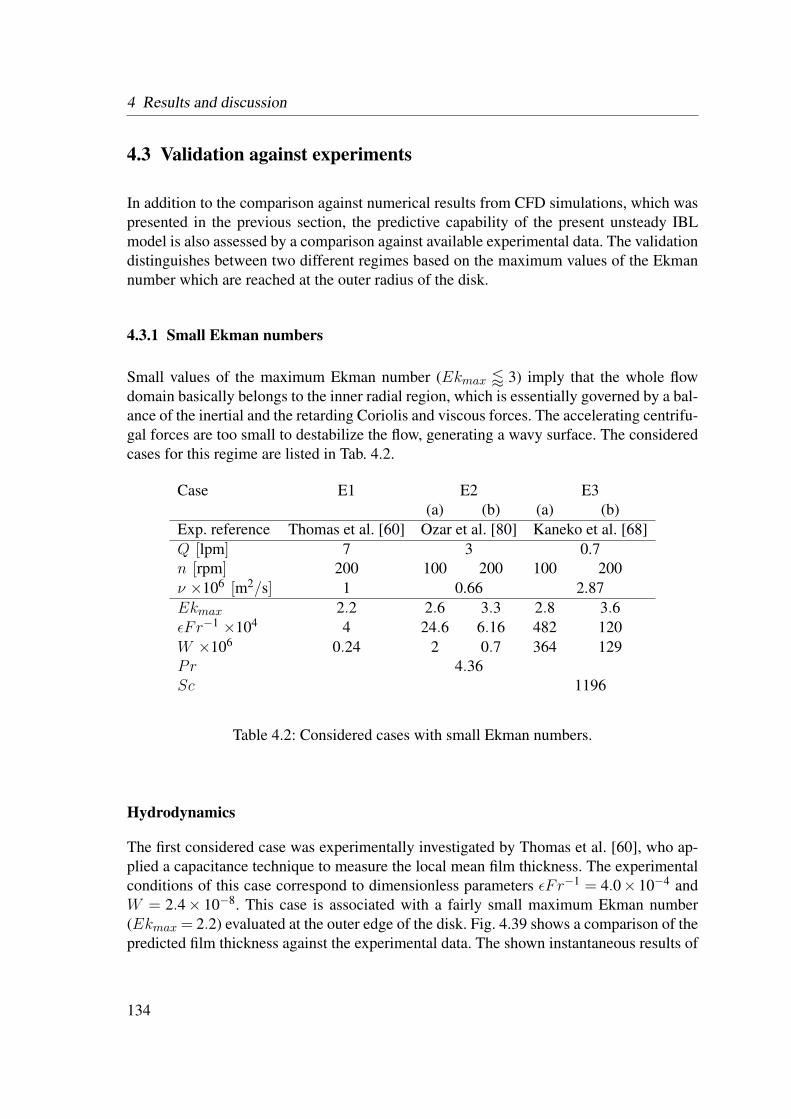
4 Results and discussion
4.3 Validation against experiments
In addition to the comparison against numerical results from CFD simulations, which waspresented in the previous section, the predictive capability of the present unsteady IBLmodel is also assessed by a comparison against available experimental data. The validationdistinguishes between two different regimes based on the maximum values of the Ekmannumber which are reached at the outer radius of the disk.
4.3.1 Small Ekman numbers
Small values of the maximum Ekman number (Ekmax / 3) imply that the whole flowdomain basically belongs to the inner radial region, which is essentially governed by a bal-ance of the inertial and the retarding Coriolis and viscous forces. The accelerating centrifu-gal forces are too small to destabilize the flow, generating a wavy surface. The consideredcases for this regime are listed in Tab. 4.2.
Case E1 E2 E3(a) (b) (a) (b)
Exp. reference Thomas et al. [60] Ozar et al. [80] Kaneko et al. [68]Q [lpm] 7 3 0.7n [rpm] 200 100 200 100 200ν ×106 [m2/s] 1 0.66 2.87Ekmax 2.2 2.6 3.3 2.8 3.6εFr−1 ×10⁴ 4 24.6 6.16 482 120W ×106 0.24 2 0.7 364 129Pr 4.36Sc 1196
Table 4.2: Considered cases with small Ekman numbers.
Hydrodynamics
The first considered case was experimentally investigated by Thomas et al. [60], who ap-plied a capacitance technique to measure the local mean film thickness. The experimentalconditions of this case correspond to dimensionless parameters εFr−1 = 4.0× 10⁻⁴ andW = 2.4× 10⁻⁸. This case is associated with a fairly small maximum Ekman number(Ekmax = 2.2) evaluated at the outer edge of the disk. Fig. 4.39 shows a comparison of thepredicted film thickness against the experimental data. The shown instantaneous results of
134
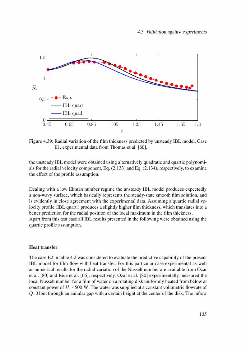
4.3 Validation against experiments
IBL quad.
IBL quart.
Exp.
〈δ〉
r
0.45 0.65 0.85 1.05 1.25 1.45 1.65 1.80
0.5
1
1.5
Figure 4.39: Radial variation of the film thickness predicted by unsteady IBL model. CaseE1, experimental data from Thomas et al. [60].
the unsteady IBL model were obtained using alternatively quadratic and quartic polynomi-als for the radial velocity component, Eq. (2.133) and Eq. (2.134), respectively, to examinethe effect of the profile assumption.
Dealing with a low Ekman number regime the unsteady IBL model produces expectedlya non-wavy surface, which basically represents the steady-state smooth film solution, andis evidently in close agreement with the experimental data. Assuming a quartic radial ve-locity profile (IBL quart.) produces a slightly higher film thickness, which translates into abetter prediction for the radial position of the local maximum in the film thickness.Apart from this test case all IBL results presented in the following were obtained using thequartic profile assumption.
Heat transfer
The case E2 in table 4.2 was considered to evaluate the predictive capability of the presentIBL model for film flow with heat transfer. For this particular case experimental as wellas numerical results for the radial variation of the Nusselt number are available from Ozaret al. [80] and Rice et al. [66], respectively. Ozar et al. [80] experimentally measured thelocal Nusselt number for a film of water on a rotating disk uniformly heated from below atconstant power ofH=4500 W. The water was supplied at a constant volumetric flowrate ofQ=3 lpm through an annular gap with a certain height at the center of the disk. The inflow
135

4 Results and discussion
temperature of the water was Ti=40 C. Accordingly, the fluid properties used for the IBLcomputation were set to ν=0.658×10⁻⁶ m2/s, λ=0.629 W/(mK) and cp=4179 J/(kgK).Given the uniformly heated area in the experiments the constant heat flux imposed at thewall is simply obtained as
qw =H
π(r2D− r2
i ). (4.13)
As suggested by Ozar et al. [80], the constant wall heat flux is also used in the definitionof the local Nusselt number written as
Nu=qwri
λ(Tw−Ti). (4.14)
According to this definition, the Nusselt number varies only dependent of the local walltemperature Tw. The comparison against the IBL predictions considers the experimen-tal and computational results obtained for two different rotation speeds, n=100 rpm andn=200 rpm. Based on the aforementioned flow rate and material properties the dimension-less parameters read εFr−1 = 24.6×10⁻⁴, W = 1.9×10⁻⁶, and Pr = 4.36, for the caseE2(a), and εFr−1 = 6.16× 10⁻⁴, W = 7× 10⁻⁷, and Pr = 4.36, for the case E2(b). Forboth considered cases the maximum Ekman number is again fairly small (Ekmax ≤ 3.3),and the unsteady IBL model consistently produced non-wavy smooth film solutions.
The radial variation of the Nusselt number, defined in Eq. (4.14), obtained for the rota-tional speeds n=100 and 200 rpm are shown in Figs. 4.40(a) and (b) respectively. In bothcases the predictions of the IBL model agree evidently very well with the experimentallyobtained results in the whole flow region covered by the measurements. It is interesting tonote that the observed overall agreement is even better than for the numerical results ofRice et al. [66], which show notable deviations at small radii.
Species mass transfer
As discussed in Sec. 2.4.2, the wet chemical etching of silicon using an etchant, whichbasically consists of nitric acid, is associated with large values of the Damköhler num-ber and very fast chemistry. Thus, the etching process is mainly controlled by the masstransfer of the HNO3 molecules towards the solid surface. In this limit of very largeDamköhler numbers the etching rate is therefore proportional to the local Sherwood num-ber, see Eq. (2.232).Fig. 4.41 shows a comparison of the IBL predictions for the etching rate obtained fromEq. (2.232) against experimental data from Kaneko et al. [68]. The liquid etchant was sup-plied at a constant volumetric flowrate of Q =0.67 lpm through an impinging jet emerg-ing from a nozzle with a diameter dn =6.5 mm. Two rotational speeds, n=100 rpm and
136
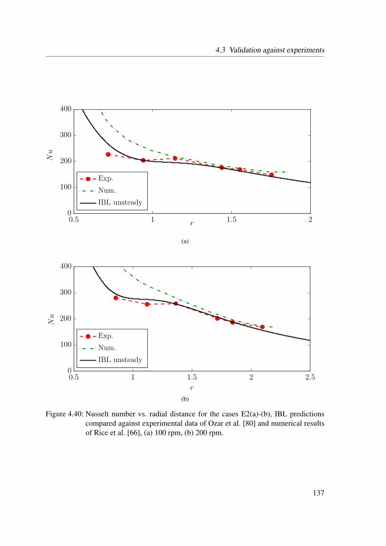
4.3 Validation against experiments
IBL unsteady
Num.
Exp.
Nu
r0.5 1 1.5 20
100
200
300
400
(a)
IBL unsteady
Num.
Exp.
Nu
r
0.5 1 1.5 2 2.50
100
200
300
400
(b)
Figure 4.40: Nusselt number vs. radial distance for the cases E2(a)-(b), IBL predictionscompared against experimental data of Ozar et al. [80] and numerical resultsof Rice et al. [66], (a) 100 rpm, (b) 200 rpm.
137
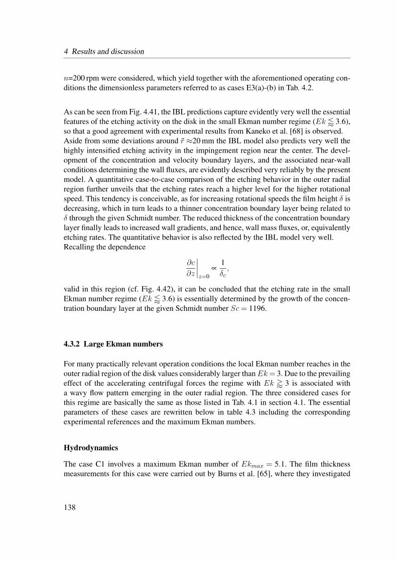
4 Results and discussion
n=200 rpm were considered, which yield together with the aforementioned operating con-ditions the dimensionless parameters referred to as cases E3(a)-(b) in Tab. 4.2.
As can be seen from Fig. 4.41, the IBL predictions capture evidently very well the essentialfeatures of the etching activity on the disk in the small Ekman number regime (Ek / 3.6),so that a good agreement with experimental results from Kaneko et al. [68] is observed.Aside from some deviations around r ≈20 mm the IBL model also predicts very well thehighly intensified etching activity in the impingement region near the center. The devel-opment of the concentration and velocity boundary layers, and the associated near-wallconditions determining the wall fluxes, are evidently described very reliably by the presentmodel. A quantitative case-to-case comparison of the etching behavior in the outer radialregion further unveils that the etching rates reach a higher level for the higher rotationalspeed. This tendency is conceivable, as for increasing rotational speeds the film height δ isdecreasing, which in turn leads to a thinner concentration boundary layer being related toδ through the given Schmidt number. The reduced thickness of the concentration boundarylayer finally leads to increased wall gradients, and hence, wall mass fluxes, or, equivalentlyetching rates. The quantitative behavior is also reflected by the IBL model very well.Recalling the dependence
∂c
∂z
∣∣∣∣z=0
∝1δc,
valid in this region (cf. Fig. 4.42), it can be concluded that the etching rate in the smallEkman number regime (Ek / 3.6) is essentially determined by the growth of the concen-tration boundary layer at the given Schmidt number Sc= 1196.
4.3.2 Large Ekman numbers
For many practically relevant operation conditions the local Ekman number reaches in theouter radial region of the disk values considerably larger thanEk= 3. Due to the prevailingeffect of the accelerating centrifugal forces the regime with Ek ' 3 is associated witha wavy flow pattern emerging in the outer radial region. The three considered cases forthis regime are basically the same as those listed in Tab. 4.1 in section 4.1. The essentialparameters of these cases are rewritten below in table 4.3 including the correspondingexperimental references and the maximum Ekman numbers.
Hydrodynamics
The case C1 involves a maximum Ekman number of Ekmax = 5.1. The film thicknessmeasurements for this case were carried out by Burns et al. [65], where they investigated
138

4.3 Validation against experiments
Exp.
IBL unsteady
R[µm/s]
r [mm]
0 10 20 30 40 50 60 70 800
0.1
0.2
0.3
0.4
0.5
0.6
0.7
(a)
Exp.
IBL unsteady
R[µm/s]
r [mm]
0 10 20 30 40 50 60 70 800
0.1
0.2
0.3
0.4
0.5
0.6
0.7
(b)
Figure 4.41: Etching rate vs. radial distance for the cases E3(a)-(b), IBL predictions com-pared against experimental data of Kaneko et al. [68], (a) 100 rpm, (b) 200rpm.
139

4 Results and discussion
c
δc
δ
〈δ〉,〈c〉
r0 0.5 1 1.5 2 2.5 30
0.5
1
1.5
Figure 4.42: IBL results for the radial variation of the film thickness, the thickness of theconcentration boundary layer, and the depth-averaged species mass fractionfor the case E3(b) with n=200 rpm.
a setup with a volumetric flowrate of Q=1.8 lpm, a rotational speed of n=401 rpm and aliquid with viscosity ν=1.3×10⁻⁶ m2/s.
Fig. 4.43 shows the time-averaged profiles of the film thickness predicted by the unsteadyIBL model together with the time-averaged profiles obtained from an axisymmetric CFDsimulation, and the experimental data of Burns et al. [65]. In the radially inner smoothregion, associated with r < 2 and Ek < 3, the IBL predictions again capture very wellthe height and the radial position of the local maximum of the film thickness and show asatisfactory overall agreement with the experimental as well as the numerical results.
Case C1 C2 C3Exp. reference Burns et al. [65] Staudegger [82] Staudegger et al. [85]Q [lpm] 1.8 1 1.25n [rpm] 401 500 500ν ×106 [m2/s] 1.3 1 2.87Ekmax 5.1 4.3 5.3εFr−1 ×10⁴ 5 4.5 10.3W ×106 0.19 3 9.35Pr 7Sc 1196
Table 4.3: Considered cases with large Ekman numbers.
140
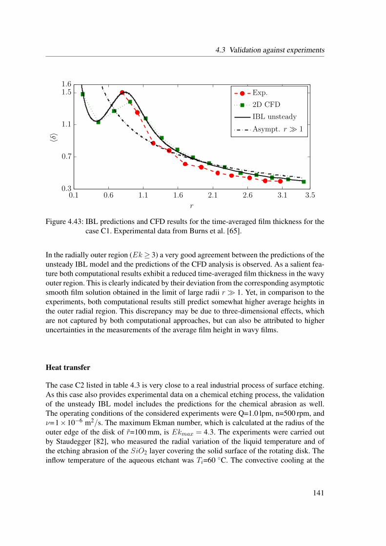
4.3 Validation against experiments
Asympt. r ≫ 1
IBL unsteady
2D CFD
Exp.
〈δ〉
r
0.1 0.6 1.1 1.6 2.1 2.6 3.1 3.50.3
0.7
1.1
1.51.6
Figure 4.43: IBL predictions and CFD results for the time-averaged film thickness for thecase C1. Experimental data from Burns et al. [65].
In the radially outer region (Ek≥ 3) a very good agreement between the predictions of theunsteady IBL model and the predictions of the CFD analysis is observed. As a salient fea-ture both computational results exhibit a reduced time-averaged film thickness in the wavyouter region. This is clearly indicated by their deviation from the corresponding asymptoticsmooth film solution obtained in the limit of large radii r 1. Yet, in comparison to theexperiments, both computational results still predict somewhat higher average heights inthe outer radial region. This discrepancy may be due to three-dimensional effects, whichare not captured by both computational approaches, but can also be attributed to higheruncertainties in the measurements of the average film height in wavy films.
Heat transfer
The case C2 listed in table 4.3 is very close to a real industrial process of surface etching.As this case also provides experimental data on a chemical etching process, the validationof the unsteady IBL model includes the predictions for the chemical abrasion as well.The operating conditions of the considered experiments were Q=1.0 lpm, n=500 rpm, andν=1×10⁻⁶ m2/s. The maximum Ekman number, which is calculated at the radius of theouter edge of the disk of r=100 mm, is Ekmax = 4.3. The experiments were carried outby Staudegger [82], who measured the radial variation of the liquid temperature and ofthe etching abrasion of the SiO2 layer covering the solid surface of the rotating disk. Theinflow temperature of the aqueous etchant was Ti=60 C. The convective cooling at the
141
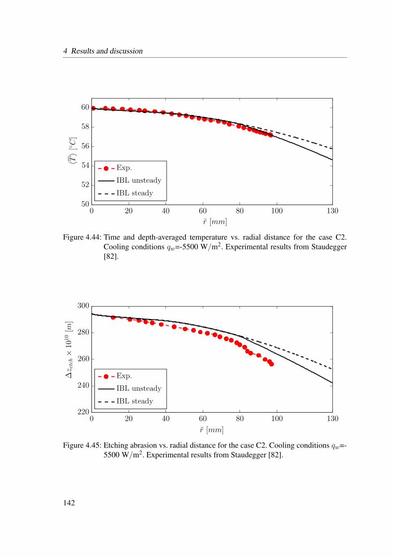
4 Results and discussion
IBL steady
IBL unsteady
Exp.
〈T〉[
C]
r [mm]
0 20 40 60 80 100 13050
52
54
56
58
60
Figure 4.44: Time and depth-averaged temperature vs. radial distance for the case C2.Cooling conditions qw=-5500 W/m2. Experimental results from Staudegger[82].
IBL steady
IBL unsteady
Exp.∆z e
tch×
1010
[m]
r [mm]
0 20 40 60 80 100 130220
240
260
280
300
Figure 4.45: Etching abrasion vs. radial distance for the case C2. Cooling conditions qw=-5500 W/m2. Experimental results from Staudegger [82].
142

4.3 Validation against experiments
downside of the disk, which was realized in the experiments with a stream of nitrogen ascoolant medium, was prescribed in terms of a constant wall heat flux qw=-5500 W/m2 inthe computation.As seen from Fig. 4.44, the time-averaged predictions from the IBL approximation forthe depth-averaged temperature agree very well with the experimentally obtained data. Acomparison against the corresponding steady-state smooth film solution underlines againthe importance of capturing the unsteady waviness in the outer radial region. This aspectis also clearly reflected by the predictions for the etching abrasion shown in Fig. 4.45.Assuming a mainly temperature dependent model for the chemistry, as it is applicable inthe here considered limit of very small Damköhler numbers (cf. Sec. 2.4.1), the improvedpredictions for the temperature translate directly into better predictions for the etchingresults.
Species mass transfer
The here considered case is referred to as C3 in Tab. 4.3. In contrast to the reaction con-trolled case C2, the case C3 involves a diffusion controlled chemistry assuming very fastetching reactions. In this limit of high Damköhler number the etching rate is basically de-termined by the species mass flux of the etchant into the wall as given by Eq. (2.232). Assuch the etching rate is equivalent to the Sherwood number.
In Fig. 4.46 the computed time-averaged etching rate is compared against experimentaldata obtained by Staudegger et al. [85]. In the radially inner smooth region, associatedwith r / 2 and Ek / 3, the IBL predictions again capture very well the experimentallyobserved etching rates. Dealing with high Schmidt number flow the thickness of the con-centration boundary layer remains smaller than the film thickness in this region, (compare,e.g. Fig. 4.29, for the case C3 with Sc = 1196), so that the radial variation of the etch-ing rate is essentially determined by the growth of the concentration boundary layer. Theregion, where good agreement with the experiments is observed, is evidently restricted tothe inner and middle region associated with Ek / 4, as can be seen from Fig. 4.46(b).In the outer region, the unsteady IBL solution predicts a significant decrease of the localtime-averaged Sherwood number, which translates into a decrease of the etching rate. Thispeculiar feature is evidently not supported by the experiments, as seen from the significantdeviations in the radially outer region.
A very similar tendency is seen in the predictions for the etching rates obtained for awide range of operating conditions, as shown in Figs. 4.47-4.48. While generally verygood agreement is found in the radially inner and middle regions, the unsteady IBL modelalways underpredicts the experimentally observed rates in the radially outer region associ-ated withEk' 4. As seen from Figs. 4.49(a)-(b), which exemplarily depict the steady-state
143
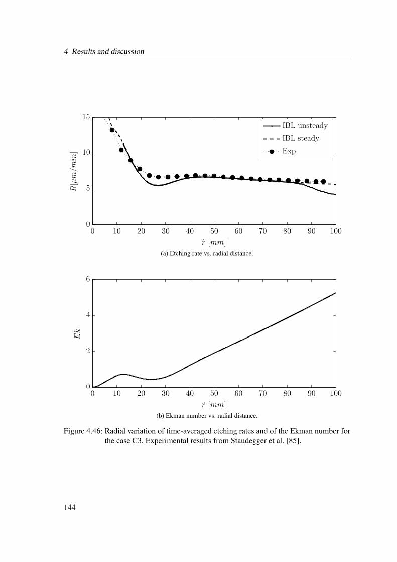
4 Results and discussion
Exp.
IBL steady
IBL unsteady
R[µm/m
in]
r [mm]
0 10 20 30 40 50 60 70 80 90 1000
5
10
15
(a) Etching rate vs. radial distance.
Ek
r [mm]
0 10 20 30 40 50 60 70 80 90 1000
2
4
6
(b) Ekman number vs. radial distance.
Figure 4.46: Radial variation of time-averaged etching rates and of the Ekman number forthe case C3. Experimental results from Staudegger et al. [85].
144
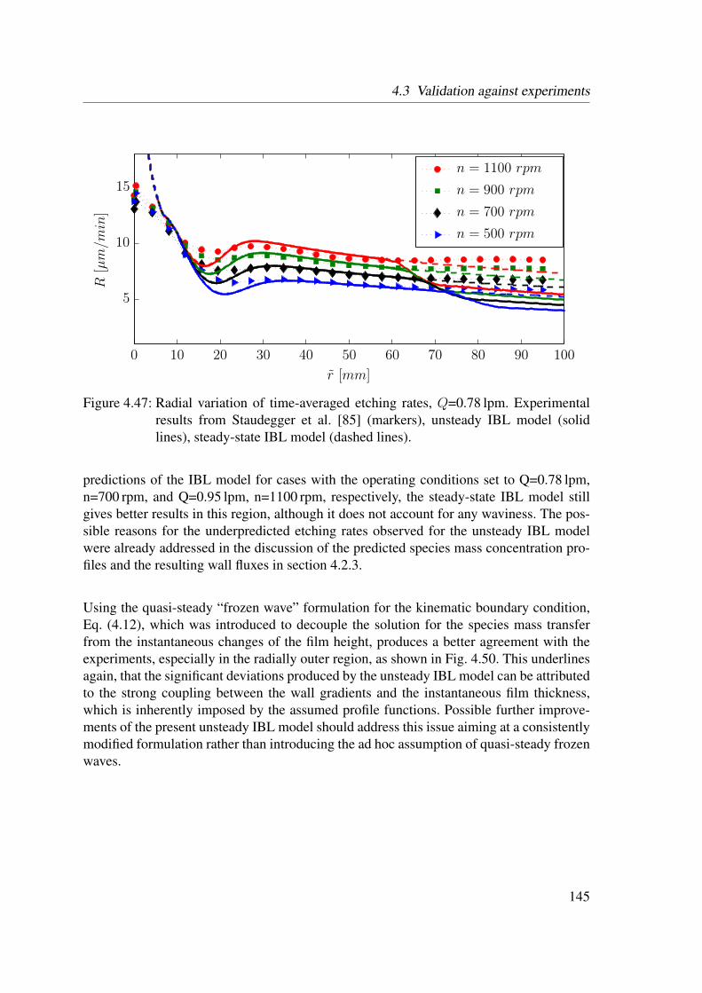
4.3 Validation against experiments
n = 500 rpm
n = 700 rpm
n = 900 rpm
n = 1100 rpm
R[µm/m
in]
r [mm]
0 10 20 30 40 50 60 70 80 90 100
5
10
15
Figure 4.47: Radial variation of time-averaged etching rates, Q=0.78 lpm. Experimentalresults from Staudegger et al. [85] (markers), unsteady IBL model (solidlines), steady-state IBL model (dashed lines).
predictions of the IBL model for cases with the operating conditions set to Q=0.78 lpm,n=700 rpm, and Q=0.95 lpm, n=1100 rpm, respectively, the steady-state IBL model stillgives better results in this region, although it does not account for any waviness. The pos-sible reasons for the underpredicted etching rates observed for the unsteady IBL modelwere already addressed in the discussion of the predicted species mass concentration pro-files and the resulting wall fluxes in section 4.2.3.
Using the quasi-steady “frozen wave” formulation for the kinematic boundary condition,Eq. (4.12), which was introduced to decouple the solution for the species mass transferfrom the instantaneous changes of the film height, produces a better agreement with theexperiments, especially in the radially outer region, as shown in Fig. 4.50. This underlinesagain, that the significant deviations produced by the unsteady IBL model can be attributedto the strong coupling between the wall gradients and the instantaneous film thickness,which is inherently imposed by the assumed profile functions. Possible further improve-ments of the present unsteady IBL model should address this issue aiming at a consistentlymodified formulation rather than introducing the ad hoc assumption of quasi-steady frozenwaves.
145
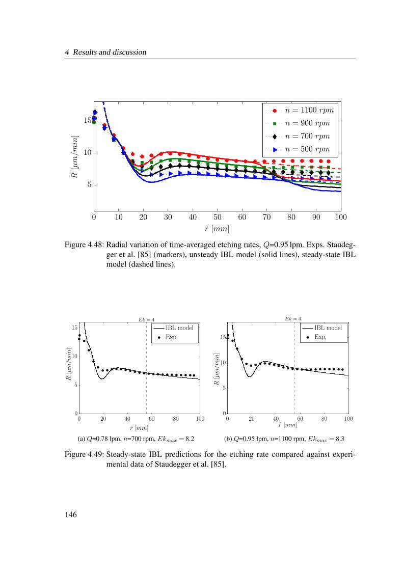
4 Results and discussion
n = 500 rpm
n = 700 rpm
n = 900 rpm
n = 1100 rpm
R[µm/m
in]
r [mm]
0 10 20 30 40 50 60 70 80 90 100
5
10
15
Figure 4.48: Radial variation of time-averaged etching rates, Q=0.95 lpm. Exps. Staudeg-ger et al. [85] (markers), unsteady IBL model (solid lines), steady-state IBLmodel (dashed lines).
Ek = 4
Exp.
IBL model
R[µm/m
in]
r [mm]
0 20 40 60 80 1000
5
10
15
(a) Q=0.78 lpm, n=700 rpm, Ekmax = 8.2
Ek = 4
Exp.
IBL model
R[µm/m
in]
r [mm]0 20 40 60 80 1000
5
10
15
(b) Q=0.95 lpm, n=1100 rpm, Ekmax = 8.3
Figure 4.49: Steady-state IBL predictions for the etching rate compared against experi-mental data of Staudegger et al. [85].
146

4.3 Validation against experiments
steady IBL
unsteady IBL, quasi-steady kin. b.c.
Exp.
R[µm/m
in]
r [mm]
0 10 20 30 40 50 60 70 80 90 1000
5
10
15
20
Figure 4.50: Solution of unsteady IBL model using quasi-steady “frozen-wave“ kinematicboundary condition for Q=0.78 lpm, n=1100 rpm.
147


5 CONCLUSIONS AND RECOMMENDATIONS FOR FURTHERWORK
The present work investigated computationally the hydrodynamic, heat and species masstransfer of thin liquid film flow on rotating disks using an unsteady integral boundary layer(IBL) model. In the framework of this model the governing unsteady boundary layer typeequations are averaged over the film height, assuming polynomial ansatz functions forthe profiles of the individual velocity components, the dimensionless temperature, and thespecies mass fraction. Aside from the analysis of the salient steady-state features met inthe smooth film regime the focus was particularly put on the effect of the unsteady surfacewaves on the momentum, heat and species mass transfer.
In the inner radial region, r / 2, associated with small Ekman numbers, Ek / 3, whereCoriolis forces exert a stabilizing influence, the predictions of the present unsteady IBLmodel consistently exhibit a non-wavy smooth surface. It can be inferred that the smallEkman number regime allows for the computationally simpler steady-state IBL model,which can describe only smooth film flow. The results which were obtained with the IBLmodel in this region for the radial variation of the film thickness, the Nusselt number, andthe Sherwood number are in very good agreement with corresponding experimental data.In the cases with larger values of the local Ekman number, Ek ≥ 3, the unsteady com-putations reproduced very well the formation and further propagation of surface wavestriggered by the destabilizing influence of the radially increasing centrifugal forces. Acomparison of the time-averaged results of the unsteady IBL model against correspond-ing steady-state smooth film solutions unveiled a reduced averaged film thickness as oneof the major effects of the waviness. As for the heat transfer the waviness led to an in-creased/decreased film temperature in the heating/cooling wall heat flux cases. The reasonfor these most salient effects, which are also observed in experiments, could be identifiedby a close analysis of the evolution of the instantaneous flow and thermal quantities. Inthe wavy region most of the liquid volume is transported by fast moving surface waves,whose passage is generally intermittent with comparatively longer periods with very thinliquid coverage, which effectively reduces the average film thickness. The thin liquid lay-ers occurring between the surface waves are more easily heated-up/cooled-down by theheating/cooling wall heat flux, which explains the increased/decreased film temperaturesin the wavy regime.The practical importance of accounting appropriately for the effects of surface waviness ishighlighted by including a wet chemical etching model valid for low Damköhler numbers.
149

5 Conclusions and recommendations for further work
Applying the so extended unsteady IBL model to a technically relevant test case yieldeda markedly improved agreement with available experimental data as compared to a corre-sponding steady-state smooth film solution.
The high level of description demonstrated by the present unsteady IBL model for thehydrodynamics and the heat transfer in the unsteady wavy regime was not observed forthe species mass transfer. In contrast to experiments and CFD simulations the IBL resultsalways exhibited a rapid decrease in the wall mass flux at the onset of waviness.In a detailed analysis of the velocity and mass fraction profiles it was found that the ob-served deficits of the present unsteady IBL model can be mainly attributed to some in-herent limitations of the assumed profile functions. In particular, large discrepancies wereobserved for the w-profile, which is implicitly determined by the polynomials assumedfor the radial and azimuthal components of the velocity. In addition the assumed profilefunctions scale with the film height. This inherently imposes a strong coupling betweenthe instantaneous local variations in the height of the liquid and the near wall conditionsinside the concentration boundary layer, which finally produces an exaggeratedly strongthickening of the concentration boundary layer when the surface becomes wavy. This de-scriptive limitation is specially relevant for the high Schmidt number cases considered inthis work (Sc ≈ 1200). The very thin concentration boundary layers are expected to beless influenced by the flow condition at the liquid surface, which speaks against the strongcoupling incorporated by the assumed profile functions.
Summing up, it can be stated that the present unsteady IBL method was shown to capturethe essential hydrodynamic and thermal features of the wavy thin film flow on a spinningdisk at a high level of description. Major restrictions only become evident when consider-ing species mass transfer in a binary mixture for the particular case with very large Schmidtnumbers. Aside from this limitation, the present unsteady IBL approximation has provenas a reliable and computationally efficient approach to investigate wavy flow on rotatingdisks, including heat and mass transfer. As such the present concept offers a great potentialas computational design and optimization tool for spinning disk devices, which are widelyused for various wet processing applications.
Recommendations for further work
Relevant topics for further studies are an improvement of the present IBL model by uti-lizing the weighted residual integral boundary layer (WRIBL) approach (see, e.g. Ruyer-Quil & Manneville [28, 29], Trevelyan et al. [112]) instead of simple polynomial profileassumptions, as the major limitations of the present model were found to be related tothe polynomial ansatz functions, which are required for the depth-averaging. In the frame-work of the WRIBL approach it should be possible to model the recirculation zones, which
150

appear inside solitary waves. An appropriate modeling of these recirculation zones is ex-pected to improve also the predictions for heat and species mass transfer.
Furthermore the present IBL model should be extended to model three-dimensional flow(2D IBL model, see e.g. appendix 4), as the assumption of axisymmetric conditions is onlyvalid in a very restricted range of operating conditions. A three-dimensional model wouldadditionally offer the possibility to model cases with off-center impingement, which arehighly relevant for various industrial applications. In this framework also a proper ansatzfor the description of the formation of dry spots will have to be included.It may be also interesting to include edge effects, as the fluid flow over disk edge typicallyresults in the formation of a liquid rim due to the increased pressure caused by the surfacetension.
A further validation of the IBL predictions and the CFD results against more comprehen-sive experimental data, including experimental data describing instantaneous flow features,would be desirable.
151


Appendices
153

1 Divergence (Gauss’s) theorem
1 Divergence (Gauss’s) theorem
Gauss’s theorem relates the volume integral of the divergence of a vector, ∇ · ~F , over thevolume V , with the surface integral over the boundary of this volume, ∂V ≡ S, by
∫
V
(∇ · ~F
)dV =
∫
S
~F ·d~S. (1)
Physically this can be interpreted as conservation law, which states that the net flux acrossthe boundary S equals the source rate inside V .
2 Relations and profile parameters for the IBL model
2.1 Quadratic approximation
u=1δ
δ∫
0
u(z)dz =
ζ∫
0
uδ(2ζ− ζ2)dζ = 2
3uδ (2)
v =1δ
δ∫
0
v(z)dz =
ζ∫
0
vδ
(85ζ− 4
5ζ3 +
15ζ4)dζ =
1625vδ. (3)
w =1δ
δ∫
0
w(z)dz =
ζ∫
0
wδ
[ζ2(
32−aw(r)
)+ ζ3
(aw(r)−
12
)]dζ
= wδ
(38− aw(r)
12
). (4)
ka =
∫ ζ0 u
2δ
(2ζ− ζ2)2
dζ
u2 =65
(5)
155

kb =
∫ ζ0 uδ
(2ζ− ζ2)vδ
(85ζ− 4
5ζ3 + 1
5ζ4)dζ
uv=
1714
(6)
kc =
∫ ζ0 v
2δ
(85ζ− 4
5ζ3 + 1
5ζ4)2
dζ
v2 =155126
(7)
∂u
∂z
∣∣∣∣z=0
= 3u
δ(8)
∂v
∂z
∣∣∣∣z=0
=52v
δ(9)
2.2 Quartic approximation
u=1δ
δ∫
0
u(z)dz =1625uδ+
κδ2
75(10)
uδ =2516u− κδ
2
48(11)
v =1δ
δ∫
0
v(z)dz =1625uδ+
κ2δ2
75(12)
vδ =2516u− κδ
2
48. (13)
∂u
∂z
∣∣∣∣z=0
=52u
δ+
16κδ (14)
∂v
∂z
∣∣∣∣z=0
=52v
δ+
16κ2δ (15)
156
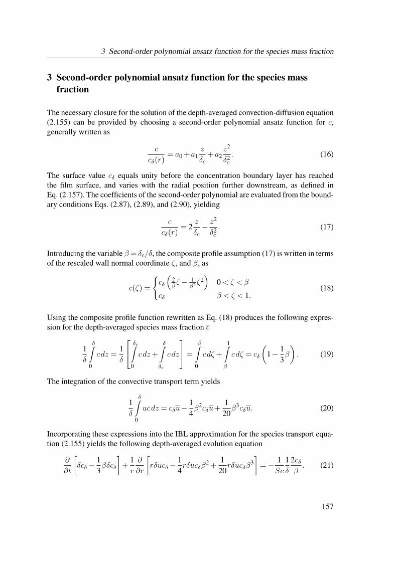
3 Second-order polynomial ansatz function for the species mass fraction
3 Second-order polynomial ansatz function for the species massfraction
The necessary closure for the solution of the depth-averaged convection-diffusion equation(2.155) can be provided by choosing a second-order polynomial ansatz function for c,generally written as
c
cδ(r)= a0 +a1
z
δc+a2
z2
δ2c. (16)
The surface value cδ equals unity before the concentration boundary layer has reachedthe film surface, and varies with the radial position further downstream, as defined inEq. (2.157). The coefficients of the second-order polynomial are evaluated from the bound-ary conditions Eqs. (2.87), (2.89), and (2.90), yielding
c
cδ(r)= 2
z
δc− z
2
δ2c. (17)
Introducing the variable β= δc/δ, the composite profile assumption (17) is written in termsof the rescaled wall normal coordinate ζ , and β, as
c(ζ) =
cδ
(2β ζ− 1
β2 ζ2)
0 < ζ < β
cδ β < ζ < 1.(18)
Using the composite profile function rewritten as Eq. (18) produces the following expres-sion for the depth-averaged species mass fraction c
1δ
δ∫
0
cdz =1δ
δc∫
0
cdz+
δ∫
δc
cdz
=
β∫
0
cdζ+
1∫
β
cdζ = cδ
(1− 1
3β
). (19)
The integration of the convective transport term yields
1δ
δ∫
0
ucdz = cδu−14β2cδu+
120β3cδu. (20)
Incorporating these expressions into the IBL approximation for the species transport equa-tion (2.155) yields the following depth-averaged evolution equation
∂
∂t
[δcδ−
13βδcδ
]+
1r
∂
∂r
[rδucδ−
14rδucδβ
2 +120rδucδβ
3]=− 1
Sc
1δ
2cδβ. (21)
157
Reformulating Eq. (21) in terms of the total directional derivatives, considering addition-ally the flow to be axisymmetric, yields
(6√ω
cδ− 2ωcδ
)[∂cδ∂t
+15ω−3ω3/2−60
20√ω−60
u∂cδ∂r
]−
[∂ω
∂t+
(32√ω− 9
20ω
)u∂ω
∂r
]=
− 12Sc
1δ2 −
1δ
∂δ
∂t
(−2ω+
32ω3/2− 3
10ω2). (22)
Again Eq. (22) can be separately solved for ω and cδ as their total directional derivativesbecome alternately zero.
Steady-state species mass transfer
Utilizing the second-order polynomial ansatz function given by Eq. (17), the depth-averagedconvection-diffusion equation for the steady-state species mass transfer reduces to
β < 1, cδ = 1 :dδcdr
= βdδ
dr+
r
Sc
(360
30β2−9β3
),
β = 1, cδ < 1 :dcδdr
=−152rcδδSc
.
(23)
Considering the steady-state approximation for the film thickness to be given by δ= r−2/3,an asymptotic solution in the limit of large radii for the species mass fraction at the freesurface is obtained as
β = 1, cδ < 1 : sδ(r) = exp[− 45
16Sc
(r8/3− r8/3
c
)]. (24)
158
4 IBL approximation for three-dimensional film flow
4 IBL approximation for three-dimensional film flow
In the limit of the thin film approximation the governing equations for the three-dimensionalflow on a spinning disk are given by Eqs. (2.63)-(2.68). The kinematic boundary conditionreads
z = δ : w =∂δ
∂t+u
∂δ
∂r+v
r
∂δ
∂φ, (25)
and the stress-free conditions on the free surface at z = δ are given by
τrz =∂u
∂z= 0, (26)
τφz =∂v
∂z= 0, (27)
0 =−p−W(
1r
∂
∂r
(r∂δ
∂r
)+
1r2∂2δ
∂φ2
). (28)
The depth-averaged continuity equation for the three-dimensional flow is obtained as
∂δ
∂t+
1r
∂
∂r[ruδ]+
1r
∂
∂φ[vδ] = 0. (29)
Introducing an improved profile assumption for the azimuthal component of the velocityas (see, e.g., Kim & Kim [75])
v(ζ) = vδ
(85ζ− 4
5ζ3 +
15ζ4)+κ2δ
2
5ζ (1− ζ)2
(1− ζ
2
). (30)
the depth-averaged momentum equations in radial and azimuthal direction read
∂ (δu)
∂t+kar
∂
∂r
(rδu2)+ kb
r
∂
∂φ(u vδ)− kcδv
2
r=
β1δ
(r− ∂P
∂r
)+2δv−β2
u
δ, (31)
and
∂ (δv)
∂t+kbr
∂
∂r(rδu v)+
kcr
∂
∂φ
(v2δ)+kbδu v
r=
− 56δ
r
∂P
∂φ−2δu− 5
2v
δ, (32)
159
respectively.Depth averaging of the convection-diffusion equation for the transport of a general passivescalar quantity, denoted by s, yields
∂
∂t[δΦ]+
1r
∂
∂r[rδΨ ]+
1r
∂
∂φ[δΠ] =− 1
K
∂s
∂z
∣∣∣∣z=0
. (33)
Here K is the characteristic dimensionless variable for the transport of the passive scalar,e.g. the Schmidt number in case of species transport (s ≡ c). The capital Greek letterssupersede the integrals
Φ=1δ
δ∫
0
sdz, (34)
Ψ =1δ
δ∫
0
usdz, (35)
and
Π =1δ
δ∫
0
vsdz. (36)
Assuming a Dirichlet boundary condition for the passive scalar
s|z=0 = 0, (37)
the depth-averaged transport equation is obtained as
∂
∂t
[δsδ−
38βδsδ
]+
1r
∂
∂r
[rδusδ−
310rδusδβ
2 +1
16rδusδβ
3]
+1r
∂
∂φ
[δvsδ−
14δvsδβ
2 +3
112δvsδβ
4− 1256
δvsδβ5]=− 1
K
1δ
3sδ2β
. (38)
Therein a third-order polynomial ansatz function was chosen as closure relation. Reformu-lating Eq. (38) in terms of ω, utilizing the depth-averaged continuity equation, Eq. (29) to
160
4 IBL approximation for three-dimensional film flow
substitute ∂δ/∂t, yields(
16√ω
3sδ− 2ωsδ
)
[∂sδ∂t
+80−24ω+5ω3/2
80−30√ω
u∂sδ∂r
+448ω−48ω2 +7ω5/2−1792
672√ω−1792
v
r
∂sδ∂φ
]
−[∂ω
∂t+
(85√ω− 1
2ω
)u∂ω
∂r+
(43√ω− 2
7ω3/2 +
596ω2)v
r
∂ω
∂φ
]=
− 8K
1δ2 −
1δ
1r
∂
∂r(ruδ)
(2ω− 8
5ω3/2 +
13ω2)
− 1δ
1r
∂
∂φ(vδ)
(2ω− 4
3ω3/2 +
17ω5/2− 1
48ω7/2
). (39)
0 δ a chemD diff etch imax w nLG 〈〉 () ( ) ~() ∇ ()TM(a,b,c)H(x)Γ (a)γ(a,x)D1,2awka,b,c k C p r φ z u v w t g M b1,2
δ δr,φ δT δc
α ϕ γ u0 w0 p0 t0 Sh
161

BIBLIOGRAPHY
[1] C. Park and T. Nosoko, “Three-dimensional wave dynamics on a falling film andassociated mass transfer,” AIChE Journal, vol. 49, no. 11, pp. 2715–2727, 2003.
[2] D. Prieling, H. Steiner, W. Meile, and G. Brenn, “High-speed camera recordings ofwavy liquid films on spinning disks,” tech. rep., Institute of Fluid Mechanics andHeat Transfer, Graz University of Technology, 2010.
[3] H.-C. Chang and E. Demekhin, Complex wave dynamics on thin films. ElsevierScience, 2002.
[4] S. Kalliadasis, C. Ruyer-Quil, B. Scheid, and M. Velarde, Falling liquid films.Springer Verlag, 2011.
[5] A. Oron, S. Davis, and S. Bankoff, “Long-scale evolution of thin liquid films,” Re-views of Modern Physics, vol. 69, no. 3, pp. 931–980, 1997.
[6] R. Craster and O. Matar, “Dynamics and stability of thin liquid films,” Reviews ofModern Physics, vol. 81, no. 3, pp. 1131–1198, 2009.
[7] W. Nusselt, “Die Oberflächenkondensation des Wasserdampfes,” Zeitschrift desVereins Deutsche Ingenieure, vol. 60, pp. 541–546, 1916.
[8] P. Kapitza and S. Kapitza, “Wave flow of thin fluid layers of liquid,” Soviet Journalof Experimental and Theoretical Physics, vol. 19, pp. 105–120, 1949.
[9] T. Benjamin, “Wave formation in laminar flow down an inclined plane,” Journal ofFluid Mechanics, vol. 2, no. 6, pp. 554–573, 1957.
[10] C. Yih, “Stability of liquid flow down an inclined plane,” Physics of Fluids, vol. 6,no. 3, pp. 321–334, 1963.
[11] A. Binnie, “Experiments on the onset of wave formation on a film of water flowingdown a vertical plate,” Journal of Fluid Mechanics, vol. 2, no. 6, pp. 551–553, 1957.
[12] A. Binnie, “Instability in a slightly inclined water channel,” Journal of Fluid Me-chanics, vol. 5, no. 4, pp. 561–570, 1959.
[13] S. Tailby and S. Portalski, “The hydrodynamics of liquid films flowing on verticalsurface,” Transactions of the Institution of Chemical Engineers, vol. 38, pp. 324–330, 1960.
163

Bibliography
[14] S. Joo and S. Davis, “Instabilities of three-dimensional viscous falling films,” Jour-nal of Fluid Mechanics, vol. 242, no. 1, pp. 529–547, 1992.
[15] M. Cheng and H. Chang, “Competition between subharmonic and sideband sec-ondary instabilities on a falling film,” Physics of Fluids, vol. 7, no. 1, pp. 34–54,1995.
[16] D. Benney, “Long waves on liquid films,” Journal of Mathematical Physics, vol. 45,no. 2, pp. 150–155, 1966.
[17] H. Chang, “Travelling waves on fluid interfaces: Normal form analysis of thekuramoto-sivashinsky equation,” Physics of Fluids, vol. 29, no. 10, pp. 3142–3147,1986.
[18] T. Yang, “On traveling-wave solutions of the Kuramoto-Sivashinsky equation,”Physica D: Nonlinear Phenomena, vol. 110, no. 1, pp. 25–42, 1997.
[19] P. Kapitza, “Wave flow of thin viscous fluid layers,” Soviet Journal of Experimentaland Theoretical Physics, vol. 18, no. 1, pp. 3–28, 1948.
[20] V. Shkadov, “Wave modes in the gravity flow of a thin layer of a viscous fluid,” Izv.Akad. Nauk. SSSR, Mekh. Zhid. i Gaza, vol. 1, pp. 43–51, 1967.
[21] J. Wilkes and R. Nedderman, “The measurement of velocities in thin films of liq-uid,” Chemical Engineering Science, vol. 17, no. 3, pp. 177–187, 1962.
[22] S. S. Portalski, “Velocities in film flow of liquids on vertical plates,” Chemical En-gineering Science, vol. 19, no. 8, pp. 575–582, 1964.
[23] A. Bunov, E. Demekhin, and V. Shkadov, “On the non-uniqueness. of non-linearwave solutions in a viscous layer,” Journal of Applied Mathematics and Mechanics,vol. 48, no. 4, pp. 495–499, 1984.
[24] G. Sisoev and V. Shkadov, “On two-parametric manifold of the waves solutions ofequation for falling film of viscous liquid,” Doklady Physics, vol. 44, no. 7, pp. 454–459, 1999.
[25] G. Sisoev and V. Shkadov, “Dominant waves in a viscous liquid flowing in a thinsheet,” Doklady Physics, vol. 42, no. 12, pp. 683–686, 1997.
[26] G. Sisoev and V. Shkadov, “Development of dominating waves from small distur-bances in falling viscous-liquid films,” Fluid Dynamics, vol. 32, no. 6, pp. 794–792,1997.
[27] S. Alekseenko, V. Nakoriakov, B. Pokusaev, and T. Fukano, Wave flow of liquidfilms. Begell House, New York, 1994.
164
Bibliography
[28] C. Ruyer-Quil and P. Manneville, “Modeling film flows down inclined planes,”The European Physical Journal B-Condensed Matter and Complex Systems, vol. 6,no. 2, pp. 277–292, 1998.
[29] C. Ruyer-Quil and P. Manneville, “Improved modeling of flows down inclinedplanes,” The European Physical Journal B-Condensed Matter and Complex Sys-tems, vol. 15, no. 2, pp. 357–369, 2000.
[30] B. Scheid, C. Ruyer-Quil, and P. Manneville, “Wave patterns in film flows: mod-elling and three-dimensional waves,” Journal of Fluid Mechanics, vol. 562, no. 1,pp. 183–222, 2006.
[31] T. Salamon, R. Armstrong, and R. Brown, “Traveling waves on vertical films: Nu-merical analysis using the finite element method,” Physics of Fluids, vol. 6, no. 6,pp. 2202–2220, 1994.
[32] N. Malamataris, M. Vlachogiannis, and V. Bontozoglou, “Solitary waves on in-clined films: Flow structure and binary interactions,” Physics of Fluids, vol. 14,no. 3, pp. 1082–1094, 2002.
[33] J. Liu and J. Gollub, “Solitary wave dynamics of film flows,” Physics of Fluids,vol. 6, no. 5, pp. 1702–1712, 1994.
[34] J. Liu, J. Schneider, and J. Gollub, “Three-dimensional instabilities of film flows,”Physics of Fluids, vol. 7, no. 1, pp. 55–67, 1995.
[35] S. Alekseenko, V. Antipin, V. Guzanov, S. Kharlamov, and D. Markovich, “Three-dimensional solitary waves on falling liquid film at low Reynolds numbers,” Physicsof Fluids, vol. 17, no. 12, pp. 121704.1–121704.4, 2005.
[36] N. Malamataris and T. Papanastasiou, “Unsteady free surface flows on truncateddomains,” Industrial & Engineering Chemistry Research, vol. 30, no. 9, pp. 2211–2219, 1991.
[37] S. Jayanti and G. Hewitt, “Hydrodynamics and heat transfer of wavy thin film flow,”International Journal of Heat and Mass Transfer, vol. 40, no. 1, pp. 179–190, 1997.
[38] D. Gao, N. Morley, and V. Dhir, “Numerical simulation of wavy falling film flowusing VOF method,” Journal of Computational Physics, vol. 192, no. 2, pp. 624–642, 2003.
[39] P. Kapitza, Collected papers by P. L. Kapitza. New York: Macmillan, 1964.
[40] T. Nosoko, P. Yoshimura, T. Nagata, and K. Oyakawa, “Characteristics of two-dimensional waves on a falling liquid film,” Chemical Engineering Science, vol. 51,no. 5, pp. 725–732, 1996.
165
Bibliography
[41] S. Yih, “Modelling heat and mass transport in falling liquid films,” in Handbook ofHeat and Mass Transfer, vol. 2, ch. 5, pp. 111–210, 1986.
[42] C. Kirkbride, “Heat transfer by condensing vapors on. vertical tubes,” Transactionsof American Institute of Chemical Engineers, vol. 30, pp. 170–193, 1934.
[43] K. Chun and R. A. R.A. Seban, “Heat transfer to evaporating liquid films,” Journalof Heat Transfer, vol. 93, pp. 391–396, 1971.
[44] R. Hirshburg and L. Florschuetz, “Laminar wavy-film flow: Part I, hydrodynamicanalysis,” Journal of Heat Transfer, vol. 104, no. 3, pp. 452–458, 1982.
[45] R. Hirshburg and L. Florschuetz, “Laminar wavy-film flow: Part II, condensationand evaporation,” Journal of Heat Transfer, vol. 104, no. 3, pp. 459–464, 1982.
[46] A. Miyara, “Numerical analysis on heat transfer enhancement by waves on fallingliquid film,” Journal of Thermal Science, vol. 9, pp. 236–242, 2000.
[47] R. Emmert and R. Pigford, “Interfacial resistance-gas absorption in falling liquidfilm,” Chemical Engineering Progress, vol. 50, pp. 87–93, 1954.
[48] E. Ruckenstein and C. Berbente, “Mass transfer in wavy flow,” Chemical Engineer-ing Science, vol. 20, pp. 795–801, 1965.
[49] F. Wasden and A. Dukler, “A numerical study of mass transfer in free falling wavyfilms,” A.I.Ch.E. Journal, vol. 9, no. 36, pp. 1379–1390, 1990.
[50] G. Sisoev, O. Matar, and C. Lawrence, “Absorption of gas into a wavy falling film,”Chemical Engineering Science, vol. 60, no. 3, pp. 827–838, 2005.
[51] T. Hirose, Y. Mori, and Y. Sato, “Solid-liquid mass transfer in falling liquid films onsingle spheres,” Journal of Chemical Engineering of Japan, vol. 7, no. 1, pp. 19–24,1974.
[52] N. Brauner and D. Moalem-Maron, “Characteristics of inclined thin films, wavinessand the associated mass transfer,” International Journal of Heat and Mass Transfer,vol. 25, no. 1, pp. 99–110, 1982.
[53] J. Rauscher, R. Kelly, and J. Cole, “An asymptotic solution for the laminar flow of athin film on a rotating disk,” Journal of Applied Mechanics, vol. 40, no. 1, pp. 43–47,1973.
[54] H. Espig and R. Hoyle, “Waves in a thin liquid layer on a rotating disk,” Journal ofFluid Mechanics, vol. 22, no. 4, pp. 671–677, 1965.
[55] J. Aroesty, J. Gross, M. Illickal, and J. Maloney, “Blood oxygenation: A study inbioengineering mass transfer,” tech. rep., The Rand Corporation, Santa Monica,California, 1967.
166

Bibliography
[56] I. Leshev and G. Peev, “Film flow an a horizontal rotating disk,” Chemical Engi-neering and Processing, vol. 42, no. 11, pp. 925–929, 2003.
[57] A. Charwat, R. Kelly, and C. Gazley, “The flow and stability of thin liquid films ona rotating disk,” Journal of Fluid Mechanics, vol. 53, no. 2, pp. 227–255, 1972.
[58] W. Woods, The hydrodynamics of thin liquid films flowing over a rotating disc.Dissertation, University of Newcastle upon Tyne, 1995.
[59] B. Ozar, B. Cetegen, and A. Faghri, “Experiments on the flow of a thin liquidfilm over a horizontal stationary and rotating disk surface,” Experiments in Fluids,vol. 34, no. 5, pp. 556–565, 2003.
[60] S. Thomas, A. Faghri, and W. Hankey, “Experimental analysis and flow visual-ization of a thin liquid film on a stationary and rotating disk,” Journal of FluidsEngineering, vol. 113, pp. 73–80, 1991.
[61] Y. Miyasaka, “On the flow of a viscous free boundary jet on a rotating disk: 1streport theoretical analysis,” Bulletin of JSME, vol. 17, pp. 1461–1468, 1974.
[62] A. Muzhilko., V. Rifert, and P. Barabash, “Flow of liquid film over the surface of arotating disk,” Heat Transfer - Soviet Research, vol. 15, no. 5, pp. 1–6, 1983.
[63] G. Leneweit, K. Roesner, and R. Koehler, “Surface instabilities of thin liquid filmflow on a rotating disk,” Experiments in Fluids, vol. 26, no. 1, pp. 75–85, 1999.
[64] S. Lim, Hydrodynamics and mass transfer processes associated with the absorptionof oxygen in liquid films flowing across a rotating disc. Dissertation, University ofNewcastle Upon Tyne, 1980.
[65] J. Burns, C. Ramshaw, and R. Jachuck, “Measurement of liquid film thickness andthe determination of spin-up radius on a rotating disc using an electrical resistancetechnique,” Chemical Engineering Science, vol. 58, no. 11, pp. 2245–2253, 2003.
[66] J. Rice, A. Faghri, and B. Cetegen, “Analysis of a free surface film from a controlledliquid impinging jet over a rotating disk including conjugate effects, with and with-out evaporation,” International Journal of Heat and Mass Transfer, vol. 48, no. 25,pp. 5192–5204, 2005.
[67] M. Rahman and A. Faghri, “Numerical simulation of fluid flow and heat transferin a thin liquid film over a rotating disk,” International Journal of Heat and MassTransfer, vol. 35, no. 6, pp. 1441–1453, 1992.
[68] K. Kaneko, A. Tamenori, N. Alleborn, and F. Durst, “Numerical and experimentalinvestigation of wet chemical etching of silicon wafers,” ECS Transactions, vol. 2,no. 6, pp. 295–303, 2007.
167

Bibliography
[69] D. Needham and J. Merkin, “The development of nonlinear waves on the surfaceof a horizontally rotating thin liquid film,” Journal of Fluid Mechanics, vol. 184,pp. 357–379, 1987.
[70] T. Myers and M. Lombe, “The importance of the Coriolis force on axisymmetrichorizontal rotating thin film flows,” Chemical Engineering and Processing, vol. 45,pp. 90–98, 2006.
[71] A. G. Emslie, F. Bonner, and L. Peck, “Flow of a viscous liquid on a rotating disk,”Journal of Applied Physics, vol. 29, no. 5, pp. 858–862, 1958.
[72] E. Momoniat and D. Mason, “Investigation of the effect of the Coriolis force on athin fluid film on a rotating disk,” International Journal of Non-Linear Mechanics,vol. 33, no. 6, pp. 1069–1088, 1998.
[73] L. Dorfman, “Flow and heat transfer on a viscous fluid layer on a rotating disk,”Inzhenerno-Fizicheskii Zhurnal, vol. 12, pp. 309–316, 1967.
[74] G. Sisoev, O. Matar, and C. Lawrence, “Axisymmetric wave regimes in viscous liq-uid film flow over a spinning disk,” Journal of Fluid Mechanics, vol. 495, pp. 385–411, 2003.
[75] T. Kim and M. Kim, “The flow and hydrodynamic stability of a liquid film on a ro-tating disc,” Fluid Dynamics Research, vol. 41, no. 3, pp. 35504.1–35504.28, 2009.
[76] G. Sisoev and V. Shkadov, “Flow stability of a film of viscous liquid on the surfaceof a rotating disk,” Journal of Engineering Physics and Thermophysics, vol. 52,no. 6, pp. 671–674, 1987.
[77] V. Shkadov, “Some methods and problems of the theory of hydrodynamic stability,”in Scientific Proceedings Institute of Mechanics of Lomonosov, Moscow, 1973.
[78] G. Sisoev, O. Matar, and C. Lawrence, “Modelling of film flow over a spinningdisk,” Journal of Chemical Technology and Biotechnology, vol. 78, no. 2, pp. 151–155, 2003.
[79] O. Matar, G. Sisoev, and C. Lawrence, “Evolution scales for wave regimes in liquidfilm flow over a spinning disk,” Physics of Fluids, vol. 16, no. 5, pp. 1532–1545,2004.
[80] B. Ozar, B. Cetegen, and A. Faghri, “Experiments on heat transfer in a thin liquidfilm flowing over a rotating disk,” Journal of Heat Transfer, vol. 126, no. 2, pp. 184–192, 2004.
[81] A. Aoune and C. Ramshaw, “Process intensification: heat and mass transfer charac-teristics of liquid films on rotating discs,” International Journal of Heat and MassTransfer, vol. 42, no. 14, pp. 2543–2556, 1999.
168
Bibliography
[82] F. Staudegger, Advanced Process Control für Halbleiterätzmaschinen. Dissertation,Graz University of Technology, 2008.
[83] J. Burns and R. Jachuck, “Determination of liquid–solid mass transfer coefficientsfor a spinning disc reactor using a limiting current technique,” International Journalof Heat and Mass Transfer, vol. 48, no. 12, pp. 2540–2547, 2005.
[84] G. Peev, A. Nikolova, and D. Peshev, “Solid dissolution in a thin liquid film on ahorizontal rotating disk,” Heat and Mass Transfer, vol. 43, no. 4, pp. 397–403, 2007.
[85] F. Staudegger, M. Hofbaur, and H.-J. Kruwinus, “Analyses and modeling of a wet-chemical-etch process on rotating silicon wafers with an impinging etchant jet,”Journal of the Electrochemical Society, vol. 156, no. 5, pp. 340–345, 2009.
[86] R. Higbie, “The rate of absorption of pure gas into a still liquid during short periodsof exposure,” Transactions of American Institute of Chemical Engineers, vol. 35,pp. 365–373, 1935.
[87] S. Basu and B. Cetegen, “Analysis of hydrodynamics and heat transfer in a thinliquid film flowing over a rotating disk by the integral method,” Journal of HeatTransfer, vol. 128, no. 3, pp. 217–225, 2006.
[88] R. Bird, W. Stewart, and E. Lightfoot, Transport Phenomena. New York: John &Sons, 1960.
[89] M. Rahman and A. Faghri, “Gas absorption and solid dissolution in a thin liquidfilm on a rotating disk,” International Journal of Heat and Mass Transfer, vol. 36,no. 1, pp. 189–199, 1993.
[90] G. Sisoev, O. Matar, and C. Lawrence, “Gas absorption into a wavy film flowingover a spinning disc,” Chemical Engineering Science, vol. 60, no. 7, pp. 2051–2060,2005.
[91] O. Matar, C. Lawrence, and G. Sisoev, “The flow of thin liquid films over spin-ning disks: Hydrodynamics and mass transfer,” Physics of Fluids, vol. 17, no. 5,pp. 052102.1–052102.20, 2005.
[92] F. Batchelor, An Introduction to Fluid Dynamics. Cambridge University Press, 1967.
[93] J. Spurk and N. Aksel, Strömungslehre: Einführung in die Theorie der Strömungen.Springer Verlag, 2010.
[94] H. Kuhlmann, Strömungsmechanik. Pearson Studium, 2007.
[95] J. Pedlosky, Geophysical Fluid Dynamics. Springer, 1st ed., 1979.
[96] H. Baehr and K. Stephan, Wärme- und Stoffübertragung. Springer Verlag, 2006.
169

Bibliography
[97] C. Wagner, “Heat transfer from a rotating disk to ambient air,” Journal of AppliedPhysics, vol. 19, pp. 837–839, 1948.
[98] D. Monk, D. Soane, and R. Howe, “A review of the chemical reaction mechanismand kinetics for hydrofluoric acid etching of silicon dioxide for surface microma-chining applications,” Thin Solid Films, vol. 232, no. 1, pp. 1–12, 1993.
[99] R. Noulty and D. Leaist, “Diffusion of aqueous hydrofluoric acid and aqueous potas-sium fluoride,” Electrochimica Acta, vol. 30, no. 8, pp. 1095–1099, 1985.
[100] B. Schwartz and H. Robbins, “Chemical etching of silicon. A temperature study inthe acid system,” Journal of the Electrochemical Society, vol. 108, no. 4, pp. 365–372, 1961.
[101] ANSYS, Inc., ANSYS FLUENT 12.0 Theory Guide, 2009.
[102] ANSYS, Inc., ANSYS FLUENT 12.0 User’s Guide, 2009.
[103] C. Hirt and B. Nichols, “Volume of fluid VOF method for the dynamics of freeboundaries,” Journal of Computational Physics, vol. 39, pp. 201–225, 1981.
[104] S. Muzaferija, M. Peric, P. Sames, and T. Schellin, “A two-fluid Navier-Stokessolver to simulate water entry,” 22nd Symposium on Naval Hydrodynamics, Wash-ington, 1998.
[105] J. Brackbill, D. Kothe, and C. Zemach, “A continuum method for modeling surfacetension,” Journal of Computational Physics, vol. 100, no. 2, pp. 335–354, 1992.
[106] E. Toro, Riemann solvers and numerical methods for fluid dynamics: a practicalintroduction. Springer, 2009.
[107] R. LeVeque, Numerical Methods for Conservation Laws. Birkhäuser Verlag, 1992.
[108] R. LeVeque, Finite volume methods for hyperbolic problems. Cambridge UniversityPress, 2002.
[109] P. Roe, “Approximate Riemann solvers, parameter vectors, and difference schemes,”Journal of Computational Physics, vol. 43, no. 2, pp. 357–372, 1981.
[110] R. LeVeque, M. Berger, et al., “Clawpack software v4.6.1,” www.clawpack.org,2012.
[111] P. Adomeit and U. Renz, “Hydrodynamics of three-dimensional waves in laminarfalling films,” International Journal of Multiphase Flow, vol. 26, no. 7, pp. 1183–1208, 2000.
[112] P. Trevelyan, B. Scheid, C. Ruyer-Quil, and S. Kalliadasis, “Heated falling films,”Journal of Fluid Mechanics, vol. 592, pp. 295–334, 2007.
170