computational fluid mechanics lecture 1 · •finite difference method will be used to solve...

Computational Fluid MechanicsLecture 1

Dr./ Ahmed Nagib Elmekawy Oct 13, 20181

Course Description

• The course is an introductory course to computational fluid dynamics

for graduate students.

• Finite difference method will be used to solve different type of Partial

Differential Equations (PDEs) that descript different fluid dynamics

and heat transfer problems.

• Several model equations will be considered for finite difference

discretization, stability and error analysis.

2

Course Description (Cont.)

• Solution schemes and boundary conditions treatment will be selected

based on the PDEs classification.

• Scalar form of Navier-Stokes (NS) equations will be solved along with

two-dimensional incompressible NS equations.

3

Course Contents

• Introduction (What is CFD?, Physical classifications of fluid dynamics

problems, governing equations)

• Classification of PDEs (Characteristics lines and boundary conditions)

• Finite Difference Method (Taylor series, truncation error, consistency,

stability, and convergence)

• Stability analysis

• Parabolic PDEs

4

Course Contents (Cont.)

• Elliptic PDEs

• Hyperbolic PDEs

• Scalar NS equation

• Introduction to Finite Volume

5

Course Contents (Cont.)

Introduction to Ansys Fluent

• Intoduction to CFD by using ANSYS

• Introduction to Meshing

• CFD: Setting up Domain and Physics

• CFD: Turbulence Modeling and Transient

6

References• Hoffmann, A., Chiang, S., Computational Fluid Dynamics for Engineers, Vol. I, 1st

ed., Engineering Education System, 1993

• Lecture PowerPoint notes

• Hirsch, C., Numerical Computation of Internal and External Flows, 2nd ed.,Butterworth-Heinemann, 2007

• Anderson, J. D., Computational Fluid Dynamics – The Basics with Applications,McGraw-Hill, 1995.

• Pletcher, R. H., Tannehill, J. C., Anderson, D., Computational Fluid Mechanics andHeat Tranfer, 3rd ed., CRC Press, 2011

• Ferziger, J. H., Numerical Methods for Engineering Application, 2nd ed., Wiley,1998.

• Chung, T.J., Computational Fluid Mechanics, 2nd edition, Cambridge UniversityPress, 2010.

7

Research and Development

8

Fluid Dynamics

9

Introduction to Experimental Fluid Dynamics

11

Wind Tunnel

Wind Tunnel

12

13

Wind Tunnel

14

Wind Tunnel

15

Wind Tunnel

16

Wind Tunnel

17

Wind Tunnel

18

Particle Image Velocimetry (PIV)

19


20


21


22


23


24


25


26


27


28


29

Freestream Tracer Injection

Oil dripped on array of wires shows wingtip vortex Direct injection of smoke shows laminar separation

on a cylinder in crossflow

30

Freestream Tracer Injection Propylene Glycol “Smoke” Generator

Wand used with full- scale automotive testing

31

Freestream Tracer Injection Propylene Glycol “Smoke” Generator

Forebody

32

Freestream Tracer Injection Hydrodynamic (Dye)

Karman vortex street following two cylinders

33

Freestream Tracer Injection Oil FLow

34

Freestream Tracer Tufts

CFD Analysis Overview

35

Commercial CFD codes

• Fluent (UK and US).• CFX (UK and Canada).• Openfoam (US)• Fidap (US).• Polyflow (Belgium).• Phoenix (UK).• Star CD (UK).• Flow 3d (US).• ESI/CFDRC (US).• SCRYU (Japan).• and more, see www.cfdreview.com.

36

All CFD simulations follow the same key stages. This lecture will explain how togo from the original planning stage to analyzing the end results

Learning Aims:

You will learn:• The basics of what CFD is and how it works• The different steps involved in a successful CFD project

Learning Objectives:

When you begin your own CFD project, you will know what each of the stepsrequires and be able to plan accordingly

Introduction

37

Introduction CFD Approach Pre-Processing Solution Post-Processing Summary

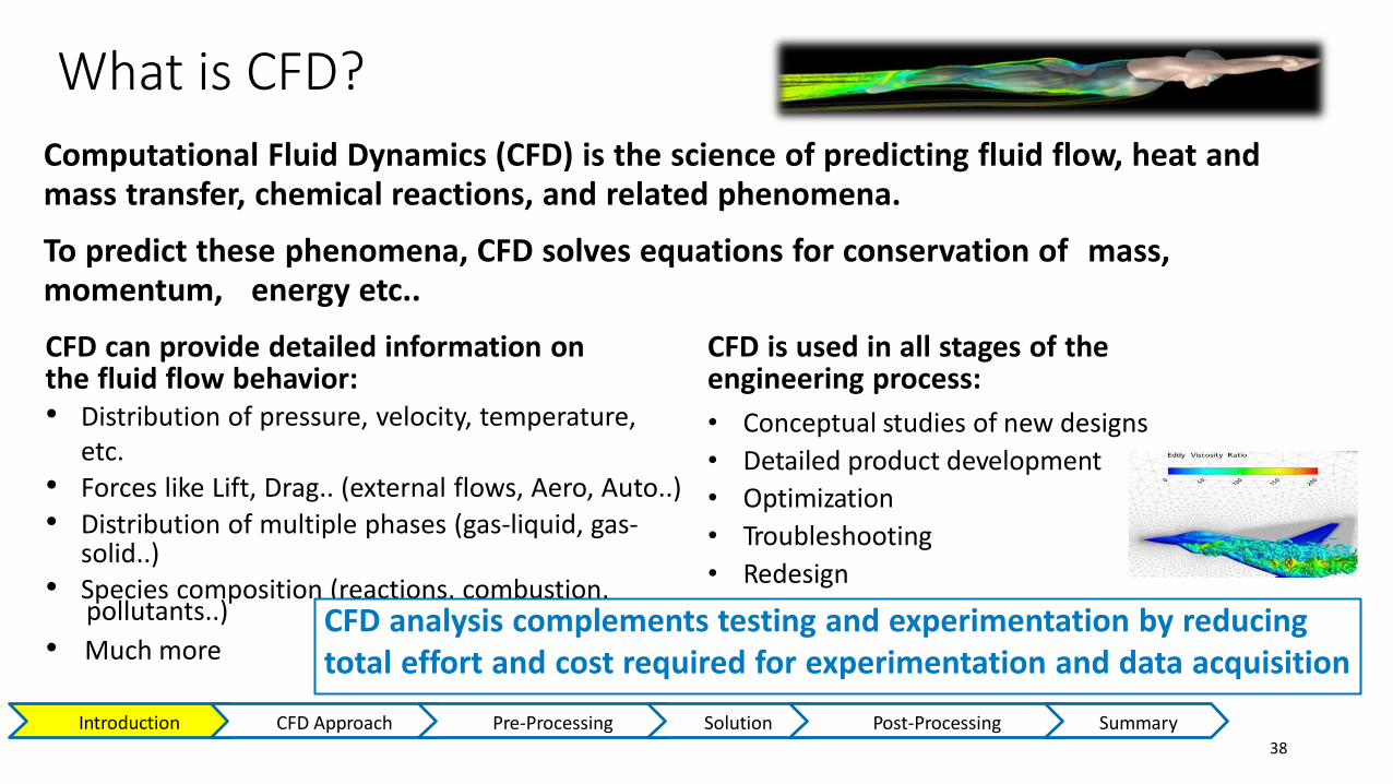
What is CFD?

38

Computational Fluid Dynamics (CFD) is the science of predicting fluid flow, heat andmass transfer, chemical reactions, and related phenomena.

To predict these phenomena, CFD solves equations for conservation of mass,momentum, energy etc..

CFD can provide detailed information onthe fluid flow behavior:• Distribution of pressure, velocity, temperature,

etc.

• Forces like Lift, Drag.. (external flows, Aero, Auto..)

• Distribution of multiple phases (gas-liquid, gas-solid..)

• Species composition (reactions, combustion,

• Much more

pollutants..)

CFD is used in all stages of theengineering process:

• Conceptual studies of new designs

• Detailed product development

• Optimization

• Troubleshooting

• Redesign

CFD analysis complements testing and experimentation by reducingtotal effort and cost required for experimentation and data acquisition


CFD Applications

39


CFD Applications

40


CFD Applications

41


CFD Applications

42


How Does CFD Work?

43

ANSYS CFD solvers are based on the finite volume method• Domain is discretized into a finite set of control volumes

• General conservation (transport) equations for mass, momentum, energy,species, etc. are solved on this set of control volumes

Unsteady Convection Diffusion Generation

• Partial differential equations are discretized into a system of algebraic equations

• All algebraic equations are then solved numerically to render the solution field

ControlVolume*

EquationContinuity

X momentumY momentumZ momentum

Energy

1

uvwh


Step 1. Define Your Modeling Goals

44

• What results are you looking for (i.e. pressure drop, mass flow rate),and how will they be used?

• What are your modeling options?• What simplifying assumptions can you make (i.e. symmetry, periodicity)?

• What simplifying assumptions do you have to make?

• What physical models will need to be included in your analysis

• What degree of accuracy is required?

• How quickly do you need the results?

• Is CFD an appropriate tool?


Step 2. Identify the Domain You Will Model

45

• How will you isolate a piece ofthe complete physical system?

• Where will the computational domainbegin and end?

− Do you have boundary condition information atthese boundaries?

− Can the boundary condition types accommodatethat information?

− Can you extend the domain to a point wherereasonable data exists?

• Can it be simplified or approximated asa 2D or axi-symmetric problem?

Domain of Interest asPart of a LargerSystem (not modeled)

Domain of interestisolated and meshedfor CFD simulation.

SummaryIntroduction CFD Approach Pre-Processing Solution Post-Processing

Step 3. Create a Solid Model of the Domain

46

• How will you obtain a model of the fluid region?− Make use of existing CAD models?

− Extract the fluid region from a solid part?

− Create from scratch?

• Can you simplify the geometry?− Remove unnecessary features that would complicate meshing;fillets, bolts…Ϳ?

− Make use of symmetry or periodicity?

• Are both the flow and boundary conditions symmetric /periodic?

• Do you need to split the model so that boundaryconditions or domains can be created?

Original CAD Part

ExtractedFluid Region


Step 4. Design and Create the Mesh

47

• What degree of mesh resolution is required in each region ofthe domain?

− Can you predict regions of high gradients?• The mesh must resolve geometric features of interest and capture gradients

of concern, e.g. velocity, pressure, temperature gradients

− Will you use adaption to add resolution?

• What type of mesh is most appropriate?− How complex is the geometry?

− Can you use a quad/hex mesh or is a tri/tet or hybrid mesh suitable?

− Are non-conformal interfaces needed?

• Do you have sufficient computer resources?− How many cells/nodes are required?

− How many physical models will be used?


48

Design and create the grid• Should you use a quad/hex grid, a tri/tet grid, a hybrid grid, or a non-

conformal grid?

• What degree of grid resolution is required in each region of the domain?

• How many cells are required for the problem?

• Will you use adaption to add resolution?

• Do you have sufficient computer memory?

triangle

quadrilateral

tetrahedron pyramid

prism or wedgehexahedronarbitrary polyhedron

Adaption example: final grid and solution

2D planar shell - final grid 2D planar shell - contours of pressure

final grid

33

Step 5. Set Up the Solver

50

• For a given problem, you will need to:

− Define material properties

• Fluid

• Solid

• Mixture

− Select appropriate physical models

• Turbulence, combustion, multiphase, etc.

− Prescribe operating conditions

− Prescribe boundary conditions at all boundary zones

− Provide initial values or a previous solution

− Set up solver controls

− Set up convergence monitors

Introduction CFD Approach Pre-Processing Solution

For complex problems solving a simplifiedor 2D problem will provide valuableexperience with the models and solversettings for your problem in a shortamount of time

Post-Processing Summary

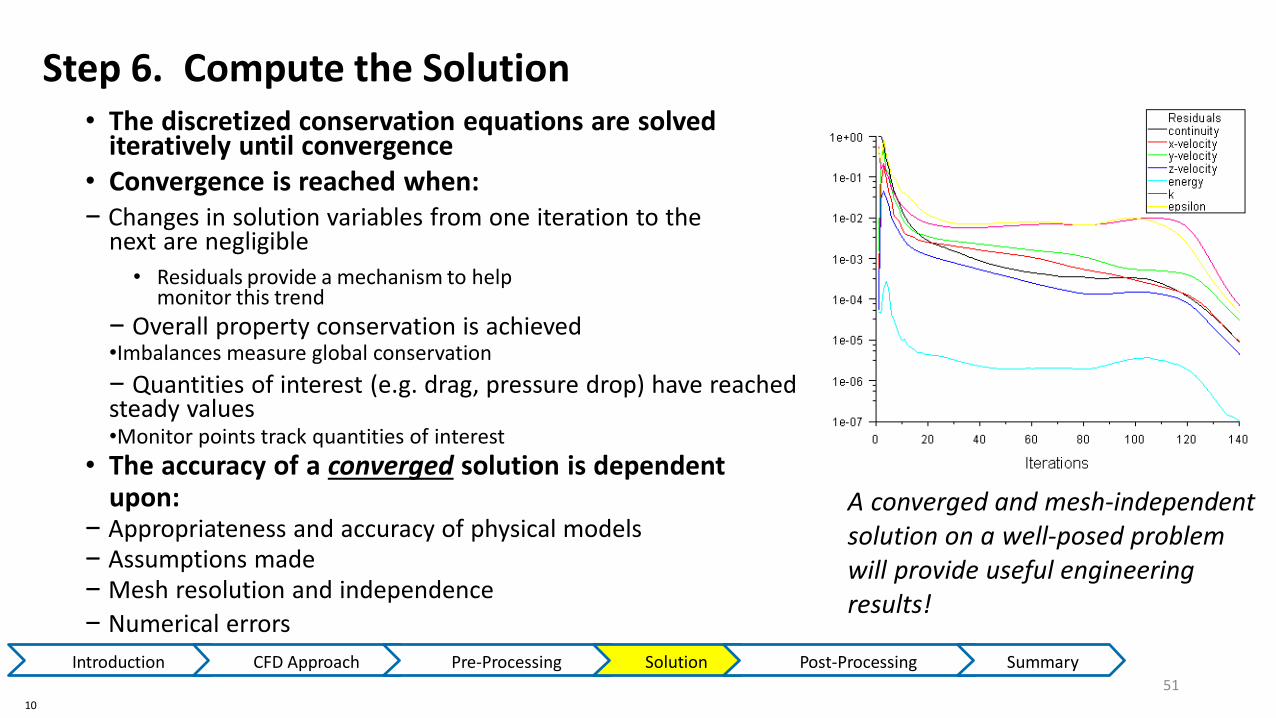
Step 6. Compute the Solution• The discretized conservation equations are solved

iteratively until convergence• Convergence is reached when:− Changes in solution variables from one iteration to the

next are negligible

• Residuals provide a mechanism to helpmonitor this trend

− Overall property conservation is achieved•Imbalances measure global conservation

− Quantities of interest (e.g. drag, pressure drop) have reachedsteady values•Monitor points track quantities of interest

• The accuracy of a converged solution is dependentupon:

− Appropriateness and accuracy of physical models− Assumptions made− Mesh resolution and independence

− Numerical errors

A converged and mesh-independentsolution on a well-posed problemwill provide useful engineeringresults!


10

51

Step 7. Examine the Results

52

• Examine the results to review solution andextract useful data

− Visualization Tools can be used to answer suchquestions as:

• What is the overall flow pattern?

• Is there separation?

• Where do shocks, shear layers, etc. form?

• Are key flow features being resolved?

− Numerical Reporting Tools can be used to calculatequantitative results:

• Forces and Moments

• Average heat transfer coefficients

• Surface and Volume integrated quantities

• Flux Balances

Examine results to ensure correct physical behavior andconservation of mass energy and other conservedquantities. High residuals may be caused by just a fewpoor quality cells.

Post-Processing SummaryIntroduction CFD Approach Pre-Processing Solution

Step 8. Consider Revisions to the Model

53

• Are the physical models appropriate?− Is the flow turbulent?− Is the flow unsteady?− Are there compressibility effects?

− Are there 3D effects?

• Are the boundary conditions correct?− Is the computational domain large enough?− Are boundary conditions appropriate?

− Are boundary values reasonable?

• Is the mesh adequate?− Does the solution change significantly with a refined mesh, or

is the solution mesh independent?− Does the mesh resolution of the geometry need to beimproved?− Does the model contain poor quality cells?

High residuals may be caused by justa few poor quality cells


Use CFD with Other Tools to Maximize its Effect

Prototype Testing Manufacturing

9.U

pd

ate

Mo

del

1. Define goals2. Identify domain

Pre-Processing

Problem Identification

3.4.5.6.

GeometryMesh PhysicsSolver Settings

7. Compute solution

Solve

8. Examine results

Post Processing

MeshCAD Geometry

Thermal Profile on Windshield

Final Optimized Design

Automated Optimization ofWindshield Defroster withANSYS DesignXplorer

54

Summary and Conclusions

55

• Summary:− All CFD simulations (in all mainstream CFD software products) areapproached using the steps just described

− Remember to first think about what the aims of the simulation areprior to creating the geometry and mesh

− Make sure the appropriate physical models are applied in the solver,and that the simulation is fully converged (more in a later lecture)

− Scrutinize the results, you may need to rework some of the earliersteps in light of the flow field obtained

1. Define Your ModelingGoals

2. Identify the Domain YouWill Model

3. Create a GeometricModel of the Domain

4. Design and Create theMesh

5. Set Up the Solver Settings6. Compute the Solution7. Examine the Results8. Consider Revisions to the

Model


56

Applications of CFD

• Applications of CFD are numerous!• Flow and heat transfer in industrial processes (boilers, heat exchangers,

combustion equipment, pumps, blowers, piping, etc.).

• Aerodynamics of ground vehicles, aircraft, missiles.

• Film coating, thermoforming in material processing applications.

• Flow and heat transfer in propulsion and power generation systems.

• Ventilation, heating, and cooling flows in buildings.

• Chemical vapor deposition (CVD) for integrated circuit manufacturing.

• Heat transfer for electronics packaging applications.

• And many, many more!

57

Advantages of CFD

• Relatively low cost.• Using physical experiments and tests to get essential engineering data for design can

be expensive.• CFD simulations are relatively inexpensive, and costs are likely to decrease as

computers become more powerful.

• Speed.• CFD simulations can be executed in a short period of time.• Quick turnaround means engineering data can be introduced early in the design

process.

• Ability to simulate real conditions.• Many flow and heat transfer processes can not be (easily) tested, e.g. hypersonic

flow.• CFD provides the ability to theoretically simulate any physical condition.

58

Advantages of CFD (2)

• Ability to simulate ideal conditions.• CFD allows great control over the physical process, and provides the ability to

isolate specific phenomena for study.

• Example: a heat transfer process can be idealized with adiabatic, constant heat flux, or constant temperature boundaries.

• Comprehensive information.• Experiments only permit data to be extracted at a limited number of locations

in the system (e.g. pressure and temperature probes, heat flux gauges, LDV, etc.).

• CFD allows the analyst to examine a large number of locations in the region of interest, and yields a comprehensive set of flow parameters for examination.

59

Limitations of CFD

• Physical models. • CFD solutions rely upon physical models of real world processes (e.g.

turbulence, compressibility, chemistry, multiphase flow, etc.).• The CFD solutions can only be as accurate as the physical models on which

they are based.

• Numerical errors.• Solving equations on a computer invariably introduces numerical errors.• Round-off error: due to finite word size available on the computer. Round-off

errors will always exist (though they can be small in most cases).• Truncation error: due to approximations in the numerical models. Truncation

errors will go to zero as the grid is refined. Mesh refinement is one way to deal with truncation error.

60

poor better

Fully Developed Inlet

Profile

Computational

Domain

Computational

Domain

Uniform Inlet

Profile

Limitations of CFD (2)

• Boundary conditions.• As with physical models, the accuracy of the CFD solution is only as good as

the initial/boundary conditions provided to the numerical model.

• Example: flow in a duct with sudden expansion. If flow is supplied to domain by a pipe, you should use a fully-developed profile for velocity rather than assume uniform conditions.

61

Summary

• CFD is a method to numerically calculate heat transfer and fluid flow.

• Currently, its main application is as an engineering method, to provide data that is complementary to theoretical and experimental data. This is mainly the domain of commercially available codes and in-house codes at large companies.

• CFD can also be used for purely scientific studies, e.g. into the fundamentals of turbulence. This is more common in academic institutions and government research laboratories. Codes are usually developed to specifically study a certain problem.

computational fluid mechanics lecture 1 · •finite difference method will be used to solve...

Documents